SynCoPation: Interactive Synthesis-Coupled Sound Propagation

Atul Rungta , Carl Schissler , Ravish Mehra , Chris Malloy , Ming Lin Fellow, IEEE , and Dinesh Manocha Fellow, IEEE

Department of Computer Science, University of North Carolina at Chapel HillURL: http://gamma.cs.unc.edu/syncopation

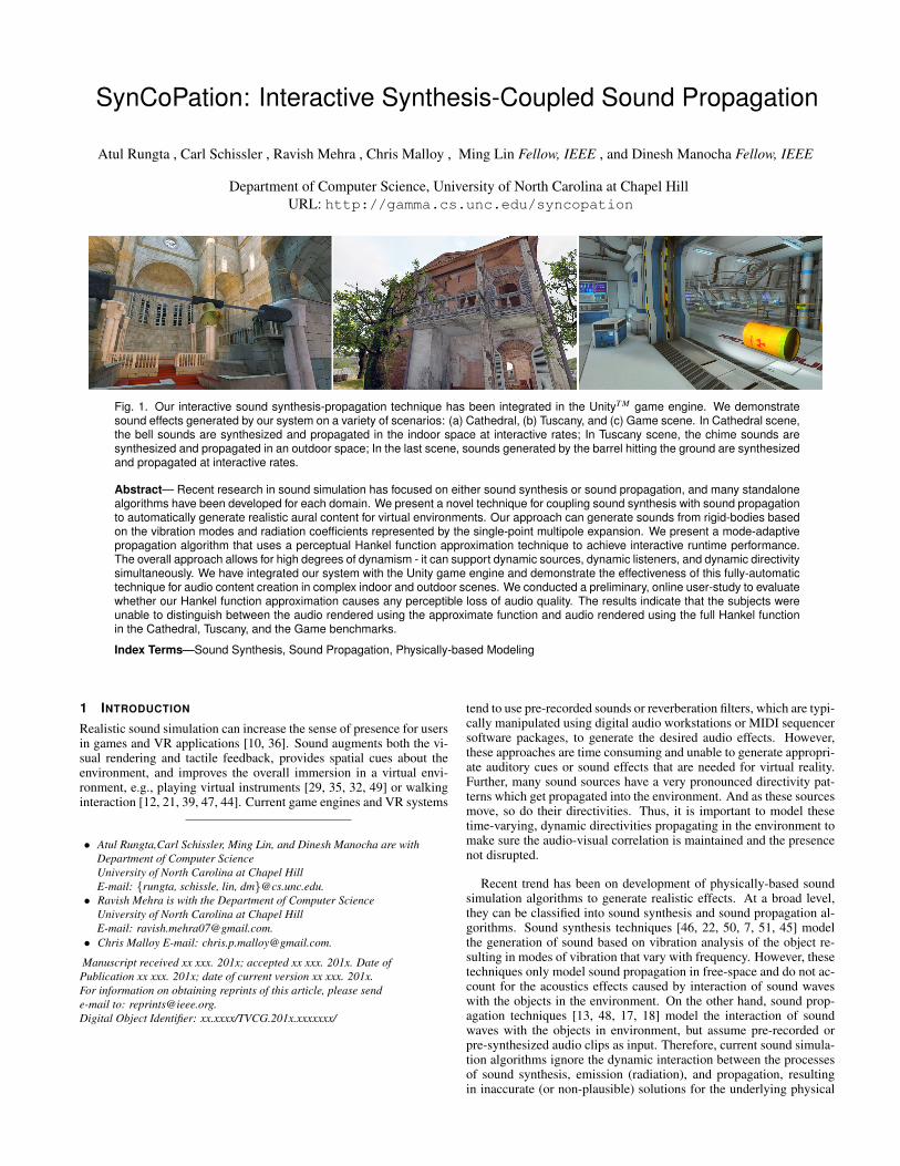
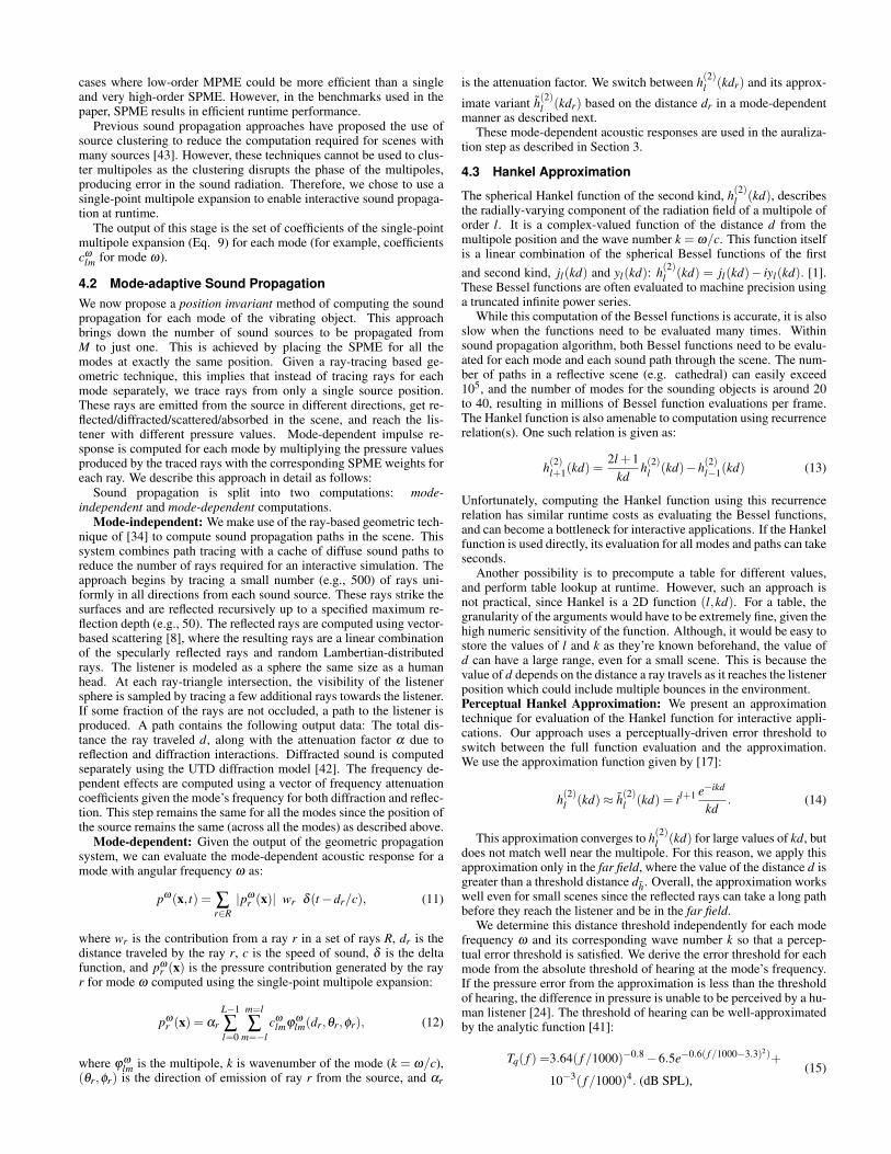
Fig. 1. Our interactive sound synthesis-propagation technique has been integrated in the UnityT M game engine. We demonstratesound effects generated by our system on a variety of scenarios: (a) Cathedral, (b) Tuscany, and (c) Game scene. In Cathedral scene,the bell sounds are synthesized and propagated in the indoor space at interactive rates; In Tuscany scene, the chime sounds aresynthesized and propagated in an outdoor space; In the last scene, sounds generated by the barrel hitting the ground are synthesizedand propagated at interactive rates.

Abstract— Recent research in sound simulation has focused on either sound synthesis or sound propagation, and many standalonealgorithms have been developed for each domain. We present a novel technique for coupling sound synthesis with sound propagationto automatically generate realistic aural content for virtual environments. Our approach can generate sounds from rigid-bodies basedon the vibration modes and radiation coefficients represented by the single-point multipole expansion. We present a mode-adaptivepropagation algorithm that uses a perceptual Hankel function approximation technique to achieve interactive runtime performance.The overall approach allows for high degrees of dynamism - it can support dynamic sources, dynamic listeners, and dynamic directivitysimultaneously. We have integrated our system with the Unity game engine and demonstrate the effectiveness of this fully-automatictechnique for audio content creation in complex indoor and outdoor scenes. We conducted a preliminary, online user-study to evaluatewhether our Hankel function approximation causes any perceptible loss of audio quality. The results indicate that the subjects wereunable to distinguish between the audio rendered using the approximate function and audio rendered using the full Hankel functionin the Cathedral, Tuscany, and the Game benchmarks.

Index Terms—Sound Synthesis, Sound Propagation, Physically-based Modeling

1 INTRODUCTION

Realistic sound simulation can increase the sense of presence for usersin games and VR applications [10, 36]. Sound augments both the vi-sual rendering and tactile feedback, provides spatial cues about theenvironment, and improves the overall immersion in a virtual envi-ronment, e.g., playing virtual instruments [29, 35, 32, 49] or walkinginteraction [12, 21, 39, 47, 44]. Current game engines and VR systems

• Atul Rungta,Carl Schissler, Ming Lin, and Dinesh Manocha are withDepartment of Computer ScienceUniversity of North Carolina at Chapel HillE-mail: rungta, schissle, lin, dm@cs.unc.edu.

• Ravish Mehra is with the Department of Computer ScienceUniversity of North Carolina at Chapel HillE-mail: ravish.mehra07@gmail.com.

• Chris Malloy E-mail: chris.p.malloy@gmail.com.

Manuscript received xx xxx. 201x; accepted xx xxx. 201x. Date ofPublication xx xxx. 201x; date of current version xx xxx. 201x.For information on obtaining reprints of this article, please sende-mail to: reprints@ieee.org.Digital Object Identifier: xx.xxxx/TVCG.201x.xxxxxxx/

tend to use pre-recorded sounds or reverberation filters, which are typi-cally manipulated using digital audio workstations or MIDI sequencersoftware packages, to generate the desired audio effects. However,these approaches are time consuming and unable to generate appropri-ate auditory cues or sound effects that are needed for virtual reality.Further, many sound sources have a very pronounced directivity pat-terns which get propagated into the environment. And as these sourcesmove, so do their directivities. Thus, it is important to model thesetime-varying, dynamic directivities propagating in the environment tomake sure the audio-visual correlation is maintained and the presencenot disrupted.

Recent trend has been on development of physically-based soundsimulation algorithms to generate realistic effects. At a broad level,they can be classified into sound synthesis and sound propagation al-gorithms. Sound synthesis techniques [46, 22, 50, 7, 51, 45] modelthe generation of sound based on vibration analysis of the object re-sulting in modes of vibration that vary with frequency. However, thesetechniques only model sound propagation in free-space and do not ac-count for the acoustics effects caused by interaction of sound waveswith the objects in the environment. On the other hand, sound prop-agation techniques [13, 48, 17, 18] model the interaction of soundwaves with the objects in environment, but assume pre-recorded orpre-synthesized audio clips as input. Therefore, current sound simula-tion algorithms ignore the dynamic interaction between the processesof sound synthesis, emission (radiation), and propagation, resultingin inaccurate (or non-plausible) solutions for the underlying physical

processes. For example, consider the case of a kitchen bowl fallingfrom a countertop; the change in the directivity of the bowl with differ-ent hit positions and the effect of this time-varying, mode-dependentdirectivity on the propagated sound in the environment is mostly ig-nored by the current sound simulation techniques. Similarly, for abarrel rolling down the alley, the sound consists of multiple modes,where each mode has a time-varying radiation and propagation char-acteristic that depends on the hit positions on the barrel along withthe instantaneous position and orientation of the barrel. Moreover, theinteraction of the resulting sound waves with the walls of the alleycause resonances at certain frequencies and damping at others. Cur-rent sound simulation techniques model the barrel as a sound sourcewith either static, mode-independent directivity, and model the result-ing propagation in the environment with a mode-independent acousticresponse or model the time-varying directivity of the barrel but prop-agate those in free-space only [7]. Due to these limitations, artists andgame audio-designers have to manually design sound effects corre-sponding to these different scenarios, which can be very tedious andtime-consuming [28].Main Results: In this paper, we present the first coupled synthesis-propagation algorithm which models the entire process of sound sim-ulation starting from the surface vibration of rigid objects, radiationof sound waves from these surface vibrations, and interaction of theresulting sound waves with the virtual environment for interactive ap-plications. The key insights of our work is the use of a single-pointmultipole expansion (SPME) to couple the radiation and propagationcharacteristics of a source for each vibration mode. Mathematically, asingle-point multipole corresponds to a single radiating source placedinside the object; this expansion significantly reduces the computa-tional cost of the propagation stage compared to a multi-point mul-tipole expansion. Moreover, we present a novel interactive mode-adaptive sound propagation technique that uses ray tracing to com-pute the per-mode impulse responses for a source-listener position.We also describe a novel perceptually-driven Hankel function approx-imation scheme that reduces the computational cost of this mode-adaptive propagation to enable interactive performance for virtual en-vironments. The main benefits of our approach include:

1. Per-mode coupling of synthesis and propagation through the useof single-point multipole expansion.

2. Interactive mode-adaptive propagation technique based onperceptually-driven Hankel function approximation.

3. High degree of dynamism to model dynamic surface vibrations,sound radiation and propagation for moving sources and listen-ers.

Our technique performs end-to-end sound simulation from firstprinciples and enables automatic sound effect generation for inter-active applications, thereby reducing the manual effort and the time-spent by artists and game-audio designers. Our system can automati-cally model the complex acoustic effects generated in various dynamicscenarios such as (a) swinging church bell inside a reverberant cathe-dral, (b) swaying wind chimes on the balcony of Tuscany countrysidehouse, (c) a metal barrel falling downstairs in an indoor game sceneand (d) orchestra playing music in a concert hall, at 10fps or fasteron a multi-core desktop PC. We have integrated our technique withthe UnityT M game engine and demonstrated complex sound effectsenabled by our coupled synthesis-propagation technique in differentscenarios (see Fig. 1).

Furthermore, we evaluated the effectiveness of our perceptual Han-kel approximation algorithm by performing a preliminary user-study.The study was an online one where the subjects where shown snip-pets of three benchmarks ( Cathedral, Tuscany, and Game ) with au-dio delivered through headphones/earphones and rendered using ourperceptual Hankel approximation and using no approximation. Thesubjects were asked to judge the similarity between the two sounds forthe three benchmarks. Initial results show that the subjects were un-able to distinguish between the two sounds indicating that our Hankel

approximation doesn’t compromise on the audio quality in a percepti-ble way.

2 RELATED WORK AND BACKGROUND

In this section, we give an overview of sound synthesis, radiation, andpropagation and survey some relevant work.

2.1 Sound Synthesis for rigid-bodiesGiven a rigid body, sound synthesis techniques solve the modal dis-placement equation

Kd+Cd+Md = f, (1)

where K, C, and M are the stiffness, damping, and mass matrices,respectively and f represents the (external) force vector. This givesa discrete set of mode shapes di, their modal frequencies ωi, and theamplitudes qi(t). The vibration’s displacement vector is given by:

d(t) = Uq(t)≡ [d1, ..., ˆdM ]q(t), (2)

where M is total number of modes and q(t) ∈ ℜM is the vector ofmodal amplitude coefficients qi(t) expressed as a bank of sinusoids:

qi(t) = aie−ditsin(2π fit +θi), (3)

where fi is the modal frequency (in Hz.), di is the damping coefficient,ai is amplitude, and θi is the initial phase.

[2] introduced modal analysis approach to synthesizing sounds.[46] introduced a measurement-driven method to determine the modesof vibration and their dependence on the point of impact for a givenshape. Later, [22] were able to model arbitrarily shaped objects andsimulate realistic sounds for a few of these objects at interactive rates.This approach is called the modal analysis and requires an expensiveprecomputation, but achieves interactive runtime performance. Thenumber of modes generated tend to increase with the geometric com-plexity of the objects. [27] used a system of spring-mass along withperceptually motivated acceleration techniques to generate realisticsound effects for hundreds of objects in real time. [31] developeda contact model to capture multi-level surface characteristics based on[27]. Recent work on modal synthesis also uses the single point mul-tipole expansion [51].

2.2 Sound Radiation and PropagationSound propagation in frequency domain is described using theHelmholtz equation

∇2 p+

ω2

c2 p = 0, x ∈Ω, (4)

where p = p(x,ω) is the complex-valued pressure field, ω is the an-gular frequency, c is the speed of sound in the medium, and ∇2 isthe Laplacian operator. To simplify the notation, we hide the depen-dence on angular frequency and represent the pressure field as p(x).Boundary conditions are specified on the boundary of the domain ∂Ω

by either the Dirichlet boundary condition that specifies the pressureon the boundary p = f (x) on ∂Ω, the Nuemann boundary conditionthat specifies the velocity of the medium ∂ p(x)

∂n = f (x) on ∂Ω, or

a mixed boundary condition that specifies Z ∈ C, so that Z ∂ p(x)∂n =

f (x) on ∂Ω. The boundary condition at infinity is also specified us-ing the Sommerfeld radiation condition [25]

limr→∞

[∂ p∂ r

+ iω

cp] = 0, (5)

where r = ||x|| is the distance of point x from the origin.Equivalent Sources: The uniqueness of the acoustic boundary

value problem guarantees that the solution of the free-space Helmholtzequation along with the specified boundary conditions is unique insideΩ [23]. The unique solution p(x) can be found by expressing the so-lution as a linear combination of fundamental solutions. One choice

of fundamental solutions is based on equivalent sources. An equiva-lent source q(x,yi) is the solution of the Helmholtz equation subjectto the Sommerfeld radiation condition. Here x is the point of evalua-tion, yi is the source position and xi 6= yi. The equivalent source canbe expressed as:

q(x,yi) =L−1

∑l=0

l

∑m=−l

cilmϕlm(x,yi) =L2

∑k=1

eikϕk(x,yi), (6)

where k is a generalized index for (l,m), ϕk are multipole functions,and cilm is the strength of multipoles. Multipoles are given as a productof two functions:

ϕlm(x,yi) = Γlmh(2)l (kdi)ψlm(θi,φi), (7)

where (di,θi,φi) is the vector (x− yi) expressed in spherical coordi-nates, h2

l is the spherical Hankel function of the second kind, k is thewavenumber given by ω

c , ψlm(θi,φi) are the complex-valued sphericalharmonics functions, and Γlm is the normalizing factor for the spheri-cal harmonics.

2.2.1 Sound RadiationThe Helmholtz equation is the mathematical way to model sound ra-diation from vibrating rigid bodies. Boundary element method is awidely used method for solving acoustic radiation problems [9] buthas a major drawback in terms of high memory requirements. An ef-ficient technique known as the Equivalent source method (ESM) [23]exploits the uniqueness of the solutions to the acoustic boundary valueproblem. ESM expresses the solution field as a linear combinationof equivalent sources of various orders (monopoles, dipoles, etc.) byplacing these simple sources at variable locations inside the object andmatching the boundary conditions on the object’s surface, guarantee-ing the correctness of solution. The pressure at any point in Ω due toN equivalent sources located at yiN

i=1 can be expressed as a linearcombination:

p(x) =N

∑i=1

L−1

∑l=0

m=l

∑m=−l

cilmϕlm(x,yi). (8)

This compact representation of the pressure p(x) makes it possible toevaluate the pressure at any point of the domain in an efficient manner.This is also known as the multi-point multipole expansion. Typically,this expansion uses a large number of low-order multipoles (L = 1or 2) placed at different locations inside the object to represent thepressure field. [14] use this multi-point expansion to represent theradiated pressure field generated by a vibrating object. Another variantof this, is the single-point multipole expansion represented as

p(x) =L−1

∑l=0

m=l

∑m=−l

clmϕlm(x,y). (9)

discussed in [23]. In this expansion, only a single multipole of highorder is placed inside the object to match outgoing radiation field.

2.2.2 Geometric Sound PropagationGeometric sound propagation techniques use the simplifying assump-tion that the wavelength of sound is much smaller than the featureson the objects in the scene. As a result, these methods are most ac-curate for high frequencies and approximately model low-frequencyeffects like diffraction and scattering as separate phenomena. Com-monly used techniques are based on image source methods and raytracing. Recently, there has been a focus on computing realistic acous-tics in real-time using algorithms designed for fast simulation. Theseinclude beam tracing [13] and ray-based algorithms [16, 40] to com-pute specular an diffuse reflections and can be extended to approx-imate edge diffraction. Diffuse reflections can also be modeled us-ing acoustic rendering equation [37, 4]. In addition, frame-to-framecoherence of the sound field can be utilized to achieve a significantspeedup [34].

2.3 Coupled Synthesis-Propagation

Ren et al. [29] presented an interactive virtual percussion instrumentsystem that used modal synthesis as well as numerical sound propaga-tion for modeling a small instrument cavity. However, the couplingproposed in this system did not incorporate a time-varying, mode-dependent radiation and propagation characteristic of the musical in-struments. Additionally, this system only modeled propagation insidethe acoustic space of the instrument and not the full 3D environment.Furthermore, the volume of the underlying acoustic spaces (instru-ments) in [29] was rather small in comparison to the typical scenesshown in this paper (see Fig. 1).

3 OVERVIEW

In this section, we provide an overview of our mode-adaptive, coupledsynthesis-propagation technique (see Figure 2).

The overall technique can be split into two main stages: preprocess-ing and runtime. In the preprocessing stage, we start with the vibrationanalysis of each rigid object to compute its modes of vibrations. Thisstep is performed using the finite element analysis of the object meshto compute displacements (or shapes), frequencies, and amplitudes ofall the modes of vibration. The next step is to compute the sound radia-tion field corresponding to each mode. This is done by using the modeshapes as the boundary condition for the free-space Helmholtz equa-tion and solving it using the state-of-the-art boundary element method(BEM). This step computes the outgoing radiation field correspond-ing to each vibration mode. To enable interactive evaluation at run-time, the outgoing radiation fields are represented compactly usingthe single-point multipole expansion [23]. This representation signif-icantly reduces the runtime computational cost for sound propagationby limiting the number of multipole sources to one per mode insteadof hundreds or even thousands per mode in the case of multi-pointmultipole expansion [23, 14]. This completes our preprocessing step.The coefficients of the single-point multipole expansion are stored forruntime use.

At runtime, we use a mode-adaptive sound propagation techniquethat uses the single-point multipole expansion as the sound sourcefor computing sound propagation corresponding to each vibrationmode. In order to achieve interactive performance, we use a novelperceptually-driven Hankel function approximation. The sound prop-agation technique computes the impulse response corresponding tothe instantaneous position for source-listener pair for each vibrationmode. High modal frequencies are propagated using the geometricsound propagation techniques. Low modal frequencies can be prop-agated using the wave-based techniques. Hybrid techniques combinegeometric and wave-based techniques to perform sound propagationin the entire frequency range. The final stage of the pipeline takes theimpulse response for each mode, convolves it with that mode’s am-plitude, and sums it for all the modes to give the final audio at thelistener.

We now describe each stage of the pipeline in detail.Modal Analysis: We adopt a finite element method [22] to precom-

pute the modes of vibration of an object. In this step, we first discretizethe object into a tetrahedral mesh and solve the modal displacementequation (Eq. 1) analytically under the Raleigh-damping assumption(i.e. damping matrix C can be written as a linear combination of stiff-ness K and mass matrix M). This facilitates the diagonalization ofthe modal displacement equation, which can then be represented as ageneralized eigenvalue problem and solved analytically as system ofdecoupled oscillators. The output of this step is the vibration modes ofthe object along with the modal displacements, frequencies, and am-plitudes. [30] showed that the Raleigh damping model is a suitablegeometry-invariant sound model and is therefore a suitable choice forour damping model.

Sound Radiation: This step computes the sound radiation charac-teristic of the vibration modes of each object by solving the free-spaceHelmholtz equation [14]. The modal displacements of each modeserves as the boundary condition for the Helmholtz equation. Theboundary element method (BEM) is then used to solve the Helmholtz

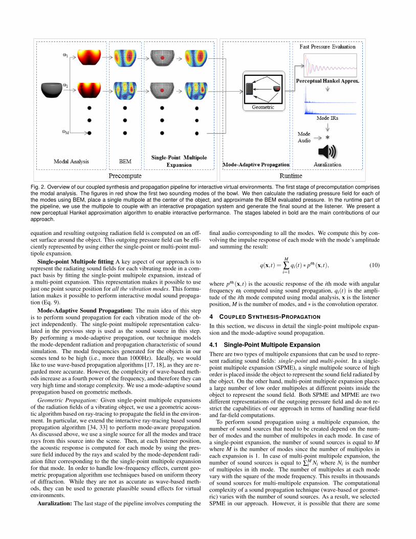
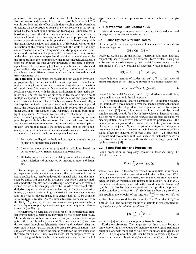
Fig. 2. Overview of our coupled synthesis and propagation pipeline for interactive virtual environments. The first stage of precomputation comprisesthe modal analysis. The figures in red show the first two sounding modes of the bowl. We then calculate the radiating pressure field for each ofthe modes using BEM, place a single multipole at the center of the object, and approximate the BEM evaluated pressure. In the runtime part ofthe pipeline, we use the multipole to couple with an interactive propagation system and generate the final sound at the listener. We present anew perceptual Hankel approximation algorithm to enable interactive performance. The stages labeled in bold are the main contributions of ourapproach.

equation and resulting outgoing radiation field is computed on an off-set surface around the object. This outgoing pressure field can be effi-ciently represented by using either the single-point or multi-point mul-tipole expansion.

Single-point Multipole fitting A key aspect of our approach is torepresent the radiating sound fields for each vibrating mode in a com-pact basis by fitting the single-point multipole expansion, instead ofa multi-point expansion. This representation makes it possible to usejust one point source position for all the vibration modes. This formu-lation makes it possible to perform interactive modal sound propaga-tion (Eq. 9).

Mode-Adaptive Sound Propagation: The main idea of this stepis to perform sound propagation for each vibration mode of the ob-ject independently. The single-point multipole representation calcu-lated in the previous step is used as the sound source in this step.By performing a mode-adaptive propagation, our technique modelsthe mode-dependent radiation and propagation characteristic of soundsimulation. The modal frequencies generated for the objects in ourscenes tend to be high (i.e., more than 1000Hz). Ideally, we wouldlike to use wave-based propagation algorithms [17, 18], as they are re-garded more accurate. However, the complexity of wave-based meth-ods increase as a fourth power of the frequency, and therefore they canvery high time and storage complexity. We use a mode-adaptive soundpropagation based on geometric methods.

Geometric Propagation: Given single-point multipole expansionsof the radiation fields of a vibrating object, we use a geometric acous-tic algorithm based on ray-tracing to propagate the field in the environ-ment. In particular, we extend the interactive ray-tracing based soundpropagation algorithm [34, 33] to perform mode-aware propagation.As discussed above, we use a single source for all the modes and tracerays from this source into the scene. Then, at each listener position,the acoustic response is computed for each mode by using the pres-sure field induced by the rays and scaled by the mode-dependent radi-ation filter corresponding to the the single-point multipole expansionfor that mode. In order to handle low-frequency effects, current geo-metric propagation algorithm use techniques based on uniform theoryof diffraction. While they are not as accurate as wave-based meth-ods, they can be used to generate plausible sound effects for virtualenvironments.

Auralization: The last stage of the pipeline involves computing the

final audio corresponding to all the modes. We compute this by con-volving the impulse response of each mode with the mode’s amplitudeand summing the result:

q(x, t) =M

∑i=1

qi(t)∗ pωi(x, t), (10)

where pωi(x, t) is the acoustic response of the ith mode with angularfrequency ωi computed using sound propagation, qi(t) is the ampli-tude of the ith mode computed using modal analysis, x is the listenerposition, M is the number of modes, and ∗ is the convolution operator.

4 COUPLED SYNTHESIS-PROPAGATION

In this section, we discuss in detail the single-point multipole expan-sion and the mode-adaptive sound propagation.

4.1 Single-Point Multipole ExpansionThere are two types of multipole expansions that can be used to repre-sent radiating sound fields: single-point and multi-point. In a single-point multipole expansion (SPME), a single multipole source of highorder is placed inside the object to represent the sound field radiated bythe object. On the other hand, multi-point multipole expansion placesa large number of low order multipoles at different points inside theobject to represent the sound field. Both SPME and MPME are twodifferent representations of the outgoing pressure field and do not re-strict the capabilities of our approach in terms of handling near-fieldand far-field computations.

To perform sound propagation using a multipole expansion, thenumber of sound sources that need to be created depend on the num-ber of modes and the number of multipoles in each mode. In case ofa single-point expansion, the number of sound sources is equal to Mwhere M is the number of modes since the number of multipoles ineach expansion is 1. In case of multi-point multipole expansion, thenumber of sound sources is equal to ∑

Mi Ni where Ni is the number

of multipoles in ith mode. The number of multipoles at each modevary with the square of the mode frequency. This results in thousandsof sound sources for multi-multipole expansion. The computationalcomplexity of a sound propagation technique (wave-based or geomet-ric) varies with the number of sound sources. As a result, we selectedSPME in our approach. However, it is possible that there are some

cases where low-order MPME could be more efficient than a singleand very high-order SPME. However, in the benchmarks used in thepaper, SPME results in efficient runtime performance.

Previous sound propagation approaches have proposed the use ofsource clustering to reduce the computation required for scenes withmany sources [43]. However, these techniques cannot be used to clus-ter multipoles as the clustering disrupts the phase of the multipoles,producing error in the sound radiation. Therefore, we chose to use asingle-point multipole expansion to enable interactive sound propaga-tion at runtime.

The output of this stage is the set of coefficients of the single-pointmultipole expansion (Eq. 9) for each mode (for example, coefficientscω

lm for mode ω).

4.2 Mode-adaptive Sound PropagationWe now propose a position invariant method of computing the soundpropagation for each mode of the vibrating object. This approachbrings down the number of sound sources to be propagated fromM to just one. This is achieved by placing the SPME for all themodes at exactly the same position. Given a ray-tracing based ge-ometric technique, this implies that instead of tracing rays for eachmode separately, we trace rays from only a single source position.These rays are emitted from the source in different directions, get re-flected/diffracted/scattered/absorbed in the scene, and reach the lis-tener with different pressure values. Mode-dependent impulse re-sponse is computed for each mode by multiplying the pressure valuesproduced by the traced rays with the corresponding SPME weights foreach ray. We describe this approach in detail as follows:

Sound propagation is split into two computations: mode-independent and mode-dependent computations.

Mode-independent: We make use of the ray-based geometric tech-nique of [34] to compute sound propagation paths in the scene. Thissystem combines path tracing with a cache of diffuse sound paths toreduce the number of rays required for an interactive simulation. Theapproach begins by tracing a small number (e.g., 500) of rays uni-formly in all directions from each sound source. These rays strike thesurfaces and are reflected recursively up to a specified maximum re-flection depth (e.g., 50). The reflected rays are computed using vector-based scattering [8], where the resulting rays are a linear combinationof the specularly reflected rays and random Lambertian-distributedrays. The listener is modeled as a sphere the same size as a humanhead. At each ray-triangle intersection, the visibility of the listenersphere is sampled by tracing a few additional rays towards the listener.If some fraction of the rays are not occluded, a path to the listener isproduced. A path contains the following output data: The total dis-tance the ray traveled d, along with the attenuation factor α due toreflection and diffraction interactions. Diffracted sound is computedseparately using the UTD diffraction model [42]. The frequency de-pendent effects are computed using a vector of frequency attenuationcoefficients given the mode’s frequency for both diffraction and reflec-tion. This step remains the same for all the modes since the position ofthe source remains the same (across all the modes) as described above.

Mode-dependent: Given the output of the geometric propagationsystem, we can evaluate the mode-dependent acoustic response for amode with angular frequency ω as:

pω (x, t) = ∑r∈R|pω

r (x)| wr δ (t−dr/c), (11)

where wr is the contribution from a ray r in a set of rays R, dr is thedistance traveled by the ray r, c is the speed of sound, δ is the deltafunction, and pω

r (x) is the pressure contribution generated by the rayr for mode ω computed using the single-point multipole expansion:

pωr (x) = αr

L−1

∑l=0

m=l

∑m=−l

cωlmϕ

ωlm(dr,θr,φr), (12)

where ϕωlm is the multipole, k is wavenumber of the mode (k = ω/c),

(θr,φr) is the direction of emission of ray r from the source, and αr

is the attenuation factor. We switch between h(2)l (kdr) and its approx-

imate variant h(2)l (kdr) based on the distance dr in a mode-dependentmanner as described next.

These mode-dependent acoustic responses are used in the auraliza-tion step as described in Section 3.

4.3 Hankel Approximation

The spherical Hankel function of the second kind, h(2)l (kd), describesthe radially-varying component of the radiation field of a multipole oforder l. It is a complex-valued function of the distance d from themultipole position and the wave number k = ω/c. This function itselfis a linear combination of the spherical Bessel functions of the firstand second kind, jl(kd) and yl(kd): h(2)l (kd) = jl(kd)− iyl(kd). [1].These Bessel functions are often evaluated to machine precision usinga truncated infinite power series.

While this computation of the Bessel functions is accurate, it is alsoslow when the functions need to be evaluated many times. Withinsound propagation algorithm, both Bessel functions need to be evalu-ated for each mode and each sound path through the scene. The num-ber of paths in a reflective scene (e.g. cathedral) can easily exceed105, and the number of modes for the sounding objects is around 20to 40, resulting in millions of Bessel function evaluations per frame.The Hankel function is also amenable to computation using recurrencerelation(s). One such relation is given as:

h(2)l+1(kd) =2l +1

kdh(2)l (kd)−h(2)l−1(kd) (13)

Unfortunately, computing the Hankel function using this recurrencerelation has similar runtime costs as evaluating the Bessel functions,and can become a bottleneck for interactive applications. If the Hankelfunction is used directly, its evaluation for all modes and paths can takeseconds.

Another possibility is to precompute a table for different values,and perform table lookup at runtime. However, such an approach isnot practical, since Hankel is a 2D function (l,kd). For a table, thegranularity of the arguments would have to be extremely fine, given thehigh numeric sensitivity of the function. Although, it would be easy tostore the values of l and k as they’re known beforehand, the value ofd can have a large range, even for a small scene. This is because thevalue of d depends on the distance a ray travels as it reaches the listenerposition which could include multiple bounces in the environment.Perceptual Hankel Approximation: We present an approximationtechnique for evaluation of the Hankel function for interactive appli-cations. Our approach uses a perceptually-driven error threshold toswitch between the full function evaluation and the approximation.We use the approximation function given by [17]:

h(2)l (kd)≈ h(2)l (kd) = il+1 e−ikd

kd. (14)

This approximation converges to h(2)l (kd) for large values of kd, butdoes not match well near the multipole. For this reason, we apply thisapproximation only in the far field, where the value of the distance d isgreater than a threshold distance dh. Overall, the approximation workswell even for small scenes since the reflected rays can take a long pathbefore they reach the listener and be in the far field.

We determine this distance threshold independently for each modefrequency ω and its corresponding wave number k so that a percep-tual error threshold is satisfied. We derive the error threshold for eachmode from the absolute threshold of hearing at the mode’s frequency.If the pressure error from the approximation is less than the thresholdof hearing, the difference in pressure is unable to be perceived by a hu-man listener [24]. The threshold of hearing can be well-approximatedby the analytic function [41]:

Tq( f ) =3.64( f/1000)−0.8−6.5e−0.6( f/1000−3.3)2)+

10−3( f/1000)4. (dB SPL),(15)

SPL stands for Sound Pressure Level and is measured in decibels (dB).In a preprocessing step, we evaluate this function at each mode’s

frequency to determine a per-mode error threshold, and then deter-mine the distance threshold dh where the approximation is perceptu-ally valid for the mode. This information is computed and stored foreach sounding object. At runtime, when the pressure contribution foreach path i is computed, we use the original Hankel h(2)l (kidi) when

di < dh and the approximation h(2)l (kidi) when di ≥ dh.We would like to note that although the approximation to Hankel

function specified in Eq 14 is standard, the novelty of our approachlies in the way we use it. As described above, we use perceptually-driven thresholds to decide when to automatically switch to the ap-proximate version. We also did a user-evaluation to make sure theperceptually-motivated approximation doesn’t cause any loss of qual-ity in our context. The details of the evaluation are presented in theSection 5.

-20

-10

0

10

20

30

40

50

60

0 50 100 150 200 250 300

Erro

r, H

anke

l app

roxi

mat

ion

(dB

SPL

)

r (m)

Error, Hankel Approx.

5 dB SPL error threshold

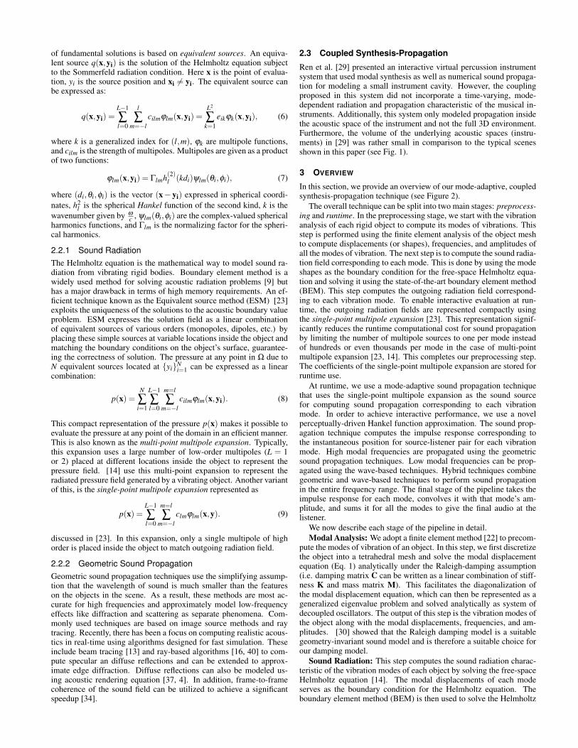
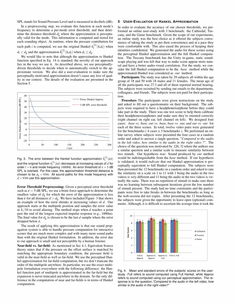
Fig. 3. The error between the Hankel function approximation h(2)l (kd)

and the original function h(2)l (kd) decreases at increasing values of d fororder l = 6 and mode frequency 1000Hz. An error threshold of ε = 5 dBSPL is overlaid. For this case, the approximation threshold distance ischosen to be dh = 93m. All sound paths for this mode frequency withd > 93m use this approximation.

Error Threshold Preprocessing: Given a perceptual error thresholdsuch as ε = 5 dB SPL, we use a brute-force approach to determine thesmallest value of dh for which the error of the approximation is lessthan ε for all distances d > dh. We have included Figure 3 that showsan example of how the error shrinks at increasing values of d. Ourapproach starts at the multipole position and samples the error valueat λ/10 to avoid aliasing. The method stops when d reaches a pointpast the end of the longest expected impulse response (e.g., 1000m).The final value for dh is chosen to be the last d sample where the errordropped below ε .

The result of applying this approximation is that our sound prop-agation system is able to handle pressure computation for interactivescenes that are much more complex and with many more sound pathsthan with the original Hankel formulation. In addition, the error dueto our approach is small and not perceptible by a human listener.Near-field vs. far-field: As mentioned in Sec 4.1, Equivalent Sourcetheory states that if the pressure on the offset surface is matched bymatching the appropriate boundary condition, the pressure field isvalid in the near-field as well as far-field. We use the perceptual Han-kel approximation for far-field computation, but we don’t truncate theorder of the multipole anywhere. In particular, we use the exact multi-pole formulation everywhere with the following difference: the Han-kel function part of multipole is approximated in the far-field but theexpansion is never truncated anywhere in the domain. So the only dif-ference in the computation of near and far-fields is in terms of Hankelcomputation.

5 USER-EVALUATION OF HANKEL APPROXIMATION

In order to evaluate the accuracy of our chosen thresholds, we per-formed an online user-study with 3 benchmark: the Cathredal, Tus-cany, and the Game benchmark. Given the scope of our experiments,an online study was the best choice as it offered the subjects conve-nience of taking the study as per their convenience and at a pace theywere comfortable with. This also eased the process of keeping theiridentities confidential. We generated the audio for these scenes usingthe perceptual Hankel approximation and the full Hankel computa-tion. The Tuscany benchmark has the Unity in-game, static sound-scape playing and was left that way to make scene appear more natu-ral and have a better audio-visual correlation. For the study, we con-sider the full Hankel computation to be the base method while theapproximated-Hankel was considered as our method.

Participants The study was taken by 29 subjects all within the agegroup of 18 and 50 with 18 males and 11 females. The mean age ofall the participants was 27.3 and all of them reported normal hearing.The subjects were recruited by sending out emails to the departments,colleagues, and friends. The subjects were not paid for their participa-tion.

Procedure The participants were given instructions on the studyand asked to fill out a questionnaire on their background. The sub-jects were required to have a headphone/earphone before they couldtake part in the study. There was one test scene to help them calibratetheir headphones/earphones and make sure they’re oriented correctly(right channel on right ear, left channel on left). We designed fourcases: base vs. base, our vs. base, base vs. our, and our vs. our foreach of the three scenes. In total, twelve video pairs were generatedfor the benchmarks ( 4 cases x 3 benchmarks ). We performed an on-line survey where subjects were presented the four cases in a randomorder and asked to answer a single question, ”Compared to the audioin the left video, how similar is the audio in the right video ?”. Thechoice of the question was motivated by [26, 3] where the authors usea similar question and a similar scale to measure similarity betweentwo stimuli. Our hypothesis was: Sound produced by our methodwould be indistinguishable from the base method. If our hypothesisis validated, it would indicate that our Hankel approximation is per-ceptually equivalent to full Hankel computation. The subjects werethen presented the 12 benchmarks in a random order and asked to ratethe similarity on a scale on 1 to 11 with 1 being the audio in the twovideos is very different and 11 being the audio in the two videos is vir-tually the same. There was no repetition of stimuli to make sure therewas no learning between subsequent iterations given the low numberof stimuli present. The study had no time constraints and the partici-pants were free to take breaks in-between the benchmarks as long asthe web-session did not expire. After presenting the 12 benchmarks,the subjects were given the opportunity to leave open (optional) com-ments. Although, it is difficult to ascertain the average time it took the

0

2

4

6

8

10

Full vsApprox

Approx vs.Approx

Approx vs.Full

Full vs. Full

Use

r Sc

ore

s

Cathedral

Tuscany

Game

Fig. 4. Mean and standard errors of the subjects’ scores on the user-study. Full refers to sound computed using Full Hankel, while Approxrefers to sound computed using our perceptual approximation. The re-sponse is to the question,”Compared to the audio in the left video, howsimilar is the audio in the right video?”

Scene Full vs. Approx Approx vs. Approx Approx vs. Full Full vs. FullLower Upper Lower Upper Lower Upper Lower Upper

Cathedral -0.4021 1.2054 -0.3587 1.0754 -0.3064 0.9184 -0.3259 0.9769Tuscany -0.3246 0.9729 -0.2572 0.7710 -0.2298 0.6890 -0.2350 0.7043Game -0.2919 0.8751 -0.2856 0.8562 -0.3504 1.0502 -0.2935 0.8798

Table 1. Equivalence test results for the three scenes. The equivalenceinterval was ±2.2 while the confidence level was 95%

subjects to finish the study, in our experience, the study took around15-20 minutes on average.

Results and Discussion The questions posed to participants of thestudy include mixed cases between audio generated using the full Han-kel and approximate Hankel functions as well as cases where either thefull or approximate Hankel function was used to generate both audiosamples in a pair. Our hypothesis is thus that the subjects are goingto rate the full vs. approximate similar to what they rate full vs. full,which would indicate that users are unable to perceive a difference be-tween results generated using the full functions and those generatedusing their approximation. The mean values and the standard errorsare shown in the Fig 4. The figure shows how close the mean scoresare for the full vs. approximate test as compared to the full vs. fulltest.

The responses were analyzed using the non-parametric Wilcoxonsigned-rank test on the full vs. full and approximate vs. approxi-mate data to ascertain whether their population mean ranks differ. TheWilcoxon signed-rank test failed to show significance for all the threebenchmarks: Cathedral (Z = -0.035, p = 0.972), Tuscany (Z = -1.142, p= 0.254), and Game (Z = 0.690, p = 0.49) indicating that the populationmeans do not differ for all the three benchmarks. The responses werealso analyzed using the non-parametric Friedman test. The Friedmantest, too, failed to show significance for the benchmarks: Cathedral(χ2(1) = 0.048, p = 0.827), Tuscany (χ2(1) = 2.33, p = 0.127), Game(χ2(1) = 0.053, p = 0.819).

The responses were further analyzed using confidence interval ap-proach to show equivalence between the groups. The equivalence in-terval was chosen to be the ±20% of our 11-point rating scale, i.e.,±2.2. The confidence level was chosen to be 95%. Table 1 shows thatthe lower and upper values of the confidence intervals lie within ourequivalence intervals indicating that the groups are equivalent.

6 IMPLEMENTATION AND RESULTS

In this section, we describe the implementation details of our system.All the runtime code was written in C++ and timed on a 16-core work-station with Intel Xeon E5 CPUs with 64 GB of RAM running Win-dows 7 64-bit. In the preprocessing stage, the eigen decompositioncode was written in C++, while the single-point multipole expansionwas written in MATLAB.

Preprocessing: We used finite element technique to compute thestiffness matrix K which takes the tetrahedralized model, Young’smodulus, and the Poisson’s ratio of the sounding object and computethe stiffness matrix for the object. Next, we compute the eigenvaluedecomposition of the system using Intel’s MKL library (DSYEV) andcalculate the modal displacements, frequencies, and amplitudes inC++. The code to find the multipole strengths was written in MAT-

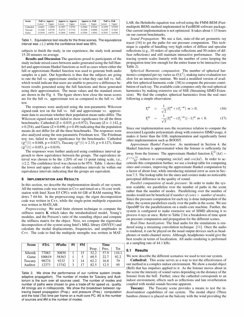
Scene #Tri. #Paths #S #M TimeProp. Pres. Tot

Sibenik 77083 30850 1 15 52.2 57.9 110.1Game 100619 58363 1 5 69.5 22.7 92.2

Tuscany 98274 9232 3 14 62.2 16.8 79Auditor. 12373 13742 3 17 82.5 12.5 95

Table 2. We show the performance of our runtime system (mode-adaptive propagation). The number of modes for Tuscany and Audi-torium is the sum over all sources used. The number of modes andnumber of paths were chosen to give a trade-off for speed vs. quality.All timings are in milliseconds. We show the breakdown between ray-tracing based propagation (Prop.) and pressure (Pres.) computationand the total (Tot) time per frame on a multi-core PC. #S is the numberof sources and #M is the number of modes.

LAB, the Helmholtz equation was solved using the FMM-BEM (Fast-multipole BEM) method implemented in FastBEM software package.Our current implementation is not optimized. It takes about 1-15 hourson our current benchmarks.

Sound Propagation: We use a fast, state-of-the-art geometric raytracer [34] to get the paths for our pressure computation. This tech-nique is capable of handling very high orders of diffuse and specularreflections (e.g., 10 orders of specular reflections and 50 orders of dif-fuse reflections) and still maintain interactive performance. The raytracing system scales linearly with the number of cores keeping thepropagation time low enough for the entire frame to be interactive (seeTable 2).

Spherical Harmonic computation: The number of spherical har-monics computed per ray varies as O(L2), making naive evaluation tooslow for an interactive runtime. We used a modified version of avail-able fast spherical harmonic code [38] to compute the pressure contri-bution of each ray. The available code computes only the real sphericalharmonics by making extensive use of SSE (Streaming SIMD Exten-sion). We find the complex spherical harmonics from the real onesfollowing a simple observation:

Y ml =

1√2(Y m

l + ι Y−ml ) m > 0, (16)

Y ml =

1√2(Y m

l − ι Y−ml )(−1)m m < 0. (17)

Since our implementation uses the recurrence relation to compute theassociated Legendre polynomials along with extensive SIMD usage, itmakes it faster than the GSL implementation and significantly fasterother implementation such as BOOST.

Approximate Hankel Function: As mentioned in Section 4, theHankel function is approximated when the listener is sufficiently faraway from the listener. The approximate Hankel function h(2)l (kd) =

il+1 e−ikd

kd reduces to computing sin(kd) and cos(kd). In order to ac-celerate this computation further, we use a lookup table for computingsines and cosines, improving the approximate Hankel computation bya factor of about four, while introducing minimal error as seen in Sec-tion 7.3. The lookup table for the sines and cosines make no noticeableperceptual difference in the quality of sound.

Parallel computation of mode pressure: In order to make the sys-tem scalable, we parallelize over the number of paths in the scenerather than the number of modes. Parallelizing over the number ofmodes would not be beneficial if number of cores > number of modes.Since the pressure computation for each ray is done independent of theother, the system parallelizes easily over the paths in the scene. We useOpenMP for the parallelization on a multi-core machine. Further, thesystem is configured to make extensive use of SIMD allowing it toprocess 4 rays at once. Refer to Table 2 for a breakdown of time spenton pressure computation and propagation for the different scenes.

Real-Time Auralization: The final audio for the simulations is ren-dered using a streaming convolution technique [11]. Once the audiois rendered, it can be played on the usual output devices such as head-phones or multi-channel stereo. Although, headphones would give thebest results in terms of localization. All audio rendering is performedat a sampling rate of 44.1 kHz.

6.1 ResultsWe now describe the different scenarios we used to test our system.

Cathedral: This scene serves as a way to test the effectiveness ofour method in a complex indoor environment. We show a modal object(Bell) that has impulses applied to it. As the listener moves about inthe scene the intensity of sound varies depending on the distance of thelistener from the bell. Further, since the cathedral corresponds to anindoor environment, effects such as reflections and late reverberationcoupled with modal sounds become apparent.

Tuscany: The Tuscany scene provides a means to test the in-door/outdoor capabilities of our system. The modal object (Threebamboo chimes) is placed on the balcony with the wind providing the

Objeect #Tris Dim. (m) #Modes Freq. Range (Hz) Order

Bell 14600 0.32 20 480 - 2148 13-36Barrel (Auditorium) 7410 0.6 20 397 - 2147 13-37Barrel (Game) 7410 1.03 9 370 - 2334 8-40Chime - Long 3220 0.5 4 780 - 2314 7-19Chime - Medium 3220 0.4 6 1135 - 3958 10-24Chime - Short 3220 0.33 4 1564 - 3495 10-15Bowl 20992 0.35 20 870 - 5945 8-36Drum 7600 0.72 13 477 - 1959 8-28Drum stick 4284 0.23 7 1249 - 3402 7-15Trash can 7936 0.60 5 480 - 1995 11-17

Table 3. We show the characteristics of SPME for different geometriesand materials.

Fig. 5. The order required by the Single-Point multipole generally in-creases with increasing modal frequency. We show the results for theobjects used in our simulations. It is possible for the same modal fre-quency (for different objects) to have different order multipole owing todifference in geometries of these objects. The plot shows the SPME or-der required for approximating the radiation pattern of different objectsas a function of their increasing modal frequencies.

impulses. As the listener goes around the house and moves inside, thepropagated sound of the chimes changes depending on the positionof the listener in the environment. The sound is much less in inten-sity outside owing to most of the propagated sound being lost in theenvironment and increases dramatically when the listener goes in.

Game Scene: This demo showcases the effectiveness of our sys-tem in a game like environment containing, both, an indoor and a semi-outdoor environment. We use a metal barrel as our sounding objectand let the listener interact with it. Initially, the barrel rolls down aflight of stairs in the indoor part of the scene. The collisions withthe stairs serve as input impulses and generate sound in an enclosedenvironment, with effects similar to that in the Cathedral scene. Thelistener then picks up the barrel and rolls it out of the door and followsit. As soon as the barrel exits the door, the environment outside isa semi-outdoor one, the reverberation characteristics change, demon-strating the ability of our system to handle modal sounds with differentenvironments in a complex game scene.

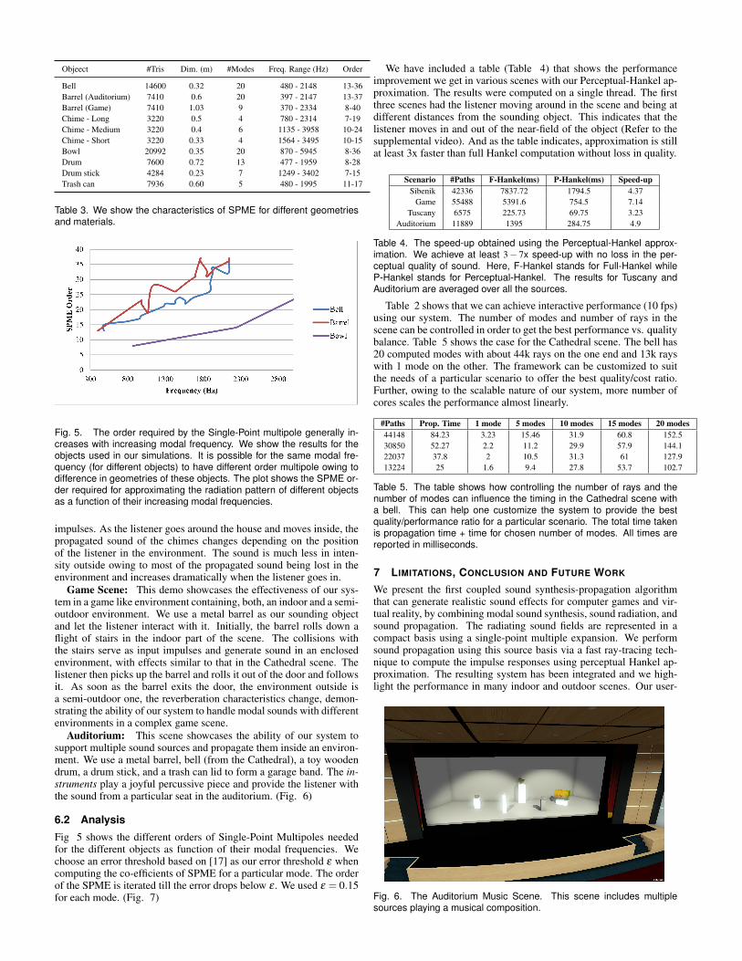
Auditorium: This scene showcases the ability of our system tosupport multiple sound sources and propagate them inside an environ-ment. We use a metal barrel, bell (from the Cathedral), a toy woodendrum, a drum stick, and a trash can lid to form a garage band. The in-struments play a joyful percussive piece and provide the listener withthe sound from a particular seat in the auditorium. (Fig. 6)

6.2 Analysis

Fig 5 shows the different orders of Single-Point Multipoles neededfor the different objects as function of their modal frequencies. Wechoose an error threshold based on [17] as our error threshold ε whencomputing the co-efficients of SPME for a particular mode. The orderof the SPME is iterated till the error drops below ε . We used ε = 0.15for each mode. (Fig. 7)

We have included a table (Table 4) that shows the performanceimprovement we get in various scenes with our Perceptual-Hankel ap-proximation. The results were computed on a single thread. The firstthree scenes had the listener moving around in the scene and being atdifferent distances from the sounding object. This indicates that thelistener moves in and out of the near-field of the object (Refer to thesupplemental video). And as the table indicates, approximation is stillat least 3x faster than full Hankel computation without loss in quality.

Scenario #Paths F-Hankel(ms) P-Hankel(ms) Speed-upSibenik 42336 7837.72 1794.5 4.37

Game 55488 5391.6 754.5 7.14Tuscany 6575 225.73 69.75 3.23

Auditorium 11889 1395 284.75 4.9

Table 4. The speed-up obtained using the Perceptual-Hankel approx-imation. We achieve at least 3− 7x speed-up with no loss in the per-ceptual quality of sound. Here, F-Hankel stands for Full-Hankel whileP-Hankel stands for Perceptual-Hankel. The results for Tuscany andAuditorium are averaged over all the sources.

Table 2 shows that we can achieve interactive performance (10 fps)using our system. The number of modes and number of rays in thescene can be controlled in order to get the best performance vs. qualitybalance. Table 5 shows the case for the Cathedral scene. The bell has20 computed modes with about 44k rays on the one end and 13k rayswith 1 mode on the other. The framework can be customized to suitthe needs of a particular scenario to offer the best quality/cost ratio.Further, owing to the scalable nature of our system, more number ofcores scales the performance almost linearly.

#Paths Prop. Time 1 mode 5 modes 10 modes 15 modes 20 modes44148 84.23 3.23 15.46 31.9 60.8 152.530850 52.27 2.2 11.2 29.9 57.9 144.122037 37.8 2 10.5 31.3 61 127.913224 25 1.6 9.4 27.8 53.7 102.7

Table 5. The table shows how controlling the number of rays and thenumber of modes can influence the timing in the Cathedral scene witha bell. This can help one customize the system to provide the bestquality/performance ratio for a particular scenario. The total time takenis propagation time + time for chosen number of modes. All times arereported in milliseconds.

7 LIMITATIONS, CONCLUSION AND FUTURE WORK

We present the first coupled sound synthesis-propagation algorithmthat can generate realistic sound effects for computer games and vir-tual reality, by combining modal sound synthesis, sound radiation, andsound propagation. The radiating sound fields are represented in acompact basis using a single-point multiple expansion. We performsound propagation using this source basis via a fast ray-tracing tech-nique to compute the impulse responses using perceptual Hankel ap-proximation. The resulting system has been integrated and we high-light the performance in many indoor and outdoor scenes. Our user-

Fig. 6. The Auditorium Music Scene. This scene includes multiplesources playing a musical composition.

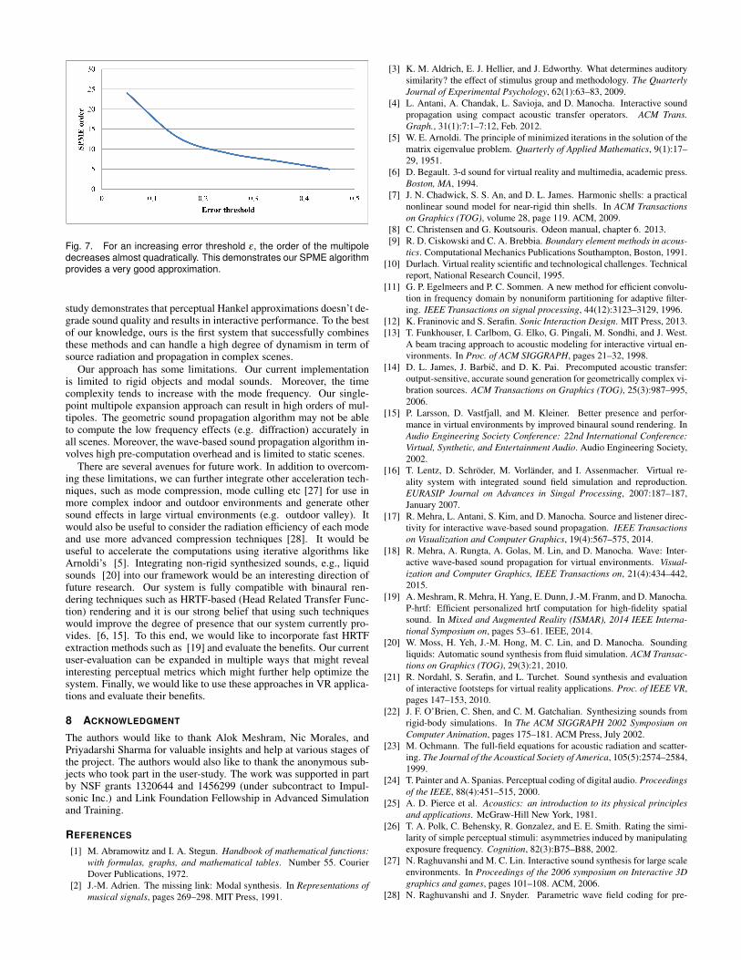
Fig. 7. For an increasing error threshold ε, the order of the multipoledecreases almost quadratically. This demonstrates our SPME algorithmprovides a very good approximation.

study demonstrates that perceptual Hankel approximations doesn’t de-grade sound quality and results in interactive performance. To the bestof our knowledge, ours is the first system that successfully combinesthese methods and can handle a high degree of dynamism in term ofsource radiation and propagation in complex scenes.

Our approach has some limitations. Our current implementationis limited to rigid objects and modal sounds. Moreover, the timecomplexity tends to increase with the mode frequency. Our single-point multipole expansion approach can result in high orders of mul-tipoles. The geometric sound propagation algorithm may not be ableto compute the low frequency effects (e.g. diffraction) accurately inall scenes. Moreover, the wave-based sound propagation algorithm in-volves high pre-computation overhead and is limited to static scenes.

There are several avenues for future work. In addition to overcom-ing these limitations, we can further integrate other acceleration tech-niques, such as mode compression, mode culling etc [27] for use inmore complex indoor and outdoor environments and generate othersound effects in large virtual environments (e.g. outdoor valley). Itwould also be useful to consider the radiation efficiency of each modeand use more advanced compression techniques [28]. It would beuseful to accelerate the computations using iterative algorithms likeArnoldi’s [5]. Integrating non-rigid synthesized sounds, e.g., liquidsounds [20] into our framework would be an interesting direction offuture research. Our system is fully compatible with binaural ren-dering techniques such as HRTF-based (Head Related Transfer Func-tion) rendering and it is our strong belief that using such techniqueswould improve the degree of presence that our system currently pro-vides. [6, 15]. To this end, we would like to incorporate fast HRTFextraction methods such as [19] and evaluate the benefits. Our currentuser-evaluation can be expanded in multiple ways that might revealinteresting perceptual metrics which might further help optimize thesystem. Finally, we would like to use these approaches in VR applica-tions and evaluate their benefits.

8 ACKNOWLEDGMENT

The authors would like to thank Alok Meshram, Nic Morales, andPriyadarshi Sharma for valuable insights and help at various stages ofthe project. The authors would also like to thank the anonymous sub-jects who took part in the user-study. The work was supported in partby NSF grants 1320644 and 1456299 (under subcontract to Impul-sonic Inc.) and Link Foundation Fellowship in Advanced Simulationand Training.

REFERENCES

[1] M. Abramowitz and I. A. Stegun. Handbook of mathematical functions:with formulas, graphs, and mathematical tables. Number 55. CourierDover Publications, 1972.

[2] J.-M. Adrien. The missing link: Modal synthesis. In Representations ofmusical signals, pages 269–298. MIT Press, 1991.

[3] K. M. Aldrich, E. J. Hellier, and J. Edworthy. What determines auditorysimilarity? the effect of stimulus group and methodology. The QuarterlyJournal of Experimental Psychology, 62(1):63–83, 2009.

[4] L. Antani, A. Chandak, L. Savioja, and D. Manocha. Interactive soundpropagation using compact acoustic transfer operators. ACM Trans.Graph., 31(1):7:1–7:12, Feb. 2012.

[5] W. E. Arnoldi. The principle of minimized iterations in the solution of thematrix eigenvalue problem. Quarterly of Applied Mathematics, 9(1):17–29, 1951.

[6] D. Begault. 3-d sound for virtual reality and multimedia, academic press.Boston, MA, 1994.

[7] J. N. Chadwick, S. S. An, and D. L. James. Harmonic shells: a practicalnonlinear sound model for near-rigid thin shells. In ACM Transactionson Graphics (TOG), volume 28, page 119. ACM, 2009.

[8] C. Christensen and G. Koutsouris. Odeon manual, chapter 6. 2013.[9] R. D. Ciskowski and C. A. Brebbia. Boundary element methods in acous-

tics. Computational Mechanics Publications Southampton, Boston, 1991.[10] Durlach. Virtual reality scientific and technological challenges. Technical

report, National Research Council, 1995.[11] G. P. Egelmeers and P. C. Sommen. A new method for efficient convolu-

tion in frequency domain by nonuniform partitioning for adaptive filter-ing. IEEE Transactions on signal processing, 44(12):3123–3129, 1996.

[12] K. Franinovic and S. Serafin. Sonic Interaction Design. MIT Press, 2013.[13] T. Funkhouser, I. Carlbom, G. Elko, G. Pingali, M. Sondhi, and J. West.

A beam tracing approach to acoustic modeling for interactive virtual en-vironments. In Proc. of ACM SIGGRAPH, pages 21–32, 1998.

[14] D. L. James, J. Barbic, and D. K. Pai. Precomputed acoustic transfer:output-sensitive, accurate sound generation for geometrically complex vi-bration sources. ACM Transactions on Graphics (TOG), 25(3):987–995,2006.

[15] P. Larsson, D. Vastfjall, and M. Kleiner. Better presence and perfor-mance in virtual environments by improved binaural sound rendering. InAudio Engineering Society Conference: 22nd International Conference:Virtual, Synthetic, and Entertainment Audio. Audio Engineering Society,2002.

[16] T. Lentz, D. Schroder, M. Vorlander, and I. Assenmacher. Virtual re-ality system with integrated sound field simulation and reproduction.EURASIP Journal on Advances in Singal Processing, 2007:187–187,January 2007.

[17] R. Mehra, L. Antani, S. Kim, and D. Manocha. Source and listener direc-tivity for interactive wave-based sound propagation. IEEE Transactionson Visualization and Computer Graphics, 19(4):567–575, 2014.

[18] R. Mehra, A. Rungta, A. Golas, M. Lin, and D. Manocha. Wave: Inter-active wave-based sound propagation for virtual environments. Visual-ization and Computer Graphics, IEEE Transactions on, 21(4):434–442,2015.

[19] A. Meshram, R. Mehra, H. Yang, E. Dunn, J.-M. Franm, and D. Manocha.P-hrtf: Efficient personalized hrtf computation for high-fidelity spatialsound. In Mixed and Augmented Reality (ISMAR), 2014 IEEE Interna-tional Symposium on, pages 53–61. IEEE, 2014.

[20] W. Moss, H. Yeh, J.-M. Hong, M. C. Lin, and D. Manocha. Soundingliquids: Automatic sound synthesis from fluid simulation. ACM Transac-tions on Graphics (TOG), 29(3):21, 2010.

[21] R. Nordahl, S. Serafin, and L. Turchet. Sound synthesis and evaluationof interactive footsteps for virtual reality applications. Proc. of IEEE VR,pages 147–153, 2010.

[22] J. F. O’Brien, C. Shen, and C. M. Gatchalian. Synthesizing sounds fromrigid-body simulations. In The ACM SIGGRAPH 2002 Symposium onComputer Animation, pages 175–181. ACM Press, July 2002.

[23] M. Ochmann. The full-field equations for acoustic radiation and scatter-ing. The Journal of the Acoustical Society of America, 105(5):2574–2584,1999.

[24] T. Painter and A. Spanias. Perceptual coding of digital audio. Proceedingsof the IEEE, 88(4):451–515, 2000.

[25] A. D. Pierce et al. Acoustics: an introduction to its physical principlesand applications. McGraw-Hill New York, 1981.

[26] T. A. Polk, C. Behensky, R. Gonzalez, and E. E. Smith. Rating the simi-larity of simple perceptual stimuli: asymmetries induced by manipulatingexposure frequency. Cognition, 82(3):B75–B88, 2002.

[27] N. Raghuvanshi and M. C. Lin. Interactive sound synthesis for large scaleenvironments. In Proceedings of the 2006 symposium on Interactive 3Dgraphics and games, pages 101–108. ACM, 2006.

[28] N. Raghuvanshi and J. Snyder. Parametric wave field coding for pre-

computed sound propagation. ACM Transactions on Graphics (TOG),33(4):38, 2014.

[29] Z. Ren, R. Mehra, J. Coposky, and M. C. Lin. Tabletop ensemble: touch-enabled virtual percussion instruments. In Proceedings of the ACM SIG-GRAPH Symposium on Interactive 3D Graphics and Games, pages 7–14.ACM, 2012.

[30] Z. Ren, H. Yeh, R. Klatzky, and M. C. Lin. Auditory perceptionof geometry-invariant material properties. Visualization and ComputerGraphics, IEEE Transactions on, 19(4):557–566, 2013.

[31] Z. Ren, H. Yeh, and M. C. Lin. Synthesizing contact sounds betweentextured models. In Virtual Reality Conference (VR), 2010 IEEE, pages139–146. IEEE, 2010.

[32] D. Rocchesso, S. Serafin, F. Behrendt, N. Bernardini, R. Bresin, G. Eckel,K. Franinovic, T. Hermann, S. Pauletto, P. Susini, and Y. Visell. Sonicinteraction design: Sound, information and experience. Proc. of ACMSIGCHI, pages 3969–3972, 2008.

[33] C. Schissler and D. Manocha. Interactive sound propagation and ren-dering for large multi-source scenes. Technical report, Department ofComputer Science, University of North Carolina at Chapel Hill, 2015.

[34] C. Schissler, R. Mehra, and D. Manocha. High-order diffraction and dif-fuse reflections for interactive sound propagation in large environments.ACM Trans. Graph., 33(4):39:1–39:12, July 2014.

[35] S. Serafin. The Sound OF Friction: Real-Time Models, Playability andMusical Applications. PhD thesis, Stanford University, 2004.

[36] R. D. Shilling and B. Shinn-Cunningham. Virtual auditory displays.Handbook of virtual environment technology, pages 65–92, 2002.

[37] S. Siltanen, T. Lokki, S. Kiminki, and L. Savioja. The room acousticrendering equation. The Journal of the Acoustical Society of America,122(3):1624–1635, September 2007.

[38] P.-P. Sloan. Efficient spherical harmonic evaluation. Journal of ComputerGraphics Techniques (JCGT), 2(2):84–83, September 2013.

[39] F. Steinicke, Y. Visell, J. Campos, and A. Lcuyer. Human Walking inVirtual Environments: Perception, Technology, and Applications. 2015.

[40] M. Taylor, A. Chandak, L. Antani, and D. Manocha. Resound: interactivesound rendering for dynamic virtual environments. In MM ’09: Proceed-ings of the seventeen ACM international conference on Multimedia, pages271–280, New York, NY, USA, 2009. ACM.

[41] E. Terhardt. Calculating virtual pitch. Hearing research, 1(2):155–182,1979.

[42] N. Tsingos, T. Funkhouser, A. Ngan, and I. Carlbom. Modeling acousticsin virtual environments using the uniform theory of diffraction. In Proc.of ACM SIGGRAPH, pages 545–552, 2001.

[43] N. Tsingos, E. Gallo, and G. Drettakis. Perceptual audio renderingof complex virtual environments. ACM Trans. Graph., 23(3):249–258,2004.

[44] L. Turchet. Designing presence for real locomotion in immersive virtualenvironments: an affordance-based experiential approach. Virtual Real-ity, 19(3-4):277–290, 2015.

[45] L. Turchet, S. Spagnol, M. Geronazzo, and F. Avanzini. Localization ofself-generated synthetic footstep sounds on different walked-upon mate-rials through headphones. Virtual Reality, pages 1–16, 2015.

[46] K. van den Doel, P. G. Kry, and D. K. Pai. Foleyautomatic: physically-based sound effects for interactive simulation and animation. In Proc. ofACM SIGGRAPH, pages 537–544, 2001.

[47] Y. Visell, F. Fontana, B. L. Giordano, R. Nordahl, S. Serafin, andR. Bresin. Sound design and perception in walking interactions.67(11):947–959, 2009.

[48] M. Vorlander. Simulation of the transient and steady-state sound propaga-tion in rooms using a new combined ray-tracing/image-source algorithm.The Journal of the Acoustical Society of America, 86(1):172–178, 1989.

[49] D. Young and S. Serafin. Playability evaluation of a virtual bowed stringinstrument. Proc. of Conference on New Interfaces for Musical Expres-sion, pages 104 – 108, 2003.

[50] C. Zheng and D. L. James. Harmonic fluids. ACM Trans. Graph.,28(3):1–12, 2009.

[51] C. Zheng and D. L. James. Toward high-quality modal contact sound.ACM Transactions on Graphics (TOG), 30(4):38, 2011.