sweep mri with algebraic reconstruction
TRANSCRIPT
Sweep MRI with Algebraic Reconstruction
Markus Weiger,1–3* Franciszek Hennel,2 and Klaas P. Pruessmann3
In the recently proposed technique Sweep Imaging with Fou-
rier Transform (SWIFT), frequency-modulated radiofrequency
pulses are used in concert with simultaneous acquisition to
facilitate MRI of samples with very short transverse relaxation
time. In the present work, sweep MRI is reviewed from a
reconstruction perspective and several extensions and modi-
fications of the current methodology are proposed. An algo-
rithm for algebraic image reconstruction is derived from a
comprehensive description of signal formation, including
interleaved radiofrequency transmission and acquisition of ar-
bitrary timing as well as the relevant filtering and decimation
steps along the receiver chain. The new reconstruction
approach readily permits several measures of optimising the
signal sampling strategy as demonstrated in simulations and
imaging experiments. Employing a variety of radiofrequency
pulse envelopes, water and rubber phantoms as well as bone
samples with transverse relaxation time in the order of 500 msec
were imaged at signal bandwidths of up to 96 kHz. Magn Reson
Med 64:1685–1695, 2010. VC 2010 Wiley-Liss, Inc.
Key words: frequency sweep; FM pulses; SWIFT; shorttransverse relaxation time; ultrashort echo time; simultaneousexcitation and acquisition; transmit-receive switching;oversampling
MRI is notoriously difficult to perform in tissues and
organs that give only short-lived NMR signals due to
fast transverse relaxation or dephasing. For instance,
bone, tendons, ligaments, and lung tissue have typical
signal lifetimes in the order of milliseconds or less,
resulting in poor depiction in standard MRI. Notwith-
standing, imaging of these tissues is of great interest in
biological and medical research as well as clinical diag-
nostics, prompting the increasing use of specialized MRI
techniques (1,2).
The primary sensitivity of MRI sequences to signal
decay is typically expressed in terms of the echo time
(TE), which denotes the time that elapses between the
excitation of a signal and its passage through the center
of k-space. TE can be kept especially short with purely
frequency-encoded methods that start acquiring image
signals immediately after excitation without the need for
preceding encoding gradients. The most common
method of this kind is the steady-state three-dimensional
(3D) radial projection technique with ultrashort TE
(UTE) (3). In this method, spatially nonselective radiofre-
quency (RF) excitation is followed by ramping up a
readout gradient and concurrently starting to acquire
data (Fig. 1a). With this approach, the smallest possi-
ble TE is given by a fraction of the RF pulse duration
TRF (one half for symmetric small-flip-angle pulses)
plus the time d that the spectrometer requires for
switching from RF transmission to signal reception. In
addition to keeping TE short, UTE imaging requires com-
plete signal encoding within an acquisition duration AQ in
the order of T*2 to avoid resolution loss due to k-space
apodization (4,5).
Even more efficient but less common is the projection
technique shown in Fig. 1b, in which the readout gradi-
ent is switched on before a hard RF pulse and the free
induction decay (FID) signal is collected as soon as pos-
sible afterward (6–9). In this approach, spatial encoding
starts already during the RF pulse, k ¼ 0 coincides with
the center of the pulse, and TE is hence zero according
to the definition given above. While achieving zero TE,
this approach is still subject to the need to play out an
RF pulse of finite length and to switch from RF transmis-
sion to reception. As a consequence, the data acquisition
starts only after a net dead time D (Fig. 1b) and thus
misses an initial bit of the FID. Correspondingly, the cen-
termost part of k-space is not available for image recon-
struction, requiring special measures to avoid baseline
artifacts (10,11). Importantly, in the zero-TE approach,
the readout gradient does not need to be switched on
and off between successive projections but can be gradu-
ally changed in small steps (7). Similar to the technique
Single-Point Ramped Imaging with T1 Enhancement
(SPRITE) (12), this feature minimizes changes of the Lor-
entz forces on the gradient coils and thus makes the
method virtually silent. Moreover, the zero-TE technique
has a high acquisition duty cycle with only the RF pulse
and the time required for one gradient step as sequence
overhead. However, it is also rather demanding in that
the RF pulse must fully cover the large bandwidth cre-
ated by the gradient. When using a hard pulse, the target
bandwidth translates into the need to make the pulse suffi-
ciently short, which in turn requires high and potentially
excessive RF amplitude (B1).A less B1-intensive approach to large-bandwidth exci-
tation is frequency modulation. RF pulses based on fre-quency sweeps require much less RF amplitude than ahard pulse for achieving a given flip angle across adesired frequency band (13–15). However, to do so, theytake more time. Therefore, simply replacing the hardpulse by a sweep pulse (Fig. 1c) will not work becausesignals excited early during the pulse will be observedtoo late. For imaging with frequency-swept excitationand regular transverse relaxation time (T2), it has beensuggested to solve this issue by gradient or RF refocusingbefore data acquisition (14). Yet for short T2, this
1Bruker BioSpin AG, Faellanden, Switzerland.2Bruker BioSpin MRI GmbH, Ettlingen, Germany.3Institute for Biomedical Engineering, University and ETH Zurich, Zurich,Switzerland.
*Correspondence to: Markus Weiger, Ph.D., Bruker BioSpin AG,Industriestrasse 26, CH-8117 Faellanden, Switzerland. E-mail: [email protected]
Received 20 January 2010; revised 26 April 2010; accepted 28 April 2010.
DOI 10.1002/mrm.22516Published online 14 October 2010 in Wiley Online Library (wileyonlinelibrary.com).
Magnetic Resonance in Medicine 64:1685–1695 (2010)
VC 2010 Wiley-Liss, Inc. 1685
approach is not suitable because it reintroduces a sub-stantial delay between excitation and acquisition, thwart-ing the previous efforts to minimize TE.
The recently proposed technique Sweep Imaging withFourier Transform (SWIFT) (16,17) solves the underlying
timing problem in a radically different way, namely byfrequency-modulated RF excitation with simultaneoussignal acquisition (Fig. 1d). By doing so, it enables zero-TE imaging with large bandwidths at moderate B1 levels.Truly simultaneous excitation and acquisition wouldrequire sufficient decoupling of transmit and receive cir-cuits, which is difficult to achieve in practice. Therefore,current SWIFT implementations rely on interrupting theRF pulse periodically for brief acquisition intervals. Foruseful bandwidths, this approach requires alternatingbetween the transmit and receive states of the spectrome-ter within a few microseconds, which still makes it tech-nically demanding. However, similar modes of operationare known in high-resolution NMR spectroscopy, e.g., forhomonuclear decoupling and are hence available onmost modern NMR systems.
Image reconstruction from data acquired in this man-ner involves undoing the encoding effects of the sweeppulse. In SWIFT, this is accomplished in analogy torelated spectroscopic methods (18,19) by modeling theNMR signal as a time-invariant linear response to the RFpulse. Under this assumption, the signal can be viewedas a convolution of the input function, i.e., the pulse,and the impulse response function, i.e., the free induc-tion decay (FID) that would be received after a hypothet-ical hard-pulse excitation of unit amplitude. On this ba-sis, image reconstruction has been accomplished bydeconvolution and Fourier transform (FT), comple-mented by several further operations (20,21).
In the present work, sweep MRI with simultaneous ex-citation and acquisition is reviewed from a reconstruc-tion perspective, starting from an extended forwarddescription of signal formation and acquisition. The sig-nal model is then used to formulate image reconstructionin a generic algebraic fashion (22). The algebraicapproach is shown to permit robust image formationwith a variety of different sweeping strategies and with-out explicit data correction. Based on closer considera-tions of data collection and image reconstruction, severalmodifications of the acquisition strategy are proposed tooptimise the method’s depiction characteristics and over-all sensitivity (23).
MATERIALS AND METHODS
Acquisition Scheme
Within the scope of this work, sweep MRI is assumed tobe performed in a 3D radial scheme with center-out k-space acquisition like in the original SWIFT implementa-tion (16). First, the parameters of the individual, one-dimensional (1D) readouts shall be defined. To achieve anominal resolution dr with center-out gradient encodingof duration Tenc, the constant readout gradient must beof strength G ¼ 2 �g dr Tencð Þ�1 for nuclei of gyromagneticratio �g ¼ g=2p. Trading off net sensitivity and effectiveresolution, the encoding time is set to a duration in theorder of a representative T*2 value (4,5). For a given fieldof view (FOV), the resulting signal bandwidth isbw ¼ �g G FOV, requiring signal sampling at intervals ofat most dw ¼ 1/bw, which will be referred to as thedwell time in the following.
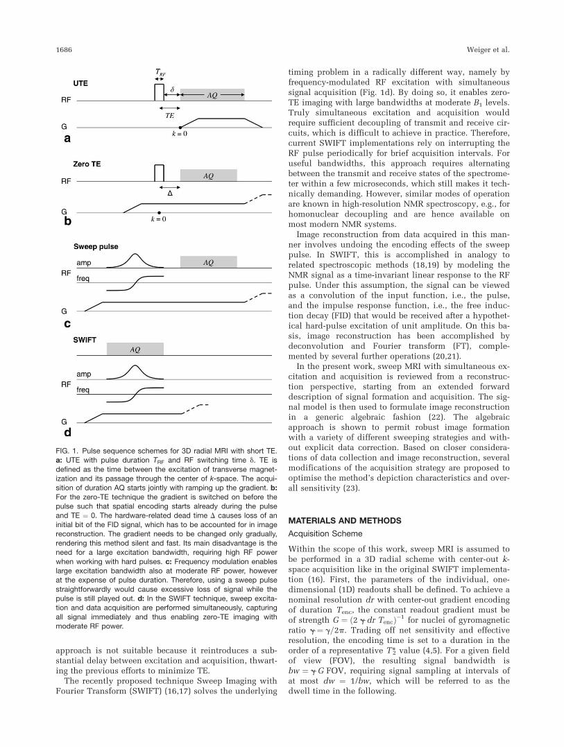
FIG. 1. Pulse sequence schemes for 3D radial MRI with short TE.a: UTE with pulse duration TRF and RF switching time d. TE is
defined as the time between the excitation of transverse magnet-ization and its passage through the center of k-space. The acqui-sition of duration AQ starts jointly with ramping up the gradient. b:For the zero-TE technique the gradient is switched on before thepulse such that spatial encoding starts already during the pulse
and TE ¼ 0. The hardware-related dead time D causes loss of aninitial bit of the FID signal, which has to be accounted for in imagereconstruction. The gradient needs to be changed only gradually,
rendering this method silent and fast. Its main disadvantage is theneed for a large excitation bandwidth, requiring high RF power
when working with hard pulses. c: Frequency modulation enableslarge excitation bandwidth also at moderate RF power, howeverat the expense of pulse duration. Therefore, using a sweep pulse
straightforwardly would cause excessive loss of signal while thepulse is still played out. d: In the SWIFT technique, sweep excita-tion and data acquisition are performed simultaneously, capturing
all signal immediately and thus enabling zero-TE imaging withmoderate RF power.
1686 Weiger et al.
To fully achieve the targeted resolution throughout thesample, transverse magnetization in every part of it mustreach the corresponding spatial modulation while its sig-nal is recorded. To this end, the magnetization that theRF pulse excites last should still be allowed to evolveand be observed for the duration Tenc after the pulse.Also to fully capture the first signals whose gradientencoding begins immediately, data acquisition must starttogether with the RF pulse, leading to the scheme shownin Fig. 2a. For a pulse duration TRF, it prescribes a totalacquisition time of AQ ¼ TRF þ Tenc. By virtue of fre-quency sweeping, any nominal flip angle can be imple-mented irrespective of B1 limits (15). The minimumpulse duration required depends on the sweep widthand flip angle, the pulse shape, and the available RF am-plitude. Including the time TG that is required for adjust-ing the gradient and for inherent gradient spoiling, theminimum repetition time of the described schemeamounts to TR ¼ TRF þ Tenc þ TG.
Figure 2b shows the resulting excitation and acquisi-tion scheme in more detail. During the sweep pulse, RFtransmission and signal sampling are interleaved as indi-cated in the left part of the figure. Dots on the time axisrepresent pulse portions while the ticks indicate signalsamples. The number of samples per dwell time (twoshown) and their timing depend on various factors suchas the time required for transmit-receive switching andthe acquisition bandwidth. The composition of an indi-vidual dwell time dw is shown in Fig. 2c. It contains theactual transmission interval of length rf, the delays d1and d2 for switching from transmission to reception andback, a signal build-up period of duration df caused bydigital filtering, and the effective data acquisition inter-val aq. After completion of the RF pulse, data samplingcan be continued without interruptions to maximize thenet acquisition time (Fig. 2b, right).
Because of the noncontinuity of data acquisition inthis scheme, the role of digital filtering requires closerconsideration. MR signal acquisition commonly includesdigital bandpass filters to enable data decimation with-out loss of net sensitivity (24). Such filters require a cer-tain length of input signal, the filter length, to yield avalid output. As a consequence, when the input signal isgapped due to intermittent RF transmission, the outputsignal first needs to build up after each gap. The dataobtained during the build-up cannot be interpreted assamples of the original MR signal and are hence dis-carded. It is important to note that the issue of the signalbuild-up would be less critical if the MR signal, withoutgapping, were strictly limited to the nominal bandwidthbw. Then the periodical gapping would only lead to fre-quency aliasing outside that band, which could readilybe handled by choosing a long, high-quality band-passfilter. Such a filter would effectively fill the gaps byinterpolation and not require that any of the resultingdata be discarded. However, in sweep acquisition, thesituation is different in that the gapped RF pulse contin-ually generates fresh signal components whose suddenonset spoils the strict band limitation and thus preventsthe interpolation approach.
As a consequence of discarding the data during thesignal build-up, the filter length must not be larger than
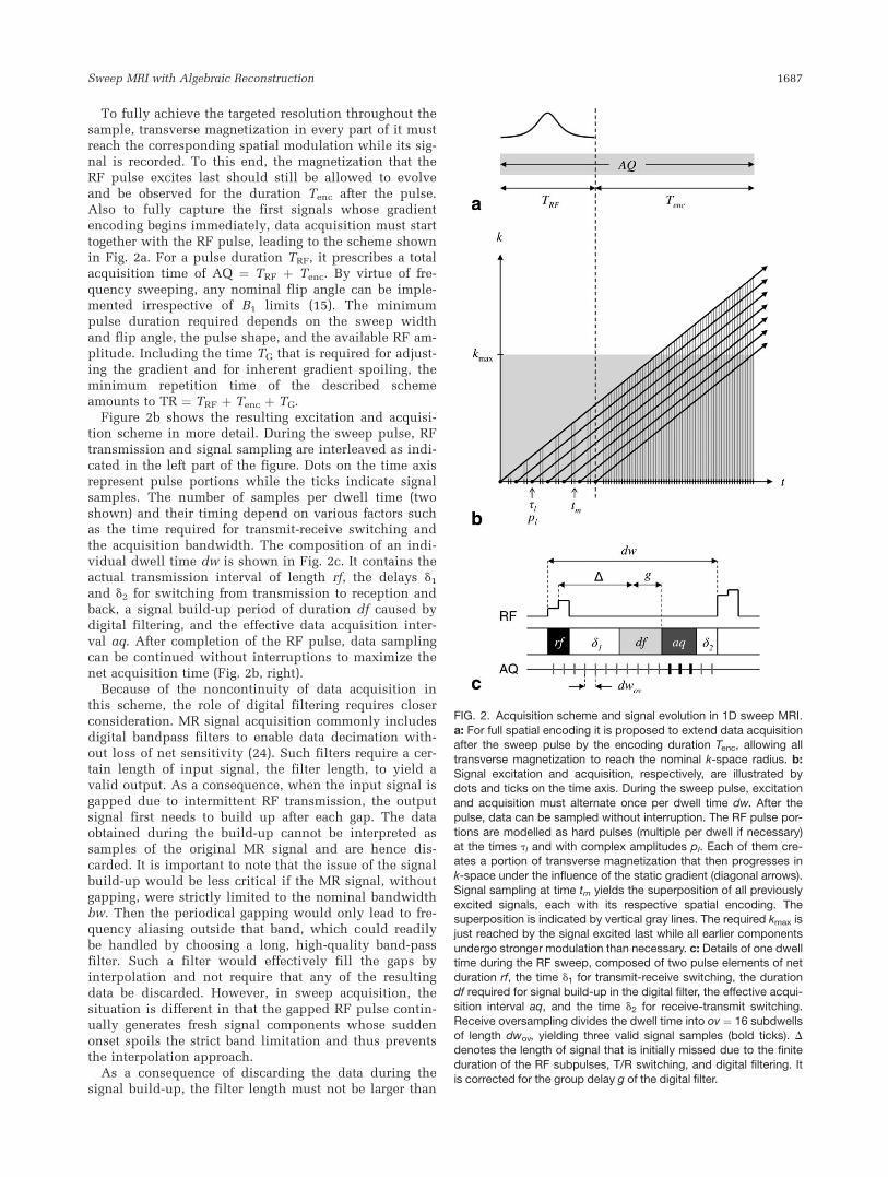
FIG. 2. Acquisition scheme and signal evolution in 1D sweep MRI.
a: For full spatial encoding it is proposed to extend data acquisitionafter the sweep pulse by the encoding duration Tenc, allowing all
transverse magnetization to reach the nominal k-space radius. b:Signal excitation and acquisition, respectively, are illustrated bydots and ticks on the time axis. During the sweep pulse, excitation
and acquisition must alternate once per dwell time dw. After thepulse, data can be sampled without interruption. The RF pulse por-
tions are modelled as hard pulses (multiple per dwell if necessary)at the times tl and with complex amplitudes pl. Each of them cre-ates a portion of transverse magnetization that then progresses in
k-space under the influence of the static gradient (diagonal arrows).Signal sampling at time tm yields the superposition of all previously
excited signals, each with its respective spatial encoding. Thesuperposition is indicated by vertical gray lines. The required kmax isjust reached by the signal excited last while all earlier components
undergo stronger modulation than necessary. c: Details of one dwelltime during the RF sweep, composed of two pulse elements of netduration rf, the time d1 for transmit-receive switching, the duration
df required for signal build-up in the digital filter, the effective acqui-sition interval aq, and the time d2 for receive-transmit switching.
Receive oversampling divides the dwell time into ov ¼ 16 subdwellsof length dwov, yielding three valid signal samples (bold ticks). Ddenotes the length of signal that is initially missed due to the finite
duration of the RF subpulses, T/R switching, and digital filtering. Itis corrected for the group delay g of the digital filter.
Sweep MRI with Algebraic Reconstruction 1687
the acquisition interval aq and should preferably beshorter to maximize the effective acquisition time. Tolimit this loss it is advantageous to use short filters withlarge bandwidth and relatively poor band definition,which in turn require that the eventual sampling band-width be significantly higher than the nominal signalbandwidth bw to prevent loss of net sensitivity. At anoversampling factor ov, ov final data samples of reduceddwell time dwov ¼ dw/ov are obtained per switchingcycle of duration dw as indicated in Fig. 2c. The choiceof ov is governed by a trade-off between net sensitivity,which gradually approaches that of the undecimated dig-ital signal, and the need to keep the resulting amount ofdata in a manageable range.
The center and width sw of the frequency sweep aregenerally chosen such as to cover the band of Larmor fre-quencies present in the object, implying sw ¼ bw. Theregular gaps of the RF pulse, one per dwell time dw,lead to satellites in the pulse spectrum with periodicitybw. With sw ¼ bw, such aliasing can introduce excitationnon-uniformity at the edges of the pulse spectrum (15).Therefore, the choice of frequency and amplitude modu-lation of the sweep pulse is governed by a trade-offbetween pulse duration and spectral uniformity. For thepresent work the class of parameterized hyperbolic se-cant pulses (HSn) defined in Ref. (25) were adopted.Their flip angle can be approximated by the general esti-mate for sweep pulses (13)
u � 2p B1 k h
ffiffiffiffiffiffiffiffiTRF
sw
r½1�
where B1 and sw are given in units of Hz, h ¼ rf/dwdenotes the duty cycle or relative pulse-on time in agapped implementation, and k reflects a shape-depend-ent efficiency, which for an HSn pulse with shape factorn and truncation factor b is given by k ¼ b�1/2n (15). Theless B1-efficient variants with small n yield relatively flatspectral profiles whereas those with larger n lead tomore wiggles in the pulse spectrum.
Signal Evolution
Sweep MRI relies on rather different and arguably morecomplex signal encoding than conventional MRI. With aview to algebraic image reconstruction, the underlyingsignal evolution shall therefore be reconsidered and castinto a linear forward model. Simultaneous excitationand acquisition implies the continued generation of freshtransverse magnetization while the detection of all previ-ously excited coherences is ongoing. The sweep pulsecan be approximated as a series of discrete pulse ele-ments at time points tl, one or multiple per dwell time.Each pulse element must be sufficiently short to describethe pulse modulations with suitable accuracy and to beconsidered a hard pulse with uniform effect across theband of Larmor frequencies that occur in the object. Likefor current SWIFT reconstruction, the resulting trans-verse magnetization is modeled as a linear response tothe train of hard pulses. This is adequate as long as thetotal flip angles induced by the pulse series remain small
at all times, implying that existing transverse magnetiza-tion is not affected by subsequent pulse elements.
Under these prerequisites, the signal evolution duringone sweep acquisition (Fig. 2a) can be viewed as shown inFig. 2b in a representation similar to traditional phase dia-grams (26). At time t1, the first pulse element (representedby a dot) excites the entire object with the complex ampli-tude p1 and the resulting transverse magnetization is sub-sequently encoded by the applied gradient as indicated byan arrow advancing in k-space. The following subpulsescreate similar portions of magnetization, each of the indi-vidual amplitude pl, which evolve in the same way yetwith an increasing time shift. Each tick on the time axis inFig. 2b indicates acquisition of a data point at time tm,receiving the superimposed signals from all magnetizationcomponents that are present at this time as indicated byvertical, gray lines. Note that with oversampling, multiplerelevant samples are taken per dwell time. In the situationshown in Fig. 2c, for instance, the actual acquisition win-dow contains three samples, each of which is assigned itsexact sampling time tm.
According to these considerations, sweep MRI differsfundamentally from conventional MRI in that multiple,differently encoded portions of magnetization exist atthe same time, corresponding to multitple k-space posi-tions that are reached and sampled jointly. The net sig-nal obtained at time tm is given by
sm ¼Xl
pl
ZV
exp i g tm � tlð ÞG � rf g r rð Þ dV ; ½2�
where the sum runs over all l fulfilling tm > tl, Gdenotes the constant gradient vector, r denotes positionin 3D space, r(r) is the available longitudinal magnetiza-tion in the object, and V the volume that it occupies.
The shaded area in Fig. 2b indicates the magnetizationstates that are of actual interest for achieving the selectedresolution dr. It is limited by the corresponding maxi-mum k value of kmax ¼ (2 dr)�1. With the sequence tim-ing described above, the signal that is excited last stilljust reaches this value. All earlier signal components ex-perience stronger eventual modulation.
Algebraic Reconstruction
Algebraic means of image reconstruction were first usedfor other modalities (27,28) but have proven useful alsoin MRI, especially for addressing irregular sampling andnon-Fourier encoding (11,29). The algebraic approach isused here to reconstruct 1D projections from two sweepacquisitions with opposite gradient polarity. To this end,the signal model given by Eq. 2 is first reduced such asto consider only a 1D projection along a given gradientG, which is implemented with opposite polarity (6) intwo successive sweep acquisitions:
s 6ð Þm ¼
Xl
pl
ZV
exp 6ig tm � tlð ÞGrf gr0 rð Þ dr ½3�
where G ¼ |G| is the gradient magnitude, r ¼ (G � r)/Gis the spatial coordinate along the gradient direction,and r0(r) denotes the projection of r(r) onto this
1688 Weiger et al.
dimension. Reconstruction of r0(r) from the measureddata s(6)
m amounts to inverting the linear relationshipdescribed by Eq. 3. To address this problem by means oflinear algebra it is spatially discretized along a regulargrid rj. Let r
0 denote a vector that lists the values of r0(r)at these positions. Likewise, the acquired data areassembled in a joint signal vector s with two stacked par-titions, one for each gradient polarity. Then the discre-tized Eq. 3 can be rewritten in a (complex-valued)matrix-vector form as
s ¼ Er0; ½4�
where the encoding matrix E contains the values that thecoefficients in Eq. 3 assume on the spatial grid:
E6ð Þm;j ¼
Xl
pl
ZV
exp 6ig tm � tlð ÞGrj� �
: ½5�
The two submatrices correspond to the two gradientpolarities and are again stacked to match the structure ofthe signal vector. Because of spatial discretization, Eq. 4is only an approximation of Eq. 3. It is important to note,however, that the discretization can be refined to anylevel of desired accuracy.
Based on these notions, linear image reconstructionamounts to left-multiplying the signal vector by a recon-struction matrix F, yielding an estimate of r0:
r0 ¼ Fs: ½6�
In a broad sense, the reconstruction matrix serves to invertthe encoding represented by E. However, its specific choicestill depends on the target image grid and on the desiredtrade-off between spatial response and signal-to-noise ratio(SNR) (30). Within the scope of the present work, the targetgrid is chosen such as to cover the desired FOV at the nomi-nal resolution dr, yielding N ¼ FOV/dr pixels per 1D pro-jection, and the same grid is used for discretizing theforward model. Strict priority is given to optimising eachpixel’s discretized spatial response. Based on these choices,the reconstruction matrix is calculated as
F ¼ E�; ½7�
where the asterisk indicates the Moore-Penrose pseu-doinverse, which optimises the spatial responses in aleast-squares sense and ensures optimal averaging of anyredundant data components (30). The pseudoinverse iscalculated using a standard algorithm based on singularvalue decomposition (SVD).
Algebraic reconstruction as described above is veryflexible in that the timing and further specifics of anygiven sweep pulse and sampling scheme only need to becorrectly reflected in the encoding matrix (Eq. 5). In par-ticular, interleaved excitation and acquisition, oversam-pling, and data obtained with gradients of opposite signcan be directly incorporated.
Handling Excessive Modulation
It is important to note, however, that the fidelity ofdescribing the signal formation is limited by the chosen
spatial discretization. For instance, modulations beyondkmax as occurring above the shaded area in Fig. 2b can-not be captured on the nominal grid used in this work.In principle, such encoding at higher-than-nominal spa-tial frequencies necessitates finer discretization, which isstraightforward to do per se. However, it complicates theinversion problem in that it will generally be impossibleto still achieve perfect spatial response on the finer grid.It is no longer adequate then to give strict priority to spa-tial response optimisation over noise minimization,requiring an actual trade-off through suitably regularizedinversion (31,32). While this path is promising toexplore, to keep the initial demonstrations simple, thepresent work relies on a mild assumption instead. Usingonly nominal grids as described above, excessivelymodulated magnetization was simply neglected by limit-ing the sum in Eq. 5 to terms with 0 < tm � tl � Tenc. Bydoing so, it is effectively assumed that inherent spoilingand T*2 decay render such magnetization negligible, anassumption that appears justified by the experimentalresults presented later in this work.
3D Reconstruction
Like in common radial MRI, for 3D sweep imaging alarge number of approximately evenly distributed 1Dprojections is obtained by sweeps with different gradientdirections. Each of them is processed according to Eq. 6using the same reconstruction matrix F that is calculatedand stored once initially. A range of established methodsexist for reconstructing 3D image data from the projec-tions, including filtered back-projection and Fourierinterpolation. In the present work the latter approachwas used, consisting of initial inverse FT of each 1D pro-jection, followed by density-corrected gridding in 3Dk-space, 3D forward FT, and apodization correction (33).
Experimental
Imaging experiments were conducted at 4.7 T using aBruker BioSpec animal MRI scanner (Bruker BioSpin,Ettlingen, Germany) equipped with an Avance AVIIIconsole.
Many of the materials commonly used for building RFcoils emit proton signal with T2 on the order of a fewtens of microseconds. While not seen with conventionalMRI methods, such signal contaminates images obtainedwith short-T2 techniques and typically appears blurredas it decays before spatial encoding is completed. Inaddition, aliasing artifacts can occur when the materialis located outside the FOV or even outside the unambig-uous range of the gradient field. Therefore, RF transmis-sion and reception were performed with a special quad-rature birdcage coil, in which all parts giving significantproton signal were replaced by either glass or TeflonVR .The maximum available RF amplitude of the coil wasBmax1 ¼ 9.73 kHz.Sweep MRI acquisition was implemented with switch-
ing times of d1 ¼ 3.5 msec and d2 ¼ 1.5 msec. To simplifythe initial implementation, acquisition gapping was con-tinued after completion of the sweep pulse, i.e., only thecorresponding fraction of the data samples shown in Fig.
Sweep MRI with Algebraic Reconstruction 1689
2b were actually considered. Unless stated otherwise thebandwidth was bw ¼ 83.3 kHz, corresponding to thedwell time dw ¼ 12 msec. Oversampling by a factor of ov¼ 16 resulted in an actual data bandwidth of 1.33 MHz,corresponding to a sub-dwell time of dwov ¼ 0.75 msec.The resulting division of the dwell time is illustrated inFig. 2c. Initially, 1.5 msec of each dwell were used forRF transmission, played out as two successive portionsof 0.75 msec each and amounting to a pulse duty cycle ofh ¼ 0.125. A short, symmetric digital filter was selectedon the MRI system’s digital receiver unit (DRUTM). It hada length of ndf ¼ 5 in terms of output dwells, resultingin a group delay of g ¼ ndf dwov/2 ¼ 1.875 msec and asignal build-up duration of df ¼ (ndf � 1) dwov ¼ 3.0msec. Once the filter was filled, three out of 16 subdwellsyielded valid signals, corresponding to the effective ac-quisition interval aq ¼ 2.25 msec. Overall, RF transmis-
sion, T/R switching, and signal build-up in the filtercause a dead time that elapses until freshly excited mag-netization is first observed. Neglecting the small timingdifference between multiple pulse portions within rf,this dead time amounted to D ¼ rf/2 þ d1 þ df � g ¼5.375 msec. For some experiments, the bandwidth wasset to the practical maximum of bw ¼ 96.2 kHz, reducingthe dwell time to dw ¼ 10.4 msec and yielding two validdata points per dwell.
Further parameters were N ¼ 128, Tenc ¼ 768 or 666msec, FOV ¼ 7.0 or 8.6 cm, pulse repetition time ¼ 7.5–25 msec, y ¼ 4.7–10.5�, and 51,896 gradient directionsincluding positive and negative polarity. No averagingwas performed. The length of the HS sweep pulse, TRF,was set to values between Tenc/4 and Tenc to reflect dif-ferent degrees of B1 limitation. Before starting the acqui-sition, the magnetization was driven into steady state byan appropriate number of dummy scans with reversedgradient order.
Sweep MRI was performed in four different samples.A glass sphere of 5 cm in diameter was filled with dis-tilled water of T*2 � 3 sec to study imaging performancewithout any k-space apodization effects due to signaldecay. To demonstrate short-T2 capability, a phantomwas composed of rubbers (erasers) and pieces of rubbertube with T*2 � 400 msec. Finally, two calf-bone sampleswere used, sample A with T*2 � 600 msec and sample Bwith two components of T*2 � 230 and 50 msec.
Algebraic reconstruction was conducted in MATLABVR ,taking �150 sec for building E, 1 sec for obtaining F byinversion, and 1 msec for reconstructing a 1D projectionby application of F to raw data, with substantial roomfor speed improvement, particularly in the first step. 3Dreconstruction was performed with the gridding routinesavailable on the imaging system.
RESULTS
Simulations
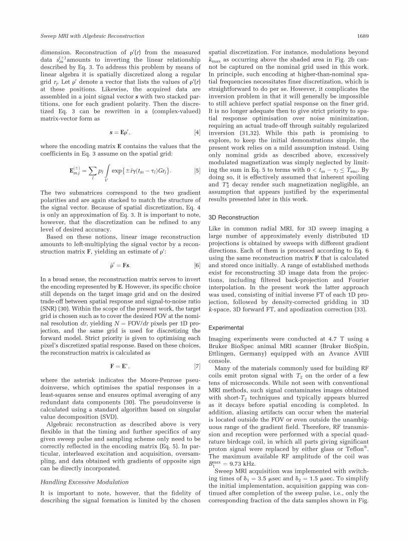
Figure 3 shows an initial set of 1D simulations that wereperformed to verify the benefit of continuing data acqui-sition after completing the sweep pulse. The original 1Dobject was a real-valued rectangle filling 80% of the FOV(Fig. 3a). Targeting image vectors with N ¼ 128, data ac-quisition was simulated with an original object of eight-fold higher spatial resolution to capture spatial responseimperfections. The k-space representation of this objectwas obtained by FT. After limiting it to the nominal ac-quisition range for N ¼ 128, standard FT reconstructionyielded the image shown in Fig. 3b, exhibiting commonGibbs ringing in the real part due to k-space truncation.The full k-space data were then used to simulate differ-ent variants of sweep MRI schemes via Eq. 3, all relyingon two acquisitions with opposing gradients obtainedwith the HS1 pulse without gapping or oversamplingand full-Fourier reconstruction. A very small amount ofGaussian white noise was added (standard deviation ¼10�6 times the maximum signal magnitude) to revealpotential ill-conditioning of the reconstruction problem.
In a first-sweep example, the signal acquisition wasassumed to end jointly with the RF pulse according toFig. 1d. Algebraic reconstruction from the resulting data
FIG. 3. Benefit of extended acquisition, shown by 1D simulations.
a: Original rectangular object represented at eight times higher re-solution than targeted by the simulated imaging experiments. b:Standard Fourier imaging with common Gibbs ringing due to finite
k-space coverage. c: Result of algebraic reconstruction from dataobtained with sweep MRI and signal acquisition only during the
RF pulse (cf. Fig 1d). The result is dominated by massively ampli-fied noise, indicating ill-conditioning of straightforward inversion.d: Regularization by truncated SVD suppresses excessively noisy
image components and largely recovers the object from the samedata. However, it also reveals missing image components by
increased ringing and oscillations of the imaginary part. e: Extend-ing data acquisition as shown in Fig. 2a permitted robust alge-braic reconstruction without regularization. Full spatial encoding is
reflected by virtually exact reproduction of the standard-Fourierresult in (b).
1690 Weiger et al.
failed due to ill-conditioning of the inversion in Eq. 7, asreflected by excessive noise amplification (Fig. 3c). Theconditioning problem is attributed to incomplete spatialencoding of signals generated late during the pulse. Itcan be addressed by regularization, i.e., by reducing theinfluence of small singular values on the inverse prob-
lem. Basic regularization was implemented by truncatedSVD, limiting the condition number to 104. As seen inFig. 3d, the regularized reconstruction largely recoveredthe object, but yielded stronger ringing than in the stand-ard Fourier case and significant oscillations also of theimaginary part. Both effects are attributed to criticallysmall singular values of the encoding matrix, reflectingthat the corresponding image components were scarcelyencoded. Finally, the newly proposed scheme with con-tinued acquisition after the sweep pulse (AQ ¼ TRF þTenc) was simulated. In this case, algebraic reconstruc-tion without regularization (condition number ¼ 1.9)yielded a profile with only minimally increased ringingand no alteration of the imaginary part (Fig. 3e).
Measurements
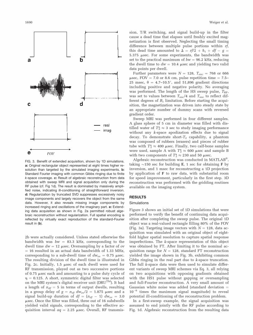
In a first set of experiments, sweep imaging was per-formed in the water phantom with FOV ¼ 7 cm, pulserepetition time ¼ 25 msec, and y ¼ 4.7�. A first data setwas acquired with a HS1 pulse with TRF ¼ Tenc, b ¼ 5,and k ¼ 0.45, requiring B1 ¼ 2.43 kHz according to Eq.1. Figure 4 shows the results of a sample 1D projection,where the raw data (real part) obtained from one readoutas plotted in Fig. 4a show the typical behavior of thetransverse magnetization in a sweep MRI acquisition.The signal in the first half reflects the envelope of thesweep pulse, the rapid phase changes associated withthe frequency sweep, and the gapped acquisitionscheme. The zoomed detail in Fig. 4b illustrates the sig-nal behavior during the pulse for about two dwell timescorresponding to the timing in Fig. 2c. It shows blankingof the receive channel during RF transmission and theswitching time d1, signal build-up as the digital filtergradually fills, the subsequent valid data samples, andtapering of the filtered signal during the next switchingoperation (d2). Reconstruction from data acquired withpositive and negative gradient polarity and correction forthe global spectrometer phase (not required for magni-tude images) yield a projection of the sphere, which ispredominantly real-valued and exhibits only a very smallimaginary part. Initial signal gaps, as present in theunderlying data, have previously been found to entailbaseline artefacts (11). Therefore, it is noteworthy thatalgebraic reconstruction yielded a virtually flat baselinewithout explicit correction.
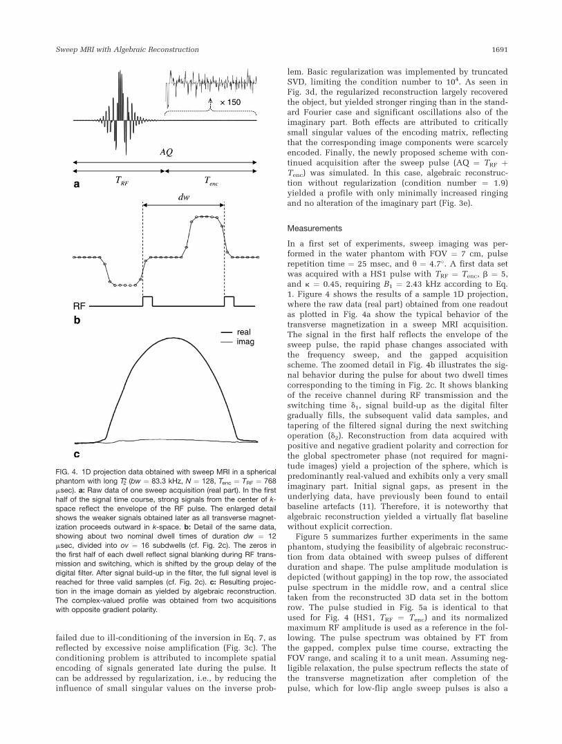
Figure 5 summarizes further experiments in the samephantom, studying the feasibility of algebraic reconstruc-tion from data obtained with sweep pulses of differentduration and shape. The pulse amplitude modulation isdepicted (without gapping) in the top row, the associatedpulse spectrum in the middle row, and a central slicetaken from the reconstructed 3D data set in the bottomrow. The pulse studied in Fig. 5a is identical to thatused for Fig. 4 (HS1, TRF ¼ Tenc) and its normalizedmaximum RF amplitude is used as a reference in the fol-lowing. The pulse spectrum was obtained by FT fromthe gapped, complex pulse time course, extracting theFOV range, and scaling it to a unit mean. Assuming neg-ligible relaxation, the pulse spectrum reflects the state ofthe transverse magnetization after completion of thepulse, which for low-flip angle sweep pulses is also a
FIG. 4. 1D projection data obtained with sweep MRI in a sphericalphantom with long T*2 (bw ¼ 83.3 kHz, N ¼ 128, Tenc ¼ TRF ¼ 768msec). a: Raw data of one sweep acquisition (real part). In the first
half of the signal time course, strong signals from the center of k-space reflect the envelope of the RF pulse. The enlarged detail
shows the weaker signals obtained later as all transverse magnet-ization proceeds outward in k-space. b: Detail of the same data,showing about two nominal dwell times of duration dw ¼ 12
msec, divided into ov ¼ 16 subdwells (cf. Fig. 2c). The zeros inthe first half of each dwell reflect signal blanking during RF trans-mission and switching, which is shifted by the group delay of the
digital filter. After signal build-up in the filter, the full signal level isreached for three valid samples (cf. Fig. 2c). c: Resulting projec-
tion in the image domain as yielded by algebraic reconstruction.The complex-valued profile was obtained from two acquisitionswith opposite gradient polarity.
Sweep MRI with Algebraic Reconstruction 1691
good estimate of the maximum transverse magnetizationavailable during the pulse. The pulse spectrum in Fig.5a shows a broad, flat, central region and some wigglesat the edges, which are caused by aliasing that is associ-ated with the gapping. The corresponding image is ofgood quality. It is a uniform representation of the homo-geneous sphere, showing some detail of the filler neck, aglimpse of the short-T2 rubber cap, but no conspicuousartefacts. For Fig. 5b, a HS5 pulse was used with thesame duration but reduced B1 ¼ 1.28 kHz to compensatefor the better efficiency as reflected by the larger valueof k ¼ 0.85. As expected, the pulse spectrum showssomewhat increased distortions but the resulting imagequality is practically identical to that obtained with theless efficient HS1 pulse at almost twice the B1 ampli-tude. For Fig. 5c, the acquisition scheme was modifiedby halving the duration of the HS1 pulse, thus requiringan increased amplitude of B1 ¼ 3.44 kHz, and resultingin a pulse spectrum with reduced edge definition butstill yielding a practically identical image free of arte-facts. Finally, the shorter HS1 pulse was implemented
in a simpler fashion, allowing only one complex valueper dwell, which resulted in a more pronouncedstaircase modulation. Figure 5d shows that this lead tofurther perturbation of the pulse spectrum but againdid not affect the feasibility of algebraic imagereconstruction.
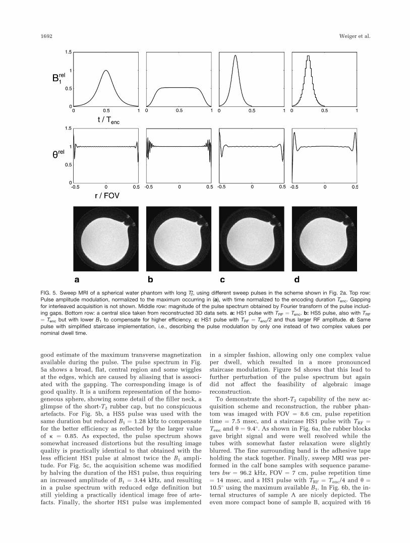
To demonstrate the short-T2 capability of the new ac-quisition scheme and reconstruction, the rubber phan-tom was imaged with FOV ¼ 8.6 cm, pulse repetitiontime ¼ 7.5 msec, and a staircase HS1 pulse with TRF ¼Tenc and y ¼ 9.4�. As shown in Fig. 6a, the rubber blocksgave bright signal and were well resolved while thetubes with somewhat faster relaxation were slightlyblurred. The fine surrounding band is the adhesive tapeholding the stack together. Finally, sweep MRI was per-formed in the calf bone samples with sequence parame-ters bw ¼ 96.2 kHz, FOV ¼ 7 cm, pulse repetition time¼ 14 msec, and a HS1 pulse with TRF ¼ Tenc/4 and y ¼10.5� using the maximum available B1. In Fig. 6b, the in-ternal structures of sample A are nicely depicted. Theeven more compact bone of sample B, acquired with 16
FIG. 5. Sweep MRI of a spherical water phantom with long T*2, using different sweep pulses in the scheme shown in Fig. 2a. Top row:Pulse amplitude modulation, normalized to the maximum occurring in (a), with time normalized to the encoding duration Tenc. Gapping
for interleaved acquisition is not shown. Middle row: magnitude of the pulse spectrum obtained by Fourier transform of the pulse includ-ing gaps. Bottom row: a central slice taken from reconstructed 3D data sets. a: HS1 pulse with TRF ¼ Tenc. b: HS5 pulse, also with TRF¼ Tenc but with lower B1 to compensate for higher efficiency. c: HS1 pulse with TRF ¼ Tenc/2 and thus larger RF amplitude. d: Same
pulse with simplified staircase implementation, i.e., describing the pulse modulation by only one instead of two complex values pernominal dwell time.
1692 Weiger et al.
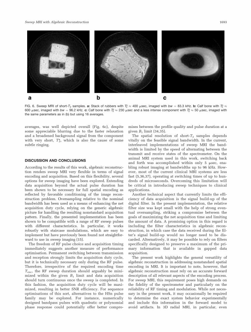
averages, was well depicted overall (Fig. 6c), despitesome appreciable blurring due to the faster relaxationand a broadened background signal from the componentwith very short, T*2, which is also the cause of somesubtle ringing.
DISCUSSION AND CONCLUSIONS
According to the results of this work, algebraic reconstruc-tion renders sweep MRI very flexible in terms of signalencoding and acquisition. Based on this flexibility, severaloptions for sweep imaging have been explored. Extendingdata acquisition beyond the actual pulse duration hasbeen shown to be necessary for full spatial encoding asreflected by favorable conditioning of the image recon-struction problem. Oversampling relative to the nominalbandwidth has been used as a means of enhancing the netacquisition duty cycle, relying on the generic algebraicpicture for handling the resulting nonstandard acquisitionpattern. Finally, the presented implementation has beenshown to be compatible with a range of RF sweep pulseswith different characteristics. In particular, it worksrobustly with staircase modulations, which are easy toimplement but have previously been found not straightfor-ward to use in sweep imaging (15).
The freedom of RF pulse choice and acquisition timingimmediately suggests another measure of performanceoptimisation. Permanent switching between transmissionand reception strongly limits the acquisition duty cycle,but it is technically necessary only during the RF pulse.Therefore, irrespective of the required encoding timeTenc, the RF sweep duration should arguably be mini-mized within the given B1 limit and data acquisitionshould turn continuous once the sweep is completed. Inthis fashion, the acquisition duty cycle will be maxi-mized, resulting in better SNR efficiency. For sequenceoptimisations of this sort, alternatives to the HSn pulsefamily may be explored. For instance, numericallydesigned bandpass pulses with quadratic or polynomialphase response could potentially offer better compro-
mises between the profile quality and pulse duration at agiven B1 limit (34,35).
The spatial resolution of short-T2 samples dependsvitally on the feasible signal bandwidth. In the current,interleaved implementations of sweep MRI the band-width is limited by the speed of alternating between thetransmit and receive states of the spectrometer. On theanimal MRI system used in this work, switching backand forth was accomplished within only 5 msec, ena-bling robust imaging at bandwidths up to 96 kHz. How-ever, most of the current clinical MRI systems are lessfast (5,36,37), operating at switching times of up to hun-dreds of microseconds. Overcoming this limitation willbe critical in introducing sweep techniques to clinicalapplications.
Another technical aspect that currently limits the effi-ciency of data acquisition is the signal build-up of thedigital filter. In the present implementation, the relativefilter size was kept small with the help of strong even-tual oversampling, striking a compromise between thegoals of maximizing the net acquisition time and limitingthe amount of data. A promising option in this regard isincluding the filter characteristics in algebraic recon-struction, in which case the data received during the fil-ter’s signal build-up would no longer need to be dis-carded. Alternatively, it may be possible to rely on filtersspecifically designed to preserve a maximum of the pri-mary information that is available in gapped dataacquisition.
The present work highlights the general versatility ofalgebraic reconstruction in addressing nonstandard spatialencoding in MRI. It is important to note, however, thatalgebraic reconstruction must rely on an accurate forwarddescription of all relevant aspects of the encoding process.For sweep MRI, this requirement poses high demands onthe fidelity of the spectrometer and particularly on thereliability of RF timing and modulation. While not neces-sary in the present work, it may occasionally be requiredto determine the exact system behavior experimentallyand include this information in the forward model toavoid artifacts. In 3D radial MRI, in particular, even
FIG. 6. Sweep MRI of short-T2 samples. a: Stack of rubbers with T*2 � 400 msec, imaged with bw ¼ 83.3 kHz. b: Calf bone with T*2 �600 msec, imaged with bw ¼ 96.2 kHz. c: Calf bone with T*2 � 230 msec and a less intense component with T*2 � 50 msec, imaged with
the same parameters as in (b) but using 16 averages.
Sweep MRI with Algebraic Reconstruction 1693
minute defects, when repeated in the individual projec-tions, may cause significant errors in the final 3D image,e.g., the so-called ‘‘bulls-eye’’ artifacts (21). Further aspectsthat could be incorporated in algebraic reconstructioninclude time-varying gradients, encoding fields that arenon-linear in space, static field inhomogeneity, higherorder coherences, acquisition with a coil array, and encod-ing by means of coil sensitivity. However, greater complex-ity of the forward model and algebraic reconstruction inmore than 1D may prevent straightforward inversion of theencoding matrix, necessitating iterative algorithms (38).
As discussed in the Introduction, in short-T2 techni-ques, all variants of sweep MRI compete with UTE andzero-TE imaging with hard pulse excitation. Arguably, itis most closely related to the latter method, with funda-mental differences only in terms of signal excitation and,of course, its synchrony with data acquisition. A uniqueadvantage of sweep MRI is the ability to reach anydesired nominal flip angle at limited B1, which is essen-tial for obtaining optimum SNR and, in steady-statesequences, creating T1 contrast. This property renderssweep imaging particularly interesting for human MRI athigh field, where B1 is often limited to about 1 kHz orless. On the other hand, hard-pulse excitation, whenpossible, offers superior acquisition duty cycle and issimpler to implement. An actual comparison of sweep-and hard-pulse excitation in zero-TE MRI is beyond thescope of this article and will need to include, in particu-lar, a detailed analysis of SNR efficiency. It is notewor-thy, however, that the SNR analysis will benefit from thelinear-algebraic reconstruction context because it readilypermits formal SNR calculations (30).
Apart from its practical potential and implications,sweep imaging is also of great interest from a conceptualpoint of view. Compared to standard MRI, it stands outby the fact that it relies on multiple portions of trans-verse magnetization that concurrently exhibit differentspatial encoding. In doing so, it effectively samples k-space at many positions simultaneously and thus reachesfundamentally beyond the common notion of samplingk-space along a unique trajectory (39). In a sense, thesame could be said of several previous techniques, suchas BURST (40) or PRESTO (41), in which multiple por-tions of transverse magnetization also coexist at very dif-ferent k-space positions. Arguably, it could even be saidof common imaging sequences with gradient spoiling.However, in these techniques, it is generally assumedthat signals from all but one k-space position can beneglected due to excessive modulation. This is indeedfundamentally different in sweep MRI, where a largenumber of coherences actually coexist at different posi-tions within the sensitive k-space range. As a conse-quence, sweep MRI requires more general signal modelsand reconstruction strategies such as those discussed inthis work.
ACKNOWLEDGMENTS
Dr. Gerhard Eber from Bruker BioSpin GmbH, Rheinstet-ten, Germany, is acknowledged for supporting the imple-mentation of sweep MRI acquisition. The authors alsothank Martin Tabbert from Bruker BioSpin MRI GmbH,
Ettlingen, Germany, for providing the proton-free RFcoil. Finally, we owe Michael Schenkel from Bruker Bio-Spin AG, Switzerland, for giving us detailed insight intothe field of digital filters and receivers.
REFERENCES
1. Gatehouse PD, Bydder M. Magnetic resonance imaging of short T2
components in tissue. Clin Radiol 2003;58; 1–19.
2. Eichinger M, Tetzlaff R, Puderbach M, Woodhouse N, Kauczor HU.
Proton magnetic resonance imaging for assessment of lung function
and respiratory dynamics. Eur J Radiol 2007;64; 329–334.
3. Glover GH, Pauly JM, Bradshaw KM. Boron-11 imaging with a three-
dimensional reconstruction method. J Magn Reson Imaging 1992;2:
47–52.
4. Callaghan PT, Eccles CD. Sensitivity and resolution in NMR imaging.
J Magn Reson 1987;71:426–445.
5. Rahmer J, Bornert P, Groen J, Bos C. Three-dimensional radial ultra-
short echo-time imaging with T2 adapted sampling. Magn Reson
Med 2006;55:1075–1082.
6. Hafner S. Fast imaging in liquids and solids with the back-projection
low angle shot (BLAST) technique. Magn Reson Imaging 1994;12:
1047–1051.
7. Madio DP, Lowe IJ. Ultra-fast imaging using low flip angles and
FIDs. Magn Reson Med 1995;34:525–529.
8. Kuethe DO, Caprihan A, Fukushima E, Waggoner RA. Imaging lungs
using inert fluorinated gases. Magn Reson Med 1998;39:85–88.
9. Wu Y, Ackerman JL, Chesler DA, Li J, Neer RM, Wang J, Glimcher
MJ. Evaluation of bone mineral density using three-dimensional solid
state phosphorus-31 NMR projection imaging. Calcif Tissue Int 1998;
62:512–518.
10. Zhu G, Torchia DA, Bax A. Discrete Fourier transformation of NMR
signals. The relationship between sampling delay time and spectral
baseline. J Magn Reson A 1993;105:219–222.
11. Kuethe DO, Transforming NMR data despite missing points. J Magn
Reson 1999;139:18–25.
12. Balcom BJ, MacGregor RP, Beyea SD, Green DP, Armstrong RL,
Bremner TW. Single-point ramped imaging with T1 enhancement
(SPRITE). J Magn Reson A 1996;123:131–134.
13. Kunz DW. Use of frequency-modulated radiofrequency pulses in MR
imaging experiments. Magn Reson Med 1986;3:377–384.
14. Pipe JG. Spatial encoding and reconstruction in MRI with quadratic
phase profiles. Magn Reson Med 1995;33:24–33.
15. Idiyatullin D, Corum C, Moeller S, Garwood M. Gapped pulses for
frequency-swept MRI. J Magn Reson 2008;193:267–273.
16. Idiyatullin D, Corum C, Park JY, Garwood M. Fast and quiet MRI
using a swept radiofrequency, J Magn Reson 2006;181:342–349.
17. Corum CA, Idiyatullin D, Moeller S, Garwood M. Progress in 3d
Imaging at 4 T with SWIFT. In: Proceedings of International Society
of Magnetic Resonance in Medicine, Berlin, 2007. p 1330.
18. Dadok J, Sprecher RF. Correlation NMR spectroscopy. J Magn Reson
1974;13:243–248.
19. Gupta RK, Ferretti JA, Becker ED. Rapid scan Fourier transform NMR
spectroscopy. J Magn Reson 1974;13:275–290.
20. Corum CA, Moeller S, Idiyatullin D, Garwood M. Signal processing
and image reconstruction for SWIFT. In: Proceedings of International
Society of Magnetic Resonance in Medicine, Berlin, 2007. p 1669.
21. Moeller S, Corum CA, Idiyatullin D, Chamberlain R, Garwood M.
Correction of RF pulse distortions in radial imaging using SWIFT, In:
Proceedings of International Society of Magnetic Resonance in Medi-
cine, Toronto, 2008. p. 229.
22. Weiger M, Pruessmann KP, Hennel F. Reconstruction strategies for
MRI with simultaneous excitation and acquisition. In: Proceedings of
International Society of Magnetic Resonance in Medicine, Honolulu,
2009. p. 557.
23. Weiger M, Pruessmann KP, Tabbert M, Hennel F. Sampling strategies
for MRI with simultaneous excitation and acquisition. In: Proceed-
ings of International Society of Magnetic Resonance in Medicine,
Honolulu, 2009. p. 252.
24. Moskau D. Application of real time digital filters in NMR spectros-
copy. Concepts Magn Reson 2002;15:164–176.
25. Tannus A, Garwood M. Improved performance of frequency-swept
pulses using offset-independent adiabaticity. J Magn Reson A 1996;
120:133–137.
1694 Weiger et al.
26. Hennig J. Multiecho imaging sequences with low refocusing flip
angles. J Magn Reson 1988;78:397–407.
27. Gordon R, Bender R, Herman GT. Algebraic reconstruction techni-
ques (ART) for three-dimensional electron microscopy and x-ray
photography. J Theor Biol 1970;29:471–481.
28. Andersen AH. Algebraic reconstruction in CT from limited views.
IEEE Trans Med Imaging 1989;8:50–55.
29. Pruessmann KP, Weiger M, Scheidegger MB, Boesiger P. SENSE: sen-
sitivity encoding for fast MRI. Magn Reson Med 1999;42:952–962.
30. Pruessmann KP. Encoding and reconstruction in parallel MRI. NMR
Biomed 2006;19:288–299.
31. Lin FH, Kwong KK, Belliveau JW, Wald LL. Parallel imaging recon-
struction using automatic regularization. Magn Reson Med 2004;51:
559–567.
32. Sanchez-Gonzalez J, Tsao J, Dydak U, Desco M, Boesiger P, Pruess-
mann KP. Minimum-norm reconstruction for sensitivity-encoded
magnetic resonance spectroscopic imaging. Magn Reson Med 2006;
55:287–295.
33. Jackson JI, Meyer CH, Nishimura DG, Macovski A. Selection of a con-
volution function for Fourier inversion using gridding. IEEE Trans
Med Imaging 1991;10:473–478.
34. Schulte RF, Tsao J, Boesiger P, Pruessmann KP. Equi-ripple design of
quadratic-phase RF pulses. J Magn Reson 2004;166:111–122.
35. Schulte RF, Henning A, Tsao J, Boesiger P, Pruessmann KP. Design
of broadband RF pulses with polynomial-phase response. J Magn
Reson 2007;186:167–175.
36. Brittain JH, Shankaranarayanan A, Ramanan V, Shimakawa A, Cun-
ningham CH, Hinks S, Francis R, Turner R, Johnson JW, Nayak KS,
Tan S, Pauly JM, Bydder GM. Ultrashort TE imaging with single-digit
(8 ls) TE. In: Proceedings of the 12th Annual Meeting of ISMRM,
Kyoto, Japan, 2004. p. 629.
37. Valette J, Moeller S, Idiyatullin D, Corum C, Le Bihan D, Garwood
M, Lethimonnier F. Implementation of SWIFT on a Siemens clinical
scanner. In: Proceedings of International Society of Magnetic Reso-
nance in Medicine, Honolulu, 2009. p. 2672.
38. Pruessmann KP, Weiger M, Bornert P, Boesiger P. Advances in sensi-
tivity encoding with arbitrary k-space trajectories. Magn Reson Med
2001;46:638–651.
39. Twieg DB. The k-trajectory formulation of the NMR imaging process
with applications in analysis and synthesis of imaging methods. Med
Phys 1983;10:610–621.
40. Hennig J, Hodapp M. Burst imaging. Magn Reson Mater Phys 1993;1:
39–48.
41. Liu G, Sobering G, Duyn J, Moonen CT. A functional MRI technique
combining principles of echo-shifting with a train of observations
(PRESTO). Magn Reson Med 1993;30:764–768.
Sweep MRI with Algebraic Reconstruction 1695