SVM-KNN: Discriminative Nearest Neighbor Classification for Visual CategoryRecognition

Hao Zhang Alexander C. Berg Michael Maire Jitendra MalikComputer Science Division, EECS Department

Univ. of California, Berkeley, CA 94720{nhz,aberg,mmaire,malik}@eecs.berkeley.edu

Abstract

We consider visual category recognition in the frame-work of measuring similarities, or equivalently perceptualdistances, to prototype examples of categories. This ap-proach is quite flexible, and permits recognition based oncolor, texture, and particularly shape, in a homogeneousframework. While nearest neighbor classifiers are naturalin this setting, they suffer from the problem of high variance(in bias-variance decomposition) in the case of limited sam-pling. Alternatively, one could use support vector machinesbut they involve time-consuming optimization and computa-tion of pairwise distances.

We propose a hybrid of these two methods which dealsnaturally with the multiclass setting, has reasonable com-putational complexity both in training and at run time, andyields excellent results in practice. The basic idea is to findclose neighbors to a query sample and train a local supportvector machine that preserves the distance function on thecollection of neighbors.

Our method can be applied to large, multiclass data setsfor which it outperforms nearest neighbor and support vec-tor machines, and remains efficient when the problem be-comes intractable for support vector machines. A widevariety of distance functions can be used and our exper-iments show state-of-the-art performance on a number ofbenchmark data sets for shape and texture classification(MNIST, USPS, CUReT) and object recognition (Caltech-101). On Caltech-101 we achieved a correct classificationrate of 59.05%(±0.56%) at 15 training images per class,and 66.23%(±0.48%) at 30 training images.

1. Introduction

While the field of visual category recognition has seenrapid progress in recent years, much remains to be doneto reach human level performance. The best current ap-proaches can deal with 100 or so categories, e.g. the CUReT

dataset for materials, and the Caltech-101 dataset for ob-jects; this is still a long way from the the estimate of 30,000or so categories that humans can distinguish. Another sig-nificant feature of human visual recognition is that it can betrained with very few examples, cf. machine learning ap-proaches to digits and faces currently require hundreds ifnot thousands of examples.

Our thesis is that scalability on these dimensions can bebest achieved in the framework of measuring similarities,or equivalently, perceptual distances, to prototype examplesof categories. The original motivation comes from studiesof human perception by Rosch and collaborators [32] whoargued that categories are not defined by lists of features,rather by similarity to prototypes. From a computer visionperspective, the most important aspect of this frameworkis that the emphasis on similarity, rather than on featurespaces, gives us a more flexible framework. For example,shape differences could be characterized by norms of trans-formations needed to deform one shape to another, withoutexplicitly realizing a finite dimensional feature space.

In this framework, scaling to a large number of cat-egories does not require adding new features 1, becausethe perceptual distance function need only be defined forsimilar enough objects. When the objects being comparedare sufficiently different from each other, most human ob-servers would simply assign “entirely different”(∞) to thedistance measure, or, as D’Arcy Thompson quotes [37], het-erogena comparari non possunt. Training with very fewexamples is made possible, because invariance to certaintransformations or typical intra-class variation, can be builtin to the perceptual distance function. Goldmeier’s [13]study of the human notion of shape similarity, e.g. the priv-ileging of structural changes, suggests several such charac-teristics.

For readers who may or may not be swayed by thephilosophical arguments above, we also note the histori-

1Though one could argue that feature sharing keeps this problem man-ageable [39]

cal evidence that for most well-studied visual recognitiondatasets, the humble nearest neighbor classifier with a wellchosen distance function has outperformed other, consider-ably more sophisticated, approaches. Examples are tangentdistance on the USPS zip code dataset (Simard, LeCun &Denker [35]), shape context based distance on the MNISTdigit dataset (Belongie, Malik & Puzicha [1]), distances be-tween histograms of textons on the CUReT data set (Leungand Malik [22], Varma and Zisserman [40]), and geometricblur based distances on Caltech-101 (Berg, Berg & Malik[3]).

We note some pleasant aspects of the the nearest neigh-bor (NN) classifier: (1) Many other techniques (such as de-cision trees and linear discriminants) require the explicitconstruction of a feature space, which for some distancefunctions is intractable (e.g. being high or infinite dimen-sional) (2) The NN classifier deals with the hugely mul-ticlass nature of visual object recognition effortlessly. (3)From a theoretical point of view, it has the remarkable prop-erty that under very mild conditions, the error rate of a K-NN classifier tends to the Bayes optimal as the sample sizetends to infinity [8].

Despite its benefits, there is room for improvements onthe NN classifier. In the practical setting of a limited num-ber of samples, the dense sampling required by the asymp-totic guarantee is not present. In these cases, the NN clas-sifier often suffers from the often observed “jig-jag” alongthe decision boundary. In other words, it suffers from highvariation caused by finite sampling in terms of bias-variancedecomposition. Various attempts have been made to rem-edy this situation, notably DANN [16], LFM-SVM [11],HKNN [41]. Among those, Hastie and Tibshirani [16] car-ries out a local linear discriminant analysis to deform thedistance metric based on say 50 nearest neighbors. Domeni-coni and Gunopulos [11] also deforms the metric by featureweighting, however the weights are inferred from trainingan SVM on the entire data set. In Vincent and Bengio [41],the collection of 15-70 nearest neighbors from each class isused to span a linear subspace for that class, and then clas-sification is done based not on distance to prototypes but ondistance to the linear subspaces (with the intuition that thoselinear subspaces in effect generate many “fantasy” trainingexamples).

Instead of distorting the distance metric, we would liketo bypass this cumbersome step and arrive at classificationin one step. Here we propose to train a support vector ma-chine(SVM) on the collection of nearest neighbors. Thisapproach is well supported by ingredients in the practice ofvisual object recognition.

1. The carefully designed distance function, used by theNN classifier, can be transformed in a straightforward wayto the kernel for the SVM, via the “kernel trick” formula:K(x, y) = 〈x, y〉 = 1

2(〈x, x〉 + 〈y, y〉 − 〈x − y, x − y〉) =

1

2(d(x, 0) + d(y, 0) − d(x, y)) where d is the distance

function, and the location of the origin(0) does not affectSVM([33]). Various other ways of transforming a distancefunction into a kernel are possible, too 2.

2. SVMs operate on the kernel matrix without referenceto the underlying feature space, bypassing the feature spaceoperations of previous approaches (e.g. in DANN [16], fea-ture vectors in Rn have to be defined and their covarianceshave to be computed before classifying a query, see Fig. 1.)In pratice, this translates into our capability to use a widevariety of distance functions whereas previous approacheswere limited to L2 distance.

3. In practice, training an SVM on the entire data set isslow and the extension of SVM to multiple classes is notas natural as NN. However, in the neighborhood of a smallnumber of examples and a small number of classes, SVMsoften perform better than other classification methods.

4. It is observed in psychophysics that human can per-form coarse categorization quite fast: when presented withan image, human observers can answer coarse queries suchas presence or absence of an animal in as little as 150ms,and of course can tell what animal it is given enoughtime [38]. This process of a coarse and quick categoriza-tion, followed by successive finer but slower discrimination,motivated our approach to model such process in the settingof machine learning. We use NN as an initial pruning stageand perform SVM on the smaller but more relevant set ofexamples that require careful discrimination.

We term our method “SVM-KNN” (where K signifiesthe method’s dependence on choice of the number of neigh-bors).

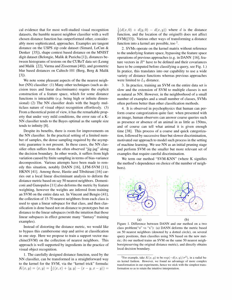
(a) (b)Figure 1. Difference between DANN and our method on a twoclass problem(“o” vs “x”): (a) DANN deforms the metric basedon 50 nearest neighbors (denoted by a dotted circle), on severalquery positions, then classifies using NN based on the new met-ric; (b) our method trains an SVM on the same 50 nearest neigh-bors(preserving the original distance metric), and directly obtainslocal decision boundary.

2For example, take K(x, y) to be exp(−d(x, y)/σ2), in a radial ba-sis kernel fashion. However, we found no advantage of more complextransformation in our experiments, hence we stick with the simplest trans-formation so as to retain the intuitive interpretation.

The philosophy of our work is similar to that of “LocalLearning”, by Bottou and Vapnik [6], in which they pursuedthe same general idea by using K-NN followed by a linearclassifier with ridge regularizer. However, by using only aL2 distance, their work was not driven by the constraint toadapt to a complex distance function.

The rest of the paper is organized as follows: in sec-tion 2, we describe our method in detail and view it fromdifferent perspectives; section 3 introduces a number of ef-fective distance functions, section 4 shows the performanceof our method applied to those distance functions in variousbenchmark data sets; we conclude in section 5.

2. SVM-KNNA naive version of the SVM-KNN is: for a query,1. compute distances of the query to all training exam-

ples and pick the nearest K neighbors;2. if the K neighbors have all the same labels, the query

is labeled and exit; else, compute the pairwise distances be-tween the K neighbors;

3. convert the distance matrix to a kernel matrix andapply multiclass SVM;

4. use the resulting classifier to label the query.To implement multiclass SVM in step 3, three vari-

ants from the statistics and learning literature have beentried([21], [9], [31]) on small number of samples from ourdata sets. They produce roughly the same quality of classi-fiers and the DAGSVM([31]) is chosen for its better speed.

The naive version of SVM-KNN is slow mainly becauseit has to compute the distances of the query to all train-ing examples. Here we again borrow the insight from psy-chophysics that humans can perform fast pruning of visualobject categories. In our setting, this translates into the prac-tice of computing a “crude” distance (e.g. L2 distance) toprune the list of neighbors before the more costly “accu-rate” distance computation. The reason is simply that if thecrude distance is big enough then it is almost certain that theaccurate distance will not be small. This idea works wellin the sense that the performance of the classifier is oftenunaffected whereas the computation is orders-of-magnitudefaster. Earlier instances of this idea in computer vision canbe found in Simard et al. [36] and Mori et al. [25]. We termthis idea “shortlisting”.

An additional trick to speed up the algorithm is to cachethe pairwise distance matrix in step 2. This follows from theobservation that those training examples who participate inthe SVM classification lie closely to the decision boundaryand are likely to be invoked repeatedly during query time.

After the preceding ideas are incorporated, the steps ofthe SVM-KNN are: for a query,

1. Find a collection of Ksl neighbors using a crude dis-tance function (e.g. L2);

2. Compute the “accurate” distance function (e.g. tangentdistance) on the Ksl samples and pick the K nearestneighbors;

3. Compute (or read from cache if possible) the pairwise“accurate” distance of the union of the K neighborsand the query;

4. Convert the pairwise distance matrix into a kernel ma-trix using the “kernel trick”;

5. Apply DAGSVM on the kernel matrix and label thequery using the resulting classifier.

So far there are two perspectives to look at SVM-KNN:it can be viewed as an improvement over NN classifier, orit can be viewed as a model of the discriminative processplausible in biological vision. From a machine learning per-spective, it can also be viewed as an continuum between NNand SVM: when K is small(e.g. K = 5), the algorithm be-haves like a straightforward K-NN classifiers. To the otherextreme, when K = n our method reduces to an overallSVM.

Note, for a large data set, or when the distance functionis costly to evaluate, the training of DAGSVM becomes in-tractable even with state-of-the-art techniques such as se-quential minimal optimization(SMO) (Platt [30]) because itneeds to evaluate O(n2) pairwise “accurate” distances. Incontrast, SVM-KNN is still feasible as long as one can eval-uate the “crude” distance for the nearest neighbor searchand train the local SVM within reasonable time. A compar-ison in time complexity is summarized in Table 1.

DAGSVM SVM-KNNTraining O(Caccun2) noneQuery O(Caccu#SV) O(Ccruden + Caccu(Ksl + K2))

Table 1. Comparison of time complexity, where n is the number oftraining examples, #SV the number of support vectors, Caccu andCcrude the cost for computing accurate and crude distances, Ksl

the length of the shortlist, and K the length of the list participatingin SVM classification.

3. Shape and texture distances

In applying SVM-KNN, we focus our efforts on classi-fying based on the two major cues in visual object recog-nition: shape and texture. We introduce several well-performing distances functions as follows:

3.1. χ2 distance for texture

Following Leung and Malik [22], an image of texture canbe mapped to a histogram of “textons”, which captures the

distribution of different types of texture elements. The dis-tance is defined as the Pearson’s χ2 test statistic [5] betweenthe two texton histograms.

3.2. Marginal distance for texture

From a statistical perspective, the χ2 distance above fortexture can be viewed as measuring the difference betweentwo joint distributions of texture responses: a piece of tex-ture is passed through a bank of filters, the joint distributionof responses are vector-quantized into textons, and the his-togram of textons are compared. Levina et al. [23] foundthat the joint distribution can often be well distinguishedfrom each other by simply looking at the difference in themarginals (namely, the histogram of each filter response).Therefore, another distance function for texture is to sumup the distances between response histograms from each fil-ter. This is used in our experiments for real-world imagesthat may contain too many types of textons to be reliablyquantized.

3.3. Tangent distance

Defined on a pair of gray-scale images of digits, tangentdistance [36] is defined as the smallest distance between twolinear subspaces (in the pixel domain Rn where n is thenumber of pixels), derived from the images by includingperturbations from small affine transformation of the spatialdomain and change in the thickness of pen-stroke (forminga 7-dimensional linear space).

3.4. Shape context based distance

The basic idea of shape context [1] is as follows: Theshape is represented by a point set, with a descriptor at acontrol point to capture the “landscape” around that point.Those descriptors are iteratively matched using a deforma-tion model. And the distance is derived from the discrep-ancy left in the final matched shapes and a score that denoteshow far the deformation is from an affine transformation.

3.5. Geometric blur based distance

A number of shape descriptors can be defined on a grayscale image, for instance the shape context descriptor onthe edge map(e.g. [26]), or the SIFT descriptor([24]), or thegeometric blur descriptor([4]). In our experiments, we fo-cus on the geometric blur descriptor. Usually defined on anedge point, the geometric blur descriptor applies a spatiallyvarying blur on the surrounding patch of edge responses.Points further from the center are blurred more to reflecttheir spatial uncertainty under deformation. After this blur-ring, the descriptors are normalized to have L2 norm 1.They are used in two kinds of distances in section 4.4.

3.6. Kernelizing the distance

Asymmetry: (of shape context based distance and geo-metric blur based distance) We simply define a symmetricdistance: d(x, y) + d(y, x), because in practice the discrep-ancy |d(x, y) − d(y, x)| is small.

Triangle Inequality: (of tangent distance, shape contextbased distance and geometric blur based distance) Namely,the inequality d(x, y) + d(y, z) ≥ d(x, z) does not hold atall times, which prevents the distance from translating intoa positive-definite kernel. A number of solutions have beensuggested for this issue [29]. Here, we compute the small-est eigenvalue of the kernel matrix and if it is negative, weadd its absolute value to the diagonal of the kernel matrix.Intuitively, if we view the kernel matrix as a kind of “sim-ilarity measure”, adding a positive constant to the diagonalmeans strengthening self-similarity, which should not affectthe sense of expressed similarity among the examples.

4. Performance on benchmark data sets4.1. MNIST

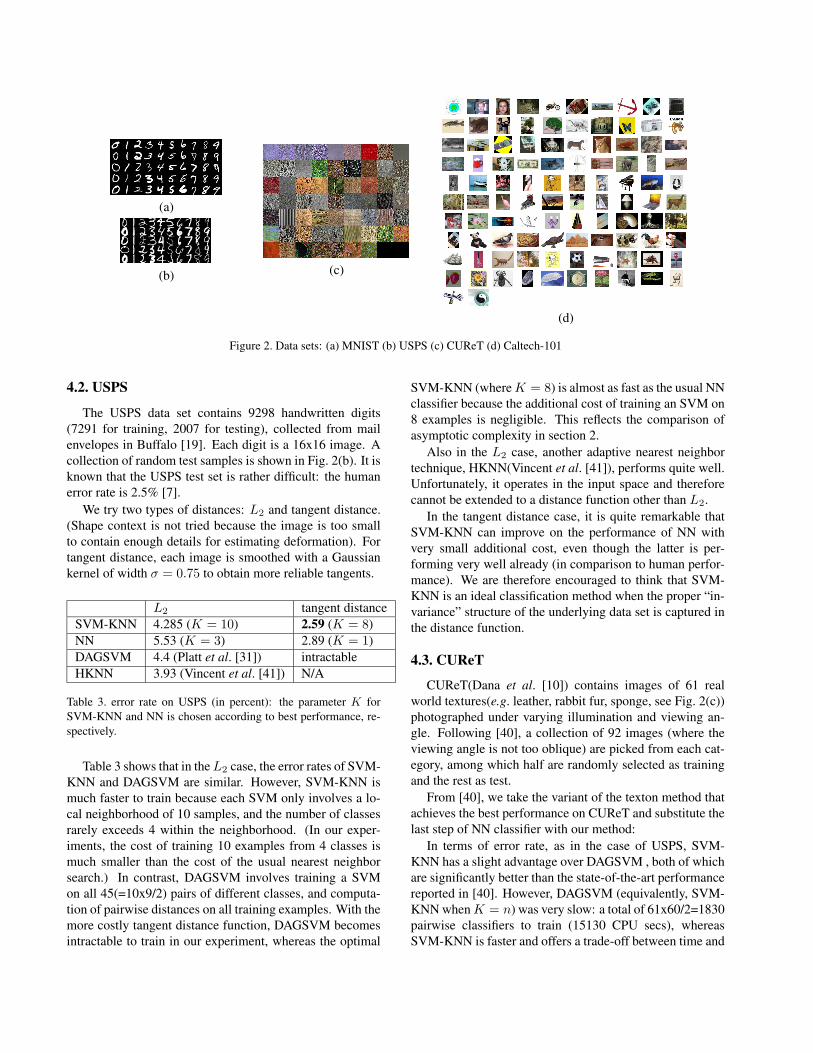
The MNIST data set of handwritten digits contains60,000 examples for training and 10,000 for test: each setcontains equal number of digits from two distinct popu-lations: Census Bureau employees and high school stu-dents [20]. Each digit is a 28x28 image, except for shapecontext computation where each digit is resized to 70x70image. Some example digits from the test set are shown inFig. 2(a). A number of state-of-the-art algorithms performunder 1% error rate, among which a shape context basedmethod performs at .67%.

Two distances are used in this experiment: L2 and shapecontext distance. For shape context, since its error rate maybe close to the Bayes optimal, we use only the first 10,000training examples so as to leave room of improvement (onthe 10,000 examples we perform a 10 fold cross validation).To rely purely on shape context and not on image intensi-ties, we also drop the “appearance” term in [1].

A summary of results is in Table 2. Note that whileL2 distance is straightforward for our method, a numberof workarounds were necessary for the shape context baseddistance. Still, in both cases the performance improves sig-nificantly.

L2 SC (limited training)SVM-KNN 1.66 (K = 80) 1.67 (±0.49) (K = 20)NN 2.87 (K = 3) 2.2 (±0.77) (K = 1)

Table 2. error rate on MNIST (in percent): the parameter K foreach algorithm is selected according to best performance(in rangeof [1,10] for NN and [5, 10, .., 100] for SVM-KNN). In SVM-KNN, the parameter Ksl ≈ 10K, larger Ksl doesn’t improve theempirical results.

(a)

(b) (c)

(d)

Figure 2. Data sets: (a) MNIST (b) USPS (c) CUReT (d) Caltech-101

4.2. USPS

The USPS data set contains 9298 handwritten digits(7291 for training, 2007 for testing), collected from mailenvelopes in Buffalo [19]. Each digit is a 16x16 image. Acollection of random test samples is shown in Fig. 2(b). It isknown that the USPS test set is rather difficult: the humanerror rate is 2.5% [7].

We try two types of distances: L2 and tangent distance.(Shape context is not tried because the image is too smallto contain enough details for estimating deformation). Fortangent distance, each image is smoothed with a Gaussiankernel of width σ = 0.75 to obtain more reliable tangents.

L2 tangent distanceSVM-KNN 4.285 (K = 10) 2.59 (K = 8)NN 5.53 (K = 3) 2.89 (K = 1)DAGSVM 4.4 (Platt et al. [31]) intractableHKNN 3.93 (Vincent et al. [41]) N/A

Table 3. error rate on USPS (in percent): the parameter K forSVM-KNN and NN is chosen according to best performance, re-spectively.

Table 3 shows that in the L2 case, the error rates of SVM-KNN and DAGSVM are similar. However, SVM-KNN ismuch faster to train because each SVM only involves a lo-cal neighborhood of 10 samples, and the number of classesrarely exceeds 4 within the neighborhood. (In our exper-iments, the cost of training 10 examples from 4 classes ismuch smaller than the cost of the usual nearest neighborsearch.) In contrast, DAGSVM involves training a SVMon all 45(=10x9/2) pairs of different classes, and computa-tion of pairwise distances on all training examples. With themore costly tangent distance function, DAGSVM becomesintractable to train in our experiment, whereas the optimal

SVM-KNN (where K = 8) is almost as fast as the usual NNclassifier because the additional cost of training an SVM on8 examples is negligible. This reflects the comparison ofasymptotic complexity in section 2.

Also in the L2 case, another adaptive nearest neighbortechnique, HKNN(Vincent et al. [41]), performs quite well.Unfortunately, it operates in the input space and thereforecannot be extended to a distance function other than L2.

In the tangent distance case, it is quite remarkable thatSVM-KNN can improve on the performance of NN withvery small additional cost, even though the latter is per-forming very well already (in comparison to human perfor-mance). We are therefore encouraged to think that SVM-KNN is an ideal classification method when the proper “in-variance” structure of the underlying data set is captured inthe distance function.

4.3. CUReT

CUReT(Dana et al. [10]) contains images of 61 realworld textures(e.g. leather, rabbit fur, sponge, see Fig. 2(c))photographed under varying illumination and viewing an-gle. Following [40], a collection of 92 images (where theviewing angle is not too oblique) are picked from each cat-egory, among which half are randomly selected as trainingand the rest as test.

From [40], we take the variant of the texton method thatachieves the best performance on CUReT and substitute thelast step of NN classifier with our method:

In terms of error rate, as in the case of USPS, SVM-KNN has a slight advantage over DAGSVM , both of whichare significantly better than the state-of-the-art performancereported in [40]. However, DAGSVM (equivalently, SVM-KNN when K = n) was very slow: a total of 61x60/2=1830pairwise classifiers to train (15130 CPU secs), whereasSVM-KNN is faster and offers a trade-off between time and

χ2

SVM-KNN 1.73 (±0.24) (K = 70)NN 2.53 (±0.28) (K = 3) [40]DAGSVM 1.75 (±0.25)

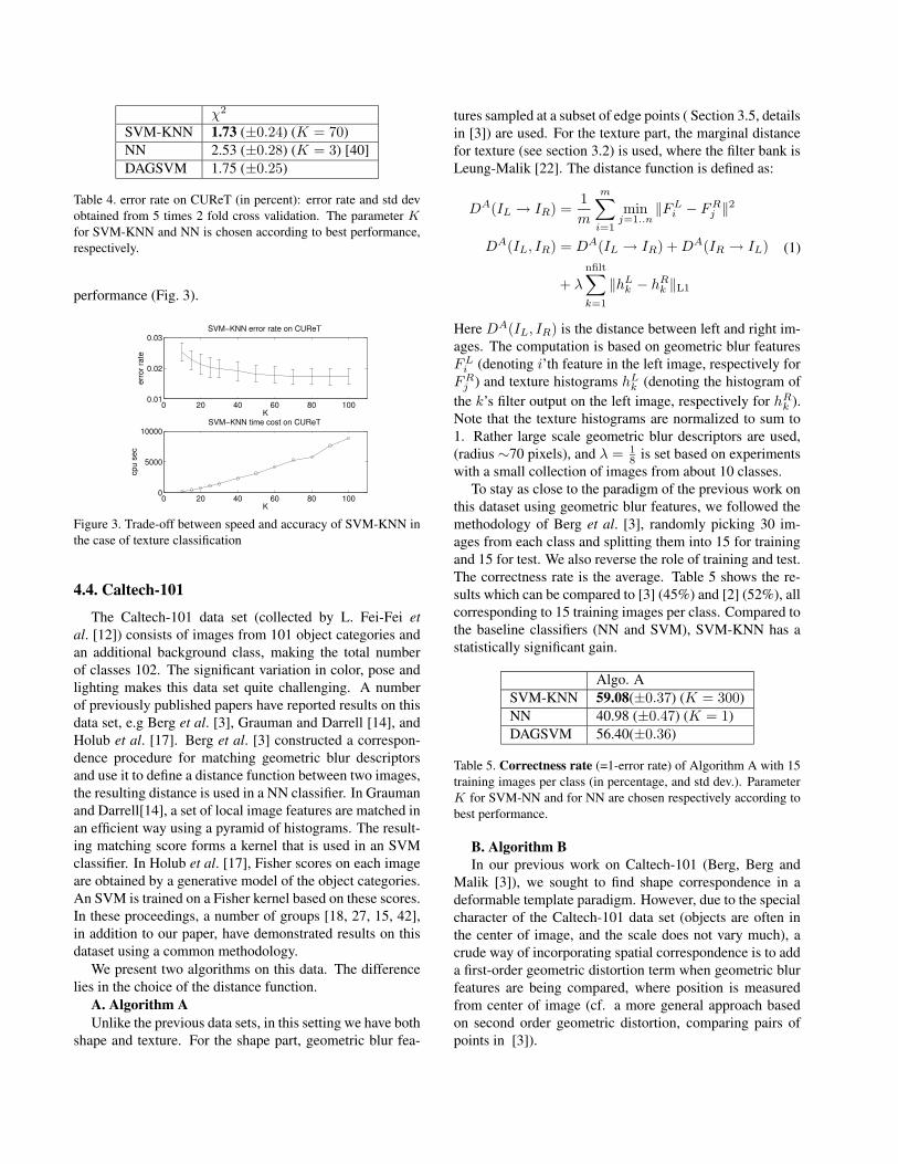
Table 4. error rate on CUReT (in percent): error rate and std devobtained from 5 times 2 fold cross validation. The parameter K

for SVM-KNN and NN is chosen according to best performance,respectively.

performance (Fig. 3).

0 20 40 60 80 1000.01

0.02

0.03SVM−KNN error rate on CUReT

K

erro

r rat

e

0 20 40 60 80 1000

5000

10000SVM−KNN time cost on CUReT

K

cpu

sec

Figure 3. Trade-off between speed and accuracy of SVM-KNN inthe case of texture classification

4.4. Caltech-101

The Caltech-101 data set (collected by L. Fei-Fei etal. [12]) consists of images from 101 object categories andan additional background class, making the total numberof classes 102. The significant variation in color, pose andlighting makes this data set quite challenging. A numberof previously published papers have reported results on thisdata set, e.g Berg et al. [3], Grauman and Darrell [14], andHolub et al. [17]. Berg et al. [3] constructed a correspon-dence procedure for matching geometric blur descriptorsand use it to define a distance function between two images,the resulting distance is used in a NN classifier. In Graumanand Darrell[14], a set of local image features are matched inan efficient way using a pyramid of histograms. The result-ing matching score forms a kernel that is used in an SVMclassifier. In Holub et al. [17], Fisher scores on each imageare obtained by a generative model of the object categories.An SVM is trained on a Fisher kernel based on these scores.In these proceedings, a number of groups [18, 27, 15, 42],in addition to our paper, have demonstrated results on thisdataset using a common methodology.

We present two algorithms on this data. The differencelies in the choice of the distance function.

A. Algorithm AUnlike the previous data sets, in this setting we have both

shape and texture. For the shape part, geometric blur fea-

tures sampled at a subset of edge points ( Section 3.5, detailsin [3]) are used. For the texture part, the marginal distancefor texture (see section 3.2) is used, where the filter bank isLeung-Malik [22]. The distance function is defined as:

DA(IL → IR) =1

m

m∑

i=1

minj=1..n

‖FLi − FR

j ‖2

DA(IL, IR) = DA(IL → IR) + DA(IR → IL)

+ λ

nfilt∑

k=1

‖hLk − hR

k ‖L1

(1)

Here DA(IL, IR) is the distance between left and right im-ages. The computation is based on geometric blur featuresFL

i (denoting i’th feature in the left image, respectively forFR

j ) and texture histograms hLk (denoting the histogram of

the k’s filter output on the left image, respectively for hRk ).

Note that the texture histograms are normalized to sum to1. Rather large scale geometric blur descriptors are used,(radius ∼70 pixels), and λ = 1

8is set based on experiments

with a small collection of images from about 10 classes.To stay as close to the paradigm of the previous work on

this dataset using geometric blur features, we followed themethodology of Berg et al. [3], randomly picking 30 im-ages from each class and splitting them into 15 for trainingand 15 for test. We also reverse the role of training and test.The correctness rate is the average. Table 5 shows the re-sults which can be compared to [3] (45%) and [2] (52%), allcorresponding to 15 training images per class. Compared tothe baseline classifiers (NN and SVM), SVM-KNN has astatistically significant gain.

Algo. ASVM-KNN 59.08(±0.37) (K = 300)NN 40.98 (±0.47) (K = 1)DAGSVM 56.40(±0.36)

Table 5. Correctness rate (=1-error rate) of Algorithm A with 15training images per class (in percentage, and std dev.). ParameterK for SVM-NN and for NN are chosen respectively according tobest performance.

B. Algorithm BIn our previous work on Caltech-101 (Berg, Berg and

Malik [3]), we sought to find shape correspondence in adeformable template paradigm. However, due to the specialcharacter of the Caltech-101 data set (objects are often inthe center of image, and the scale does not vary much), acrude way of incorporating spatial correspondence is to adda first-order geometric distortion term when geometric blurfeatures are being compared, where position is measuredfrom center of image (cf. a more general approach basedon second order geometric distortion, comparing pairs ofpoints in [3]).

In this case, the overall distance function is

DB(IL → IR) =1

m

m∑

i=1

minj=1..n

[

‖FLi − FR

j ‖2 +λ

r0

‖rLi − rR

j ‖

]

DB(IL, IR) = DB(IL → IR) + DB(IR → IL)

(2)

and rLi denotes the pixel coordinates of the i’th geometric

blur feature on the left image, w.r.t. the image center (re-spectively for rR

j ). r0 = 270 is the average image size. Weused a medium scale of geometric blur(radius ∼42 pixels),and λ = 1

4.

Algorithm B is tested with the benchmark methodologyof Grauman and Darrell [15], where a number (say 15) ofimages are taken from each class uniformly at random as thetraining image, and the rest of the data set is used as test set.The “mean recognition rate per class” is used so that morepopulous (and easier) classes are not favored. This processis repeated 10 times and the average correctness rate is re-ported. Our experiments use the DAGSVM classifier. (Wehave yet to run SVM-KNN in this setting but the perfor-mance of SVM-KNN can only be better because it includesDAGSVM as a special case for K = n. ). 3

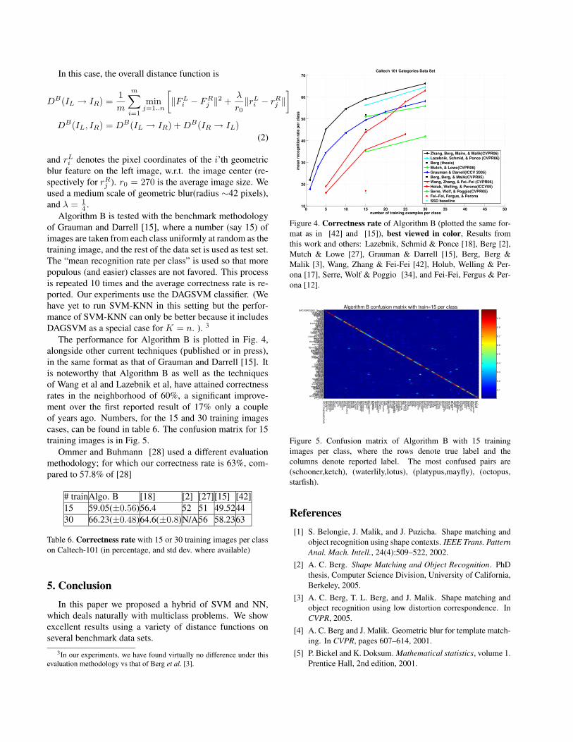
The performance for Algorithm B is plotted in Fig. 4,alongside other current techniques (published or in press),in the same format as that of Grauman and Darrell [15]. Itis noteworthy that Algorithm B as well as the techniquesof Wang et al and Lazebnik et al, have attained correctnessrates in the neighborhood of 60%, a significant improve-ment over the first reported result of 17% only a coupleof years ago. Numbers, for the 15 and 30 training imagescases, can be found in table 6. The confusion matrix for 15training images is in Fig. 5.

Ommer and Buhmann [28] used a different evaluationmethodology; for which our correctness rate is 63%, com-pared to 57.8% of [28]

# trainAlgo. B [18] [2] [27][15] [42]15 59.05(±0.56)56.4 52 51 49.524430 66.23(±0.48)64.6(±0.8)N/A56 58.2363

Table 6. Correctness rate with 15 or 30 training images per classon Caltech-101 (in percentage, and std dev. where available)

5. ConclusionIn this paper we proposed a hybrid of SVM and NN,

which deals naturally with multiclass problems. We showexcellent results using a variety of distance functions onseveral benchmark data sets.

3In our experiments, we have found virtually no difference under thisevaluation methodology vs that of Berg et al. [3].

0 5 10 15 20 25 30 35 40 45 5010

20

30

40

50

60

70

number of training examples per class

mea

n re

cogn

ition

rat

e pe

r cl

ass

Caltech 101 Categories Data Set

Zhang, Berg, Maire, & Malik(CVPR06)Lazebnik, Schmid, & Ponce (CVPR06)Berg (thesis)Mutch, & Lowe(CVPR06)Grauman & Darrell(ICCV 2005)Berg, Berg, & Malik(CVPR05)Wang, Zhang, & Fei−Fei (CVPR06)Holub, Welling, & Perona(ICCV05)Serre, Wolf, & Poggio(CVPR05)Fei−Fei, Fergus, & PeronaSSD baseline

Figure 4. Correctness rate of Algorithm B (plotted the same for-mat as in [42] and [15]), best viewed in color, Results fromthis work and others: Lazebnik, Schmid & Ponce [18], Berg [2],Mutch & Lowe [27], Grauman & Darrell [15], Berg, Berg &Malik [3], Wang, Zhang & Fei-Fei [42], Holub, Welling & Per-ona [17], Serre, Wolf & Poggio [34], and Fei-Fei, Fergus & Per-ona [12].

Algorithm B confusion matrix with train=15 per class

BA

CK

GR

OU

ND

Goo

gle

Face

sFa

ces eas

yLe

opar

dsM

otor

bike

sac

cord

ion

airp

lane

san

chor an

tba

rrel

bass

beav

erbi

nocu

lar

bons

aibr

ain

bron

tosa

urus

budd

habu

tterfl

yca

mer

aca

nnon

car sid

ece

iling

fance

llpho

nech

air

chan

delie

rco

ugar

body

coug

arfac

ecr

abcr

ayfis

hcr

ocod

ilecr

ocod

ilehea

dcu

pda

lmat

ian

dolla

r billdo

lphi

ndr

agon

flyel

ectri

c guita

rel

epha

ntem

ueu

phon

ium

ewer

ferr

yfla

min

gofla

min

gohea

dga

rfiel

dge

renu

kgr

amop

hone

gran

d piano

haw

ksbi

llhe

adph

one

hedg

ehog

helic

opte

rib

isin

line ska

tejo

shua

tree

kang

aroo

ketc

hla

mp

lapt

oplla

ma

lobs

ter

lotu

sm

ando

linm

ayfly

men

orah

met

rono

me

min

aret

naut

ilus

octo

pus

okap

ipa

goda

pand

api

geon

pizz

apl

atyp

uspy

ram

idre

volv

errh

ino

roos

ter

saxo

phon

esc

hoon

ersc

isso

rssc

orpi

onse

a horse

snoo

pyso

ccer

ball

stap

ler

star

fish

steg

osau

rus

stop

sign

stra

wbe

rry

sunf

low

ertic

ktri

lobi

teum

brel

law

atch

wat

erlill

yw

heel

chai

rw

ildcat

win

dsor

chair

wre

nch

yin yan

g

BACKGROUND_GoogleFacesFaces_easyLeopardsMotorbikesaccordionairplanesanchorantbarrelbassbeaverbinocularbonsaibrainbrontosaurusbuddhabutterflycameracannoncar_sideceiling_fancellphonechairchandeliercougar_bodycougar_facecrabcrayfishcrocodilecrocodile_headcupdalmatiandollar_billdolphindragonflyelectric_guitarelephantemueuphoniumewerferryflamingoflamingo_headgarfieldgerenukgramophonegrand_pianohawksbillheadphonehedgehoghelicopteribisinline_skatejoshua_treekangarooketchlamplaptopllamalobsterlotusmandolinmayflymenorahmetronomeminaretnautilusoctopusokapipagodapandapigeonpizzaplatypuspyramidrevolverrhinoroostersaxophoneschoonerscissorsscorpionsea_horsesnoopysoccer_ballstaplerstarfishstegosaurusstop_signstrawberrysunflowerticktrilobiteumbrellawatchwater_lillywheelchairwild_catwindsor_chairwrenchyin_yang

0.1

0.2

0.3

0.4

0.5

0.6

0.7

0.8

0.9

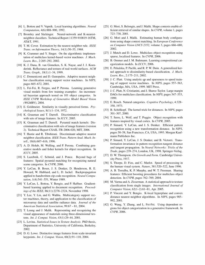
Figure 5. Confusion matrix of Algorithm B with 15 trainingimages per class, where the rows denote true label and thecolumns denote reported label. The most confused pairs are(schooner,ketch), (waterlily,lotus), (platypus,mayfly), (octopus,starfish).

References[1] S. Belongie, J. Malik, and J. Puzicha. Shape matching and

object recognition using shape contexts. IEEE Trans. PatternAnal. Mach. Intell., 24(4):509–522, 2002.

[2] A. C. Berg. Shape Matching and Object Recognition. PhDthesis, Computer Science Division, University of California,Berkeley, 2005.

[3] A. C. Berg, T. L. Berg, and J. Malik. Shape matching andobject recognition using low distortion correspondence. InCVPR, 2005.

[4] A. C. Berg and J. Malik. Geometric blur for template match-ing. In CVPR, pages 607–614, 2001.

[5] P. Bickel and K. Doksum. Mathematical statistics, volume 1.Prentice Hall, 2nd edition, 2001.

[6] L. Bottou and V. Vapnik. Local learning algorithms. NeuralComputation, 4(6):888–900, 1992.

[7] Bromley and Sackinger. Neural-network and K-nearest-neighbor classifiers. Technical Report 11359-910819-16TM,AT&T, 1991.

[8] T. M. Cover. Estimation by the nearest neighbor rule. IEEETrans. on Information Theory, 14(1):50–55, 1968.

[9] K. Crammer and Y. Singer. On the algorithmic implemen-tation of multiclass kernel-based vector machines. J. Mach.Learn. Res., 2:265–292, 2002.

[10] K. J. Dana, B. van Ginneken, S. K. Nayar, and J. J. Koen-derink. Reflectance and texture of real-world surfaces. ACMTrans. Graph., 18(1):1–34, 1999.

[11] C. Domeniconi and D. Gunopulos. Adaptive nearest neigh-bor classification using support vector machines. In NIPS,pages 665–672, 2001.

[12] L. Fei-Fei, R. Fergus, and P. Perona. Learning generativevisual models from few training examples: An incremen-tal bayesian approach tested on 101 object categories. InIEEE CVPR Workshop of Generative Model Based Vision(WGMBV), 2004.

[13] E. Goldmeier. Similarity in visually perceived forms. Psy-chological Issues, 8(1):1–134, 1972.

[14] K. Grauman and T. Darrell. Discriminative classificationwith sets of image features. In ICCV, 2005.

[15] K. Grauman and T. Darrell. Pyramid match kernels: Dis-criminative classification with sets of image features (version2). Technical Report CSAIL-TR-2006-020, MIT, 2006.

[16] T. Hastie and R. Tibshirani. Discriminant adaptive nearestneighbor classification. IEEE Trans. Pattern Anal. Mach. In-tell., 18(6):607–616, 1996.

[17] A. D. Holub, M. Welling, and P. Perona. Combining gen-erative models and fisher kernels for object recognition. InICCV, 2005.

[18] S. Lazebnik, C. Schmid, and J. Ponce. Beyond bags offeatures: Spatial pyramid matching for recognizing naturalscene categories. In CVPR, 2006.

[19] Y. LeCun, B. Boser, J. S. Denker, D. Henderson, R. E.Howard, W. Hubbard, and L. D. Jackel. Backpropagationapplied to handwritten zip code recognition. Neural Compu-tation, 1(4):541–551, Winter 1989.

[20] Y. LeCun, L. Bottou, Y. Bengio, and P. Haffner. Gradient-based learning applied to document recognition. Proceed-ings of the IEEE, 86(11):2278–2324, November 1998.

[21] Y. Lee, Y. Lin, and G. Wahba. Multicategory support vec-tor machines, theory, and application to the classification ofmicroarray data and satellite radiance data. Journal of theAmerican Statistical Association, 99:67 – 81, 2004.

[22] T. Leung and J. Malik. Representing and recognizing thevisual appearance of materials using three-dimensional tex-tons. Int. J. Comput. Vision, 43(1):29–44, 2001.

[23] L. Levina. Statistical Issues in Texture Analysis. PhD thesis,Department of Statistics, University of California, Berkeley,2002.

[24] D. G. Lowe. Distinctive image features from scale-invariantkeypoints. Int. J. Comput. Vision, 60(2):91–110, 2004.

[25] G. Mori, S. Belongie, and J. Malik. Shape contexts enable ef-ficient retrieval of similar shapes. In CVPR, volume 1, pages723–730, 2001.

[26] G. Mori and J. Malik. Estimating human body configura-tions using shape context matching. In European Conferenceon Computer Vision LNCS 2352, volume 3, pages 666–680,2002.

[27] J. Mutch and D. Lowe. Multiclass object recognition usingsparse, localized features. In CVPR, 2006.

[28] B. Ommer and J. M. Buhmann. Learning compositional cat-egorization models. In ECCV, 2006.

[29] E. Pekalska, P. Paclik, and R. P. W. Duin. A generalized ker-nel approach to dissimilarity-based classification. J. Mach.Learn. Res., 2:175–211, 2002.

[30] J. C. Platt. Using analytic qp and sparseness to speed train-ing of support vector machines. In NIPS, pages 557–563,Cambridge, MA, USA, 1999. MIT Press.

[31] J. C. Platt, N. Cristianini, and J. Shawe-Taylor. Large marginDAGs for multiclass classification. In NIPS, pages 547–553,1999.

[32] E. Rosch. Natural categories. Cognitive Psychology, 4:328–350, 1973.

[33] B. Scholkopf. The kernel trick for distances. In NIPS, pages301–307, 2000.

[34] T. Serre, L. Wolf, and T. Poggio. Object recognition withfeatures inspired by visual cortex. In CVPR, 2005.

[35] P. Simard, Y. LeCun, and J. S. Denker. Efficient patternrecognition using a new transformation distance. In NIPS,pages 50–58, San Francisco, CA, USA, 1993. Morgan Kauf-mann Publishers Inc.

[36] P. Simard, Y. LeCun, J. S. Denker, and B. Victorri. Trans-formation invariance in pattern recognition-tangent distanceand tangent propagation. In Neural Networks: Tricks of theTrade, pages 239–274, London, UK, 1998. Springer-Verlag.

[37] D. W. Thompson. On Growth and Form. Cambridge Univer-sity Press, 1917.

[38] S. Thorpe, D. Fize, and C. Marlot. Speed of processing inthe human visual system. Nature, 381:520–522, June 1996.

[39] A. B. Torralba, K. P. Murphy, and W. T. Freeman. Sharingfeatures: Efficient boosting procedures for multiclass objectdetection. In CVPR, pages 762–769, 2004.

[40] M. Varma and A. Zisserman. A statistical approach to textureclassification from single images. International Journal ofComputer Vision, 62(1–2):61–81, Apr. 2005.

[41] P. Vincent and Y. Bengio. K-local hyperplane and convexdistance nearest neighbor algorithms. In NIPS, pages 985–992, 2001.

[42] G. Wang, Y. Zhang, and L. Fei-Fei. Using dependent re-gions for object categorization in a generative framework. InCVPR, 2006.