sven reiche ucla icfa-workshop - sardinia 07/02

Sven Reiche - ICFA Sardinia

Comparison of the Coherent Radiation-induced

Microbunch Instability in an FEL and a Magnetic Chicane

Comparison of the Coherent Radiation-induced

Microbunch Instability in an FEL and a Magnetic Chicane

Sven Reiche

UCLA

ICFA-Workshop - Sardinia 07/02


The AnalogyThe Analogy

Gun UndulatorChicaneLinac

A Typical FEL Beamline

Linac

Trajectory

Instability I I

CSR SASE FEL


The Resonance ApproximationThe Resonance Approximation

The FEL model is based on the resonance approximation

€

<βz >=k

k + ku

The consequences of this assumption are:• Energy change per period is small• Electron motion can be averaged over the undulator period• Selection of a small bandwidth around central, resonant

frequency• Radiation field is interacting with electron beam over entire

undulator length, although the changes per period are small as well


The FEL Model (1D)The FEL Model (1D)

FEL equations

€

dθ j

dζ= Δ + δ j

dδ j

dζ= −[(A + iσ e−iθ j )e iθ j + c.c.]

dA

dζ= e−iθ j

Pondemotive phase=(k+ku)z-t

Deviation of mean energy 0 from resonant energy R Deviation of particle

energy from mean energy

Space charge parameter

Radiation field ampitude

Normalized position in undulator =2kus

Universal scaling parameter

€

=Kfcγ oωp

4cγ R2 ku

⎡

⎣ ⎢

⎤

⎦ ⎥

2

3

Linear in energy deviation

Linear in field amplitude

Linear in bunching


Solutions of the FEL EquationsSolutions of the FEL Equations

The ansatz A~exp[i] yields a dispersion function for with the initial energy distribution f() as argument.

€

1

Λ−σ

⎛

⎝ ⎜

⎞

⎠ ⎟

∂f

∂δ∫ 1

Λ + Δ + δdδ = −1

In the simplest case (3=-1) there are three roots, corresponding to• an exponentially growing mode,• an exponentially decaying mode,• an oscillating mode.The model is only valid as long the resonance approximation is fulfilled.

€

<<1


The Limit of the FEL ModelThe Limit of the FEL Model

What happened for ~ 1 ?Technically the FEL model is based on perturbation theory in first order with as the order parameter. Approaching unity requires higher order and gives poor convergence!

Qualitatively the limit corresponds to a significant growth within one period. The explicit motion of the electrons has to be taken into account. Currently no such device exist!

A chicane is different because the transverse offset is larger than the beam size. Radiation interacts for short time before leaving the bunch. This allows to model the radiation by an instantaneously acting wake potential.


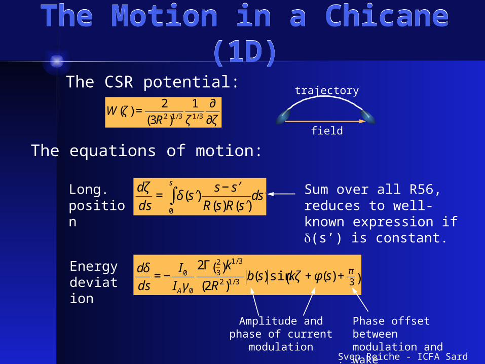
The Motion in a Chicane (1D)The Motion in a Chicane (1D)

The CSR potential:

€

W (ζ ) =2

(3R2)1/ 3

1

ζ 1/ 3

∂

∂ζfield

trajectory

€

dδ

ds= −

I0

IAγ 0

2Γ 2

3( )k1/ 3

(2R2)1/ 3b(s) sin kζ + φ(s) + π

3( )€

dζ

ds= δ( ′ s )

s − ′ s

R(s)R( ′ s )0

s

∫ d ′ s

The equations of motion:

Long. position

Energy deviation

Sum over all R56, reduces to well-known expression if (s’) is constant.

Amplitude and phase of current modulation

Phase offset between modulation and wake


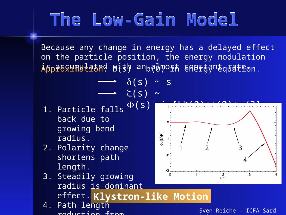
The Low-Gain ModelThe Low-Gain ModelBecause any change in energy has a delayed effect on the particle position, the energy modulation is accumulated with an almost constant rate.Approximation: b(s) ~ b(0) in energy equation.

1. Particle falls back due to growing bend radius.

2. Polarity change shortens path length.

3. Steadily growing radius is dominant effect.

4. Path length reduction from bend 1 & 2 are combined.

1 2 3

4

(s) ~ s(s) ~ (s).sin[k(0)+(0)+/3]

Klystron-like Motion


The Gain in the Low-Gain ModelThe Gain in the Low-Gain Model

The final gain, including energy spread is

€

ξ =I0Γ

2

3( )

2IAγ 0

8L3k

3R2

⎛

⎝ ⎜

⎞

⎠ ⎟

4

3

Example:Generic LCLS chicane = 500, I0 = 100 A, R = 12 m, L = 1.5 m)

€

G = e−α ξ3

2 1+ ξ + ξ 2

€

α =IAγ 0

2I0Γ 2 /3( )

⎛

⎝ ⎜

⎞

⎠ ⎟

3

σ δ2with and

α=0 α=0.003

α=0.015

α=0.05

€

ξ =25 ⇔ λ = 5μm


LimitationsLimitationsThe model is limited by

1. Negligible growth of the modulation in the first half of chicane.

2. Negligible change in the bunching phase.

Low-gain model

Heifets et al. model

High-gain regime of microbunch instability

Comparison of low gain model with self-consistent model byHeifets, Krinsky andStupakov


High-Gain ModelHigh-Gain Model

Check for high-gain growth in a single dipole.

Collective variables:

€

B = −ik e−iΨζ

€

Δ = e−iΨδ

Current modulation Energy modulation

Differential equations:

€

dΔ

ds= −

ρ csr4

kR2e i π

3 B

dB

ds= −i

k

R2Δ(s − s')ds'

0

s

∫

with

€

csr =I0

IAγ 0

413 Γ 2

3( ) ⎡

⎣ ⎢

⎤

⎦ ⎥

14

kR( )13

3rd order in energy modulation

Linear in bunching


Solution Solution

Dispersion equation for the ansatz B~exp[is] :

€

4 =ρ csr

R

⎛

⎝ ⎜

⎞

⎠ ⎟4

e i 5π6

Dispersion equation has 4 roots corresponding to• 2 exponentially growing modes,• 2 exponentially decaying modes.

The maximum growth rate is |Im(1)|=(csr/R)sin(7/24) and the characteristic length (gain length) of the instability is R/csr (for the FEL the characteristic length is 4U/).


When Does ‘High-Gain’ Apply? When Does ‘High-Gain’ Apply?

The exponentional growth is limited by two effects:

1. Finite length of the dipole

2. Start-up lethargy€

csr >R

L>>1

Needs at least 4 gain lengths to show significant growth in modulation.


Energy SpreadEnergy Spread

With given expression for equations of motion, energy spread is difficult to incorporate (e.g.Vaslov equation).

Qualitative Analysis:

Energy spread is converted into phase spread as

€

σΨ =k

6R2s3σ δ =

IAγ 0

I0Γ23( )

⎡

⎣ ⎢

⎤

⎦ ⎥

3

4 σ δ

72

sρ csr

R

⎛

⎝ ⎜

⎞

⎠ ⎟3

≡ ˆ σ δ ˆ s 3

Phase spread is independent on modulation wavelength or bend radius in measures of the gain length.

Estimate for high-gain threshold:

€

ˆ σ δ < 0.02


Final ComparisonFinal Comparison

FEL Magnet Chicane

Modes (1D) 3 4

Scaling Parameter ( << 1

>> 1

(low gain > 1)

Frequency Band Narrow Wide

ApproximationResonance

ApproximationWake Potential

Electron Motion Averaged Explicit

Radiation FieldContinuous

OverlapShort Overlap


ConclusionConclusionInstabilities have same principle of interaction between electron beam and synchrotron radiation, but the signature is different for the different characteristic sizes of the devices.

Characteristic Parameter

Chicane FELUnknown

>> 1 ~ 1 << 1

Presented model valid for special chicane layout (no drifts), but many results can qualitatively be applied to other cases.

sven reiche ucla icfa-workshop - sardinia 07/02

Documents