In cooperation with Tufts University

Surface Wave Site Characterization at 27 Locations Near Boston, Massachusetts, Including 2 Strong-Motion Stations

Open-File Report 2014–1232

U.S. Department of the Interior U.S. Geological Survey

U.S. Department of the Interior SALLY JEWELL, Secretary

U.S. Geological Survey Suzette M. Kimball, Acting Director

U.S. Geological Survey, Reston, Virginia: 2014

For more information on the USGS—the Federal source for science about the Earth, its natural and living resources, natural hazards, and the environment—visit http://www.usgs.gov or call 1–888–ASK–USGS (1–888–275–8747)

For an overview of USGS information products, including maps, imagery, and publications, visit http://www.usgs.gov/pubprod

To order this and other USGS information products, visit http://store.usgs.gov

Any use of trade, firm, or product names is for descriptive purposes only and does not imply endorsement by the U.S. Government.

Although this information product, for the most part, is in the public domain, it also may contain copyrighted materials as noted in the text. Permission to reproduce copyrighted items must be secured from the copyright owner.

Suggested citation: Thompson, E.M., Carkin, B., Baise, L.G., and Kayen, R.E., 2014, Surface wave site characterization at 27 locations near Boston, Massachusetts, including 2 strong-motion stations: U.S. Geological Survey Open-File Report 2014–1232, 27 p., http://dx.doi.org/10.3133/ofr20141232.

ISSN 2331-1258 (online)

iii

Contents Introduction .................................................................................................................................................................... 1 Study Area and Geology ................................................................................................................................................ 2 Field Methods ................................................................................................................................................................ 4 Data Processing ............................................................................................................................................................ 4 Forward Modeling .......................................................................................................................................................... 5 Results ........................................................................................................................................................................... 5 Resources ...................................................................................................................................................................... 7 Acknowledgments .......................................................................................................................................................... 7 References Cited ........................................................................................................................................................... 8 Appendix 1. Shear-Wave Velocity Profiles .................................................................................................................. 10 Appendix 2. Site Descriptions ..................................................................................................................................... 19

Figures 1. Map of the Boston, Massachusetts, area showing spectral analysis of surface waves sites. .................................... 2 2. Surface-wave shaker-trailer (USGS Velociraptor) testing at Millenium Park in West Roxbury, Mass. ....................... 3 3. Velocity profiles along two transects: A, the Charles River, and B, the Mystic River. ................................................ 7

Tables 1. Spectral analysis of surface waves (SASW) summary information. ........................................................................... 6

Surface Wave Site Characterization at 27 Locations Near Boston, Massachusetts, Including 2 Strong-Motion Stations

By Eric M. Thompson1, Brad Carkin2, Laurie G. Baise1, and Robert E. Kayen2

Introduction The geotechnical properties of the soils in and around Boston, Massachusetts, have been

extensively studied. This is partly due to the importance of the Boston Blue Clay and the extent of landfill in the Boston area. Although New England is not a region that is typically associated with seismic hazards, there have been several historical earthquakes that have caused significant ground shaking (for example, see Street and Lacroix, 1979; Ebel, 1996; Ebel, 2006). The possibility of strong ground shaking, along with heightened vulnerability from unreinforced masonry buildings, motivates further investigation of seismic hazards throughout New England. Important studies that are pertinent to seismic hazards in New England include source-parameter studies (Somerville and others, 1987; Boore and others, 2010), wave-propagation studies (Frankel, 1991; Viegas and others, 2010), empirical ground-motion prediction equations (GMPE) for computing ground-motion intensity (Tavakoli and Pezeshk, 2005; Atkinson and Boore, 2006), site-response studies (Hayles and others, 2001; Ebel and Kim, 2006), and liquefaction studies (Brankman and Baise, 2008). The shear-wave velocity (VS) profiles collected for this report are pertinent to the GMPE, site response, and liquefaction aspects of seismic hazards in the greater Boston area. Besides the application of these data for the Boston region, the data may be applicable throughout New England, through correlations with geologic units (similar to Ebel and Kim, 2006) or correlations with topographic slope (Wald and Allen, 2007), because few VS measurements are available in stable tectonic regions.

Ebel and Hart (2001) used felt earthquake reports to infer amplification patterns throughout the greater Boston region and noted spatial correspondence with the dominant period and amplification factors obtained from ambient noise (horizontal-to-vertical ratios) by Kummer (1998). Britton (2003) compiled geotechnical borings in the area and produced a microzonation map based on generalized velocity profiles, where the amplifications were computed using Shake (Schnable and others, 1972), along with an assumed input ground motion. The velocities were constrained by only a few local measurements associated with the Central Artery/Tunnel project. The additional VS measurements presented in this report provide a number of benefits. First, these measurements provide improved spatial coverage. Second, the larger sample size provides better constraints on the mean and variance of the VS distribution for each layer, which may be paired with a three-dimensional (3D) model of the stratigraphy to generate one-dimensional (1D) profiles for use in a standard site-response analysis (for example, Britton, 2003). Third, the velocity profiles may also be used, along with a 3D model of the

1Tufts University. 2U.S. Geological Survey.

2

stratigraphy, as input into a 3D simulation of the ground motion to investigate the effects of basin-generated surface waves and the potential focusing of seismic waves.

This report begins with a short review of the geology of the study area and the field methods that we used to estimate the velocity profiles. The raw data, processed data, and the interpreted VS profiles are given in appendix 1. Photographs and descriptions of the sites are provided in appendix 2. The VS layered models can also be downloaded from the Web site associated with this report.

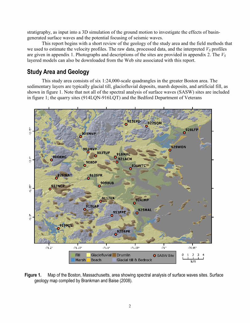
Study Area and Geology This study area consists of six 1:24,000-scale quadrangles in the greater Boston area. The

sedimentary layers are typically glacial till, glaciofluvial deposits, marsh deposits, and artificial fill, as shown in figure 1. Note that not all of the spectral analysis of surface waves (SASW) sites are included in figure 1; the quarry sites (914LQN-916LQT) and the Bedford Department of Veterans

Figure 1. Map of the Boston, Massachusetts, area showing spectral analysis of surface waves sites. Surface geology map compiled by Brankman and Baise (2008).

3

Affairs (VA) Hospital site (907BVA) were selected for reasons other than characterizing the Boston region, and they are located significantly outside of the mapped area. The population in this region is widely distributed over a larger area, and it would be valuable for future work to extend the study area to a larger geographic extent.

The sediments in the Boston area were primarily deposited during and after the extensive Pleistocene glaciations (Kaye, 1982; Barosh and others, 1989; Woodhouse and others, 1991). The glacial till generally overlies bedrock and consists of very dense, poorly sorted sand, gravel, and cobbles in a clay matrix. The glaciofluvial deposits include outwash, eskers, kettles, kame fields, and terrace deposits that formed through the transport of glacially derived materials. These deposits are typically densely consolidated, stratified sands and gravels. Other sediments in this region include the Boston Blue Clay, marsh, beach sand, and fill. The fill often overlies marsh deposits. The Boston Blue Clay is extensively studied in the geotechnical engineering community and consists of clay, silt, and fine sand. Much of the Boston Blue Clay has been loaded during glacial advances, and thus the shallower deposits often show a large overconsolidation ratio, which could result in a VS profile where the velocity decreases with depth, sometimes referred to as a velocity inversion. The shallow bedrock in this area is typically the Cambridge Argillite, which includes layers of tuff and sandstone, as well as intrusive sills and dikes of diabase, diorite, and basalt (Johnson, 1989).

Johnson (1989) synthesizes the geology of the Boston area into three typical profiles. As noted above, the till layer (1.5–9 m) generally overlies bedrock, which is typically encountered within 100 m of the surface. The glacial till is generally overlain by a thick layer of the Boston Blue Clay (12–43 m), which is often stiffer at shallower depths. A thin layer of glaciofluvial deposits (0–7.5 m) often overlies the clay, followed by 1.5–9 m of organic material, and 3–9 m of fill. See Johnson (1989) for more details, including other variations on the typical Boston profile.

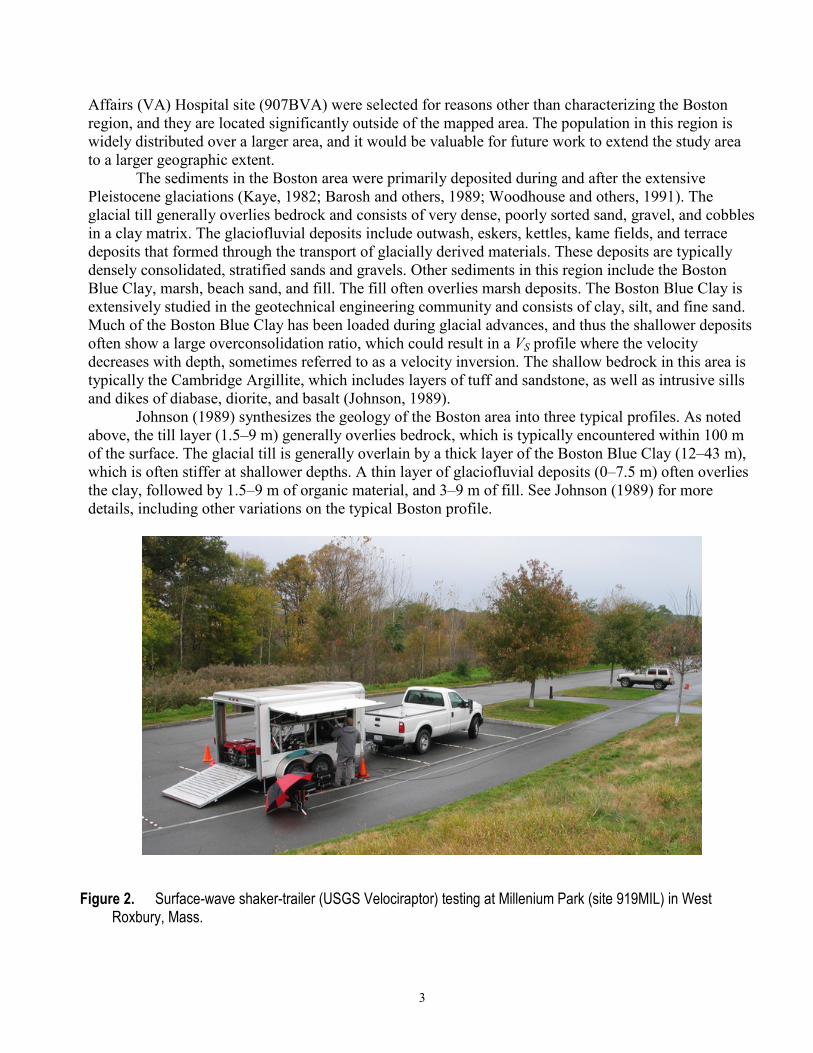
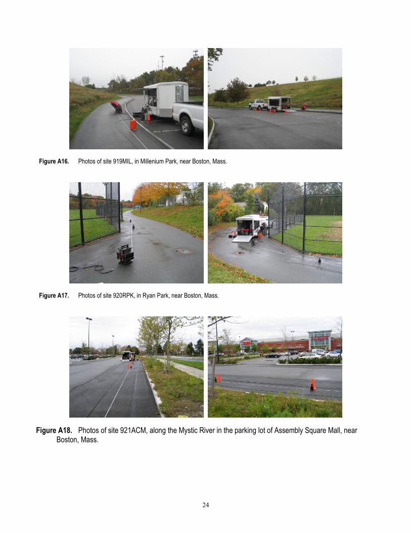
Figure 2. Surface-wave shaker-trailer (USGS Velociraptor) testing at Millenium Park (site 919MIL) in West Roxbury, Mass.

4

Field Methods For this project, we use the noninvasive and nondestructive SASW method. The general

approach is to measure the phase velocity of Rayleigh surface waves, which can then be used to infer the VS profile. There are many variations on this general method, which vary in terms of the source of the Rayleigh waves, the equipment used to measure their phase velocities, and the number of modes that are included in the analysis. The SASW method we employ focuses on the fundamental mode of Rayleigh waves that are actively controlled by vertically loading the ground surface with a parallel array of mass shakers. The shakers that we use have a long stroke capable of cycling as low as 1 Hz, well below the normal 7-Hz cut-off frequency of a vibroseis truck. The output signal from the spectral analyzer is split into a parallel circuit and sent to separate amplifiers. The amplifiers power the shakers to produce a coherent phase continuous harmonic-wave that vertically loads the ground. Most of this energy produces Rayleigh surface waves. We sweep across frequencies from 1 to 200 Hz.

Data Processing Frequency domain analyses are made on two or more signals received by sensors placed in the

field in the linear array some distance from the source. First, all channels of time-domain data are transformed into their equivalent linear spectrum in the frequency domain by using a Fourier transform. One of the sensor’s signals (typically the sensor closest to the source) is used for a reference input signal, and the other sensor signals are used to compute the linear spectrums of the output. The separation of the reference seismometer and output seismometer (ds – dref) radially from the source is used later to compute the velocity. The cross-power spectrum is defined as

𝐺𝑥𝑥(𝜔) = 𝑆𝑥∗(𝜔)𝑆𝑥(𝜔) , (1)

where 𝑆𝑥∗ is the complex conjugate of the linear spectrum of the input signal and 𝑆𝑥 is the real part of the linear spectrum of the output signal. The cross-power spectrum can be represented by its real and imaginary components, or by its phase 𝜃, and amplitude A. The phase can be stacked to enhance signal-to-noise ratio because it is a relative quantity. The phase of 𝐺𝑥𝑥 is computed as the inverse tangent of the ratio of the imaginary and real portions of the cross-power spectrum:

𝜃𝑥𝑥(𝜔) = atan 𝐼𝐼(𝐺𝑥𝑥(𝜔))𝑅𝑅(𝐺𝑥𝑥(𝜔)) ,

(2)

where Im() is the imaginary part of the cross power spectrum, and Re() is the real part of the cross- power spectrum. The travel time of one cycle of a wave is

𝑡(𝑓) = 𝜃(𝜔)/𝜔 , (3)

where f is the frequency. The wavelength is

𝜆(𝜃) = (𝑑𝑠 − 𝑑ref)/𝜃(𝑓) . (4)

5

The Rayleigh wave velocity is

𝑉𝑟(𝑓) = 𝑑𝑠−𝑑ref𝑡(𝑓) = 𝑓𝜆(𝜃) .

(5)

The evaluation of velocities is constrained to the wavelength zone where 𝜆(𝜃)/3 < (𝑑𝑠 −

𝑑ref) < 2𝜆(𝜃) for typical data and 𝜆(𝜃)/3 < (𝑑𝑠 − 𝑑ref) < 3𝜆(𝜃) for excellent data, corresponding to phase lags of 180–1,080° (typical data) and 120–1,080° (excellent data). At longer and shorter wavelengths the data become unreliable for computing velocities.

Forward Modeling As mentioned previously, the soft sediments in this region often overlie hard bedrock.

Additionally, the Boston Blue Clay may show a velocity inversion (the shallower materials may be stiffer than the deeper materials). These two characteristics of the velocity structure in this region are challenging when inverting 𝑉𝑟(𝑓) to find a consistent VS profile. This is because inversion strategies generally seek the smoothest and simplest velocity structure that can explain the data (Lai and Rix, 1998). Because we expect this large velocity contrast, we decided not to perform a formal inversion algorithm to compute the VS profiles. Instead, we used an iterative forward-modeling strategy by manually adjusting the candidate velocity profile until its theoretical dispersion curve is judged to sufficiently match the measured dispersion curve.

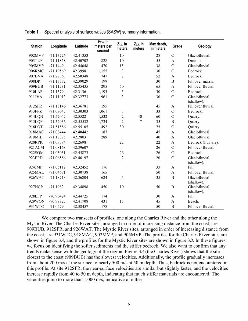
Results Table 1 summarizes the SASW field program. Each tested site is one row, and the columns

include the site code (corresponding to fig. 1), latitude, longitude, average VS to 30-m depth, the depth to the first VS exceeding 1.0 km/s (Z1.0), the depth to the first VS exceeding 2.5 km/s (Z2.5), the maximum depth of the velocity profile (i.e., depth to halfspace), the data/inversion quality grade, and the surface geology category. Note that site 907BVA is adjacent to the strong-motion station at the Bedford VA Hospital (USGS Station 2602), and site 911JVA is located adjacent to the strong-motion station at the Veterans Affairs Hospital in Boston near Jamaica Pond (USGS Station 2649).

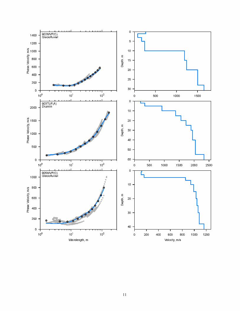
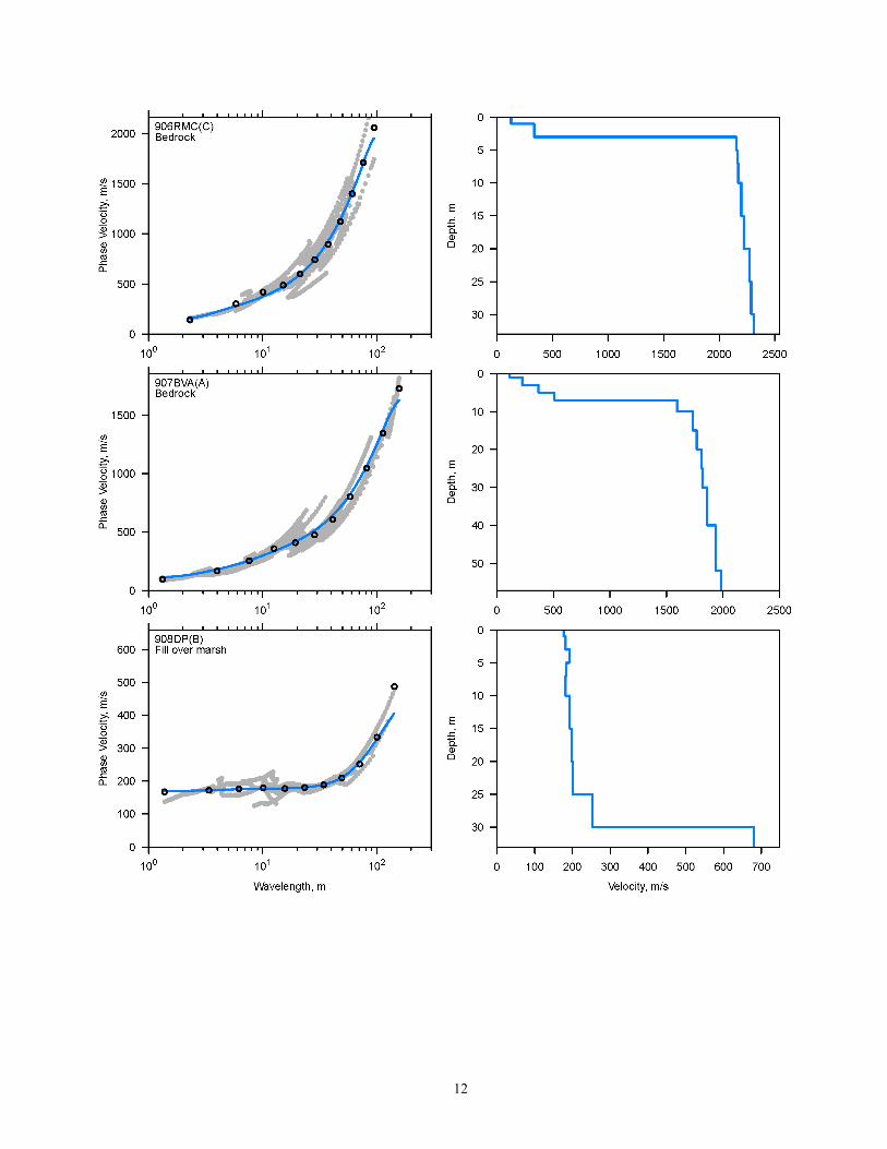
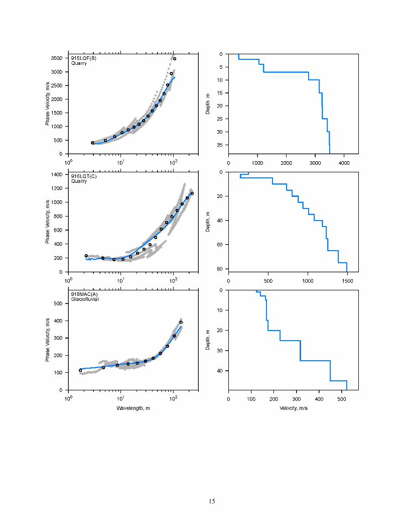
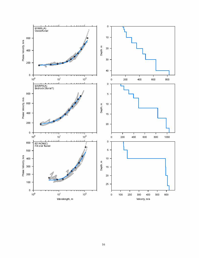
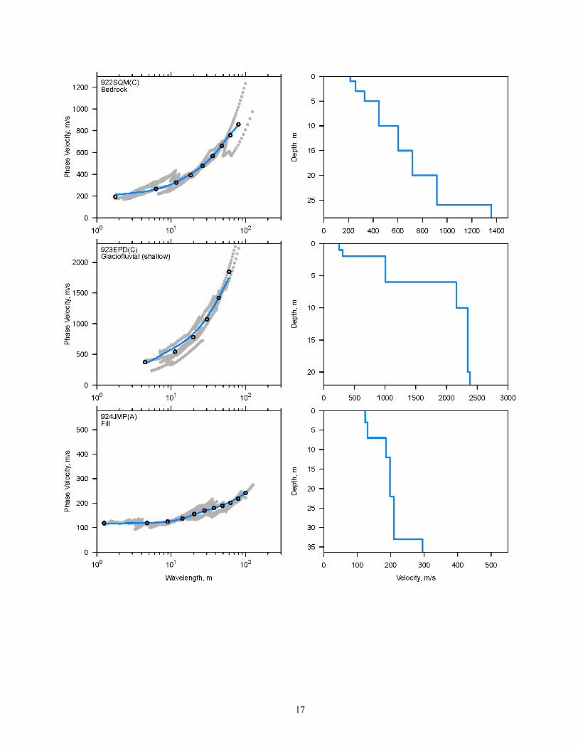
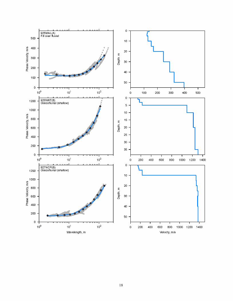
Appendix 1 includes two columns of plots, and each row of plots is for a single site. The left column of plots gives the raw dispersion-curve data, the smoothed averaged dispersion curve, and the theoretical dispersion curve that corresponds to the VS profile at that site. The VS profile is given in the right column of plots. Three pieces of information are given in the upper-left area of the dispersion plots: (1) the site ID, (2) the data/inversion quality grade, and (3) the geologic classification of the site. The data/inversion quality grade is based on consistency of the individual dispersion measurements that were made at the site, the degree of scatter in the dispersion curve, and the ability to find a simple velocity profile that explains the composite dispersion curve.

6

Table 1. Spectral analysis of surface waves (SASW) summary information.

Station Longitude Latitude VS30, in

meters per second

Z1.0, in meters

Z2.5, in meters

Max depth, in meters Grade Geology

902MVP -71.13226 42.41353 10 28 C Glaciofluvial. 903TUF -71.11858 42.40702 828 10 55 A Drumlin. 905MVP -71.1449 42.44048 470 15 38 C Glaciofluvial. 906RMC -71.19569 42.3998 1,155 3 30 C Bedrock. 907BVA -71.27363 42.50348 747 7 52 A Bedrock. 908DP -71.13772 42.39029 199 30 B Fill over marsh. 909BUB -71.11231 42.35435 295 50 65 A Fill over fluvial. 910LAP -71.1379 42.3136 1,193 5 30 C Bedrock. 911JVA -71.11013 42.32773 961 3 30 C Glaciofluvial

(shallow). 912SFR -71.13146 42.36781 195 45 A Fill over fluvial. 913FPZ -71.09047 42.30303 1,061 5 33 C Bedrock. 914LQN -71.52042 42.5522 1,532 2 40 60 C Quarry. 915LQF -71.52036 42.55532 1,734 2 7 35 B Quarry. 916LQT -71.51586 42.55105 492 30 75 C Quarry. 918MAC -71.08444 42.40442 187 45 A Glaciofluvial. 919MIL -71.18375 42.2803 289 40 A Glaciofluvial. 920RPK -71.08384 42.2698 22 22 A Bedrock (fluvial?). 921ACM -71.08168 42.39607 26 C Fill over fluvial. 922SQM -71.03031 42.45873 26 26 C Bedrock. 923EPD -71.06586 42.46197 2 20 C Glaciofluvial

(shallow). 924JMP -71.05112 42.32452 176 33 A Fill. 925MAL -71.04671 42.30738 165 50 A Fill over fluvial. 926WAT -71.18718 42.36804 624 5 35 B Glaciofluvial

(shallow). 927NCP -71.1982 42.34898 450 10 50 B Glaciofluvial

(shallow). 928LFP -70.96424 42.44725 174 30 A Fill. 929WON -70.98927 42.41708 431 15 45 A Beach. 931WTC -71.0579 42.38457 178 50 B Fill over fluvial.

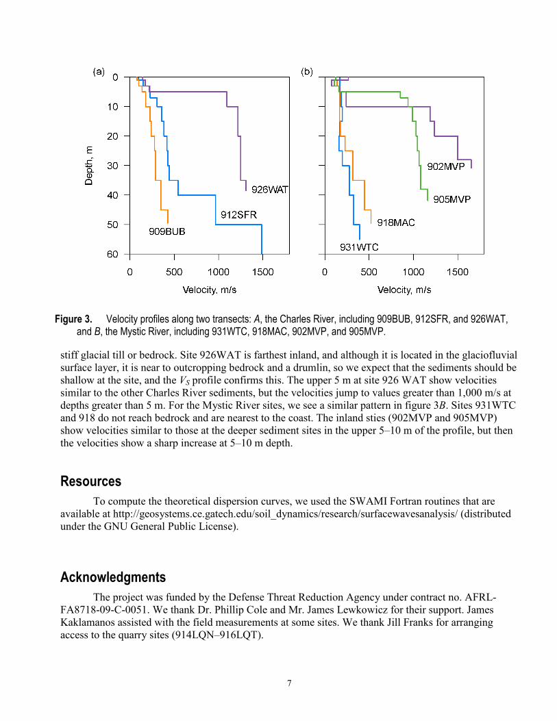
We compare two transects of profiles, one along the Charles River and the other along the

Mystic River. The Charles River sites, arranged in order of increasing distance from the coast, are 909BUB, 912SFR, and 926WAT. The Mystic River sites, arranged in order of increasing distance from the coast, are 931WTC, 918MAC, 902MVP, and 905MVP. The profiles for the Charles River sites are shown in figure 3A, and the profiles for the Mystic River sites are shown in figure 3B. In these figures, we focus on identifying the softer sediments and the stiffer bedrock. We also want to confirm that any trends make sense with the geology of the region. Figure 3A (the Charles River) shows that the site closest to the coast (909BUB) has the slowest velocities. Additionally, the profile gradually increases from about 200 m/s at the surface to nearly 500 m/s at 50 m depth. Thus, bedrock is not encountered in this profile. At site 912SFR, the near-surface velocities are similar but slightly faster, and the velocities increase rapidly from 40 to 50 m depth, indicating that much stiffer materials are encountered. The velocities jump to more than 1,000 m/s, indicative of either

7

Figure 3. Velocity profiles along two transects: A, the Charles River, including 909BUB, 912SFR, and 926WAT, and B, the Mystic River, including 931WTC, 918MAC, 902MVP, and 905MVP.

stiff glacial till or bedrock. Site 926WAT is farthest inland, and although it is located in the glaciofluvial surface layer, it is near to outcropping bedrock and a drumlin, so we expect that the sediments should be shallow at the site, and the VS profile confirms this. The upper 5 m at site 926 WAT show velocities similar to the other Charles River sediments, but the velocities jump to values greater than 1,000 m/s at depths greater than 5 m. For the Mystic River sites, we see a similar pattern in figure 3B. Sites 931WTC and 918 do not reach bedrock and are nearest to the coast. The inland sties (902MVP and 905MVP) show velocities similar to those at the deeper sediment sites in the upper 5–10 m of the profile, but then the velocities show a sharp increase at 5–10 m depth.

Resources To compute the theoretical dispersion curves, we used the SWAMI Fortran routines that are

available at http://geosystems.ce.gatech.edu/soil_dynamics/research/surfacewavesanalysis/ (distributed under the GNU General Public License).

Acknowledgments The project was funded by the Defense Threat Reduction Agency under contract no. AFRL-

FA8718-09-C-0051. We thank Dr. Phillip Cole and Mr. James Lewkowicz for their support. James Kaklamanos assisted with the field measurements at some sites. We thank Jill Franks for arranging access to the quarry sites (914LQN–916LQT).

8

References Cited Atkinson, G.M., and Boore, D.M., Earthquake ground-motion prediction equations for eastern North

America: Bulletin of the Seismological Society of America, v. 96, p. 2181–2205. Barosh, P.J., Kaye, C.A., and Woodhouse, D., 1989, Geology of the Boston basin & vicinity, Civil

Engineering Practice, v. 4, p. 39–52. Britton, J.M., 2003, Microzonation of the Boston area, MS Thesis, Department of Geology and

Geophysics, Boston College, 58 p. Boore, D.M., Campbell, K.W., and Atkinson, G.M., 2010, Determination of stress parameters for eight

well-recorded earthquakes in eastern North America, Bulletin of the Seismological Society of America, v. 100, p. 1632–1645.

Brankman, C.M., and Baise, L.G., 2008, Liquefaction susceptibility mapping in Boston, Massachusetts: Environmental and Engineering Geoscience, v. 14, p. 1–16.

Ebel, J.E., 1996, The seventeenth century seismicity of northeastern North America: Seismological Research Letters, v. 67, p. 51–68.

Ebel, J.E., 2006, The Cape Ann, Massachusetts, earthquake of 1755—A 250th anniversary perspective: Seismological Research Letters, 77, 74–86.

Ebel, J.E., and Hart, K.A., 2001, Observational evidence for amplification of earthquake ground motions in Boston and Vicinity: Civil Engineering Practice, v. 16, p. 5–16.

Ebel, J.E., and W-Y. Kim, 2006, Shake maps for earthquakes in the northeastern United States: collaborative research with Columbia University and Boston College, Final Technical Report for USGS Awards 06HQGR0019 and 06HQGR0022.

Frankel, A., 1991, Mechanisms of seismic attenuation in the crust scattering and anelasticity in New York State, South Africa, and southern California: Journal of Geophysical Research, v. 96, p. 6269–6289.

Hayles, K.E., Ebel, J.E., and Urzua, A., 2001, Microtremor measurements to obtain resonant frequencies and ground shaking amplification for soil sites in Boston: Civil Engineering Practice, v. 16, p. 17–36.

Johnson, E.G., 1989, Geotechnical characteristics of the Boston area: Civil Engineering Practice, v. ???, p. 53–64.

Kaye, C.A., 1982, Bedrock and Quaternary geology of the Boston area, Massachusetts, Geological Society of America Reviews in Engineering Geology, 5, 25–40.

Kummer, K.E., 1998, Microtremor measurements to obtain resonant frequencies and ground shaking amplification for soil sites in Boston, MA: MS Thesis, Department of Geology and Geophysics, Boston College, 163 p.

Lai, C.G., and Rix, G.J., 1998, Simultaneous Inversion of Rayleigh Phase Velocity and Attenuation for Near-Surface Site Characterization, Report No. GIT-CEE/GEO-98-2: Georgia Institute of Technology, School of Civil and Environmental Engineering, 258 p.

Schnabel, P.B., Lysmer, J., and Seed, H.B., 1972, SHAKE: A computer program for earthquake response analysis of horizontally layered sites, Technical Report Rept. EERC 72–12, Earthquake Engineering Research Center, University of California, Berkeley.

Somerville, P.G., McLaren, J.P., LeFevre, L.V., Burger, R.W., and Helmberger D.V., 1987, Comparison of source scaling relations of eastern and western North American earthquakes: Bulletin of the Seismological Society of America, v. 77, p. 332–346.

Street, R., and Lacroix, A., 1979, An empirical study of New England seismicity: 1727–1977: Bulletin of the Seismological Society of America, v. 69, p. 159–175.

9

Tavakoli, B., and Pezeshk, S., 2005, Empirical-stochastic ground-motion prediction for eastern North America: Bulletin of the Seismological Society of America, v. 95, p. 2283–2296.

Viegas, G.M., Baise, L.G., and Abercrombie, R.E., 2010, Regional Wave Propagation in New England and New York: Bulletin of the Seismological Society of America, v. 100, p. 2196–2218.

Wald, D.J., Allen, T.I., 2007, Topographic Slope as a Proxy for Seismic Site Conditions and Amplification, Bulletin of the Seismological Society of America, v. 97, p. 1379–1395.

Woodhouse, D., Barosh, P.J., Johnson, E.G., Kaye, C.A., Russell, H.A., Pitt, W.E., Jr., Alsup, S.A., and Franz, K.E., 1991, Geology of Boston, Massachusetts, United States of America: Bulletin Association of Engineering Geologists, v. 28, p. 375–512.

10

Appendix 1. Shear-Wave Velocity Profiles

11

12

13

14

15

16

17

18

19

Appendix 2. Site Descriptions

Figure A1. Photos of site 902MVP, in a parking lot along Mystic Valley Parkway, near Boston, Massachusetts.

Figure A2. Photos of site 903TUF, in the quad of Tufts University, near Boston, Mass.

Figure A3. Photos of site 905MVP, on the east side of Upper Mystic Lake, near Boston, Mass.

20

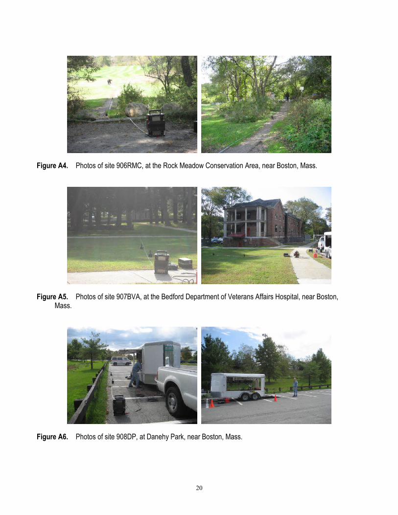
Figure A4. Photos of site 906RMC, at the Rock Meadow Conservation Area, near Boston, Mass.

Figure A5. Photos of site 907BVA, at the Bedford Department of Veterans Affairs Hospital, near Boston, Mass.

Figure A6. Photos of site 908DP, at Danehy Park, near Boston, Mass.

21

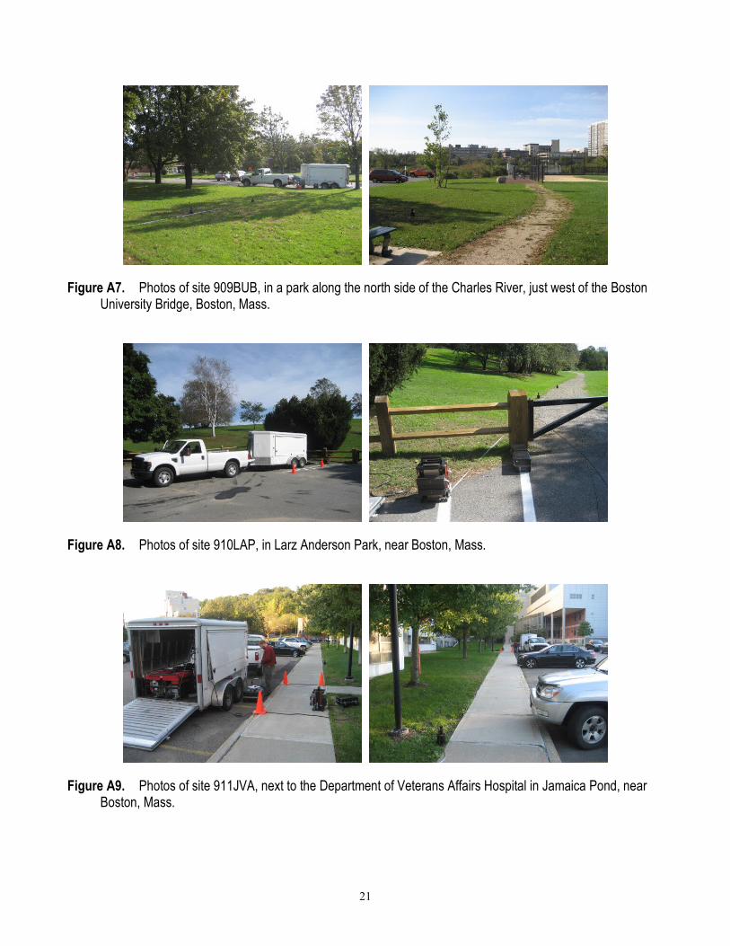
Figure A7. Photos of site 909BUB, in a park along the north side of the Charles River, just west of the Boston University Bridge, Boston, Mass.

Figure A8. Photos of site 910LAP, in Larz Anderson Park, near Boston, Mass.

Figure A9. Photos of site 911JVA, next to the Department of Veterans Affairs Hospital in Jamaica Pond, near Boston, Mass.

22

Figure A10. Photos of site 912SFR, off of Soldiers Field Road, just south of Eliot Bridge, near Boston, Mass.

Figure A11. Photos of site 913FPZ, next to the Franklin Park Zoo, near Boston, Mass.

Figure A12. Photos of site 914LQN, in Littleton, Mass.

23

Figure A13. Photos of site 915LQF, in Littleton, Mass.

Figure A14. Photos of site 916LQT, in Littleton, Mass.

Figure A15. Photos of site 918MAC, in Macdonald Park, near Boston, Mass.

24

Figure A16. Photos of site 919MIL, in Millenium Park, near Boston, Mass.

Figure A17. Photos of site 920RPK, in Ryan Park, near Boston, Mass.

Figure A18. Photos of site 921ACM, along the Mystic River in the parking lot of Assembly Square Mall, near Boston, Mass.

25

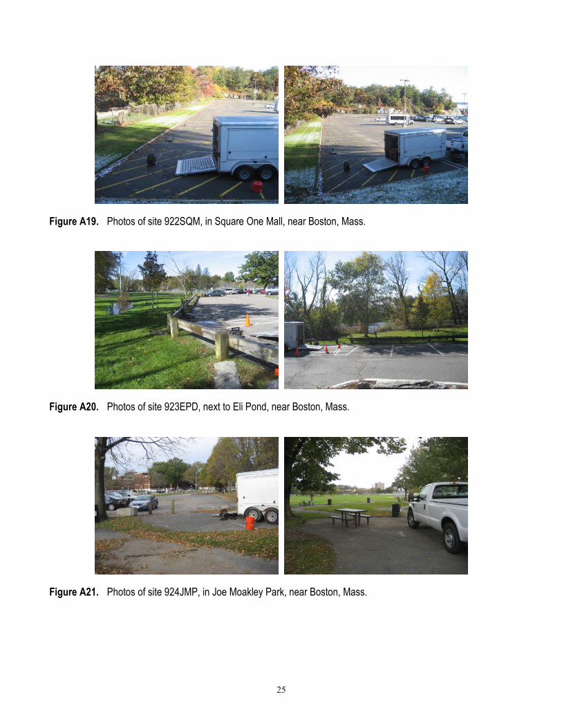
Figure A19. Photos of site 922SQM, in Square One Mall, near Boston, Mass.

Figure A20. Photos of site 923EPD, next to Eli Pond, near Boston, Mass.

Figure A21. Photos of site 924JMP, in Joe Moakley Park, near Boston, Mass.

26

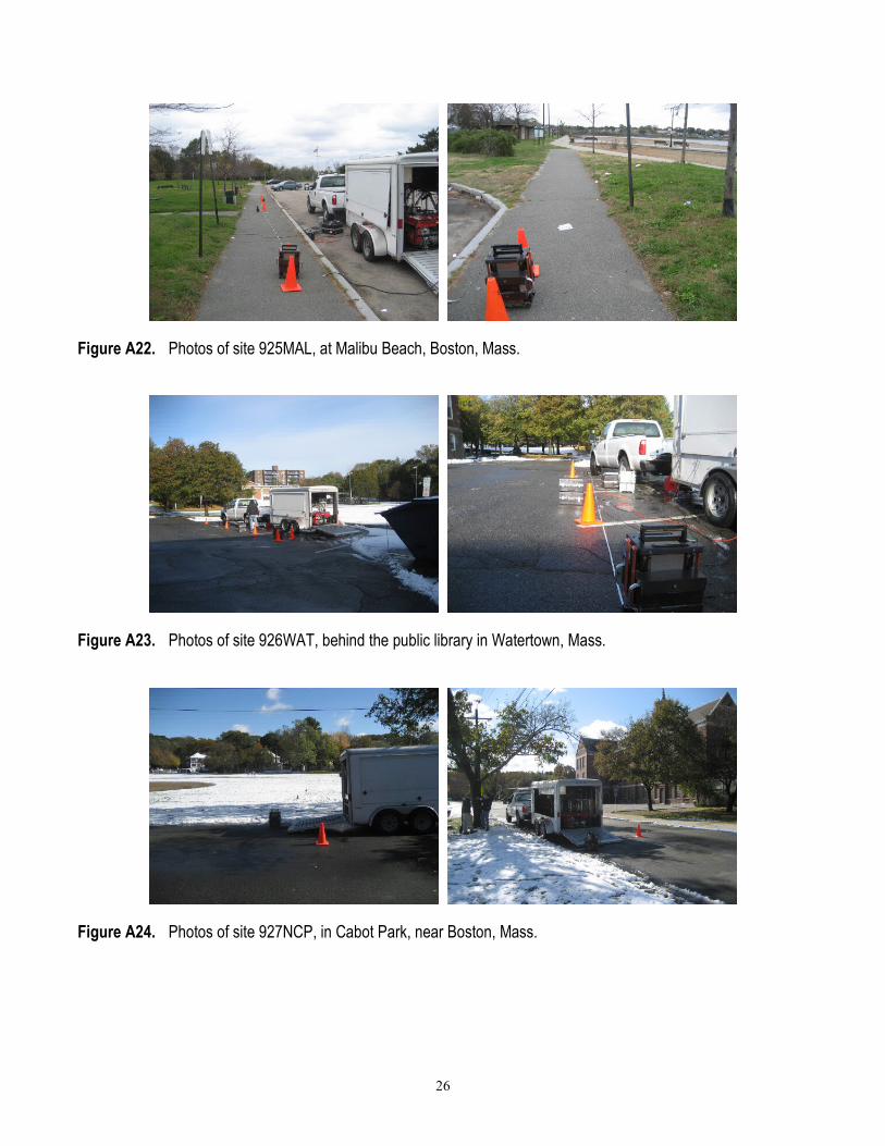
Figure A22. Photos of site 925MAL, at Malibu Beach, Boston, Mass.

Figure A23. Photos of site 926WAT, behind the public library in Watertown, Mass.

Figure A24. Photos of site 927NCP, in Cabot Park, near Boston, Mass.

27

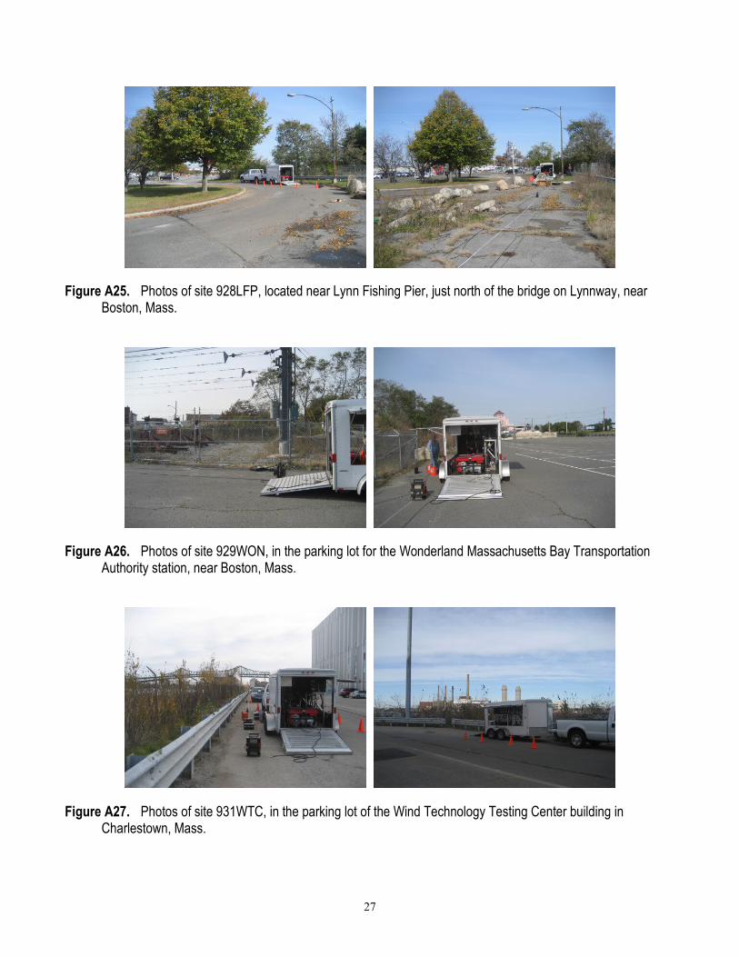
Figure A25. Photos of site 928LFP, located near Lynn Fishing Pier, just north of the bridge on Lynnway, near Boston, Mass.

Figure A26. Photos of site 929WON, in the parking lot for the Wonderland Massachusetts Bay Transportation Authority station, near Boston, Mass.

Figure A27. Photos of site 931WTC, in the parking lot of the Wind Technology Testing Center building in Charlestown, Mass.