Supply Chain Disruptions Preparedness Measures Using a Dynamic Model

_________________________________________________________________________

Abstract:

Supply chain risk management has recently seen extensive research efforts, but questions such as

“How should a firm plan for each type of disruption?” and “What are the strategies and the total

cost incurred by the firm if a disruption occurs?” continue to deserve attention. This chapter

analyzes different disruption cases by considering the impacts of disruptions at a supplier, a firm’s

warehouse, and at the firm’s production facility. The firm can prepare for each type of disruption

by buying from an alternate supplier, holding more inventory, or holding inventory at a different

warehouse. The Wagner-Whitin model is used to solve the optimal ordering strategy for each type

of disruption. Since the type of disruption is uncertain, we assign probabilities for each disruption

and use the Wagner-Whitin model to find the order policy that minimizes the firm’s expected cost.

Keywords: Supply chain disruption, preparedness, Wagner-Whitin Model.

1. Introduction

Disruptions are unpredictable events and can occur at any facility location of a plant at any point

of time. A supply chain is vulnerable to different types of disruptions, which can take the form of

supply disruptions, operational problems at warehouses, demand uncertainty, transportation

difficulties, or catastrophic events that close a firm’s manufacturing facilities. Since a firm does

not know what type of disruption will occur, if any, planning for disruptions should account for

this uncertainty.

This chapter addresses disruptions occurring at three major locations: a supplier, a warehouse,

and a firm’s production facility. Two important questions are: (1) How should a firm plan for each

type of disruption? and (2) How should a firm prepare for the possibility of all three disruptions?

This chapter presents a model that seeks to answer these questions by exploring the firm’s planning

horizon and preparation strategies. First, the firm can prepare itself from calamity by holding

inventory, possibly at different locations. Second, the firm can have an alternate supplier for its

product.

Preparation strategies may also account for how the firm and other entities may respond if a

disruption occurs. For example, a multinational firm may be able to rely on suppliers from other

countries that are not impacted by a disruption. For example, if the firm’s manufacturing plant is

located in one part of world, the firm could increase productions at other facilities. Selecting

international suppliers as an alternate supplier may incur higher ordering cost, however.

Each of the preparation strategies has a cost, and the cost of implementing all these strategies

might be higher than the disruption itself. This chapter models this decision using the Wagner-

Whitin model to incorporate the uncertainty around the type of disruption and to select a strategy

that minimizes the firm’s expected cost. This research is novel because we look at preparedness

strategies of a firm during disruptions, which will reduce the overall disruption losses. It uses the

idea of the Wagner-Whitin model to think about different disruption scenarios. A firm can use this

Wagner-Whitin model with disruptions to make profitable decisions before and after a disruption.

Section 2 reviews the literature on supply chain disruptions. Section 3 introduces the supply

chain model, the Wagner-Whitin algorithm, and the three disruption scenarios. Section 4 applies

probabilities to each disruption and finds the firm’s order policy that minimizes its expected cost.

Section 5 discusses the results of this analysis.

2. Literature Review

Supply chain risk management and supply chain disruptions have received a lot of attention

both in academia and in industry. A supply chain disruption can be defined as an internal or

external event that alters the normal or planned flow of goods and services in a supply chain.

Literature reviews on supply chain disruptions and supply chain risk management can be found in

Tang (2006), Snyder et al. (2006), Vakharia and Yeniparzarli (2008), Natarajarathinam et al.

(2009), Schmitt and Tomlin (2012), and Snyder et al. (2016). Supply chain disruptions can take

many different forms, including production difficulties or operational risks (Xia et al., 2004),

wholesale prices impacted by cost fluctuations (Xiao and Qi, 2008), supply shortages (Xiao and

Yu, 2006), and sudden drops in demand based on the market conditions (Xiao et al., 2005). Much

of the academic literature on supply chain disruptions focuses on understanding and modeling

strategies that firms can use to mitigate a disruption, such as holding inventory (Song and Zipkin,

1996; Tomlin, 2006) purchasing from alternate suppliers (Tomlin, 2006; Song and Zipkin, 2009;

Babich et al., 2007; Hopp et al., 2009), rescheduling production (Bean et al., 1991; Adhyitya et

al., 2007), rerouting transportation (MacKenzie et al., 2012), and producing at an alternate facility

(MacKenzie et al., 2014). A firm can attempt to build a supply chain resilient to disruptions (Sheffi,

2005) by reconfiguring resources or improving its infrastructure (Ambulkar et al., 2015).

Understanding characteristics that make firms more or less vulnerable to supply chain

disruptions is another important area of research. Bode and Wagner (2015) empirically found that

the complexity of a supply chain, to include the horizontal and vertical complexity, can increase

the frequency of disruptions and exacerbate them. Make-to-order supply chains may be more

vulnerable to disruptions than make-to-forecast supply chains (Papadakis, 2006). Supply chain

disruptions may be more severe for firms that are more geographically diverse or undertake a lot

of outsourcing (Hendricks et al., 2009). This chapter explores some of the potential impacts that

could occur in a complex supply chain with multiple suppliers and different warehouses.

The model in this chapter uses the model developed by Wagner and Whitin (1958) which

provides a production or ordering plan with varying but known demand. If demand and order lead

time are uncertain to small extent, a modified Wagner-Whitin model can still be applied (Kazan et

al., 2000; Jeunet and Jonard, 2000). The Wagner-Whitin model was recently extended to situations

with variable manufacturing and remanufacturing cost (Richter and Sombrutzki, 2000; Richter and

Weber, 2001). To our knowledge, no research has extended the Wagner-Whitin model to supply

chain disruptions to understand how a firm can use a manufacturing resource planning system to

prepare for potential disruptions.

3. Supply Chain Model and Illustrative Example

3.1 Model

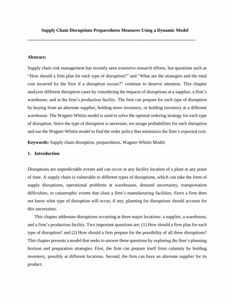
We consider a supply chain (see Figure 1) in which a manufacturing firm requires several

suppliers. These suppliers transform raw materials into goods that are delivered to the firm. The

firm stores these supplies in a warehouse. The firm also operates two smaller warehouses that are

located further away but can be used if the main warehouse is short of supplies or unusable. The

firm depends on a single primary supplier for parts. An alternate supplier is also available to deliver

parts at a more expensive price if the primary supplier cannot meet demand. Since this chapter

assumes that at most one supplier is disrupted, the analysis focuses on the firm’s ability to obtain

parts for its manufacturing process.

Figure 1: Supply chain map

We assume that the firm’s forecasted demand 𝐷𝑡 in time period 𝑡 is deterministic but changes

in each time period where 𝑡 = 1,2, … , 𝑇 and 𝑇 represents the planning horizon. The firm develops

a plan to order quantity 𝑄𝑡 in each period in order to minimize its cumulative cost over the time

horizon. The firm’s cost is composed of a per-unit ordering cost 𝐶𝑡, a fixed cost per order 𝐴𝑡, and

a per-unit holding or inventory cost 𝐻𝑡. All costs are in U.S. dollars. Given the assumptions in this

framework, the model developed by Wagner and Whitin (1958) provides an appropriate solution

for the firm’s planning. The Wagner-Whitin model is a dynamic lot-sizing model that produces an

optimal lot size for each period. A notional example is developed for a firm using the “RoadHog”

example from Hopp and Spearman (pp. 58-64, 2008). The example without a disruption is

explained first. We extend the example to three possible scenario disruptions: (1) a supplier

disruption, (2) a firm closure, and (3) a warehouse disruption.

3.2 No Disruptions

Table 1 depicts the parameters for a 10-period model. The demand changes in each period, but

the variable ordering cost, the fixed order cost, and the holding cost remain the same for each

period. The cost in period 𝑡 equals 𝐴𝑡1𝑄𝑡>0 + 𝐶𝑡𝑄𝑡 + 𝐻𝑡𝐼𝑡 where 1𝑄𝑡>0 is in the indicator function

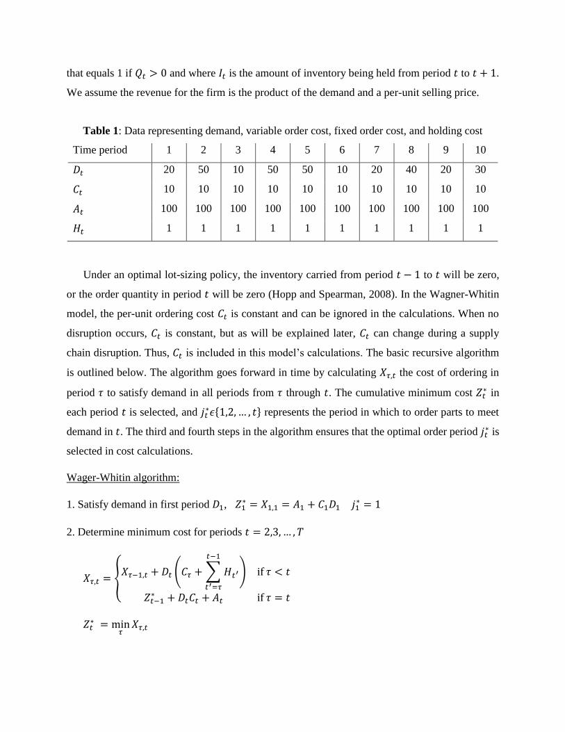
that equals 1 if 𝑄𝑡 > 0 and where 𝐼𝑡 is the amount of inventory being held from period 𝑡 to 𝑡 + 1.

We assume the revenue for the firm is the product of the demand and a per-unit selling price.

Table 1: Data representing demand, variable order cost, fixed order cost, and holding cost

Time period 1 2 3 4 5 6 7 8 9 10

𝐷𝑡 20 50 10 50 50 10 20 40 20 30

𝐶𝑡 10 10 10 10 10 10 10 10 10 10

𝐴𝑡 100 100 100 100 100 100 100 100 100 100

𝐻𝑡 1 1 1 1 1 1 1 1 1 1

Under an optimal lot-sizing policy, the inventory carried from period 𝑡 − 1 to 𝑡 will be zero,

or the order quantity in period 𝑡 will be zero (Hopp and Spearman, 2008). In the Wagner-Whitin

model, the per-unit ordering cost 𝐶𝑡 is constant and can be ignored in the calculations. When no

disruption occurs, 𝐶𝑡 is constant, but as will be explained later, 𝐶𝑡 can change during a supply

chain disruption. Thus, 𝐶𝑡 is included in this model’s calculations. The basic recursive algorithm

is outlined below. The algorithm goes forward in time by calculating 𝑋𝜏,𝑡 the cost of ordering in

period 𝜏 to satisfy demand in all periods from 𝜏 through 𝑡. The cumulative minimum cost 𝑍𝑡∗ in

each period 𝑡 is selected, and 𝑗𝑡∗𝜖{1,2, … , 𝑡} represents the period in which to order parts to meet

demand in 𝑡. The third and fourth steps in the algorithm ensures that the optimal order period 𝑗𝑡∗ is

selected in cost calculations.

Wager-Whitin algorithm:

1. Satisfy demand in first period 𝐷1, 𝑍1∗ = 𝑋1,1 = 𝐴1 + 𝐶1𝐷1 𝑗1

∗ = 1

2. Determine minimum cost for periods 𝑡 = 2,3, … , 𝑇

𝑋𝜏,𝑡 = {𝑋𝜏−1,𝑡 + 𝐷𝑡 (𝐶𝜏 + ∑ 𝐻𝑡′

𝑡−1

𝑡′=𝜏

) if 𝜏 < 𝑡

𝑍𝑡−1∗ + 𝐷𝑡𝐶𝑡 + 𝐴𝑡 if 𝜏 = 𝑡

𝑍𝑡∗ = min

𝜏𝑋𝜏,𝑡

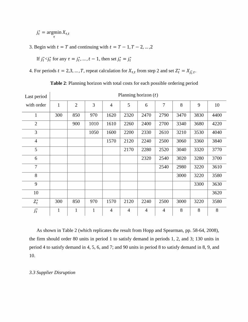
𝑗𝑡∗ = argmin

𝜏𝑋𝜏,𝑡

3. Begin with 𝑡 = 𝑇 and continuing with 𝑡 = 𝑇 − 1, 𝑇 − 2, … ,2

If 𝑗𝑡∗<𝑗𝜏

∗ for any 𝜏 = 𝑗𝑡∗, … , 𝑡 − 1, then set 𝑗𝜏

∗ = 𝑗𝑡∗

4. For periods 𝑡 = 2,3, … , 𝑇, repeat calculation for 𝑋𝜏,𝑡 from step 2 and set 𝑍𝑡∗ = 𝑋𝑗𝑡

∗,𝑡.

Table 2: Planning horizon with total costs for each possible ordering period

Last period

with order

Planning horizon (𝑡)

1 2 3 4 5 6 7 8 9 10

1 300 850 970 1620 2320 2470 2790 3470 3830 4400

2 900 1010 1610 2260 2400 2700 3340 3680 4220

3 1050 1600 2200 2330 2610 3210 3530 4040

4 1570 2120 2240 2500 3060 3360 3840

5 2170 2280 2520 3040 3320 3770

6 2320 2540 3020 3280 3700

7 2540 2980 3220 3610

8 3000 3220 3580

9 3300 3630

10 3620

𝑍𝑡∗ 300 850 970 1570 2120 2240 2500 3000 3220 3580

𝑗𝑡∗ 1 1 1 4 4 4 4 8 8 8

As shown in Table 2 (which replicates the result from Hopp and Spearman, pp. 58-64, 2008),

the firm should order 80 units in period 1 to satisfy demand in periods 1, 2, and 3; 130 units in

period 4 to satisfy demand in 4, 5, 6, and 7; and 90 units in period 8 to satisfy demand in 8, 9, and

10.

3.3 Supplier Disruption

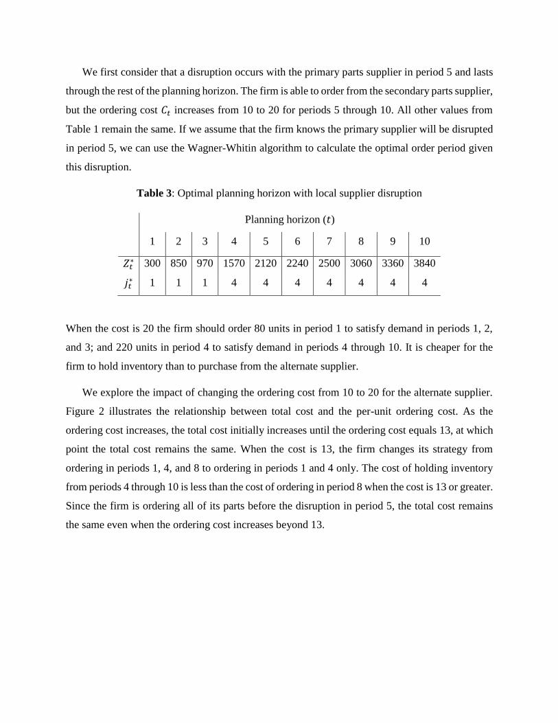
We first consider that a disruption occurs with the primary parts supplier in period 5 and lasts

through the rest of the planning horizon. The firm is able to order from the secondary parts supplier,

but the ordering cost 𝐶𝑡 increases from 10 to 20 for periods 5 through 10. All other values from

Table 1 remain the same. If we assume that the firm knows the primary supplier will be disrupted

in period 5, we can use the Wagner-Whitin algorithm to calculate the optimal order period given

this disruption.

Table 3: Optimal planning horizon with local supplier disruption

Planning horizon (𝑡)

1 2 3 4 5 6 7 8 9 10

𝑍𝑡∗ 300 850 970 1570 2120 2240 2500 3060 3360 3840

𝑗𝑡∗ 1 1 1 4 4 4 4 4 4 4

When the cost is 20 the firm should order 80 units in period 1 to satisfy demand in periods 1, 2,

and 3; and 220 units in period 4 to satisfy demand in periods 4 through 10. It is cheaper for the

firm to hold inventory than to purchase from the alternate supplier.

We explore the impact of changing the ordering cost from 10 to 20 for the alternate supplier.

Figure 2 illustrates the relationship between total cost and the per-unit ordering cost. As the

ordering cost increases, the total cost initially increases until the ordering cost equals 13, at which

point the total cost remains the same. When the cost is 13, the firm changes its strategy from

ordering in periods 1, 4, and 8 to ordering in periods 1 and 4 only. The cost of holding inventory

from periods 4 through 10 is less than the cost of ordering in period 8 when the cost is 13 or greater.

Since the firm is ordering all of its parts before the disruption in period 5, the total cost remains

the same even when the ordering cost increases beyond 13.

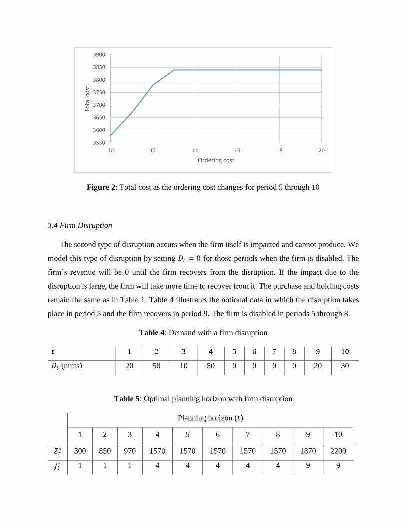
Figure 2: Total cost as the ordering cost changes for period 5 through 10

3.4 Firm Disruption

The second type of disruption occurs when the firm itself is impacted and cannot produce. We

model this type of disruption by setting 𝐷𝑡 = 0 for those periods when the firm is disabled. The

firm’s revenue will be 0 until the firm recovers from the disruption. If the impact due to the

disruption is large, the firm will take more time to recover from it. The purchase and holding costs

remain the same as in Table 1. Table 4 illustrates the notional data in which the disruption takes

place in period 5 and the firm recovers in period 9. The firm is disabled in periods 5 through 8.

Table 4: Demand with a firm disruption

𝑡 1 2 3 4 5 6 7 8 9 10

𝐷𝑡 (units) 20 50 10 50 0 0 0 0 20 30

Table 5: Optimal planning horizon with firm disruption

Planning horizon (𝑡)

1 2 3 4 5 6 7 8 9 10

𝑍𝑡∗ 300 850 970 1570 1570 1570 1570 1570 1870 2200

𝑗𝑡∗ 1 1 1 4 4 4 4 4 9 9

3550

3600

3650

3700

3750

3800

3850

3900

10 12 14 16 18 20

Tota

l co

st

Ordering cost

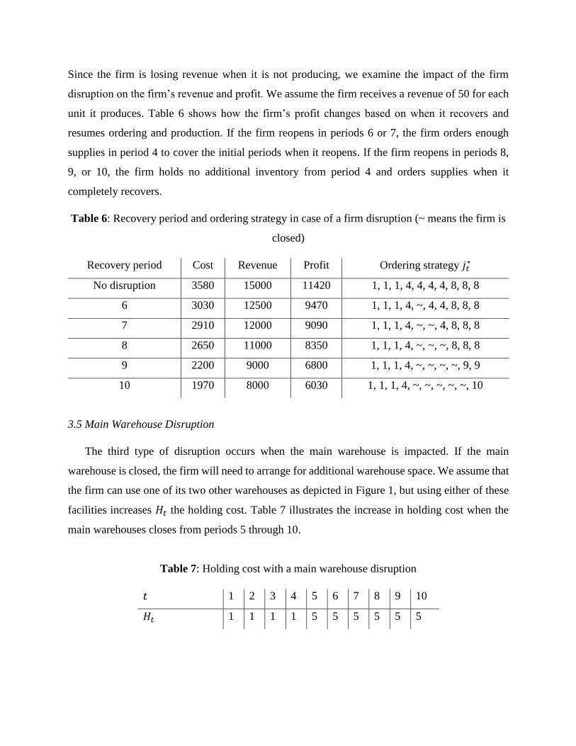
Since the firm is losing revenue when it is not producing, we examine the impact of the firm

disruption on the firm’s revenue and profit. We assume the firm receives a revenue of 50 for each

unit it produces. Table 6 shows how the firm’s profit changes based on when it recovers and

resumes ordering and production. If the firm reopens in periods 6 or 7, the firm orders enough

supplies in period 4 to cover the initial periods when it reopens. If the firm reopens in periods 8,

9, or 10, the firm holds no additional inventory from period 4 and orders supplies when it

completely recovers.

Table 6: Recovery period and ordering strategy in case of a firm disruption (~ means the firm is

closed)

Recovery period Cost Revenue Profit Ordering strategy 𝑗𝑡∗

No disruption 3580 15000 11420 1, 1, 1, 4, 4, 4, 4, 8, 8, 8

6 3030 12500 9470 1, 1, 1, 4, ~, 4, 4, 8, 8, 8

7 2910 12000 9090 1, 1, 1, 4, ~, ~, 4, 8, 8, 8

8 2650 11000 8350 1, 1, 1, 4, ~, ~, ~, 8, 8, 8

9 2200 9000 6800 1, 1, 1, 4, ~, ~, ~, ~, 9, 9

10 1970 8000 6030 1, 1, 1, 4, ~, ~, ~, ~, ~, 10

3.5 Main Warehouse Disruption

The third type of disruption occurs when the main warehouse is impacted. If the main

warehouse is closed, the firm will need to arrange for additional warehouse space. We assume that

the firm can use one of its two other warehouses as depicted in Figure 1, but using either of these

facilities increases 𝐻𝑡 the holding cost. Table 7 illustrates the increase in holding cost when the

main warehouses closes from periods 5 through 10.

Table 7: Holding cost with a main warehouse disruption

𝑡 1 2 3 4 5 6 7 8 9 10

𝐻𝑡 1 1 1 1 5 5 5 5 5 5

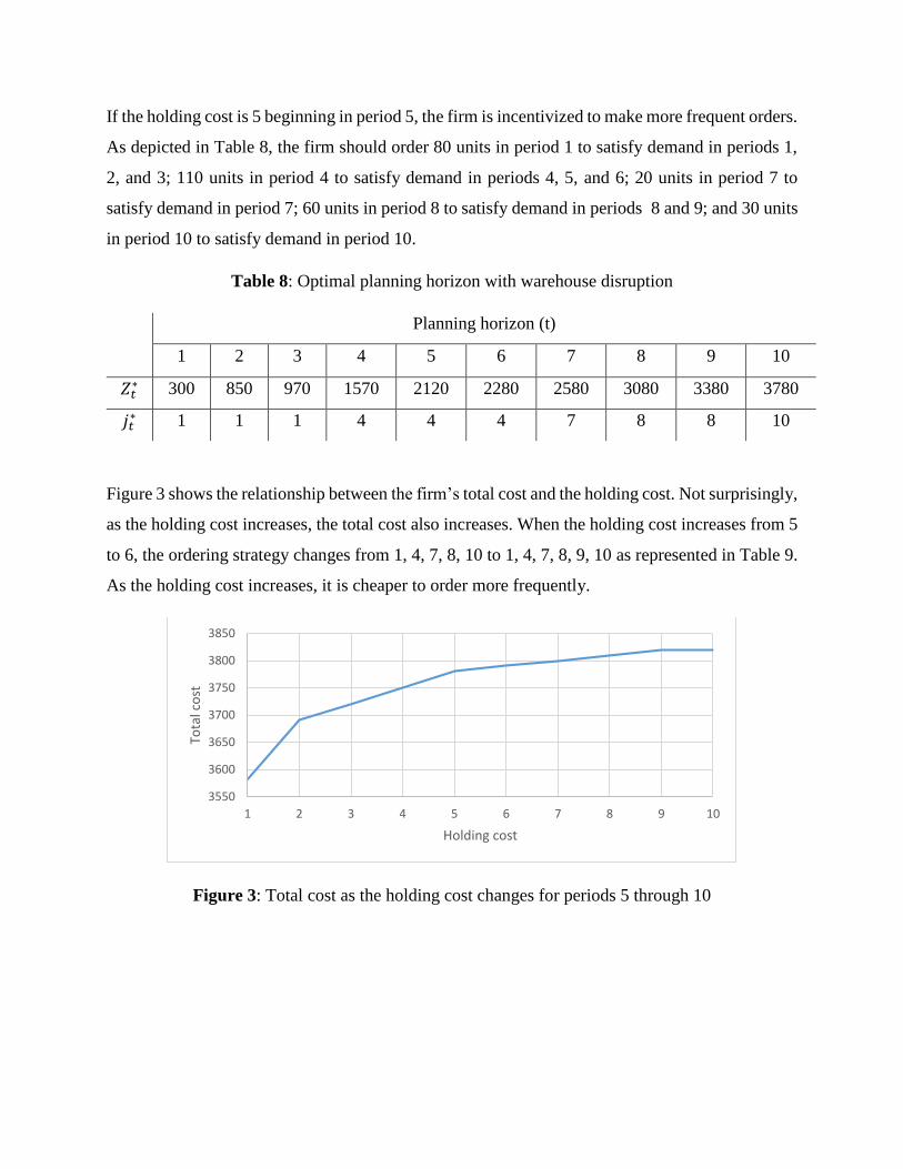
If the holding cost is 5 beginning in period 5, the firm is incentivized to make more frequent orders.

As depicted in Table 8, the firm should order 80 units in period 1 to satisfy demand in periods 1,

2, and 3; 110 units in period 4 to satisfy demand in periods 4, 5, and 6; 20 units in period 7 to

satisfy demand in period 7; 60 units in period 8 to satisfy demand in periods 8 and 9; and 30 units

in period 10 to satisfy demand in period 10.

Table 8: Optimal planning horizon with warehouse disruption

Planning horizon (t)

1 2 3 4 5 6 7 8 9 10

𝑍𝑡∗ 300 850 970 1570 2120 2280 2580 3080 3380 3780

𝑗𝑡∗ 1 1 1 4 4 4 7 8 8 10

Figure 3 shows the relationship between the firm’s total cost and the holding cost. Not surprisingly,

as the holding cost increases, the total cost also increases. When the holding cost increases from 5

to 6, the ordering strategy changes from 1, 4, 7, 8, 10 to 1, 4, 7, 8, 9, 10 as represented in Table 9.

As the holding cost increases, it is cheaper to order more frequently.

Figure 3: Total cost as the holding cost changes for periods 5 through 10

3550

3600

3650

3700

3750

3800

3850

1 2 3 4 5 6 7 8 9 10

Tota

l co

st

Holding cost

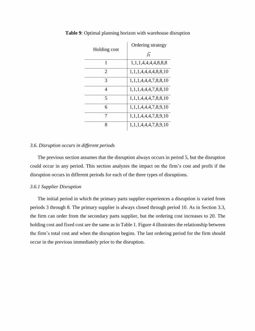
Table 9: Optimal planning horizon with warehouse disruption

Holding cost Ordering strategy

𝑗𝑡∗

1 1,1,1,4,4,4,4,8,8,8

2 1,1,1,4,4,4,4,8,8,10

3 1,1,1,4,4,4,7,8,8,10

4 1,1,1,4,4,4,7,8,8,10

5 1,1,1,4,4,4,7,8,8,10

6 1,1,1,4,4,4,7,8,9,10

7 1,1,1,4,4,4,7,8,9,10

8 1,1,1,4,4,4,7,8,9,10

3.6. Disruption occurs in different periods

The previous section assumes that the disruption always occurs in period 5, but the disruption

could occur in any period. This section analyzes the impact on the firm’s cost and profit if the

disruption occurs in different periods for each of the three types of disruptions.

3.6.1 Supplier Disruption

The initial period in which the primary parts supplier experiences a disruption is varied from

periods 3 through 8. The primary supplier is always closed through period 10. As in Section 3.3,

the firm can order from the secondary parts supplier, but the ordering cost increases to 20. The

holding cost and fixed cost are the same as in Table 1. Figure 4 illustrates the relationship between

the firm’s total cost and when the disruption begins. The last ordering period for the firm should

occur in the previous immediately prior to the disruption.

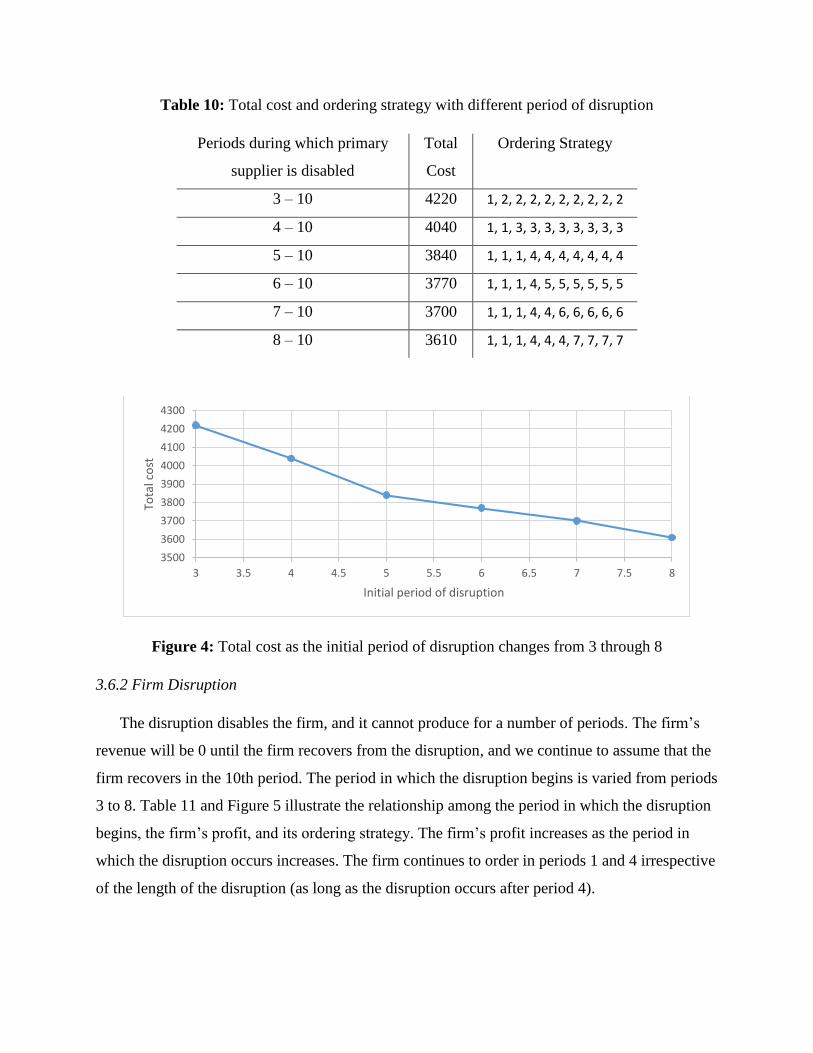
Table 10: Total cost and ordering strategy with different period of disruption

Periods during which primary

supplier is disabled

Total

Cost

Ordering Strategy

3 – 10 4220 1, 2, 2, 2, 2, 2, 2, 2, 2, 2

4 – 10 4040 1, 1, 3, 3, 3, 3, 3, 3, 3, 3

5 – 10 3840 1, 1, 1, 4, 4, 4, 4, 4, 4, 4

6 – 10 3770 1, 1, 1, 4, 5, 5, 5, 5, 5, 5

7 – 10 3700 1, 1, 1, 4, 4, 6, 6, 6, 6, 6

8 – 10 3610 1, 1, 1, 4, 4, 4, 7, 7, 7, 7

Figure 4: Total cost as the initial period of disruption changes from 3 through 8

3.6.2 Firm Disruption

The disruption disables the firm, and it cannot produce for a number of periods. The firm’s

revenue will be 0 until the firm recovers from the disruption, and we continue to assume that the

firm recovers in the 10th period. The period in which the disruption begins is varied from periods

3 to 8. Table 11 and Figure 5 illustrate the relationship among the period in which the disruption

begins, the firm’s profit, and its ordering strategy. The firm’s profit increases as the period in

which the disruption occurs increases. The firm continues to order in periods 1 and 4 irrespective

of the length of the disruption (as long as the disruption occurs after period 4).

3500

3600

3700

3800

3900

4000

4100

4200

4300

3 3.5 4 4.5 5 5.5 6 6.5 7 7.5 8

Tota

l co

st

Initial period of disruption

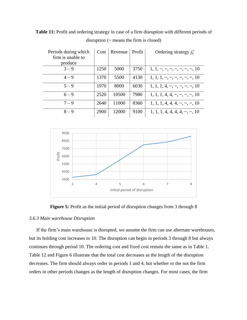
Table 11: Profit and ordering strategy in case of a firm disruption with different periods of

disruption (~ means the firm is closed)

Periods during which

firm is unable to

produce

Cost Revenue Profit Ordering strategy 𝑗𝑡∗

3 – 9 1250 5000 3750 1, 1, ~, ~, ~, ~, ~, ~, ~, 10

4 – 9 1370 5500 4130 1, 1, 1, ~, ~, ~, ~, ~, ~, 10

5 – 9 1970 8000 6030 1, 1, 1, 4, ~, ~, ~, ~, ~, 10

6 – 9 2520 10500 7980 1, 1, 1, 4, 4, ~, ~, ~, ~, 10

7 – 9 2640 11000 8360 1, 1, 1, 4, 4, 4, ~, ~, ~, 10

8 – 9 2900 12000 9100 1, 1, 1, 4, 4, 4, 4, ~, ~, 10

Figure 5: Profit as the initial period of disruption changes from 3 through 8

3.6.3 Main warehouse Disruption

If the firm’s main warehouse is disrupted, we assume the firm can use alternate warehouses,

but its holding cost increases to 10. The disruption can begin in periods 3 through 8 but always

continues through period 10. The ordering cost and fixed cost remain the same as in Table 1.

Table 12 and Figure 6 illustrate that the total cost decreases as the length of the disruption

decreases. The firm should always order in periods 1 and 4, but whether or the not the firm

orders in other periods changes as the length of disruption changes. For most cases, the firm

3500

4500

5500

6500

7500

8500

9500

3 4 5 6 7 8

Pro

fit

Initial period of disruption

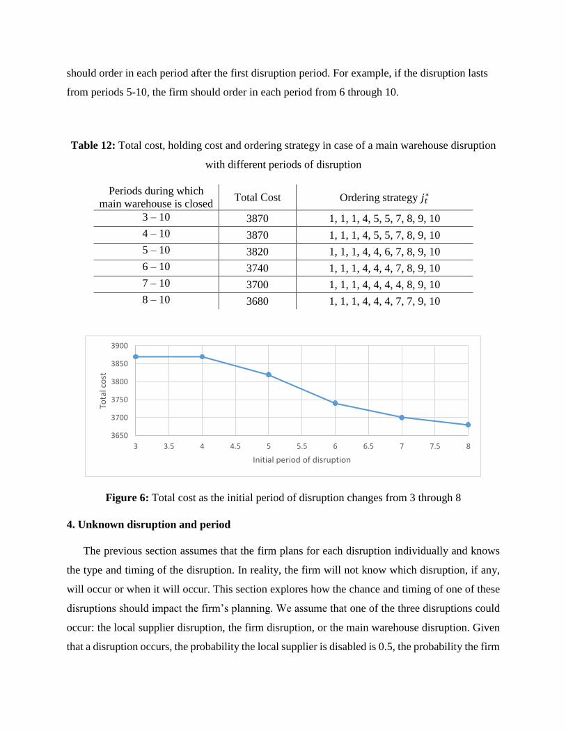
should order in each period after the first disruption period. For example, if the disruption lasts

from periods 5-10, the firm should order in each period from 6 through 10.

Table 12: Total cost, holding cost and ordering strategy in case of a main warehouse disruption

with different periods of disruption

Periods during which

main warehouse is closed Total Cost Ordering strategy 𝑗𝑡

∗

3 – 10 3870 1, 1, 1, 4, 5, 5, 7, 8, 9, 10

4 – 10 3870 1, 1, 1, 4, 5, 5, 7, 8, 9, 10

5 – 10 3820 1, 1, 1, 4, 4, 6, 7, 8, 9, 10

6 – 10 3740 1, 1, 1, 4, 4, 4, 7, 8, 9, 10

7 – 10 3700 1, 1, 1, 4, 4, 4, 4, 8, 9, 10

8 – 10 3680 1, 1, 1, 4, 4, 4, 7, 7, 9, 10

Figure 6: Total cost as the initial period of disruption changes from 3 through 8

4. Unknown disruption and period

The previous section assumes that the firm plans for each disruption individually and knows

the type and timing of the disruption. In reality, the firm will not know which disruption, if any,

will occur or when it will occur. This section explores how the chance and timing of one of these

disruptions should impact the firm’s planning. We assume that one of the three disruptions could

occur: the local supplier disruption, the firm disruption, or the main warehouse disruption. Given

that a disruption occurs, the probability the local supplier is disabled is 0.5, the probability the firm

3650

3700

3750

3800

3850

3900

3 3.5 4 4.5 5 5.5 6 6.5 7 7.5 8

Tota

l co

st

Initial period of disruption

is closed is 0.2, and the probability the main warehouse is closed is 0.3. We assume there is an

equal probability that the disruption will begin in period 3, 4, 5, 6, 7, or 8, equivalent to a 1/6

probability for each period. If the local supplier is disrupted, the firm can order from the alternate

supplier at a per-unit cost of 20. If the firm is disrupted, we assume the firm cannot satisfy any

demand while it is closed. If the main warehouse is disrupted, the firm can store inventory at the

alternate warehouses, but the holding cost increases to 5. We use the probabilities of disruption to

calculate the expected costs for each possible ordering strategy. The Wagner-Whitin algorithm is

deployed to find the order policy that minimizes the firm’s total expected cost. Since this is a

planning problem, the firm establishes an order before knowing whether a disruption occurs, which

disruption will occur, or when the disruption will occur.

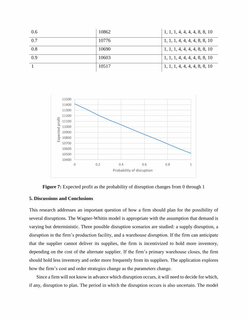
We vary the probability of a disruption between 0 and 1. The optimal ordering strategy for the

firm for different probabilities of disruptions is illustrated in Table 13. If the probability of a

disruption is less than 0.3, the firm should not change its ordering policy from the case without a

disruption. If the probability of a disruption is greater than or equal to 0.3, the firm should order in

periods 1, 4, 8, and 10. It becomes optimal to order in period 10 because the firm is incentivized

to plan for the firm being closed and for the main warehouse being closed. With such a large

probability of disruption, it becomes more likely that the firm will have a disrupted warehouse,

which increases its holding cost. Thus, it becomes more advantageous to hold less inventory and

order in period 10. (If the disruption disables the primary supplier, the firm’s cost of ordering does

not change based on whether it orders in period 8 or 10 because both periods require ordering from

the more expensive alternate supplier.) The expected profit decreases in a linear fashion as the

probability of a disruption increases as displayed in Figure 7.

Table 13: Probability of disruption and optimal planning for uncertain periods

Probability of disruption Expected profit Ordering strategy 𝑗𝑡∗

0 11420 1, 1, 1, 4, 4, 4, 4, 8, 8, 8

0.1 11318 1, 1, 1, 4, 4, 4, 4, 8, 8, 8

0.2 11215 1, 1, 1, 4, 4, 4, 4, 8, 8, 8

0.3 11121 1, 1, 1, 4, 4, 4, 4, 8, 8, 10

0.4 11035 1, 1, 1, 4, 4, 4, 4, 8, 8, 10

0.5 10949 1, 1, 1, 4, 4, 4, 4, 8, 8, 10

0.6 10862 1, 1, 1, 4, 4, 4, 4, 8, 8, 10

0.7 10776 1, 1, 1, 4, 4, 4, 4, 8, 8, 10

0.8 10690 1, 1, 1, 4, 4, 4, 4, 8, 8, 10

0.9 10603 1, 1, 1, 4, 4, 4, 4, 8, 8, 10

1 10517 1, 1, 1, 4, 4, 4, 4, 8, 8, 10

Figure 7: Expected profit as the probability of disruption changes from 0 through 1

5. Discussions and Conclusions

This research addresses an important question of how a firm should plan for the possibility of

several disruptions. The Wagner-Whitin model is appropriate with the assumption that demand is

varying but deterministic. Three possible disruption scenarios are studied: a supply disruption, a

disruption in the firm’s production facility, and a warehouse disruption. If the firm can anticipate

that the supplier cannot deliver its supplies, the firm is incentivized to hold more inventory,

depending on the cost of the alternate supplier. If the firm’s primary warehouse closes, the firm

should hold less inventory and order more frequently from its suppliers. The application explores

how the firm’s cost and order strategies change as the parameters change.

Since a firm will not know in advance which disruption occurs, it will need to decide for which,

if any, disruption to plan. The period in which the disruption occurs is also uncertain. The model

10400

10500

10600

10700

10800

10900

11000

11100

11200

11300

11400

11500

0 0.2 0.4 0.6 0.8 1

Exp

ecte

d p

rofi

t

Probability of disruption

applies probabilities to each disruption and the timing, and the firm chooses an order policy in

order to minimize its expected cost. Total profit is calculated based on the different probabilities

of disruptions. The firm’s ordering strategy may change as the probability of a disruption increases.

A firm who uses a manufacturing resource planning system that resembles the Wagner-Whitin

model could forecast possible disruptive events and explore if its ordering and production schedule

should change based on the possible disruptions. The incorporation of probability to account for

the uncertainty in the type and timing of disruptions allows a firm to understand how the likelihood

of a disruption should impact its planning and ordering strategy. For the illustrative example in

this chapter, the firm should slightly modify its ordering strategy as the probability of a disruption

occurs. Further research can seek to understand if generalized results can be derived from the

model about how the probability of disruption should impact a firm’s ordering strategy. Though

the Wagner-Whitin model generates an optimal planning horizon, it has some drawbacks. It has a

fixed setup cost and deterministic demand.

In the future, we plan to extend our methodology to more complex supply chains, which may

involve multiple suppliers. Future extensions can apply the algorithm to a real case study rather

than considering notional data. Having longer planning horizons and allowing the firm to respond

based on what disruption occurs may also impact the firm’s optimal planning.

6. References:

Adhyitya, A., Srinivasan, R., & Karimi, I. A. (2007). Heuristic rescheduling of crude oil operations

to manage abnormal supply chain events. American Institute of Chemical Engineers Journal,

53(2), 397-422.

Ambulkar, S., Blackhurst, J., & Grawe, S. (2015). Firm's resilience to supply chain disruptions:

Scale development and empirical examination. Journal of Operations Management, 33, 111-122.

Babich, V., Burnetas, A. N., & Ritchken, P. H. (2007). Competition and Diversification Effects in

Supply Chains with Supplier Default Risk. Manufacturing & Service Operations Management,

9(2), 123-146.

Bean, J.C., Birge, J.R.,Mittenthal, J. and Noon,C.E. (1991). Matchup scheduling with multiple

resources, release dates and disruptions. Operations Research, 39(3), 470–483.

Bode, C., & Wagner, S. M. (2015). Structural drivers of upstream supply chain complexity and

the frequency of supply chain disruptions. Journal of Operations Management, 36, 215-228.

Hendricks, K. B., Singhal, V. R., & Zhang, R. (2009). The effect of operational slack,

diversification, and vertical relatedness on the stock market reaction to supply chain disruptions.

Journal of Operations Management, 27(3), 233-246.

Hopp, W. J., Iravani, S. M. R., & Liu, Z. (2009). Strategic risk from supply chain disruptions.

Working paper. Department of Industrial Engineering and Management Sciences, Northwestern

University. Retrieved from

http://webuser.bus.umich.edu/whopp/working%20papers/Strategic%20Risk%20from%20Supply

%20Chain%20Disruptions.pdf

Hopp, W.J., & Spearman, M.L. (2008) Factory Physics, third edition, McGraw-Hill, Boston, MA.

Jeunet, J., & Jonard, N. (2000). Measuring the performance of lot-sizing techniques in uncertain

environments. International Journal of Production Economics, 64(1), 197-208.

Kazan, O., Nagi, R., & Rump, C. M. (2000). New lot-sizing formulations for less nervous

production schedules. Computers & Operations Research, 27(13), 1325-1345.

MacKenzie, C. A., Barker, K., & Grant, F. H. (2012). Evaluating the consequences of an inland

waterway port closure with a dynamic multiregional interdependence model. IEEE Transactions

on Systems, Man, and Cybernetics—Part A: Systems and Humans, 42(2), 359-370.

MacKenzie, C. A., Barker, K., & Santos, J. R. (2014). Modeling a severe supply chain disruption

and post-disaster decision making with application to the Japanese earthquake and tsunami. IIE

Transactions, 46(12), 1243-1260.

Natarajarathinam, M., Capar, I., & Narayanan, A. (2009). Managing supply chains in times of

crisis: a review of literature and insights. International Journal of Physical Distribution &

Logistics Management, 39(7), 535-573.

Papadakis, I. S. (2006). Financial performance of supply chains after disruptions: an event study.

Supply Chain Management: An International Journal, 11(1), 25-33.

Richter, K., & Weber, J. (2001). The reverse Wagner/Whitin model with variable manufacturing

and remanufacturing cost. International Journal of Production Economics, 71, 447-456.

Richter, K., & Sombrutzki, M. (2000). Remanufacturing planning for the reverse Wagner/Whitin

models. European Journal of Operational Research, 121(2), 304-315.

Sheffi, Y. (2005). The Resilient Enterprise: Overcoming Vulnerability for Competitive Advantage.

Cambridge: The MIT Press.

Schmitt, A. J., & Tomlin, B. (2012). Sourcing strategies to manage supply disruptions. In H.

Gurnani, A. Mehrotra, & S. Ray (Eds.), Supply Chain Disruptions: Theory and Practice of

Managing Risk (pp. 51-72). London: Springer.

Snyder, L. V., Atan, Z., Peng, P., Rong, Y., Schmitt, A. J., & Sinsoysal, B. (2016). OR/MS models

for supply chain disruptions: A review. IIE Transactions, 48(2), 89-109.

Snyder, L. V., Scaparra, M. P., Daskin, M. S., & Church, R. L. (2006). Planning for Disruptions

in Supply Chain Networks. Tutorials in Operations Research, 234-257.

Song, J.-S., & Zipkin, P. H. (1996). Inventory control with information about supply conditions.

Management Science, 42(10), 1409-1419.

Song, J.-S., & Zipkin, P. (2009). Inventories with multiple supply sources and networks of queues

with overflow bypasses. Management Science, 55(3), 362-372.

Tang, C. S. (2006). Perspectives in supply chain risk management. International Journal of

Production Economics, 103(2), 451-488.

Tomlin, B. (2006). On the value of mitigation and contingency strategies for managing supply

chain disruption risks. Management Science, 52(5), 639-657.

Vakharia, A. J., & Yenipazarli, A. (2008). Managing supply chain disruptions. Foundations and

Trends in Technology, Information and Operations Management, 2(4), 243-325.

Wagner, H. M. and T. M. Whitin (1958). Dynamic version of the economic lot size model.

Management Science, 9, 1, 89-96.

Xia, Y., Yang, M.-H., Golany, B., Gilbert, S. M., & Yu, G. (2004). Real-time disruption

management in a two-stage production and inventory system. IIE Transactions, 36, 111-125.

Xiao, T. and Qi, X. (2008) Price competition, cost and demand disruptions and coordination of a

supply chain with one manufacturer and two competing retailers. Omega, 36(5), 741–753.

Xiao, T. and Yu, G. (2006) Supply chain disruption management and evolutionarily stable

strategies of retailers in the quantity-setting duopoly situation with homogeneous goods. European

Journal of Operational Research, 173(2), 648–668.

Xiao, T., Yu, G., Sheng, Z. and Xia, Y. (2005) Coordination of a supply chain with one-

manufacturer and two-retailers under demand promotion and disruption management decisions.

Annals of Operations Research, 135(1), 87–109.