supplement for manifolds and difierential geometry · supplement for manifolds and difierential...
TRANSCRIPT
Supplement for Manifolds and Differential
Geometry
Jeffrey M. Lee
Department of Mathematics and Statistics, Texas Tech Uni-versity, Lubbock, Texas, 79409
Current address: Department of Mathematics and Statistics, Texas TechUniversity, Lubbock, Texas, 79409
E-mail address: [email protected]

Contents
§-1.1. Main Errata 1
Chapter 0. Background Material 5
§0.1. Sets and Maps 5
§0.2. Linear Algebra (under construction) 11
§0.3. General Topology (under construction) 15
§0.4. Shrinking Lemma 16
§0.5. Calculus on Euclidean coordinate spaces (underconstruction) 17
§0.6. Topological Vector Spaces 20
§0.7. Differential Calculus on Banach Spaces 25
§0.8. Naive Functional Calculus. 47
§0.9. Attaching Spaces and Quotient Topology 55
§0.10. Problem Set 57
Chapter 1. Chapter 1 Supplement 61
§1.1. Comments and Errata 61
§1.2. Rough Ideas I 61
§1.3. Pseudo-Groups and Models Spaces 68
§1.4. Sard’s Theorem 73
Chapter 2. Chapter 2 Supplement 77
§2.1. Comments and Errata 77
§2.2. Time Dependent Vector Fields 77
Chapter 5. Chapter 5 Supplement 81
v
vi Contents
§5.1. Comments and Errata 81§5.2. Matrix Commutator Bracket 81§5.3. Spinors and rotation 83§5.4. Lie Algebras 85§5.5. Geometry of figures in Euclidean space 98
Chapter 6. Chapter 6 Supplement 103§6.1. Comments and Errata 103§6.2. sections of the Mobius band 103§6.3. Etale space of a sheaf 104§6.4. Discussion on G bundle structure 105
Chapter 8. Chapter 8 Supplement 115§8.1. Comments and Errata 115§8.2. 2-Forms over a surface in Euclidean Space Examples. 115§8.3. Pseudo-Forms 117
Chapter 11. Chapter 11 Supplement 121§11.1. Comments and Errata 121§11.2. Singular Distributions 121
Chapter 12. Chapter 12 Supplement 127§12.1. Comments and Errata 127§12.2. More on Actions 127§12.3. Connections on a Principal bundle. 129§12.4. Horizontal Lifting 134
Chapter 13. Chapter 13 Supplement 137§13.1. Alternate proof of test case 137
Chapter 14. Complex Manifolds 139§14.1. Some complex linear algebra 139§14.2. Complex structure 142§14.3. Complex Tangent Structures 145§14.4. The holomorphic tangent map. 146§14.5. Dual spaces 147§14.6. The holomorphic inverse and implicit functions theorems. 148
Chapter 15. Symplectic Geometry 151§15.1. Symplectic Linear Algebra 151
Contents vii
§15.2. Canonical Form (Linear case) 153§15.3. Symplectic manifolds 153§15.4. Complex Structure and Kahler Manifolds 155§15.5. Symplectic musical isomorphisms 158§15.6. Darboux’s Theorem 159§15.7. Poisson Brackets and Hamiltonian vector fields 160§15.8. Configuration space and Phase space 163§15.9. Transfer of symplectic structure to the Tangent bundle 165§15.10. Coadjoint Orbits 167§15.11. The Rigid Body 168§15.12. The momentum map and Hamiltonian actions 170
Chapter 16. Poisson Geometry 173§16.1. Poisson Manifolds 173
Chapter 17. Geometries 177§17.1. Group Actions, Symmetry and Invariance 183§17.2. Some Klein Geometries 187
Bibliography 209
Index 213

-1.1. Main Errata 1
-1.1. Main Errata
Chapter 1
(1) Page 3. Near the end of the page “...we have a second derivativeD2f(a) : Rn → L(Rn,Rm)” should read
“...we have a second derivative D2f(a) : Rn → L(Rn, L(Rn,Rm))”
(2) . Page 4. The is a missing exponent of 2 in the partial derivativesin the display at the top of the page. It should (of course) read as
ui =∑
j,k
∂2f i
∂xj∂xk(a)vjwk.
(3) Page 19, forth line from the top at the beginning of Notation 1.44:
(x1, . . . , xn+1) ∈ Rn+1
should be changed to
(x1, . . . , xn+1) ∈ Rn+1\0(4) Page 23. 6th line from the top. The expression y f x|−1
α shouldbe changed to yβ f xα|−1
U
Chapter 2
(1) Page 61. The curve defined in the 6th line from the bottom of thepage is missing a t and should read as follows:
ci(t) := x−1(x(p) + tei),
(2) Page 68. In Definition 2.19: “...so a tangent vector in TqM” shouldread “...so a tangent vector in TqN”.
(3) Page 73. At the end of the second display, (M2, p) should bechanged to (M2, q).
(4) Page 109. In the proof of Theorem 2.113, the first display shouldread
X1(p), . . . , Xk(p),∂
∂yk+1
∣∣∣∣p
, . . . ,∂
∂yn
∣∣∣∣p
(The initially introduced coordinates are y1, ...., yn.)
(5) On Page 115, in the second set of displayed equations there is both aspurious q and a spurious p (although, the action of the derivationsin question are indeed happening at the respective points: The
2 Contents
display should read as follows:
(φ∗df)|p v = df |q (Tpφ · v)
= ((Tpφ · v) f)
= v (f φ) = d(φ∗f)|p v.
(6) Page 124. Problem (18). The second to last line of part (b) weshould find T0R
n = ∆∞ ∼=(m∞/m2∞
)∗.Chapter 3
(1) Page 167, Equation 4.3.Equation 4.3 is missing a square root. It should read
L(c) =∫ b
a
( n−1∑
i,j=1
gij(c(t))dci
dt
dcj
dt
)1/2
dt,
where ci(t) := ui c.
(2) The last displayed set of equations on page 175 is missing twosquare roots in the integrands and should read as follows:
L(γ) =∫ b
a‖γ(t)‖ dt =
∫ b
a
⟨∑ dui
dt
∂x∂ui
,∑ duj
dt
∂x∂uj
⟩1/2
dt
=∫ b
a
(n−1∑
i,j
gij(u(t))dui
dt
duj
dt
)1/2
dt,
Chapter 5
(1) Page 212. In the first displayed equation in the proof of Theorem5.7.2, the time derivative should be taken at an arbitrary time tand so d
dt
∣∣t=0
c(t) should be changed to ddt c(t).
(2) Page 218. The latter part of the third sentence in the proof ofTheorem 5.81 on page 218 should read ”is a relatively closed set inU”.
Chapter 9
(1) Page 395. All integrations in the first set of displayed equationsshould be over the entire space Rn. (In an earlier version I hadput the support in the left half space but after changing my mindI forgot to modify these integrals.)
(2) Page 395. In ”Case 2” right before the line the begins “If j = 1”,the variable u1 ranges from −∞ to 0 and so “=
∫Rn−1” should be
replaced by “=∫Rn−1
u1≤0
”.
-1.1. Main Errata 3
(3) Page 395. In ”Case 2” right after the line the begins “If j = 1”,the displayed equation should read
∫
Rnu1≤0
dω1 =∫
Rn−1
(∫ 0
−∞
∂f
∂u1du1
)du2 · · · dun
(4) Page 396. In the first line of the second set of displayed equationsa Uα need to be changed to M . Also, we use the easily verified factthat
∫M ω =
∫U ω when the support of ω is contained in an open
set U . (We apply this to the ραω in the proof.) The display shouldread:∫
Mdω =
∫
M
∑α
d(ραω) =∑α
∫
Uα
d(ραω)
=∑α
∫
xα(Uα)(x−1
α )∗d(ραω) =∑α
∫
xα(Uα)d((x−1
α )∗ραω)
=∑α
∫
∂xα(Uα)((x−1
α )∗ραω) =∑α
∫
∂Uα
ραω =∫
∂Mω,
(5) Page 396-397. Starting at the bottom of 396 and continuing onto397, all references to the interval (−π, π) should obviously be changedto (0, π). The integrals at the top of page 397 should be changedaccordingly.
(6) Page 399. The last line before the final display should read ”where(ρXk)i := d(ρXk)(Ei) for all k, i.”
Chapter 10
(1) On page 444 immediately before Definition 10.3, the following shouldbe inserted: Recall that if a sequence of module homomorphisms,
· · · → Ak−1fk→ Ak fk+1→ Ak+1 → · · · has the property that Ker(fk+1) =
Im(fk), then we say that the sequence is exact at Ak and the se-quence is said to be exact if it is exact at Ak for all k (or all k suchthat the kernel an image exist).
(2) Page 444. In the middle of the page, the sentence that definesa chain map should state that the map is linear. Indeed, in thissection it is likely that all maps between modules or vector spacesare linear by default.
(3) Page 444. The last line before definition 10.5 should read “x ∈Zk(A)”. The following should be added: Note that if x − x′ = dythen f(x)− f(x′) = f(dy) = d(f(y) so that f(x) ∼ f(x′).
(4) Page 451. In the second and third lines of the first display of ”CaseI”, the factor (−1)k should be omitted (in both lines). This factordoes appear in the forth line.
4 Contents
(5) Page 451. In the second to last display there is a spurious “*”.Replace (f sa π∗) π∗α by (f sa π) π∗α.
Appendicies
(1) Page 639, Definition A.4,“A morphism that is both a monomorphism and an epimor-
phism is called an isomorphism.”should be changed to“A morphism that is both a monomorphism and an epimorphismis called a bimorphism. A morphism is called an isomorphismif it has both a right and left inverse.”
(2) Page 648. In the constant rank theorem a q needs to be changedto a 0. We should read “...there are local diffeomorphisms g1 :(Rn, p) → (Rn, 0)”.
Chapter 0
Background Material
0.1. Sets and Maps
Any reader who already knows the meaning of such words as domain, codomain,surjective, injective, Cartesian product, and equivalence relation, should justskip this section to avoid boredom.
According to G. Cantor, one of the founders of set theory, a set is a col-lection of objects, real or abstract, taken as a whole or group. The objectsmust be clear and distinct to the intellect. If one considers the set of allducks on a specific person’s farm then this seems clear enough as long as thenotion of a duck is well defined. But is it? When one thinks about the setof all ducks that ever lived, then things get fuzzy (think about evolutionarytheory). Clearly there are philosophical issues with how we define and thinkabout various objects, things, types, kinds, ideas and collections. In math-ematics, we deal with seemingly more precise, albeit abstract, notions andobjects such as integers, letters in some alphabet or a set of such things (ora set of sets of such things!). We will not enter at all into questions aboutthe clarity or ontological status of such mathematical objects nor shall wediscuss “proper classes”. Suffice it to say that there are monsters in thoseseas.
Each object or individual in a set is called an element or a memberof the set. The number 2 is an element of the set of all integers-we say itbelongs to the set. Sets are equal if they have the same members. Weoften use curly brackets to specify a set. The letter a is a member of theset a, B, x, 6. We use the symbol ∈ to denote membership; a ∈ A means“a is a member of the set A”. We read it in various ways such as “a is aelement of A” or “a in A”. Thus, x ∈ a,B, x, 6 and if we denote the set of
5
6 0. Background Material
natural numbers by N then 42 ∈ N and 3 ∈ N etc. We include in our naivetheory of sets a unique set called the empty set which has no members atall. It is denoted by ∅ or by . Besides just listing the members of a set wemake use of notation such as x ∈ N : x is prime which means the set ofall natural numbers with the property of being a prime numbers. Anotherexample; a : a ∈ N and a < 7. This is the same set as 1, 2, 3, 4, 5, 6.
If every member of a set A is also a member of a set B then we saythat A is a subset of B and write this as A ⊂ B or B ⊃ A. Thus ifa ∈ A =⇒ b ∈ A. (The symbol “=⇒” means “implies”). The empty set is asubset of any set we may always write ∅ ⊂ A for any A. Also, A ⊂ A forany set A. It is easy to see that if A ⊂ B and B ⊂ A then A and B havethe same members–they are the same set differently named. In this case wewrite A = B. If A ⊂ B but A 6= B then we say that A is a proper subsetof B and write A $ B.
The union of two sets A and B is defined to be the set of all elements thatare members of either A or B (or both). The union is denoted A∪B. Thusx ∈ A∪B if and only if x ∈ A or x ∈ B. Notice that here by “x ∈ A or x ∈ B”we mean to allow the possibility that x might be a member of both A and B.The intersection of A and B the set of elements belonging to both A andB. We denote this by A∩B. For example, 6, π,−1, 42, −1∩N = 6, 42(Implicitly we assume that no two elements of a set given as a list are equalunless they are denoted by the same symbol. For example, in 6, a, B, x, 42,context implies that a 6= 42.) If A∩B = ∅ then A and B have no elementsin common and we call them disjoint.
There are the following algebraic laws: If A, B, and C are sets then
(1) A ∩B = B ∩A and A ∪B = B ∪A (Commutativity),
(2) (A ∪B)∪C = A∪ (B ∪ C) and (A ∩B)∩C = A∩ (B ∩ C) (Asso-ciativity),
(3) A ∪ (B ∩ C) = (A ∪B) ∩ (A ∪ C) and A ∩ (B ∪ C) = (A ∩B) ∪(A ∩ C) (Distributivity). It follows that we also have
(4) A ∪ (A ∩B) = A and A ∩ (A ∪B) = A
We can take A∪B ∪C to mean (A ∪B)∪C. In fact, if A1, · · · , An are setsthan we can inductively make sense out of the union A1 ∪A2 ∪ · · · ∪An andintersection A1 ∩A2 ∩ · · · ∩An.
If A and B are sets then A\B denotes that set of all elements of A thatare not also elements of B. The notation A − B is also used and is calledthe difference. When considering subsets of a fix set X determined by thecontext of the discussion we can denote X\A as Ac and refer to Ac as thecomplement of A (in X). For example, if A is a subset of the set of real
0.1. Sets and Maps 7
numbers (denoted R) then Ac = R\A. It is easy to see that if A ⊂ B thenBc ⊂ Ac. We have de Morgan’s laws:
(1) (A ∪B)c = Ac ∩Bc
(2) (A ∩B)c = Ac ∪Bc
A family of sets is just a set whose members are sets. For example,for a fixed set X we have the family P(X) of all subsets of X. The familyP(X) is called the power set of X. Note that ∅ ∈ P(X). If F is somefamily of sets then we can consider the union or intersection of all the setsin F .
⋃A∈FA := x : x ∈ A for some A ∈ F⋂A∈FA := x : x ∈ A for every A ∈ F
It is often convenient to consider indexed families of sets. For example,if A1, A2, and A3 are sets then we have a family A1, A2, A3 indexed bythe index set 1, 2, 3. The family of sets may have an infinite number ofmembers and we can use an infinite index set. If I is an index set (possiblyuncountably infinite) then a family F indexed by I has as members setswhich are each denoted Ai for some i ∈ I and some fixed letter A. Fornotation we use
F = Ai : i ∈ I or Aii∈I .
We can then write unions and intersections as ∪i∈IAi and ∩i∈IAi. De Mor-gan’s laws become
(⋃i∈IAi
)c =⋂
i∈IAci ,(⋂
i∈IAi
)c =⋃
i∈IAci .
A partition of a set X is a family of subsets of X, say Aii∈I such thatAi ∩Aj = ∅ when ever i 6= j and such that X =
⋃i∈IAi.
An ordered pair with first element a and second element b is denoted(a, b). To make this notion more precise one could take (a, b) to be the seta, a, b. Since the notion of an ordered pair is so intuitive it is seldomnecessary to resort to thinking explicitly of a, a, b. Given two sets A andB, the Cartesian product of A and B is the set of order pairs (a, b) wherea ∈ A and b ∈ B. We denote the Cartesian product of A and B by A× B.We can also consider ordered n-tuples such as (a1, ..., an). For a list of setsA1, A2, . . . , Ak we define the n-fold Cartesian product:
A1 ×A2 × · · · ×An := (a1, ..., an) : ai ∈ Ai.If A = A1 = A2 = · · · = An then we denote A1 ×A2 × · · · ×An by An. Forany set X the diagonal subset ∆X of X ×X is defined by ∆X := (a, b) ∈X ×X : a = b = (a, a) : a ∈ X.
8 0. Background Material
Example 0.1. If R denotes the set of real numbers then, for a given positiveinteger n, Rn denotes the set of n-tuples of real numbers. This set has a lotof structure as we shall see.
One of the most important notions in all of mathematics is the notionof a “relation”. A relation from a set A to a set B is simply a subset ofA × B. A relation from A to A is just called a relation on A. If R is arelation from A to B then we often write aR b instead of (a, b) ∈ R. Wesingle out two important types of relations:
Definition 0.2. An equivalence relation on a set X is a relation on X,usual denoted by the symbol ∼, such that (i) x ∼ x for all x ∈ X, (ii) x ∼ yif and only if y ∼ x, (iii) if x ∼ y and y ∼ z then x ∼ z. For each a ∈ X theset of all x such that x ∼ a is called the equivalence class of a (often denotedby [a]). The set of all equivalence classes form a partition of X. The set ofequivalence classes if often denoted by X/∼.
Conversely, it is easy to see that if Aii∈I is a partition of X then wemy defined a corresponding equivalence relation by declaring x ∼ y if andonly if x and y belong to the same Ai.
For example, ordinary equality is an equivalence relation on the set ofnatural numbers. Let Z denote the set of integers. Then equality moduloa fixed integer p defines and equivalence relation on Z where n ∼ m iff1
n − m = kp for some k ∈ Z. In this case the set of equivalence classes isdenoted Zp or Z/pZ.
Definition 0.3. A partial ordering on a set X (assumed nonempty) isa relation denoted by, say ¹, that satisfies (i) x ¹ x for all x ∈ X, (ii) ifx ¹ y and y ¹ x then x = y , and (iii) if x ¹ y and y ¹ z then x ¹ z. Wesay that X is partially ordered by ¹. If a partial ordering also has theproperty that for every x, y ∈ X we have either x ¹ y or y ¹ x then we callthe relation a total ordering or (linear ordering). In this case, we say thatX is totally ordered by ¹.
Example 0.4. The set of real numbers is totally ordered by the familiarnotion of less than; ≤.
Example 0.5. The power set P(X) is partially ordered by set inclusion ⊂(also denoted ⊆).
If X is partially ordered by ¹ then an element x is called a maximalelement if x ¹ y implies x = y. A minimal element is defined similarly.
1“iff” means ”if and only if”.
0.1. Sets and Maps 9
Maximal elements might not be unique or even exist at all. If the relation isa total ordering then a maximal (or minimal) element, if it exists, is unique.
A rule that assigns to each element of a set A an element of a set B iscalled a map, mapping, or function from A to B. If the map is denoted byf , then f(a) denotes the element of B that f assigns to a. If is referred toas the image of the element a. As the notation implies, it is not allowedthat f assign to an element a ∈ A two different elements of B. The set A iscalled the domain of f and B is called the codomain of f . The domain ancodomain must be specified and are part of the definition. The prescriptionf(x) = x2 does not specify a map or function until we specify the domain. Ifwe have a function f from A to B we indicate this by writing f : A → B orA
f→ B. If a is mapped to f(a) indicate this also by a 7→ f(a). This notationcan be used to define a function; we might say something like “consider themap f : Z→ N defined by n 7→ n2 + 1.” The symbol “7→” is read as “mapsto” or “is mapped to”.
It is desirable to have a definition of map that appeals directly to thenotion of a set. To do this we may define a function f from A to B to be arelation f ⊂ A×B from A to B such that if (a, b1) ∈ f and (a, b2) ∈ f thenb1 = b2.
Example 0.6. The relation R ⊂ R × R defined by R := (a, b) ∈ R × R :a2 +b2 = 1 is not a map. However, the relation (a, b) ∈ R×R : a2−b = 1is a map; namely the map R → R defined, as a rule, by a 7→ a2 − 1 for alla ∈ R.
Definition 0.7. (1) A map f : A → B is said to be surjective (or “onto”)if for every b ∈ B there is at least one ma∈ A such that f(a) = b. Such amap is called a surjection and we say that f maps A onto B.(2) A map f : A → B is said to be injective (or “one to one”) if wheneverf(a1) = f(a2) then a1 = a2. We call such a map an injection.
Example 0.8. The map f : R → R3 given by f : t 7→ (cos t, sin t, t) isinjective but not surjective. Let S2 := (x, y) ∈ R2 : x2 + y2 = 1 denotethe unit circle in R2. The map f : R → S2 given by t 7→ (cos t, sin t) issurjective but not injective. Note that specifying the codomain is essential;the map f : R → R2 also given by the formula t 7→ (cos t, sin t) is notsurjective.
The are some special maps to consider. For any set A we have theidentity map idA : A → A such idA(a) = a for all a ∈ A. If A ⊂ X then themap ıA,X from A to X given by ıA,X(a) = a is called the inclusion mapfrom A into X. Notice that idA and ıA,X are different maps since they havedifferent codomains. We shall usually abbreviate ıA,X to ı and suggestivelywrite ı : A → X instead of ı : A → X.
10 0. Background Material
When we have a map f : A → B there is are tow induced maps on powersets. For S ⊂ A let use define f(S) := b ∈ B : b = f(s) for some s ∈ S.Then reusing the symbol f we obtain a map f : P (A) → P (B) given byS 7→ f(S). We call f(S) the image of S under f . We have the followingproperties
(1) If S1, S2 ⊂ A then f (S1 ∪ S2) = f (S1) ∪ f (S2),
(2) If S1, S2 ⊂ A then f (S1 ∩ S2) ⊂ f (S1) ∩ f (S2).
A second map is induced on power sets f−1 : P (B) → P (A). Notice theorder reversal. Here the definition of f−1(E) for E ⊂ B is f−1(E) := a ∈A : f(a) ∈ B. This time the properties are even nicer:
(1) If E1, E2 ⊂ B then f−1 (E1 ∪ E2) = f−1 (E1) ∪ f−1 (E2)
(2) If E1, E2 ⊂ B then f−1 (E1 ∩ E2) = f−1 (E1)∩f−1 (E2) (equality!)
(3) f−1(Ec) =(f−1(E)
)c
In fact, these ideas work in more generality. For example, if Eii∈I ⊂ P (B)then f−1
(⋃i∈IEi
)=
⋃i∈If
−1 (Ei) and similarly for intersection.Now suppose that we have a map f : A → B and another map g : B → C
then we can form the composite map g f : A → C (or composition)by (g f) (a) = g (f(a)) for a ∈ A. Notice that we have been carefullyassumed that the codomain of f is also the domain of g. But in many areasof mathematics this can be relaxed. For example, if we have f : A → B andg : X → C where B ⊂ X then we can define g f by the same prescriptionas before. In some fields (such as algebraic topology) this is dangerous andone would have to use an inclusion map g ıB,X f . In some cases we can beeven more relaxed and compose maps f : A → B and g : X → C by lettingthe domain of g f be a ∈ A : f(a) ∈ X assuming this set is not empty.
If f : A → B is a given map and S ⊂ A then we obtain a map f |S :S → B by the simple rule f |S (a) = f(a) for a ∈ S. The map f |S is calledthe restriction of f to S. It is quite possible that f |S is injective even if fis not (think about f(x) = x2 restricted to x > 0).Definition 0.9. A map f : A → B is said to be bijective and referred toas a bijection if it is both a surjection and an injection. In this case wesay that f is a one to one correspondence between A and B. If f is abijection then we have the inverse map f−1 : B → A defined by stipulatingthat f−1(b) is equal to the unique ma∈ A such that f(a) = b. In this casewe have f f−1 = idB and f−1 f = idA.
It is sometimes convenient and harmless to relax our thinking about f−1.If f : A → B is injective but not surjective then there is a bijective map inthe offing. This map has codomain f(A) and otherwise agrees with f . It is
0.2. Linear Algebra (under construction) 11
just f considered as a map onto f(A). What shall we call this map? If weare careful to explain ourselves we can use the same letter f and then wehave an inverse map f−1 : f(A) → A. We say that the injective map f is abijection onto its image f(A).
If a set contains only a finite number of elements then that number iscalled the cardinality of the set. If the set is infinite we must be moreclever. If there exists some injective map from A to B we say that thecardinality of A is less than the cardinality of B and write |A| ≤ |B|. Ifthere exists some surjective map from A to B we say that the cardinality ofA is greater than the cardinality of B and write |A| ≥ |B|. If there exists abijection then we say the sets have the same cardinality and write |A| = |B|.The Schroder-Bernstein theorem states that if |A| ≤ |B| and |A| ≥ |B| then|A| = |B|. This is not obvious. If there exist an injection but no bijectionthen we write |A| < |B|.Definition 0.10. If there exists a bijection from A to the set of naturalnumbers N then we say that A a countably infinite set. If A is either afinite set or countably infinite set we say it is a countable set. If |N| < |A|then we say that A is uncountable.
Example 0.11. The set of rational numbers, Q is well known to be count-ably infinite while the set of real numbers is uncountable (Cantor’s diagonalargument).
0.2. Linear Algebra (under construction)
We will defined vector space below but since every vector space has a socalled base field, we should first list the axioms of a field. Map from A×A toanother set (often A) is sometimes called an operation. When the operationis denoted by a symbol such as + then we write a + b in place of +(a, b).The use of this symbol means we will refer to the operation as addition.Sometimes the symbol for the operation is something like · or ¯ in which casewe would write a · b and call it multiplication. In this case we will actuallydenote the operation simply by juxtaposition just as we do for multiplicationof real or complex numbers. Truth be told, the main examples of fieldsare the real numbers or complex numbers with the familiar operations ofaddition and multiplication. The reader should keep these in mind whenreading the following definition but also remember that the ideas are purelyabstract and many examples exist where the meaning of + and · is somethingunfamiliar.
Definition 0.12. A set F together with an operation + : F×F→ F and anoperation · also mapping F× F→ F is called a field is the following axiomsare satisfied.
12 0. Background Material
F1. r + s = s + r. for all r, s ∈ FF2. (r + s) + t = r + (s + t). for all r, s, t ∈ FF3. There exist a unique element 0 ∈ F such that r + 0 = r for all
r ∈ F.F4. For every r ∈ F there exists a unique element −r such that r +
(−r) = 0.
F5. r · s = s · r for all r, s ∈ F.F6. (r · s) · t = r · (s · t)F7. There exist a unique element 1 ∈ F, such that 1 6= 0 and such that
1 · r = r for all r ∈ F.F8. For every r ∈ F with r 6= 0 there is a unique element r−1 such that
r · r−1 = 1.
F9. r · (s + t) = r · s + r · t for all r, s, t ∈ F.
Most of the time we will write rs in place of r · s. We may use someother symbols such as ⊕ and ¯ in order to distinguish from more familiaroperations. Also, we see that a field is really a triple (F,+, ·) but we followthe common practice of referring to the field by referring to the set so we willdenote the field by F and speak of elements of the field and so on. The fieldof real numbers is denoted R and the field of complex numbers is denoted C.We use F to denote some unspecified field but we will almost always haveR or C in mind. Another common field is the the set Q of rational numberswith the usual operations.
Example 0.13. Let p be some prime number. Consider the set Fp =0, 1, 2, ..., p − 1. Define an addition ⊕ on Fp by the following rule. Ifx, y ∈Fp then let x ⊕ y be the unique z ∈ Fp such that x + y = z + kp forsome integer k. Now define a multiplication by x ¯ y = w where w is theunique element of Fp such that xy = w + kp for some integer k. Using thefact that p is prime it is possible to show that (Fp,⊕,¯) is a (finite) field.
Consider the following sets; Rn, the set C([0, 1]) of continuous functionsdefined on the closed interval [0, 1], the set of n ×m real matrices, the setof directed line segments emanating from a fixed origin in Euclidean space.What do all of these sets have in common? Well, one thing is that in eachcase there is a natural way to add elements of the set and was way to “scale”or multiply elements by real numbers. Each is natural a real vector space.Similarly, Cn and complex n × m matrices and many other examples arecomplex vectors spaces. For any field F we define an F-vector space or avector space over F. The field in question is called the field of scalars forthe vector space.
0.2. Linear Algebra (under construction) 13
Definition 0.14. A vector space over a field F is a set V together with anaddition operation V × V → V written (v, w) 7→ v + w and an operationof scaling F × V → V written simply (r, v) 7→ rv such that the followingaxioms hold:
V1. v + w = w + v for all v, w ∈ V .V2. (u + v) + w = u + (v + w) for all u, v, w ∈ V .V3. The exist a unique member of V denoted 0 such that v +0 = v for
all v ∈ V .V4. For each v ∈ V there is a unique element−v such that v+(−v) = 0.V5. (rs) v = r (sv) for all r, s ∈ F and all v ∈ V .V6. r (v + w) = rv + rw for all v, w ∈ V and r ∈ F.V7. (r + s) v = rv + sv for all r, s ∈ F and all v ∈ V .V8. 1v = v for all v ∈ V .
Notice that in axiom V7 the + on the left is the addition in F while thaton the right is addition in V . These are separate operations. Also, in axiomV4 the −v is not meant to denote −1v. However, it can be shown from theaxioms that it is indeed true that −1v = −v.
Examples Fn.SubspacesLinear combinations, Span, span(A) for A ⊂ V .Linear independenceBasis, dimensionChange of basisTwo bases E = (e1, . . . , en) and E = (e1, . . . , en) are related by a non-
sigular matrix C according to ei =∑n
j=1 Cji ej . In this case we have v =∑n
i=1 viei =∑n
j=1 vj ej . On the other hand,
n∑
j=1
vj ej = v =n∑
i=1
viei =n∑
i=1
vi
n∑
j=1
Cji ej
=n∑
j=1
(n∑
i=1
Cji v
i
)ej
from which we deduce that
vj =n∑
i=1
Cji v
i.
L : V → W
14 0. Background Material
Lej =m∑
i=1
Aijfi
Lv = L
n∑
j=1
vjej =n∑
j=1
vjLej =n∑
j=1
vj
(m∑
i=1
Aijfi
)
=m∑
i=1
n∑
j=1
Aijv
j
fi
From which we conclude that if Lv = w =∑
wifi then
wi =n∑
j=1
Aijv
j
Consider another basis fi and suppose fi =∑m
j=1 Dji fj . Of course, wi =∑n
j=1 Aij v
j where Lej =∑m
i=1 Aij fi and w =
∑wifi.
Lej =∑m
i=1 Aijfi and
Lej =m∑
i=1
Aijfi =
m∑
i=1
Aij
(m∑
k=1
Dki fk
)
=m∑
k=1
(m∑
i=1
Dki Ai
j
)fk
But also
Lej = Ln∑
r=1
Crj er =
n∑
r=1
Crj Ler
=n∑
r=1
Crj
(m∑
k=1
Akr fk
)=
m∑
k=1
(n∑
r=1
AkrC
rj
)fk
and som∑
i=1
Dki Ai
j =n∑
r=1
AkrC
rj
n∑
j=1
m∑
i=1
Dki Ai
j
(C−1
)j
s=
n∑
j=1
n∑
r=1
AkrC
rj
(C−1
)j
s
n∑
j=1
m∑
i=1
Dki Ai
j
(C−1
)j
s=
n∑
r=1
Akrδ
rs = Ak
s
Aks =
n∑
j=1
m∑
i=1
Dki Ai
j
(C−1
)j
s
0.3. General Topology (under construction) 15
and so
Aks =
m∑
i=1
Dki Ai
j
(C−1
)j
s
Linear maps– kernel, image rank, rank-nullity theorem. Nonsingular,isomorphism, inverse
Vector spaces of linear mapsGroup GL(V )ExamplesMatrix representatives, change of basis, similarityGL(n,F)Dual Spaces, dual basisdual mapcontragedientmultilinear mapscomponents, change of basistensor productInner product spaces, Indefinite Scalar Product spacesO(V ), O(n), U(n)Normed vector spaces, continuityCanonical Forms
0.3. General Topology (under construction)
metricmetric spacenormed vector spaceEuclidean spacetopology (System of Open sets)Neighborhood systemopen setneighborhoodclosed setclosureaherent pointinterior pointdiscrete topology
16 0. Background Material
metric topologybases and subbasescontinuous map (and compositions etc.)open maphomeomorphismweaker topology stronger topologysubspacerelatively open relatively closedrelative topologyproduct spaceproduct topologyaccumulation pointscountability axiomsseparation axiomscoveringslocally finitepoint finitecompactness (finite intersection property)image of a compact spacerelatively compactparacompactness
0.4. Shrinking Lemma
Theorem 0.15. Let X be a normal topological space and suppose thatUαα∈A is a point finite open cover of X. Then there exists an open coverVαα∈A of X such that V α ⊂ Uα for all α ∈ A.
second proof. We use Zorn’s lemma (see [Dug]). Let T denote the topol-ogy and let Φ be the family of all functions ϕ : A → T such thati) either ϕ(α) = Uα or ϕ(α) = Vα for some open Vα with V α ⊂ Uα
ii) ϕ(α) is an open cover of X.We put a partial ordering on the family Φ by interpreting ϕ1 ≺ ϕ2 to meanthat ϕ1(α) = ϕ2(α) whenever ϕ1(α) = Vα (with V α ⊂ Uα). Now let Ψ be atotally order subset of Φ and set
ψ∗(α) =⋂
ψ∈Ψ
ψ(α)
0.5. Calculus on Euclidean coordinate spaces (underconstruction) 17
Now since Ψ is totally ordered we have either ψ1 ≺ ψ2 or ψ2 ≺ ψ1. We nowwhich to show that for a fixed α the set ψ(α) : ψ ∈ Ψ has no more than twomembers. In particular, ψ∗(α) is open for all α. Suppose that ψ1(α), ψ2(α)and ψ3(α) are distinct and suppose that ψ1 ≺ ψ2 ≺ ψ3 without loss. Ifψ1(α) = Vα with V α ⊂ Uα then we must have ψ2(α) = ψ3(α) = Vα by defi-nition of the ordering but this contradicts the assumption that ψ1(α), ψ2(α)and ψ3(α) are distinct. Thus ψ1(α) = Uα. Now if ψ2(α) = Vα for withV α ⊂ Uα then ψ3 (α) = Vα also a contradiction. The only possibility left isthat we must have both ψ1(α) = Uα and ψ2(α) = Uα again a contradiction.Now the fact that ψ(α) : ψ ∈ Ψ has no more than two members for everyα means that ψ∗ satisfies condition (i) above. We next show that ψ∗ alsosatisfies condition (ii) so that ψ∗ ∈ Φ. Let p ∈ X be arbitrary. We havep ∈ ψ(α0) for some α0.By the locally finite hypothesis, there is a finite set Uα1 , ...., Uαn ⊂ Uαα∈A
which consists of exactly the members of Uαα∈A that contain p. Nowψ∗(αi) must be Uαi or Vαi . Since p is certainly contained in Uαi we mayas well assume the worst case where ψ∗(αi) = Vαi for all i. There must beψi ∈ Ψ such that ψ∗(αi) = ψi(αi) = Vαi . By renumbering if needed, we mayassume that
ψ1 ≺ · · · ≺ ψn
Now since ψn is a cover we know that x is in the union of the set in thefamily
ψn(α1), ...., ψn(αn) ∪ ψn(α)α∈A\α1,....αnbut it must be that x ∈ ψn(αi) for some i. Since ψi ¹ ψn we have x ∈ψi(αi) = ψ∗(αi). Thus since x was arbitrary we see that ψ∗(α)α∈A is acover and hence ψ∗ ∈ Ψ. By construction, ψ∗ = supΨ and so by Zorn’slemma Φ has a maximal element ϕmax. We now show that ϕmax(α) =V α ⊂ Uα for every α. Suppose by way of contradiction that ϕmax(β) = Uβ
for some β. Let Xβ = X − ∪α 6=βϕmax(α). Since ϕmax(α)α∈A is a coverwe see that Xβ is a closed subset of Uβ. Applying normality we obtainXβ ⊂ Vβ ⊂ V β ⊂ Uβ. Now if we define ϕβ : A → T by
ϕβ(α) :=
ϕmax(α) for α 6= βVβ for α = β
then we obtain an element of Φ which contradicts the maximality of ϕmax.¤
0.5. Calculus on Euclidean coordinate spaces(underconstruction)
0.5.1. Review of Basic facts about Euclidean spaces. For each posi-tive integer d, let Rd be the set of all d-tuples of real numbers. This means
18 0. Background Material
that Rd := R× · · ·×d times
R. Elements of Rd are denoted by notation such as
x := (x1, . . . , xd). Thus, in this context, xi is the i-th component of x andnot the i-th power of a number x. In the context of matrix algebra weinterpret x = (x1, . . . , xd) as a column matrix
x =
x1
...xd
Whenever possible we write d-tuples horizontally. We use both superscriptand subscripts since this is so common in differential geometry. This takessome getting used to but it ultimately has a big payoff. The set Rd isendowed with the familiar real vector space structure given by
x + y = (x1, . . . , xd) + (y1, . . . , yd) = (x1 + y1, . . . , xd + yd)
ax = (ax1, . . . , axd) for a ∈ R.
We denote (0, ..., 0) as simply 0. Recall that if v1, ..., vk ⊂ Rd then we saythat a vector x is a linear combination of v1, ..., vk if x = c1v1 + · · · + ckvk
for some real numbers c1, ..., ck. In this case we say that x is in the span ofv1, ..., vk or that it is a linear combination the elements v1, ..., vk. Also,a set of vectors, say v1, ..., vk ⊂ Rd, is said to be linearly dependentif for some j, with 1 ≤ j ≤ d we have that vj is a linear combination ofthe remaining elements of the set. If v1, ..., vk is not linearly dependentthen we say it is linearly independent. Informally, we can refer directlyto the elements rather than the set; we say things like “v1, ..., vk are linearlyindependent”. An ordered set of elements of Rd, say (v1, ..., vd), is said tobe a basis for Rd if it is a linearly independent set and every member of Rd
is in the span of this set. In this case each element x ∈ Rd can be writtenas a linear combination x = c1v1 + · · ·+ cdvd and the ci are unique. A basisfor Rd must have d members. The standard basis for Rd is (e1, ..., ed) whereall components of ei are zero except i-th component which is 1. As columnmatrices we have
ei =
0...010...0
←− i-th position
Recall that a map L : Rn → Rm is said to be linear if L(ax + by) =aL (x) + bL (y). For any such linear map there is an m × n matrix such
0.5. Calculus on Euclidean coordinate spaces (underconstruction) 19
that L(v) = Av where in the expression “Av” we must interpret v andAv as column matrices. The matrix A associated to L has ij-th entry ai
j
determined by the equations L(ej) =∑m
i=1 aijei. Indeed, we have
L (v) = L(n∑
j=1
vjej) =n∑
j=1
vjL (ej)
=n∑
j=1
vj
(m∑
i=1
aijei
)=
m∑
i=1
n∑
j=1
aijv
j
ei
which shows that the i-th component of L(v) is i-th entry of the columnvector Av. Note that here and elsewhere we do not notationally distinguishthe i-th standard basis element of Rn from the i-th standard basis elementof Rm. A special case arises when we consider the dual space to Rd. Thedual space is the set of all linear transformations from Rd to R. We callelements of the dual space linear functionals or sometimes “covectors”. Thematrix of a linear functional is a row matrix. So we often use subscripts(a1, . . . , ad) and interpret such a d-tuple as a row matrix which gives thelinear functional x 7→ ∑
aixi. In matrix form
x1
...xd
7→ [a1, . . . , ad]
x1
...xd
.
The d-dimensional Euclidean space coordinate space2 is Rd endowedwith the usual inner product defined by 〈x, y〉 := x1y1 + · · · + xdyd andthe corresponding norm ‖·‖ defined by ‖x‖ :=
√〈x, x〉. Recall the basic
properties: For all x, y, z ∈ Rd and a, b ∈ R we have
(1) 〈x, x〉 ≥ 0 and 〈x, x〉 = 0 only if x = 0(2) 〈x, y〉 = 〈y, x〉(3) 〈ax + by, z〉 = a 〈x, z〉+ b 〈y, z〉
We also have the Schwartz inequality
|〈x, y〉| ≤ ‖x‖ · ‖y‖with equality if and only if x and y are linearly dependent. The definingproperties of a norm are satisfied: If x, y ∈ Rd and a ∈ R then
(1) ‖x‖ ≥ 0 and ‖x‖ = 0 only if x = 0.(2) ‖x + y‖ ≤ ‖x‖+‖y‖ Triangle inequality (follows from the Schwartz
inequality)
2A Euclidean space is more properly and affine space modeled on a an inner product space.We shall follow the tradition of using the standard model for such a space to cut down on notationalcomplexity.
20 0. Background Material
(3) ‖ax‖ = |a| ‖x‖We define the distance between two element x, y ∈ Rd to be dist(x, y) :=
‖x− y‖. It follows that the map dist : Rd×Rd → [0,∞) is a distance functionor metric on Rd. More precisely, for any x, y, z ∈ Rd we have the followingexpected properties of distance:
(1) dist(x, y) ≥ 0
(2) dist(x, y) = 0 if and only if x = y,
(3) dist(x, y) = dist(y, x)
(4) dist(x, z) ≤ dist(x, y) + dist(y, z).
The open ball of radius r centered at x0 ∈ Rd is denoted B(x0, r) anddefined to be the set
B(x0, r) := x ∈ Rd : dist(x, x0) < r.Since dist(., .) defines a metric on Rd (making it a “metric space”) we havethe ensuing notions of open set, closed set and continuity. Suppose that Sis a subset of Rd. A point x ∈ S is called an interior point of S if thereexist an open ball centered at s that is contain in S That is, x is interior toS if there is an r > 0 such that B(x, r) ⊂ S. We recall that a subset O ofRd is called an open subset if each member of O is an interior point of O.A subset of Rd is called a closed subset if its compliment is an open set. Iffor every r > 0 the ball B(x0, r) contains both points of S and points of Sc
then we call x0 a boundary point of S. The set of all boundary points of Sis the topological boundary of S.
Let A ⊂ Rn. A map f : A → Rm is continuous at a ∈ A if for everyopen ball B(f(a), ε) centered at f(a), there is an open ball B(a, δ) ⊂ Rn
such that f(A∩B(a, δ)) ⊂ B(f(a), ε). If f : A → Rm is continuous at everypoint of its domain then we just say that f is continuous. This can be shownto be equivalent to an very simple condition: f : A → Rm is continuous onA provided that for every open U ⊂ Rm we have f−1(U) = A ∩ V for someopen subset V of Rn.
0.6. Topological Vector Spaces
We shall outline some of the basic definitions and theorems concerning topo-logical vector spaces.
Definition 0.16. A topological vector space (TVS) is a vector space Vwith a Hausdorff topology such that the addition and scalar multiplicationoperations are (jointly) continuous. (Not all authors require the topology tobe Hausdorff).
0.6. Topological Vector Spaces 21
Exercise 0.17. Let T : V → W be a linear map between topological vectorspace. Show that T is continuous if and only if it is continuous at the zeroelement 0 ∈ V.
The set of all neighborhoods that contain a point x in a topologicalvector space V is denoted N (x). The families N (x) for various x satisfy thefollowing neighborhood axioms:
(1) Every set that contains a set from N (x) is also a set from N (x)
(2) If Niis a finite family of sets from N (x) then⋂
i Ni ∈ N (x)
(3) Every N ∈ N (x) contains x
(4) If V ∈ N (x) then there exists W ∈ N (x) such that for all y ∈ W ,V ∈ N (y).
Conversely, let X be some set. If for each x ∈ X there is a family N (x)of subsets of X that satisfy the above neighborhood axioms then there isa uniquely determined topology on X for which the families N (x) are theneighborhoods of the points x. For this a subset U ⊂ X is open if and onlyif for each x ∈ U we have U ∈ N (x).
It can be shown that a sequence xn in a TVS is a Cauchy sequence ifand only if for every neighborhood U of 0 there is a number NU such thatxl − xk ∈ U for all k, l ≥ NU .
A relatively nice situation is when V has a norm that induces the topol-ogy. Recall that a norm is a function ‖.‖ : V → R such that for all v, w ∈ Vwe have
(1) ‖v‖ ≥ 0 and ‖v‖ = 0 if and only if v = 0,
(2) ‖v + w‖ ≤ ‖v‖+ ‖w‖,(3) ‖αv‖ = |α| ‖v‖ for all α ∈ R.
In this case we have a metric on V given by dist(v, w) :=‖v − w‖. A seminorm is a function ‖.‖ : V → R such that 2)and 3) hold but instead of 1) we require only that ‖v‖ ≥ 0.
Using a norm, we may define a metric d(x, y) := ‖x− y‖. A normedspace V is a vector space together with a norm. It becomes a TVS withthe metric topology given by a norm.
Definition 0.18. A linear map ` : V → W between normed spaces is calledbounded if and only if there is a constant C such that for all v ∈ V we have‖`v‖W ≤ C ‖v‖V . If ` is bounded then the smallest such constant C is
‖`‖ := sup‖`v‖W
‖v‖V
= sup‖`v‖W : ‖v‖V ≤ 1.
22 0. Background Material
The set of all bounded linear maps V → W is denoted B(V, W ). Thevector space B(V, W ) is itself a normed space with the norm given as above.
Lemma 0.19. A linear map is bounded if and only if it is continuous.
0.6.1. Topology of Finite Dimensional TVS. The usual topology onRn is given by the norm ‖x‖ =
√x · x. Many other norms give the same
topology. In fact we have the following
Theorem 0.20. Given Rn the usual topology. Then if V is any finite di-mensional (Hausdorff) topological vector space of dimension n, there is alinear homeomorphism Rn → V. Thus there is a unique topology on V thatgives it the structure of a (Hausdorff) topological vector space.
Proof. Pick a basis v1, ..., vn for V. Let T : Rn → V be defined by
(a1, ..., an) 7→ a1v1 + · · ·+ anvn
Since V is a TVS, this map is continuous and it is obviously a linear isomor-phism. We must show that T−1 is continuous. By Exercise 0.17, it sufficesto show that T is continuous at 0 ∈ Rn. Let B := B1 be the closed unit ballin Rn. The set T (B) is compact and hence closed (since V is Hausdorff). Wehave a continuous bijection T |B : B → T (B) of compact Hausdorff spacesand so it must be a homeomorphism by Exercise ??. The key point is that ifwe can show that T (B) is a closed neighborhood of 0 (i.e. is has a nonemptyinterior containing 0) then the continuity of T |B at 0 imply the continuity ofT at 0 and hence everywhere. We now show this to be the case. Let S ⊂ Bthe unit sphere which is the boundary of B. Then V\T (S) is open and con-tains 0. By continuity of scaling, there is an ε > 0 and an open set U ⊂ Vcontaining 0 ∈ V such that (−ε, ε)U ⊂ V\T (S). By replacing U by 2−1εUif necessary, we may take ε = 2 so that [−1, 1]U ⊂ (−2, 2)U ⊂ V\T (S).
We now claim that U ⊂ T (Bo) where Bo is the interior of B. Supposenot. Then there must be a v0 ∈ U with v0 /∈ T (Bo). In fact, since v0 /∈ T (S)we must have v0 /∈ T (B). Now t → T−1(tv0) gives a continuous map [0, 1] →Rn connecting 0 ∈ Bo to T−1 (v0) ∈ Rn\B. But since [−1, 1]U ⊂ V\T (S)the curve never hits S! Since this is clearly impossible we conclude that0 ∈ U ⊂ T (Bo) so that T (B) is a (closed) neighborhood of 0 and the resultfollows. ¤
Definition 0.21. A locally convex topological vector space V is aTVS such that its topology is generated by a family of seminorms ‖.‖αα.This means that we give V the weakest topology such that all ‖.‖α arecontinuous. Since we have taken a TVS to be Hausdorff we require thatthe family of seminorms is sufficient in the sense that for each x∈ V wehave
⋂x : ‖x‖α = 0 = ∅. A locally convex topological vector space is
0.6. Topological Vector Spaces 23
sometimes called a locally convex space and so we abbreviate the latter toLCS.
Example 0.22. Let Ω be an open set in Rn or any manifold. Let C(Ω) bethe set of continuous real valued functions on Ω. For each x ∈ Ω define aseminorm ρx on C(Ω) by ρx(f) = |f(x)|. This family of seminorms makesC(Ω) a topological vector space. In this topology, convergence is pointwiseconvergence. Also, C(Ω) is not complete with this TVS structure.
Definition 0.23. An LCS that is complete (every Cauchy sequence con-verges) is called a Frechet space.
Definition 0.24. A complete normed space is called a Banach space.
Example 0.25. Suppose that (X,µ) is a σ-finite measure space and letp ≥ 1. The set Lp(X,µ) of all measurable functions f : X → C suchthat
∫ |f |p dµ ≤ ∞ is a Banach space with the norm ‖f‖ :=(∫ |f |p dµ
)1/p.Technically, functions which are equal almost everywhere must be identified.
Example 0.26. The space Cb(Ω) of bounded continuous functions on Ω isa Banach space with norm given by ‖f‖∞ := supx∈Ω |f(x)|.Example 0.27. Once again let Ω be an open subset of Rn. For each compactK ⊂ Ω we have a seminorm on C(Ω) defined by ‖f‖K := supx∈K |f(x)|. Thecorresponding convergence is the uniform convergence on compact subsetsof Ω. It is often useful to notice that the same topology can be obtainedby using ‖f‖Ki
obtained from a countable sequence of nested compact setsK1 ⊂ K2 ⊂ ... such that ⋃
Kn = Ω.
Such a sequence is called an exhaustion of Ω.
If we have topological vector space V and a closed subspace S, then wecan form the quotient V/S. The quotient can be turned in to a normedspace by introducing as norm
‖[x]‖V/S := infv∈[x]
‖v‖ .
If S is not closed then this only defines a seminorm.
Theorem 0.28. If V is a Banach space and S a closed (linear) subspacethen V/S is a Banach space with the norm ‖.‖V/S defined above.
Proof. Let xn be a sequence in V such that [xn] is a Cauchy sequencein V/S. Choose a subsequence such that ‖[xn]− [xn+1]‖ ≤ 1/2n for n =1, 2, ..... Setting s1 equal to zero we find s2 ∈ S such that ‖x1 − (x2 + s2)‖ ≤1/22 and continuing inductively define a sequence si such that such thatxn + sn is a Cauchy sequence in V. Thus there is an element y ∈ V with
24 0. Background Material
xn + sn → y. But since the quotient map is norm decreasing, the sequence[xn + sn] = [xn] must also converge;
[xn] → [y].
¤Remark 0.29. It is also true that if S is closed and V/S is a Banach spacethen so is V.
0.6.2. Hilbert Spaces.
Definition 0.30. A pre-Hilbert space H is a complex vector space with aHermitian inner product 〈., .〉. A Hermitian inner product is a bilinear formwith the following properties:
1) 〈v, w〉 = 〈w, v〉2) 〈v, αw1 + βw2〉 = α〈v, w1〉+ β〈v, w2〉3) 〈v, v〉 ≥ 0 and 〈v, v〉 = 0 only if v = 0.
The inner product gives rise to an associate norm ‖v‖ := 〈v, v〉1/2 and soevery pre-Hilbert space is a normed space. If a pre-Hilbert space is completewith respect to this norm then we call it a Hilbert space.
One of the most fundamental properties of a Hilbert space is the pro-jection property.
Theorem 0.31. If K is a convex, closed subset of a Hilbert space H, thenfor any given x ∈ H there is a unique element pK(x) ∈ H which minimizesthe distance dist(x, y) = ‖x− y‖over y ∈ K. That is
‖x− pK(x)‖ = infy∈K
‖x− y‖ .
If K is a closed linear subspace then the map x 7→ pK(x) is a bounded linearoperator with the projection property p2
K = pK .
Definition 0.32. For any subset S ∈ H we have the orthogonal complementS⊥ defined by
S⊥ = x ∈ H : 〈x, s〉 = 0 for all s ∈ S.S⊥ is easily seen to be a linear subspace of H. Since `s : x 7→ 〈x, s〉 is
continuous for all s and since
S⊥ = ∩s`−1s (0)
we see that S⊥ is closed. Now notice that since by definition
‖x− Psx‖2 ≤ ‖x− Psx− λs‖2
for any s ∈ S and any real λ we have ‖x− Psx‖2 ≤ ‖x− Psx‖2 − 2λ〈x −Psx, s〉 + λ2 ‖s‖2. Thus we see that p(λ) := ‖x− Psx‖2 − 2λ〈x − Psx, s〉 +
0.7. Differential Calculus on Banach Spaces 25
λ2 ‖s‖2 is a polynomial in λ with a minimum at λ = 0. This forces 〈x −Psx, s〉 = 0 and so we see that x = Psx. From this we see that any x ∈ Hcan be written as x = x−Psx + Psx = s + s⊥. On the other hand it is easyto show that S⊥ ∩ S = 0. Thus we have H = S ⊕ S⊥ for any closed linearsubspace S ⊂ H. In particular the decomposition of any x as s+s⊥ ∈ S⊕S⊥
is unique.
0.7. Differential Calculus on Banach Spaces
Modern differential geometry is based on the theory of differentiable manifolds-a natural extension of multivariable calculus. Multivariable calculus is saidto be done on (or in) an n-dimensional coordinate space Rn (also calledvariously “Euclidean space” or sometimes “Cartesian space”. We hope thatthe great majority of readers will be comfortable with standard multivari-able calculus. A reader who felt the need for a review could do no betterthan to study the classic book “Calculus on Manifolds” by Michael Spivak.This book does multivariable calculus3 in a way suitable for modern differ-ential geometry. It also has the virtue of being short. On the other hand,calculus easily generalizes from Rn to Banach spaces (a nice class of infi-nite dimensional vector spaces). We will recall a few definitions and factsfrom functional analysis and then review highlights from differential calculuswhile simultaneously generalizing to Banach spaces.
A topological vector space over R is a vector space V with a topologysuch that vector addition and scalar multiplication are continuous. Thismeans that the map from V × V to V given by (v1, v2) 7→ v1 + v2 and themap from R × V to V given by (a, v) 7→ av are continuous maps. Here wehave given V × V and R× V the product topologies.
Definition 0.33. A map between topological vector spaces which is botha continuous linear map and which has a continuous linear inverse is calleda toplinear isomorphism.
A toplinear isomorphism is then just a linear isomorphism which is alsoa homeomorphism.
We will be interested in topological vector spaces which get their topol-ogy from a norm function:
Definition 0.34. A norm on a real vector space V is a map ‖.‖ : V → Rsuch that the following hold true:i) ‖v‖ ≥ 0 for all v ∈ V and ‖v‖ = 0 only if v = 0.ii) ‖av‖ = |a| ‖v‖ for all a ∈ R and all v ∈ V.
3Despite the title, most of Spivak’s book is about calculus rather than manifolds.
26 0. Background Material
iii) If v1, v2 ∈ V, then ‖v1 + v2‖ ≤ ‖v1‖+‖v2‖ (triangle inequality). A vectorspace together with a norm is called a normed vector space.
Definition 0.35. Let E and F be normed spaces. A linear map A : E −→ Fis said to be bounded if
‖A(v)‖ ≤ C ‖v‖for all v ∈ E. For convenience, we have used the same notation for the normsin both spaces. If ‖A(v)‖ = ‖v‖ for all v ∈ E we call A an isometry. IfA is a toplinear isomorphism which is also an isometry we say that A is anisometric isomorphism.
It is a standard fact that a linear map between normed spaces is boundedif and only if it is continuous.
The standard norm for Rn is given by∥∥(x1, ..., xn)
∥∥ =√∑n
i=1(xi)2. Imitating what we do in Rn we can define a distance function for anormed vector space by letting dist(v1, v2) := ‖v2 − v1‖. The distance func-tion gives a topology in the usual way. The convergence of a sequenceis defined with respect to the distance function. A sequence vi is saidto be a Cauchy sequence if given any ε > 0 there is an N such thatdist(vn, vm) = ‖vn − vm‖ < ε whenever n, m > N . In Rn every Cauchysequence is a convergent sequence. This is a good property with many con-sequences.
Definition 0.36. A normed vector space with the property that everyCauchy sequence converges is called a complete normed vector space ora Banach space.
Note that if we restrict the norm on a Banach space to a closed subspacethen that subspace itself becomes a Banach space. This is not true unlessthe subspace is closed.
Consider two Banach spaces V and W. A continuous map A : V → Wwhich is also a linear isomorphism can be shown to have a continuous linearinverse. In other words, A is a toplinear isomorphism.
Even though some aspects of calculus can be generalized without prob-lems for fairly general spaces, the most general case that we shall consideris the case of a Banach space.
What we have defined are real normed vector spaces and real Banachspace but there is also the easily defined notion of complex normed spacesand complex Banach spaces. In functional analysis the complex case iscentral but for calculus it is the real Banach spaces that are central. Ofcourse, every complex Banach space is also a real Banach space in an obviousway. For simplicity and definiteness all normed spaces and Banach spacesin this chapter will be real Banach spaces as defined above. Given two
0.7. Differential Calculus on Banach Spaces 27
normed spaces V and W with norms ‖.‖1 and ‖.‖2 we can form a normedspace from the Cartesian product V × W by using the norm ‖(v, w)‖ :=max‖v‖1 , ‖w‖2. The vector space structure on V×W is that of the (outer)direct sum.
Two norms on V, say ‖.‖′and ‖.‖′′ are equivalent if there exist positiveconstants c and C such that
c ‖x‖′ ≤ ‖x‖′′ ≤ C ‖x‖′
for all x ∈ V. There are many norms for V × W equivalent to that givenabove including
‖(v, w)‖′ :=√‖v‖2
1 + ‖w‖22
and also
‖(v, w)‖′′ := ‖v‖1 + ‖w‖2 .
If V and W are Banach spaces then so is V×W with either of the abovenorms. The topology induced on V×W by any of these equivalent norms isexactly the product topology.
Let W1 and W2 be subspaces of a Banach space V. We write W1 + W2
to indicate the subspace
v ∈ V : v = w1 + w2 for w1 ∈ W1 and w2 ∈ W2If V = W1 + W2 then any v ∈ V can be written as v = w1 + w2 for w1 ∈ W1
and w2 ∈ W2. If furthermore W1∩W2 = 0, then this decomposition is uniqueand we say that W1 and W2 are complementary. Now unless a subspace isclosed it will itself not be a Banach space and so if we are given a closedsubspace W1 of V then it is ideal if there can be found a subspace W2 whichis complementary to W1 and which is also closed. In this case we writeV = W1⊕W2. One can use the closed graph theorem to prove the following.
Theorem 0.37. If W1 and W2 are complementary closed subspaces of aBanach space V then there is a toplinear isomorphism W1 ×W2
∼= V givenby
(w1, w2) ←→ w1 + w2.
When it is convenient, we can identify W1 ⊕W2 with W1 ×W2 .Let E be a Banach space and W ⊂ E a closed subspace. If there is a
closed complementary subspace W′ say that W is a split subspace of E.The reason why it is important for a subspace to be split is because thenwe can use the isomorphism W ×W′ ∼= W ⊕W′. This will be an importanttechnical consideration in the sequel.
28 0. Background Material
Definition 0.38 (Notation). We will denote the set of all continuous (bounded)linear maps from a normed space E to a normed space F by L(E,F). Theset of all continuous linear isomorphisms from E onto F will be denoted byGl(E,F). In case, E = F the corresponding spaces will be denoted by gl(E)and Gl(E).
Gl(E) is a group under composition and is called the general lineargroup. In the following, the symbolis used to indicated that the factor isomitted.
Definition 0.39. Let Vi, i = 1, ..., k and W be normed spaces. A mapµ : V1 × · · · × Vk → W is called multilinear (k-multilinear) if for each i,1 ≤ i ≤ k and each fixed (w1, ..., wi, ..., wk) ∈ V1 × · · · × Vi × · · · × Vk wehave that the map
v 7→ µ(w1, ..., vi−th slot
, ..., wk),
obtained by fixing all but the i-th variable, is a linear map. In other words,we require that µ be R- linear in each slot separately. A multilinear mapµ : V1 × · · · × Vk → W is said to be bounded if and only if there is aconstant C such that
‖µ(v1, v2, ..., vk)‖W ≤ C ‖v1‖E1‖v2‖E2
· · · ‖vk‖Ek
for all (v1, ..., vk) ∈ E1 × · · · × Ek.
Now V1 × · · · × Vk is a normed space in several equivalent ways just inthe same way that we defined before for the case k = 2. The topology is theproduct topology.
Proposition 0.40. A multilinear map µ : V1 × · · · × Vk → W is boundedif and only if it is continuous.
Proof. (⇐) We shall simplify by letting k = 2. Let (a1, a2) and (v1, v2) beelements of E1 × E2 and write
µ(v1, v2)− µ(a1, a2)
= µ(v1 − a1, v2) + µ(a1, v2 − a2).
We then have
‖µ(v1, v2)− µ(a1, a2)‖≤ C ‖v1 − a1‖ ‖v2‖+ C ‖a1‖ ‖v2 − a2‖
and so if ‖(v1, v2)− (a1, a2)‖ → 0 then ‖vi − ai‖ → 0 and we see that
‖µ(v1, v2)− µ(a1, a2)‖ → 0.
(Recall that ‖(v1, v2)‖ := max‖v1‖ , ‖v2‖).
0.7. Differential Calculus on Banach Spaces 29
(⇒) Start out by assuming that µ is continuous at (0, 0). Then for r > 0sufficiently small, (v1, v2) ∈ B((0, 0), r) implies that ‖µ(v1, v2)‖ ≤ 1 so if fori = 1, 2 we let
zi :=rvi
‖v1‖i + εfor some ε > 0
then (z1, z2) ∈ B((0, 0), r) and ‖µ(z1, z2)‖ ≤ 1. The case (v1, v2) = (0, 0) istrivial so assume (v1, v2) 6= (0, 0). Then we have
‖µ(z1, z2)‖ =∥∥∥∥µ(
rv1
‖v1‖+ ε,
rv2
‖v2‖+ ε)∥∥∥∥
=r2
(‖v1‖+ ε)(‖v2‖+ ε)‖µ(v1, v2)‖ ≤ 1
and so ‖µ(v1, v2)‖ ≤ r−2(‖v1‖ + ε)(‖v2‖ + ε). Now let ε → 0 to get theresult. ¤Notation 0.41. The set of all bounded multilinear maps E1×· · ·×Ek → Wwill be denoted by L(E1, ...,Ek; W). If E1 = · · · = Ek = E then we writeLk(E; W) instead of L(E, ...,E;W).
Notation 0.42. For linear maps T : V → W we sometimes write T · vinstead of T (v) depending on the notational needs of the moment. In fact,a particularly useful notational device is the following: Suppose for someset X, we have map A : X → L(V, W). Then A(x)( v) makes sense but wemay find ourselves in a situation where A|x v is even more clear. This latternotation suggests a family of linear maps A|x parameterized by x ∈ X.
Definition 0.43. A multilinear map µ : V × · · · × V → W is called sym-metric if for any v1, v2, ..., vk ∈ V we have that
µ(vσ(1), vσ(2), ..., vσ(k)) = µ(v1, v2, ..., vk)
for all permutations σ on the letters 1, 2, ...., k. Similarly, µ is called skew-symmetric or alternating if
µ(vσ(1), vσ(2), ..., vσ(k)) = sgn(σ)µ(v1, v2, ..., vk)
for all permutations σ. The set of all bounded symmetric (resp. skew-symmetric) multilinear maps V×· · ·×V → W is denoted Lk
sym(V; W) (resp.Lk
skew(V; W) or Lkalt(V;W)).
Now if W is complete, that is, if W is a Banach space then the spaceL(V, W) is a Banach space in its own right with norm given by
‖A‖ = supv∈V,v 6=0
‖A(v)‖W
‖v‖V
= sup‖A(v)‖W : ‖v‖V = 1.
Similarly, the spaces L(E1, ...,Ek; W) are also Banach spaces normed by
‖µ‖ := sup‖µ(v1, v2, ..., vk)‖W : ‖vi‖Ei= 1 for i = 1, ..., k
30 0. Background Material
There is a natural linear bijection L(V, L(V,W)) ∼= L2(V, W) given byT 7→ ιT where
(ιT )(v1)(v2) = T (v1, v2)
and we identify the two spaces and write T instead of ι T . We also haveL(V, L(V, L(V, W)) ∼= L3(V;W) and in general L(V, L(V, L(V, ..., L(V, W))...) ∼=Lk(V, W) etc. It is also not hard to show that the isomorphism above is con-tinuous and norm preserving, that is, ι is an isometric isomorphism.
We now come the central definition of differential calculus.
Definition 0.44. A map f : V ⊃ U → W between normed spaces anddefined on an open set U ⊂ V is said to be differentiable at p ∈ U if andonly if there is a bounded linear map Ap ∈ L(V, W) such that
lim‖h‖→0
‖f(p + h)− f(p)−Ap · h‖‖h‖ = 0
Proposition 0.45. If Ap exists for a given function f then it is unique.
Proof. Suppose that Ap and Bp both satisfy the requirements of the defi-nition. That is the limit in question equals zero. For p + h ∈ U we have
Ap · h−Bp · h = − (f(p + h)− f(p)−Ap · h)
+ (f(p + h)− f(p)−Bp · h) .
Taking norms, dividing by ‖h‖ and taking the limit as ‖h‖ → 0 we get
‖Aph−Bph‖ / ‖h‖ → 0
Now let h 6= 0 be arbitrary and choose ε > 0 small enough that p+ εh ∈U . Then we have
‖Ap(εh)−Bp(εh)‖ / ‖εh‖ → 0.
But, by linearity ‖Ap(εh)−Bp(εh)‖ / ‖εh‖ = ‖Aph−Bph‖ / ‖h‖ which doesn’teven depend on ε so in fact ‖Aph−Bph‖ = 0. ¤
If a function f is differentiable at p, then the linear map Ap which existsby definition and is unique by the above result, will be denoted by Df(p).The linear map Df(p) is called the derivative of f at p. We will also usethe notation Df |p or sometimes f ′(p). We often write Df |p · h instead ofDf(p)(h).
It is not hard to show that the derivative of a constant map is constantand the derivative of a (bounded) linear map is the very same linear map.
If we are interested in differentiating “in one direction” then we may usethe natural notion of directional derivative. A map f : V ⊃ U → W has adirectional derivative Dhf at p in the direction h if the following limit exists:
0.7. Differential Calculus on Banach Spaces 31
(Dhf)(p) := limε→0
f(p + εh)− f(p)ε
In other words, Dhf(p) = ddt
∣∣t=0
f(p + th). But a function may have adirectional derivative in every direction (at some fixed p), that is, for everyh ∈ V and yet still not be differentiable at p in the sense of definition 0.44.
Notation 0.46. The directional derivative is written as (Dhf)(p) and, incase f is actually differentiable at p, this is equal to Df |p h = Df(p) ·h (theproof is easy). Note carefully that Dxf should not be confused with Df |x.
Let us now restrict our attention to complete normed spaces. Fromnow on V, W, E etc. will refer to Banach spaces. If it happens that a mapf : U ⊂ V → W is differentiable for all p throughout some open set U thenwe say that f is differentiable on U . We then have a map Df : U ⊂ V →L(V, W) given by p 7→ Df(p). This map is called the derivative of f . If thismap itself is differentiable at some p ∈ V then its derivative at p is denotedDDf(p) = D2f(p) or D2f
∣∣p
and is an element of L(V, L(V, W)) ∼= L2(V; W)which is called the second derivative at p. If in turn D2f
∣∣p
exist for all p
throughout U then we have a map D2f : U → L2(V; W) called the secondderivative. Similarly, we may inductively define Dkf
∣∣p∈ Lk(V; W) and
Dkf : U → Lk(V; W) whenever f is nice enough that the process can beiterated appropriately.
Definition 0.47. We say that a map f : U ⊂ V → W is Cr−differentiableon U if Drf |p ∈ Lr(V, W) exists for all p ∈ U and if Drf is continuous asmap U → Lr(V, W). If f is Cr−differentiable on U for all r > 0 then wesay that f is C∞ or smooth (on U).
To complete the notation we let C0 indicate mere continuity. The readershould not find it hard to see that a bounded multilinear map is C∞.
Definition 0.48. A bijection f between open sets Uα ⊂ V and Uβ ⊂W is called a Cr−diffeomorphism if and only if f and f−1 are bothCr−differentiable (on Uα and Uβ respectively). If r = ∞ then we simplycall f a diffeomorphism.
Definition 0.49. Let U be open in V. A map f : U → W is called alocal Crdiffeomorphism if and only if for every p ∈ U there is an open setUp ⊂ U with p ∈ Up such that f |Up
: Up → f(Up) is a Cr−diffeomorphism.
We will sometimes think of the derivative of a curve4 c : I ⊂ R → E att0 ∈ I, as a velocity vector and so we are identifying Dc|t0 ∈ L(R, E) with
4We will often use the letter I to denote a generic (usually open) interval in the real line.
32 0. Background Material
Dc|t0 · 1 ∈ E. Here the number 1 is playing the role of the unit vector inR. Especially in this context we write the velocity vector using the notationc(t0).
It will be useful to define an integral for maps from an interval [a, b]into a Banach space V. First we define the integral for step functions. Afunction f on an interval [a, b] is a step function if there is a partitiona = t0 < t1 < · · · < tk = b such that f is constant, with value say fi, oneach subinterval [ti, ti+1). The set of step functions so defined is a vectorspace. We define the integral of a step function f over [a, b] by
∫
[a,b]f :=
k−1∑
i=0
f(ti)∆ti
where ∆ti := ti+1 − ti. One checks that the definition is independent of thepartition chosen. Now the set of all step functions from [a, b] into V is alinear subspace of the Banach space B(a, b, V) of all bounded functions of[a, b] into V and the integral is a linear map on this space. The norm onB(a, b, V) is given by ‖f‖ = supa≤t≤b ‖f(t)‖. If we denote the closure ofthe space of step functions in this Banach space by S(a, b, V) then we canextend the definition of the integral to S(a, b, V) by continuity since on stepfunctions f we have ∣∣∣∣∣
∫
[a,b]f
∣∣∣∣∣ ≤ (b− a) ‖f‖∞ .
The elements of S(a, b, V) are referred to as regulated maps. In the limit,this bound persists and so is valid for all f ∈ S(a, b, V). This integral is calledthe Cauchy-Bochner integral and is a bounded linear map S(a, b,V) → V.It is important to notice that S(a, b, V) contains the continuous functionsC([a, b], V) because such may be uniformly approximated by elements ofS(a, b, V) and so we can integrate these functions using the Cauchy-Bochnerintegral.
Lemma 0.50. If ` : V → W is a bounded linear map of Banach spaces thenfor any f ∈ S(a, b, V) we have
∫
[a,b]` f = `
(∫
[a,b]f
)
Proof. This is obvious for step functions. The general result follows bytaking a limit for a sequence of step functions converging to f in S(a, b, V).
¤
The following is a version of the mean value theorem:
0.7. Differential Calculus on Banach Spaces 33
Theorem 0.51. Let V and W be Banach spaces. Let c : [a, b] → V be aC1-map with image contained in an open set U ⊂ V. Also, let f : U → Wbe a C1 map. Then
f(c(b))− f(c(a)) =∫ 1
0Df(c(t)) · c′(t)dt.
If c(t) = (1− t)x + ty then
f(y)− f(x) =∫ 1
0Df(c(t))dt · (y − x).
Notice that in the previous theorem we have∫ 10 Df(c(t))dt ∈ L(V, W).
A subset U of a Banach space (or any vector space) is said to be convexif it has the property that whenever x and y are contained in U then so areall points of the line segment lxy := (1− t)x + ty : 0 ≤ t ≤ 1.Corollary 0.52. Let U be a convex open set in a Banach space V andf : U → W a C1 map into another Banach space W. Then for any x, y ∈ Uwe have
‖f(y)− f(x)‖ ≤ Cx,y ‖y − x‖where Cx,y is the supremum over all values taken by f on point of the linesegment lxy (see above).
Let f : U ⊂ E → F be a map and suppose that we have a splittingE = E1 × E2. Let (x, y) denote a generic element of E1 × E2. Now for every(a, b) ∈ U ⊂ E1 × E2 the partial maps fa, : y 7→ f(a, y) and f,b : x 7→ f(x, b)are defined in some neighborhood of b (resp. a). Notice the logical placementof commas in this notation. We define the partial derivatives, when theyexist, by D2f(a, b) := Dfa,(b) and D1f(a, b) := Df,b(a). These are, ofcourse, linear maps.
D1f(a, b) : E1 → F
D2f(a, b) : E2 → F
Remark 0.53. It is useful to notice that if we consider that maps ιa, : x 7→(a, x) and ι,b : x 7→ (x, a) then D2f(a, b) = D(f ιa,)(b) and D1f(a, b) =D(f ι,b)(a).
The partial derivative can exist even in cases where f might not bedifferentiable in the sense we have defined. This is a slight generalization ofthe point made earlier: f might be differentiable only in certain directionswithout being fully differentiable in the sense of 0.44. On the other hand,we have
34 0. Background Material
Proposition 0.54. If f has continuous partial derivatives Dif(x, y) : Ei →F near (x, y) ∈ E1 × E2 then Df(x, y) exists and is continuous. In this case,we have for v = (v1, v2),
Df(x, y) · (v1, v2)
= D1f(x, y) · v1 + D2f(x, y) · v2.
Clearly we can consider maps on several factors f :: E1×E2 · · ·×En → Fand then we can define partial derivatives Dif : Ei → F for i = 1, ...., n in theobvious way. Notice that the meaning of Dif depends on how we factor thedomain. For example, we have both R3 = R2×R and also R3 = R×R×R.Let U be an open subset of Rn and let f : U → R be a map. Then we fora ∈ U we define
(∂if) (a) := (Dif) (a) · e
= limh→0
[f(a1, ...., a2 + h, ..., an)− f(a1, ..., an)
h
]
where e is the standard basis vector in R. The function ∂if is defined wherethe above limit exists. If we have named the standard coordinates on Rn
say as (x1, ..., xn) then it is common to write ∂if as
∂f
∂xi
Note that in this setting, the linear map (Dif) (a) is often identified withthe number ∂if (a).
Now let f : U ⊂ Rn → Rm be a map that is differentiable at a =(a1, ..., an) ∈ Rn. The map f is given by m functions f i : U → R , 1 ≤ i ≤ msuch that f(u) = (f1(u), ..., fn(u)). The above proposition have an obviousgeneralization to the case where we decompose the Banach space into morethan two factors as in Rm = R× · · · × R and we find that if all partials ∂f i
∂xj
are continuous in U then f is C1.With respect to the standard bases of Rn and Rm respectively, the de-
rivative is given by an n×m matrix called the Jacobian matrix:
Ja(f) :=
∂f1
∂x1 (a) ∂f1
∂x2 (a) · · · ∂f1
∂xn (a)∂f2
∂x1 (a) ∂f2
∂xn (a)...
. . .∂fm
∂x1 (a) ∂fm
∂xn (a)
.
The rank of this matrix is called the rank of f at a. If n = m then theJacobian is a square matrix and det(Ja(f)) is called the Jacobian deter-minant at a. If f is differentiable near a then it follows from the inversemapping theorem proved below that if det(Ja(f)) 6= 0 then there is some
0.7. Differential Calculus on Banach Spaces 35
open set containing a on which f has a differentiable inverse. The Jacobianof this inverse at f(x) is the inverse of the Jacobian of f at x.
0.7.1. Chain Rule, Product rule and Taylor’s Theorem.
Theorem 0.55 (Chain Rule). Let U1 and U2 be open subsets of Banachspaces E1 and E2 respectively. Suppose we have continuous maps composingas
U1f→ U2
g→ E3
where E3 is a third Banach space. If f is differentiable at p and g is differ-entiable at f(p) then the composition is differentiable at p and D(g f) =Dg(f(p)) Dg(p). In other words, if v ∈ E1 then
D(g f)|p · v = Dg|f(p) · (Df |p · v).
Furthermore, if f ∈ Cr(U1) and g ∈ Cr(U2) then g f ∈ Cr(U1).
Proof. Let us use the notation O1(v), O2(v) etc. to mean functions suchthat Oi(v) → 0 as ‖v‖ → 0. Let y = f(p). Since f is differentiable at p wehave
f(p + h) = y + Df |p · h + ‖h‖O1(h) := y + ∆y
and since g is differentiable at y we have g(y + ∆y) = Dg|y · (∆y) +‖∆y‖O2(∆y). Now ∆y → 0 as h → 0 and in turn O2(∆y) → 0 hence
g f(p + h) = g(y + ∆y)
= Dg|y · (∆y) + ‖∆y‖O2(∆y)
= Dg|y · (Df |p · h + ‖h‖O1(h)) + ‖h‖O3(h)
= Dg|y · Df |p · h + ‖h‖ Dg|y ·O1(h) + ‖h‖O3(h)
= Dg|y · Df |p · h + ‖h‖O4(h)
which implies that g f is differentiable at p with the derivative given bythe promised formula.
Now we wish to show that f, g ∈ Cr r ≥ 1 implies that g f ∈ Cr also.The bilinear map defined by composition, comp : L(E1, E2) × L(E2, E3) →L(E1,E3), is bounded. Define a map on U1 by
mf,g : p 7→ (Dg(f(p), Df(p)).
Consider the composition comp mf,g. Since f and g are at least C1 thiscomposite map is clearly continuous. Now we may proceed inductively.Consider the rth statement:
compositions of Cr maps are Cr
Suppose f and g are Cr+1 then Df is Cr and Dg f is Cr by theinductive hypothesis so that mf,g is Cr. A bounded bilinear functional is
36 0. Background Material
C∞. Thus comp is C∞ and by examining comp mf,g we see that the resultfollows. ¤
The following lemma is useful for calculations and may be used withoutexplicit mention:
Lemma 0.56. Let f : U ⊂ V → W be twice differentiable at x0 ∈ U ⊂ V;then the map Dvf : x 7→ Df(x) · v is differentiable at x0 and its derivativeat x0 is given by
D(Dvf)|x0· h = D2f(x0)(h, v).
Proof. The map Dvf : x 7→ Df(x) · v is decomposed as the composition
xDf7→ Df |x
Rv7→ Df |x · vwhere Rv : L(V, W) 7→ W is the map (A, b) 7→ A · b. The chain rule gives
D(Dvf)(x0) · h = DRv(Df |x0) · D(Df)|x0
· h)
= DRv(Df(x0)) · (D2f(x0) · h).
But Rv is linear and so DRv(y) = Rv for all y. Thus
D(Dvf)|x0· h = Rv(D2f(x0) · h)
= (D2f(x0) · h) · v = D2f(x0)(h, v).
D(Dvf)|x0· h = D2f(x0)(h, v).
¤
Theorem 0.57. If f : U ⊂ V → W is twice differentiable on U such thatD2f is continuous, i.e. if f ∈ C2(U) then D2f is symmetric:
D2f(p)(w, v) = D2f(p)(v, w).
More generally, if Dkf exists and is continuous then Dkf (p) ∈Lksym(V; W).
Proof. Let p ∈ U and define an affine map A : R2 → V by A(s, t) :=p + sv + tw. By the chain rule we have
∂2(f A)∂s∂t
(0) = D2(f A)(0) · (e1, e2) = D2f(p) · (v, w)
where e1, e2 is the standard basis of R2. Thus it suffices to prove that
∂2(f A)∂s∂t
(0) =∂2(f A)
∂t∂s(0).
In fact, for any ` ∈ V∗ we have
∂2(` f A)∂s∂t
(0) = `
(∂2(f A)
∂s∂t
)(0)
0.7. Differential Calculus on Banach Spaces 37
and so by the Hahn-Banach theorem it suffices to prove that ∂2(`fA)∂s∂t (0) =
∂2(`fA)∂t∂s (0) which is the standard 1-variable version of the theorem which
we assume known. The result for Dkf is proven by induction. ¤
Theorem 0.58. Let % ∈ L(F1, F2; W) be a bilinear map and let f1 : U ⊂E → F1 and f2 : U ⊂ E → F2 be differentiable (resp. Cr, r ≥ 1) maps. Thenthe composition %(f1, f2) is differentiable (resp. Cr, r ≥ 1) on U where%(f1, f2) : x 7→ %(f1(x), f2(x)). Furthermore,
D%(f1, f2)|x · v = %(Df1|x · v , f2(x)) + %(f1(x) , Df2|x · v).
In particular, if F is a Banach algebra with product ? and f1 : U ⊂ E → Fand f2 : U ⊂ E → F then f1 ? f2 is defined as a function and
D(f1 ? f2) · v = (Df1 · v) ? (f2) + (Df1 · v) ? (Df2 · v).
Recall that for a fixed x, higher derivatives Dpf |x are symmetric mul-tilinear maps. For the following let (y)k denote (y, y, ..., y) where the yis repeated k times. With this notation we have the following version ofTaylor’s theorem.
Theorem 0.59 (Taylor’s theorem). Given Banach spaces V and W, a Cr
function f : U → W and a line segment t 7→ (1 − t)x + ty contained in U,we have that t 7→ Dpf(x + ty) · (y)p is defined and continuous for 1 ≤ p ≤ kand
f(x + y) = f(x) +11!
Df |x · y +12!
D2f∣∣x· (y)2 + · · ·+ 1
(k − 1)!Dk−1f
∣∣∣x· (y)(k−1)
+∫ 1
0
(1− t)k−1
(k − 1)!Dkf(x + ty) · (y)kdt
The proof is by induction and follows the usual proof closely. See [?].The point is that we still have an integration by parts formula coming fromthe product rule and we still have the fundamental theorem of calculus.
0.7.2. Local theory of differentiable maps.
0.7.2.1. Inverse Mapping Theorem. The main reason for restricting our cal-culus to Banach spaces is that the inverse mapping theorem holds for Banachspaces and there is no simple and general inverse mapping theory on moregeneral topological vector spaces. The so called hard inverse mapping the-orems such as that of Nash and Moser require special estimates and areconstructed to apply only in a very controlled situation.
Definition 0.60. Let E and F be Banach spaces. A map will be called a Cr
diffeomorphism near p if there is some open set U ⊂ dom(f) containingp such that f |U : U → f(U) is a Cr diffeomorphism onto an open set f(U).
38 0. Background Material
If f is a Cr diffeomorphism near p for all p ∈ dom(f) then we say that f isa local Cr diffeomorphism.
Definition 0.61. Let (X, d1) and (Y, d2) be metric spaces. A map f : X →Y is said to be Lipschitz continuous (with constant k) if there is a k > 0such that d(f(x1), f(x2)) ≤ kd(x1, x2) for all x1, x2 ∈ X. If 0 < k < 1 themap is called a contraction mapping (with constant k) and is said to bek-contractive.
The following technical result has numerous applications and uses theidea of iterating a map. Warning: For this next theorem fn will denotethe n−fold composition f f · · · f rather than an n−fold product.
Proposition 0.62 (Contraction Mapping Principle). Let F be a closedsubset of a complete metric space (M,d). Let f : F → F be a k-contractivemap such that
d(f(x), f(y)) ≤ kd(x, y)
for some fixed 0 ≤ k < 1. Then1) there is exactly one x0 ∈ F such that f(x0) = x0. Thus x0 is a fixed
point for f .2) for any y ∈ F the sequence yn := fn(y) converges to the fixed point
x0 with the error estimate d(yn, x0) ≤ kn
1−kd(y1, x0).
Proof. Let y ∈ F . By iteration
d(fn(y), fn−1(y)) ≤ kd(fn−1(y), fn−2(y)) ≤ · · · ≤ kn−1d(f(y), y)
as follows:
d(fn+j+1(y), fn(y)) ≤ d(fn+j+1(y), fn+j(y)) + · · ·+ d(fn+1(y), fn(y))
≤ (kj+1 + · · ·+ k)d(fn(y), fn−1(y))
≤ k
1− kd(fn(y), fn−1(y))
≤ kn
1− kd(f1(y), y))
From this, and the fact that 0 ≤ k < 1, one can conclude that the sequencefn(y) = xn is Cauchy. Thus fn(y) → x0 for some x0 which is in F since Fis closed. On the other hand,
x0 = limn→0
fn(y) = limn→0
f(fn−1(y)) = f(x0)
by continuity of f . Thus x0 is a fixed point. If u0 were also a fixed pointthen
d(x0, u0) = d(f(x0), f(u0)) ≤ kd(x0, u0)
0.7. Differential Calculus on Banach Spaces 39
which forces x0 = u0. The error estimate in (2) of the statement of thetheorem is left as an easy exercise. ¤
Remark 0.63. Note that a Lipschitz map f may not satisfy the hypothesesof the last theorem even if k < 1 since an open U is not a complete metricspace unless U = E.
Definition 0.64. A continuous map f : U → E such that Lf := idU −f isinjective has a inverse Gf (not necessarily continuous) and the invertiblemap Rf := idE−Gf will be called the resolvent operator for f .
The resolvent is a term that is usually used in the context of linear mapsand the definition in that context may vary slightly. Namely, what we havedefined here would be the resolvent of ±Lf . Be that as it may, we have thefollowing useful result.
Theorem 0.65. Let E be a Banach space. If f : E → E is continuousmap that is Lipschitz continuous with constant k where 0 ≤ k < 1, then theresolvent Rf exists and is Lipschitz continuous with constant k
1−k .
Proof. Consider the equation x − f(x) = y. We claim that for any y ∈ Ethis equation has a unique solution. This follows because the map F : E → Edefined by F (x) = f(x) + y is k-contractive on the complete normed spaceE as a result of the hypotheses. Thus by the contraction mapping principlethere is a unique x fixed by F which means a unique x such that f(x)+y = x.Thus the inverse Gf exists and is defined on all of E. Let Rf := idE−Gf andchoose y1, y2 ∈ E and corresponding unique xi , i = 1, 2 with xi−f(xi) = yi.We have
‖Rf (y1)−Rf (y2)‖ = ‖f(x1)− f(x2)‖ ≤ k ‖x1 − x2‖≤ k ‖y1 −Rf (y1)− (y2 −Rf (y2))‖≤ k ‖y1 − y2‖+ k ‖Rf (y1)−Rf (y2)‖ .
Solving this inequality we get
‖Rf (y1)−Rf (y2)‖ ≤ k
1− k‖y1 − y2‖ .
¤
Lemma 0.66. The space Gl(E, F) of continuous linear isomorphisms is anopen subset of the Banach space L(E, F). In particular, if ‖id−A‖ < 1 forsome A ∈ Gl(E) then A−1 = limN→∞
∑Nn=0(id−A)n.
Proof. Let A0 ∈GL(E, F). The map A 7→ A−10 A is continuous and maps
GL(E, F) onto GL(E, F). It follows that we may assume that E = F and
40 0. Background Material
A0 = idE. Our task is to show that elements of L(E, E) that are closeenough to idE are in fact elements of GL(E). For this we show that
‖id−A‖ < 1
implies that A ∈GL(E). We use the fact that the norm on L(E, E) is analgebra norm. Thus ‖A1 A2‖ ≤ ‖A1‖ ‖A2‖ for all A1, A2 ∈ L(E, E). Weabbreviate id by “1” and denote id−A by Λ. Let Λ2 := ΛΛ , Λ3 := ΛΛΛand so forth. We now form a Neumann series :
π0 = 1
π1 = 1 + Λ
π2 = 1 + Λ + Λ2
...
πn = 1 + Λ + Λ2 + · · ·+ Λn.
By comparison with the Neumann series of real numbers formed in the sameway using ‖A‖ instead of A we see that πn is a Cauchy sequence since‖Λ‖ = ‖id−A‖ < 1. Thus πn is convergent to some element ρ. Now wehave (1− Λ)πn = 1− Λn+1 and letting n →∞ we see that (1− Λ)ρ = 1 orin other words, Aρ = 1. ¤
Lemma 0.67. The map I : Gl(E,F) → Gl(E, F) given by taking inverses isa C∞ map and the derivative of I : g 7→ g−1 at some g0 ∈ Gl(E, F) is thelinear map given by the formula: D I|g0
: A 7→ −g−10 Ag−1
0 .
Proof. Suppose that we can show that the result is true for g0 = id. Thenpick any h0 ∈ GL(E,F) and consider the isomorphisms Lh0 : GL(E) →GL(E,F) and Rh−1
0: GL(E) → GL(E, F) given by φ 7→ h0φ and φ 7→ φh−1
0
respectively. The map g 7→ g−1 can be decomposed as
gL
h−107→ h−1
0 ginvE7→ (h−1
0 g)−1R
h−107→ g−1h0h
−10 = g−1.
Now suppose that we have the result at g0 = id in GL(E). This means thatDinvE|h0
: A 7→ −A. Now by the chain rule we have
(D inv|h0) ·A = D(Rh−1
0 invE Lh−1
0) ·A
=(Rh−1
0 D invE|id Lh−1
0
)·A
= Rh−10 (−A) Lh−1
0= −h−1
0 Ah−10
so the result is true for an arbitrary h0 ∈ GL(E, F). Thus we are reducedto showing that DinvE|id :A7→ −A. The definition of derivative leads us to
0.7. Differential Calculus on Banach Spaces 41
check that the following limit is zero.
lim‖A‖→0
∥∥(id +A)−1 − (id)−1 − (−A)∥∥
‖A‖ .
Note that for small enough ‖A‖, the inverse (id +A)−1 exists and so theabove limit makes sense. By our previous result (??) the above differencequotient becomes
lim‖A‖→0
∥∥(id+A)−1 − id +A∥∥
‖A‖
= lim‖A‖→0
‖∑∞n=0(id−(id+A))n − id+A‖
‖A‖
= lim‖A‖→0
‖∑∞n=0(−A)n − id+A‖
‖A‖
= lim‖A‖→0
‖∑∞n=2(−A)n‖‖A‖ ≤ lim
‖A‖→0
∑∞n=2 ‖A‖n
‖A‖
= lim‖A‖→0
∞∑
n=1
‖A‖n = lim‖A‖→0
‖A‖1− ‖A‖ = 0.
¤
Theorem 0.68 (Inverse Mapping Theorem). Let E and F be Banach spacesand f : U → F be a Crmapping defined an open set U ⊂ E. Suppose thatx0 ∈ U and that f ′(x0) = Df |x : E → F is a continuous linear isomorphism.Then there exists an open set V ⊂ U with x0 ∈ V such that f : V → f(V ) ⊂F is a Cr−diffeomorphism. Furthermore the derivative of f−1 at y is givenby Df−1
∣∣y
= (Df |f−1(y))−1.
Proof. By considering (Df |x)−1 f and by composing with translations wemay as well just assume from the start that f : E → E with x0 = 0, f(0) = 0and Df |0 = idE . Now if we let g = x− f(x), then Dg|0 = 0 and so if r > 0is small enough then
‖Dg|x‖ <12
for x ∈B(0, 2r). The mean value theorem now tells us that ‖g(x2)− g(x1)‖ ≤12 ‖x2 − x1‖ for x2, x1 ∈ B(0, r) and that g(B(0, r)) ⊂ B(0, r/2). Let y0 ∈B(0, r/2). It is not hard to show that the map c : x 7→ y0 + x − f(x) is acontraction mapping c : B(0, r) → B(0, r) with constant 1
2 . The contractionmapping principle 0.62 says that c has a unique fixed point x0 ∈ B(0, r).But c(x0) = x0 just translates to y0 + x0− f(x0) = x0 and then f(x0) = y0.So x0 is the unique element of B(0, r) satisfying this equation. But thensince y0 ∈ B(0, r/2) was an arbitrary element of B(0, r/2) it follows that
42 0. Background Material
the restriction f : B(0, r/2) → f(B(0, r/2)) is invertible. But f−1 is alsocontinuous since
∥∥f−1(y2)− f−1(y1)∥∥ = ‖x2 − x1‖≤ ‖f(x2)− f(x1)‖+ ‖g(x2)− g(x1)‖
≤ ‖f(x2)− f(x1)‖+12‖x2 − x1‖
= ‖y2 − y1‖+12
∥∥f−1(y2)− f−1(y1)∥∥
Thus∥∥f−1(y2)− f−1(y1)
∥∥ ≤ 2 ‖y2 − y1‖ and so f−1 is continuous. In fact,f−1 is also differentiable on B(0, r/2). To see this let f(x2) = y2 andf(x1) = y1 with x2, x1 ∈ B(0, r) and y2, y1 ∈ B(0, r/2). The norm ofDf(x1))−1 is bounded (by continuity) on B(0, r) by some number B. Settingx2− x1 = ∆x and y2− y1 = ∆y and using (Df(x1))−1Df(x1) = id we have∥∥f−1(y2)− f−1(y1)− (Df(x1))−1 ·∆y
∥∥=
∥∥∆x− (Df(x1))−1(f(x2)− f(x1))∥∥
=∥∥(Df(x1))−1Df(x1)∆x− (Df(x1))−1Df(x1)(Df(x1))−1(f(x2)− f(x1))
∥∥≤ B ‖Df(x1)∆x− (f(x2)− f(x1))‖ ≤ o(∆x) = o(∆y) (by continuity).
Thus Df−1(y1) exists and is equal to (Df(x1))−1 = (Df(f−1(y1)))−1. Asimple argument using this last equation shows that Df−1(y1) depends con-tinuously on y1 and so f−1 is C1. The fact that f−1 is actually Cr followsfrom a simple induction argument that uses the fact that Df is Cr−1 to-gether with lemma 0.67. This last step is left to the reader. ¤
Corollary 0.69. Let U ⊂ E be an open set. Suppose that f : U → F isdifferentiable with Df(p) : E → F a (bounded) linear isomorphism for eachp ∈ U . Then f is a local diffeomorphism.
Example 0.70. Consider the map φ : R2 → R2 given by
φ(x, y) := (x2 − y2, 2xy)
The derivative is given by the matrix[
2x −2y2y 2x
]
which is invertible for all (x, y) 6= (0, 0). Thus, by the inverse mappingtheorem, the restriction of φ to a sufficiently small open disk centeredat any point but the origin will be a diffeomorphism. We may say thatthe restriction φ|R2\(0,0) is a local diffeomorphism. However, notice thatφ(x, y) = φ(−x,−y) so generically φ is a 2-1 map and in particular is not a(global) diffeomorphism.
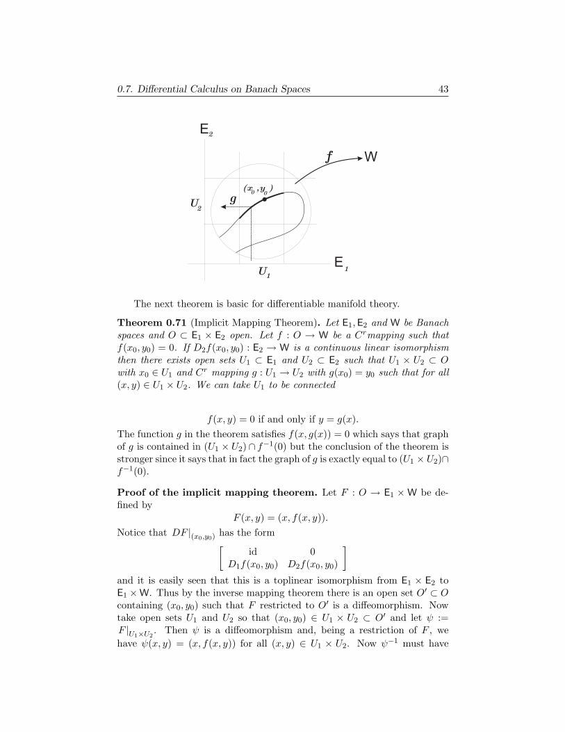
0.7. Differential Calculus on Banach Spaces 43
(x ,y )0 0
U
U
11
2
2
E
E
Wf
g
The next theorem is basic for differentiable manifold theory.
Theorem 0.71 (Implicit Mapping Theorem). Let E1,E2 and W be Banachspaces and O ⊂ E1 × E2 open. Let f : O → W be a Crmapping such thatf(x0, y0) = 0. If D2f(x0, y0) : E2 → W is a continuous linear isomorphismthen there exists open sets U1 ⊂ E1 and U2 ⊂ E2 such that U1 × U2 ⊂ Owith x0 ∈ U1 and Cr mapping g : U1 → U2 with g(x0) = y0 such that for all(x, y) ∈ U1 × U2. We can take U1 to be connected
f(x, y) = 0 if and only if y = g(x).The function g in the theorem satisfies f(x, g(x)) = 0 which says that graphof g is contained in (U1 × U2)∩ f−1(0) but the conclusion of the theorem isstronger since it says that in fact the graph of g is exactly equal to (U1 × U2)∩f−1(0).
Proof of the implicit mapping theorem. Let F : O → E1 ×W be de-fined by
F (x, y) = (x, f(x, y)).Notice that DF |(x0,y0) has the form
[id 0
D1f(x0, y0) D2f(x0, y0)
]
and it is easily seen that this is a toplinear isomorphism from E1 × E2 toE1 ×W. Thus by the inverse mapping theorem there is an open set O′ ⊂ Ocontaining (x0, y0) such that F restricted to O′ is a diffeomorphism. Nowtake open sets U1 and U2 so that (x0, y0) ∈ U1 × U2 ⊂ O′ and let ψ :=F |U1×U2
. Then ψ is a diffeomorphism and, being a restriction of F , wehave ψ(x, y) = (x, f(x, y)) for all (x, y) ∈ U1 × U2. Now ψ−1 must have
44 0. Background Material
the form ψ−1(x,w) = (x, h(x,w)) where h : ψ(U1 × U2) → U2. Note thatψ(U1 × U2) = U1 × h(U1 × U2).
Let g(x) := h(x, 0). Then (x, 0) = ψ ψ−1(x, 0) = ψ (x, h(x, 0)) =(x, f(x, h(x, 0))) so that in particular 0 = f(x, h(x, 0)) = f(x, g(x)) fromwhich we now see that graph(g) ⊂ (U1 × U2) ∩ f−1(0).
We now show that (U1 × U2) ∩ f−1(0) ⊂ graph(g). Suppose that forsome (x, y) ∈ U1 × U2 we have f(x, y) = 0. Then ψ(x, y) = (x, 0) and so
(x, y) = ψ−1 ψ(x, y)
= ψ−1(x, 0) = (x, h(x, 0))
= (x, g(x))
from which we see that y = g(x) and thus (x, y) ∈ graph(g). ¤
The simplest situation is that of a function f : R2 → R with f(a, b) = 0and D2f(a, b) 6= 0. Then the implicit mapping theorem gives a function g sothat f(x, g(x)) = 0 for all x sufficiently near a. Note, however, the followingexercise:
Exercise 0.72. Find a function f : R2 → R with D2f(0, 0) = 0 and acontinuous function g with f(x, g(x)) = 0 for all x sufficiently near a. Thuswe see that the implicit mapping theorem gives sufficient but not necessaryconditions for the existence of a function g with the property f(x, g(x)) = 0.
0.7.3. Immersion.
Theorem 0.73. Let E, and F be Banach spaces. Let U be and open subsetof E with 0 ∈ U , and let f : U → E× F be a smooth map with f(0) = (0, 0).If Df(0) : E → E × F is of the form x 7→ (α (x) , 0) for a continuous linearisomorphism α : E → E then there exists a diffeomorphism g from an openneighborhood V of (0, 0) ∈ E×F onto an an open neighborhood W of (0, 0) ∈E× F such that g f : f−1(V ) → W is of the form a 7→ (a, 0).
Proof. Define φ : U × F → E × F by φ(x, y) := f(x) + (0, y). Note thatφ(x, 0) = f(x) and Dφ(0, 0) = (α,idF) : x 7→ (α (x) , x) and this is clearlya continuous linear isomorphism. The inverse mapping theorem there is alocal inverse for φ say g : V → W . Thus if a is in U ′ we have
g f(a) = g (φ(a, 0)) = (a, 0)
¤
Corollary 0.74. If U is an open neighborhood of 0 ∈ Rk and f : U ⊂Rk → Rn is a smooth map with f(0) = 0 such that Df(0) has rank k then
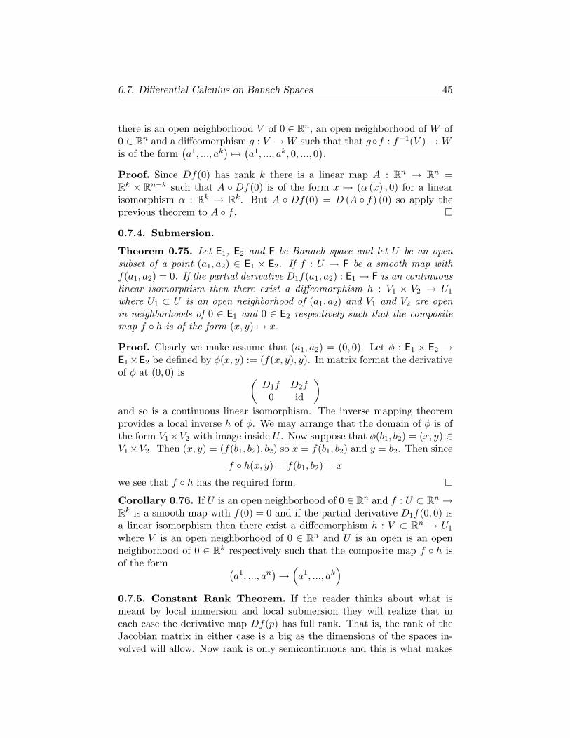
0.7. Differential Calculus on Banach Spaces 45
there is an open neighborhood V of 0 ∈ Rn, an open neighborhood of W of0 ∈ Rn and a diffeomorphism g : V → W such that that gf : f−1(V ) → Wis of the form
(a1, ..., ak
) 7→ (a1, ..., ak, 0, ..., 0
).
Proof. Since Df(0) has rank k there is a linear map A : Rn → Rn =Rk × Rn−k such that A Df(0) is of the form x 7→ (α (x) , 0) for a linearisomorphism α : Rk → Rk. But A Df(0) = D (A f) (0) so apply theprevious theorem to A f . ¤
0.7.4. Submersion.
Theorem 0.75. Let E1, E2 and F be Banach space and let U be an opensubset of a point (a1, a2) ∈ E1 × E2. If f : U → F be a smooth map withf(a1, a2) = 0. If the partial derivative D1f(a1, a2) : E1 → F is an continuouslinear isomorphism then there exist a diffeomorphism h : V1 × V2 → U1
where U1 ⊂ U is an open neighborhood of (a1, a2) and V1 and V2 are openin neighborhoods of 0 ∈ E1 and 0 ∈ E2 respectively such that the compositemap f h is of the form (x, y) 7→ x.
Proof. Clearly we make assume that (a1, a2) = (0, 0). Let φ : E1 × E2 →E1×E2 be defined by φ(x, y) := (f(x, y), y). In matrix format the derivativeof φ at (0, 0) is (
D1f D2f0 id
)
and so is a continuous linear isomorphism. The inverse mapping theoremprovides a local inverse h of φ. We may arrange that the domain of φ is ofthe form V1×V2 with image inside U . Now suppose that φ(b1, b2) = (x, y) ∈V1×V2. Then (x, y) = (f(b1, b2), b2) so x = f(b1, b2) and y = b2. Then since
f h(x, y) = f(b1, b2) = x
we see that f h has the required form. ¤Corollary 0.76. If U is an open neighborhood of 0 ∈ Rn and f : U ⊂ Rn →Rk is a smooth map with f(0) = 0 and if the partial derivative D1f(0, 0) isa linear isomorphism then there exist a diffeomorphism h : V ⊂ Rn → U1
where V is an open neighborhood of 0 ∈ Rn and U is an open is an openneighborhood of 0 ∈ Rk respectively such that the composite map f h isof the form (
a1, ..., an) 7→
(a1, ..., ak
)
0.7.5. Constant Rank Theorem. If the reader thinks about what ismeant by local immersion and local submersion they will realize that ineach case the derivative map Df(p) has full rank. That is, the rank of theJacobian matrix in either case is a big as the dimensions of the spaces in-volved will allow. Now rank is only semicontinuous and this is what makes
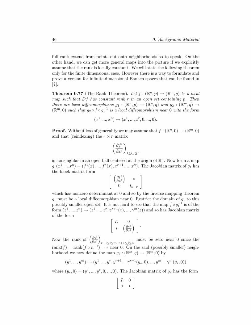
46 0. Background Material
full rank extend from points out onto neighborhoods so to speak. On theother hand, we can get more general maps into the picture if we explicitlyassume that the rank is locally constant. We will state the following theoremonly for the finite dimensional case. However there is a way to formulate andprove a version for infinite dimensional Banach spaces that can be found in[?].
Theorem 0.77 (The Rank Theorem). Let f : (Rn, p) → (Rm, q) be a localmap such that Df has constant rank r in an open set containing p. Thenthere are local diffeomorphisms g1 : (Rn, p) → (Rn, q) and g2 : (Rm, q) →(Rm, 0) such that g2 f g−1
1 is a local diffeomorphism near 0 with the form
(x1, ..., xn) 7→ (x1, ..., xr, 0, ..., 0).
Proof. Without loss of generality we may assume that f : (Rn, 0) → (Rm, 0)and that (reindexing) the r × r matrix
(∂f i
∂xj
)
1≤i,j≤r
is nonsingular in an open ball centered at the origin of Rn. Now form a mapg1(x1, ....xn) = (f1(x), ..., f r(x), xr+1, ..., xn). The Jacobian matrix of g1 hasthe block matrix form [ (
∂f i
∂xj
)∗
0 In−r
]
which has nonzero determinant at 0 and so by the inverse mapping theoremg1 must be a local diffeomorphism near 0. Restrict the domain of g1 to thispossibly smaller open set. It is not hard to see that the map f g−1
1 is of theform (z1, ..., zn) 7→ (z1, ..., zr, γr+1(z), ..., γm(z)) and so has Jacobian matrixof the form [
Ir 0∗
(∂γi
∂xj
)]
.
Now the rank of(
∂γi
∂xj
)r+1≤i≤m, r+1≤j≤n
must be zero near 0 since the
rank(f) = rank(f h−1) = r near 0. On the said (possibly smaller) neigh-borhood we now define the map g2 : (Rm, q) → (Rm, 0) by
(y1, ..., ym) 7→ (y1, ..., yr, yr+1 − γr+1(y∗, 0), ..., ym − γm(y∗, 0))
where (y∗, 0) = (y1, ..., yr, 0, ..., 0). The Jacobian matrix of g2 has the form[
Ir 0∗ I
]
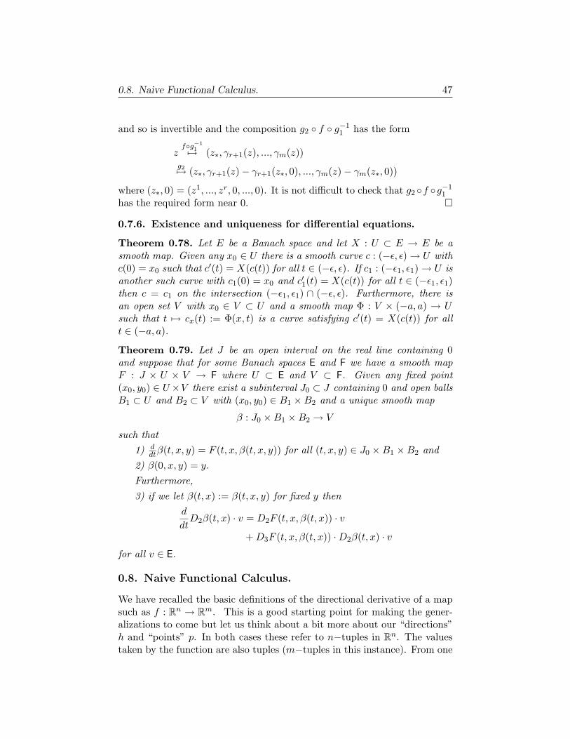
0.8. Naive Functional Calculus. 47
and so is invertible and the composition g2 f g−11 has the form
zfg−1
17→ (z∗, γr+1(z), ..., γm(z))g27→ (z∗, γr+1(z)− γr+1(z∗, 0), ..., γm(z)− γm(z∗, 0))
where (z∗, 0) = (z1, ..., zr, 0, ..., 0). It is not difficult to check that g2 f g−11
has the required form near 0. ¤
0.7.6. Existence and uniqueness for differential equations.
Theorem 0.78. Let E be a Banach space and let X : U ⊂ E → E be asmooth map. Given any x0 ∈ U there is a smooth curve c : (−ε, ε) → U withc(0) = x0 such that c′(t) = X(c(t)) for all t ∈ (−ε, ε). If c1 : (−ε1, ε1) → U isanother such curve with c1(0) = x0 and c′1(t) = X(c(t)) for all t ∈ (−ε1, ε1)then c = c1 on the intersection (−ε1, ε1) ∩ (−ε, ε). Furthermore, there isan open set V with x0 ∈ V ⊂ U and a smooth map Φ : V × (−a, a) → Usuch that t 7→ cx(t) := Φ(x, t) is a curve satisfying c′(t) = X(c(t)) for allt ∈ (−a, a).
Theorem 0.79. Let J be an open interval on the real line containing 0and suppose that for some Banach spaces E and F we have a smooth mapF : J × U × V → F where U ⊂ E and V ⊂ F. Given any fixed point(x0, y0) ∈ U×V there exist a subinterval J0 ⊂ J containing 0 and open ballsB1 ⊂ U and B2 ⊂ V with (x0, y0) ∈ B1 ×B2 and a unique smooth map
β : J0 ×B1 ×B2 → V
such that1) d
dtβ(t, x, y) = F (t, x, β(t, x, y)) for all (t, x, y) ∈ J0 ×B1 ×B2 and2) β(0, x, y) = y.
Furthermore,3) if we let β(t, x) := β(t, x, y) for fixed y then
d
dtD2β(t, x) · v = D2F (t, x, β(t, x)) · v
+ D3F (t, x, β(t, x)) ·D2β(t, x) · vfor all v ∈ E.
0.8. Naive Functional Calculus.
We have recalled the basic definitions of the directional derivative of a mapsuch as f : Rn → Rm. This is a good starting point for making the gener-alizations to come but let us think about a bit more about our “directions”h and “points” p. In both cases these refer to n−tuples in Rn. The valuestaken by the function are also tuples (m−tuples in this instance). From one
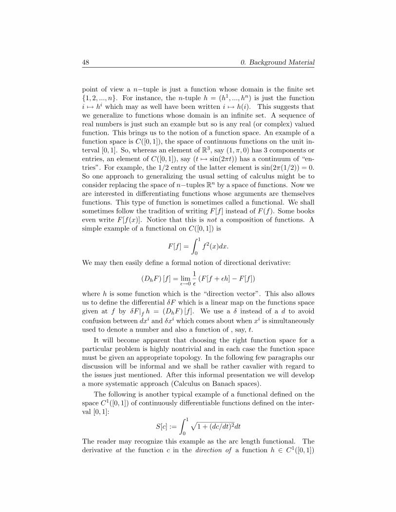
48 0. Background Material
point of view a n−tuple is just a function whose domain is the finite set1, 2, ..., n. For instance, the n-tuple h = (h1, ..., hn) is just the functioni 7→ hi which may as well have been written i 7→ h(i). This suggests thatwe generalize to functions whose domain is an infinite set. A sequence ofreal numbers is just such an example but so is any real (or complex) valuedfunction. This brings us to the notion of a function space. An example of afunction space is C([0, 1]), the space of continuous functions on the unit in-terval [0, 1]. So, whereas an element of R3, say (1, π, 0) has 3 components orentries, an element of C([0, 1]), say (t 7→ sin(2πt)) has a continuum of “en-tries”. For example, the 1/2 entry of the latter element is sin(2π(1/2)) = 0.So one approach to generalizing the usual setting of calculus might be toconsider replacing the space of n−tuples Rn by a space of functions. Now weare interested in differentiating functions whose arguments are themselvesfunctions. This type of function is sometimes called a functional. We shallsometimes follow the tradition of writing F [f ] instead of F (f). Some bookseven write F [f(x)]. Notice that this is not a composition of functions. Asimple example of a functional on C([0, 1]) is
F [f ] =∫ 1
0f2(x)dx.
We may then easily define a formal notion of directional derivative:
(DhF ) [f ] = limε→0
1ε
(F [f + εh]− F [f ])
where h is some function which is the “direction vector”. This also allowsus to define the differential δF which is a linear map on the functions spacegiven at f by δF |f h = (DhF ) [f ]. We use a δ instead of a d to avoidconfusion between dxi and δxi which comes about when xi is simultaneouslyused to denote a number and also a function of , say, t.
It will become apparent that choosing the right function space for aparticular problem is highly nontrivial and in each case the function spacemust be given an appropriate topology. In the following few paragraphs ourdiscussion will be informal and we shall be rather cavalier with regard tothe issues just mentioned. After this informal presentation we will developa more systematic approach (Calculus on Banach spaces).
The following is another typical example of a functional defined on thespace C1([0, 1]) of continuously differentiable functions defined on the inter-val [0, 1]:
S[c] :=∫ 1
0
√1 + (dc/dt)2dt
The reader may recognize this example as the arc length functional. Thederivative at the function c in the direction of a function h ∈ C1([0, 1])
0.8. Naive Functional Calculus. 49
would be given by
δS|c (h) = limε→0
1ε
(S[c + εh]− S[c]) .
It is well known that if δS|c (h) = 0 for every h then c is a linear function;c(t) = at + b. The condition δS|c (h) = 0 = 0 (for all h) is often simplywritten as δS = 0. We shall have a bit more to say about this notationshortly. For examples like this one, the analogy with multi-variable calculusis summarized as
The index or argument becomes continuous: i à t
d-tuples become functions: xi à c(t)
Functions of a vector variable become functionals of functions: f(~x) Ã S[c]
Here we move from d−tuples (which are really functions with finite domain)to functions with a continuous domain. The function f of x becomes afunctional S of functions c.
We now exhibit a common example from the mechanics which comesfrom considering a bead sliding along a wire. We are supposed to be givena so called “Lagrangian function” L : R × R → R which will be the basicingredient in building an associated functional. A typical example is of theform L(x, v) = 1
2mv2 − V (x). Define the action functional S by using L asfollows: For a given function t 7−→ q(t) defined on [a, b] let
S[q] :=∫ b
aL(q(t), q(t))dt.
We have used x and v to denote variables of L but since we are eventuallyto plug in q(t), q(t) we could also follow the common tradition of denotingthese variables by q and q but then it must be remembered that we are usingthese symbols in two ways. In this context, one sometimes sees somethinglike following expression for the so-called variation
(0.1) δS =∫
δS
δq(t)δq(t)dt
Depending on one’s training and temperament, the meaning of the notationmay be a bit hard to pin down. First, what is the meaning of δq as opposedto, say, the differential dq? Second, what is the mysterious δS
δq(t)? A goodstart might be to go back and settle on what we mean by the differential inordinary multivariable calculus. For a differentiable function f : Rd→ R wetake df to just mean the map
df : Rd × Rd→ R
given by df(p, h) = f ′(p)h. We may also fix p and write df |p or df(p) for thelinear map h 7→ df(p, h). With this convention we note that dxi
∣∣p(h) = hi
50 0. Background Material
where h = (h1, ..., hd). Thus applying both sides of the equation
(0.2) df |p =∑ ∂f
∂xi(p) dxi
∣∣p
to some vector h we get
(0.3) f ′(p)h =∑ ∂f
∂xi(p)hi.
In other words, df |p = Dhf(p) = ∇f · h = f ′(p). Too many notations forthe same concept. Equation 0.2 is clearly very similar to δS =
∫δS
δq(t)δq(t)dt
and so we expect that δS is a linear map and that t 7→ δSδq(t) is to δS as ∂f
∂xi
is to df :
df à δS
∂f
∂xià δS
δq(t).
Roughly, δSδq(t) is taken to be whatever function (or distribution) makes the
equation 0.1 true. We often see the following type of calculation
δS = δ
∫Ldt
=∫
(∂L
∂qδq +
∂L
∂qδq)dt
=∫∂L
∂q− d
dt
∂L
∂qδqdt(0.4)
from which we are to conclude thatδS
δq(t)=
∂L
∂q− d
dt
∂L
∂q
Actually, there is a subtle point here in that we must restrict δS to variationsfor which the integration by parts is justified. We can make much bettersense of things if we have some notion of derivative for functionals defined onsome function space. There is also the problem of choosing an appropriatefunction space. On the one hand, we want to be able to take (ordinary)derivatives of these functions since they may appear in the very definitionof S. On the other hand, we must make sense out of limits so we must picka space of functions with a tractable and appropriate topology. We will seebelow that it is very desirable to end up with what is called a Banach space.Often one is forced to deal with more general topological vector spaces. Letus ignore all of these worries for a bit longer and proceed formally. If δS issomehow the variation due to a variation h(t) of q(t) then it depends on boththe starting position in function space (namely, the function q(.)) and alsothe direction in function space that we move ( which is the function h(.)).
0.8. Naive Functional Calculus. 51
Thus we interpret δq = h as some appropriate function and then interpretδS as short hand for
δS|q(.) h := limε→0
1ε(S[q + εh]− S[q])
=∫
(∂L
∂qh +
∂L
∂qh)dt
Note: Here and throughout the book the symbol “:= ” is sued to indicateequality by definition.
If we had been less conventional and more cautious about notation wewould have used c for the function which we have been denoting by q : t 7→q(t). Then we could just write δS|c instead of δS|q(.). The point is that thenotation δS|q might leave one thinking that q ∈ R (which it is under oneinterpretation!) but then δS|q would make no sense. It is arguably better toavoid letting q refer both to a number and to a function even though this isquite common. At any rate, from here we restrict attention to “directions”h for which h(a) = h(b) = 0 and use integration by parts to obtain
δS|q(.) h =∫ ∂L
∂xi(q(t), q(t))− d
dt
∂L
∂q(q(t), q(t))hi(t)dt.
So it seems that the function E(t) := ∂L∂q (q(t), q(t))− d
dt∂L∂qi (q(t), q(t)) is the
right candidate for the δSδq(t) . However, once again, we must restrict to h
which vanish at the boundary of the interval of integration. On the otherhand, this family is large enough to force the desired conclusion. Despite thisrestriction the function E(t) is clearly important. For instance, if δS|q(.) = 0(or even δS|q(.) h = 0 for all functions that vanish at the end points) thenwe may conclude easily that E(t) ≡ 0. This gives an equation (or systemof equations) known as the Euler-Lagrange equation for the function q(t)corresponding to the action functional S :
∂L
∂q(q(t), q(t))− d
dt
∂L
∂q(q(t), q(t)) = 0
Exercise 0.80. Replace S[c] =∫
L(c(t), c(t))dt by the similar function ofseveral variables S(c1, ...cN ) =
∑L(ci,4ci). Here 4ci := ci − ci−1 (taking
c0 = cN ) and L is a differentiable map RN × RN→ R. What assumptions
52 0. Background Material
on c = (c1, ...cN ) and h = (h1, ...hN ) justify the following calculation?
dS|(c1,...cN ) h =∑ ∂L
∂cihi +
∂L
∂4ci4hi
=∑ ∂L
∂cihi +
∑ ∂L
∂4cihi −
∑ ∂L
∂4cihi−1
=∑ ∂L
∂cihi +
∑ ∂L
∂4cihi −
∑ ∂L
∂4ci+1hi
=∑ ∂L
∂cihi −
∑(
∂L
∂4ci+1− ∂L
∂4ci)hi
=∑
∂L
∂cihi − (4 ∂L
∂4ci)hi
=∑ ∂S
∂cihi.
The upshot of our discussion is that the δ notation is just an alternativenotation to refer to the differential or derivative. Note that qi might refer toa coordinate or to a function t 7→ qi(t) and so dqi is the usual differential andmaps Rd to R whereas δxi(t) is either taken as a variation function hi(t) asabove or as the map h 7→ δqi(t)(h) = hi(t). In the first interpretation δS =∫
δSδqi(t)
δqi(t)dt is an abbreviation for δS(h) =∫
δSδqi(t)
hi(t)dt and in the sec-
ond interpretation it is the map∫
δSδqi(t)
δqi(t)dt : h 7→ ∫δS
δqi(t)(δqi(t)(h))dt =∫
δSδqi(t)
hi(t)dt. The various formulas make sense in either case and bothinterpretations are ultimately equivalent. This much the same as taking thedxi in df = ∂f
∂xidxi to be components of an arbitrary vector (dx1, ..., dxd)or we may take the more modern view that dxi is a linear map given bydxi : h 7→ hi. If this seems strange recall that xi itself is also interpretedboth as a number and as a coordinate function.
Example 0.81. Let F [c] :=∫[0,1] c
2(t)dt as above and let c(t) = t3 andh(t) = sin(t4). Then
δF |c (h) = DhF (c) = limε→0
1ε
(F [c + εh]− F [c])
=d
dε
∣∣∣∣ε=0
F [c + εh]
=d
dε
∣∣∣∣ε=0
∫
[0,1](c(t)) + εh(t))2dt
= 2∫
[0,1]c(t)h(t)dt = 2
∫ 1
0t3 sin(πt4)dx
=1π
0.8. Naive Functional Calculus. 53
Note well that h and c are functions but here they are, more importantly,“points” in a function space! What we are differentiating is F . Again, F [c] isnot a composition of functions; the function c itself is the dependent variablehere.
Exercise 0.82. Notice that for a smooth function s : R→R we may write
∂s
∂xi(x0) = lim
h→0
s(x0 + hei)− s(x0)h
where ei = (0, ..., 1, ...0)
Consider the following similar statement which occurs in the physics litera-ture quite often.
δS
δc(t)= lim
h→0
S[c + hδt]− S[c]h
Here δt is the Dirac delta function (distribution) with the defining property∫δtφ = φ(t) for all continuous φ. To what extent is this rigorous? Try a
formal calculation using this limit to determine δSδc(t) in the case that
S(c) :=∫ 1
0c3(t)dt.
0.8.1. Lagrange Multipliers and Ljusternik’s Theorem. Note: Thissection is under construction.
The next example show how to use Lagrange multipliers to handle con-straints.
Example 0.83. Let E and F and F0 be as in the previous example. Wedefine two functionals
F [f ] :=∫
D∇f · ∇fdx
C[f ] =∫
Df2dx
We want a necessary condition on f such that f extremizes D subject tothe constraint C[f ] = 1. The method of Lagrange multipliers applies hereand so we have the equation DF|f = λ DC|f which means that
〈δFδf
, h〉 = λ〈δCδf
, h〉 for all h ∈ C2c (D)
orδFδf
= λδCδf
After determining the functional derivatives we obtain
−∇2f = λf
54 0. Background Material
This is not a very strong result since it is only a necessary condition andonly hints at the rich spectral theory for the operator ∇2.
Theorem 0.84. Let E and F be Banach spaces and U ⊂ E open with adifferentiable map f : U → F. If for x0 ∈ U with y0 = f(x0) we have thatDf |x0
is onto and ker Df |x0is complemented in E then the set x0+ker Df |x0
is tangent to the level set f−1(y0) in the following sense: There exists aneighborhood U ′ ⊂ U of x0 and a homeomorphism φ : U ′ → V where V isanother neighborhood of x0 and where φ(x0 + h) = x0 + h + ε(h) for somecontinuous function ε with the property that
limh→0
‖ε(h)‖‖h‖ = 0.
Proof. Df |x0is surjective. Let K := ker Df |x0
and let L be the comple-ment of K in E. This means that there are projections p : E → K andq : E → L
p2 = p and q2 = q
p + q = id
Let r > 0 be chosen small enough that x0 + Br(0) + Br(0) ⊂ U . Define amap
ψ : K ∩Br(0)× L ∩Br(0) → F
by ψ(h1, h2) := f(x0 + h1 + h2) for h1 ∈ K ∩ Br(0) and h2 ∈ L ∩ Br(0).We have ψ(0, 0) = f(x0) = y0 and also one may verify that ψ is C1 with∂1ψ = Df(x0)|K = 0 and ∂2ψ = Df(x0)|L. Thus ∂2ψ : L → F is acontinuous isomorphism (use the open mapping theorem) and so we have acontinuous linear inverse (∂2ψ)−1 : F → L. We may now apply the implicitfunction theorem to the equation ψ(h1, h2) = y0 to conclude that there is alocally unique function ε : K ∩Bδ(0) → L for small δ > 0 (less than r) suchthat
ψ(h, ε(h)) = y0 for all h ∈ K ∩Bδ(0)
ε(0) = 0
Dε(0) = − (∂2ψ)−1 ∂1ψ|(0,0)
But since ∂1ψ = Df(x0)|K = 0 this last expression means that Dε(0) = 0and so
limh→0
‖ε(h)‖‖h‖ = 0
Clearly the map φ : (x0+K∩Bδ(0)) → F defined by φ(x0+h) := x0+h+ε(h)is continuous and also since by construction y0 = ψ(h, ε(h)) = φ(x0 + h +ε(h)) we have that φ has its image in f−1(y0). Let the same symbol φ denotethe map φ : (x0 + K ∩Bδ(0)) → f−1(y0) which only differs in its codomain.
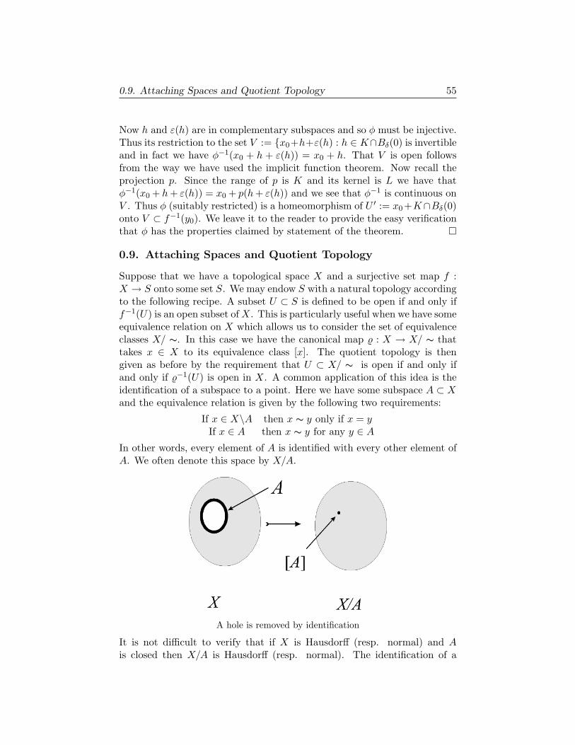
0.9. Attaching Spaces and Quotient Topology 55
Now h and ε(h) are in complementary subspaces and so φ must be injective.Thus its restriction to the set V := x0+h+ε(h) : h ∈ K∩Bδ(0) is invertibleand in fact we have φ−1(x0 + h + ε(h)) = x0 + h. That V is open followsfrom the way we have used the implicit function theorem. Now recall theprojection p. Since the range of p is K and its kernel is L we have thatφ−1(x0 + h + ε(h)) = x0 + p(h + ε(h)) and we see that φ−1 is continuous onV . Thus φ (suitably restricted) is a homeomorphism of U ′ := x0+K∩Bδ(0)onto V ⊂ f−1(y0). We leave it to the reader to provide the easy verificationthat φ has the properties claimed by statement of the theorem. ¤
0.9. Attaching Spaces and Quotient Topology
Suppose that we have a topological space X and a surjective set map f :X → S onto some set S. We may endow S with a natural topology accordingto the following recipe. A subset U ⊂ S is defined to be open if and only iff−1(U) is an open subset of X. This is particularly useful when we have someequivalence relation on X which allows us to consider the set of equivalenceclasses X/ ∼. In this case we have the canonical map % : X → X/ ∼ thattakes x ∈ X to its equivalence class [x]. The quotient topology is thengiven as before by the requirement that U ⊂ X/ ∼ is open if and only ifand only if %−1(U) is open in X. A common application of this idea is theidentification of a subspace to a point. Here we have some subspace A ⊂ Xand the equivalence relation is given by the following two requirements:
If x ∈ X\A then x ∼ y only if x = yIf x ∈ A then x ∼ y for any y ∈ A
In other words, every element of A is identified with every other element ofA. We often denote this space by X/A.
A hole is removed by identification
It is not difficult to verify that if X is Hausdorff (resp. normal) and Ais closed then X/A is Hausdorff (resp. normal). The identification of a
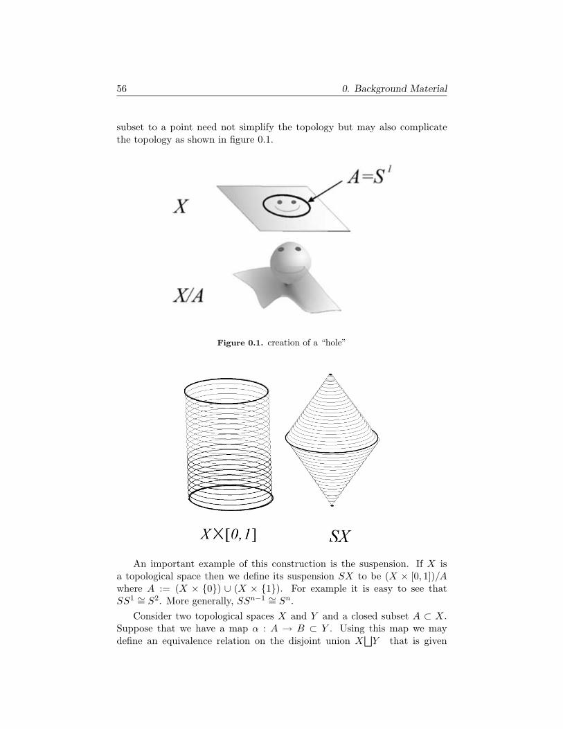
56 0. Background Material
subset to a point need not simplify the topology but may also complicatethe topology as shown in figure 0.1.
Figure 0.1. creation of a “hole”
An important example of this construction is the suspension. If X isa topological space then we define its suspension SX to be (X × [0, 1])/Awhere A := (X × 0) ∪ (X × 1). For example it is easy to see thatSS1 ∼= S2. More generally, SSn−1 ∼= Sn.
Consider two topological spaces X and Y and a closed subset A ⊂ X.Suppose that we have a map α : A → B ⊂ Y . Using this map we maydefine an equivalence relation on the disjoint union X
⊔Y that is given
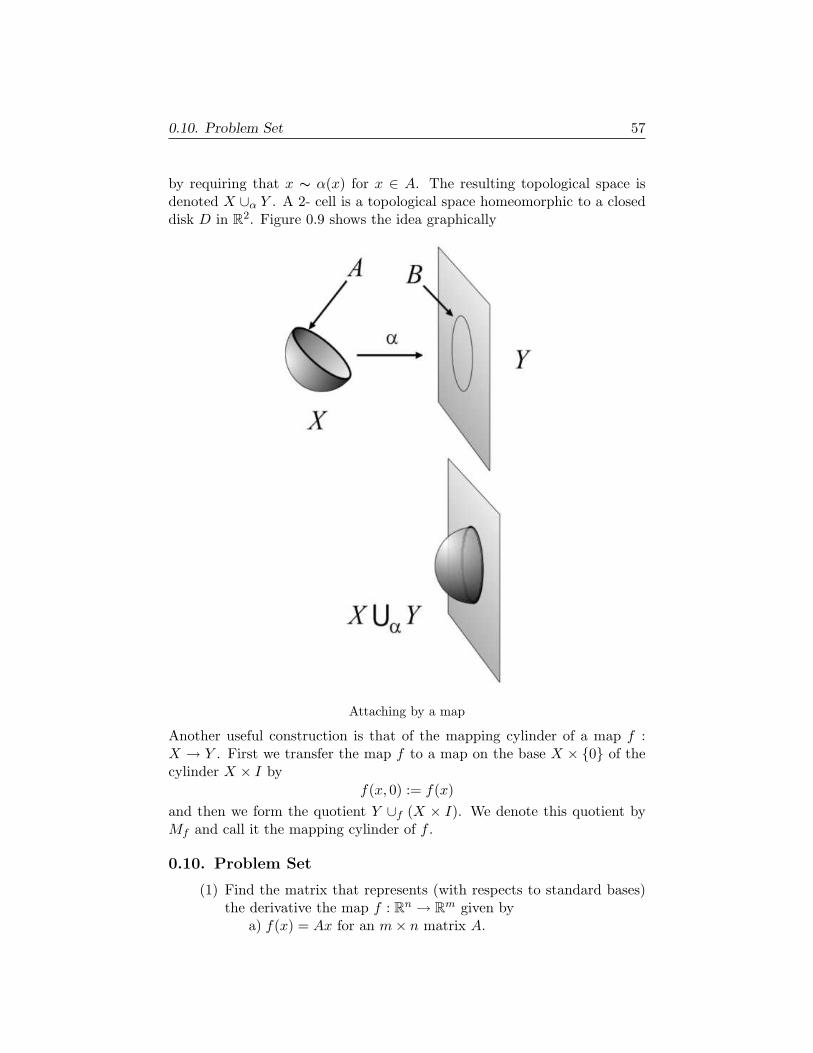
0.10. Problem Set 57
by requiring that x ∼ α(x) for x ∈ A. The resulting topological space isdenoted X ∪α Y . A 2- cell is a topological space homeomorphic to a closeddisk D in R2. Figure 0.9 shows the idea graphically
Attaching by a map
Another useful construction is that of the mapping cylinder of a map f :X → Y . First we transfer the map f to a map on the base X × 0 of thecylinder X × I by
f(x, 0) := f(x)and then we form the quotient Y ∪f (X × I). We denote this quotient byMf and call it the mapping cylinder of f .
0.10. Problem Set
(1) Find the matrix that represents (with respects to standard bases)the derivative the map f : Rn → Rm given by
a) f(x) = Ax for an m× n matrix A.
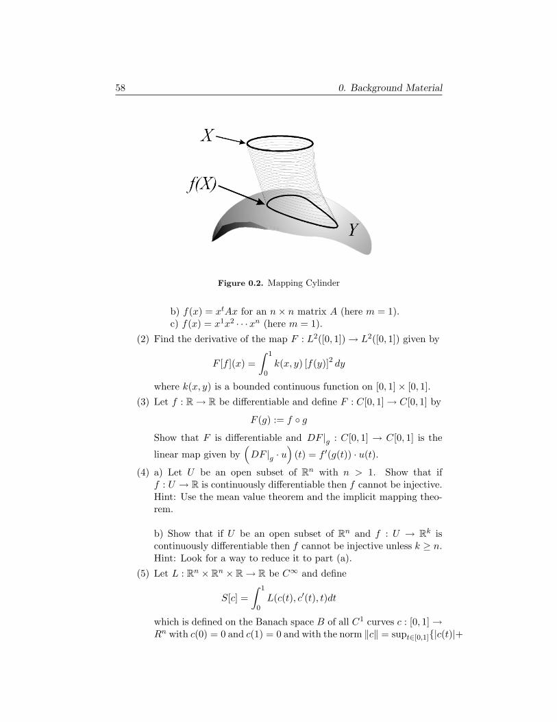
58 0. Background Material
Figure 0.2. Mapping Cylinder
b) f(x) = xtAx for an n× n matrix A (here m = 1).c) f(x) = x1x2 · · ·xn (here m = 1).
(2) Find the derivative of the map F : L2([0, 1]) → L2([0, 1]) given by
F [f ](x) =∫ 1
0k(x, y) [f(y)]2 dy
where k(x, y) is a bounded continuous function on [0, 1]× [0, 1].
(3) Let f : R→ R be differentiable and define F : C[0, 1] → C[0, 1] by
F (g) := f g
Show that F is differentiable and DF |g : C[0, 1] → C[0, 1] is the
linear map given by(
DF |g · u)
(t) = f ′(g(t)) · u(t).
(4) a) Let U be an open subset of Rn with n > 1. Show that iff : U → R is continuously differentiable then f cannot be injective.Hint: Use the mean value theorem and the implicit mapping theo-rem.
b) Show that if U be an open subset of Rn and f : U → Rk iscontinuously differentiable then f cannot be injective unless k ≥ n.Hint: Look for a way to reduce it to part (a).
(5) Let L : Rn × Rn × R→ R be C∞ and define
S[c] =∫ 1
0L(c(t), c′(t), t)dt
which is defined on the Banach space B of all C1 curves c : [0, 1] →Rn with c(0) = 0 and c(1) = 0 and with the norm ‖c‖ = supt∈[0,1]|c(t)|+
0.10. Problem Set 59
|c′(t)|. Find a function gc : [0, 1] → Rn such that
DS|c · b =∫ 1
0〈gc(t), b(t)〉dt
or in other words,
DS|c · b =∫ 1
0
n∑
i=1
gic(t)b
i(t)dt.
(6) In the last problem, if we had not insisted that c(0) = 0 and c(1) =0, but rather that c(0) = x0 and c(1) = x1, then the space wouldn’teven have been a vector space let alone a Banach space. But thisfixed endpoint family of curves is exactly what is usually consideredfor functionals of this type. Anyway, convince yourself that this isnot a serious problem by using the notion of an affine space (like avector space but no origin and only differences are defined).
Hint: If we choose a fixed curve c0 which is the point in theBanach space at which we wish to take the derivative then we canwrite B~x0~x1
= B + c0 where
B~x0~x1= c : c(0) = ~x0 and c(1) = ~x1
B = c : c(0) = 0 and c(1) = 0Then we have Tc0B~x0~x1
∼= B. Thus we should consider DS|c0 : B →B.
(7) Let Flt(.) be defined by Flt(x) = (t + 1)x for t ∈ (−1/2, 1/2) andx ∈ Rn. Assume that the map is jointly C1 in both variable. Findthe derivative of
f(t) =∫
D(t)(tx)2 dx
at t = 0 , where D(t) := Flt(D) the image of the disk D = |x| ≤ 1.Hint: Find the Jacobian Jt := det[DFlt(x)] and then convert
the integral above to one just over D(0) = D.
(8) Let Mn×n(R) be the vector space of n×n matrices with real entriesand let det : Mn×n(R) → R be the determinant map. The deriv-ative at the identity element I should be a linear map D det(I): Mn×n(R) → R. Show that D det(I) ·B = Tr(B). More generally,show that D det(A) ·B = Tr((cof A)t B) where cof A is the matrixof cofactors of A.
What is ∂∂xij
det X where X = (xij) ?
(9) Let A : U ⊂ E → L(F,F) be a Cr map and define F : U × F → Fby F (u, f) := A(u)f . Show that F is also Cr.
60 0. Background Material
(10) Show that if F is any closed subset of Rn there is a C∞-function fwhose zero set x : f(x) = 0 is exactly F .
(11) Let U be an open set in Rn. For f ∈ Ck(U) and S ⊂ U a compactset, let ‖f‖S
k :=∑|α|≤k supx∈S
∣∣∣∂|α|f∂xα (x)
∣∣∣. a) Show that (1) ‖rf‖Sk =
|r| ‖f‖Sk for any r ∈ R, (2) ‖f1 + f2‖S
k ≤ ‖f1‖Sk + ‖f2‖S
k for anyf1, f2 ∈ Ck(U), (3) ‖fg‖S
k ≤ ‖f‖Sk ‖g‖S
k for f, g ∈ Ck(U).b) Let Ki be a compact subsets of U such that U =
⋃i Ki. Show
that d(f, g) :=∑∞
i=012i
‖f−g‖Kik
1+‖f−g‖Kik
defines a complete metric space
structure on Ck(U).(12) Let E and F be real Banach spaces. A function f : E → F is said
to be homogeneous of degree k if f(rx) = rf(x) for all r ∈ Rand x ∈ E. Show that if f is homogeneous of degree k and isdifferentiable, then Df(v) · v = kf(v).
(13) Show that the implicit mapping theorem implies the inverse map-ping theorem. Hint: Consider g(x, y) = f(x)− y for f : U → F.
Chapter 1
Chapter 1 Supplement
1.1. Comments and Errata
1.1.1. Comments. (Nothing yet)
1.1.2. Errata. (Nothing yet)
1.2. Rough Ideas I
The space of n-tuples Rn is often called Euclidean space by mathematiciansbut it might be a bit more appropriate the refer to this a Cartesian spacewhich is what physics people often call it. The point is that Euclideanspace (denoted here as En) has both more structure and less structure thanCartesian space. More since it has a notion of distance and angle, lessbecause Euclidean space as it is conceived of in pure form has no origin orspecial choice of coordinates. Of course we almost always give Rn it usualstructure as an inner product space from which we get the angle and distanceand we are on our way to having a set theoretic model of Euclidean space.
Let us imagine we have a pure Euclidean space. The reader shouldthink physical of space as it is normally given to intuition. Rene de Cartesshowed that if this intuition is axiomatized in a certain way then the resultingabstract space may be put into one to one correspondence with the set ofn-tuples, the Cartesian space Rn. There is more than one way to do this butif we want the angle and distance to match that given by the inner productstructure on Rn then we get the so called rectilinear coordinates familiar toall users of mathematics.
61
62 1. Chapter 1 Supplement
After imposing rectilinear coordinates on a Euclidean space En (such asthe plane E2) we identify Euclidean space with Rn, the vector space of n-tuples of numbers. In fact, since a Euclidean space in this sense is an objectof intuition (at least in 2d and 3d) some may insist that to be sure such aspace of points really exists that we should in fact start with Rn and “forget”the origin and all the vector space structure while retaining the notion ofpoint and distance. The coordinatization of Euclidean space is then just a“remembering” of this forgotten structure. Thus our coordinates arise froma map x : En → Rn which is just the identity map. This approach has muchto recommend it and we shall more or less follow this canonical path. Thereis at least one regrettable aspect to this approach which is the psychologicaleffect that results from always picturing Euclidean space as Rn. The result isthat when we introduce the idea of a manifold and describe what coordinatesare in that setting it seems like a new idea. It might seem that this isa big abstraction and when the definition of charts and atlases and so onappear a certain notational fastidiousness sets in that somehow creates apsychological gap between open sets in Rn and the abstract space that wecoordinatize. But what is now lost from sight is that we have already beendealing with an abstract manifolds En which we have identified with Rn viaexactly such an idea of coordinates. Euclidean space was already always amanifold. But Euclidean space could just as easily support other coordinatessuch as spherical coordinates. In this case also we just get to work in thenew coordinates without pondering what the exact definition of a coordinatesystem should be. We also picture the coordinates as being “on the space”and not as a map to some other Euclidean space. But how else shouldcoordinates be defined? Consider how naturally a calculus student works invarious coordinate systems. What competent calculus student would wastetime thinking of polar coordinates as given by a map E2 → R2 (defined on aproper open subset of course) and then wonder whether something like drdθlives on the original En or in the image of the coordinate map En → Rn?It has become an unfortunate consequence of the modern viewpoint thatsimple geometric ideas are lost from the notation. Ideas that allow one tothink about “quantities and their variations” and then comfortably writethings like
rdr ∧ dθ = dx ∧ dy
without wondering if this shouldn’t be a “pullback” ψ∗12(rdr∧dθ) = dx∧dywhere ψ12 is the change of coordinate map R2 → R2 given by
x(r, θ) = r cos θ
y(r, θ) = r cos θ
1.2. Rough Ideas I 63
Of course, the experienced differential geometer understands the variousmeanings and gleans from the context what the proper meaning of a no-tation should be. The new student of manifold theory on the other hand,is faced with a pedagogy that teaches notation, trains one to examine eachequation for logical self consistency, but fails to teach geometric intuition.Having made this complaint the author must confess that he too will use themodern notation and will not stray far from standard practice. The studentmust learn how differential geometry is actually done. These remarks aremeant to encourage the student to stop and seek the simplest most intuitiveviewpoint whenever feeling overwhelmed by notation. The student is en-couraged to experiment with abbreviated personal notation when checkingcalculations and to draw diagrams and schematics that encode the geomet-ric ideas whenever possible. The maxim should be “Let the geometry writethe equations”.
Now this approach works fine as long as intuition is not allowed to over-come logic and thereby mislead us. On occasion intuition does mislead usand this is where the pedantic notation and the various abstractions can saveus from error. The abstractions and pedantic notations are related to an-other issue: Why introduce abstract structures such as sheaves and modulesand so forth. Couldn’t differential geometry do without these notions beingexplicitly introduced? Perhaps, but there is a new force on the horizon thedemands that we have a very firm grip on the logical and algebraic aspectsof differential geometry. Namely, noncommutative geometry. Here the ideais to replace the algebra of continuous (and the subalgebra of smooth) func-tions by a noncommutative algebra. In this new setting one tries to studyanalogues of the objects of ordinary differential geometry. But this meanshaving a very good grip on the exact role in ordinary geometry of functionalgebras and the various modules over these algebras. Things that seem soobvious like the naturality with respect to restrictions and so forth cannotbe taken for granted, indeed, may not even have a meaning in the new worldof noncommutative geometry. This is one reason that we shall not shy awayfrom certain ideas such as the relation between finitely generated modules,locally free sheaves and vector bundles. We also intend to be a bit morepedantic than usual when we do tensor analysis1. What of the differencebetween V ⊗ V ∗ and V ∗ ⊗ V ; should they be identified?
1What about the choice of writing coefficients on the right or left in linear expressions. Should
the tensor algebra distinguish Tij∣∣kl
from T jikl? Is the covariant differential ∇T of a tensor T ∈ Γ(
TM ⊗ TM∗) be thought of as an element of Γ(TM ⊗ TM∗ ⊗ TM∗) as the notation T ij;k suggests
or as an element of Γ(TM∗ ⊗ TM ⊗ TM∗) as the notation ∇iTij suggests? What effect does this
have on the sign convention for the curvatuire tensor. If you think it doesn’t matter ask yourselfif you are still sure about that in the noncommutative setting.
64 1. Chapter 1 Supplement
So, as we said, after imposing rectilinear coordinates on a Euclideanspace En (such as the plane E2) we identify Euclidean space with Rn, thevector space of n−tuples of numbers. We will envision there to be a copyRn
p of Rn at each of its points p ∈ Rn. One way to handle this is to setRn
p = p × Rn so that taking all points of a domainU into account weshould consider U × Rn. Thus if (p, v) ∈ U × Rn we take this to representthe vector at p which is parallel to v. The elements of Rn
p are to be thoughtof as the vectors based at p, that is, the “tangent vectors”. These tangentspaces are related to each other by the obvious notion of vectors beingparallel (this is exactly what is not generally possible for tangents spaces ofa manifold). For the standard basis vectors ej (relative to the coordinates
xi) taken as being based at p we often write ∂∂xi
∣∣∣p
instead of (p, ej) and this
has the convenient second interpretation as a differential operator acting onC∞functions defined near p ∈ Rn. Namely,
∂
∂xi
∣∣∣∣p
f =∂f
∂xi(p).
An n-tuple of C∞functions X1, ..., Xn defines a C∞vector field X =∑
Xi ∂∂xi
whose value at p is∑
Xi(p) ∂∂xi
∣∣∣p. Thus a vector field assigns to each p in
its domain, an open set U , a vector∑
Xi(p) ∂∂xi
∣∣∣p
at p. We may also think
of vector field as a differential operator via
f 7→ Xf ∈ C∞(U)
(Xf)(p) :=∑
Xi(p)∂f
∂xi(p)
Example 1.1. X = y ∂∂x − x ∂
∂y is a vector field defined on U = R2 − 0and (Xf)(x, y) = y ∂f
∂x (x, y)− x∂f∂y (x, y).
Notice that we may certainly add vector fields defined over the sameopen set as well as multiply by functions defined there:
(fX + gY )(p) = f(p)X(p) + g(p)X(p)
The familiar expression df = ∂f∂x1
dx1 + · · ·+ ∂f∂xn
dxn has the intuitive in-terpretation expressing how small changes in the variables of a function giverise to small changes in the value of the function. Two questions should cometo mind. First, “what does ‘small’ mean and how small is small enough?”Second, “which direction are we moving in the coordinate” space? The an-swer to these questions lead to the more sophisticated interpretation of dfas being a linear functional on each tangent space. Thus we must choose adirection vp at p ∈ Rn and then df(vp) is a number depending linearly on
1.2. Rough Ideas I 65
our choice of vector vp. The definition is determined by dxi( ∂∂xi
∣∣∣p) = δij . In
fact, this shall be the basis of our definition of df at p. We want
df |p (∂
∂xi
∣∣∣∣p
) :=∂f
∂xi(p).
Now any vector at p may be written vp =∑n
i=1 vi ∂∂xi
∣∣∣p
which invites us
to use vp as a differential operator (at p):
vpf :=n∑
i=1
vi ∂f
∂xi(p) ∈ R
This consistent with our previous statement about a vector field being adifferential operator simply because X(p) = Xp is a vector at p for everyp ∈ U . This is just the directional derivative. In fact we also see that
df |p (vp) =∑
j
∂f
∂xj(p)dxj
(n∑
i=1
vi ∂
∂xi
∣∣∣∣p
)
=n∑
i=1
vi ∂f
∂xi(p) = vpf
so that our choices lead to the following definition:
Definition 1.2. Let f be a C∞function on an open subset U of Rn. By thesymbol df we mean a family of maps df |p with p varying over the domainU of f and where each such map is a linear functional of tangent vectorsbased at p given by df |p (vp) = vpf =
∑ni=1 vi ∂f
∂xi(p).
Definition 1.3. More generally, a smooth 1-form α on U is a family oflinear functionals αp : TpRn → R with p ∈ U that is smooth is the sense
that αp( ∂∂xi
∣∣∣p) is a smooth function of p for all i.
From this last definition it follows that if X = Xi ∂∂xi
is a smooth vectorfield then α(X)(p) := αp(Xp) defines a smooth function of p. Thus analternative way to view a 1−form is as a map α : X 7→ α(X) that is definedon vector fields and linear over the algebra of smooth functions C∞(U) :
α(fX + gY ) = fα(X) + gα(Y ).
Fixing a problem. It is at this point that we want to destroy the priv-ilege of the rectangular coordinates and express our objects in an arbitrarycoordinate system smoothly related to the existing coordinates. This meansthat for any two such coordinate systems, say u1, ..., un and y1, ...., yn we
66 1. Chapter 1 Supplement
want to have the ability to express fields and forms in either system andhave for instance
Xi(y)
∂
∂yi= X = Xi
(u)
∂
∂ui
for appropriate functions Xi(y), Xi
(u). This equation only makes sense on theoverlap of the domains of the coordinate systems. To be consistent with thechain rule we must have
∂
∂yi=
∂uj
∂yi
∂
∂uj
which then forces the familiar transformation law:∑ ∂uj
∂yiXi
(y) = Xi(u)
We think of Xi(y) and Xi
(u) as referring to, or representing, the same geo-metric reality from the point of view of two different coordinate systems.No big deal right? Well, how about the fact, that there is this underlyingabstract space that we are coordinatizing? That too is no big deal. Wewere always doing it in calculus anyway. What about the fact that the co-ordinate systems aren’t defined as a 1-1 correspondence with the points ofthe space unless we leave out some points in the space? For example, polarcoordinates must exclude the positive x-axis and the origin in order to avoidambiguity in θ and have a nice open domain. Well if this is all fine then wemay as well imagine other abstract spaces that support coordinates in thisway. This is manifold theory. We don’t have to look far for an example ofa manifold other than Euclidean space. Any surface such as the sphere willdo. We can talk about 1-forms like say α = θdφ + φ sin(θ)dθ, or a vectorfield tangent to the sphere θ sin(φ) ∂
∂θ + θ2 ∂∂φ and so on (just pulling things
out of a hat). We just have to be clear about how these arise and most of allhow to change to a new coordinate expression for the same object. This isthe approach of tensor analysis. An object called a 2-tensor T is representedin two different coordinate systems as for instance
∑T ij
(y)
∂
∂yi⊗ ∂
∂yj=
∑T ij
(u)
∂
∂ui⊗ ∂
∂uj
where all we really need to know for many purposes the transformation law
T ij(y) =
∑r,s
T rs(u)
∂yi
∂ur
∂yi
∂us.
Then either expression is referring to the same abstract tensor T . This isjust a preview but it highlight the approach wherein a transformation lawsplay a defining role.
In order to understand modern physics and some of the best mathematicsit is necessary to introduce the notion of a space (or spacetime) that only
1.2. Rough Ideas I 67
locally has the (topological) features of a vector space like Rn. Examplesof two dimensional manifolds include the sphere or any of the other closedsmooth surfaces in R3 such a torus. These are each locally like R2 andwhen sitting in space in a nice smooth way like we usually picture them,they support coordinates systems that allow us to do calculus on them. Thereader will no doubt be comfortable with the idea that it makes sense totalk about directional rates of change in say a temperature distribution ona sphere representing the earth.
For a higher dimensional example we have the 3−sphere S3 which is thehypersurface in R4 given by the equation x2 + y2 + z2 + w2 = 1.
For various reasons, we would like coordinate functions to be defined onopen sets. For closed surfaces like the sphere, it is not possible to definenice coordinates that are defined on the whole surface. By nice we meanthat together the coordinate functions, say, θ, φ should combine to give a 1-1correspondence with a subset of R2 that is continuous and has a continuousinverse. In general the best we can do is introduce several coordinate systemseach defined on separate open subsets that together cover the surface. Thiswill be the general idea for all manifolds.
Now suppose that we have some surface S and two coordinate systems
(θ, φ) : U1 → R2
(u, v) : U2 → R2
Imagine a real valued function f defined on S (think of f as temperature).Now if we write this function in coordinates (θ, φ) we have f represented bya function of two variables f1(θ, φ) and we may ask if this function is dif-ferentiable or not. On the other hand, f is given in (u, v) coordinates by arepresentative function f2(u, v). In order that our conclusions about differ-entiability at some point p ∈ U1 ∩U2 ⊂ S should not depend on what coor-dinate system we use we had better have the coordinate systems themselvesrelated differentiably. That is, we want the coordinate change functionsin both directions to be differentiable. For example we may then relate thederivatives as they appear in different coordinates by chain rules expressionslike
∂f1
∂θ=
∂f2
∂u
∂u
∂θ+
∂f2
∂v
∂v
∂θwhich have validity on coordinate overlaps. The simplest and most usefulcondition to require is that coordinates systems have C∞ coordinate changeson the overlaps.
Definition 1.4. A set M is called a C∞differentiable manifold of dimensionn if M is covered by the domains of some family of coordinate mappings orcharts xα : Uα → Rnα∈A where xα = (x1
α, x2α, .....xn
α). We require that the
68 1. Chapter 1 Supplement
coordinate change maps xβ x−1α are continuously differentiable any number
of times on their natural domains in Rn. In other words, we require thatthe functions
x1 = x1β(x1
α, ..., xnα)
x2β = x2
β(x1α, ..., xn
α)...
xnβ = xn
β(x1α, ..., xn
α)
together give a C∞ bijection where defined. The α and β are just indicesfrom some set A and are just a notational convenience for naming the indi-vidual charts.
Note that we are employing the same type of abbreviations and abuse ofnotation as is common is every course on calculus where we often write thingslike y = y(x). Namely, (x1
α, ..., xnα) denotes both an n-tuple of coordinate
functions and an element of Rn. Also, x1β = x1
β(x1α, ..., xn
α) etc. could bethought of as an abbreviation for a functional relation that when evaluatedat a point p on the manifold reads
(x1β(p), .....xn
β(p)) = xβ x−1α (x1
α(p), ..., xnα(p)).
A function f on M will be deemed to be Cr if its representatives fα areall Cr for every coordinate system xα = (x1
α, ..., xnα) whose domain intersects
the domain of f . Now recall our example of temperature on a surface. Foran arbitrary pair of coordinate systems x = (x1, ..., xn) and y = (y1, ..., yn)the functions f1 := f x−1 and f2 := f y−1 represent the same functionf with in the coordinate domains but the expressions ∂f1
∂xi and ∂f2
∂yi are notequal and do not refer to the same physical or geometric reality. The pointis simply that because of our requirements on the smooth relatedness ofour coordinate systems we know that on the overlap of the two coordinatesystems if f x−1 has continuous partial derivatives up to order k then thesame will be true of f y−1.
1.3. Pseudo-Groups and Models Spaces
Without much work we can generalize our definitions in such a way as toprovide, as special cases, the definition of some common notions such as thatcomplex manifold and manifold with boundary. If fact, we would also liketo include infinite dimensional manifolds. An infinite dimensional manifoldis modeled on an infinite dimensional Banach space. It is quite importantfor our purposes to realize that the spaces (so far just Rn) that will be themodel spaces on which we locally model our manifolds should have a distin-guished family of local homeomorphisms. For example, Cr−differentiable
1.3. Pseudo-Groups and Models Spaces 69
manifolds are modeled on Rn where on the latter space we single out thelocal Cr−diffeomorphisms between open sets. But we also study complexmanifolds, foliated manifolds, manifolds with boundary, Hilbert manifoldsand so on. Thus we need appropriate model spaces but also, significantly,we need a distinguished family on maps on the space. In this context thefollow notion becomes useful:
Definition 1.5. A pseudogroup of transformations, say G, of a topo-logical space X is a family Φγγ∈Γ of homeomorphisms with domain Uγ
and range Vγ both open subsets of X, that satisfies the following properties:1) idX ∈ G.2) For all Φγ ∈ G and open U ⊂ Uγ the restrictions Φγ |U are in G .
3) fγ ∈ G implies f−1γ ∈ G
4) The composition of elements of G are elements of G whenever thecomposition is defined with nonempty domain.
5) For any subfamily Φγγ∈G1 ⊂ G such that Φγ |Uγ∩Uν= Φν |Uγ∩Uν
whenever Uγ ∩ Uν 6= ∅ then the mapping defined by Φ :⋃
γ∈G1Uγ →⋃
γ∈G1Vγ is an element of G if it is a homeomorphism.
Definition 1.6. A sub-pseudogroup S of a pseudogroup is a subset of Gand is also a pseudogroup (and so closed under composition and inverses).
We will be mainly interested in Cr-pseudogroups and the spaces thatsupport them. Our main example will be the set Gr
Rn of all Cr maps betweenopen subsets of Rn. More generally, for a Banach space B we have theCr-pseudo-group Gr
B consisting of all Cr maps between open subsets of aBanach space B. Since this is our prototype the reader should spend sometime thinking about this example.
Definition 1.7. A Cr− pseudogroup of transformations of a subset M ofBanach space B is a pseudogroup arising as the restriction to M of a sub-pseudogroup of Gr
M. The set M with the relative topology and this Cr−pseudogroup is called a model space.
Example 1.8. Recall that a map U ⊂ Cn → Cn is holomorphic if thederivative (from the point of view of the underlying real space R2n) is infact complex linear. A holomorphic map with holomorphic inverse is calledbiholomorphic. The set of all biholomorphic maps between open subsets ofCn is a pseudogroup. This is a Cr-pseudogroup for all r including r = ω.In this case the subset M we restrict to is just Cn itself.
In the great majority of examples the subset M ⊂ V is in fact equalto V itself. One important exception to this will lead us to a convenientformulation of manifold with boundary. First we need a definition:
70 1. Chapter 1 Supplement
Definition 1.9. Let λ ∈ M∗ be a continuous from on a Banach space M.In the case of Rn it will be enough to consider projection onto the firstcoordinate x1. Now let M+
λ = x ∈ M: λ(x) ≥ 0 and M−λ = x ∈ M:
λ(x) ≤ 0 and ∂M+λ = ∂M−
λ = x ∈ M: λ(x) = 0 is the kernel of λ. ClearlyM+
λ and M−λ are homeomorphic and ∂M−
λ is a closed subspace. 2
Example 1.10. Let GrM−
λ
be the restriction to M−λ of the set of Cr-diffeomorphisms
φ from open subset of M to open subsets of M that have the following prop-erty
*) If the domain U of φ ∈ GrM has nonempty intersection with M0 :=
x ∈ M: λ(x) = 0 then φ|M0∩U : M0 ∩ U → M0 ∩ U .
Notation 1.11. It will be convenient to denote the model space for a man-ifold M (resp. N etc.) by M (resp. N etc.). That is, we use the same letterbut use the sans serif font (this requires the reader to be tuned into fontdifferences). There will be exceptions. One exception will be the case wherewe want to explicitly indicate that the manifold is finite dimensional andthus modeled on Rn for some n. Another exception will be when E is thetotal space of a vector bundle over M . In this case E will be modeled on aspace of the form M×E. This will be explained in detail when study vectorbundles.
Let us begin again redefine a few notions in greater generality. Let Mbe a topological space. An M-chart on M is a homeomorphism x whosedomain is some subset U ⊂ M and such that x(U) is an open subset of afixed model space M.
Definition 1.12. Let G be a Cr-pseudogroup of transformations on a modelspace M. A G-atlas for a topological space M is a family of charts xα, Uαα∈A
(where A is just an indexing set) that cover M in the sense that M =⋃α∈A Uα and such that whenever Uα ∩ Uβ is not empty then the map
xβ x−1α : xα(Uα ∩ Uβ) → xβ(Uα ∩ Uβ)
is a member of G. The maps xβ x−1α are called various things by various au-
thors including “transition maps”, “coordinate change maps”, and “overlapmaps”.
Now the way we set up the definition the model space M is a subset ofa Banach space. If M the whole Banach space (the most common situation)and if G = Gr
M (the whole pseudogroup of local Crdiffeomorphisms) then wejust call the atlas a Cr atlas.
2The reason we will use both E+ and E− in the following definition for a technical reasonhaving to do with the consistancy of our definition of induced orientation of the boundary.
1.3. Pseudo-Groups and Models Spaces 71
Exercise 1.13. Show that this definition of Cr atlas is the same as ouroriginal definition in the case where M is the finite dimensional Banachspace Rn.
In practice, a G−manifold is just a space M (soon to be a topologicalmanifold) together with an G−atlas A but as before we should tidy thingsup a bit for our formal definitions. First, let us say that a bijection onto anopen set in a model space, say x : U → x(U) ⊂ M, is compatible with theatlas A if for every chart xα, Uα from the atlas A we have that the compositemap
x x−1α : xα(Uα ∩ U) → xβ(Uα ∩ U)
is in Gr. The point is that we can then add this map in to form a largerequivalent atlas: A′ = A ∪ x, U. To make this precise let us say that twodifferent Cr atlases, say A and B are equivalent if every map from the firstis compatible (in the above sense) with the second and visa-versa. In thiscase A′ = A ∪ B is also an atlas. The resulting equivalence class is called aGr−structure on M .
Now it is clear that every equivalence class of atlases contains a uniquemaximal atlas which is just the union of all the atlases in the equivalenceclass. Of course every member of the equivalence class determines the max-imal atlas also–just toss in every possible compatible chart and we end upwith the maximal atlas again.
Definition 1.14. A topological manifold M is called a Cr−differentiablemanifold (or just Cr manifold) if it comes equipped with a differentiablestructure. M is given the topology induced by the maximal atlas for thegiven Cr differentiable structure. Whenever we speak of a differentiablemanifold we will have a fixed differentiable structure and therefore a maximalCr−atlas AM in mind. A chart from AM will be called an admissiblechart.
We started out with a topological manifold but if we had just startedwith a set M and then defined a chart to be a bijection x : U → x(U),only assuming x(U) to be open then a maximal atlas AM would generate atopology on M . Then the set U would be open. Of course we have to checkthat the result is a paracompact space but once that is thrown into our listof demand we have ended with the same notion of differentiable manifold.To see how this approach would go the reader should consult the excellentbook [?].
Now from the vantage point of this general notion of model space and thespaces modeled on them we get a slick definition of manifold with boundary.
Definition 1.15. A set M is called a Cr−differentiable manifold withboundary (or just Cr manifold with boundary) if it comes equipped with a
72 1. Chapter 1 Supplement
GrM−
λ
−structure. M is given the topology induced by the maximal atlas forthe given Gr
M−λ
structure. Whenever we speak of a Cr−manifold with bound-ary we will have a fixed Gr
M−λ
structure and therefore a maximal GrM−
λ
atlasAM in mind. A chart from AM will be called an admissible chart.
Remark 1.16. It may be the case that there are two or more differentdifferentiable structures on the same topological manifold. But see remark?? below.
Notice that the model spaces used in the definition of the charts wereassumed to be a fixed space from chart to chart. We might have allowedfor different model spaces but for topological reasons the model spaces musthave constant dimension ( ≤ ∞) over charts with connected domain in agiven connected component of M . In this more general setting if all chartsof the manifold have range in a fixed M (as we have assumed) then themanifold is said to be a pure manifold and is said to be modeled on M.If in this case M = Rn for some (fixed) n < ∞ then n is the dimension ofM and we say that M is an n-dimensional manifold or n-manifold forshort.
Convention: Because of the way we have defined things all differen-tiable manifolds referred to in this book are assumed to be pure.We will denote the dimension of a (pure) manifold by dim(M).
Remark 1.17. In the case of M = Rn the chart maps x are maps into Rn
and so projecting to each factor we have that x is comprised of n-functionsxi and we write x = (x1, ..., xn). Because of this we sometimes talk about “x-coordinates verses y-coordinates” and so forth. Also, we use several ratherself explanatory expressions such as “coordinates”, “coordinate charts”,“coordinate systems” and so onand these are all used to refer roughly tosame thing as “chart” as we have defined the term. A chart x, U on M issaid to be centered at p if x(p) = 0 ∈ M.
If U is some open subset of a differentiable manifold M with atlas AM ,then U is itself a differentiable manifold with an atlas of charts being givenby all the restrictions (xα|Uα∩U , Uα ∩ U ) where (xα, Uα) ∈ AM . We callrefer to such an open subset U ⊂ M with this differentiable structure as anopen submanifold of M .
Example 1.18. Each Banach space M is a differentiable manifold in atrivial way. Namely, there is a single chart that forms an atlas3 which isjust the identity map M → M. In particular Rn with the usual coordinates
3Of course there are many other compatible charts so this doesn’t form a maximal atlass bya long shot.
1.4. Sard’s Theorem 73
is a smooth manifold. Notice however that the map ε : (x1, x2, ..., xn) 7→((x1)1/3, x2, ..., xn) is also a chart. It induces the usual topology again butthe resulting maximal atlas is different! Thus we seem to have two manifoldsRn,A1 and Rn,A2. This is true but they are equivalent in another sense.Namely, they are diffeomorphic via the map ε. See definition ?? below.Actually, if V is any vector space with a basis (f1, ..., fn) and dual basis(f∗1 , ..., f∗n) then one again, we have an atlas consisting of just one chartdefine on all of V defined by x : v 7→ (f∗1 v, ..., f∗nv) ∈ Rn. On the other handV may as well be modeled on itself using the identity map! The choice is amatter of convenience and taste.
If we have two manifolds M1 and M2 we can form the topological Carte-sian product M1×M2. We may give M1×M2 a differentiable structure thatinduces this same product topology in the following way: Let AM1 and AM2
be atlases for M1 and M2. Take as charts on M1×M2 the maps of the form
xα × yγ : Uα × Vγ → M1 ×M2
where xα, Uα is a chart form AM1 and yγ , Vγ a chart from AM2 . This givesM1 ×M2 an atlas called the product atlas which induces a maximal atlasand hence a differentiable structure.
It should be clear from the context that M1 and M2 are modeled on M1
and M2 respectively. Having to spell out what is obvious from context inthis way would be tiring to both the reader and the author. Therefore, letus forgo such explanations to a greater degree as we proceed and dependrather on the common sense of the reader.
1.4. Sard’s Theorem
Proof of Sard’s theorem
In what follows we will need a technical result which we state withoutproof (See [Stern] or [Bro-Jan]). It is a version of the Fubini theorem.
Lemma 1.19 (Fubini). Let Rn−1t be defined to be the set x ∈ Rn : xn = t.
Let C be a given set in Rn. If Ct := C ∩Rn−1t has measure zero in Rn−1
t forall t ∈ R then C has measure zero in Rn.
We now state and prove theorem of Sard.
Theorem 1.20 (Sard). Let N be an n-manifold and M an m-manifold,both assumed second countable. For a smooth map f : N → M , the set ofcritical values has measure zero.
Proof. The proof is admittedly rather technical and perhaps not so en-lightening. Some readers may reasonably decide to skip the proof on a firstreading.
74 1. Chapter 1 Supplement
Through the use of countable covers of the manifolds in question bycharts, we may immediately reduce to the problem of showing that for asmooth map f : U ⊂ Rn → Rm the set of critical points C ⊂ U has imagef(C) of measure zero. We will use induction on the dimension n. For n = 0,the set f(C) is just a point (or empty) and so has measure zero. Now assumethe theorem is true for all dimensions j ≤ n− 1. We seek to show that thetruth of the theorem follows for j = n also.
Let us use the following common notation: For any k-tuple of nonnega-tive integers α = (i1, ..., ik), we let
∂|α|f∂xα
:=∂i1+...+ikf
∂xi1 · · · ∂xik
where |α| := i1 + ... + ik. Now let
Ci :=
x ∈ U :
∂|α|f∂xα
(x) = 0 for all |α| ≤ i
.
Then
C = (C\C1) ∪ (C1\C2) ∪ · · · ∪ (Ck−1\Ck) ∪ Ck,
so we will be done if we can show thata) f(C\C1) has measure zero,b) f(Cj−1\Cj) has measure zero, andc) f(Ck) has measure zero for some sufficiently large k.
Proof of a): We may assume that m ≥ 2 since if m = 1 we haveC = C1. Let x ∈ C\C1 so that some first partial derivative is not zero atx = a. By reordering we may assume that this partial is ∂f
∂x1 and so the map
(x1, ..., xn) 7→ (f(x), x2, ..., xn)
restricts to a diffeomorphism φ on some open neighborhood containing xby the inverse mapping theorem. Since we may always replace f by theequivalent map f φ−1, we may go ahead and assume without loss that therestriction f |V has he form
f |V : x 7→ (x1, g2(x), ..., gm(x))
for some perhaps smaller neighborhood V containing a. For each t, let f t
denote the restriction of f to the hyperplane(t × Rm−1
) ∩ V . Jacobianmatrix for f at a point (t, x2, ..., xn) in
(t × Rn−1) ∩ V is of the form
Df =[
1 0∗ Df t
]
1.4. Sard’s Theorem 75
and so (t, x2, ..., xn) is critical for f if and only if it is critical for f t. Noticethat
f((t × Rn−1
) ∩ V ) = f t((t × Rn−1
) ∩ V ) ⊂ t × Rm−1.
But the domain of f t is essentially an open set in a copy of Rn−1 and so by theinduction hypothesis f(
(t × Rn−1) ∩ V ) has measure zero in t ×Rm−1.
Thus the set of critical values of f |V has an intersection of measure zero withevery set of the form t×Rm−1. By Fubini’s theorem 1.19, f((C\C1)∩V )has measure zero. Since we may cover C by a countable number of sets ofthe form (C\C1) ∩ V , we conclude that f(C\C1) itself has measure zero.
Proof of (b): The proof of this part is quite similar to the proof of (a).Let a ∈ Cj−1\Cj . It follows that some j-th partial derivative is not zero ata and after some permutation of the coordinate functions we may assumethat
∂
∂x1
∂|β|f1
∂xβ(a) 6= 0
for some j − 1- tuple β = (i1, ..., ij−1) where the function w := ∂|β|f1
∂xβ is zeroat a since a is in Cj−1. Thus as before we have a map
x 7→ (w(x), x2, ..., xn)
which restricts to a diffeomorphism φ on some open set V ′. We use (V ′, φ)as a chart about a. Notice that φ(Cj−1 ∩ V ′) ⊂ 0×Rn−1. We may use thischart φ to replace f by g = f φ−1 which has the form
g : x 7→ (x1, h(x))
for some map h : V → Rm−1 where V ′ = φ(V ). By the induction hypothesis,the restriction of g to
g0 :(0 × Rn−1
) ∩ V → Rm
has a set of critical values of measure zero. But each point from φ(Cj−1 ∩V ) ⊂ 0×Rn−1 is critical for g0 since diffeomorphisms preserve criticality andall partial derivatives of g and hence g0, of order less than j vanish. Thusg φ(Cj−1 ∩ V ) = f(Cj−1 ∩ V ) has measure zero. A countable number ofset of the form Cj−1 ∩ V covers Cj−1\Cj so f(Cj−1\Cj) has measure zero.
Proof of (c): Let In(r) ⊂ U be a cube of side r. We will show that ifk > (n/m)−1, then f(In(r)∩Ck) has measure zero. Since we may cover bya countable collection of such V , the result follows. Taylor’s theorem givesthat if a ∈ In(r) ∩ Ck and a + h ∈ In(r), then
(1.1) |f(a + h)− f(a)| ≤ c |h|k+1
for some constant c that depends only on f and In(r). We now decomposethe cube In(r) into Rn cubes of side length r/R. Suppose that we labelthese cubes which contain critical points of f as D1, .....DN . Let Di contain
76 1. Chapter 1 Supplement
a critical point a of f . Now if y ∈ Di, then |y − a| ≤ √nr/R. Thus, using
the Taylor’s theorem remainder estimate above (1.1) with y = a + h, we seethat f(Di) is contained in a cube Di ⊂ Rm of side
2c
(√nr
R
)k+1
=b
Rk+1,
where the constant b := 2c(√
nr)k+1 is independent of the particular cubeD from the decomposition. Furthermore depends only on f and In(r). Thesum of the volumes of all such cubes Di is
S ≤ Rn
(b
Rk+1
)m
which, under the condition that m(k + 1) > n, may be made arbitrarilysmall by choosing R large (refining the decomposition of In(r)). The resultnow follows. ¤
Chapter 2
Chapter 2 Supplement
2.1. Comments and Errata
2.1.1. Comments. (Nothing yet)
2.1.2. Errata. (Nothing yet)
2.2. Time Dependent Vector Fields
Definition 2.1. A C∞ time dependent vector field on M is a C∞ mapX : (a, b) × M → TM such that for each fixed t ∈ (a, b) ⊂ R the mapXt : M → TM given by Xt(x) := X(t, x) is a C∞ vector field.
Similarly we can consider time dependent functions and tensors fields.
Definition 2.2. Let X be a time dependent vector field. A curve c : (a, b) →M is called an integral curve of X if and only if
c(t) = X(t, c(t)) for all t ∈ (a, b).
One can study time dependent vector fields by studying their so calledsuspensions. Let pr1 : (a, b) × M → (a, b) and pr2 : (a, b) × M → M
be the projection maps. Let X ∈ X((a, b) × M) be defined by X(t, p) =( ∂
∂t , X(t, p)) ∈ Tt(a, b) × TpM = T(t,p)((a, b) × M). The vector field X iscalled the suspension of X. It can be checked quite easily that if c isan integral curve of X then c := pr2 c is an integral curve of the timedependent field X. This allows us to apply what we know about integralcurves to the time dependent case.
77
78 2. Chapter 2 Supplement
Definition 2.3. The evolution operator ΦXt,s for X is defined by the
requirement thatd
dtΦX
t,s(x) = X(t, ΦXt,s(x)) and ΦX
s,s(x) = x.
In other words, t 7→ ΦXt,s(x) is the integral curve that goes through x at time
s.
We have chosen to use the term “evolution operator” as opposed to“flow” in order to emphasize that the local group property does not hold ingeneral. Instead we have the following
Theorem 2.4. Let X be a time dependent vector field. Suppose that Xt ∈X(M) for each t and that X : (a, b) ×M → TM is continuous. Then ΦX
t,s
is C∞ and we have ΦXs,a ΦX
a,t = ΦXs,t whenever defined.
Exercise 2.5. If ΦXt,s is the evolution operator of X then the flow of the
suspension X is given by
Φ(t, (s, p)) := (t + s,ΦXt+s,s(p))
Let φt(p) := Φ0,t(p). Is it true that φs φt(p) = φs+t(p)? The answeris that in general this equality does not hold. The evolution of a timedependent vector field does not give rise to a local 1-parameter group ofdiffeomorphisms. On the other hand, we do have
Φs,r Φr,t = Φs,t
which is called the Chapman-Kolmogorov law. If in a special case Φr,t
depends only on s−t then setting φt := Φ0,t we recover a flow correspondingto a time-independent vector field.
Definition 2.6. A time dependent vector field X is called complete if ΦXt,s(p)
is defined for all s, t ∈ R and p ∈ M .
If f is a time dependent function and Y a time dependent field then ft :=f(t, .) and Yt := Y (t, .) are vector fields on M for each t. We often omit thet subscript in order to avoid clutter. For example, in the following (ΦX
t,s)∗f ,
(ΦXt,s)
∗Y would be interpreted to mean (ΦXt,s)
∗ft and (ΦXt,s)
∗Yt. Also, Xtfmust mean Xtft ∈ C∞(M) while Xf ∈ C∞((a, b) × M). In the followingwe consider complete time dependent fields so as to minimize worries aboutthe domain of ΦX
t,s and (ΦXt,s)
∗.
Theorem 2.7. Let X and Y be complete smooth time dependent vectorfields and let f : R×M → R be smooth time dependant function. We havethe following formulas:
d
dt(ΦX
t,s)∗f = (ΦX
t,s)∗(Xtf +
∂f
∂t)
2.2. Time Dependent Vector Fields 79
and
d
dt(ΦX
t,s)∗Y = (ΦX
t,s)∗([Xt, Yt] +
∂Y
∂t).
Proof. Let ft denote the function f(t, .) as explained above. Consider themap (u, v) 7→ ΦX
u,sfv. In the following, we suppress X in expressions likeΦX
s,t writing simply Φs,t. If we let u(t) = t, v(t) = t and compose, then bythe chain rule
d
dt
(Φ∗u,sfv
)(p) =
∂
∂u
∣∣∣∣(u,v)=(t,t)
(Φ∗u,sfv
)(p) +
∂
∂v
∣∣∣∣(u,v)=(t,t)
(Φ∗u,sfv
)(p)
=d
du
∣∣∣∣u=t
(Φ∗u,sft
)(p) +
d
dv
∣∣∣∣v=t
(Φ∗t,sfv
)(p)
=d
du
∣∣∣∣u=t
(ft Φu,s) (p) +(
Φ∗t,s∂f
∂t
)(p)
= dft · d
du
∣∣∣∣u=t
Φu,s(p) +(
Φ∗t,s∂f
∂t
)(p)
= dft ·Xt(Φt,s(p)) +(
Φ∗t,s∂f
∂t
)(p)
= (Xtf) (Φt,s(p)) +(
Φ∗t,s∂f
∂t
)(p)
= Φ∗t,s (Xtf) (p) +(
Φ∗t,s∂f
∂t
)(p) = (Φt,s)∗(Xtf +
∂f
∂t)(p)
Note that a similar but simpler proof shows that if f ∈ C∞(M) then
(*)d
dtΦt,s
∗f = Φt,s∗(Xtf)
Claim:
(**)d
dtΦs,t
∗f = −XtΦ∗s,tf
Proof of claim: Let g := Φ∗s,tf . Fix p and consider the map (u, v) 7→(Φ∗s,uΦ∗v,sg
)(p). If we let u(t) = t, v(t) = t then the composed map t 7→
80 2. Chapter 2 Supplement
(Φs,t
∗Φ∗t,sg)(p) = p is constant. Thus by the chain rule
0 =d
dt
(Φs,t
∗Φ∗t,sg)(p)
=∂
∂u
∣∣∣∣(u,v)=(t,t)
[Φs,u
∗Φ∗v,sg(p)]+
∂
∂v
∣∣∣∣(u,v)=(t,t)
[(Φs,u
∗Φ∗v,sg)(p)
]
=d
du
∣∣∣∣u=t
[(Φ∗s,uΦ∗t,sg
)(p)
]+
d
dv
∣∣∣∣v=t
[(Φs,t
∗Φ∗v,sg)(p)
]
=d
du
∣∣∣∣u=t
[(Φs,u∗f) (p)] + Φ∗s,tΦ
∗t,sXtg (using (*))
=d
dt
[(Φ∗s,tf
)(p)
]+ Xtg
=d
dt
[(Φ∗s,tf
)(p)
]+ Xt[Φ∗s,tf ]
This proves the claim. Next, note that by Proposition ?? we have that sinceΦX
s,t =(ΦX
t,s
)−1
(***)(Φ∗t,sY
)f = Φ∗t,s
(Y
(Φ∗s,tf
))
for Y ∈ X(M) and smooth f . This last equation still holds for Yt = Y (t, .)for a time dependent Y .
Next consider a time dependent vector field Y . We wish to computeddt
(Φ∗t,sYt
)using the chain rule as before. We have
d
dt
(Φ∗t,sYt
)f =
d
du
∣∣∣∣u=t
(Φ∗u,sYt
)f +
d
dv
∣∣∣∣v=t
(Φ∗t,sYv
)f
=d
du
∣∣∣∣u=t
Φ∗u,s
(YtΦ∗s,uf
)+
d
dv
∣∣∣∣v=t
(Φ∗t,sYv
)f (using (***))
=d
dt
(ΦX
t,s
)∗ (YtΦ∗s,tf
)+
(Φ∗t,s
∂Y
∂t
)f +
d
dt
(ΦX
t,s
)∗ (YtΦ∗s,tf
)+
(Φ∗t,s
∂Y
∂t
)f
=d
du
∣∣∣∣u=t
Φ∗u,s
(YtΦ∗s,tf
)+
d
dv
∣∣∣∣v=t
Φ∗t,s(Y Φ∗s,vf
)+
(Φ∗t,s
∂Y
∂t
)f (using (**))
= Φ∗t,sXt
(YtΦ∗s,tf
)− Φ∗t,sYt
(XtΦ∗s,tf
)+
(Φ∗t,s
∂Y
∂t
)f
= Φ∗t,s([Xt, Yt]Φ∗s,tf
)+ Φ∗s,t
∂Y
∂tf
=(
Φ∗t,s
[[Xt, Yt] +
∂Y
∂t
])f (using (***) again on [Xt, Yt])
¤
Chapter 5
Chapter 5 Supplement
5.1. Comments and Errata
5.1.1. Comments. (Nothing yet)
5.1.2. Errata. (Nothing yet)
5.2. Matrix Commutator Bracket
Recall that if V is a finite dimensional vector space, then each tangent spaceTxV is naturally isomorphic to V. Now GL(n) is an open subset of the vectorspace of n × n real matrices Mn×n and so we obtain natural vector spaceisomorphisms TgGL(n) ∼= Mn×n for all g ∈ GL(n). To move to the level ofbundles, we reconstitute these isomorphisms to get maps TgGL(n) → g×Mn×n which we can then bundle together to get a trivialization TGL(n) →GL(n) × Mn×n (Recall Definition??). One could use this trivialization toidentify TGL(n) with GL(n)×Mn×n and this trivialization is just a specialcase of the general situation: When U is an open subset of a vector spaceV, we have a trivialization TU ∼= U ×V. Further on, we introduce two moretrivializations of TGL(n) defined using the (left or right) Maurer-Cartanform defined below. This will work for general Lie groups. One must becareful to keep track of which identification is in play.
Let us explicitly recall one way to describe the isomorphism TgGL(n) ∼=Mn×n. If vg ∈ TgG, then there is some curve (of matrices) cg : t 7→ c(t)such that cg(0) = g and cg(0) = vg ∈ TgG. By definition cg(0) := T0c
g · ddt
∣∣0
which is based at g. If we just take the ordinary derivative we get the matrix
81
82 5. Chapter 5 Supplement
that represents vg: If c(t) is given by
c(t) =
g11(t) g2
1(t) · · ·g12(t)
. . .... gn
n(t)
then c(0) = vg is identified with the matrix
a :=
ddt
∣∣t=0
g11
ddt
∣∣t=0
g21 · · ·
ddt
∣∣t=0
g12
. . .... d
dt
∣∣t=0
gnn
.
As a particular case, we have a vector space isomorphism gl(n) = TIGL(n) ∼=Mn×n where I is the identity matrix in GL(n). We want to use this to iden-tify gl(n) with Mn×n. Now gl(n) = TIGL(n) has a Lie algebra structure,and we would like to transfer the Lie bracket from gl(n) to Mn×n in such away that this isomorphism becomes a Lie algebra isomorphism. Below wediscover that the Lie bracket for Mn×n is the commutator bracket definedby [A,B] := AB−BA. This is so natural that we can safely identify the Liealgebra gl(n) with Mn×n. Along these lines we will also be able to identifythe Lie algebras of subgroups of GL(n) (or GL(n,C)) with linear subspacesof Mn×n (or Mn×n(C)).
Initially, the Lie algebra of GL(n) is given as the space of left invariantvectors fields on GL(n). The bracket is the bracket of vector fields thatwe met earlier. This bracket is transferred to TIGL(n) according to theisomorphism of X(GL(n)) with TIGL(n) given in this case by X 7→ X(I).The situation is that we have two Lie algebra isomorphisms
X(GL(n)) ∼= TIGL(n) ∼= Mn×n,
and the origin of all of the Lie algebra structure is X(GL(n)). The plan isthen to find the left invariant vector field that corresponds to a given matrixfrom Mn×n. This gives a direct route between X(GL(n)) and Mn×n allowingus to see what the correct bracket on Mn×n should be. Note that a globalcoordinate system for GL(n) is given by the maps xk
l , which are defined bythe requirement that xk
l (A) = akl whenever A = (ai
j). In what follows, it willbe convenient to use the Einstein summation convention. Thus any vectorfields X, Y ∈ X(GL(n)) can be written
X = f ij
∂
∂xij
Y = gij
∂
∂xij
5.3. Spinors and rotation 83
for some functions f ij and gi
j . Now let (aij) = A ∈ Mn×n. The corresponding
element of T IGL(n) can be written AI = aij
∂∂xi
j
∣∣∣∣I
. Corresponding to AI is a
left invariant vector field XA := L(AI ), which is given by XA(x) = TILx ·AI
and which, in turn, corresponds to the matrix ddt
∣∣0xc(t) = xA where c′(0) =
A. Thus XA is given by XA = f ij
∂∂xi
jwhere f i
j(x) = xA =(xi
kakj
). Similarly,
let B be another matrix with corresponding left invariant vector field XB.The bracket [XA, XB] can be computed as follows:
[XA, XB] = (f ij
∂gkl
∂xij
− gij
∂fkl
∂xij
)∂
∂xkl
=
(xi
rarj
∂(xksb
sl )
∂xij
− xirb
rj
∂(xksa
sl )
∂xij
)∂
∂xkl
=(xk
rarsb
sl − xk
rbrsa
sl
) ∂
∂xkl
.
Evaluating at I = (δii) we have
[XA, XB](I) =(δkr ar
sbsl − δk
r brsa
sl
) ∂
∂xkl
∣∣∣∣I
=(ak
sbsl − bk
sasl
) ∂
∂xkl
∣∣∣∣I
,
which corresponds to the matrix AB − BA. Thus the proper Lie algebrastructure on Mn×n is given by the commutator [A,B] = AB − BA. Insummary, we have
Proposition 5.1. Under the canonical of identification of gl(n) = TIGL(n)with Mn×n the Lie bracket is the commutator bracket
[A,B] = AB −BA.
Similarly, under the identification of TidGL(V) with End(V) the bracket is
[A, B] = A B −B A .
5.3. Spinors and rotation
The matrix Lie group SO(3) is the group of orientation preserving rotationsof R3 acting by matrix multiplication on column vectors. The group SU(2)is the group of complex 2 × 2 unitary matrices of determinant 1. We shallnow expose an interesting relation between these groups. First recall thePauli matrices:
84 5. Chapter 5 Supplement
σ0 =(
1 00 1
), σ1 =
(0 11 0
), σ2 =
(0 i−i 0
), σ3 =
(1 00 −1
)
The real vector space spanned by σ1, σ2, σ3 is isomorphic to R3 and is thespace of traceless Hermitian matrices. Let us temporarily denote the latterby R3. Thus we have a linear isomorphism R3 → R3 given by (x1, x2, x3) 7→x1σ1 + x2σ2 + x3σ3 which we abbreviate to ~x 7→ x. Now it is easy to checkthat det(x) is just − |~x|2. In fact, we may introduce an inner product on R3
by the formula 〈x, y〉 := 12 tr(xy) and then we have that ~x 7→ x is an isometry.
Next we notice that SU(2) acts on R3 by (g, x) 7→ gxg−1 = gxg∗ thus givinga representation ρ of SU(2) in R3. It is easy to see that 〈ρ(g)x, ρ(g)y〉 = 〈x, y〉and so under the identification R3 ↔ R3 we see that SU(2) act on R3 as anelement of O(3).
Exercise 5.2. Show that in fact, the map SU(2) → O(3) is actually a groupmap onto SO(3) with kernel ±I ∼= Z2.
Exercise 5.3. Show that the algebra generated by the matrices σ0,−iσ1,−iσ2,−iσ3
is isomorphic to the quaternion algebra and that the set of matrices−iσ1,−iσ2,−iσ3
span a real vector space which is equal as a set to the traceless skew Her-mitian matrices su(2).
Let I = −iσ1, J = −iσ2 and K = −iσ3. One can redo the above analysisusing the isometry R3 → su(2) given by
(x1, x2, x3) 7→ x1I + x2J + x3K
~x 7→ x
where this time 〈x, y〉 := 12tr(xy∗) = −1
2tr(xy). By the above exercise,that the real linear space tσ0 + xI + yJ + zK : t, x, y, z ∈ R is a matrixrealization of the quanternion algebra. Now let A = tσ0 + xI + yJ + zK. Itis easy to check that det (A) = t2 + x2 + y2 + z2 and that
A∗A =(
t + iz ix + yix− y t− iz
)(t− iz −ix− yy − ix t + iz
)
=(
t2 + x2 + y2 + z2 00 t2 + x2 + y2 + z2
).
It follows thattσ0 + xI + yJ + zK : t2 + x2 + y2 + z2 = 1
is SU(2), ex-
actly the set of unit quaternions, and a copy of S3. Notice that su(2) =spanRI,J,K is the set of traceless skew-Hermitian matrices which we takeas the Lie algebra of SU(2). The the action of SU(2) on su(2) given by
5.4. Lie Algebras 85
(g, x) 7→ gxg−1 = gxg∗ is just the adjoint action; Ad(g) : x 7→ gxg∗. But
〈Ad(g)x, Ad(g)y〉 = −12tr (Ad(g)xAd(g)y)
= −12tr
(gxg−1gyg−1
)= −1
2tr (xy)
= 〈x, y〉and so Ad(g) ∈ SO(su(2), 〈, 〉) for all g. Thus, identifying SO(su(2), 〈, 〉)with SO(3) we obtain the same map SU(2) → SO(3) which is a Lie grouphomomorphism and has kernel ±I ∼= Z2.
Exercise 5.4. Check the details here!
What is the differential of the map ρ : SU(2) → SO(3) at the identity?Let g(t) be a curve in SU(2) with d
dt
∣∣t=0
g = g′ and g(0) = id. We haveddt(g(t)Ag∗(t)) = ( d
dtg(t))Ag∗(t) + g(t)A( ddtg(t))∗ and so
ad : g′ 7→ g′A + Ag′∗ = [g′, A].
Then 〈g(t)x, g(t)y〉 = 1 for all t and we have
0 =d
dt
∣∣∣∣t=0
〈gx, gy〉 =d
dt
∣∣∣∣t=0
12tr(gx(gy)∗)
=12tr([g′, x]y∗) +
12tr(x([g′, y])∗)
=12tr([g′, x]y∗)− 1
2tr(x[g′, y])
= 〈[g′, x], y〉 − 〈x, [g′, y]〉= 〈ad(g′)x, y〉 − 〈x, ad(g′)y〉.
From this it follows that the differential of the map SU(2) → O(3) takessu(2) isomorphically onto the space so(3). We have
su(2) = su(2)dρ ↓ ad ↓so(3) ∼= so(su(2), 〈, 〉)
where so(su(2), 〈, 〉) denotes the linear maps su(2) → su(2) skew-symmetricwith respect to the inner product 〈x, y〉 := 1
2tr(xy∗).
5.4. Lie Algebras
Let F denote one of the fields R or C. In definition ?? we defined a realLie algebra g as a real algebra with a skew symmetric (bilinear) product
86 5. Chapter 5 Supplement
called the Lie bracket, usually denoted (v, w) 7→ [v, w], such that the Jacobiidentity holds
(Jacobi Identity) [x, [y, z]] + [y, [z, x]] + [z, [x, y]] = 0 for all x, y, z ∈ g.
We also have the notion of a complex Lie algebra defined analogously.
Remark 5.5. We will assume that all the Lie algebras we study are finitedimensional unless otherwise indicated.
Let V be a finite dimensional vector space over F and recall that gl(V,F)is the set of all F−linear maps V → V. The space gl(V,F) is also denotedEndF(V,V) or LF(V,V) although in the context of Lie algebras we takegl(V,F) as the preferred notation. We give gl(V,F) its natural Lie algebrastructure where the bracket is just the commutator bracket
[A,B] := A B −B A.
If the field involved is either irrelevant or known from context we will justwrite gl(V). Also, we often identify gl(Fn) with the matrix Lie algebraMnxn(F) with the bracket AB −BA.
For a Lie algebra g we can associate to every basis v1, ..., vn for g thestructure constants ck
ij which are defined by
[vi, vj ] =∑
k
ckijvk.
It then follows from the skew symmetry of the Lie bracket and the Jacobiidentity that the structure constants satisfy
(5.1)i) ck
ij = −ckji
ii)∑
k ckrsc
ikt + ck
stcikr + ck
trciks = 0
Given a real Lie algebra g we can extend it to a complex Lie algebra gCby defining as gC the complexification gC := C⊗R g and then extending thebracket by requiring
[1⊗ v, 1⊗ w] = [v, w]⊗ 1.
Then g can be identified with its image under the embedding map v 7→ 1⊗v.In practice one often omits the symbol ⊗ and then the complexification justamounts to formally allowing complex coefficients.
Notation 5.6. Given two subsets S1 and S2 of a Lie algebra g we let [S1, S2] denote the linear span of the set defined by [x, y] : x ∈ S1 andy ∈ S2. Also, let S1 + S2 denote the vector space of all x + y : x ∈ S1 andy ∈ S2.
It is easy to verify that the following relations hold:
5.4. Lie Algebras 87
(1) [S1 + S2, S] ⊂ [S1, S] + [S2, S](2) [S1, S2] = [S2, S1](3) [S, [S1, S2]] ⊂ [[S, S1], S2] + [S1, [S, S2]]
where S1, S2 and S are subsets of a Lie algebra g.
Definition 5.7. A vector subspace a ⊂ g is called a subalgebra if [a, a] ⊂ a
and an ideal if [g, a] ⊂ a.
If a is a subalgebra of g and v1, ...., vk, vk+1, ..., vn is a basis for g suchthat v1, ...., vk is a basis for a then with respect to this basis the structureconstants are such that
csij = 0 if both i, j ≤ k and s > k.
If a is also an ideal then for any j we must have
csij = 0 when both i ≤ k and s > k.
Remark 5.8. The numbers csij may be viewed as the components of an
element of T 11,1(g) (i.e. as an algebraic tensor).
Example 5.9. Let su(2) denote the set of all traceless and skew-Hermitian2 × 2 complex matrices. This is a real Lie algebra under the commutatorbracket (AB −BA). A commonly used basis for su(2) is e1, e2, e3 where
e1 =12
[0 ii 0
], e2 =
12
[0 1−1 0
], e2 =
12
[i 00 −i
].
The commutation relations satisfied by these matrices are
[ei, ej ] = εijkek (no sum)
where εijk is the totally antisymmetric symbol given by
εijk :=
0 if (i, j, k) is not a permutation of (1, 2, 3)1 if (i, j, k) is an even permutation of (1, 2, 3)−1 if (i, j, k) is an odd permutation of (1, 2, 3)
.
Thus in this case the structure constants are ckij = εijk. In physics it is
common to use the Pauli matrices defined by σi := 2iei in terms of whichthe commutation relations become [σi, σj ] = 2iεijkσk but now the Lie algebrais the isomorphic space of 2× 2 traceless Hermitian matrices.
Example 5.10. The Weyl basis for gl(n,R) is given by the n2 matrices esr
defined by(ers)ij := δriδsj .
Notice that we are now in a situation where “double indices” are convenient.For instance, the commutation relations read
[eij , ekl] = δjkeil − δilekj
88 5. Chapter 5 Supplement
while the structure constants are
cijsm,kr = δi
sδmkδjr − δi
kδrsδjm.
5.4.0.1. Classical complex Lie algebras. If g is a real Lie algebra we haveseen that the complexification gC is naturally a complex Lie algebra. Asmentioned above, it is convenient to omit the tensor symbol and use thefollowing convention: Every element of gC may be written at v + iw forv, w ∈ g and then
[v1 + iw1, v2 + iw2]
= [v1, v2]− [w1, w2] + i([v1, w2] + [w1, v2]).
We shall now define a series of complex Lie algebras sometimes denotedby An, Bn, Cn and Dn for every integer n > 0. First of all, notice thatthe complexification gl(n,R)C of gl(n,R) is really just gl(n,C); the set ofcomplex n× n matrices under the commutator bracket.
The algebra An: The set of all traceless n × n matrices is denotedAn−1 and also by sl(n,C).
We call the readers attention to the following general fact: If b(., .) is abilinear form on a complex vector space V then the set of all A ∈ gl(n,C)such that b(Az, w) + b(z, Aw) = 0 for every z, w ∈ V is a Lie subalgebra ofgl(n,C). This follows from the calculation
b([A,B]z, w) = b(ABz, w)− b(BAz, w)
= −b(Bz, Aw) + b(Az, Bw)
= b(z,BAw)− b(z, ABw)
= b(z, [B,A]w).
The algebras Bn and Dn: Let m = 2n + 1 and let b(., .) be a non-degenerate symmetric bilinear form on an m dimensional complexvector space V . Without loss we may assume V = Cm and we maytake b(z, w) =
∑mi=1 ziwi. We define Bn to be o(m,C) where
o(m,C) := A ∈ gl(m,C) : b(Az,w) + b(z,Aw) = 0.
Similarly, for m = 2n we define Dn to be o(m,C).
The algebra Cn: The algebra associated to a skew-symmetric non-degenerate bilinear form which we may take to be b(z, w) =
∑ni=1 ziwn+i−∑n
i=1 zn+iwi on C2n . We obtain the complex symplectic algebra
Cn = sp(n,C) := A ∈ gl(m,C) : b(Az, w) + b(z,Aw) = 0.
5.4. Lie Algebras 89
5.4.0.2. Basic Facts and Definitions. The expected theorems hold for ho-momorphisms; the image img(σ) := σ(a) of a homomorphism σ : a → b is asubalgebra of b and the kernel ker(σ) is an ideal of a.
Definition 5.11. Let h be an ideal in g. On the quotient vector space g/h
with quotient map π we can define a Lie bracket in the following way: Forv, w ∈ g/h choose v, w ∈ g with π(v) = v and π(w) = w we define
[v, w] := π([v, w]).
We call g/h with this bracket the quotient Lie algebra.
Exercise 5.12. Show that the bracket defined in the last definition is welldefined.
Given two linear subspaces a and b of g the (not necessarily direct) suma + b is just the space of all elements in g of the form a + b where a ∈ a andb ∈ b. It is not hard to see that if a and b are ideals in g then so is a + b.
Exercise 5.13. Show that for a and b ideals in g we have a natural isomor-phism (a + b)/b ∼= a/(a ∩ b).
If g is a Lie algebra, s a subset of g, then the centralizer of s in g isz(s) := x ∈ g :[x, y] = 0 for all y ∈ s. If a is a (Lie) subalgebra of g thenthe normalizer of a in g is n(a) := v ∈ g : [v, a] ⊂ a. One can check thatn(a) is an ideal in g.
There is also a Lie algebra product. Namely, if a and b are Lie algebras,then we can define a Lie bracket on a ×b by
[(a1, a2), (b1, b2)] := ([a1, b1], [a2, b2]).
With this bracket, a ×b is a Lie algebra called the Lie algebra product of a
and b. The subspaces a×0 and 0×b are ideals in a ×b that are clearlyisomorphic to a and b respectively. Depending on the context this is alsowritten as a ⊕ b and then referred to as the direct sum (external directsum). If a and b are subalgebras of a Lie algebra g such that a + b = g anda∩ b = 0 then we have the vector space direct sum which, for reasons whichwill be apparent shortly, we denote by a+b. If we have several subalgebrasof g, say a1, ...., ak such that ai ∩ aj = 0 for i 6= j, and if g = a1+ · · · +ak
which is the vector space direct sum. For the Lie algebra direct sum we needto require that [ai, aj ] = 0 for i 6= j. In this case we write g = a1 ⊕ · · · ⊕ ak
which is the Lie algebra (internal) direct sum. In this case, it is easy to verifythat each ai is an ideal in g. With respect to such a decomposition the Lieproduct becomes [
∑ai,
∑a′j ] =
∑i[ai, a
′i]. Clearly, the internal direct sum
a1 ⊕ · · · ⊕ ak is isomorphic to a1 × · · · × ak which as we have seen is alsodenoted as a1 ⊕ · · · ⊕ ak (the external direct sum this time).
90 5. Chapter 5 Supplement
Definition 5.14. The center z(g) of a Lie algebra g is the subspace z(g) :=v ∈ g : [v, y] = 0 for all y ∈ g.
5.4.0.3. The Adjoint Representation. In the context of abstract Lie algebras,the adjoint map a → ad(a) is given by ad(a)(b) := [a, b]. It is easy to seethat z(g) = ker(ad).
We have [aivi, bjvj ] = aibj [vi, vj ] = aibjck
ijvk and so the matrix of ad(a)with respect to the basis (v1, ..., vn) is (ad(a))k
j = aickij . In particular,
(ad(vi))kj = ck
ij .
Definition 5.15. A derivation of a Lie algebra g is a linear map D : g → g
such thatD[v, w] = [Dv, w] + [v, Dw]
for all v, w ∈ g.
For each v ∈ g the map ad(v) : g → g is actually a derivation of theLie algebra g. Indeed, this is exactly the content of the Jacobi identity.Furthermore, it is not hard to check that the space of all derivations of a Liealgebra g is a subalgebra of gl(g). In fact, if D1 and D2 are derivations of g
then so is the commutator D1 D2−D2 D1. We denote this subalgebra ofderivations by Der(g).
Definition 5.16. A Lie algebra representation ρ of g on a vector spaceV is a Lie algebra homomorphism ρ : g → gl(V).
One can construct Lie algebra representations in various ways from givenrepresentations. For example, if ρi : g → gl(Vi) (i = 1, .., k) are Lie algebrarepresentations then ⊕iρi : g → gl(⊕iVi) defined by
(5.2) (⊕iρi)(x)(v1 ⊕ · · · ⊕ vn) = ρ1(x)v1 ⊕ · · · ⊕ ρ1(x)vn
for x ∈ g is a Lie algebra representation called the direct sum represen-tation of the ρi. Also, if one defines
(⊗iρi)(x)(v1 ⊗ · · · ⊗ vk) := ρ1(x)v1 ⊗ v2 ⊗ · · · ⊗ vk
+ v1 ⊗ ρ2(x)v2 ⊗ · · · ⊗ vk + · · ·+ v1 ⊗ v2 ⊗ · · · ⊗ ρk(x)vk
(and extend linearly) then ⊗iρi is a representation ⊗iρi : g → gl(⊗iVi) isLie algebra representation called a tensor product representation.
Lemma 5.17. ad : g → gl(g) is a Lie algebra representation on g. Theimage of ad is contained in the Lie algebra Der(g) of all derivation of theLie algebra g.
Proof. This follows from the Jacobi identity (as indicated above) and fromthe definition of ad. ¤
5.4. Lie Algebras 91
Corollary 5.18. x(g) is an ideal in g.
The image ad(g) of ad in Der(g) is called the adjoint algebra.
Definition 5.19. The Killing form for a Lie algebra g is the bilinear formgiven by
K(X, Y ) = Tr(ad(X) ad(Y ))
Lemma 5.20. For any Lie algebra automorphism ϑ : g → g and any X ∈ g
we have ad(ϑX) = ϑadXϑ−1
Proof. ad(ϑX)(Y ) = [ϑX, Y ] = [ϑX, ϑϑ−1Y ] = ϑ[X, ϑ−1Y ] = ϑ adX ϑ−1(Y ). ¤
Clearly K(X,Y ) is symmetric in X and Y but we have more identities:
Proposition 5.21. The Killing forms satisfies identities:1) K([X, Y ], Z) = K([Z,X], Y ) for all X, Y, Z ∈ g
2) K(ρX, ρY ) = K(X,Y ) for any Lie algebra automorphism ρ : g → g
and any X,Y ∈ g.
Proof. For (1) we calculate
K([X, Y ], Z) = Tr(ad([X,Y ]) ad(Z))
= Tr([adX, adY ] ad(Z))
= Tr(adX adY adZ − adY adX adZ)
= Tr(adZ adX adY − adX adZ adY )
= Tr([adZ, adX] adY )
= Tr(ad[Z,X] adY ) = K([Z,X], Y )
where we have used that Tr(ABC) is invariant under cyclic permutationsof A,B, C.
For (2) just observe that
K(ρX, ρY ) = Tr(ad(ρX) ad(ρY ))
= Tr(ρad(X)ρ−1ρad(Y )ρ−1) (lemma 5.20)
= Tr(ρad(X) ad(Y )ρ−1)
= Tr(ad(X) ad(Y )) = K(X, Y ).
¤
Since K(X,Y ) is symmetric in X,Y and so there must be a basisXi1≤i≤n of g for which the matrix (kij) given by
kij := K(Xi, Xj)
92 5. Chapter 5 Supplement
is diagonal.
Lemma 5.22. If a is an ideal in g then the Killing form of a is just theKilling form of g restricted to a× a.
Proof. Let Xi1≤i≤n be a basis of g such that Xi1≤i≤r is a basis fora. Now since [a, g] ⊂ a, the structure constants ci
jk with respect to thisbasis must have the property that ck
ij = 0 for i ≤ r < k and all j. Thus for1 ≤ i, j ≤ r we have
Ka(Xi, Xj) = Tr(ad(Xi)ad(Xj))
=r∑
k=1
r∑
s=1
ckisc
sjk =
n∑
k=1
n∑
s=1
ciikc
kji
= Kg(Xi, Xj).
¤
5.4.0.4. The Universal Enveloping Algebra. In a Lie algebra g the product[., .] is not associative except in the trivial case that [., .] ≡ 0. On theother hand, associative algebras play an important role in the study of Liealgebras. For one thing, if A is an associative algebra then we can introducethe commutator bracket on A by
[A,B] := AB −BA
which gives A the structure of Lie algebra. From the other direction, ifwe start with a Lie algebra g then we can construct an associative algebracalled the universal enveloping algebra of g. This is done, for instance, byfirst forming the full tensor algebra on g;
T (g) = F⊕g⊕(g⊗ g)⊕ · · ·⊕g⊗k⊕ · · ·and then dividing out by an appropriate ideal:
Definition 5.23. Associated to every Lie algebra g there is an associativealgebra U(g) called the universal enveloping algebra defined by
U(g) := T (g)/J
where J is the ideal generated by elements in T (g) of the form X⊗Y −Y ⊗X − [X, Y ].
There is the natural map of g into U(g) given by the composition π :g → T (g) → T (g)/J = U(g). For v ∈ g, let v∗ denote the image of v underthis canonical map.
5.4. Lie Algebras 93
Theorem 5.24. Let V be a vector space over the field F. For every ρrepresentation of g on V there is a corresponding representation ρ∗ of U(g)on V such that for all v ∈ g we have
ρ(v) = ρ∗(v∗).
This correspondence, ρ 7→ ρ∗ is a 1-1 correspondence.
Proof. Given ρ, there is a natural representation T (ρ) on T (g). The repre-sentation T (ρ) vanishes on J since
T (ρ)(X ⊗ Y − Y ⊗X − [X,Y ]) = ρ(X)ρ(Y )− ρ(Y )ρ(X)− ρ([X, Y ]) = 0
and so T (ρ) descends to a representation ρ∗ of U(g) on g satisfying ρ(v) =ρ∗(v∗). Conversely, if σ is a representation of U(g) on V then we put ρ(X) =σ(X∗). The map ρ(X) is linear and a representation since
ρ([X, Y ]) = σ([X, Y ]∗)
= σ(π(X ⊗ Y − Y ⊗X))
= σ(X∗Y ∗ − Y ∗X∗)
= ρ(X)ρ(Y )− ρ(Y )ρ(X)
for all X, Y ∈ g. ¤
Now let X1, X2, ..., Xn be a basis for g and then form the monomialsX∗
i1X∗
i2· · ·X∗
irin U(g). The set of all such monomials for a fixed r span
a subspace of U(g), which we denote by U r(g). Let cjik be the structure
constants for the basis X1, X2, ..., Xn. Then under the map π the structureequations become
[X∗i , X∗
j ] =∑
k
ckijX
∗k .
By using this relation we can replace the spanning setMr = X∗i1
X∗i2· · ·X∗
ir
for U r(g) by spanning set M≤r for U r(g) consisting of all monomials of theform X∗
i1X∗
i2· · ·X∗
imwhere i1 ≤ i2 ≤ · · · ≤ im and m ≤ r. In fact one
can then concatenate these spanning sets M≤r and it turns out that thesecombine to form a basis for U(g). We state the result without proof:
Theorem 5.25 (Birchoff-Poincare-Witt). Let ei1≤i2≤···≤im = X∗i1
X∗i2· · ·X∗
imwhere i1 ≤ i2 ≤ · · · ≤ im. The set of all such elements ei1≤i2≤···≤im forall m is a basis for U(g) and the set ei1≤i2≤···≤imm≤r is a basis for thesubspace U r(g).
Lie algebras and Lie algebra representations play an important role inphysics and mathematics, and as we shall see below, every Lie group has anassociated Lie algebra that, to a surprisingly large extent, determines thestructure of the Lie group itself. Let us first explore some of the important
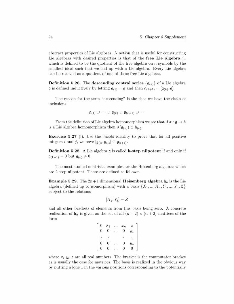
94 5. Chapter 5 Supplement
abstract properties of Lie algebras. A notion that is useful for constructingLie algebras with desired properties is that of the free Lie algebra fnwhich is defined to be the quotient of the free algebra on n symbols by thesmallest ideal such that we end up with a Lie algebra. Every Lie algebracan be realized as a quotient of one of these free Lie algebras.
Definition 5.26. The descending central series g(k) of a Lie algebrag is defined inductively by letting g(1) = g and then g(k+1) = [g(k), g].
The reason for the term “descending” is the that we have the chain ofinclusions
g(1) ⊃ · · · ⊃ g(k) ⊃ g(k+1) ⊃ · · ·
From the definition of Lie algebra homomorphism we see that if σ : g → h
is a Lie algebra homomorphism then σ(g(k)) ⊂ h(k).
Exercise 5.27 (!). Use the Jacobi identity to prove that for all positiveintegers i and j, we have [g(i), g(i)] ⊂ g(i+j).
Definition 5.28. A Lie algebra g is called k-step nilpotent if and only ifg(k+1) = 0 but g(k) 6= 0.
The most studied nontrivial examples are the Heisenberg algebras whichare 2-step nilpotent. These are defined as follows:
Example 5.29. The 2n+1 dimensional Heisenberg algebra hn is the Liealgebra (defined up to isomorphism) with a basis X1, ..., Xn, Y1, ..., Yn, Zsubject to the relations
[Xj , Yj ] = Z
and all other brackets of elements from this basis being zero. A concreterealization of hn is given as the set of all (n + 2) × (n + 2) matrices of theform
0 x1 ... xn z0 0 ... 0 y1...
......
...0 0 ... 0 yn
0 0 ... 0 0
where xi, yi, z are all real numbers. The bracket is the commutator bracketas is usually the case for matrices. The basis is realized in the obvious wayby putting a lone 1 in the various positions corresponding to the potentially
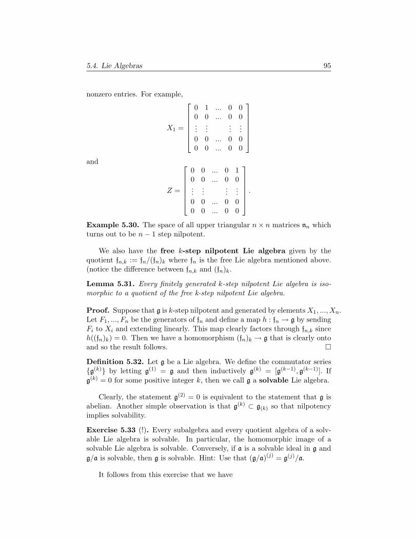
5.4. Lie Algebras 95
nonzero entries. For example,
X1 =
0 1 ... 0 00 0 ... 0 0...
......
...0 0 ... 0 00 0 ... 0 0
and
Z =
0 0 ... 0 10 0 ... 0 0...
......
...0 0 ... 0 00 0 ... 0 0
.
Example 5.30. The space of all upper triangular n× n matrices nn whichturns out to be n− 1 step nilpotent.
We also have the free k-step nilpotent Lie algebra given by thequotient fn,k := fn/(fn)k where fn is the free Lie algebra mentioned above.(notice the difference between fn,k and (fn)k.
Lemma 5.31. Every finitely generated k-step nilpotent Lie algebra is iso-morphic to a quotient of the free k-step nilpotent Lie algebra.
Proof. Suppose that g is k-step nilpotent and generated by elements X1, ..., Xn.Let F1, ..., Fn be the generators of fn and define a map h : fn → g by sendingFi to Xi and extending linearly. This map clearly factors through fn,k sinceh((fn)k) = 0. Then we have a homomorphism (fn)k → g that is clearly ontoand so the result follows. ¤
Definition 5.32. Let g be a Lie algebra. We define the commutator seriesg(k) by letting g(1) = g and then inductively g(k) = [g(k−1), g(k−1)]. Ifg(k) = 0 for some positive integer k, then we call g a solvable Lie algebra.
Clearly, the statement g(2) = 0 is equivalent to the statement that g isabelian. Another simple observation is that g(k) ⊂ g(k) so that nilpotencyimplies solvability.
Exercise 5.33 (!). Every subalgebra and every quotient algebra of a solv-able Lie algebra is solvable. In particular, the homomorphic image of asolvable Lie algebra is solvable. Conversely, if a is a solvable ideal in g andg/a is solvable, then g is solvable. Hint: Use that (g/a)(j) = g(j)/a.
It follows from this exercise that we have
96 5. Chapter 5 Supplement
Corollary 5.34. Let h : g → g be a Lie algebra homomorphism. Ifimg(h) := h(g) and ker(h) are both solvable then g is solvable. In par-ticular, if img(ad) := ad(g) is solvable then so is g.
Lemma 5.35. If a is a nilpotent ideal in g contained in the center z(g) andif g/a is nilpotent then g is nilpotent.
Proof. First, the reader can verify that (g/a)(j) = g(j)/a. Now if g/a isnilpotent then g(j)/a = 0 for some j and so g(j) ⊂ a and if this is the casethen we have g(j+1) = [g, g(j)] ⊂ [g, a] = 0. (Here we have [g, a] = 0 sincea ⊂ z(g).) Thus g is nilpotent. ¤
Trivially, the center z(g) of a Lie algebra a solvable ideal.
Corollary 5.36. Let h : g → g be a Lie algebra homomorphism. Ifim(ad) := ad(g) is nilpotent then g is nilpotent.
Proof. Just use the fact that ker(ad) = z(g). ¤Theorem 5.37. The sum of any family of solvable ideals in g is a solvableideal. Furthermore, there is a unique maximal solvable ideal that is the sumof all solvable ideals in g.
Sketch of proof. The proof is a maximality argument based on the follow-ing idea : If a and b are solvable then a∩ b is an ideal in the solvable a andso is solvable. It is easy to see that a + b is an ideal. We have by exercise5.13 (a + b)/b ∼= a/(a ∩ b). Since a/(a ∩ b) is a homomorphic image of a wesee that a/(a ∩ b)∼=(a + b)/b is solvable. Thus by our previous result a + b
is solvable. ¤Definition 5.38. The maximal solvable ideal in g whose existence is guar-anteed by the last theorem is called the radical of g and is denoted rad(g)
Definition 5.39. A Lie algebra g is called simple if it contains no idealsother than 0 and g. A Lie algebra g is called semisimple if it containsno abelian ideals (other than 0).Theorem 5.40 (Levi decomposition). Every Lie algebra is the semi-directsum of its radical and a semisimple Lie algebra.
The map ad : g →gl(g) = End(TeG) is given as the tangent map at theidentity of Ad which is a Lie algebra homomorphism. Thus by proposition?? we have obtain
Proposition 5.41. ad : g →gl(g) is a Lie algebra homomorphism.
Proof. This follows from our study of abstract Lie algebras and proposition??. ¤
5.4. Lie Algebras 97
Let’s look at what this means. Recall that the Lie bracket for gl(g) isjust A B −B A. Thus we have
ad([v, w]) = [ad(v), ad(w)] = ad(v) ad(w)− ad(w) ad(v)
which when applied to a third vector z gives
[[v, w], z] = [v, [w, z]]− [w, [v, z]]
which is just a version of the Jacobi identity. Also notice that using theantisymmetry of the bracket we get [z, [v, w]] = [w, [z, v]] + [v, [z, w]] whichin turn is the same as
ad(z)([v, w]) = [ad(z)v, w] + [v, ad(z)w]
so ad(z) is actually a derivation of the Lie algebra g as explained before.
Proposition 5.42. The Lie algebra Der(g) of all derivation of g is the Liealgebra of the group of automorphisms Aut(g). The image ad(g) ⊂ Der(g)is the Lie algebra of the set of all inner automorphisms Int(g).
ad(g) ⊂ Der(g)↓ ↓
Int(g) ⊂ Aut(g)
Let µ : G×G → G be the multiplication map. Recall that the tangentspace T(g,h)(G×G) is identified with TgG× ThG. Under this identificationwe have
T(g,h)µ(v, w) = ThLgw + TgRhv
where v ∈ TgG and w ∈ ThG. The following diagrams exhibit the relations:
G×G, (g, h)pr1 ‖
pr2G, g → G×G, (g, h) ← G,h
Rh
↓ µ Lg
G, gh
The horizontal maps are the insertions g 7→ (g, h) and h 7→ (g, h). Applyingthe tangent functor to the last diagram gives.
Tpr1 T(g,h)(G×G) Tpr2
l TgG → TgG× ThG ← ThG
↓ Tµ TgRh TghG ThLg
We will omit the proof but the reader should examine the diagrams and tryto construct a proof on that basis.
98 5. Chapter 5 Supplement
We have another pair of diagrams to consider. Let ν : G → G be theinversion map ν : g 7→ g−1. We have the following commutative diagrams:
Rg−1 (G, g) Lg−1
(G, e) ↓ ν (G, e)
Lg−1
(G, g−1
)Rg−1
Applying the tangent functor we get
TRg−1 TgG TLg−1
TeG ↓ Tν TeG
TLg−1 Tg−1G TRg−1
.
The result we wish to express here is that Tgν = TLg−1 TRg−1 = TRg−1 TLg−1 . Again the proof follows readily from the diagrams.
5.5. Geometry of figures in Euclidean space
We use differential forms in this section. We take as our first example thecase of a Euclidean space. We intend to study figures in En but we first needto set up some machinery using differential forms and moving frames. Lete1, e2, e3 be a moving frame on E3. Using the identification of TxE3 withR3 we may think of each ei as a function with values in R3. If x denotes theidentity map then we interpret dx as the map TE3 → R3 given by composingthe identity map on the tangent bundle TE3 with the canonical projectionmap TE3 = E3 × R3 → R3. If θ1, θ2, θ3 is the frame field dual to e1, e2, e3
then we may write
(5.3) dx =∑
eiθi.
Also, since we are interpreting each ei as an R3−valued function we maytake the componentwise exterior derivative to make sense of dei. Then dei
is a vector valued differential form: If ei = f1i + f2j + f3k then dei =df1i + df2j + df3k. We may write
(5.4) dej =∑
eiωij
5.5. Geometry of figures in Euclidean space 99
for some set of 1−forms ωij which we arrange in a matrix ω = (ωi
j). If wetake exterior derivative of equations 5.3 and 5.4 For the first one we calculate
0 = ddx =n∑
i=1
eiθi
=n∑
i=1
dei ∧ θi +n∑
i=1
ei ∧ dθi
=n∑
i=1
n∑
j=1
ejωij
∧ θi +
n∑
i=1
ei ∧ dθi.
From this we get the first of the following two structure equations. Thesecond one is obtained similarly from the result of differentiating 5.4.
dθi = −∑
ωij ∧ θj(5.5)
dωij = −
∑ωi
k ∧ ωkj
Furthermore, if we differentiate ei · ej = δij we find out that ωij = −ωj
i .If we make certain innocent identifications and conventions we can relate
the above structure equations to the group Euc(n) and its Lie algebra. Wewill identify En with the set of column vectors of the form
[1x
]where x ∈ Rn
Then the group Euc(n) is presented as the set of all square matrices of theform [
1 0v Q
]where Q ∈ O(n) and v ∈ Rn.
The action Euc(n)×En → En is then simply given by matrix multiplication(see chapter ??). One may easily check that the matrix Lie algebra that weidentify as the Lie algebra euc(n) of Euc(n) consists of all matrices of theform[
0 0v A
]where v ∈ Rn and A ∈ so(n) (antisymmetric matrices)
The isotropy of the point o :=[
10
]is easily seen to be the subgroup Go
consisting of all elements of the form[
1 00 Q
]where Q ∈ O(n)
which is clearly isomorphic to O(n). This isotropy group Go is just thegroup of rotations about the origin. The origin is not supposed to special
100 5. Chapter 5 Supplement
and so we should point out that any point would work fine for what we are
about to do. In fact, for any other point x ∼[
1x
]we have an isomorphism
Go∼= Gx given by h 7→ txhtx where
tx =[
1 0x I
].
(see exercise ??).For each x ∈ En tangent space TxEn consists of pairs x×v where v ∈ Rn
and so the dot product on Rn gives an obvious inner product on each TxEn:For two tangent vectors in TxEn, say vx = x × v and wx = x × w we have〈vx, wx〉 = v · w.
Remark 5.43. The existence of an inner product in each tangent spacemakes En a Riemannian manifold (a smoothness condition is also needed).Riemannian geometry (studied in chapter ??) is one possible generalizationof Euclidean geometry (See figure 17 and the attendant discussion). Rie-mannian geometry represents an approach to geometry that is initially quitedifferent in spirit from Klein’s approach.
Now think of each element of the frame e1, ..., en as a column vector offunctions and form a matrix of functions e. Let x denote the “identity map”given as a column vector of functions x = (x1, x2, x3) = (x, y, z). Next weform the matrix of functions [
1 0x e
]
This just an element of Euc(n)! Now we can see that the elements of Euc(n)are in a natural 1 − 1 correspondents with the set of all frames on En andthe matrix we have just introduce corresponds exactly to the moving framex 7→ (e1(x), ..., en(x)). The differential of this matrix gives a matrix of oneforms
$ =[
0 0θ ω
]
and it is not hard to see that θ is the column consisting of the same θi as
before and also that ω = (ωij). Also, notice that x 7→ $(x) =
[0 0θ ω
]
takes values in the Lie algebra euc(n). This looking like a very natural stateof affairs. In fact, the structure equations are encoded as a singe matrixequation
d$ = $ ∧$.
The next amazingly cool fact it that if we pull-back $ to Euc(n) via
the projection π :[
0 0x e
]7→ x ∈ En then we obtain the Maurer-Cartan

5.5. Geometry of figures in Euclidean space 101
form of the group Euc(n) and the equation d$ = $ ∧$ pulls back to thestructure equations for Euc(n).

Chapter 6
Chapter 6 Supplement
6.1. Comments and Errata
6.1.1. Comments. In the definition of structure groups for fibers bundleswe cosidered only the case that the action is effective. Then since the cor-responding homomorphism G → Diff(F ) given by g 7→ λg is injective, thereader may feel that the group G can be replaced by its image in Diff(F ). In-deed, by transferring the Lie group structure by brute force onto this image,one may indeed replace G by its image. However, it is not always desirablenor convenient to do so.
6.1.2. Errata. (Nothing yet)
6.2. sections of the Mobius band
Consider the C0-vector bundle obtained in the following way. Start with thefirst factor projection [0, 1]×R→ [0, 1]. On [0, 1]×R define the equivalencerelation (0, a) ∼ (1,−a) and let Mb = ([0, 1]× R) /∼ with the quotienttopology. On [0, 1], define an equivalence relation by identifying 0 with 1.Then [0, 1]/∼ is identified with S1. The first factor projection induces acontinuous map
π : Mb → S1
which is easily seen to be a vector bundle of rank 1. In the category of generalcontinuous bundles over S1, this bundle is equivalent to the Mobius bandbundle introduced in the main text. This bundle can be given a smoothvector bundle structure quite easily, but we only need the C0 version tomake our point about global nonzero sections. This is the vector bundleversion of the Mobius band and is also referred to by the same name. By
103
104 6. Chapter 6 Supplement
considering the quotient construction used to obtain π : Mb → S1 we seethat a global continuous section σ of π : Mb → S1 must correspond, underthe quotient, to a continuous map σ : [0, 1] → R such that σ(0) = −σ(1).By continuity, such a map must be zero at some point which forces σ to bezero also. Thus π : Mb → S1 is not trivial.
6.3. Etale space of a sheaf
Let E → M be a vector bundle and consider the sheal for local sections.Recall that s1 ∈ ΓE(U) and s2 ∈ ΓE(V ) determine the same germ of sectionsat p if there is an open set W ⊂ U ∩ V such that rU
W s1 = rVW s2. We impose
an equivalence relation on the union⋃
p∈U
ΓE(U)
by declaring that s1 ∼ s2 if and only if s1 and s2 determine the same germof sections at p. The set of equivalence classes (called germs of sections at p)is an abelian group in the obvious way and is denoted ΓE
p . If we are dealingwith a sheaf of rings, then ΓE
p is a ring. The set ΓE((U)) :=⋃
p∈U ΓEp is
called the sheaf of germs and can be given a topology so that the projection
pr : ΓE((U)) → M ,
defined by the requirement that pr([s]) = p if [s] ∈ SEp , is a local homeo-
morphism. The idea generalizes:
Definition 6.1. Mp is a set of equivalence classes called germs at p. Heres1 ∈ M(U) and s2 ∈ M(V ) determine the same germ of sections at p ifthere is an open set W ⊂ U ∩ V containing p such that rU
W s1 = rVW s2. The
germ of s ∈M(U) at p is denoted sp.
Now we form the union M =⋃
p∈M Mp and define a surjection π : M →M by the requirement that π(sp) = p for sp ∈ Mp. The space M is calledthe sheaf of germs generated by M. We want to topologize M so that πis continuous and a local homeomorphism, but first we need a definition:
Definition 6.2 (etale space). A topological space Y together with a con-tinuous surjection π : Y → M that is a local homeomorphism is called anetale space. A local section of an etale space over an open subset U ⊂ Mis a map sU : U → Y such that π sU = idU . The set of all such sectionsover U is denoted Γ(U, Y ).
Definition 6.3. For each s ∈M(U), we can define a map (of sets) s : U →M by
s(x) = sx
6.4. Discussion on G bundle structure 105
and we give M the smallest topology such that the images s(U) for allpossible U and s are open subsets of M.
With the above topology M becomes an etale space and all the sectionss are continuous open maps. If we let M(U) denote the sections over U
for this etale space, then the assignment U → M(U) is a presheaf that isalways a sheaf. We give the following without proof:
Proposition 6.4. If M is a sheaf, then M is isomorphic as a sheaf to M.
6.4. Discussion on G bundle structure
It is well understood that one starting point for defining a G-bundle struc-ture on a locally trivial fibration is the idea that a G-bundle structure isdetermined by a bundle atlas that in some sense takes values in a Lie groupor topological group G. This is similar to the idea that a C∞-atlas deter-mines a smooth structure on a locally Euclidean paracompact topologicalspace. But when do two G-bundle atlases determine the very same G-bundlestructure? There are several ways one may describe the situation but wewill show that one way which occurs in the literature is actually wrong.This wrong way actually describes a special case of a different equivalencerelation that says when two different G-bundles are equivalent but not nec-essarily the same. It does not reduce to the correct notion in this specialcase. This is analogous to the notion of two different smooth structureson a fixed topological manifold being nevertheless diffeomorphic. One doesnot want to confuse the notion of diffeomorphism class with the notion ofa smooth structure. One would also like to avoid a similar confusion in thedefinition and classification of G-bundles. That is we do not want to con-fuse G-bundle structures with the notion of equivalence classes of G-bundlestructures (even on a single fibration).
The bottom line will be that Steenrod got it right in his famous book”The topology of fiber bundles”. The key overlooked notion is that of strictequivalence defined on page 8 of the 1999 Princeton edition. Strict equiv-alence is to be contrasted with the second important notion of equivalencementioned above that is cohomological in nature. There are several placesin the literature, including textbooks, where the notion of strict equivalenceis conflated with the weaker cohomological notion. We shall convince thereader that these are importantly different and have different roles and donot coincide even if one is dealing with a single fibration (fixed total spaceand base space).
6.4.1. Two notions of equivalence. For concreteness let us work in thesmooth category. Let π : E → M be a locally trivial fibration with typical
106 6. Chapter 6 Supplement
fiber F . Suppose that ρ : G× F → F is an appropriately smooth action ofa Lie group G on F so that G acts by diffeomorphisms of F . (We will thinkin terms of actions rather than representations).
Recall that each bundle chart (ϕα, Uα) gives a diffeomorphism ϕα,x :Ex → F for each x ∈ Uα. Notice that each ϕα must have the form ϕα =(π, Φα) for some smooth map Φα : π−1(Uα) → F . Then ϕα,x := Φα|Ex
. If(ϕα, Uα) and (ϕβ, Uβ) are bundle charts for π : E → M , then the ”raw”transition functions (between the charts) are defined by
ϕαβ(x) := ϕα,x ϕ−1β,x
and for each x ∈ Uα ∩ Uβ, the map ϕαβ(x) : F → F is a diffeomorphism ofF .
Definition 6.5. A (G, ρ)-atlas consists of a cover of the bundle by localtrivializations or bundle charts (ϕα, Uα) such that there exist smooth mapsgαβ : Uα ∩ Uβ → G defined whenever Uα ∩ Uβ 6= ∅, such that
ϕαβ(x)(y) = ρ(gαβ(x), y) for y ∈ F .
We further require that the family gαβ satisfy the cocycle conditions
gαα(p) = e for p ∈ Uα
gαβ(p) = (gβα(p))−1 for p ∈ Uα ∩ Uβ
gαβ(p)gβγ(p)gγα(p) = e for p ∈ Uα ∩ Uβ ∩ Uγ
Notice that the cocycle condition would be automatic if the action ρ :G × F → F were assumed to be an effective action. Otherwise the cocyclecondition is necessary to keep contact with the important notions of principalbundle and associated bundle which are the basic notions in an alternativedevelopment of G-bundles (which seems to be due to Ehresmann). Alsonotice that for an ineffective action, the functions ϕαβ(x) do not uniquelydetermine the G-valued functions gαβ(x)! Thus if we do not restrict ourselvesto effective actions (as does Steenrod) we must actually include the thecocycle as part of the data. Thus we must specify
Data := (E, π, M, F,G, ρ, (ϕα, Uα)α∈A , gαβ).Indeed, it may be the case that there is another quite different cocycle g′αβsuch that ϕαβ(x)(y) = ρ(g′αβ(x), y) for all x ∈ Uα ∩Uβ and y ∈ F . One only
needs to have gαβ(x)(g′αβ(x)
)−1in the kernel of the action for each x. This
causes all the definitions to be far more complicated in many places thanthose found in Steenrod since he restricts himself to effective actions. Thisis true even for the notion of strict equivalence that we wish to explore next.
So as to not obscure the main issue let us restrict ourselveseffective actions.
6.4. Discussion on G bundle structure 107
We now come to the main question:
When do two (G, ρ)-atlases define the same (G, ρ)-bundle structure?
This is a question of how to make an appropriate definition. We canphrase the question by asking when the data
Data1 := (E, π,M,F, G, ρ, (ϕα, Uα)α∈A)
is appropriately equivalent to similar data
Data2 := (E, π, M, , F,G, ρ, (ψj , Vj)j∈J ).
The most straightforward notion of equivalence for this purpose is the fol-lowing
Definition 6.6 (strict equivalence). Let ρ be effective. If (ϕα, Uα)α∈A and(ψj , Vj)j∈J are both (G, ρ)-atlases on a bundle (E, π, M) then (ϕα, Uα)α∈A
is strictly equivalent to (ψj , Vj)j∈J if (ϕα, Uα)α∈A
⋃ (ψj , Vj)j∈J isa (G, ρ)-atlas (with new larger and uniquely determined cocycle since ρ iseffective).
This is equivalent to Steenrod’s definition:
Definition 6.7 (strict equivalence 2). Let ρ be effective. If (ϕα, Uα)α∈A
and (ψj , Vj)j∈J are both (G, ρ)-atlases on a bundle (E, π,M) then (ϕα, Uα)α∈A
is strictly equivalent to (ψj , Vj)j∈J if for each α ∈ A and j ∈ J suchthat Uα ∩ Uβ 6= ∅ we have that there are smooth maps gαj : Uα ∩ Vj → Gand gjα : Uα ∩ Vj → G such that
ϕα,x ψ−1j,x(y) = ρ(gαj(x), y)
ψj,x ϕ−1α,x(y) = ρ(gjα(x), y)
for all x ∈ Uα ∩ Vj and y ∈ F .
It is not hard to show that the above two definitions are equivalent andwe can define a (G, ρ)-bundle structure to be a strict equivalence class of(G, ρ)-atlases.
Definition 6.8. A (G, ρ)-bundle structure is a strict equivalence class of(G, ρ)-atlases.
Now consider the following notion of equivalence, which we claim isweaker:
108 6. Chapter 6 Supplement
Definition 6.9. Let ρ be effective. If (ϕα, Uα)α∈A and (ψj , Vj)j∈J areboth (G, ρ)-atlases on a bundle (E, π, M) then (ϕα, Uα)α∈A is equiva-lent2 to (ψj , Vj)j∈J if there are smooth maps gjα : Uα ∩ Vj → G andgαj : Uα ∩ Vj → G for each α ∈ A and j ∈ J such that
gjα(x) = gjβ(x)gβα(x) for all x ∈ Uα ∩ Uβ ∩ Vj
glα(x) = g′lk(x)gkα(x) for all x ∈ Uα ∩ Vk ∩ Vl
and similarly for gαj . Here gβα(x) and g′lk(x) are the cocycles uniquelydetermined by (ϕα, Uα)α∈A and (ψj , Vj)j∈J respectively (notice thatwe need effectiveness of the action here!)
This definition is a bit cumbersome and tough to think about, but no-tice that the sets of the form Uα ∩ Vj cover M and form a refinementof both Uαand Vj so that (ϕα, Uα)α∈A and (ψj , Vj)j∈J are eachstrictly equivalent to atlases with the same cover (but not necessarilystrictly equivalent to each other as we shall see). Call these atlases(ϕi, Ui)i∈I and (ψi, Ui)i∈I and notice that we have a new indexing set Iand we have renamed the cover for simplicity.
It is not hard to show that the following is an alternative characterizationof equivalence2 in this case.
Definition 6.10. Let ρ be effective. If (ϕi, Ui)i∈I and (ψi, Ui)i∈I areboth (G, ρ)-atlases on a bundle (E, π,M) then (ϕi, Ui)i∈I is equivalent2
to (ψj , Uj)j∈J if and only if there exist smooth functions λi : Ui → G suchthat
g′ji(x) = λj(x)−1gji(x)λi(x) for all x ∈ Ui ∩ Uj
We say that (ϕi, Ui)i∈I and (ψi, Ui)i∈I give rise to cohomologous co-cycles.
Now we come to our first main assertion:
If (ϕi, Ui)i∈I and (ψi, Ui)i∈I are strictly equivalent then they areequivalent2 but the converse is not necessarily true.
The fact that strict equivalence implies the weaker equivalence is aneasy exercise. The fact the converse is not true becomes apparent alreadyfor trivial bundles and even bundles over a single point.
Example 6.11. Let us consider the case of a Gl(n) structure on a bundleover a zero dimensional manifold. Thus we are essentially working witha single fiber X. The Gl(n) structure on X is certainly supposed to bea vector space structure. Indeed, if we have a family of diffeomorphismsϕi : X → Rni∈I such that ϕιj := ϕi ϕ−1
j is in Gl(n) for every i, j then wehave a Gl(n)-atlas and we get a well defined vector space structure on X.
6.4. Discussion on G bundle structure 109
(In fact all we need is one such chart.) Clearly two families of maps that arestrictly equivalent will give the same vector space structure. Indeed, strictequivalence of ψi and ϕi would just mean that ϕi ψ−1
j is always inGl(n) for all i, j ∈ I.But now let h : X → X be any randomly chosen diffeomorphism1 and letψi : X → Rni∈I be defined by ψi := ϕi h. Then
g′ij := ψi ψ−1j = (ϕi h) (ϕj h)−1
= ϕi h h−1 ϕ−1j = ϕi ϕ−1
j = gij
so not only does ψi give rise to a cocycle cohomologous to that of ϕi,it gives rise to the very same cocycle! But we certainly don’t expect ψiand ϕi to give the same vector space structure on X since h was chosenarbitrarily.
Notice that due to the arbitrary nature of h, the cohomologous equiva-lence is essentially vacuous in this case. This is as it should be since we areworking over a point and the same would be true over a contractible basespace. On the other hand, the strict equivalence defines the ”geometrically”significant notion of vector space structure on X. If one tried to use thesecond weaker notion of equivalence then we wouldn’t end up with a vectorspace structure–we wouldn’t even have a consistent way of adding elementsof X.
Remark 6.12. If we were to compare atlases ϕi and ψi = f ϕi wheref : Rn → Rn is a linear isomorphism then we would have cohomologous, butin this case, also strictly equivalence atlases. If f is only assumed to be adiffemorphism then g′ij = f ϕi ϕ−1
j f−1 = f gij f−1 is not necessarilylinear so the atlas ψi = f ϕi is not even a Gl(n)-atlas at all.
The example above, can be generalized to bundles over disks and thenwe see that using the wrong notion of equivalence would result in a falsenotion of Gl(n)-bundle structure that would leave us without a well definedmodule structure on the space of sections of the bundle–the fibers don’t evenbecome vector spaces.
It is often said that an O(n) structure on vector bundle is just a choiceof metric tensor. If the bundle has only one fiber again then this is just aquestion of when one can use these maps to define an inner product structureon a set X.
1We are in the smooth category but it is the only bijective nature of the map that will beused.
110 6. Chapter 6 Supplement
Example 6.13. Let us consider the case of a O(n) structure on a bundleover zero dimensional manifold. Thus we are essentially working with a sin-gle fiber X. The O(n)-bundle structure on X is certainly supposed to be aan inner product space structure. Indeed, if we have a family of diffeomor-phisms ϕi : X → Rni∈I such that ϕij := ϕi ϕ−1
j is in O(n) for every i, jthen we have well defined vector space structure on X and an inner productcan be defined by
〈x, y〉 := ϕ−1i (x) · ϕ−1
i (y) (dot product)
and this is independent of i. Clearly, two such family of maps that are strictlyequivalent, will give the same inner product space structure. Indeed, strictequivalence of ψi and ϕi would just mean that ϕi ψ−1
j is always inO(n).But now let h : X → X be any randomly chosen diffeomorphism and letψi : X → Rni∈I be defined by ψi := ϕi h. Then
g′ij := ψi ψ−1j = (ϕi h) (ϕj h)−1
= ϕi h h−1 ϕ−1j = ϕi ϕ−1
j = gij .
So, not only does ψi give rise to a cocycle cohomologous to that of ϕi,it gives rise to the very same cocycle! But we certainly don’t expect ψiand ϕi to give the same inner product structure on X since h was chosenarbitrarily.
Example 6.14. Let D be the 2-disk (x, y, 0) ∈ R3 : x2 + y2 < 1. Givethis manifold the flat metric it inherits from R3. This gives the tangentbundle TD an O(2)-bundle structure which is the same one that we get ifwe use the single vector bundle chart (ϕ,D) coming from the standard o.n.frame field on D. But now consider the projection of the upper hemisphereS2
+ onto D. Use this to transfer an orthonormal frame from the curvedspace S2
+ to D. This puts a different metric on D which now has curvaturew.r.t the associated Levi-Civita connection. This is the same O(2)-bundlestructure that we get if we use the single vector bundle chart (ψ, D) comingfrom this new frame field on D. But while the O(2)-atlas (ϕ,D) is notstrictly equivalent to (ψ, D), it is equivalent in the cohomologous senseby an argument formally the same as the one in the last example. Wecertainly do not want to say that they define the very same O(n)-bundlestructure. Indeed, they are two different metrics. Here we see that theO(2)-bundle structure itself can have a rigid geometric significance whilethe weaker cohomological notion retains a mainly topological significance.
6.4. Discussion on G bundle structure 111
The point is that one needs to first define a G-bundle structure using thenotion of strict equivalence and then talk about when two such structures(possibly on the very same fibation) are equivalent.
6.4.2. Explanation. The notion of strict equivalence for G-atlases (witheffective action) is used to define a G-bundle structure on a bundle. Itis analogous to the equivalence of atlases for smooth manifolds where twosuch are equivalent if they are both subsets of the maximal atlas. Thecohomological equivalence which we have called equivalence2 is a specialcase of equivalence of two different G-bundles, where in this case, we justhappen to have the same underlying fibration. It is similar to having twoatlases which induce two different smooth structures on the same topologicalmanifold which may nevertheless be diffeomorphic structures.
Let us put the weaker notion of equivalence in its proper context. Inthe general case, one considers two different total spaces and then the coho-mologous cycle equivalence is the same as the following notion of G-bundleequivalence:
Definition 6.15. Let ξ1 = (E1, π1,M1, F ) be a (G, ρ)-bundle with its (G, ρ)-bundle structure determined by the strict equivalence class of the (G, ρ)-atlas(ϕα, Uα)α∈A. Let ξ2 = (E2, π2,M2, F ) be a (G, ρ)-bundle with its (G, ρ)-bundle structure determined by the strict equivalence class of the (G, ρ)-atlas(ψβ, Vβ)β∈B. Then a bundle morphism (h, h) : ξ1 → ξ2 is called a (G, ρ)-bundle morphism along h : M1 → M2 ifi) h carries each fiber of E1 diffeomorphically onto the corresponding fiberof E2;ii) whenever Uα ∩ h−1 (Vβ) is not empty, there is a smooth map hαβ : Uα ∩h−1 (Vβ) → G such that for each p ∈ Uα ∩ h−1 (Vβ) we have
(Ψβ h
(Φα|π−1
1 (p)
)−1)
(y) = ρ(hαβ(p), y) for all y ∈ F ,
where as usual ϕα = (π1, Φα) and ψβ = (π2,Ψβ). If M1 = M2 and h = idM
then we call h a (G, ρ)-bundle equivalence over M . (In this case, h is adiffeomorphism).
For this definition to be good it must be shown to be well defined.That is, one must show that condition (iii) is independent of the choiceof representatives (ϕα, Uα)α∈A and (ϕi, Vi)i∈J of the strict equivalenceclasses of atlases on the repsective bundles.
Now we see that the notion we have called ”equivalence2” is just theassertion that two different (G, ρ)-bundle structures on the very same fibra-tion are (G, ρ)-bundle equivalent. We have also seen that equivalence2 is notwhat should be used to define (G, ρ)-bundle structure in the first place.
112 6. Chapter 6 Supplement
Finally, we comment that one can approach (G, ρ)-bundle structuresvia principal bundles which can be defined without recourse to equivalenceclasses of bundle atlases. One must specify the right action since a singlespace can have more than one right action. In this case, we may have twodifferent principal bundles (P, π, M, G, r1) and (P, π, M, G, r2) which differonly in the right action while the spaces are the same. Then (P, π, M, G, r1)is equivalent to (P, π,M,G, r2) if there is a fiber preserving map P → Pthat is also a G-map. This corresponds to equivalence2 while equivalence1 isnow unnecessary since the principal G-bundle is now our starting point. Insome sense the principal bundle just is the G-bundle structure for itself andall its associated vector bundles. (More on this to come). In fact, a G-cocyleis just what one needs to construct a principal G-bundle in the case whereall one knows is information about overlaps for some atlas of fiber bundlelocal trivializations. Alternatively, in the case of vector bundles where ρcan be taken as a representation of G on the typical fiber V , then we canthink of a vector bundle E → M as having a (G, ρ)-bundle structure ifthere is a principal G-bundle P and a bundle map f : P → F (E) such thatf(ug) = f(u) ρ(g).
Remark 6.16. (G-bundle structures vs. “G-bundle structures”) We havedeliberately opted to use the term “G-bundle structure” rather that simply“G-structure” which could reasonably be taken to mean the same thing.Perhaps the reader is aware that there is a theory of G-structures on asmooth manifold (see ). One may rightly ask whether a G-structure on Mis nothing more than a G-bundle structure on the tangent bundle TM whereG is a Lie subgroup of GL(n) acting in the standard way. The answer isboth yes and no. First, one could indeed say that a G-structure on M is akind of G-bundle structure on TM even though the theory is usually fleshedout in terms of the frame bundle of M (defined below). However, the notionof equivalence of two G-structure on M is different than what we have givenabove. Roughly, G-structures on M are equivalent in this sense if there is adiffeomorphism φ such that (Tφ, φ) is a type II bundle isomorphism that isalso a G-bundle morphism along φ.
6.4.3. Effectiveness of the Action. We wish to make some commentson the fact that we have chosen to assume the action ρ is effective. Let usreturn to the ”coordinate bundle” viewpoint again and consider the taskof developing good definitions without the effectivelness assumption. Thisis the assumption made in Steenrod’s book on page 7. He keeps this as-sumption throughout and so for Steenrod, the structure group of the bundle∧kTM cannot be taken to be Gl(n) since the latter acts ineffectively on∧kRn Without the assumption of an effective action, we must include the
6.4. Discussion on G bundle structure 113
cocyle as part of the data. Indeed, the equations
ϕαβ(x)(y) = ρ(gαβ(x), y) for y ∈ F
used in the definition do not determine the gαβ and they may only satisfythe cocyle conditions modulo the kernel of the action! This is actually aserious problem.
Remark 6.17. On page 63 of the 3rd edition Husemoller’s book we findthe following sentence:“Properties (T1) to (T2) [cocycle conditions] follow from the fact that gi,j
is the only map satisfying the relation hj(b, y) = hi(b, gi,j(b)y).”The statement only makes sense if G acts effectively. But Husemoller hasnot made such an assumption prior to this nor after this statement. Muchof what follows needs the effectiveness and yet many of the actions he usesare not effective (consider how the bundle
∧kTM is an associated bundlefor the frame bundle via an ineffective action
∧kρ0 where ρ0 is the standardaction of Gl(n) on Rn. Not that the way Steenrod would contruct a tensorbundle is by starting with a homomorphism h : Gl(n) → G where G actseffectively on
∧kRn and G is the structure group (See section 6.3 on page 21of Steenrod). Steenrod takes a Gl(n)−valued cocyle and composed with h toobtain a G-valued cocyle and only then does he use the bundle constructiontheorem to obtain a G-bundle. In the associated bundle construction aspresented in Husemoller’s book, one would use the ineffective representationρ : Gl(n) → Gl(
∧kRn) and form the associated bundle
F (M)×ρ∧kRn.
One is then tempted to say that Gl(n) is the structure group or that ρ isthe ineffective structure representation. To get more in line with Steenrodone should quotient both ρ and the frame bundle by K = ker ρ and onlythen produce an associated bundle. The quotiented frame bundle would bya Gl(n)/K bundle where Gl(n)/K isomorphic to G.
So, if we wish to proceed using atlases a la Steenrod, how shall we define(G, ρ)-structure in case ρ is ineffective? At the very least we must assumethat each atlas is associated to a true G-cocyle and not just a cocyle modulothe kernel of the action (A G-principal bundle must be lurking) . Lessonsfrom the theory of spin structures show that this is a nontrivial assumption.Second; how shall we formulate a notion of strict equivalence? If we simplytake the union of two (G, ρ)-atlases then we may not end up with an atlasthat is a associated to a larger inclusive G-cocyle (one again we only get thecocycle conditions up to the kernal of ρ). So we must just assume that thecombined (G, ρ)-atlas comes with a cocycle. Can we obtain a maximal suchatlas with a single maximal canonical cocyle?
114 6. Chapter 6 Supplement
The authors hope that the final version of this note will be able tosort this out by taking clues from the theory of principal and associatedbundles. But, so far, it has proved rather slippery; there always seems to bea defeating loop hole that traces back to the ineffectiveness issue.
Chapter 8
Chapter 8 Supplement
8.1. Comments and Errata
8.1.1. Comments. The exterior derivative is indeed special. It was provedby R. Palais that if D : Ω(M) → Ω(M) is a map defined for all smoothmanifolds such that D(Ωk(M)) ⊂ Ω`(M) and such that for every smoothmap f : M → N the diagram below commutes,
Ωk(N)f∗→ Ωk(M)
D ↓ ↓ D
Ω`(N)f∗→ Ω`(M)
then one of the following holds:
(1) D = 0,
(2) D is a multiple of the identity map (so k = `),
(3) D is a multiple of exterior differentiation or k = dim M , ` = 0 andD is a multiple of integration as defined and studied in the nextchapter.
8.1.2. Errata. (Nothing yet)
8.2. 2-Forms over a surface in Euclidean Space Examples.
We just parametrize the surface as r(u, v) = (x(u, v), y(u, v), z(u, v)) forsome region of u, v. Let
ω = F1(x, y, z)dy ∧ dz + F2(x, y, z)dz ∧ dx + F3(x, y, z)dx ∧ dy
115
116 8. Chapter 8 Supplement
be our 2-form. Then dy = ∂y∂udu + ∂y
∂vdv and dz = ∂z∂udu + ∂z
∂vdv so
dy ∧ dz =(
∂y
∂udu +
∂y
∂vdv
)∧
(∂z
∂udu +
∂z
∂vdv
)
=∂y
∂u
∂z
∂vdu ∧ dv +
∂y
∂v
∂z
∂udv ∧ du
=∂y
∂u
∂z
∂vdu ∧ dv − ∂y
∂v
∂z
∂udv ∧ du
=(
∂y
∂u
∂z
∂v− ∂y
∂v
∂z
∂u
)du ∧ dv
=
∣∣∣∣∣∂y∂u
∂y∂v
∂z∂u
∂z∂v
∣∣∣∣∣ du ∧ dv =∂(y, z)∂(u, v)
du ∧ dv
(only involves u and v)
We have seen that before! Likewise we figure out dz ∧ dx and dx ∧ dy interms of u and v. So we get
∫ω =
∫F1(x, y, z)dy ∧ dz + F2(x, y, z)dz ∧ dx + F3(x, y, z)dx ∧ dy
=∫ ∫ (
F1∂(y, z)∂(u, v)
+ F2∂(z, x)∂(u, v)
+ F3∂(x, y)∂(u, v)
)dudv
=∫ ∫
〈F1, F2, F3〉 · (ru × rv) du dv =∫∫S
F · n dS
So∫
ω =∫∫S
F ·n dS as long as we use the correspondence F ¿ ω or in detail
F1(x, y, z)i + F2(x, y, z)j + F3(x, y, z)k ¿ F1(x, y, z)dy ∧ dz + F2(x, y, z)dz ∧ dx + F3(x, y, z)dx ∧ dy
Example 8.1. Let ω = xdy∧dz and consider the surface which is the graphof z = 1 − x − y where x and y only vary over the region 0 ≤ x ≤ 1 and0 ≤ y ≤ 1− x. Then we can use x and y as our parameters. So
∂(y, z)∂(x, y)
=(
∂y
∂x
∂z
∂y− ∂y
∂y
∂z
∂x
)
= 0− ∂z
∂x= 1
∫ω =
∫xdy ∧ dz
=∫ 1
0
∫ 1
0
(x
∂(y, z)∂(x, y)
)dxdy
=∫ 1
0
(∫ 1−x
0xdy
)dx =
16
8.3. Pseudo-Forms 117
Example 8.2. Let ω = xdy ∧ dz and consider the hemisphere S+ of radius1 centered ot the origin. This is parameterized by
r(φ, θ) = (x(φ, θ), y(φ, θ), z(φ, θ))
= (sinφ cos θ, sinφ sin θ, cosφ)
with 0 ≤ θ ≤ 2π and 0 ≤ φ ≤ π/2. Then dy = ∂y∂φdφ + ∂y
∂θdθ and dz =∂z∂φdφ + ∂z
∂θdθ or
dy = cosφ sin θ dφ + sinφ cos θ dθ
dz = − sinφdφ + 0 dθ
so
ydy ∧ dz = (sinφ cos θ) (cos φ sin θ dφ + sin φ cos θ dθ) ∧ (− sinφdφ)
= − sin2 φ sin θ cos2 θ dθ ∧ dφ = sin2 φ sin θ cos2 θ dφ ∧ dθ
Thus ∫
S+
ω =∫ π
0
∫ π/2
0sin2 φ sin θ cos2 θ dφdθ =
16π
8.3. Pseudo-Forms
Let M be a smooth n-manifold. Recall that the set of frames e1, ..., en inTpM are divided into two equivalence classes called orientations. Equiva-lently, an orientation at p is an equivalence class of elements of ∧nT ∗p M . Foreach p there are exactly two such orientations and the set of all orientationsor(M) at all points p ∈ M form a set with a differentiable structure andthe map πor that takes both orientations at p to the point p is a two foldcovering map. Rather than a covering space what we would like at this pointis a rank one vector bundle. We now construct the needed bundle with iscalled the flat orientation line bundle and denoted Oflat(TM). Sectionsof Oflat(TM) are sometimes called pseudoscalar fields. For each p ∈ M weconstruct a one dimensional vector space Op. Let
Sp = (p, µp, a) : a ∈ R, [µp] an orientation on TpMThus µp is one of the two orientations of TpM . The define an equivalencerelation on Sp by declaring that (p, [µp] , a) is equivalent to (p, [−µp] ,−a).Denote the equivalence class of (p, [µp] , a) by [p, [µp] , a]. Then we let Op :=Sp/ ∼. The set Op has a one dimensional vector space structure such that
[p, [µp] , a] + [p, [µp] , b] = [p, [µp] , a + b]
r[p, [µp] , a] = [p, [µp] , ra]
for a, b, r ∈ R. Now let
Oflat(TM) :=⋃
p∈M
Op .
118 8. Chapter 8 Supplement
We have the obvious projection π : Oflat(TM) → M given by [p, [µp] , a] 7→ p.An atlas (Uα, xα) for M induces a vector bundle atlas for Oflat(TM) asfollows: For a chart (Uα, xα) define
ψα : π−1(Uα) → Uα × Rby ψα([p, [µp] , a]) = (p, εa) where ε = 1 or −1 according to whether Tpψα :(TpM, [µp]) → Rn is orientation preserving or not. Associated with such achart we have the local section
oxα : p 7→ [p, [µp (xα)] , a]
where µp (xα) = dx1 ∧ · · · ∧ dxn. In fact, if U is any orientable open set inM with orientation given by [µ] where µ ∈ Ωn(U) then we can regard [µ] asa local section of Oflat(TM) as follows:
[µ] : p 7→ [p, [µ(p)] , 1]
With this this VB-atals the transition functions gαβ : Uα∩Uβ → Gl(1,R)defined by
gαβ(p) :=det
(Txα Tx−1
β
)∣∣∣det
(Txα Tx−1
β
)∣∣∣= ±1
and so we see that we have a structure group O(1). Thus the transitionfunctions are locally constant (which is why we call this bundle flat).
A pseudo-k-form (or twisted k-form ) is a cross section of Oflat(TM) ⊗∧kT ∗M . The set of all twisted k-forms will be denoted by Ωk
o(M). Sectionsof Ωk
o(M) can be written locally as sums of elements of the form o⊗θ whereo is an orientation of U regarded as a local section of Oflat(TM) as describedabove. Now we can extend the exterior product to maps
∧ : Ωko(M)× Ωl(M) → Ωk+l
o (M)
by the rule (o1 ⊗ θ1) ∧ θ2 = o1 ⊗ θ1 ∧ θ2 with a similar and obvious map∧ : Ωk(M)× Ωl
o(M) → Ωk+lo (M). Similarly, we have a map ∧ : Ωk
o(M)×Ωl
o(M) → Ωk+l(M) given by
(o1 ⊗ θ1) ∧ (o2 ⊗ θ2) = (o1o2) θ1 ∧ θ2
and where (o1o2) is equal to +1 wherever o1 = o2 and −1 otherwise. Now wecan extend the exterior algebra to
∑nk,l=0
(Ωk(M)⊕ Ωl
o(M)). If ω ∈ Ωk
o(M)then with respect to the chart (Uα, xα), ω has the local expression
ω = oxα ⊗ aα~Idx
~Iα
8.3. Pseudo-Forms 119
and if ω = oxβ⊗ aβ
~Jdx
~Jβ for some other chart (Uβ, xβ) then
aα~I
=det
(xα x−1
β
)∣∣∣det
(xα x−1
β
)∣∣∣∂x
~Jα
∂x~Iβ
aβ~J
In particular if ω is a pseudo n-form (a volume pseudo-form) where n =
dimM , then ~I = (1, 2, ..., n) = ~J and ∂x~Jα
∂x~Iβ
= det(xα x−1
β
)and so the rule
becomes
aα12..n =
det(xα x−1
β
)∣∣∣det
(xα x−1
β
)∣∣∣det
(xα x−1
β
)aβ
12..n
oraα
12..n =∣∣∣det
(xα x−1
β
)∣∣∣ aβ12..n.
There is another way to think about pseudo forms that has the advantageof having a clearer global description. The group Z/2Z =1,−1 acts as decktransformations on or(M) so that −1 sends each orientation to its opposite.Denote the action of g ∈ Z/2Z by lg : or(M) → or(M). Now we think ofa pseudo k-form as being nothing more than a k-form η on the manifoldor(M) with the property that l∗−1η = −η. Now we would like to be able tointegrate a k-form over a map h : N → M where N is a k-manifold. Bydefinition h is orientable if there is a lift h : or(N) → or(M)
or(N) h→ or(M)↓ πOrN
↓ πOrM
Nh→ M
We will say that h is said to orient the map. In this case we define theintegral of a pseudo k-form η over h to be∫
hη :=
12
∫
Or(N)h∗η
Now there is clearly another lift h− which sends each n ∈ or(N) to theopposite orientation of h(n). This is nothing more that saying h− = l−1h =h l−1.
Exercise 8.3. Assume M is connected. Show that there are at most twosuch lifts h.
Now ∫
or(N)h∗−η =
∫
or(N)h∗l∗gη =
∫
or(N)h∗η
and so the definition of∫h η is independent of the lift h.
120 8. Chapter 8 Supplement
If S ⊂ M is a regular k-submanifold and if the inclusion map ιS : S → Mmap is orientable than we say that S has a transverse orientation in M . Inthis case we define the integral of a pseudo k-form η over S to be∫
Sη :=
∫
ιS
η =12
∫
or(N)ιS∗η
Exercise 8.4. Show that the identity map idM : M → M is orientable intwo ways:
or(M) id→ or(M)↓ ℘OrM
↓ ℘OrM
Mid→ M
where id = ± idOr(M).
Now finally, if ω is a pseudo-n-form on M then by definition∫
Mω :=
12
∫
or(M)id∗ω =
12
∫
or(M)ω
If (U, x) is a chart then the map σx : p 7→ [dx1 ∧ · · · ∧ dxn] is a localcross section of the covering ℘Or : or(M) → M meaning that the followingdiagram commutes
or(M)σx ↓ ℘Or
U → M
and we can define the integral of ω locally using a partition of unity ραsubordinate to a cover Uα, ρα:∫
Mω :=
∑α
∫
Uα
ρασ∗xaω.
Now suppose we have a vector field X ∈ X(M). Since ℘Or : or(M)→ M is a surjective local diffeomorphism there is a vector field X ∈ X(M)such that T℘ · Xp = Xp (where ℘Or (p) = p) for all p. Similarly, if µ is avolume form on M then there is a volume pseudo-form µ on M , i.e. a Z/2Zanti-invariant n−form µ on or(M) such µ = ℘∗orµ. In this case, it is easy toshow that the divergence div X of X with respect to µ is the lift of div X(with respect to µ). Thus if M is not orientable and so has no volume formwe may still define div X (with respect to the pseudo-volume form µ) to bethe unique vector field on M which is ℘or-related to div X (with respect tovolume form µ on or(M)).
Chapter 11
Chapter 11Supplement
11.1. Comments and Errata
11.1.1. Comments. (Nothing yet)
11.1.2. Errata. (Nothing yet)
11.2. Singular Distributions
Lemma 11.1. Let X1, ..., Xn be vector fields defined in a neighborhoodof x ∈ M such that X1(x), ..., Xn(x) are a basis for TxM and such that[Xi, Xj ] = 0 in a neighborhood of x. Then there is an open chart U,ψ =(y1, ..., yn) containing x such that Xi|U = ∂
∂yi .
Proof. For a sufficiently small ball B(0, ε) ⊂ Rn and t = (t1, ..., tn) ∈ B(0, ε)we define
f(t1, ..., tn) := FlX1t1 · · · FlXn
tn (x).
121
122 11. Chapter 11 Supplement
By theorem ?? the order that we compose the flows does not change thevalue of f(t1, ..., tn). Thus
∂
∂tif(t1, ..., tn)
=∂
∂tiFlX1
t1 · · · FlXn
tn (x)
=∂
∂tiFlXi
ti FlX1
t1 · · · FlXn
tn (x) (put the i-th flow first)
Xi(FlX1t1 · · · FlXn
tn (x)).
Evaluating at t = 0 shows that T0f is nonsingular and so (t1, ..., tn) 7→f(t1, ..., tn) is a diffeomorphism on some small open set containing 0. Theinverse of this map is the coordinate chart we are looking for (check this!).
¤
Definition 11.2. Let Xloc(M) denote the set of all sections of the presheafXM . That is
Xloc(M) :=⋃
open U⊂M
XM (U).
Also, for a distribution ∆ let X∆(M) denote the subset of Xloc(M) consistingof local fields X with the property that X(x) ∈ ∆x for every x in the domainof X.
Definition 11.3. We say that a subset of local vector fields X ⊂ X∆(M)spans a distribution ∆ if for each x ∈ M the subspace ∆x is spanned byX(x) : X ∈ X.
If ∆ is a smooth distribution (and this is all we shall consider) thenX∆(M) spans ∆. On the other hand, as long as we make the convention thatthe empty set spans the set 0 for every vector space we are considering,then any X ⊂ X∆(M) spans some smooth distribution which we denote by∆(X ).
Definition 11.4. An immersed integral submanifold of a distribution ∆is an injective immersion ι : S → M such that Tsι(TsS) = ∆ι(s) for alls ∈ S. An immersed integral submanifold is called maximal its image is notproperly contained in the image of any other immersed integral submanifold.
Since an immersed integral submanifold is an injective map we can thinkof S as a subset of M . In fact, it will also turn out that an immersed integralsubmanifold is automatically smoothly universal so that the image ι(S) isan initial submanifold. Thus in the end, we may as well assume that S ⊂ Mand that ι : S → M is the inclusion map. Let us now specialize to the finite
11.2. Singular Distributions 123
dimensional case. Note however that we do not assume that the rank of thedistribution is constant.
Now we proceed with our analysis. If ι : S → M is an immersed integralsubmanifold and of a distribution 4 then if X ∈ X∆(M) we can make senseof ι∗X as a local vector field on S. To see this let U be the domain of Xand take s ∈ S with ι(s) ∈ U . Now X(ι(s)) ∈ Tsι(TsS) we can define
ι∗X(s) := (Tsι)−1X(ι(s)).
ι∗X(s) is defined on some open set in S and is easily seen to be smooth byconsidering the local properties of immersions. Also, by construction ι∗X isι related to X.
Next we consider what happens if we have two immersed integral sub-manifolds ι1 : S1 → M and ι2 : S2 → M such that ι1(S1) ∩ ι2(S2) 6= ∅. Byproposition ?? we have
ιi Flι∗i X
t = FlXt ιi for i = 1, 2.
Now if x0 ∈ ι1(S1) ∩ ι2(S2) then we choose s1 and s2 such that ι1(s1) =ι2(s2) = x0 and pick local vector fields X1, ..., Xk such that (X1(x0), ..., Xk(x0))is a basis for 4x0 . For i = 1 and 2 we define
fi(t1, ..., tk) := (Flι∗i X1
t1 · · · Flι
∗i Xk
tk)
and since ∂∂tj
∣∣0fi = ι∗i Xj for i = 1, 2 and j = 1, ..., k we conclude that fi,
i = 1, 2 are diffeomorphisms when suitable restricted to a neighborhood of0 ∈ Rk. Now we compute:
(ι−12 ι1 f1)(t1, ..., tk) = (ι−1
2 ι1 Flι∗1X1
t1 · · · Flι
∗1Xk
tk)(x1)
= (ι−12 FlX1
t1 · · · FlXk
tk ι1)(x1)
= (Flι∗2X1
t1 · · · Flι
∗2Xk
tk ι−1
2 ι1)(x1)
= f2(t1, ..., tk).
Now we can see that ι−12 ι1 is a diffeomorphism. This allows us to glue
together the all the integral manifolds that pass through a fixed x in M toobtain a unique maximal integral submanifold through x. We have provethe following result:
Proposition 11.5. For a smooth distribution ∆ on M and any x ∈ Mthere is a unique maximal integral manifold Lx containing x called the leafthrough x.
Definition 11.6. Let X ⊂ Xloc(M). We call X a stable family of localvector fields if for any X, Y ∈ X we have
(FlXt )∗Y ∈ X
124 11. Chapter 11 Supplement
whenever (FlXt )∗Y is defined. Given an arbitrary subset of local fields X ⊂Xloc(M) let S(X ) denote the set of all local fields of the form
(FlX1
t1 FlX2
t2 · · · FlXk
tt )∗Y
where Xi, Y ∈ X and where t = (t1, ..., tk) varies over all k-tuples such thatthe above expression is defined.
Exercise 11.7. Show that S(X ) is the smallest stable family of local vectorfields containing X .
Definition 11.8. If a diffeomorphism φ of a manifold M with a distribution∆ is such that Txφ(∆x) ⊂ ∆φ(x) for all x ∈ M then we call φ an automor-phism of ∆. If φ : U → φ(U) is such that Txφ(∆x) ⊂ ∆φ(x) for all x ∈ Uwe call φ a local automorphism of ∆.
Definition 11.9. If X ∈ Xloc(M) is such that TxFlXt (∆x) ⊂ ∆FlXt (x) wecall X a (local) infinitesimal automorphism of ∆. The set of all such isdenoted autloc(∆).
Example 11.10. Convince yourself that autloc(∆) is stable.For the next theorem recall the definition of X∆.
Theorem 11.11. Let ∆ be a smooth singular distribution on M . Then thefollowing are equivalent:
1) ∆ is integrable.2) X∆ is stable.3) autloc(∆) ∩ X∆ spans ∆.4) There exists a family X ⊂ Xloc(M) such that S(X ) spans ∆.
Proof. Assume (1) and let X ∈ X∆. If Lx is the leaf through x ∈ M thenby proposition ??
FlX−t ι = ι Flι∗X−t
where ι : Lx → M is inclusion. Thus
Tx(FlX−t)(∆x) = T (FlX−t) · Txι · (TxLx)
= T (ι Flι∗X−t ) · (TxLx)
= TιTx(Flι∗X−t ) · (TxLx)
= TιTFlι∗X−t (x)Lx = ∆Flι
∗X−t (x).
Now if Y is in X∆ then at an arbitrary x we have Y (x) ∈ ∆x and so theabove shows that ((FlXt )∗Y )(x) ∈ ∆ so (FlXt )∗Y ) is in X∆ . We concludethat X∆ is stable and have shown that (1) ⇒ (2).
Next, if (2) hold then X∆ ⊂ autloc(∆) and so we have (3).
11.2. Singular Distributions 125
If (3) holds then we let X := autloc(∆) ∩ X∆. Then for Y, Y ∈ X wehave (FlXt )∗Y ∈ X∆ and so X ⊂ S(X ) ⊂ X∆. from this we see that since Xand X∆ both span ∆ so does S(X ).
Finally, we show that (4) implies (1). Let x ∈ M . Since S(X ) spans thedistribution and is also stable by construction we have
T (FlXt )∆x = ∆FlXt (x)
for all fields X from S(X ). Let the dimension ∆x be k and choose fieldsX1, ..., Xk ∈ S(X ) such that X1(x), ..., Xk(x) is a basis for ∆x. Define amap f :: Rk → M by
f(t1, ..., tn) := (FlX1
t1FlX2
t2 · · · FlXk
tk)(x)
which is defined (and smooth) near 0 ∈ Rk. As in lemma 11.1 we know thatthe rank of f at 0 is k and the image of a small enough open neighborhoodof 0 is a submanifold. In fact, this image, say S = f(U) is an integralsubmanifold of ∆ through x. To see this just notice that the TxS is spannedby ∂f
∂tj(0) for j = 1, 2, ..., k and
∂f
∂tj(0) =
∂
∂tj
∣∣∣∣0
(FlX1
t1FlX2
t2 · · · FlXk
tk)(x)
= T (FlX1
t1FlX2
t2 · · · FlXj−1
tj−1 )Xj((FlXj
tjFlXj+1
tj+1 · · · FlXk
tk)(x))
= ((FlX1
−t1)∗(FlX2
−t2)∗ · · · (FlXj−1
−tj−1)∗Xj)(f(t1, ..., tn)).
But S(X ) is stable so each ∂f∂tj
(0) lies in ∆f(t). From the construction of f
and remembering ?? we see that span ∂f∂tj
(0) = Tf(t)S = ∆f(t) and we aredone. ¤

Chapter 12
Chapter 12Supplement
12.1. Comments and Errata
12.1.1. Comments. (Nothing yet)
12.1.2. Errata. (Nothing yet)
12.2. More on Actions
Let α : P × G → P be a right Lie group action of the Lie group G on asmooth manifold P . We will write x · g or xg in place of α(x, g) wheneverconvenient. For each A ∈ g = TeG, let λ(A) denote the left invariant vectorfield such that λ(A)(e) = A. Recall that λ(A)(g) = TeLg(A) for each g ∈ Gand where Lg : G → G is left translation by g. We have
λ(A)(g) =d
dt
∣∣∣∣t=0
g exp(tA)
Let `x : G → P be defined by `x(g) := xg. Given A ∈ g and x ∈ P , avector υx(A) ∈ TxP is defined by
υx(A) = Te`x(A).
Then we have
υx(A) :=d
dt
∣∣∣∣t=0
x · exp(tA)
for x ∈ P . This shows that the flow given by ϕ(t, x) := x ·exp(tA) generatesa smooth vector field υ(A) : x 7→ υ(A)(x) := υx(A). The map υ : g → X(P )
127
128 12. Chapter 12 Supplement
given by A 7→ υ(A) is linear since
υ(aA + bB)(x) = Te`x(aA + bB) = aTe`x(A) + bTe`x(B)
= aυ(A)(x) + bυ(B)(x)
for a, b ∈ R and A,B ∈ g and all x. In the special case that P = G andwhere the action is given by group multiplication, this construction givesλ(A) defined above for each A ∈ g.
Let us identify T (P × G) with TP × TG as usual. Then (0x, λ(A)g) ∈TxP × TgG is represented by the curve
t 7→ (x, g exp(tA))
and soα(x, g exp(tA)) = x · g exp(tA)
and
Tα(0x, λ(A)g) =d
dt
∣∣∣∣t=0
x · g exp(tA) = υx·g(A).
From this we see that the vector field (0, λ(A)) ∈ X(P ×G) is α-related toυ(A) for any A. Thus
[(0, λ(A)), (0, λ(B))] is α-related to [υ(A), υ(B)] .
But [(0, λ(A)), (0, λ(B))] = (0, [λ(A), λ(B)]) = (0, λ ([A,B])) and so (0, λ ([A,B]))is α-related to [υ(A), υ(B)]. In other words,
[υ(A), υ(B)]x·g = Tα(0x, λ([A, B])g) = υ([A,B])x·g
orυ([A,B]) = [υ(A), υ(B)] .
Thus υ gives a Lie algebra homomorphism of g onto its image υ(g) ⊂ X (P ).
Lemma 12.1. If the action α : P × G → P is effective then the mapg → TxP given by υx : A 7−→ υx(A) is an injective linear map.
Proof. That υx is linear is clear since it is the composition A 7→ υ(A) 7→υx.(A). Now suppose that υx(A) = 0. Then the flow of υ(A) is stationary atx and we must have x · exp(tA) = x for all t. But then exp(tA) = e for all tsince the action is assumed effective. It follows A = 0 since exp is injectiveon a sufficiently small neighborhood of 0. ¤
Lemma 12.2. If the action α : P × G → P is effective,the map υ : g →υ (g) ⊂ X(P ) is a Lie algebra isomorphism onto its image υ (g).
Proof. We already know that the map is a Lie algebra homomorphismand it is onto. Now suppose that υ(A) is identically zero. Then sinceA 7−→ υx(A) is injective for any x ∈ P , we see that A = 0. The resultfollows.
12.3. Connections on a Principal bundle. 129
Lemma 12.3. If the action is free and A 6= 0 then υ(A) is nowhere vanish-ing.
¤
Proof. We leave this as an exercise. ¤
Now let µ be the left Maurer-Cartan form1 which is the g-valued 1-formon G defined by
µ(g)(Xg) = Tg
(Lg−1
)(Xg),
Theorem 12.4. Let α : P ×G → P be a Lie groups action as above. ThenTα : TP × TG → TP is given by
Tα · (Xp, Yg) = Trg ·Xp + υpg(µ(Yg))
for Xp ∈ TpP , Yg ∈ TgG and where µ is the left Maurer-Cartan form of G.
12.3. Connections on a Principal bundle.
We recall our definition of a smooth principal G-bundle:
Definition 12.5. Let ℘ : P → M be a smooth fiber bundle with typicalfiber a Lie group G. The bundle (P, ℘,M,G) is called a principal G-bundleif there is a smooth free right action of G on P such that
(i) The action preserves fibers; ℘(ug) = ℘(u) for all u ∈ P and g ∈ G;(ii) For each p ∈ M , there exists a bundle chart (U, φ) with p ∈ U and
such that if φ = (℘,Φ), then
Φ(ug) = Φ(u)g
for all u ∈ ℘−1(U) and g ∈ G. If the group G is understood, thenwe may refer to (P, ℘, M, G) simply as a principal bundle. Wecall these charts principal G-bundle charts.
Let ℘ : P → M be a smooth principal G-bundle. Thus we a have afree and effective right action of G on P whose orbits are exactly the fibers.The vertical subspace Vu at u ∈ P is is the subspace of TuP consistingof vectors tangent to the fiber that contains u. Thus Vu = ker(Tu℘) andV =
⋃u∈PVu is a subbundle of TP which is an integrable distribution on P
called the vertical distribution or vertical bundle. Its leaves are the fibers ofthe principal bundle. Let X(V) denote the subspace of X(P ) consisting ofvector fields taking valued in V, that is, vector fields tangent to the fibersof P . From the last section we know that the right action of G on P gives amap υ : g → X(P ) that is a Lie algebra homomorphsim. Its image υ (g) isLie algebra and is clearly contained in X(V).
1Elsewhere we denoted Maurer-Cartan form by ωG.
130 12. Chapter 12 Supplement
From the lemmas of the previous section we know that υ(A) is nowherevanishing whenever A 6= 0 and the map from g to Vu given by A 7−→υ(A)u is one to one. But since dim (g) = dimVu this map is actually alinear isomorphism of g onto Vu. The vertical υ(A) vector field is called thefundamental vertical vector field corresponding to A. From the previoussection we know that the map υ : g → υ (g) is a Lie algebra isomorphism.
Definition 12.6. For each g ∈ G, let the maps rg : P → P , Rg : G → G,be defined by
rg(u) := u · gRg (a) = ag
We have already met the left translation Lg. Each of the maps rg, Rg,and Lg are diffemorphisms. Recall that for each g ∈ G we have the mapsCg : G → G and Adg : g → g given by
Cg(x) = gxg−1
Adg := TeCg
Note that Cg = Rg−1 Lg = Lg Rg−1 and since ddt
∣∣t=0
exp tA = A we have
Adg A =d
dt
∣∣∣∣t=0
g (exp tA) g−1.
Proposition 12.7. Let ℘ : P → M be a smooth principal G-bundle andlet υ : g → υ (g) be as above. For each A ∈ g we have
Turg (υ(A)u) = υ(Adg−1 (A))u·g
Proof.
Turg (υ(A)u) = TeCg (υ(A)u) =d
dt
∣∣∣∣t=0
rg (u (exp tA))
=d
dt
∣∣∣∣t=0
u (exp tA) g =d
dt
∣∣∣∣t=0
ugg−1 (exp tA) g
=d
dt
∣∣∣∣t=0
ug exp(tAdg−1 (A)
)=: υ(Adg−1 (A))u·g
¤
The result of the previous proposition can also be written
Trg υ(A) = υ(Adg−1 (A)) r−1g
or(rg)∗ υ(A) = υ(Adg−1 (A))
where (rg)∗ : X (P ) → X (P ) is the push-forward map.
12.3. Connections on a Principal bundle. 131
Basically, a connection is a choice of subbundle of TP , that is comple-mentary to the vertical bundle. In other words, a distribution complemen-tary to V. However, we would also like this distribution to respect the actionof the Lie group.
Definition 12.8. A connection on a principal G-bundle P is a distributionH ⊂ TP such that(i) TuP = Hu ⊕ Vu for all u ∈ P ;(ii) Trg(Hu) = Hug for all u ∈ P and g ∈ G.
The distribution H is also refered to as the horizontal distribution.
Definition 12.9. A tangent vector Yu ∈ TuP called a horizontal vectorat u if Yu ∈ Hu and is called a vertical vector at u if Yu ∈ Vu.
For each u, we have two projections ph : TuP → Hu and pv : TuP →Vu. These combine to give vectro bundle morphisms ph : TP → H andpv : TP → V. For for any tangent vector Yu ∈ TuP we have a uniquedecomposition into horizontal and vertical vectors
Yu = ph(Yu) + pv(Yu).
If, for each u ∈ O, we apply the projection TuP → Vu and then the inverseof isomorphsim g →Vu given by A 7−→ υ(A)u, then we obtain linear mapTuP → g. In this way we obtain a g-vlaued 1-form on P that we denote byω. It is characterized by the following:
ω(υ(A)u) = A for all u.
This form is called the connection form. It is clear that ω ph = 0
Lemma 12.10. The connection form satisfies
r∗gω = Adg−1 ω.
In other words, ω(Trg(Yu)) = Adg−1 ω(Yu) for all Yu ∈ TP .
Proof. Notice that since ph(Yu) ∈ Hu we have Trg(ph(Yu)) ∈ Hug. Nowpv(Yu) = υ(A)u for a unique A ∈ g and so
ω(Yu) = ω(ph(Yu) + pv(Yu)) = ω(pv(Yu)) = ω(υ(A)u) = A.
Thus,
ω(Trg(Yu)) = ω(Trg(ph(Yu) + pv(Yu))) = ω(Trg(ph(Yu) + υ(A)u))
= ω(Trg(ph(Yu)) + Trg(υ(A)u)) = ω(Trg(υ(A)u))
= ω(υ(Adg−1 (A))
)= Adg−1 (A) = Adg−1 (ω(Yu)) .
¤
132 12. Chapter 12 Supplement
Conversly we can start with an appropriate g-valued 1-form on P onand recover a connection H.
Theorem 12.11. Let ℘ : P → M be a principal G-bundle as above. Let ωbe a g-valued 1-form on P such that(i) ω(υ(A)u) = A for all u;(ii) r∗gω = Adg−1 ω .If H defined by Hu := ker(ωu) for all u ∈ P , then H is a connection on℘ : P → M .
Proof. If Yu ∈ TuP then Yu − υ(ωu(Yu)) is in Hu = ker(ωu). Indeed,ω (Yu − υ(ωu(Yu))) = ω(Yu) − ω(Yu) = 0. Thus we may write Yu = Yu −υ(ωu(Yu)) + υ(ωu(Yu)). We conclude that TuP = Hu+Vu. But if Yu ∈ Hu∩VuM , then Yu = υ(A) for a unique A and also 0 = ω(Yu) = ω(υ(A)) = A sothat Yu = υ(0) = 0. Thus we have TuP = Hu ⊕ Vu.Now suppose that Yu ∈ Hu. Then ω(Trg(Yu)) = r∗gω(Yu) = Adg−1 ω(Yu) =Adg−1(0) = 0. So Trg (Hu) ⊂ Hug. But since dimHu = dimHug weconclude that Trg (Hu) = Hug. ¤
Definition 12.12. We shall call a g-valued 1-form that satisifies the hy-potheses Theorem 12.11 a connection form.
We recall that if (φ,U) be a principal bundle chart with φ = (℘,Φ) thensφ : U → ℘−1(U) is the associated local section defined by sφ : p 7→ φ−1(p, e).Conversely, if s : U → ℘−1(U) is a local section then φ−1(p, g) = ps(g)defines a principal bundle chart with (φ,U). Let ω be the connection formof a connection P . A local section is sometimes called a local gauge,especially in the physics literature. Given a local section s defined on U , weobtain the g-valued 1-form A = s∗ω defined on U . The form A is called alocal connection form or a local gauge potential.
Proposition 12.13. Suppose that s1 and s2 are local sections of P definedon U1 and U2 respectively. Let A1 = s∗1ω and A2 = s∗2ω be the correspondinglocal gauge potentials. Then on U1 ∩ U2 we have s2 = s1g for some smoothfunction g : U1 ∩ U2 → G. We have
A2 = Adg−1 A1 + g∗µ on U1 ∩ U2.
Proof. A2(Xp) = s∗2ω(Xp) = ω(Ts2 · Xp). Now let Xp = γ(0) for a curveγ. Then if α : P ×G → P denotes the action, then using Theorem 12.4, we
12.3. Connections on a Principal bundle. 133
have
Ts2 ·Xp =d
dt
∣∣∣∣t=0
s2(γ(t)) =d
dt
∣∣∣∣t=0
s1(γ(t))g(γ(t))
=d
dt
∣∣∣∣t=0
α (s1(γ(t)) , g(γ(t))) = Tα · (Ts1 ·Xp, T g ·Xp)
= Trg · (Ts1 ·Xp) + υs1(p)g(p)(µ(Tg ·Xp))
= Trg · (Ts1 ·Xp) + υs1(p)g(p) (g∗µ(Xp)) .
Now apply ω to both sides to get
A2(Xp) = ω(Trg · (Ts1 ·Xp) + g∗µ(Xp))
= r∗gω(Ts1 ·Xp) + g∗µ(Xp)
= Adg−1 ω(Ts1 ·Xp) + g∗µ(Xp)
= Adg−1 A1(Xp) + g∗µ(Xp).
¤
Theorem 12.14. Let ω be a connection form on a principal G-bundle ℘ :P → M . Let (Uα, φα)α∈A be a principal G-bundle atlas with associatedlocal sections sα : Uα → P . Let gαβ : Uα ∩ Uβ → G the assocated mapsdefined by sβ = sαgαβ. Then for Aα := s∗αω, α ∈ Awe have
Aβ = Adg−1αβAα + g∗αβµ
on Uα ∩ Uβ. Conversely, if to every (Uα, φα) in the principal bundle atlaswith associated sections sα, there is assigned a g-valued 1-form Aα such thatAβ = Adg−1
αβAα + g∗αβµ holds for whenever Uα ∩Uβ is nonempty, then there
exits a connection form ω such that Aα := s∗αω for all α.
Proof. The first part of the theorem follows directly from Proposition 12.13.For the second part we define a g-valued 1-form on ℘−1(Uα) for each α asfollows: For p ∈ Uα, u = sα(p), Xp ∈ TpM , and A ∈ g, define ωα(Tpsα ·Xp + υu(A)) := Aα(Xp) + A. This defines ωα on the set sα(Uα) ⊂ ℘−1(Uα).Now any other u1 ∈ ℘−1(Uα) is of the form u1 = sα(p)g for a unique g thatdepends smoothly on p. We then let
ωα(Xu1) := Adg−1 ωα(Trg−1 ·Xu1).
We leave it to the reader to check that ωα is well defined on ℘−1(Uα) andsatisfies r∗gωα = Adg−1 ωα and ωα(υ(A)u) = A for u ∈ ℘−1(Uα). It thenremains to show that if Uα ∩Uβ is nonempty then ωα = ωβ for then we canpiece together to define a global connection form. If ωα and ωβ agree onsβ(Uα ∩ Uβ) then they must agree on ℘−1(Uα ∩ Uβ) because we have bothr∗gωα = Adg−1 ωα and r∗gωβ = Adg−1 ωβ for all g. Also, since
ωα(υ(A)u) = A = ωβ(υ(A)u)
134 12. Chapter 12 Supplement
for any u ∈ ℘−1(Uα∩Uβ) we need only check that ωβ(Tpsβ ·Xp) = ωα(Tpsα ·Xp) for any arbitrary Xp ∈ TpM . Note first that ωβ(Tpsβ ·Xp) = Aβ(Xp).But using the calculation of Proposition 12.13 have Tsβ · Xp = Trgαβ
·(Tsα ·Xp) + υsα(p)gαβ(p)
(g∗αβµ(Xp)
)and so
ωα(Tpsβ ·Xp) = ωβ
(Trgαβ
· (Tsα ·Xp) + υsα(p)gαβ(p)
(g∗αβµ(Xp)
))
= r∗gαβωα(Tsα ·Xp) + g∗αβµ(Xp)
= Adg−1αβAα(Xp) + g∗αβµ(Xp) = Aβ(Xp) = ωβ(Tpsβ ·Xp).
We leave it to the reader to check that Aα := s∗αω for all α. ¤
In summary, we may define a connection on a principal G-bundle by anappropriate distribution on the total space P , by a connection form on orby a system of local gauge potentials.
Remark 12.15. In practice G is almost always a matrix group and g aLie algebra of matrices with commutator of the bracket. In this case thetransformation law for local change of gauge Aβ = Adg−1
αβAα+g∗αβµ becomes
Aβ = g−1αβ Aα gαβ + g−1
αβ gαβ.
For example, If γ is a curve with γ(0) = Xp then
g∗αβµ(Xp) = µ(Tpgαβ ·Xp) = TL−1gαβ(p) · (Tpgαβ ·Xp) = TL−1
gαβ(p)
d
dt
∣∣∣∣0
gαβ(γ(t))
=d
dt
∣∣∣∣0
L−1gαβ(p)gαβ(γ(t)) = L−1
gαβ(p)
d
dt
∣∣∣∣0
gαβ(γ(t)) = g−1αβ (p) dgαβ(Xp)
so that, with a proper interpretation, we may write g∗αβµ = g−1αβ dgαβ
12.4. Horizontal Lifting
Let I ⊂ R be some compact interval containing 0, and let ℘ : P → M bea principal G-bundle with connection with connection for ω as before. Acurve c : I → P is called horizontal if c(t) ∈ Hc(t) for all t ∈ I. A lift of acurve γ : I → M is a curve γ : I → P such that ℘ γ = γ. If a lift is ahorizontal we call it a horizontal lift. We would like to show that given acurve γ : I → M and a point u0 ∈ ℘−1(γ(0)), there is a unique horizontallift γ : I → P such that γ(0) = u0.
Exercise 12.16. Show that given γ : I → M and u0 ∈ ℘−1(γ(0)) as above,there is a not necessarily horizontal lift (smooth) γ : I → P such thatγ(0) = u0. Hint: Use local trivializations (bundle charts) and the Lebesguenumber lemma.
12.4. Horizontal Lifting 135
Let γ : I → P be any lift of γ. Then since the action is free we see that,for any other lift γ : I → P , there must be a smooth function g : I → Gsuch that γ(t) = γ(t)g(t) for t ∈ I. Our goal is to show that g can be chosenso that γ is horizontal.
Using Theorem 12.4 we have
d
dtγ(t) =
d
dtγ(t)g(t) = Tα·( d
dtγ(t),
d
dtg(t)) = Trg· d
dtγ(t)+υγ(t)g(t)
(µ(
d
dtg(t))
).
Now we want ddt γ(t) to be horizontal so we want ω
(ddt γ(t)
)= 0 for all t. So
apply ω to the right hand side of the displayed equation above and set it tozero to get
ω
(Tα · ( d
dtγ(t),
d
dtg(t)) = Trg · d
dtγ(t) + υγ(t)g(t)
(µ(
d
dtg(t))
))= 0
ω
(Trg(t) ·
d
dtγ(t) + υγ(t)g(t)
(µ(
d
dtg(t))
))= 0
ω
(Trg(t) ·
d
dtγ(t)
)+ ω
(υγ(t)g(t)
(µ(
d
dtg(t))
))= 0
Adg(t)−1 ω
(d
dtγ(t)
)+ µ(
d
dtg(t)) = 0
TLg(t)−1Trg(t)ω
(d
dtγ(t)
)+ Lg(t)−1
d
dtg(t) = 0
So the equation we want to hold is
Trg(t)ω
(d
dtγ(t)
)+
d
dtg(t) = 0
d
dtg(t) = −Trg(t)ω
(d
dtγ(t)
).
Now for any A ∈ g, we have a right invariant vector field g 7→ ρg(A) definedby ρg(A) = rgA. Thus if we define a time dependent vector field Y on G
by (t, g) 7→ Y (t, g) := −Trgω(
ddtγ(t)
)then we are trying to solve d
dtg(t) =Y (t, g(t)). In other words, we seek integral curves of the time dependentvector field Y . We know by general existence and uniqueness theory thatsuch curves exist with g(0) = e for t in some interval (−ε, ε) ⊂ I. But if wechoose g0 ∈ G then h(t) = g(t)g0 is also an integral curve defined on the
136 12. Chapter 12 Supplement
same interval but with g(0) = g0. Indeed, h(t) = rg0 g(t) andd
dth(t) = Trg0 ·
d
dtg(t)
= −Trg0 · Trg(t)ω
(d
dtγ(t)
)= −Trg(t)g0
ω
(d
dtγ(t)
)
= −Trh(t)ω
(d
dtγ(t)
)
and so ddth(t) = −Trh(t)ω
(ddtγ(t)
)= Y (t, h(t)). We conclude that given any
u0 in P there is a horizontal lift through u0.
Chapter 13
Chapter 13Supplement
13.1. Alternate proof of test case
Theorem 13.1. Let (M, g) be a semi-Riemannian manifold of dimensionn and index ν. If (M, g) is flat, that is, if the curvature tensor is identicallyzero, then (M, g) is locally isometric to the semi-Euclidean space Rn
ν .
Proof. Since this is clearly an entirely local question, we may as well assumethat M is some open neighborhood of 0 in Rn with some metric g of indexν. Let y1, ..., yn be standard coordinates on Rn. First, if X0 is a givennonzero vector in T0Rn then we may find a vector field X with X(0) = X0
and ∇ZX ≡ 0 for all Z. It is enough to show that we can choose suchan X with ∇∂/∂yiX ≡ 0 for all i. We first obtain X along the y1-axis byparallel transport. This defines X(y1, 0, ..., 0) for all y1. Then we paralleltranslate X(y1, 0, ..., 0) along y 7→ (y1, y, 0, ..., 0) for each y1. This gives us avector field X along the surface (y1, y2) 7→ (y1, y2, 0, ..., 0). By construction,∇∂/∂y2X is zero on this whole surface while ∇∂/∂y1X is zero at least alongy 7→ (y, 0, ..., 0). But Exercise ?? we have
∇∂/∂y1∇∂/∂y2X −∇∂/∂y2∇∂/∂y1X = R
(∂
∂y1,
∂
∂y2
)X = 0,
so that ∇∂/∂y2∇∂/∂y1X = 0 and ∇∂/∂y1X is parallel along each curvey 7→ (y1, y, 0, ..., 0). Since ∇∂/∂y1X is zero at (y1, 0, 0, ..., 0) we see that∇∂/∂y1X is actually zero on the surface (y1, y1) 7→ (y1, y2, 0, ..., 0). An anal-ogous argument allows us to extend X to the 3-dimensional submanifold(y1, y2, y3, ..., 0) and eventually to the whole neighborhood of 0.
137
138 13. Chapter 13 Supplement
Given that we can extend any vector in T0Rn to a parallel field, we canextend a whole orthonormal basis of T0Rn to parallel frame fields X1, ..., Xn
in some neighborhood of 0.Next we use the fact that the Levi-Civita connection is symmetric (tor-
sion zero). We have ∇XiXj − ∇XjXi − [Xi, Xj ] = 0 for all i, j. But sincethe Xi are parallel this means that [Xi, Xj ] ≡ 0. Of course, this means thatthere exists coordinates x1, ..., xn such that
∂
∂xi= Xi for all i.
On the other hand we know that these fields are orthonormal since paralleltranslation preserves scalar products. The result is that these coordinatesgive a chart which is an isometry with a neighborhood of 0 in the semi-Riemannian space Rn
ν . ¤
Chapter 14
Complex Manifolds
14.1. Some complex linear algebra
The set of all n-tuples of complex Cn numbers is a complex vector space andby choice of a basis, every complex vector space of finite dimension (over C)is linearly isomorphic to Cn for some n. Now multiplication by i :=
√−1 isa complex linear map Cn → Cn and since Cn is also a real vector space R2n
under the identification
(x1 + iy1, ..., xn + iyn) (x1, y1, ..., xn, yn)
we obtain multiplication by i as a real linear map J0 : R2n → R2n given bythe matrix
0 −11 0
0 −11 0
. . .. . .
.
Conversely, if V is a real vector space of dimension 2n and there is a mapJ : V → V with J2 = −1 then we can define the structure of a complexvector space on V by defining the scalar multiplication by complex numbersvia the formula
(x + iy)v := xv + yJv for v ∈ V.
Denote this complex vector space by VJ . Now if e1, ....en is a basis forVJ (over C) then we claim that e1, ..., en, Je1, ..., Jen is a basis for V overR. We only need to show that e1, ..., en, Je1, ..., Jen span. For this let
139
140 14. Complex Manifolds
v ∈ V and then for some complex numbers ci = ai + ibj we have∑
ciei =∑(aj + ibj)ej =
∑ajej +
∑bjJej .
Next we consider the complexification of V which is VC := C⊗V. Nowany real basis fj of V is also a basis for VC iff we identify fj with 1⊗fj .Furthermore, the linear map J : V → V extends to a complex linear mapJ : VC → VC and still satisfies J2 = −1. Thus this extension has eigenvaluesi and −i. Let V1,0 be the i eigenspace and V0,1 be the −i eigenspace. Ofcourse we must have VC = V1,0 ⊕ V0,1. The reader may check that the setof vectors e1− iJe1, ..., en− iJen span V1,0 while e1 + iJe1, ..., en + iJenspan V0,1. Thus we have a convenient basis for VC = V1,0 ⊕V0,1.
Lemma 14.1. There is a natural complex linear isomorphism VJ∼= V1,0
given by ei 7→ ei − iJei. Furthermore, the conjugation map on VC inter-changes the spaces V1,0 and V0,1.
Let us apply these considerations to the simple case of the complex planeC. The realification is R2 and the map J is(
xy
)7→
(0 −11 0
)(xy
).
If we identify the tangent space of R2n at 0 with R2n itself then ∂∂xi
∣∣0, ∂
∂yi
∣∣∣01≤i≤n
is basis for R2n. A | complex basis for Cn ∼= (R2n, J0) is, for instance, ∂
∂xi
∣∣01≤i≤n. A complex basis for R2
J∼= C is e1 = ∂
∂x
∣∣0
and so ∂∂x
∣∣0, J ∂
∂x
∣∣0
is a basis for R2. This is clear anyway since J ∂∂x
∣∣0
= ∂∂y
∣∣∣0. Now the com-
plexification of R2 is R2C which has basis consisting of e1−iJe1 = ∂
∂x
∣∣0−i ∂
∂y
∣∣∣0
and e1 + iJe1 = ∂∂x
∣∣0+ i ∂
∂y
∣∣∣0. These are usually denoted by ∂
∂z
∣∣0
and ∂∂z
∣∣0.
More generally, we see that if Cn is reified to R2n which is then complexifiedto R2n
C := C⊗ R2n then a basis for R2nC is given by
∂
∂z1
∣∣∣∣0
, ..,∂
∂zn
∣∣∣∣0
,∂
∂z1
∣∣∣∣0
...,∂
∂zn
∣∣∣∣0
where
2∂
∂zi
∣∣∣∣0
:=∂
∂xi
∣∣∣∣0
− i∂
∂yi
∣∣∣∣0
and
2∂
∂zi
∣∣∣∣0
:=∂
∂xi
∣∣∣∣0
+ i∂
∂yi
∣∣∣∣0
.
Now if we consider the tangent bundle U×R2n of an open set U ⊂ R2n thenwe have the vector fields ∂
∂xi ,∂
∂yi . We can complexify the tangent bundle ofU ×R2n to get U ×R2n
C and then following the ideas above we have that thefields ∂
∂xi ,∂
∂yi also span each tangent space TpU := p×R2nC . On the other
14.1. Some complex linear algebra 141
hand, so do the fields ∂∂z1 , .., ∂
∂zn , ∂∂z1 , .., ∂
∂zn . Now if R2n had a complexvector space structure, say Cn ∼= (R2n, J0), then J0 defines a bundle mapJ0 : TpU → TpU given by (p, v) 7→ (p, J0v). This can be extended to acomplex bundle map J0 : TUC = C⊗TU → TUC = C⊗TU and we get abundle decomposition
TUC = T 1.0U ⊕ T 0.1U
where ∂∂z1 , .., ∂
∂zn spans T 1.0U at each point and ∂∂z1 , .., ∂
∂zn spans T 0.1U .
Now the symbols ∂∂z1 etc., already have a meaning a differential oper-
ators. Let us now show that this view is at least consistent with what wehave done above. For a smooth complex valued function f : U ⊂ Cn → Cwe have for p = (z1, ...., zn) ∈ U
∂
∂zi
∣∣∣∣p
f =12
(∂
∂xi
∣∣∣∣p
f − i∂
∂yi
∣∣∣∣p
f
)
=12
(∂
∂xi
∣∣∣∣p
u− i∂
∂yi
∣∣∣∣p
u− ∂
∂xi
∣∣∣∣p
iv − i∂
∂yi
∣∣∣∣p
iv
)
12
(∂u
∂xi
∣∣∣∣p
+∂v
∂yi
∣∣∣∣p
)+
i2
(∂u
∂yi
∣∣∣∣p
− ∂v
∂xi
∣∣∣∣p
).
and
∂
∂zi
∣∣∣∣p
f =12
(∂
∂xi
∣∣∣∣p
f + i∂
∂yi
∣∣∣∣p
f
)
=12
(∂
∂xi
∣∣∣∣p
u + i∂
∂yi
∣∣∣∣p
u +∂
∂xi
∣∣∣∣p
iv + i∂
∂yi
∣∣∣∣p
iv
)
=12
(∂u
∂xi
∣∣∣∣p
− ∂v
∂yi
∣∣∣∣p
)+
i2
(∂u
∂yi
∣∣∣∣p
+∂v
∂xi
∣∣∣∣p
).
Definition 14.2. A function f : U ⊂ Cn → C is called holomorphic if
∂
∂zif ≡ 0 (all i)
on U . A function f is called antiholomorphic if
∂
∂zif ≡ 0 (all i).
Definition 14.3. A map f : U ⊂ Cn → Cm given by functions f1, ..., fm iscalled holomorphic (resp. antiholomorphic) if each component functionf1, ..., fm is holomorphic (resp. antiholomorphic).
142 14. Complex Manifolds
Now if f : U ⊂ Cn → C is holomorphic then by definition ∂∂zi
∣∣pf ≡ 0
for all p ∈ U and so we have the Cauchy-Riemann equations∂u
∂xi=
∂v
∂yi(Cauchy-Riemann)
∂v
∂xi= − ∂u
∂yi
and from this we see that for holomorphic f
∂f
∂zi
=∂u
∂xi+ i
∂v
∂xi
=∂f
∂xi
which means that as derivations on the sheaf O of locally defined holomor-phic functions on Cn, the operators ∂
∂zi and ∂∂xi are equal. This corresponds
to the complex isomorphism T 1.0U ∼= TU, J0 which comes from the isomor-phism in lemma ??. In fact, if one looks at a function f : R2n → C asa differentiable map of real manifolds then with J0 given the isomorphismR2n ∼= Cn, our map f is holomorphic iff
Tf J0 = J0 Tf
or in other words
∂u∂x1
∂u∂y1
∂v∂x1
∂v∂y1
. . .
0 −11 0
. . .
=
∂u∂x1
∂u∂y1
∂v∂x1
∂v∂y1
. . .
0 −11 0
. . .
.
This last matrix equation is just the Cauchy-Riemann equations again.
14.2. Complex structure
Definition 14.4. A manifold M is said to be an almost complex man-ifold if there is a smooth bundle map J : TM → TM , called an almostcomplex structure, having the property that J2 = −1.
Definition 14.5. A complex manifold M is a manifold modeled on Cn forsome n, together with an atlas for M such that the transition functions areall holomorphic maps. The charts from this atlas are called holomorphiccharts. We also use the phrase “holomorphic coordinates”.
Example 14.6. Let S2(1/2) = (x1, x2, x3) ∈ R3 : x21 + x2
2 + x23 = 1/4
be given coordinates ψ+ : (x1, x2, x3) 7→ 11−x3
(x1 + ix2) ∈ C on U+ :=(x1, x2, x3) ∈ S2 : 1 − x3 6= 0 and ψ− : (x1, x2, x3) 7→ 1
1+x3(x1 + ix2) ∈ C
on U− := (x1, x2, x3) ∈ S2 : 1 + x3 6= 0. Then z and w are coordinates on
14.2. Complex structure 143
S2(1/2) with transition function ψ− ψ+(z) = 1/z. Since on ψ+U+∩ψ−U−
the map z 7→ 1/z is a biholomorphism we see that S2(1/2) can be given thestructure of a complex 1-manifold.
Another way to get the same complex 1-manifold is by taking two copiesof the complex pane, say Cz with coordinate z and Cw with coordinate z andthen identify Cz with Cw −0 via the map w = 1/z. This complex surfaceis of course topologically a sphere and is also the 1 point compactificationof the complex plane. As the reader will not doubt already be aware, thiscomplex 1-manifold is called the Riemann sphere.
Example 14.7. Let Pn(C) be the set of all complex lines through the originin Cn+1, which is to say, the set of all equivalence classes of nonzero elementsof Cn+1 under the equivalence relation
(z1, ..., zn+1) ∼ λ(z1, ..., zn+1) for λ ∈ CFor each i with 1 ≤ i ≤ n + 1 define the set
Ui := [z1, ..., zn+1] ∈ Pn(C) : zi 6= 0and corresponding map ψi : Ui → Cn by
ψi([z1, ..., zn+1]) =1zi
(z1, ..., zi, ..., zn+1) ∈ Cn.
One can check that these maps provide a holomorphic atlas for Pn(C) whichis therefore a complex manifold (complex projective n-space).
Example 14.8. Let Cmn be the space of m × n complex matrices. This
is clearly a complex manifold since we can always “line up” the entries toget a map Cm
n → Cmn and so as complex manifolds Cmn∼= Cmn. A little
less trivially we have the complex general linear group GL(n,C) which is anopen subset of Cn
n and so is an n2 dimensional complex manifold.
Example 14.9 (Grassmannian manifold). To describe this important ex-ample we start with the set (Cn
k)∗ of n× k matrices with rank k < n (max-imal rank). The columns of each matrix from (Cn
k)∗ span a k-dimensionalsubspace of Cn. Define two matrices from (Cn
k)∗ to be equivalent if theyspan the same k-dimensional subspace. Thus the set G(k, n) of equivalenceclasses is in one to one correspondence with the set of complex k dimen-sional subspaces of Cn. Now let U be the set of all [A] ∈ G(k, n) such thatA has its first k rows linearly independent. This property is independent ofthe representative A of the equivalence class [A] and so U is a well definedset. This last fact is easily proven by a Gaussian reduction argument. Nowevery element [A] ∈ U ⊂ G(k, n) is an equivalence class that has a uniquemember A0 of the form (
Ik×k
Z
).
144 14. Complex Manifolds
Thus we have a map on U defined by Ψ : [A] 7→ Z ∈ Cn−kk
∼= Ck(n−k). Wewish to cover G(k, n) with sets Uσ similar to U and defined similar maps.Let σi1...ik be the shuffle permutation that puts the k columns indexed byi1, ..., ik into the positions 1, ..., k without changing the relative order ofthe remaining columns. Now consider the set Ui1...ik of all [A] ∈ G(k, n)such that any representative A has its k rows indexed by i1, ..., ik linearlyindependent. The the permutation induces an obvious 1-1 onto map σi1...ik
from Ui1...ik onto U = U1...k. We now have maps Ψi1...ik : Ui1...ik → Cn−kk
∼=Ck(n−k) given by composition Ψi1...ik := Ψ σi1...ik . These maps form anatlas Ψi1...ik , Ui1...ik for G(k, n) that turns out to be a holomorphic atlas(biholomorphic transition maps) and so gives G(k, n) the structure of acomplex manifold called the Grassmannian manifold of complex k-planesin Cn.
Definition 14.10. A complex 1-manifold ( so real dimension is 2) is calleda Riemann surface.
If S is a subset of a complex manifold M such that near each p0 ∈ Sthere exists a holomorphic chart U,ψ = (z1, ..., zn) such that 0 ∈ S ∩ U iffzk+1(p) = · · · = zn(p) = 0 then the coordinates z1, ..., zk restricted to U ∩Sis a chart on the set S and the set of all such charts gives S the structure ofa complex manifold. In this case we call S a complex submanifold of M .
Definition 14.11. In the same way as we defined differentiability for realmanifolds we define the notion of a holomorphic map (resp. antiholo-morphic map) from one complex manifold to another. Note however, thatwe must use holomorphic charts for the definition.
The proof of the following lemma is straightforward.
Lemma 14.12. Let ψ : U → Cn be a holomorphic chart with p ∈ U .Then writing ψ = (z1, ..., zn) and zk = xk + iyk we have that the mapJp : TpM → TpM defined by
Jp∂
∂xi
∣∣∣∣p
=∂
∂yi
∣∣∣∣p
Jp∂
∂yi
∣∣∣∣p
= − ∂
∂xi
∣∣∣∣p
is well defined independent of the choice of coordinates.
The maps Jp combine to give a bundle map J : TM → TM and so analmost complex structure on M called the almost complex structure inducedby the holomorphic atlas.
14.3. Complex Tangent Structures 145
Definition 14.13. An almost complex structure J on M is said to beintegrable if there it has a holomorphic atlas giving the map J as theinduced almost complex structure. That is if there is an family of admissiblecharts ψα : Uα → R2n such that after identifying R2n with Cn the chartsform a holomorphic atlas with J the induced almost complex structure. Inthis case, we call J a complex structure.
14.3. Complex Tangent Structures
Let Fp(C) denote the algebra germs of complex valued smooth functionsat p on a complex n-manifold M thought of as a smooth real 2n−manifoldwith real tangent bundle TM . Let Derp(F) be the space of derivationsthis algebra. It is not hard to see that this space is isomorphic to thecomplexified tangent space TpMC = C⊗TpM . The (complex) algebra ofgerms of holomorphic functions at a point p in a complex manifold is denotedOp and the set of derivations of this algebra denoted Derp(O). We also havethe algebra of germs of antiholomorphic functions at p which is Op and alsoDerp(O), the derivations of this algebra.
If ψ : U → Cn is a holomorphic chart then writing ψ = (z1, ..., zn) andzk = xk + iyk we have the differential operators at p ∈ U :
∂
∂zi
∣∣∣∣p
,∂
∂zi
∣∣∣∣p
(now transferred to the manifold). To be pedantic about it, we now denotethe coordinates on Cn by wi = ui + ivi and then
∂
∂zi
∣∣∣∣p
f :=∂f ψ−1
∂wi
∣∣∣∣ψ(p)
∂
∂zi
∣∣∣∣p
f :=∂f ψ−1
∂wi
∣∣∣∣ψ(p)
146 14. Complex Manifolds
Thought of derivations these span Derp(F) but we have also seen that theyspan the complexified tangent space at p. In fact, we have the following:
TpMC = spanC
∂
∂zi
∣∣∣∣p
,∂
∂zi
∣∣∣∣p
= Derp(F)
TpM1,0 = spanC
∂
∂zi
∣∣∣∣p
= v ∈ Derp(F) : vf = 0 for all f ∈ Op
TpM0,1 = spanC
∂
∂zi
∣∣∣∣p
= v ∈ Derp(F) : vf = 0 for all f ∈ Opand of course
TpM = spanR
∂
∂xi
∣∣∣∣p
,∂
∂yi
∣∣∣∣p
.
The reader should go back and check that the above statements are consis-tent with our definitions as long as we view the ∂
∂zi
∣∣p, ∂
∂zi
∣∣p
not only as thealgebraic objects constructed above but also as derivations. Also, the defini-tions of TpM
1,0 and TpM0,1 are independent of the holomorphic coordinates
since we also have
TpM1,0 = kerJp : TpM → TpM
14.4. The holomorphic tangent map.
We leave it to the reader to verify that the construction that we have ateach tangent space globalize to give natural vector bundles TMC, TM1,0
and TM0,1 (all with M as base space).Let M and N be complex manifolds and let f : M → N be a smooth
map. The tangent map extend to a map of the complexified bundles Tf :TMC → TNC. Now TMC = TM1,0⊕ TM0,1 and similarly TMC = TN1,0⊕TN0,1. If f is holomorphic then Tf(TpM
1,0) ⊂ Tf(p)N1,0. In fact since it
is easily verified that Tf(TpM1,0) ⊂ Tf(p)N
1,0 equivalent to the Cauchy-Riemann equations being satisfied by the local representative on F in anyholomorphic chart we obtain the following
Proposition 14.14. Tf(TpM1,0) ⊂ Tf(p)N
1,0 if and only if f is a holomor-phic map.
The map given by the restriction Tpf : TpM1,0 → TfpN
1,0 is called theholomorphic tangent map at p. Of course, these maps concatenate togive a bundle map
14.5. Dual spaces 147
14.5. Dual spaces
Let M, J be a complex manifold. The dual of TpMC is T ∗p MC = C⊗ T ∗p M .Now the map J has a dual bundle map J∗ : T ∗MC → T ∗MC that must alsosatisfy J∗ J∗ = −1 and so we have the at each p ∈ M the decompositionby eigenspaces
T ∗p MC = T ∗p M1,0 ⊕ T ∗p M0,1
corresponding to the eigenvalues ±i.
Definition 14.15. The space T ∗p M1,0 is called the space of holomorphicco-vectors at p while T ∗p M0,1 is the space of antiholomorphic covector at p.
We now choose a holomorphic chart ψ : U → Cn at p. Writing ψ =(z1, ..., zn) and zk = xk + iyk we have the 1-forms
dzk = dxk + idyk
and
dzk = dxk − idyk.
Equivalently, the pointwise definitions are dzk∣∣p
= dxk∣∣p
+ i dyk∣∣p
anddzk
∣∣p
= dxk∣∣p− i dyk
∣∣p. Notice that we have the expected relations:
dzk(∂
∂zi) = (dxk + idyk)(
12
∂
∂xi− i
12
∂
∂yi)
=12δkj +
12δkj = δk
j
dzk(∂
∂zi) = (dxk + idyk)(
12
∂
∂xi+ i
12
∂
∂yi)
= 0
and similarly
dzk(∂
∂~zi) = δk
j and dzk(∂
∂zi) = δk
j .
Let us check the action of J∗ on these forms:
J∗(dzk)(∂
∂zi) = J∗(dxk + idyk)(
∂
∂zi)
= (dxk + idyk)(J∂
∂zi)
= i(dxk + idyk)∂
∂zi
= idzk(∂
∂zi)
148 14. Complex Manifolds
and
J∗(dzk)(∂
∂zi) = dzk(J
∂
∂zi)
= −idzk(∂
∂zi) = 0 =
= idzk(∂
∂zi).
Thus we conclude that dzk∣∣p∈ T ∗p M1,0. A similar calculation shows that
dzk∣∣p∈ T ∗p M0,1 and in fact
T ∗p M1,0 = span
dzk∣∣∣p
: k = 1, ..., n
T ∗p M0,1 = span
dzk∣∣∣p
: k = 1, ..., n
and dz1∣∣p, ..., dzn|p , dz1
∣∣p, ..., dzn|p is a basis for T ∗p MC.
Remark 14.16. If we don’t specify base points then we are talking aboutfields (over some open set) that form a basis for each fiber separately. Theseare called frame fields (e.g. ∂
∂zi ,∂
∂zi ) or coframe fields (e.g. dzk, dzk).
14.6. The holomorphic inverse and implicit functionstheorems.
Let (z1, ..., zn) and (w1, ..., wm) be local coordinates on complex manifoldsM and N respectively. Consider a smooth map f : M → N. We supposethat p ∈ M is in the domain of (z1, ..., zn) and that q = f(p) is in the domainof the coordinates (w1, ..., wm). Writing zi = xi + iyi and wi = ui + ivi wehave the following Jacobian matrices:
(1) In we consider the underlying real structures then we have theJacobian given in terms of the frame ∂
∂xi ,∂
∂yi and ∂∂ui ,
∂∂vi
Jp(f) =
∂u1
∂x1 (p) ∂u1
∂y1 (p) ∂u1
∂x2 (p) ∂u1
∂y2 (p) · · ·∂v1
∂x1 (p) ∂v1
∂y1 (p) ∂v1
∂x2 (p) ∂v1
∂y2 (p) · · ·∂u2
∂x1 (p) ∂u2
∂y1 (p) ∂u2
∂x2 (p) ∂u2
∂y2 (p) · · ·∂v2
∂x1 (p) ∂v2
∂y1 (p) ∂v2
∂x2 (p) ∂v2
∂y2 (p) · · ·...
......
...
(2) With respect to the bases ∂∂zi ,
∂∂zi and ∂
∂wi ,∂
∂wi we have
Jp,C(f) =
J11 J12 · · ·J12 J22...
14.6. The holomorphic inverse and implicit functions theorems. 149
where the Jij are blocks of the form[
∂wi
∂zj∂wi
∂zj
∂wi
∂zj∂wi
∂zj
].
If f is holomorphic then these block reduce to the form[
∂wi
∂zj 00 ∂wi
∂zj
].
It is convenient to put the frame fields in the order ∂∂z1 , ..., ∂
∂zn , ∂∂z1 , ..., ∂
∂zn
and similarly for the ∂∂wi ,
∂∂wi . In this case we have for holomorphic
f
Jp,C(f) =[
J1,0 00 J1,0
]
where
J1,0(f) =[∂wi
∂zj
]
J1,0(f) =[∂wi
∂zj
].
We shall call a basis arising from a holomorphic coordinate system“separated” when arranged this way. Note that J1,0 is just theJacobian of the holomorphic tangent map T 1,0f : T 1,0M → T 1,0Nwith respect to this the holomorphic frame ∂
∂z1 , ..., ∂∂zn .
We can now formulate the following version of the inverse mapping the-orem:
Theorem 14.17. (1) Let U and V be open set in Cn and suppose thatthe map f : U → V is holomorphic with J1,0(f) nonsingular at p ∈ U .Then there exists an open set U0 ⊂ U containing p such that f |U0
: U0 →f(U0) is a 1-1 holomorphic map with holomorphic inverse. That is, f |U0
isbiholomorphic.
(2) Similarly, if f : U → V is holomorphic map between open sets ofcomplex manifolds M and N then if T 1,0
p f : T 1,0p M → T 1,0
fp N is a linearisomorphism then f is a biholomorphic map when restricted to a possiblysmaller open set containing p.
We also have a holomorphic version of the implicit mapping theorem.
Theorem 14.18. (1) Let f : U ⊂ Cn → V ⊂ Ck and let the componentfunctions of f be f1, ..., fk . If J1,0
p (f) has rank k then there are holomorphic
150 14. Complex Manifolds
functions g1, g2, ..., gk defined near 0 ∈ Cn−k such that
f(z1, ..., zn) = p
⇔zj = gj(zk+1, ..., zn) for j = 1, .., k
(2) If f : M → N is a holomorphic map of complex manifolds andif for fixed q ∈ N we have that each p ∈ f−1(p) is regular in the sensethat T 1,0
p f : T 1,0p M → T 1,0
fp N is surjective, then S := f−1(p) is a complexsubmanifold of (complex) dimension n− k.
Example 14.19. The map ϕ : Cn+1 → C given by (z1, ..., zn+1) 7→ (z1)2 +· · ·+ (zn+1)2 has Jacobian at any (z1, ..., zn+1) given by
[2z1 2z2 · · · 2zn+1
]
which has rank 1 as long as (z1, ..., zn+1) 6= 0. Thus ϕ−1(1) is a complexsubmanifold of Cn+1 having (complex) dimension n. Warning: This is notthe same as the sphere given by
∣∣z1∣∣2 + · · · + ∣∣zn+1
∣∣2 = 1 which is a realsubmanifold of Cn+1 ∼= R2n+2 of real dimension 2n + 1.
Chapter 15
Symplectic Geometry
Equations are more important to me, because politics is for the present, but anequation is something for eternity
-Einstein
15.1. Symplectic Linear Algebra
A (real) symplectic vector space is a pair V, α where V is a (real) vectorspace and α is a nondegenerate alternating (skew-symmetric) bilinear formα : V ×V → R. The basic example is R2n with
α0(x, y) = xtJny
where
Jn =(
0 In×n
−In×n 0
).
The standard symplectic form on α0 is typical. It is a standard fact fromlinear algebra that for any N dimensional symplectic vector space V, α thereis a basis e1, ..., en, f1, ..., fn called a symplectic basis such that the matrixthat represents α with respect to this basis is the matrix Jn. Thus we maywrite
α = e1 ∧ f1 + ... + en ∧ fn
where e1, ..., en, f1, ..., fn is the dual basis to e1, ..., en, f1, ..., fn. If V, η is avector space with a not necessarily nondegenerate alternating form η thenwe can define the null space
Nη = v ∈ V : η(v, w) = 0 for all w ∈ V.
151
152 15. Symplectic Geometry
On the quotient space V = V/Nη we may define η(v, w) = η(v, w) where v
and w represent the elements v, w ∈ V. Then V, η is a symplectic vectorspace called the symplectic reduction of V, η.
Proposition 15.1. For any η ∈ ∧V∗ (regarded as a bilinear form) there is
linearly independent set of elements e1, ..., ek, f1, ..., fk from V∗ such that
η = e1 ∧ f1 + ... + ek ∧ fk
where dim(V)− 2k ≥ 0 is the dimension of Nη.
Definition 15.2. Note: The number k is called the rank of η. The matrixthat represents η actually has rank 2k and so some might call k the halfrank of η.
Proof. Consider the symplectic reduction V, η of V, η and choose set ofelements e1, ..., ek, f1, ..., fk such that e1, ..., ek, f1, ..., fk form a symplecticbasis of V, η. Add to this set a basis b1, ..., bl a basis for Nη and verify thate1, ..., ek, f1, ..., fk, b1, ..., bl must be a basis for V. Taking the dual basis onecan check that
η = e1 ∧ f1 + ... + ek ∧ fk
by testing on the basis e1, ..., ek, f1, ..., fk, b1, ..., bl. ¤
Now if W is a subspace of a symplectic vector space then we may define
W⊥ = v ∈ V : η(v, w) = 0 for all w ∈ Wand it is true that dim(W) + dim(W⊥) = dim(V) but it is not necessarilythe case that W∩W⊥ = 0. In fact,we classify subspaces W by two numbers:d = dim(W) and ν = dim(W ∩W⊥). If ν = 0 then η|W , W is a symplecticspace and so we call W a symplectic subspace . At the opposite extreme,if ν = d then W is called a Lagrangian subspace . If W ⊂ W⊥ we saythat W is an isotropic subspace.
A linear transformation between symplectic vector spaces ` : V1, η1 →V2, η2 is called a symplectic linear map if η2(`(v), `(w)) = η1(v, w) forall v, w ∈ V1; In other words, if `∗η2 = η1. The set of all symplecticlinear isomorphisms from V, η to itself is called the symplectic group anddenoted Sp(V,η). With respect to a symplectic basis B a symplectic linearisomorphism ` is represented by a matrix A = [`]B that satisfies
AtJ A = J
where J = Jn is the matrix defined above and where 2n = dim(V). Such amatrix is called a symplectic matrix and the group of all such is called thesymplectic matrix group and denoted Sp(n,R). Of course if dim(V) =2n then Sp(V,η) ∼= Sp(n,R) the isomorphism depending a choice of basis.
15.3. Symplectic manifolds 153
If η is a symplectic from on V with dim(V) = 2n then ηn ∈ ∧2nV is nonzeroand so orients the vector space V.
Lemma 15.3. If A ∈ Sp(n,R) then det(A) = 1.
Proof. If we use A as a linear transformation R2n → R2n then A∗α0 = α0
and A∗αn0 = αn
0 where α0 is the standard symplectic form on R2n andαn
0 ∈ ∧2nR2n is top form. Thus detA = 1. ¤
Theorem 15.4 (Symplectic eigenvalue theorem). If λ is a (complex) eigen-value of a symplectic matrix A then so is 1/λ, λ and 1/λ.
Proof. Let p(λ) = det(A− λI) be the characteristic polynomial. It is easyto see that J t = −J and JAJ−1 = (A−1)t. Using these facts we have
p(λ) = det(J(A− λI)J−1) = det(A−1 − λI)
= det(A−1(I − λA)) = det(I − λA)
= λ2n det(1λ
I −A)) = λ2np(1/λ).
So we have p(λ) = λ2np(1/λ). Using this and remembering that 0 is not aneigenvalue one concludes that 1/λ and λ are eigenvalues of A. ¤
Exercise 15.5. With respect to the last theorem, show that λ and 1/λ havethe same multiplicity.
15.2. Canonical Form (Linear case)
Suppose one has a vector space W with dual W∗. We denote the pairingbetween W and W∗ by 〈., .〉. There is a simple way to produce a symplecticform on the space Z = W×W∗ which we will call the canonical symplecticform. This is defined by
Ω((v1, α1), (v2, α2)) := 〈α2, v1〉 − 〈α1, v2〉.If W is an inner product space with inner product 〈., .〉 then we may formthe canonical symplectic from on Z = W ×W by the same formula. As aspecial case we get the standard symplectic form on R2n = Rn × Rn givenby
Ω((x, y), (x, y)) = y · x− y · x.
15.3. Symplectic manifolds
We have already defined symplectic manifold in the process of giving exam-ple. We now take up the proper study of symplectic manifold. We give thedefinition again:
154 15. Symplectic Geometry
Definition 15.6. A symplectic form on a manifold M is a nondegenerateclosed 2-form ω ∈ Ω2(M) = Γ(M, T ∗M). A symplectic manifold is a pair(M, ω) where ω is a symplectic form on M . If there exists a symplectic formon M we say that M has a symplectic structure or admits a symplecticstructure.
A map of symplectic manifolds, say f : (M, ω) → (N,$) is called asymplectic map if and only if f∗$ = ω. We will reserve the term sym-plectomorphism to refer to diffeomorphisms that are symplectic maps.Notice that since a symplectic form such as ω is nondegenerate, the 2n formωn = ω ∧ · · · ∧ ω is nonzero and global. Hence a symplectic manifold isorientable (more precisely, it is oriented).
Definition 15.7. The form Ωω = (−1)n
(2n)! ωn is called the canonical volumeform or Liouville volume.
We immediately have that if f : (M, ω) → (M, ω) is a symplectic diffeo-morphism then f∗Ωω = Ωω.
Not every manifold admits a symplectic structure. Of course if M doesadmit a symplectic structure then it must have even dimension but thereare other more subtle obstructions. For example, the fact that H2(S4) = 0can be used to show that S4 does not admit ant symplectic structure. Tosee this, suppose to the contrary that ω is a closed nondegenerate 2-formon S4. Then since H2(S4) = 0 there would be a 1-form θ with dθ = ω.But then since d(ω ∧ θ) = ω ∧ ω the 4-form ω ∧ ω would be exact also andStokes’ theorem would give
∫S4 ω ∧ ω =
∫S4 d(ω ∧ θ) =
∫∂S4=∅ ω ∧ θ = 0.
But as we have seen ω2 = ω ∧ ω is a nonzero top form so we must reallyhave
∫S4 ω ∧ ω 6= 0. So in fact, S4 does not admit a symplectic structure.
We will give a more careful examination to the question of obstructions tosymplectic structures but let us now list some positive examples.
Example 15.8 (surfaces). Any orientable surface with volume form (areaform) qualifies since in this case the volume ω itself is a closed nondegeneratetwo form.
Example 15.9 (standard). The form ωcan =∑n
i=1 dxi ∧ dxi+n on R2n isthe prototypical symplectic form for the theory and makes Rn a symplecticmanifold. (See Darboux’s theorem 15.22 below)
Example 15.10 (cotangent bundle). We will see in detail below that thecotangent bundle of any smooth manifold has a natural symplectic structure.The symplectic form in a natural bundle chart (q, p) has the form ω =∑n
i=1 dqi∧dpi. (warning: some authors use −∑ni=1 dqi∧dpi =
∑ni=1 dpi∧dqi
instead).
15.4. Complex Structure and Kahler Manifolds 155
Example 15.11 (complex submanifolds). The symplectic R2n may be con-sidered the realification of Cn and then multiplication by i is thought of asa map J : R2n → R2n. We have that ωcan(v, Jv) = − |v|2 so that ωcan isnondegenerate on any complex submanifold M of R2n and so M, ωcan|M isa symplectic manifold.
Example 15.12 (coadjoint orbit). Let G be a Lie group. Define the coad-joint map Ad† : G →GL(g∗), which takes g to Ad†g , by
Ad †g (ξ)(x) = ξ(Adg−1 (x)).
The action defined by Ad†,
g → g · ξ = Ad †g (ξ),
is called the coadjoint action. Then we have an induced map ad† : g →gl(g∗) at the Lie algebra level;
ad†(x)(ξ)(y) = −ξ([x, y]).
The orbits of the action given by Ad∗ are called coadjoint orbits and we willshow in theorem below that each orbit is a symplectic manifold in a naturalway.
15.4. Complex Structure and Kahler Manifolds
Recall that a complex manifold is a manifold modeled on Cn and such thatthe chart overlap functions are all biholomorphic. Every (real) tangent spaceTpM of a complex manifold M has a complex structure Jp : TpM → TpMgiven in biholomorphic coordinates z = x + iy by
Jp(∂
∂xi
∣∣∣∣p
) =∂
∂yi
∣∣∣∣p
Jp(∂
∂yi
∣∣∣∣p
) = − ∂
∂xi
∣∣∣∣p
and for any (biholomorphic) overlap function ∆ = ϕψ−1 we have T∆J =J T∆.
Definition 15.13. An almost complex structure on a smooth manifoldM is a bundle map J : TM → TM covering the identity map such thatJ2 = − id. If one can choose an atlas for M such that all the coordinatechange functions (overlap functions) ∆ satisfy T∆ J = J T∆ then J iscalled a complex structure on M .
Definition 15.14. An almost symplectic structure on a manifold M isa nondegenerate smooth 2-form ω that is not necessarily closed.
156 15. Symplectic Geometry
Theorem 15.15. A smooth manifold M admits an almost complexstructure if and only if it admits an almost symplectic structure.
Proof. First suppose that M has an almost complex structure J and letg be any Riemannian metric on M . Define a quadratic form qp on eachtangent space by
qp(v) = gp(v, v) + gp(Jv, Jv).Then we have qp(Jv) = qp(v). Now let h be the metric obtained from thequadratic form q by polarization. It follows that h(v, w) = h(Jv, Jw) for allv, w ∈ TM . Now define a two form ω by
ω(v, w) = h(v, Jw).
This really is skew-symmetric since ω(v, w) = h(v, Jw) = h(Jv, J2w) =−h(Jv,w) = ω(w, v). Also, ω is nondegenerate since if v 6= 0 then ω(v, Jv) =h(v, v) > 0.
Conversely, let ω be a nondegenerate two form on a manifold M . Onceagain choose a Riemannian metric g for M . There must be a vector bundlemap Ω : TM → TM such that
ω(v, w) = g(Ωv, w) for all v, w ∈ TM .
Since ω is nondegenerate the map Ω must be invertible. Furthermore, sinceΩ is clearly anti-symmetric with respect to g the map −Ω Ω = −Ω2 mustbe symmetric and positive definite. From linear algebra applied fiberwise weknow that there must be a positive symmetric square root for −Ω2. Denotethis by P =
√−Ω2. Finite dimensional spectral theory also tell us thatPΩ = ΩP . Now let J = ΩP−1 and notice that
J2 = (ΩP−1)(ΩP−1) = Ω2P−2 = −Ω2Ω−2 = − id .
¤
One consequence of this result is that there must be characteristic classobstructions to the existence of a symplectic structure on a manifolds. Infact, if (M, ω) is a symplectic manifold then it is certainly almost symplecticand so there is an almost complex structure J on M . The tangent bundleis then a complex vector bundle with J giving the action of multiplicationby√−1 on each fiber TpM . Denote the resulting complex vector bundle by
TMJ and then consider the total Chern class
c(TMJ) = cn(TMJ) + ... + c1(TMJ) + 1.
Here ci(TMJ) ∈ H2i(M,Z). Recall that with the orientation given by ωn
the top class cn(TMJ) is the Euler class e(TM) of TM. Now for the realbundle TM we have the total Pontrijagin class
p(TM) = pn(TM) + ... + p1(TM) + 1
15.4. Complex Structure and Kahler Manifolds 157
which are related to the Chern classes by the Whitney sum
p(TM) = c(TMJ)⊕ c(TM−J)
= (cn(TMJ) + ... + c1(TMJ) + 1)((−1)ncn(TMJ)−+... + c1(TMJ) + 1)
where TM−J is the complex bundle with −J giving the multiplication by√−1. We have used the fact that
ci(TM−J) = (−1)ici(TMJ).
Now the classes pk(TM) are invariants of the diffeomorphism class of M anso can be considered constant over all possible choices of J . In fact, from theabove relations one can deduce a quadratic relation that must be satisfied:
pk(TM) = ck(TMJ)2 − 2ck−1(TMJ)ck+1(TMJ) + · · ·+ (−1)k2c2k(TMJ).
Now this places a restriction on what manifolds might have almost complexstructures and hence a restriction on having an almost symplectic structure.Of course some manifolds might have an almost symplectic structure butstill have no symplectic structure.
Definition 15.16. A positive definite real bilinear form h on an almostcomplex manifold (M, J) is will be called Hermitian metric or J-metric ifh is J invariant. In this case h is the real part of a Hermitian form on thecomplex vector bundle TM, J given by
〈v, w〉 = h(v, w) + ih(Jv,w)
Definition 15.17. A diffeomorphism φ : (M, J, h) → (M, J, h) is called aHermitian isometry if and only if Tφ J = J Tφ and
h(Tφv, Tφw) = h(v, w).
A group action ρ : G×M → M is called a Hermitian action if ρ(g, .) isa Hermitian isometry for all g. In this case, we have for every p ∈ M a therepresentation dρp : Hp → Aut(TpM,Jp) of the isotropy subgroup Hp givenby
dρp(g)v = Tpρg · v.
Definition 15.18. Let M,J be a complex manifold and ω a symplecticstructure on M . The manifold is called a Kahler manifold if h(v, w) :=ω(v, Jw) is positive definite.
Equivalently we can define a Kahler manifold as a complex manifoldM,J with Hermitian metric h with the property that the nondegenerate2-form ω(v, w) := h(v, Jw) is closed.
Thus we have the following for a Kahler manifold:
(1) A complex structure J,
158 15. Symplectic Geometry
(2) A J-invariant positive definite bilinear form b,
(3) A Hermitian form 〈v, w〉 = h(v, w) + ih(Jv, w).(4) A symplectic form ω with the property that ω(v, w) = h(v, Jw).
Of course if M,J is a complex manifold with Hermitian metric h thenω(v, w) := h(v, Jw) automatically gives a nondegenerate 2-form; the ques-tion is whether it is closed or not. Mumford’s criterion is useful for thispurpose:
Theorem 15.19 (Mumford). Let ρ : G ×M → M be a smooth Lie groupaction by Hermitian isometries. For p ∈ M let Hp be the isometry subgroupof the point p. If Jp ∈ dρp(Hp) for every p then we have that ω defined byω(v, w) := h(v, Jw) is closed.
Proof. It is easy to see that since ρ preserves both h and J it also preservesω and dω. Thus for any given p ∈ M, we have
dω(dρp(g)u, dρp(g)v, dρp(g)w) = dω(u, v, w)
for all g ∈ Hp and all u, v, w ∈ TpM . By assumption there is a gp ∈ Hp withJp = dρp(gp). Thus with this choice the previous equation applied twicegives
dω(u, v, w) = dω(Jpu, Jpv, Jpw)
= dω(J2pu, J2
pv, J2pw)
= dω(−u,−v,−w) = −dω(u, v, w)
so dω = 0 at p which was an arbitrary point so dω = 0. ¤
Since a Kahler manifold is a posteriori a Riemannian manifold it hasassociated with it the Levi-Civita connection ∇. In the following we view Jas an element of X(M).
Theorem 15.20. For a Kahler manifold M, J, h with associated symplecticform ω we have that
dω = 0 if and only if ∇J = 0.
15.5. Symplectic musical isomorphisms
Since a symplectic form ω on a manifold M is nondegenerate we have a map
ω[ : TM → T ∗M
given by ω[(Xp)(vp) = ω(Xp, vp) and the inverse ω] is such that
ιω](α)ω = α
orω(ω](αp), vp) = αp(vp)
15.6. Darboux’s Theorem 159
Let check that ω] really is the inverse. (one could easily be off by a sign inthis business.) We have
ω[(ω](αp))(vp) = ω(ω](αp), vp) = αp(vp) for all vp
=⇒ ω[(ω](αp)) = αp.
Notice that ω] induces a map on sections also denoted by ω] with inverseω[ : X(M) → X∗(M).
Notation 15.21. Let us abbreviate ω](α) to ]α and ω[(v) to [v.
15.6. Darboux’s Theorem
Lemma 15.22 (Darboux’s theorem). On a 2n- manifold (M,ω) with aclosed 2-form ω with ωn 6= 0 (for instance if (M, ω) is symplectic) thereexists a sub-atlas consisting of charts called symplectic charts (canonicalcoordinates) characterized by the property that the expression for ω in sucha chart is
ωU =n∑
i=1
dxi ∧ dxi+n
and so in particular M must have even dimension 2n.
Remark 15.23. Let us agree that the canonical coordinates can be written(xi, yi) instead of (xi, xi+n) when convenient.
Remark 15.24. It should be noticed that if xi, yi is a symplectic chart then]dxi must be such that
n∑
r=1
dxr ∧ dyr(]dxi,∂
∂xj) = δi
j
but alson∑
r=1
dxr ∧ dyr(]dxi,∂
∂xj) =
n∑
r=1
(dxr(]dx)dyr(
∂
∂xj)− dyr(]dxi)dxr(
∂
∂xj))
= −dyj(]dxi)
and so we conclude that ]dxi = − ∂∂yi and similarly ]dyi = ∂
∂xi .
Proof. We will use induction and follow closely the presentation in [?].Assume the theorem is true for symplectic manifolds of dimension 2(n− 1).Let p ∈ M . Choose a function y1 on some open neighborhood of p such thatdy1(p) 6= 0. Let X = ]dy1 and then X will not vanish at p. We can thenchoose another function x1 such that Xx1 = 1 and we let Y = −]dx1. Nowsince dω = 0 we can use Cartan’s formula to get
LXω = LY ω = 0.
160 15. Symplectic Geometry
In the following we use the notation 〈X,ω〉 = ιXω (see notation ??). Con-tract ω with the bracket of X and Y :
〈[X,Y ], ω〉 = 〈LXY, ω〉 = LX〈Y, ω〉 − 〈Y,LXω〉= LX(−dx1) = −d(X(x1)) = −d1 = 0.
Now since ω is nondegenerate this implies that [X,Y ] = 0 and so there mustbe a local coordinate system (x1, y1, w
1, ..., w2n−2) with
∂
∂y1= Y
∂
∂x1= X.
In particular, the theorem is true if n = 1. Assume the theorem is true forsymplectic manifolds of dimension 2(n−1). If we let ω′ = ω−dx1∧dy1 thensince dω′ = 0 and hence
〈X,ω′〉 = LXω′ = 〈Y, ω′〉 = LY ω′ = 0
we conclude that ω′ can be expressed as a 2-form in the w1, ..., w2n−2 vari-ables alone. Furthermore,
0 6= ωn = (ω − dx1 ∧ dy1)n
= ±ndx1 ∧ dy1 ∧ (ω′)n
from which it follows that ω′ is the pull-back of a form nondegenerateform $ on R2n−2. To be exact if we let the coordinate chart given by(x1, y1, w
1, ..., w2n−2) by denoted by ψ and let pr be the projection R2n =R2 × R2n−1 → R2n−1 then ω′ = (pr ψ)∗$. Thus the induction hypothe-sis says that ω′ has the form ω′ =
∑ni=2 dxi ∧ dyi for some functions xi, yi
with i = 2, ..., n. It is easy to see that the construction implies that in someneighborhood of p the full set of functions xi, yi with i = 1, ..., n form thedesired symplectic chart. ¤
An atlas A of symplectic charts is called a symplectic atlas. A chart(U,ϕ) is called compatible with the symplectic atlasA if for every (ψα, Uα) ∈A we have
(ϕ ψ−1)∗ω0 = ω0
for the canonical symplectic ωcan =∑n
i=1 dui ∧ dui+n defined on ψα(U ∩Uα) ⊂ R2n using standard rectangular coordinates ui.
15.7. Poisson Brackets and Hamiltonian vector fields
Definition 15.25 (on forms). The Poisson bracket of two 1-forms isdefined to be
α, β± = ∓[[]α, ]β]
15.7. Poisson Brackets and Hamiltonian vector fields 161
where the musical symbols refer to the maps ω] and ω[. This puts a Liealgebra structure on the space of 1-forms Ω1(M) = X∗(M).
Definition 15.26 (on functions). The Poisson bracket of two smoothfunctions is defined to be
f, g± = ±ω(]df, ]dg) = ±ω(Xf , Xg)
This puts a Lie algebra structure on the space F(M) of smooth functionon the symplectic M . It is easily seen (using dg = ιXgω) that f, g± =±LXgf = ∓LXf
g which shows that f 7→ f, g is a derivation for fixed g.The connection between the two Poisson brackets is
df, g± = df, dg±.
Let us take canonical coordinates so that ω =∑n
i=1 dxi ∧ dyi. If Xp =∑ni=1 dxi(X) ∂
∂xi +∑n
i=1 dyi(X) ∂∂yi
and vp = dxi(vp) ∂∂xi + dyi(vp) ∂
∂yithen
using the Einstein summation convention we have
ω[(X)(vp)
= ω(dxi(X)∂
∂xi+ dyi(X)
∂
∂yi, dxi(vp)
∂
∂xi+ dyi(vp)
∂
∂yi)
= (dxi(X)dyi − dyi(X)dxi)(vp)
so we have
Lemma 15.27. ω[(Xp) =∑n
i=1 dxi(X)dyi−dyi(X)dxi =∑n
i=1(−dyi(X)dxi+dxi(X)dyi)
Corollary 15.28. If α =∑n
i=1 α( ∂∂xi )dxi +
∑ni=1 α( ∂
∂yi)dyi then ω](α) =∑n
i=1 α( ∂∂yi
) ∂∂xi −
∑ni=1 α( ∂
∂xi ) ∂∂yi
An now for the local formula:
Corollary 15.29. f, g =∑n
i=1(∂f∂xi
∂g∂yi
− ∂f∂yi
∂g∂xi )
Proof. df = ∂f∂xi dxi + ∂f
∂yidyi and dg = ∂g
∂xj dxj + ∂g∂yi
dyi so ]df = ∂f∂yi
∂∂xi −
∂f∂xi
∂∂yi
and similarly for dg. Thus (using the summation convention again);
f, g = ω(]df, ]dg)
= ω(∂f
∂yi
∂
∂xi− ∂f
∂xi
∂
∂yi,
∂g
∂yi
∂
∂xj− ∂g
∂xj
∂
∂yi)
=∂f
∂xi
∂g
∂yi− ∂f
∂yi
∂g
∂xi
¤
A main point about Poison Brackets is
162 15. Symplectic Geometry
Theorem 15.30. f is constant along the orbits of Xg if and only if f, g =0. In fact,
ddtg ϕ
Xf
t = 0 ⇐⇒ f, g = 0 ⇐⇒ ddtf ϕ
Xg
t = 0
Proof. ddtgϕ
Xf
t = (ϕXf
t )∗LXfg = (ϕXf
t )∗f, g. Also use f, g = −g, f.¤
The equations of motion for a Hamiltonian H are
d
dtf ϕXH
t = ±f ϕXHt ,H± = ∓H, f ϕXH
t ±
which is true by the following simple computation
d
dtf ϕXH
t =d
dt(ϕXH
t )∗f = (ϕXHt )∗LXH
f
= LXH(f ϕXH
t ) = f ϕXHt , H±.
Notation 15.31. ¿From now on we will use only ., .+ unless otherwiseindicated and shall write ., . for ., .+.
Definition 15.32. A Hamiltonian system is a triple (M, ω, H) where Mis a smooth manifold, ω is a symplectic form and H is a smooth functionH : M → R.
The main example, at least from the point of view of mechanics, is thecotangent bundle of a manifold which is discussed below. From a mechanicalpoint of view the Hamiltonian function controls the dynamics and so isspecial.
Let us return to the general case of a symplectic manifold M, ω
Definition 15.33. Now if H : M → R is smooth then we define the Hamil-tonian vector field XH with energy function H to be ω]dH so that bydefinition ιXH
ω = dH.
Definition 15.34. A vector field X on M,ω is called a locally Hamil-tonian vector field or a symplectic vector field if and only if LXω = 0.
If a symplectic vector field is complete then we have that (ϕXt )∗ω is
defined for all t ∈ R. Otherwise, for any relatively compact open set Uthe restriction ϕX
t to U is well defined for all t ≤ b(U) for some numberdepending only on U . Thus (ϕX
t )∗ω is defined on U for t ≤ b(U). Since Ucan be chosen to contain any point of interest and since M can be coveredby relatively compact sets, it will be of little harm to write (ϕX
t )∗ω even inthe case that X is not complete.
15.8. Configuration space and Phase space 163
Lemma 15.35. The following are equivalent:
(1) X is symplectic vector field, i.e. LXω = 0(2) ιXω is closed(3) (ϕX
t )∗ω = ω
(4) X is locally a Hamiltonian vector field.
Proof. (1)⇐⇒ (4) by the Poincare lemma. Next, notice that LXω = d ιXω + ιX dω = d ιXω so we have (2)⇐⇒(1). The implication (2)⇐⇒(3)follows from Theorem ??. ¤
Proposition 15.36. We have the following easily deduced facts concerningHamiltonian vector fields:
(1) The H is constant along integral curves of XH
(2) The flow of XH is a local symplectomorphism. That is ϕXH ∗t ω = ω
Notation 15.37. Denote the set of all Hamiltonian vector fields on M, ωby H(ω) and the set of all symplectic vector fields by SP(ω)
Proposition 15.38. The set SP(ω) is a Lie subalgebra of X(M). In fact,we have [SP(ω),SP(ω)] ⊂ H(ω) ⊂ X(M).
Proof. Let X,Y ∈ SP(ω). Then
[X, Y ]yω = LXY yω = LX(Y yω)− Y yLXω
= d(XyY yω) + Xyd(Y yω)− 0
= d(XyY yω) + 0 + 0
= −d(ω(X, Y )) = −Xω(X,Y )yω
and since ω in nondegenerate we have [X,Y ] = X−ω(X,Y ) ∈ H(ω). ¤
15.8. Configuration space and Phase space
Consider the cotangent bundle of a manifold Q with projection map
π : T ∗Q → Q
and define the canonical 1-form θ ∈ T ∗ (T ∗Q) by
θ : vαp 7→ αp(Tπ · vαp)
where αp ∈ T ∗p Q and vαp ∈ Tαp(T ∗p Q). In local coordinates this reads
θ0 =∑
pidqi.
Then ωT ∗Q = −dθ is a symplectic form that in natural coordinates reads
ωT ∗Q =∑
dqi ∧ dpi
164 15. Symplectic Geometry
Lemma 15.39. θ is the unique 1-form such that for any β ∈ Ω1(Q) wehave
β∗θ = β
where we view β as β : Q → T ∗Q.
Proof: β∗θ(vq) = θ|β(q) (Tβ · vq) = β(q)(Tπ Tβ · vq) = β(q)(vq) sinceTπ Tβ = T (π β) = T (id) = id.
The cotangent lift T ∗f of a diffeomorphism f : Q1 → Q2 is defined bythe commutative diagram
T ∗Q1T ∗f←− T ∗Q2
↓ ↓Q1
f→ Q2
and is a symplectic map; i.e. (T ∗f)∗ ω0 = ω0. In fact, we even have(T ∗f)∗ θ0 = θ0.
The triple (T ∗Q,ωT ∗Q,H) is a Hamiltonian system for any choice ofsmooth function. The most common form for H in this case is 1
2K+V whereK is a Riemannian metric that is constructed using the mass distributionof the bodies modeled by the system and V is a smooth potential functionwhich, in a conservative system, depends only on q when viewed in naturalcotangent bundle coordinates qi, pi.
Now we have ]dg = ∂g∂pi
∂∂qi − ∂g
∂qi∂
∂piand introducing the ± notation one
more time we have
f, g± = ±ωT ∗Q(]df, ]dg) = ±df(]dg) = ±df(∂g
∂pi
∂
∂qi− ∂g
∂qi
∂
∂pi)
= ±(∂g
∂pi
∂f
∂qi− ∂g
∂qi
∂f
∂pi)
= ±(∂f
∂qi
∂g
∂pi− ∂f
∂pi
∂g
∂qi)
Thus letting
ϕXHt (q1
0, ..., qn0 , p1
0, ..., pn0 ) = (q1(t), ..., qn(t), p1(t), ..., pn(t))
the equations of motions read
d
dtf(q(t), p(t)) =
d
dtf ϕXH
t = f ϕXHt ,H
=∂f
∂qi
∂H
∂pi− ∂f
∂pi
∂H
∂qi.
15.9. Transfer of symplectic structure to the Tangent bundle 165
Where we have abbreviated f ϕXHt to just f . In particular, if f = qi and
f = pi then
qi(t) =∂H
∂pi
pi(t) = −∂H
∂qi
which should be familiar.
15.9. Transfer of symplectic structure to the Tangent bundle
15.9.0.1. Case I: a (pseudo) Riemannian manifold. If Q, g is a (pseudo)Riemannian manifold then we have a map g[ : TQ → T ∗Q defined by
g[(v)(w) = g(v, w)
and using this we can define a symplectic form $0 on TQ by
$0 =(g[
)∗ω
(Note that d$0 = d(g[∗ω) = g[∗dω = 0.) In fact, $0 is exact since ω isexact:
$0 =(g[
)∗ω
=(g[
)∗dθ = d
(g[∗θ
).
Let us write Θ0 = g[∗θ. Locally we have
Θ0(x, v)(v1, v2) = gx(v, v1) or
Θ0 =∑
gij qidqj
and also
$0(x, v)((v1, v2), ((w1, w2)))
= gx(w2, v1)− gx(v2, w1) + Dxgx(v, v1) · w1 −Dxgx(v, w1) · v1
which in classical notation (and for finite dimensions) looks like
$h = gijdqi ∧ dqj +∑ ∂gij
∂qkqidqj ∧ dqk
166 15. Symplectic Geometry
15.9.0.2. Case II: Transfer of symplectic structure by a Lagrangian function.
Definition 15.40. Let L : TQ → Q be a Lagrangian on a manifold Q. Wesay that L is regular or non-degenerate at ξ ∈ TQ if in any canonicalcoordinate system (q, q) whose domain contains ξ, the matrix
[∂2L
∂qi∂qj(q(ξ), q(ξ))
]
is non-degenerate. L is called regular or nondegenerate if it is regular atall points in TQ.
We will need the following general concept:
Definition 15.41. Let πE : E → M and πF : F → M be two vectorbundles. A map L : E → F is called a fiber preserving map if thefollowing diagram commutes:
EL→ F
πE πF
M
We do not require that the map L be linear on the fibers and so in generalL is not a vector bundle morphism.
Definition 15.42. If L : E → F is a fiber preserving map then if we denotethe restriction of L to a fiber Ep by Lp define the fiber derivative
FL : E → Hom(E, F )
by FL : ep 7→ Df |p (ep) for ep ∈ Ep.
In our application of this concept, we take F to be the trivial bundleQ× R over Q so Hom(E, F ) = Hom(E,R) = T ∗Q.
Lemma 15.43. A Lagrangian function L : TQ → R gives rise to a fiberderivative FL : TQ → T ∗Q. The Lagrangian is nondegenerate if and only ifFL is a diffeomorphism.
Definition 15.44. The form $L is defined by
$L = (FL)∗ ω
Lemma 15.45. ωL is a symplectic form on TQ if and only if L is nonde-generate (i.e. if FL is a diffeomorphism).
15.10. Coadjoint Orbits 167
Observe that we can also define θL = (FL)∗ θ so that dθL = d (FL)∗ θ =(FL)∗ dθ = (FL)∗ ω = $L so we see that ωL is exact (and hence closed arequired for a symplectic form).
Now in natural coordinates we have
$L =∂2L
∂qi∂qjdqi ∧ dqj +
∂2L
∂qi∂qjdqi ∧ dqj
as can be verified using direct calculation.The following connection between the transferred forms $L and $0 and
occasionally not pointed out in some texts.
Theorem 15.46. Let V be a smooth function on a Riemannian manifoldM,h. If we define a Lagrangian by L = 1
2h− V then the Legendre transfor-mation FL :: TQ → T ∗Q is just the map g[ and hence $L = $h.
Proof. We work locally. Then the Legendre transformation is given by
qi 7→qi
qi 7→ ∂L∂qi
.
But since L(q, q) = 12g(q, q)−V (q) we have ∂L
∂qi = ∂∂qi
12gklq
lqk = gilql which
together with qi 7→qi is the coordinate expression for g[ :
qi 7→qi
qi 7→gilql
¤
15.10. Coadjoint Orbits
Let G be a Lie group and consider Ad† : G →GL(g∗) and the correspondingcoadjoint action as in example 15.12. For every ξ ∈ g∗ we have a Leftinvariant 1-form on G defined by
θξ = ξ ωG
where ωG is the canonical g-valued 1-form (the Maurer-Cartan form). Letthe Gξ be the isotropy subgroup of G for a point ξ ∈ g∗ under the coadjointaction. Then it is standard that orbit G · ξ is canonically diffeomorphic tothe orbit space G/Gξ and the map φξ : g 7→ g · ξ is a submersion onto .Then we have
Theorem 15.47. There is a unique symplectic form Ωξ on G/Gξ∼= G · ξ
such that φ∗ξΩξ = dθξ.
Proof: If such a form as Ωξ exists as stated then we must have
Ωξ(Tφξ.v, Tφξ.w) = dθξ(v, w) for all v, w ∈ TgG
168 15. Symplectic Geometry
We will show that this in fact defines Ωξ as a symplectic form on the orbitG · ξ. First of all notice that by the structure equations for the Maurer-Cartan form we have for v, w ∈ TeG = g
dθξ(v, w) = ξ(dωG(v, w)) = ξ(ωG([v, w]))
= ξ(−[v, w]) = ad†(v)(ξ)(w)
From this we see that
ad†(v)(ξ) = 0 ⇐⇒ v ∈ Null(dθξ∣∣∣e)
where Null(dθξ∣∣e) = v ∈ g : dθξ
∣∣e(v, w) for all w ∈ g. On the other hand,
Gξ = kerg 7−→ Ad†g(ξ) so ad†(v)(ξ) = 0 if and only if v ∈ TeGξ = gξ.
Now notice that since dθξ is left invariant we have that Null(dθξ∣∣g) =
TLg(gξ) which is the tangent space to the coset gGξ and which is alsoker Tφξ|g. Thus we conclude that
Null(dθξ∣∣∣g) = ker Tφξ|g .
It follows that we have a natural isomorphism
Tg·ξ(G · ξ) = Tφξ|g (TgG) ≈ TgG/(TLg(gξ))
Another view: Let the vector field on G · ξ corresponding to v, w ∈ g
generated by the action be denoted by v†and w†. Then we have Ωξ(ξ)(v†, w†) :=ξ(−[v, w]) at ξ ∈ G · ξ and then extend to the rest of the points of the orbitby equivariance:
Ωξ(g · ξ)(v†, w†) =†
Adg
(ξ(−[v, w]))
15.11. The Rigid Body
In what follows we will describe the rigid body rotating about one of itspoints in three different versions. The basic idea is that we can represent theconfiguration space as a subset of R3N with a very natural kinetic energyfunction. But this space is also isomorphic to the rotation group SO(3)and we can transfer the kinetic energy metric over to SO(3) and then theevolution of the system is given by geodesics in SO(3) with respect to thismetric. Next we take advantage of the fact that the tangent bundle of SO(3)is trivial to transfer the setup over to a trivial bundle. But there are twonatural ways to do this and we explore the relation between the two.
15.11. The Rigid Body 169
15.11.1. The configuration in R3N . Let us consider a rigid body toconsist of a set of point masses located in R3 at points with position vectorsr1(t), ...rN (t) at time t. Thus ri = (x1, x2, x3) is the coordinates of the i-thpoint mass. Let m1, ..., mN denote the masses of the particles. To say thatthis set of point masses is rigid is to say that the distances |ri − rj | areconstant for each choice of i and j. Let us assume for simplicity that thebody is in a state of uniform rectilinear motion so that by re-choosing ourcoordinate axes if necessary we can assume that the there is one of the pointmasses at the origin of our coordinate system at all times. Now the setof all possible configurations is some submanifold of R3N which we denoteby M . Let us also assume that at least 3 of the masses, say those locatedat r1, r2, r2 are situated so that the position vectors r1, r2, r2 form a basisof R3. For convenience let r and r be abbreviations for (r1(t), ..., rN (t))and (r1(t), ..., rN (t)).The correct kinetic energy for the system of particlesforming the rigid body is 1
2K(r, r) where the kinetic energy metric K is
K(v,w) = m1v1 ·w1 + · · ·+ mNvN ·wN .
Since there are no other forces on the body other than those that constrainthe body to be rigid the Lagrangian for M is just 1
2K(r, r) and the evolu-tion of the point in M representing the body is a geodesic when we use asHamiltonian K and the symplectic form pulled over from T ∗M as describedpreviously.
15.11.2. Modelling the rigid body on SO(3). Let r1(0), ...r(0)N denotethe initial positions of our point masses. Under these condition there is aunique matrix valued function g(t) with values in SO(3) such that ri(t) =g(t)ri(0). Thus the motion of the body is determined by the curve in SO(3)given by t 7→ g(t). In fact, we can map SO(3) to the set of all possibleconfigurations of the points making up the body in a 1-1 manner by lettingr1(0) = ξ1, ...r(0)N = ξN and mapping Φ : g 7→ (gξ1, ..., gξN ) ∈ M ⊂ R3N .If we use the map Φ to transfer this over to TSO(3) we get
k(ξ, υ) = K(TΦ · ξ, TΦ · υ)
for ξ, υ ∈ TSO(3). Now k is a Riemannian metric on SO(3) and in fact, kis a left invariant metric:
k(ξ, υ) = k(TLgξ, TLgυ) for all ξ, υ ∈ TSO(3).
Exercise 15.48. Show that k really is left invariant. Hint: Consider themap µg0 : (v1, · · · ,vN) 7→ (g0v1, · · · ,g0vN) for g0∈SO(3) and notice thatµg0 Φ = Φ Lg0 and hence Tµg0 TΦ = TΦ TLg0 .
Now by construction, the Riemannian manifolds M,K and SO(3), kare isometric. Thus the corresponding path g(t) in SO(3) is a geodesic
170 15. Symplectic Geometry
with respect to the left invariant metric k. Our Hamiltonian system is now(TSO(3), Ωk, k) where Ωk is the Legendre transformation of the canonicalsymplectic form Ω on T ∗SO(3)
15.11.3. The trivial bundle picture. Recall that we the Lie algebra ofSO(3) is the vector space of skew-symmetric matrices su(3). We have thetwo trivializations of the tangent bundle TSO(3) given by
trivL(vg) = (g, ωG(vg)) = (g, g−1vg)
trivR(vg) = (g, ωG(vg)) = (g, vgg−1)
with inverse maps SO(3)× so(3) → TSO(3) given by
(g,B) 7→ TLgB
(g,B) 7→ TRgB
Now we should be able to represent the system in the trivial bundleSO(3) × so(3) via the map trivL(vg) = (g, ωG(vg)) = (g, g−1vg). Thus welet k0 be the metric on SO(3) × so(3) coming from the metric k. Thus bydefinition
k0((g, v), (g, w)) = k(TLgv, TLgw) = ke(v, w)
where v, w ∈ so(3) are skew-symmetric matrices.
15.12. The momentum map and Hamiltonian actions
Remark 15.49. In this section all Lie groups will be assumed to be con-nected.
Suppose that ( a connected Lie group) G acts on M, ω as a group ofsymplectomorphisms.
σ : G×M → M
Then we say that σ is a symplectic G-action . Since G acts on M we havefor every υ ∈ g the fundamental vector field Xυ = υσ. The fundamental vec-tor field will be symplectic (locally Hamiltonian). Thus every one-parametergroup gt of G induces a symplectic vector field on M. Actually, it is onlythe infinitesimal action that matters at first so we define
Definition 15.50. Let M be a smooth manifold and let g be the Lie algebraof a connected Lie group G. A linear map σ′ : v 7→ Xυ from g into X(M) iscalled a g-action if
[Xυ, Xw] = −X [v,w] or
[σ′(v), σ′(w)] = −σ′([v, w]).
15.12. The momentum map and Hamiltonian actions 171
If M,ω is symplectic and the g-action is such that LXυω = 0 for all v ∈ g
we say that the action is a symplectic g-action.
Definition 15.51. Every symplectic action σ : G × M → M induces ag-action dσ via
dσ : v 7→ Xυ
where Xυ(x) =d
dt
∣∣∣∣0
σ(exp(tv), x).
In some cases, we may be able to show that for all v the symplecticfield Xυ is a full fledged Hamiltonian vector field. In this case associatedto each υ ∈ g there is a Hamiltonian function Jυ = JXυ with correspondingHamiltonian vector field equal to Xυ and Jυ is determined up to a constantby Xυ = ]dJXυ . Now ιXυω is always closed since dιXυω = LXvω. When isit possible to define Jυ for every υ ∈ g ?
Lemma 15.52. Given a symplectic g-action σ′ : v 7→ Xυ as above, thereis a linear map v 7→ Jυ such that Xυ = ]dJυ for every υ ∈ g if and only ifιXυω is exact for all υ ∈ g.
Proof. If Hυ = HXυ exists for all υ then dJXυ = ω(Xυ, .) = ιXυω for allυ so ιXυω is exact for all υ ∈ g. Conversely, if for every υ ∈ g there is asmooth function hv with dhυ = ιXυω then Xυ = ]dhυ so hυ is Hamiltonianfor Xυ. Now let υ1, ..., υn be a basis for g and define Jυi = hυi and extendlinearly. ¤
Notice that the property that υ 7→ Jυ is linear means that we can definea map J : M → g∗ by
J(x)(υ) = Jυ(x)and this is called a momentum map .
Definition 15.53. A symplectic G-action σ (resp. g-action σ′) on M suchthat for every υ ∈ g the vector field Xυ is a Hamiltonian vector field on Mis called a Hamiltonian G-action (resp. Hamiltonian g-action ).
We can thus associate to every Hamiltonian action at least one momen-tum map-this being unique up to an additive constant.
Example 15.54. If G acts on a manifold Q by diffeomorphisms then Glifts to an action on the cotangent bundle T ∗M which is automatically sym-plectic. In fact, because ω0 = dθ0 is exact the action is also a Hamiltonianaction. The Hamiltonian function associated to an element υ ∈ g is givenby
Jυ(x) = θ0
(d
dt
∣∣∣∣0
exp(tv) · x)
.
172 15. Symplectic Geometry
Definition 15.55. If G (resp. g) acts on M in a symplectic manner asabove such that the action is Hamiltonian and such that we may choose amomentum map J such that
J[υ,w] = Jυ, Jwwhere Jυ(x) = J(x)(v) then we say that the action is a strongly Hamil-tonian G-action (resp. g-action).
Example 15.56. The action of example 15.54 is strongly Hamiltonian.
We would like to have a way to measure of whether a Hamiltonian actionis strong or not. Essentially we are just going to be using the differenceJ[υ,w] − Jυ, Jw but it will be convenient to introduce another view whichwe postpone until the next section where we study “Poisson structures”.
PUT IN THEOREM ABOUT MOMENTUM CONSERVATION!!!!What is a momentum map in the cotangent case? Pick a fixed point
α ∈ T ∗Q and consider the map Φα : G → T ∗Q given by Φα(g) = g · α =g−1∗α. Now consider the pull-back of the canonical 1-form Φ∗αθ0.
Lemma 15.57. The restriction Φ∗αθ0|g is an element of g∗ and the mapα 7→ Φ∗αθ0|g is the momentum map.
Proof. We must show that Φ∗αθ0|g (v) = Hv(α) for all v ∈ g. Does Φ∗αθ0|g (v)live in the right place? Let gt
v = exp(vt). Then
(TeΦαv) =d
dt
∣∣∣∣0
Φα(exp(vt))
=d
dt
∣∣∣∣0
(exp(−vt))∗α
d
dt
∣∣∣∣0
exp(vt) · α
We have
Φ∗αθ0|g (v) = θ0|g (TeΦαv)
= θ0(d
dt
∣∣∣∣0
exp(vt) · α) = Jv(α)
¤
Definition 15.58. Let G act on a symplectic manifold M, ω and supposethat the action is Hamiltonian. A momentum map J for the action is said tobe equivariant with respect to the coadjoint action if J(g · x) = Ad∗g−1 J(x).
Chapter 16
Poisson Geometry
Life is good for only two things, discovering mathematics and teaching mathematics
–Simeon Poisson
16.1. Poisson Manifolds
In this chapter we generalize our study of symplectic geometry by approach-ing things from the side of a Poisson bracket.
Definition 16.1. A Poisson structure on an associative algebraA is a Liealgebra structure with bracket denoted by ., . such for a fixed a ∈ A thatthe map x 7→ a, x is a derivation of the algebra. An associative algebrawith a Poisson structure is called a Poisson algebra and the bracket iscalled a Poisson bracket .
We have already seen an example of a Poisson structure on the algebraF(M) of smooth functions on a symplectic manifold. Namely,
f, g = ω(ω]df, ω]dg).
By the Darboux theorem we know that we can choose local coordinates(q1, ..., qn, p1, ..., pn) on a neighborhood of any given point in the manifold.Recall also that in such coordinates we have
ω]df =n∑
i=1
∂f
∂pi
∂
∂qi−
n∑
i=1
∂f
∂qi
∂
∂pi
sometimes called the symplectic gradient. It follows thatn∑
i=1
(∂f
∂qi
∂g
∂pi− ∂f
∂pi
∂g
∂qi)
173
174 16. Poisson Geometry
Definition 16.2. A smooth manifold with a Poisson structure on is algebraof smooth functions is called a Poisson manifold.
So every symplectic n-manifold gives rise to a Poisson structure. On theother hand, there are Poisson manifolds that are not so by virtue of being asymplectic manifold.
Now if our manifold is finite dimensional then every derivation of F(M)is given by a vector field and since g 7→ f, g is a derivation there is acorresponding vector field Xf . Since the bracket is determined by thesevector field and since vector fields can be defined locally ( recall the presheafXM ) we see that a Poisson structure is also a locally defined structure. Infact, U 7→ FM (U) is a presheaf of Poisson algebras.
Now if we consider the map w : FM → XM defined by f, g = w(f) · gwe see that f, g = w(f) · g = −w(g) · f and so f, g(p) depends only onthe differentials df, dg of f and g. Thus we have a tensor B(., .) ∈ Γ
∧2 TMsuch that B(df, dg) = f, g. In other words, Bp(., .) is a symmetric bilinearmap T ∗p M ×T ∗p M → R. Now any such tensor gives a bundle map B] :T ∗M 7→ T ∗∗M = TM by the rule B](α)(β) = B(β, α) for β, α ∈ T ∗p M
and any p ∈ M . In other words, B(β, α) = β(B](α)) for all β ∈ T ∗p M andarbitrary p ∈ M . The 2-vector B is called the Poisson tensor for the givenPoisson structure. B is also sometimes called a cosymplectic structure forreasons that we will now explain.
If M, ω is a symplectic manifold then the map ω[ : TM → T ∗M canbe inverted to give a map ω] : T ∗M → TM and then a form W ∈ ∧2 TMdefined by ω](α)(β) = W (β, α) (here again β, α must be in the same fiber).Now this form can be used to define a Poisson bracket by setting f, g =W (df, dg) and so W is the corresponding Poisson tensor. But notice that
f, g = W (df, dg) = ω](dg)(df) = df(ω](dg))
= ω(ω]df, ω]dg)
which is just the original Poisson bracket defined in the symplectic manifoldM,ω.
Given a Poisson manifold M, ., . we can always define ., .− by f, g− =g, f. Since we some times refer to a Poisson manifold M, ., . by referringjust to the space we will denote M with the opposite Poisson structure byM−.
A Poisson map is map φ : M, ., .1 → N, ., .2 is a smooth map suchthat φ∗f, g = φ∗f, φ∗g for all f, g ∈ F(M).
For any subset S of a Poisson manifold let S0 be the set of functions fromF(M) that vanish on S. A submanifold S of a Poisson manifold M, ., .is called coisotropic if S0 closed under the Poisson bracket. A Poisson
16.1. Poisson Manifolds 175
manifold is called symplectic if the Poisson tensor B is non-degenerate sincein this case we can use B] to define a symplectic form on M. A Poissonmanifold admits a (singular) foliation such that the leaves are symplectic.By a theorem of A. Weinstien we can locally in a neighborhood of a point pfind a coordinate system (qi, pi, w
i) centered at p and such that
B =k∑
i=1
∂
∂qi∧ ∂
∂pi+
12
∑
i,j
aij()∂
∂wi∧ ∂
∂wj
where the smooth functions depend only on the w’s. vanish at p. Here k isthe dimension of the leave through p. The rank of the map B] on T ∗p M isk.
Now to give a typical example let g be a Lie algebra with bracket [., .]and g∗ its dual. Choose a basis e1, ..., en of g and the corresponding dualbasis ε1, ..., εn for g∗. With respect to the basis e1, ..., en we have
[ei, ej ] =∑
Ckijek
where Ckij are the structure constants.
For any functions f, g ∈ F(g∗) we have that dfα, dgα are linear mapsg∗ → R where we identify Tαg∗ with g∗. This means that dfα, dgα can beconsidered to be in g by the identification g∗∗ = g. Now define the ± Poissonstructure on g∗ by
f, g±(α) = ±α([dfα, dgα])Now the basis e1, ..., en is a coordinate system y on g∗ by yi(α) = α(ei).
Proposition 16.3. In terms of this coordinate system the Poisson bracketjust defined is
f, g± = ±n∑
i=1
Bij∂f
∂yi
∂g
∂yj
where Bij =∑
Ckijyk .
Proof. We suppress the ± and compute:
f, g = [df, dg] = [∑ ∂f
∂yidyi,
∑ ∂g
∂yjdyj ]
=∑ ∂f
∂yi
∂g
∂yj[dyi, dyj ] =
∑ ∂f
∂yi
∂g
∂yj
∑Ck
ijyk
=n∑
i=1
Bij∂f
∂yi
∂g
∂yj
¤

Chapter 17
Geometries
The art of doing mathematics consists in finding that special case which containsall the germs of generality.
David Hilbert (1862-1943).
“What is Geometry?”. Such is the title of a brief expository article([?]) by Shiing-Shen Chern -one of the giants of 20th century geometry. Inthe article, Chern does not try to answer the question directly but ratheridentifies a few of the key ideas which, at one time or another in the historyof geometry, seem to have been central to the very meaning of geometry. Itis no surprise that the first thing Chern mentions is the axiomatic approachto geometry which was the method of Euclid. Euclid did geometry withoutthe use of coordinates and proceeded in a largely logico-deductive mannersupplemented by physical argument. This approach is roughly similar togeometry as taught in (U.S.) middle and high schools and so I will not gointo the subject. Suffice it to say that the subject has a very different flavorfrom modern differential geometry, algebraic geometry and group theoreticgeometry1. Also, even though it is commonly thought that Euclid though ofgeometry as a purely abstract discipline, it seems that for Euclid geometrywas the study of a physical reality. The idea that geometry had to conformto physical space persisted far after Euclid and this prejudice made thediscovery of non-Euclidean geometries a difficult process.
Next in Chern’s list of important ideas is Descarte’s idea of introducingcoordinates into geometry. As we shall see, the use of (or at least existence of) coordinates is one of the central ideas of differential geometry. Descarte’scoordinate method put the algebra of real numbers to work in service of
1In fact, the author did not enjoy high school geometry at all.
177
178 17. Geometries
geometry. A major effect of this was to make the subject easier (thank you,Descarte!). Coordinates paved the way for the calculus of several variablesand then the modern theory of differentiable manifolds which will be a majortopic of the sequel.
It was Felix Klein’s program (Klein’s Erlangen Programm) that madegroups and the ensuing notions of symmetry and invariance central to thevery meaning of geometry. This approach was advanced also by Cayley andCartan. Most of this would fit into what is now referred to as the geometryof homogeneous spaces. Homogenous spaces are not always studied froma purely geometric point of view and, in fact, they make an appearance inmany branches of mathematics and physics. Homogeneous spaces also takea central position in the field of Harmonic analysis2.
These days when one thinks of differential geometry it is often Riemann-ian geometry that comes to mind. Riemann’s approach to geometry differsfrom that of Klein’s and at first it is hard to find common ground outside ofthe seemingly accidental fact that some homogeneous spaces carry a naturalRiemannian structure. The basic object of Riemannian geometry is thatof a Riemannian manifold. On a Riemannian manifold length and distanceare defined using first the notion of lengths of tangent vectors and paths.A Riemannian manifold may well have a trivial symmetry group (isometrygroup). This would seem to put group theory in the back seat unless wehappen to be studying highly symmetric spaces like “Riemannian homo-geneous spaces” or “Riemannian symmetric spaces” such as the sphere orEuclidean space itself. Euclidean geometry is both a Klein geometry and aRiemannian geometry and so it is the basis of two different generalizationsshown as (1) and (2) in figure 17.
The notion of a connection is an important unifying notion for moderndifferential geometry. A connection is a device to measure constancy andchange and allows us to take derivatives of vector fields and more generalfields. In Riemannian geometry, the central bit of extra structure is that of ametric tensor which allows us to measure lengths, areas, volumes and so on.In particular, every Riemannian manifold has a distance function and so ita metric space (“metric” in the sense of general topology). In Riemanniangeometry the connection comes from the metric tensor and is called the Levi-Civita connection. Thus distance and length are at the root of how changeis reckoned in Riemannian geometry. In anticipation of material we presentlater, let it be mentioned that, locally, a connection on an n−dimensionalRiemannian manifold is described by an so(n)−valued differential 1−form(differential forms are studied in chapter ??).
2Lie group representations are certainly important for geometry.
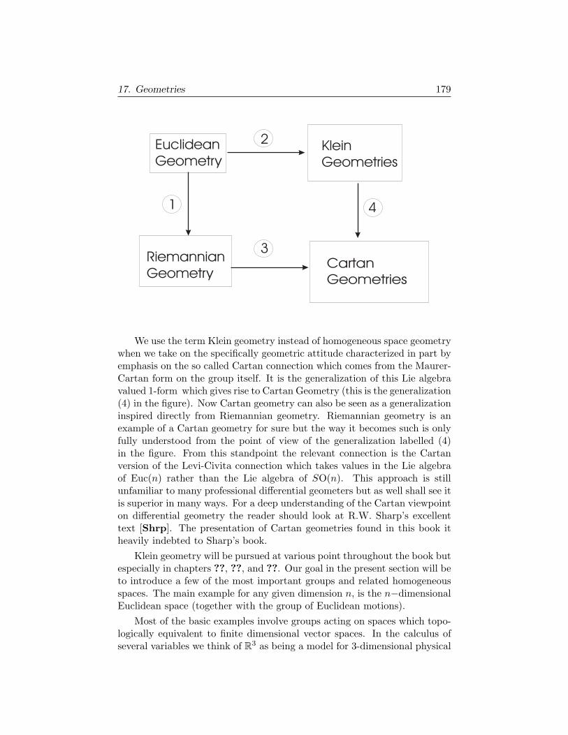
17. Geometries 179
We use the term Klein geometry instead of homogeneous space geometrywhen we take on the specifically geometric attitude characterized in part byemphasis on the so called Cartan connection which comes from the Maurer-Cartan form on the group itself. It is the generalization of this Lie algebravalued 1-form which gives rise to Cartan Geometry (this is the generalization(4) in the figure). Now Cartan geometry can also be seen as a generalizationinspired directly from Riemannian geometry. Riemannian geometry is anexample of a Cartan geometry for sure but the way it becomes such is onlyfully understood from the point of view of the generalization labelled (4)in the figure. From this standpoint the relevant connection is the Cartanversion of the Levi-Civita connection which takes values in the Lie algebraof Euc(n) rather than the Lie algebra of SO(n). This approach is stillunfamiliar to many professional differential geometers but as well shall see itis superior in many ways. For a deep understanding of the Cartan viewpointon differential geometry the reader should look at R.W. Sharp’s excellenttext [Shrp]. The presentation of Cartan geometries found in this book itheavily indebted to Sharp’s book.
Klein geometry will be pursued at various point throughout the book butespecially in chapters ??, ??, and ??. Our goal in the present section will beto introduce a few of the most important groups and related homogeneousspaces. The main example for any given dimension n, is the n−dimensionalEuclidean space (together with the group of Euclidean motions).
Most of the basic examples involve groups acting on spaces which topo-logically equivalent to finite dimensional vector spaces. In the calculus ofseveral variables we think of R3 as being a model for 3-dimensional physical
180 17. Geometries
space. Of course, everyone realizes that R3 is not quite a faithful modelof space for several reasons not the least of which is that, unlike physicalspace, R3 is a vector space and so, for instance, has a unique special element(point) called the zero element. Physical space doesn’t seem to have such aspecial point (an origin). A formal mathematical notion more appropriateto the situation which removes this idea of an origin is that of an affinespace defined below 17.1. As actors in physical space, we implicitly andsometimes explicitly impose coordinate systems onto physical space. Rect-angular coordinates are the most familiar type of coordinates that physicistsand engineers use. In the physical sciences, coordinates are really implicitin our measurement methods and in the instruments used.
We also impose coordinates onto certain objects or onto their surfaces.Particularly simple are flat surfaces like tables and so forth which intuitivelyare 2-dimensional analogues of the space in which we live. Experience withsuch objects and with 3-dimensional space itself leads to the idealizationsknown as the Euclidean plane, 3-dimensional Euclidean space. Our intuitionabout the Euclidean plane and Euclidean 3−space is extended to higher di-mensions by analogy. Like 3-dimensional space, the Euclidean plane alsohas no preferred coordinates or implied vector space structure. Euclid’s ap-proach to geometry used neither (at least no explicit use). On the otherhand, there does seem to be a special family of coordinates on the planethat makes the equations of geometry take on a simple form. These are therectangular (orthonormal) coordinates mentioned above. In rectangular co-ordinates the distance between two points is given by the usual Pythagoreanprescription involving the sum of squares. What set theoretic model shoulda mathematician exhibit as the best mathematical model of these Euclideanspaces of intuition? Well, Euclidean space may not be a vector space assuch but since we have the notion of translation in space we do have a vec-tor space “acting by translation”. Paying attention to certain features ofEuclidean space leads to the following notion:
Definition 17.1. Let A be a set and V be a vector space over a field F.We say that A is an affine space with difference space V if there is amap + : V ×A → A written (v, p) 7→ v + p such that
i) (v + w) + p = v + (w + p) for all v, w ∈ V and p ∈ A
ii) 0 + p = p for all p ∈ A.
iii) for each fixed p ∈ A the map v 7→ v + p is a bijection.
If we have an affine space with difference space V then there is a uniquemap called the difference map − : A×A → V which is defined by
q − p = the unique v ∈ V such that v + p = q.
17. Geometries 181
Thus we can form difference of two points in an affine space but we cannotadd two points in an affine space or at least if we can then that is anaccidental feature and is not part of what it means to be an affine space.We need to know that such things really exist in some sense. What shouldwe point at as an example of an affine space? In a ironic twist the set whichis most ready-to-hand for this purpose is Rn itself. We just allow Rn to playthe role of both the affine space and the difference space. We take advantageof the existence of a predefine vector addition + to provide the translationmap. Now Rn has many features that are not an essential part of its affinespace character. When we let Rn play this role as an affine space, we mustbe able to turn a sort of blind eye to features which are not essential tothe affine space structure such as the underlying vector spaces structure.Actually, it would be a bit more honest to admit that we will in fact usefeatures of Rn which are accidental to the affine space structure. After all,the first thing we did was to use the vector space addition from Rn to providethe translation map. This is fine- we only need to keep track of what aspectsof our constructions and which of our calculations retain significant for theproperly affine aspects of Rn. The introduction of group theory into thepicture helps a great deal in sorting things out. More generally any vectorspace can be turned into an affine space simply by letting the translationoperator + required by the definition of an affine space to be the additionthat is part of the vector space structure of V . This is just the same as whatwe did with Rn and again V itself is its own difference space and the setV is playing two roles. Similar statements apply it the field is C. In fact,algebraic geometers refer to Cn as complex affine space.
Let F be one of the fields R or C. Most of the time R is the field intendedwhen no specification is made. It is a fairly common practice to introducemultiple notations for the same set. For example, when we think of thevector space Fn as an affine space we sometimes denote it by An(F) or justAn if the underlying field is understood.
Definition 17.2. If Ai is an affine space with difference space Vi for i = 1, 2then we say that a map F : A1 → A2 is an affine transformation if it hasthe form x 7→ F (x0)+L(x−x0) for some linear transformation L : V1 → V2.
It is easy to see that for a fixed point p in an affine space A we immedi-ately obtain a bijection V → A which is given by v 7→ p + v. The inverse ofthis bijection is a map cp : A → V which we put to use presently. An affinespace always has a globally defined coordinate system. To see this pick abasis for V . This gives a bijection V → Rn. Now choose a point p ∈ Aand compose with the canonical bijection cp : A → V just mentioned. Thisa coordinates system. Any two such coordinate systems are related by an
182 17. Geometries
bijective affine transformation (an affine automorphism). These special co-ordinate systems can be seen as an alternate way of characterizing the affinestructure on the set A. In fact, singling out a family of specially relatedcoordinate systems is an often used method saying what we mean when wesay that a set has a structure of a given type and this idea will be encounterrepeatedly.
If V is a finite dimensional vector space then it has a distinguished topol-ogy3 which is transferred to the affine space using the canonical bijections.Thus we may consider open sets in A and also continuous functions on opensets. Now it is usually convenient to consider the “coordinate representa-tive” of a function rather than the function itself. By this we mean thatif x : A → Rn is a affine coordinate map as above, then we may replace afunction f : U ⊂ A → R (or C) by the composition f x. The latter is oftendenoted by f(x1, ..., xn). Now this coordinate representative may, or maynot, turn out to be a differentiable function but if it is then all other coordi-nate representatives of f obtained by using other affine coordinate systemswill also be differentiable. For this reason, we may say that f itself is (oris not) differentiable. We say that the family of affine coordinate systemsprovide the affine space with a differentiable structure and this means thatevery (finite dimensional) affine space is also an example of differentiablemanifold (defined later). In fact, one may take the stance that an affinespace is the local model for all differentiable manifolds.
Another structure that will seem a bit trivial in the case of an affinespace but that generalizes in a nontrivial way is the idea of a tangent space.We know what it means for a vector to be tangent to a surface at a pointon the surface but the abstract idea of a tangent space is also exemplifiedin the setting of affine spaces. If we have a curve γ : (a, b) ⊂ R → A thenthe affine space structure allows us to make sense of the difference quotient
γ(t0) := limh→0
γ(t0 + h)− γ(t0)h
, t0 ∈ (a, b)
which defines an element of the difference space V (assuming the limit ex-ists). Intuitively we think of this as the velocity of the curve based at γ(t0).We may want to explicitly indicate the base point. If p ∈ A, then the tan-gent space at p is p × V and is often denoted by TpA. The set of alltangent spaces for points in an open set U ⊂ A is called the tangent bun-dle over U and is another concept that will generalize in a very interestingway. Thus we have not yet arrived at the usual (metric) Euclidean space orEuclidean geometry where distances and angle are among the prominent no-tions. On the other hand, an affine space supports a geometry called affinegeometry. The reader who has encountered axiomatic affine geometry will
3If V is infinite dimensional we shall usually assume that V is a topological vector space.
17.1. Group Actions, Symmetry and Invariance 183
remember that one is mainly concerned about lines and the their mutualpoints of incidence. In the current analytic approach a line is the set of im-age points of an affine map a : R→A. We will not take up affine geometryproper. Rather we shall be mainly concerned with geometries that resultfrom imposing more structure on the affine space. For example, an affinespace is promoted to a metric Euclidean space once we introduce length andangle. Once we introduce length and angle into Rn it becomes the standardmodel of n-dimensional Euclidean space and might choose to employ thenotation En instead of Rn. The way in which length and angle is introducedinto Rn (or an abstract finite dimensional vector space V ) is via an innerproduct and this is most likely familiar ground for the reader. Nevertheless,we will take closer look at what is involved so that we might place Euclideangeometry into a more general context. In order to elucidate both affine ge-ometry and Euclidean geometry and to explain the sense in which the wordgeometry is being used, it is necessary to introduce the notion of “groupaction”.
17.1. Group Actions, Symmetry and Invariance
One way to bring out the difference between Rn, An and En, which are allthe same considered as sets, is by noticing that each has its own natural setof coordinates and coordinate transformations. The natural family of coor-dinate systems for An are the affine coordinates and are related amongstthemselves by affine transformations under which lines go to lines (planes toplanes etc.). Declaring that the standard coordinates obtained by recallingthat An = Rn determines all other affine coordinate systems. For En thenatural coordinates are the orthonormal rectangular coordinates which arerelated to each other by affine transformations whose linear parts are orthog-onal transformations of the difference space. These are exactly the lengthpreserving transformations or isometries. We will make this more explicitbelow but first let us make some comments about the role of symmetry ingeometry.
We assume that the reader is familiar with the notion of a group. Mostof the groups that play a role in differential geometry are matrix groupsand are the prime examples of so called ‘Lie groups’ which we study indetail later in the book. For now we shall just introduce the notion of atopological group. All Lie groups are topological groups. Unless otherwiseindicated finite groups G will be given the discreet topology where everysingleton g ⊂ G is both open and closed.
Definition 17.3. Let G be a group. We say that G is a topological group ifG is also a topological space and if the maps µ : G×G → G and inv : G → G,given by (g1, g2) → g1g2 and g1 7→ g−1 respectively, are continuous maps.
184 17. Geometries
If G is a countable or finite set we usually endow G with the discretetopology so that in particular, every point would be an open set. In thiscase we call G a discrete group.
Even more important for our present discussion is the notion of a groupaction. Recall that if M is a topological space then so is G ×M with theproduct topology.
Definition 17.4. Let G and M be as above. A left (resp. right) groupaction is a map α : G ×M → M (resp. α : M × G → M) such that forevery g ∈ G the partial map αg(.) := α(g, .) (resp. α,g(.) := α(., g)) iscontinuous and such that the following hold:
1) α(g2, α(g1, x)) = α(g2g1, x) (resp. α(α(x, g1), g2) = α(x, g1g2)) for allg1, g2 ∈ G and all x ∈ M .
2) α(e, x) = x (resp. α(x, e) = x) for all x ∈ M.
It is traditional to write g · x or just gx in place of the more pedanticnotation α(g, x). Using this notation we have g2 · (g1 · x) = (g2g1) · x ande · x = x.
We shall restrict our exposition for left actions only since the correspond-ing notions for a right action are easy to deduce. Furthermore, if we havea right action x → αR(x, g) then we can construct an essentially equivalentleft action by αL : x → αL(g, x) := αR(x, g−1).
If we have an action α : G × M → M then for a fixed x, the setG · x := g · x : g ∈ G is called the orbit of x. The set of orbits is denotedby M/G or sometimes G|M if we wish to emphasize that the action is a leftaction. It is easy to see that two orbits G · x and G · y are either disjoint oridentical and so define an equivalence relation. The natural projection ontoset of orbits p : M → M/G is given by
x 7→ G · x.
If we give M/G the quotient topology then of course p is continuous.
Definition 17.5. If G acts on M the we call M a G-space.
Exercise 17.6. Convince yourself that an affine space A with differencespace V is a V−space where we consider V as an abelian group underaddition.
Definition 17.7. Let G act on M1 and M2. A map f : M1 → M2 is calleda G−map if
f(g · x) = g · f(x)
17.1. Group Actions, Symmetry and Invariance 185
for all x ∈ M and all g ∈ G. If f is a bijection then we say that f is aG-automorphism and that M1 and M2 are isomorphic as G-spaces. Moregenerally, if G1 acts on M1 and G2 acts on M2 then a weak group actionmorphism from M1 to M2 is a pair of maps (f, φ) such that
(i) f : M1 → M2 ,(ii) φ : G1 → G2 is a group homomorphism and(iii) f(g ·x) = φ(g) · f(x) for all x ∈ M and all g ∈ G. If f is a bijection andφ is an isomorphism then the group actions on M1 and M2 are equivalent.
We have refrained from referring to the equivalence in (iii) as a “weak”equivalence since if M1 and M2 are G1 and G2 spaces respectively which areequivalent in the sense of (iii) then G1
∼= G2 by definition. Thus if we thenidentify G1 and G2 and call the resulting abstract group G then we recovera G−space equivalence between M1 and M2.
One main class of examples are those where M is a vector space (say V )and each αg is a linear isomorphism. In this case, the notion of a left groupaction is identical to what is called a group representation and for eachg ∈ G, the map g 7→ αg is a group homomorphism4 with image in the spaceGL(V ) of linear isomorphism of G to itself. The most common groups thatoccur in geometry are matrix groups, or rather, groups of automorphisms ofa fixed vector space. Thus we are first to consider subgroups of GL(V ). Atypical way to single out subgroups of GL(V ) is provided by the introductionof extra structure onto V such as an orientation and/or a special bilinearform such as an real inner product, Hermitian inner product, or a symplecticfrom to name just a few. We shall introduce the needed structures and thecorresponding groups as needed. As a start we ask the reader to recallthat an automorphism of a finite dimensional vector space V is orientationpreserving if its matrix representation with respect to some basis has positivedeterminant. (A more geometrically pleasing definition of orientation andof determinant etc. will be introduced later). The set of all orientationpreserving automorphisms of V is denoted a subgroup of GL(V ) and isdenoted Gl+(V ) and referred to as the proper general linear group. Weare also interested in the group of automorphisms that have determinantequal to 1 which gives us a “special linear group”. (These will be seento be volume preserving maps). Of course, once we pick a basis we getan identification of any such linear automorphism group with a group ofmatrices. For example, we identify GL(Rn) with the group GL(n,R) ofnonsingular n× n matrices. Also, Gl+(Rn) ∼= Gl+(n,R) = A ∈ GL(n,R) :detA = 1. A fairly clear pattern of notation is emerging and we shall notbe so explicit about the meaning of the notation in the sequel.
4A right group action does not give rise to a homomorphism but an “anti-homomorphism”.
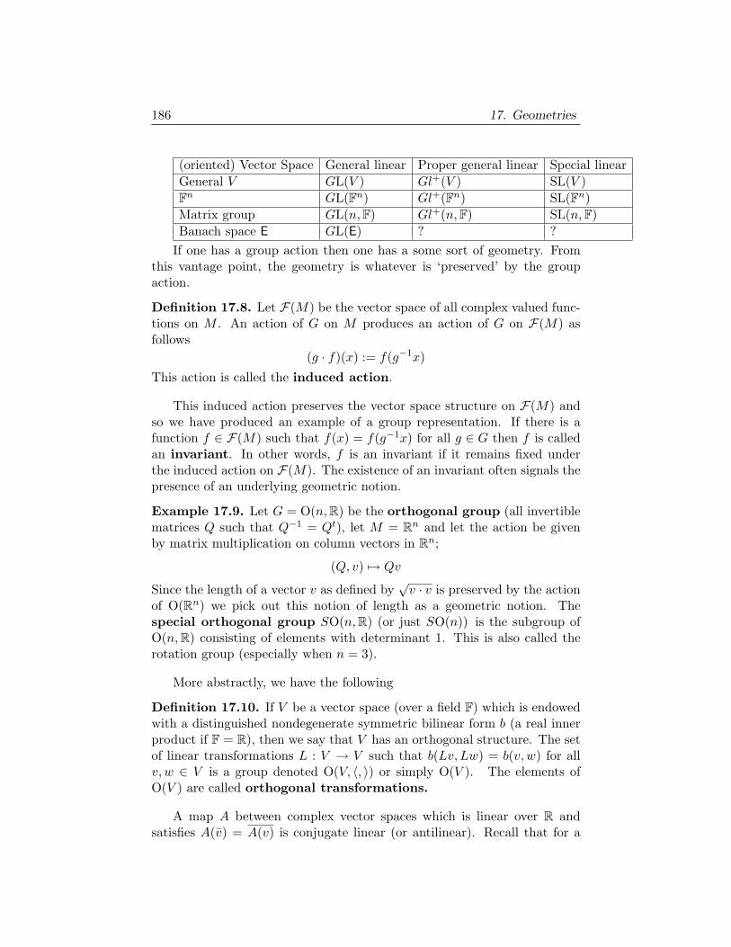
186 17. Geometries
(oriented) Vector Space General linear Proper general linear Special linearGeneral V GL(V ) Gl+(V ) SL(V )Fn GL(Fn) Gl+(Fn) SL(Fn)Matrix group GL(n,F) Gl+(n,F) SL(n,F)Banach space E GL(E) ? ?
If one has a group action then one has a some sort of geometry. Fromthis vantage point, the geometry is whatever is ‘preserved’ by the groupaction.
Definition 17.8. Let F(M) be the vector space of all complex valued func-tions on M . An action of G on M produces an action of G on F(M) asfollows
(g · f)(x) := f(g−1x)
This action is called the induced action.
This induced action preserves the vector space structure on F(M) andso we have produced an example of a group representation. If there is afunction f ∈ F(M) such that f(x) = f(g−1x) for all g ∈ G then f is calledan invariant. In other words, f is an invariant if it remains fixed underthe induced action on F(M). The existence of an invariant often signals thepresence of an underlying geometric notion.
Example 17.9. Let G = O(n,R) be the orthogonal group (all invertiblematrices Q such that Q−1 = Qt), let M = Rn and let the action be givenby matrix multiplication on column vectors in Rn;
(Q, v) 7→ Qv
Since the length of a vector v as defined by√
v · v is preserved by the actionof O(Rn) we pick out this notion of length as a geometric notion. Thespecial orthogonal group SO(n,R) (or just SO(n)) is the subgroup ofO(n,R) consisting of elements with determinant 1. This is also called therotation group (especially when n = 3).
More abstractly, we have the following
Definition 17.10. If V be a vector space (over a field F) which is endowedwith a distinguished nondegenerate symmetric bilinear form b (a real innerproduct if F = R), then we say that V has an orthogonal structure. The setof linear transformations L : V → V such that b(Lv, Lw) = b(v, w) for allv, w ∈ V is a group denoted O(V, 〈, 〉) or simply O(V ). The elements ofO(V ) are called orthogonal transformations.
A map A between complex vector spaces which is linear over R andsatisfies A(v) = A(v) is conjugate linear (or antilinear). Recall that for a
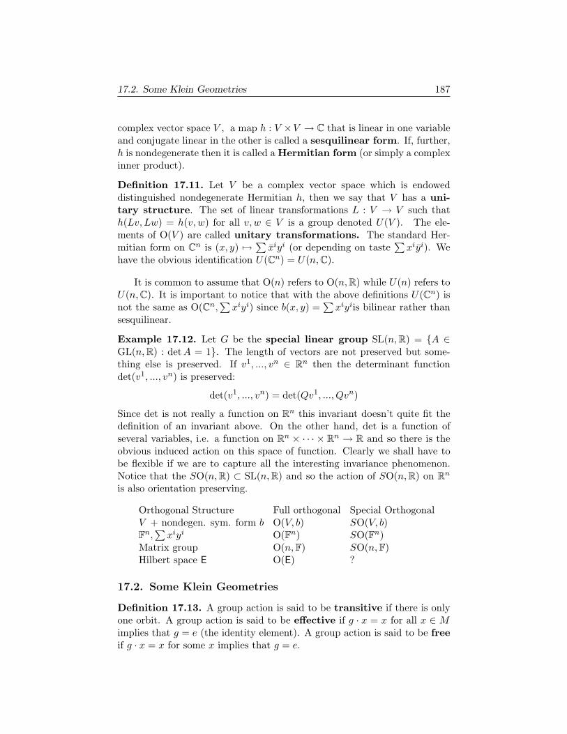
17.2. Some Klein Geometries 187
complex vector space V , a map h : V ×V → C that is linear in one variableand conjugate linear in the other is called a sesquilinear form. If, further,h is nondegenerate then it is called a Hermitian form (or simply a complexinner product).
Definition 17.11. Let V be a complex vector space which is endoweddistinguished nondegenerate Hermitian h, then we say that V has a uni-tary structure. The set of linear transformations L : V → V such thath(Lv,Lw) = h(v, w) for all v, w ∈ V is a group denoted U(V ). The ele-ments of O(V ) are called unitary transformations. The standard Her-mitian form on Cn is (x, y) 7→ ∑
xiyi (or depending on taste∑
xiyi). Wehave the obvious identification U(Cn) = U(n,C).
It is common to assume that O(n) refers to O(n,R) while U(n) refers toU(n,C). It is important to notice that with the above definitions U(Cn) isnot the same as O(Cn,
∑xiyi) since b(x, y) =
∑xiyiis bilinear rather than
sesquilinear.
Example 17.12. Let G be the special linear group SL(n,R) = A ∈GL(n,R) : detA = 1. The length of vectors are not preserved but some-thing else is preserved. If v1, ..., vn ∈ Rn then the determinant functiondet(v1, ..., vn) is preserved:
det(v1, ..., vn) = det(Qv1, ..., Qvn)
Since det is not really a function on Rn this invariant doesn’t quite fit thedefinition of an invariant above. On the other hand, det is a function ofseveral variables, i.e. a function on Rn × · · · × Rn → R and so there is theobvious induced action on this space of function. Clearly we shall have tobe flexible if we are to capture all the interesting invariance phenomenon.Notice that the SO(n,R) ⊂ SL(n,R) and so the action of SO(n,R) on Rn
is also orientation preserving.
Orthogonal Structure Full orthogonal Special OrthogonalV + nondegen. sym. form b O(V, b) SO(V, b)Fn,
∑xiyi O(Fn) SO(Fn)
Matrix group O(n,F) SO(n,F)Hilbert space E O(E) ?
17.2. Some Klein Geometries
Definition 17.13. A group action is said to be transitive if there is onlyone orbit. A group action is said to be effective if g · x = x for all x ∈ Mimplies that g = e (the identity element). A group action is said to be freeif g · x = x for some x implies that g = e.
188 17. Geometries
Klein’s view is that a geometry is just a transitive G-space. Whateverproperties of figures (or more general objects) that remain unchanged underthe action of G are deemed to be geometric properties by definition.
Example 17.14. We give an example of an SL(n,R)-space as follows: LetM be the upper half complex plane z ∈ C : Im z > 0. Then the action ofSL(n,R) on M is given by
(A, z) 7→ az + b
cz + d
where A =(
a bc d
).
Exercise 17.15. Let A ∈ SL(n,R) as above and w = A · z = az+bcz+d . Show
that if Im z > 0 then Imw > 0 so that the action of the last example is welldefined.
17.2.1. Affine Space. Now let us consider the notion of an affine spaceagain. Careful attention to the definitions reveals that an affine space is aset on which a vector space acts (a vector space is also an abelian groupunder the vector addition +). We can capture more of what an affine spaceAn is geometrically by enlarging this action to include the full group ofnonsingular affine maps of An onto itself. This group is denoted Aff(An)and is the set of transformations of An of the form A : x 7→ Lx0 +L(x−x0)for some L ∈ GL(n,R) and some x0 ∈ An. More abstractly, if A is an affinespace with difference space V then we have the group of all transformationsof the form A : x 7→ Lx0 + L(x−x0) for some x0 ∈ A and L ∈ GL(V ). Thisis the affine group associated with A and is denoted by Aff(A). Using ourprevious terminology, A is an Aff(A)−space. An (= Rn) is our standardmodel of an n-dimensional affine space. It is an Aff(An)-space.
Exercise 17.16. Show that if A an is a n-dimensional affine space withdifference space V then Aff(A)∼= Aff(An) and the Aff(A)-space A is equiv-alent to the Aff(An)−space An.
Because of the result of this last exercise it is sufficient mathematicallyto restrict the study of affine space to the concrete case of An the reasonthat we refer to An as the standard affine space. We can make things evennicer by introducing a little trick which allows us to present Aff(An) as amatrix group. Let An be identified with the set of column vectors in Rn+1
of the form [1x
]where x ∈ Rn
17.2. Some Klein Geometries 189
The set of all matrices of the form[1 0x0 L
]where Q ∈ GL(n,R) and x0 ∈ Rn
is a group. Now [1 0x0 L
] [1x
]=
[1
Lx + x0
]
Remember that affine transformations of An (= Rn as a set) are of the formx 7→ Lx+x0. In summary, when we identify An with the vectors of the form[
1x
]then the group Aff(An) is the set of (n + 1)× (n + 1) matrices of the
form indicated and the action of Aff(An) is given by matrix multiplication.It is often more appropriate to consider the proper affine group
Aff+(A, V ) obtained by adding in the condition that its elements havethe form A : x 7→ Lx0 + L(x− x0) with detL > 0.
We have now arrive at another meaning of affine space. Namely, the sys-tem (A, V, Aff+(A), ·, +). What is new is that we are taking the action “·”of Aff+(A) on as part of the structure so that now A is an Aff+(A)−space.
Exercise 17.17. Show that the action of V on A is transitive and free.Show that the action of Aff+(A) on A is transitive and effective but notfree.
Affine geometry is the study of properties attached to figures in an affinespace that remain, in some appropriate sense, unchanged under the action ofthe affine group (or the proper affine group Aff+). For example, coincidenceproperties of lines and points are preserved by Aff .
17.2.2. Special Affine Geometry. We can introduce a bit more rigidityinto affine space by changing the linear part of the group to SL(n).
Definition 17.18. The group SAff(A) of affine transformations of anaffine space A that are of the form
A : x 7→ Lx0 + L(x− x0)
with detL = 1 will be called the special affine group.
We will restrict ourselves to the standard model of An. With this newgroup the homogeneous space structure is now different and the geometryhas changed. For one thing volume now makes sense. The are many similar-ities between special affine geometry and Euclidean geometry. As we shallsee in chapter ??, in dimension 3, there exist special affine versions of arclength and surface area and mean curvature.
The volume of a parallelepiped is preserved under this action.
190 17. Geometries
17.2.3. Euclidean space. Suppose now that we have an affine space (A, V,+)together with an inner product on the vector space V . Consider the groupof affine transformations the form A : x 7→ Lx0 + L(x − x0) where nowL ∈ O(V ). This is called the Euclidean motion group of A. Then A be-comes, in this context, a Euclidean space and we might choose a differentsymbol, say E for the space to encode this fact. For example, when Rn isreplaced by En and the Euclidean motion group is denoted Euc(En).
Remark: Now every tangent space TpA = p × V inherits the innerproduct from V in the obvious and trivial way. This is our first example ofa metric tensor. Having a metric tensor on the more general spaces that westudy later on will all us to make sense of lengths of curves, angles betweenvelocity curves, volumes of subsets and much more.
In the concrete case of En (secretly Rnagain) we may represent theEuclidean motion group Euc(En) as a matrix group, denoted Euc(n), byusing the trick we used before. If we want to represent the transformationx → Qx+b where x, b ∈ Rn and Q ∈ O(n,R), we can achieve this by lettingcolumn vectors [
1x
]∈ Rn+1
represent elements x. Then we take the group of matrices of the form[1 0b Q
]
to play the role of Euc(n). This works because[
1 0b Q
] [1x
]=
[1
b + Qx
].
The set of all coordinate systems related to the standard coordinates byan element of Euc(n) will be called Euclidean coordinates (or sometimesorthonormal coordinates). It is these coordinate which we should use tocalculate distance.
Basic fact 1: The (square of the) distance between two points inEn can be calculated in any of the equivalent coordinate systems by theusual formula. This means that if P, Q ∈ En and we have some Eu-clidean coordinates for these two points: x(P ) = (x1(P ), ..., xn(P )), x(Q) =(x1(Q), ..., xn(Q)) then vector difference in these coordinates is ∆x = x(P )−x(Q) = (∆x1, ...,∆xn). If y = (y1, ...., yn) are any other coordinates relatedto x by y = Tx for some T ∈ Euc(n) then we have
∑(∆yi)2 =
∑(∆xi)2
where ∆y = y(P ) − y(Q) etc. The distance between two points in a Eu-clidean space is a simple example of a geometric invariant.
Let us now pause to consider again the abstract setting of G−spaces. Isthere geometry here? We will not attempt to give an ultimate definition of
17.2. Some Klein Geometries 191
geometry associated to a G−space since we don’t want to restrict the direc-tion of future generalizations. Instead we offer the following two (somewhattentative) definitions:
Definition 17.19. Let M be a G−space. A figure in M is a subset ofM . Two figures S1, S2 in M are said to be geometrically equivalent orcongruent if there exists an element g ∈ G such that g · S1 = S2.
Definition 17.20. Let M be a G−space and let S be some family of figuresin M such that g · S ∈ S whenever .S ∈ S . A function I : S → C is calleda (complex valued) geometric invariant if I(g · S) = I(S) for all S ∈ S.
Example 17.21. Consider the action of O(n) on En. Let S be the family ofall subsets of En which are the images of C1 of the form c : [a, b] → En suchthat c′ is never zero (regular curves). Let S ∈ S be such a curve. Takingsome regular C1map c such that S is the image of c we define the length
L(S) =∫ b
a
∥∥c′(t)∥∥ dt
It is common knowledge that L(S) is independent of the parameterizing mapc and so L is a geometric invariant (this is a prototypical example)
Notice that two curves may have the same length without being con-gruent. The invariant of length by itself does not form a complete set ofinvariants for the family of regular curves S. The definition we have inmind here is the following:
Definition 17.22. Let M be a G−space and let S be some family of figuresin M . Let I = Iαα∈A be a set of geometric invariants for S. We say thatI is a complete set of invariants if for every S1, S2 ∈ S we have that S1 iscongruent to S2 if and only if Iα(S1) = Iα(S2) for all α ∈ A.
Example 17.23. Model Euclidean space by R3 and consider the familyC of all regular curves c : [0, L] → R3 such that dc
dt and d2cdt2
never vanish.Each such curve has a parameterization by arc length which we may takeadvantage of for the purpose of defining a complete set of invariant for suchcurves. Now let c : [0, L] → R3 a regular curve parameterized by arc length.Let
T(s) :=dcdt (s)∣∣dcdt (s)
∣∣define the unit tangent vector field along c. The curvature is an invariantdefined on c that we may think of as a function of the arc length parameter.It is defined by κ(s) :=
∣∣dcdt (s)
∣∣. We define two more fields along c. Firstthe normal field is defined by N(s) = dc
dt (s). Next, define the unit binormal
192 17. Geometries
vector field B by requiring that T,N,B is a positively oriented triple oforthonormal unit vectors. By positively oriented we mean that
det[T,N,B] = 1.
We now show that dNds is parallel to B. For this it suffices to show that dN
dsis normal to both T and N. First, we have N(s) ·T(s) = 0. If this equationis differentiated we obtain 2dN
ds ·T(s) = 0. On the other hand we also have1 = N(s) ·N(s) which differentiates to give 2dN
ds ·N(s) = 0. From this wesee that there must be a function τ = τ(s) such that dN
ds := τB. This is afunction of arc length but should really be thought of as a function on thecurve. This invariant is called the torsion. Now we have a matrix definedso that
d
ds[T,N,B] = [T,N,B]
0 κ 0−κ 0 τ0 τ 0
or in other wordsdTds = κNdNds = −κT τBdBds = τN
Since F = [T,N,B] is by definition an orthogonal matrix we have F (s)F t(s) =I. It is also clear that there is some matrix function A(s) such that F ′ =F (s)A(s). Also, Differentiating we have dF
ds (s)F t(s) + F (s)dFds
t(s) = 0 and
so
FAF t + FAtF t = 0
A + At = 0
since F is invertible. Thus A(s) is antisymmetric. But we already haveestablished that dT
ds = κN and dBds = τN and so the result follows. It can
be shown that the functions κ and τ completely determine a sufficientlyregular curve up to reparameterization and rigid motions of space. Thethree vectors form a vector field along the curve c. At each point p = c(s)along the curve c the provide and oriented orthonormal basis ( or frame)for vectors based at p. This basis is called the Frenet frame for the curve.Also, κ(s) and τ(s) are called the (unsigned) curvature and torsion of thecurve at c(s). While, κ is never negative by definition we may well havethat τ(s) is negative. The curvature is, roughly speaking, the reciprocal ofthe radius of the circle which is tangent to c at c(s) and best approximatesthe curve at that point. On the other hand, τ measures the twisting of theplane spanned by T and N as we move along the curve. If γ : I → R3 isan arbitrary speed curve then we define κγ(t) := κ h−1 where h : I ′ → Igives a unit speed reparameterization c = γh : I ′ → Rn. Define the torsion
17.2. Some Klein Geometries 193
function τγ for γ by τ h−1. Similarly we have
Tγ(t) := T h−1(t)
Nγ(t) := Nh−1(t)
Bγ(t) := Bh−1(t)
Exercise 17.24. If c : I → R3 is a unit speed reparameterization of γ :I → R3 according to γ(t) = c h then show that
(1) Tγ(t) = γ′/ ‖γ′‖(2) Nγ(t) = Bγ(t)×Tγ(t)
(3) Bγ(t) = γ′×γ′′‖γ′×γ′′‖
(4) κγ = ‖γ′×γ′′‖‖γ′′‖3
(5) τγ = (γ′×γ′′)·γ′′′‖γ′×γ′′‖2
Exercise 17.25. Show that γ′′ = dvdt Tγ + v2κγNγ where v = ‖γ′‖.
Example 17.26. For a curve confined to a plane we haven’t got the op-portunity to define B or τ . However, we can obtain a more refined notionof curvature. We now consider the special case of curves in R2. Here it ispossible to define a signed curvature which will be positive when the curveis turning counterclockwise. Let J : R2 → R2 be given by J(a, b) := (−b, a).The signed curvature κ±γ of γ is given by
κ±γ (t) :=γ′′(t) · Jγ′(t)‖γ′(t)‖3 .
If γ is a parameterized curve in R2 then κγ ≡ 0 then γ (parameterizes) astraight line. If κγ ≡ k0 > 0 (a constant) then γ parameterizes a portion ofa circle of radius 1/k0. The unit tangent is T = γ′
‖γ′‖ . We shall redefine thenormal N to a curve to be such that T,N is consistent with the orientationgiven by the standard basis of R2.
Exercise 17.27. If c : I → R2 is a unit speed curve then
(1) dTds (s) = κc(s)N(s)
(2) c′′(s) = κc(s) (JT(s))
Example 17.28. Consider the action of Aff+(2) on the affine plane A2.Let S be the family of all subsets of A2 which are zero sets of quadraticpolynomials of the form
ax2 + bxy + cy2 + dx + ey + f.
with the nondegeneracy condition 4ac − b2 6= 0. If S is simultaneously thezero set of nondegenerate quadratics p1(x, y) and p2(x, y) then p1(x, y) =
194 17. Geometries
p2(x, y). Furthermore, if g · S1 = S2 where S1 is the zero set of p1 then S2
is the zero set of the nondegenerate quadratic polynomial p2 := p1 g−1.A little thought shows that we may as well replace S by the set of set ofnondegenerate quadratic polynomials and consider the induced action onthis set: (g, p) 7→ p g−1. We may now obtain an invariant: Let S = p−1(0)and let I(S) =: I(p) =: sgn(4ac− b2) where p(x, y) = ax2 + bxy + cy2 +dx+ey + f . In this case, S is divided into exactly two equivalence classes
Notice that in example 17.21 above the set of figures considered wasobtained as the set of images for some convenient family of maps into theset M . This raises the possibility of a slight change of viewpoint: maybewe should be studying the maps themselves. Given a G-set M , we couldconsider a family of maps C from some fixed topological space T (or familyof topological spaces like intervals in R say) into M which is invariant in thesense that if c ∈ C then the map g ·c defined by g ·c : t 7→ g ·c(t) is also in C.Then two elements c1 and c2 would be “congruent” if and only if g · c1 = c2
for some g ∈ G. Now suppose that we find a function I : C →C which is aninvariant in the sense that I(g · c) = I(c) for all c ∈ C and all g ∈ G. Wedo not necessarily obtain an invariant for the set of images of maps from C.For example, if we consider the family of regular curves c : [0, 1] → E2 andlet G = O(2) with the action introduced earlier, then the energy functionaldefined by
E(c) :=∫ 1
0
12
∥∥c′(t)∥∥2
dt
is an invariant for the induced action on this set of curves but even if c1 andc2 have the same image it does not follow that E(c1) = E(c2). Thus E isa geometric invariant of the curve but not of the set which is its image. Inthe elementary geometric theory of curves in Euclidean spaces one certainlywants to understand curves as sets. One starts out by studying the mapsc : I → En first. In order to get to the geometry of the subsets which areimages of regular curves one must consider how quantities defined depend onthe choice of parameterization. Alternatively, a standard parameterization(parameterization by arc length) is always possible and this allows one toprovide geometric invariants of the image sets (see Appendix ??) .
Similarly, example 17.22 above invites us to think about maps from Minto some topological space T (like R for example). We should pick a familyof maps F such that if f ∈ F then g·f is also in F where g·f : x 7→ f(g−1 ·x).Thus we end up with G acting on the set F . This is an induced action. Wehave chosen to use g−1 in the definition so that we obtain a left action onF rather than a right action. In any case, we could then consider f1 andf2 to be congruent if g · f1 = f2 for some g ∈ G.
17.2. Some Klein Geometries 195
There is much more to the study of figure in Euclidean space than wehave indicated here. We prefer to postpone introduction of these conceptsuntil after we have a good background in manifold theory and then intro-duce the more general topic of Riemannian geometry. Under graduate leveldifferential geometry courses usually consist mostly of the study of curvesand surfaces in 3−dimensional Euclidean space and the reader who has beenexposed to this will already have an idea of what I am talking about. Aquick review of curves and surfaces is provided in appendix ??. The studyof Riemannian manifolds and submanifolds that we take up in chapters ??and ??.
We shall continue to look at simple homogeneous spaces for inspirationbut now that we are adding in the notion of time we might try thinking ina more dynamic way. Also, since the situation has become decidedly morephysical it would pay to start considering the possibility that the questionof what counts as geometric might be replaced by the question of whatcounts as physical. We must eventually also ask what other group theoreticprincipals (if any) are need to understand the idea of invariants of motionsuch as conservation laws.
17.2.4. Galilean Spacetime. Spacetime is the set of all events in a (fornow 4 dimensional) space. At first it might seem that time should be in-cluded by simply taking the Cartesian product of space E3 with a copy ofR that models time: Spacetime=Space×R. Of course, this leads directly toR4, or more appropriately to E3×R. Topologically this is right but the waywe have written it implies an inappropriate and unphysical decomposition oftime and space. If we only look at (affine) self transformations of E3×R thatpreserve the decomposition then we are looking at what is sometimes calledAristotelean spacetime (inappropriately insulting Aristotel). The problemis that we would not be taking into account the relativity of motion. If twospaceships pass each other moving a constant relative velocity then who isto say who is moving and who is still (or if both are moving). The decom-position A4 = R4 = E3 × R suggests that a body is at rest if and only ifit has a career (worldline) of the form p × R; always stuck at p in otherwords. But relativity of constant motion implies that no such assertion canbe truly objective relying as it does on the assumption that one coordinatesystem is absolutely “at rest”. Coordinate transformations between two setsof coordinates on 4−dimensional spacetime which are moving relative to oneanother at constant nonzero velocity should mix time and space in some way.There are many ways of doing this and we must make a choice. The firstconcept of spacetime that we can take seriously is Galilean spacetime. Herewe lose absolute motion (thankfully) but retain an absolute notion of time.In Galilean spacetime, it is entirely appropriate to ask whether two events
196 17. Geometries
are simultaneous or not. Now the idea that simultaneity is a well define isvery intuitive but we shall shortly introduce Minkowski spacetime as morephysically realistic and then discover that simultaneity will become a merelyrelative concept! The appropriate group of coordinate changes for Galileanspacetime is the Galilean group and denoted by Gal. This is the groupof transformations of R4 (thought of as an affine space) generated by thefollow three types of transformations:
(1) Spatial rotations: These are of the form
txyz
7→
1 0 0 000 R0
txyz
where R ∈ O(3),(2) Translations of the origin
txyz
7→
txyz
+
t0x0
y0
z0
for some (t0, x0, y0, z0) ∈ R4.(3) Uniform motions. These are transformations of the form
txyz
7→
tx + v1ty + v2tz + v3t
for some (velocity) v = (v1, v2, v3). The picture here is that thereare two observers each making measurements with respect to theirown rectangular spatial coordinate systems which are moving rela-tive to each other with a constant velocity v. Each observer is ableto access some universally available clock or synchronized systemof clock which will give time measurements that are unambiguousexcept for choice of the “zero time” (and choice of units which wewill assume fixed).
The set of all coordinates related to the standard coordinates of R4 byan element of Gal will be referred to as Galilean inertial coordinates. Whenthe set R4 is provided with the action by the Galilean group we refer to ita Galilean spacetime. We will not give a special notation for the space. Asa matter of notation it is common to denoted (t, x, y, z) by (x0, x1, x2, x3).The spatial part of an inertial coordinate system is sometimes denoted byr := (x, y, z) = (x1, x2, x3).
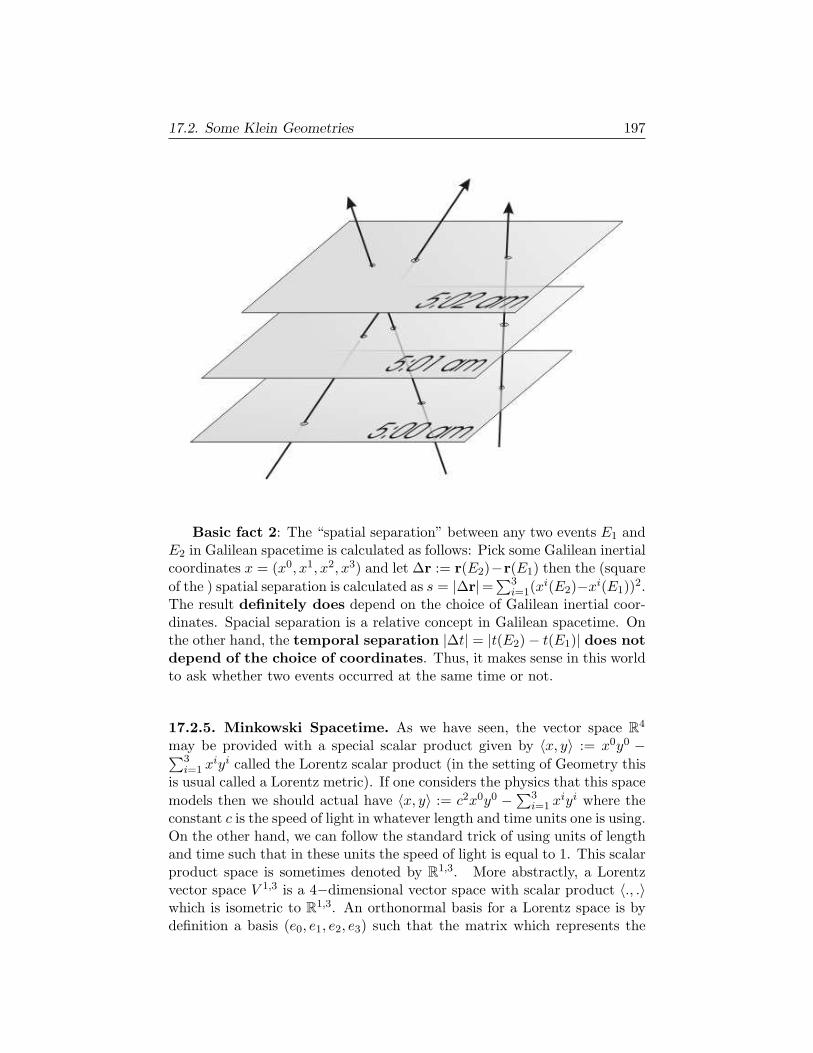
17.2. Some Klein Geometries 197
Basic fact 2: The “spatial separation” between any two events E1 andE2 in Galilean spacetime is calculated as follows: Pick some Galilean inertialcoordinates x = (x0, x1, x2, x3) and let ∆r := r(E2)−r(E1) then the (squareof the ) spatial separation is calculated as s = |∆r|=∑3
i=1(xi(E2)−xi(E1))2.
The result definitely does depend on the choice of Galilean inertial coor-dinates. Spacial separation is a relative concept in Galilean spacetime. Onthe other hand, the temporal separation |∆t| = |t(E2)− t(E1)| does notdepend of the choice of coordinates. Thus, it makes sense in this worldto ask whether two events occurred at the same time or not.
17.2.5. Minkowski Spacetime. As we have seen, the vector space R4
may be provided with a special scalar product given by 〈x, y〉 := x0y0 −∑3i=1 xiyi called the Lorentz scalar product (in the setting of Geometry this
is usual called a Lorentz metric). If one considers the physics that this spacemodels then we should actual have 〈x, y〉 := c2x0y0 −∑3
i=1 xiyi where theconstant c is the speed of light in whatever length and time units one is using.On the other hand, we can follow the standard trick of using units of lengthand time such that in these units the speed of light is equal to 1. This scalarproduct space is sometimes denoted by R1,3. More abstractly, a Lorentzvector space V 1,3 is a 4−dimensional vector space with scalar product 〈., .〉which is isometric to R1,3. An orthonormal basis for a Lorentz space is bydefinition a basis (e0, e1, e2, e3) such that the matrix which represents the
198 17. Geometries
scalar product with respect to basis is
η =
−1 0 0 00 1 0 00 0 1 00 0 0 1
Once we pick such a basis for a Lorentz space we get an isomorphism withR1,3. Physically and geometrically, the standard basis of R1,3 is just oneamong many orthonormal bases so if one is being pedantic, the abstractspace V 1,3 would be more appropriate. The group associated with a Lorentzscalar product space V 1,3 is the Lorentz group L = O(V 1,3) which is thegroup of linear isometries of V 1,3. Thus g ∈ O(V 1,3, 〈., .〉) if and only if
〈gv, gw〉 = 〈v, w〉for all v, w ∈ V 1,3.
Now the origin is a preferred point for a vector space but is not a physicalreality and so we want to introduce the appropriate metric affine space.
Definition 17.29. Minkowski space is the metric affine space M1+3
(unique up to isometry) with difference space given by a Lorentz scalarproduct space V 1,3 (Lorentz space).
Minkowski space is sometimes referred to as Lorentzian affine space.
The group of coordinate transformations appropriate to M1+3 is de-scribed the group of affine transformations of M1+3 whose linear part is anelement of O(V 1,3, 〈., .〉). This is called the Poincare group P . If we pickan origin p ∈ M1+3 an orthonormal basis for V 1,3 then we may identifyM1+3 with R1,3 (as an affine space5). Having made this arbitrary choicethe Lorentz group is identified with the group of matrices O(1, 3) which isdefined as the set of all 4× 4 matrices Λ such that
ΛtηΛ = η.
and a general Poincare transformation is of the form x 7→ Λx + x0 forx0 ∈ R1,3 and Λ ∈ O(1, 3). We also have an alternative realization of M1+3
as the set of all column vectors of the form[1x
]∈ R5
where x ∈ R1,3. Then the a Poincare transformation is given by a matrix ofthe form the group of matrices of the form[
1 0b Q
]for Q ∈ O(1, 3).
5The reader will be relieved to know that we shall eventually stop needling the reader withthe pedantic distinction between Rn and An, En and so on.
17.2. Some Klein Geometries 199
Basic fact 3. The spacetime interval between two events E1 and E2 inMinkowski spacetime is may be calculated in any (Lorentz) inertial coordi-nates by ∆τ := −(∆x0)2 +
∑4i=1(∆xi)2 where ∆x = x(E2) − x(E1). The
result is independent of the choice of coordinates. Spacetime separation inM4 is “absolute”. On the other hand, in Minkowski spacetime spatial sep-aration and temporal separation are both relative concepts and only makesense within a particular coordinate system. It turns out that real spacetimeis best modeled by Minkowski spacetime (at least locally and in the absenceof strong gravitational fields). This has some counter intuitive implications.For example, it does not make any sense to declare that some supernovaexploded into existence at the precise time of my birth. There is simply nofact of the matter. It is similar to declaring that the star Alpha Centauryis “above” the sun. Now if one limits oneself to coordinate systems thathave a small relative motion with respect to each other then we may speakof events occurring at the same time (approximately). If one is speaking interms of precise time then even the uniform motion of a train relative toan observer on the ground destroys our ability to declare that two eventshappened at the same time. If the fellow on the train uses the best systemof measurement (best inertial coordinate system) available to him and hissister on the ground does the same then it is possible that they may notagree as to whether or not two firecrackers, one on the train and one on theground, exploded at the same time or not. It is also true that the questionof whether the firecrackers exploded when they were 5 feet apart or not be-comes relativized. The sense in which the spaces we have introduced hereare “flat” will be made clear when we study curvature.
In the context of special relativity, there are several common notationsused for vectors and points. For example, if (x0, x1, x2, x3) is a Lorentzinertial coordinate system then we may also write (t, x, y, z) or (t, r) wherer is called the spatial position vector. In special relativity it is best toavoid curvilinear coordinates because the simple from that the equationsof physics take on when expressed in the rectangular inertial coordinates isruined in a noninertial coordinate systems. This is implicit in all that we doin Minkowski space. Now while the set of points of M4 has lost its vectorspace structure so that we no longer consider it legitimate to add points, westill have the ability to take the difference of two points and the result willbe an element of the scalar product space V 1,3. If one takes the differencebetween p and q in M4 we have an element v ∈ V and if we want to considerthis vector as a tangent vector based at p then we can write it as (p, v) oras vp. To get the expression for the inner product of the tangent vectors(p, v) = −→pq1 and (p, w) = −→pq2 in coordinates (xµ), let vµ := xµ(q1) − xµ(p)and wµ := xµ(q2) − xµ(p) and then calculate: 〈vp, wp〉 = ηµνv
µwν . Eachtangent space is naturally an inner product. Of course, associated with each

200 17. Geometries
Figure 17.1. Relativity of Simultaneity
inertial coordinate system (xµ) there is a set of 4−vectors fields which arethe coordinate vector fields denoted by ∂0, ∂1, ∂2,and ∂3. A contravariantvector or vector field v = vµ∂µ on M4 has a twin in covariant form6. This isthe covector (field) v[ = vµdxµ where vµ := ηµνv
ν . Similarly if α = αµdxµ
is a covector field then there is an associated vector field given α# = αµ∂µ
where αµ := ανηµν and the matrix (ηµν) is the inverse of (ηµν) which in this
context might seem silly since (ηµν) is its own inverse. The point is that thisanticipates a more general situation and also maintains a consistent use ofindex position. The Lorentz inner product is defined for any pair of vectorsbased at the same point in spacetime and is usually called the Lorentzmetric-a special case of a semi-Riemannian metric which is the topic of alater chapter. If vµ and wµ are the components of two vectors in the currentLorentz frame then 〈v, w〉 = ηµνv
µwν .
Definition 17.30. A 4-vector v is called space-like if and only if 〈v, v〉 < 0,time-like if and only if 〈v, v〉 > 0 and light-like if and only if 〈v, v〉 = 0.The set of all light-like vectors at a point in Minkowski space form a doublecone in R4 referred to as the light cone.
6This is a special case of an operation that one can use to get 1-forms from vector fields andvisa versa on any semi-Riemannian manifold and we will explain this in due course.
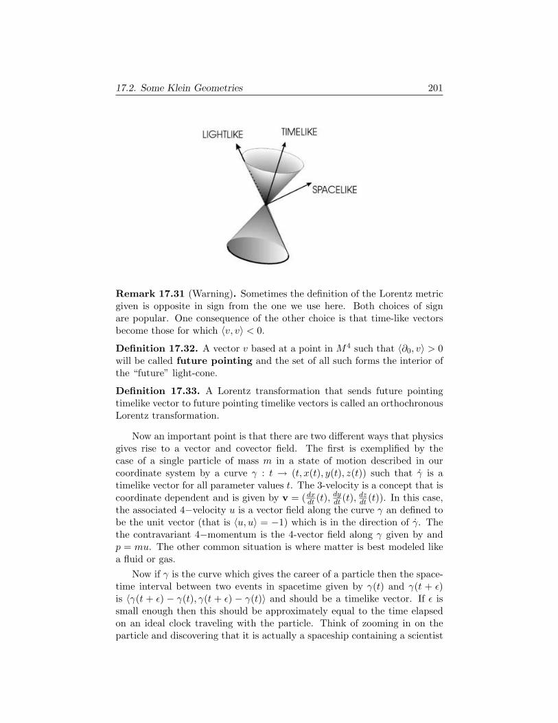
17.2. Some Klein Geometries 201
Remark 17.31 (Warning). Sometimes the definition of the Lorentz metricgiven is opposite in sign from the one we use here. Both choices of signare popular. One consequence of the other choice is that time-like vectorsbecome those for which 〈v, v〉 < 0.
Definition 17.32. A vector v based at a point in M4 such that 〈∂0, v〉 > 0will be called future pointing and the set of all such forms the interior ofthe “future” light-cone.
Definition 17.33. A Lorentz transformation that sends future pointingtimelike vector to future pointing timelike vectors is called an orthochronousLorentz transformation.
Now an important point is that there are two different ways that physicsgives rise to a vector and covector field. The first is exemplified by thecase of a single particle of mass m in a state of motion described in ourcoordinate system by a curve γ : t → (t, x(t), y(t), z(t)) such that γ is atimelike vector for all parameter values t. The 3-velocity is a concept that iscoordinate dependent and is given by v = (dx
dt (t),dydt (t),
dzdt (t)). In this case,
the associated 4−velocity u is a vector field along the curve γ an defined tobe the unit vector (that is 〈u, u〉 = −1) which is in the direction of γ. Thethe contravariant 4−momentum is the 4-vector field along γ given by andp = mu. The other common situation is where matter is best modeled likea fluid or gas.
Now if γ is the curve which gives the career of a particle then the space-time interval between two events in spacetime given by γ(t) and γ(t + ε)is 〈γ(t + ε) − γ(t), γ(t + ε) − γ(t)〉 and should be a timelike vector. If ε issmall enough then this should be approximately equal to the time elapsedon an ideal clock traveling with the particle. Think of zooming in on theparticle and discovering that it is actually a spaceship containing a scientist
202 17. Geometries
and his equipment (including say a very accurate atomic clock).The actualtime that will be observed by the scientist while traveling from significantlyseparated points along her career, say γ(t1) and γ(t) with t > t1 will begiven by
τ(t) =∫ t
t1
|〈γ, γ〉| dt
Standard arguments with change of variables show that the result is indepen-dent of a reparameterization. It is also independent of the choice of Lorentzcoordinates. We have skipped the physics that motivates the interpretationof the above integral as an elapsed time but we can render it plausible byobserving that if γ is a straight line t 7→ (t, x1 + v1t, x2 + v2t, x3 + v3t) whichrepresents a uniform motion at constant speed then by a change to a newLorentz coordinate system and a change of parameter the path will be de-scribed simply by t → (t, 0, 0, 0). The scientist is at rest in her own Lorentzframe. Now the integral reads τ(t) =
∫ t0 1 dt = t. For any timelike curve γ
the quantity τ(t) =∫ tt1|〈γ, γ〉|1/2 dt is called the proper time of the curve
from γ(t1) to γ(t).The famous twins paradox is not really a true paradox since an adequate
explanation is available and the counter-intuitive aspects of the story areactually physically correct. In short the story goes as follows. Joe’s twinBill leaves in a spaceship and travels at say 98% of the speed of light to adistant star and then returns to earth after 100 years of earth time. Letuse make two simplifying assumptions which will not change the validityof the discussion. The first is that the earth, contrary to fact, is at rest insome inertial coordinate system (replace the earth by a space station in deepspace if you like). The second assumption is that Joe’s twin Bill travels atconstant velocity on the forward and return trip. This entails an unrealisticinstant deceleration and acceleration at the star; the turn around but theessential result is the same if we make this part more realistic. Measuringtime in the units where c = 1, the first half of Bill’s trip is given (t, .98t) andsecond half is given by (t,−.98t). Of course, this entails that in the earthframe the distance to the star is .98 lightyears
year × 100 years = 98 light-years.Using a coordinate system fixed relative to the earth we calculate the propertime experienced by Bill:
∫ 100
0|〈γ, γ〉| dt =
∫ 50
0
√|−1 + (.98)2|dt +
∫ 50
0
√|−1 + (−.98)2|dt
= 2× 9. 949 9 = 19. 900
Bill is 19.9 years older when we returns to earth. On the other hand, Joe’shas aged 100 years! One may wonder if there is not a problem here since onemight argue that from Joe’s point of view it was the earth that travelled away
17.2. Some Klein Geometries 203
from him and then returned. This is the paradox but it is quickly resolvedonce it is pointed out that the is not symmetry between Joe’s and Bill’ssituation. In order to return to earth Bill had to turn around which entailan acceleration and more importantly prevented a Bill from being stationarywith respect to any single Lorentz frame. Joe, on the other hand, has beenat rest in a single Lorentz frame the whole time. The age difference effectis real and a scaled down version of such an experiment involving atomicclocks put in relative motion has been carried out and the effect measured.
17.2.6. Hyperbolic Geometry. We have looked at affine spaces, Eu-clidean spaces, Minkowski space and Galilean spacetime. Each of thesehas an associated group and in each case straight lines are maps to straightlines. In a more general context the analogue of straight lines are calledgeodesics a topic we will eventually take up in depth. The notion of dis-tance makes sense in a Euclidean space essentially because each tangentspace is an inner product space. Now each tangent space of En is of theform p×Rn for some point p. This is the set of tangent vectors at p. If wechoose an orthonormal basis for Rn, say e1, ..., en then we get a correspond-ing orthonormal basis in each tangent space which we denote by e1,p, ..., en,p
and where ei,p := (p, ei) for i = 1, 2, ..., n. With respect to this basis in thetangent space the matrix which represents the inner product is the identitymatrix I = (δij). This is true uniformly for each choice of p. One possiblegeneralization is to let the matrix vary with p. This idea eventually leadsto Riemannian geometry. We can give an important example right now.We have already seen that the subgroup SL(2,R) of the group SL(2,C) alsoacts on the complex plane and in fact fixes the upper half plane C+. Ineach tangent space of the upper half plane we may put an inner product asfollows. If vp = (p, v) and wp = (p, w) are in the tangent space of p then theinner product is
〈vp, wp〉 :=v1w1 + v2w2
y2
where p = (x, y) ∼ x + iy and v = (v1, v2), w = (w1, w2). In this context,the assignment of an inner product the tangent space at each point is calleda metric. We are identifying R2 with C. Now the length of a curve γ : t 7→(x(t), y(t)) defined on [a, b] and with image in the upper half-plane is givenby
∫ b
a‖γ(t)‖ dt =
∫ b
a
(x(t)2 + y(t)2
y(t)2
)1/2
dt.
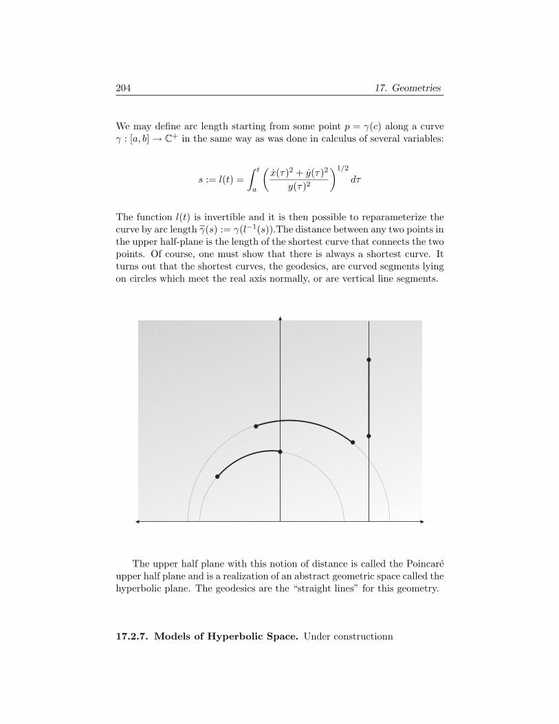
204 17. Geometries
We may define arc length starting from some point p = γ(c) along a curveγ : [a, b] → C+ in the same way as was done in calculus of several variables:
s := l(t) =∫ t
a
(x(τ)2 + y(τ)2
y(τ)2
)1/2
dτ
The function l(t) is invertible and it is then possible to reparameterize thecurve by arc length γ(s) := γ(l−1(s)).The distance between any two points inthe upper half-plane is the length of the shortest curve that connects the twopoints. Of course, one must show that there is always a shortest curve. Itturns out that the shortest curves, the geodesics, are curved segments lyingon circles which meet the real axis normally, or are vertical line segments.
The upper half plane with this notion of distance is called the Poincareupper half plane and is a realization of an abstract geometric space called thehyperbolic plane. The geodesics are the “straight lines” for this geometry.
17.2.7. Models of Hyperbolic Space. Under constructionn
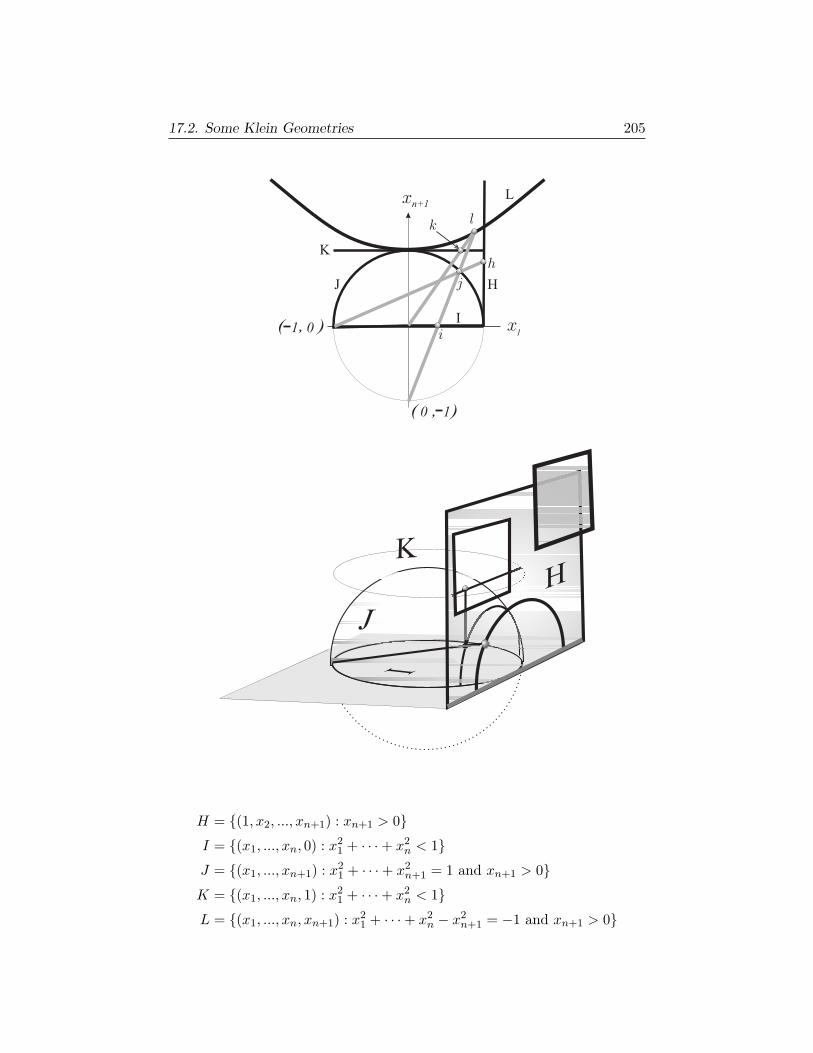
17.2. Some Klein Geometries 205
j
i
k l
h
( , )
( , )0
0
1
1
x
x1
n+1
I
J
K
L
H
H
I
J
K
H = (1, x2, ..., xn+1) : xn+1 > 0I = (x1, ..., xn, 0) : x2
1 + · · ·+ x2n < 1
J = (x1, ..., xn+1) : x21 + · · ·+ x2
n+1 = 1 and xn+1 > 0K = (x1, ..., xn, 1) : x2
1 + · · ·+ x2n < 1
L = (x1, ..., xn, xn+1) : x21 + · · ·+ x2
n − x2n+1 = −1 and xn+1 > 0
206 17. Geometries
α : J → H; (x1, ..., xn+1) 7→ (1, 2x2/(x1 + 1), ..., 2xn+1/(x1 + 1))
β : J → I; (x1, ..., xn+1) 7→ (x1/(xn+1 + 1), ..., xn/(xn+1 + 1), 0)
γ : K → J ; (x1, ..., xn, 1) 7→ (x1, ..., xn,√
1− x21 − · · · − x2
n)
δ : L → J ; (x1, ..., xn+1) 7→ (x1/xn+1, ..., xn/xn+1, 1/xn+1)
The map a is stereographic projection with focal point at (−1, 0, ..., 0)and maps j to h in the diagrams. The map β is a stereographic projectionwith focal point at (0, ..., 0,−1) and maps j to i in the diagrams. The mapγ is vertical orthogonal projection and maps k to j in the diagrams. Themap δ is stereographic projection with focal point at (0, ..., 0,−1) as beforebut this time projecting onto the hyperboloid L.
ds2H =
dx22 + · · ·+ dx2
n+1
x2n+1
;
ds2I = 4
dx21 + · · ·+ dx2
n(1− x2
1 − · · · − x2n
)2 ;
ds2J =
dx21 + · · ·+ dx2
n
x2n+1
ds2K =
dx21 + · · ·+ dx2
n
1− x21 − · · · − x2
n
+(x1dx1 + · · ·+ xndxn)2(
1− x21 − · · · − x2
n
)2
dx2L = dx2
1 + · · ·+ dx2n − dx2
n+1
To get a hint of the kind of things to come, notice that we can have twogeodesics which start at nearby points and start of in the same directionand yet the distance between corresponding points increases. In some sense,the geometry acts like a force which (in this case) repels nearby geodesics.The specific invariant responsible is the curvature. Curvature is a notionthat has a generalization to a much larger context and we will see thatthe identification of curvature with a force field is something that happensin both Einstein’s general theory of relativity and also in gauge theoreticparticle physics. One of the goals of this book is to explore this connectionbetween force and geometry.
Another simple example of curvature acting as a force is the following.Imaging that the planet was completely spherical with a smooth surface.Now imagine the people a few miles apart but both on the equator. Giveeach person a pair of roller skates and once they have them on give them asimultaneous push toward the north. Notice that they start out with parallelmotion. Since they will eventually meet at the north pole the distance
17.2. Some Klein Geometries 207
between them must be shrinking. What is pulling them together. Regardlessof whether one wants to call the cause of their coming together a force ornot, it is clear that it is the curvature of the earth that is responsible.Readers familiar with the basic idea behind General Relativity will knowthat according to that theory, the “force” of gravity is due to the curvedshape of 4-dimensional spacetime. The origin of the curvature is said to bedue to the distribution of mass and energy in space.
17.2.8. The Mobius Group. Let C+∞ denote the set C ∪ ∞. Thetopology we provide C+∞ is generated by the open subsets of C togetherwith sets of the form O∪∞ where O is the compliment of a compact subsetof C. This is the 1-point compactification of C. Topologically, C+∞ isjust the sphere S2.
Now consider the group SL(2,C) consisting of all invertible 2×2 complexmatrices with determinant 1. We have an action of SL(2,C) on C+∞ givenby (
a bc d
)· z =
az + b
cz + d.
For any fixed A ∈ SL(2,C) them map z 7→ A · z is a homeomorphism (andmuch more as we shall eventually see). Notice that this is not the standard
action of SL(2,C) on C2 by multiplication[
z1
z2
]7→ A
[z1
z2
]but there is
a relationship between the two actions. Namely, let[w1
w2
]=
(a bc d
)[z1
z2
]
and define z = z1/z2 and w = w1/w1. Then w = A · z = az+bcz+d . The two
component vectors[
z1
z2
]are sometimes called spinors in physics.
Notice is that for any A ∈ SL(2,C) the homeomorphisms z 7→ A · z andz 7→ (−A) · z are actually equal. Thus group theoretically, the set of alldistinct transformations obtained in this way is really the quotient groupSL(2,C)/I,−I and this is called the Mobius group or group of Mobiustransformations.
There is quite a bit of geometry hiding in the group SL(2,C) and we willeventually discover a relationship between SL(2,C) and the Lorentz group.
When we add the notion of time into the picture we are studying spacesof “events” rather than “literal” geometric points. On the other hand, thespaces of evens might be considered to have a geometry of sorts and soin that sense the events are indeed points. An approach similar to howwe handle Euclidean space will allow us to let spacetime be modeled by aCartesian space R4; we find a family of coordinates related to the standard
208 17. Geometries
coordinates by the action of a group. Of course, in actual physics, the usualcase is where space is 3-dimensional and spacetime is 4−dimensional so letsrestrict attention this case. But what is the right group? What is theright geometry? We now give two answers to this question. The first onecorresponds to intuition quite well and is implicit in the way physics wasdone before the advent of special relativity. The idea is that there is a globalmeasure of time that applies equally well to all points of 3−dimensional spaceand it is unique up to an affine change of parameter t 7→ t′ = at + b. Theaffine change of parameter corresponds to a change in units.
Bibliography
[Arm] M. A. Armstrong, Basic Topology, Springer-Verlag, (1983).
[At] M. F. Atiyah, K-Theory, W.A.Benjamin, (1967).
[A-M-R] R. Abraham, J.E. Marsden,, and T. Ratiu, Manifolds, tensor analysis, andapplications, Addison Wesley, Reading, (1983).
[Arn] V.I. Arnold, Mathematical methods of classical mechanics, Graduate Texts inMath. 60, Springer-Verlag, New York, 2nd edition (1989).
[BaMu] John Baez and Javier P. Muniain, Gauge Fields, Knots and Gravity, WorldScientific, (1994).
[Be] Arthur L. Besse, Einstein Manifolds, Classics in Mathematics, Springer,(1987).
[BishCr] R. L. Bishop and R. J. Crittenden, Geometry of Manifolds, NewYork:Academic Press, (1964).
[Bo-Tu] R. Bott and L. Tu, Differential Forms in Algebraic Topology, Springer-VerlagGTM 82, (1982).
[Bre] G. Bredon, Topology and Geometry, Springer-Verlag GTM 139, (1993).
[BrCl] F. Brickell and R. Clark, Differentiable Manifolds; An Introduction, Van Nos-tran Rienhold, (1970).
[Bro-Jan] Th. Brocker and K. Janich, Introduction to Differential Topology, CambridgeUniversity Press, (1982).
[Brou] L.E.J. Brouwer, “ Uber Abbildung von Mannigfaltigkeiten,” MathematischeAnnalen 71 (1912) 97-115.
[Chavel] I. Chavel, Eigenvalues in Riemannian Geometry, Orlando: Academic Press,(1984).
[C-E] J. Cheeger and D. Ebin, Comparison Theorems in Riemannian Geometry,Amsterdam: North-Holland, (1975).
[Cheng] S.Y. Cheng, Eigenvalue Comparison Theorems and its Geometric Applica-tions Math. Z. 143, 289–297, (1975).
[Clark] C.J.S. Clark, On the Global isometric embedding of pseudo-Riemannian man-ifolds, Proc. Roy. Soc. A314 (1970) 417-428
209
210 Bibliography
[Dar] R. W. R. Darling, Differential Forms and Connections, Cambridge UniversityPress, (1994)
[Dieu] J. Dieudonn´e, A History of Algebraic and Differential Topology 1900-1960,Birkhauser,(1989).
[Dod-Pos] C.T.J. Dodson and T. Poston, Tensor Geometry: The Geometric Viewpointand Its Uses, Springer-Verlag (2000).
[Dol] A. Dold, Lectures on Algebraic Topology, Springer-Verlag, (1980).
[Donaldson] S. Donaldson, An application of Gauge theory to the Topology of 4-manifolds,J. Diff. Geo. 18 (1983), 269-316.
[Dug] J. Dugundji, Topology, Allyn & Bacon, (1966).
[Eil-St] S. Eilenberg and N. Steenrod, Foundations of Algebraic Topology, PrincetonUniv. Press, (1952).
[Fen] R. Fenn, Techniques of Geometric Topology, Cambridge Univ. Press, (1983).
[Freedman] M. Freedman, The Topology of Four Dimensional Manifolds, J. Diff. Geo. 17(1982) 357-454.
[Fr-Qu] M. Freedman and F. Quinn, Topology of 4-Manifolds, Princeton Univ. Press,(1990).
[Fult] W. Fulton, Algebraic Topology: A First Course, Springer-Verlag, (1995).
[G2] V. Guillemin, , and S. Sternberg, Symplectic Techniques in Physics, Cam-bridge Univ. Press, Cambridge, (1984).
[Gu-Hu-We] K. Guruprasad, J. Huebschmann, L. Jeffrey, and A. Weinstein, Group sys-tems, groupoids, and moduli spaces of parabolic bundles, Duke Math. J. 89(1997), 377-412.
[Gray] B. Gray, Homotopy Theory, Academic Press, (1975).
[Gre-Hrp] M. Greenberg and J. Harper, Algebraic Topology: A First Course, Addison-Wesley, (1981).
[Grom] M. Gromov, “Convex sets and Kahler manifolds” in Advances in differentialgeometry and topology, World Sci. Publ., Teaneck, NJ ,1990, 1-38.
[Helg] S. Helgason, Differential Geometry, Lie Groups and Symmetric Spaces, Amer.Math. Soc., 2001.
[Hicks] Noel J. Hicks, Notes on Differential Geometry, D. Van Nostrand CompanyInc, (1965).
[Hilt1] P. J. Hilton, An Introduction to Homotopy Theory, Cambridge UniversityPress, (1953).
[Hilt2] P. J. Hilton and U. Stammbach, A Course in Homological Algebra, Springer-Verlag, (1970).
[Hus] D. Husemoller, Fibre Bundles, McGraw-Hill, (1966) (later editions bySpringer-Verlag).
[Kirb-Seib] R. Kirby and L. Siebenmann, Foundational Essays on Topological Manifolds,Smoothings, and Triangulations, Ann. of Math.Studies 88, (1977).
[Klein] Felix Klein, Gesammelte Abhandlungen, Vol I, Springer, Berlin, (1971).
[Kob] S. Kobayashi, On Conjugate and Cut Loci in Global Differential Geometry,M.A.A. Studies in Maths, Vol. 27, S.S Chern Editor, Prentice Hall (1989)
[K-N] S. Kobayashi and K. Nomizu, Foundations of Differential Geometry. I, II, J.Wiley Interscience, (1963), (1969).
Bibliography 211
[L1] S. Lang, Fundamentals of Differential Geometry, Springer-Verlag GTM vol191
[L2] S. Lang, Algebra, Springer-Verlag GTM vol 211
[L-M] H. Lawson and M. Michelsohn, Spin geometry, Princeton University Press,Princeton, (1989).
[Lee, Jeff] Jeffrey M Lee, Online Supplement to the present text, Internet:http://webpages.acs.ttu.edu/jlee/Supp.pdf
[Lee, John] John Lee, Introduction to Smooth Manifolds, Springer-Verlag GTM vol 218(2002).
[L-R] David Lovelock and Hanno Rund, Tensors, Differential forms, and VariationalPrinciples, Dover Publications, New York (1989).
[Madsen] Id Madsen and Jørgen Tornehave, From Calculus to Cohomology, CambridgeUniversity Press (1997).
[Matsu] Y. Matsushima, Differentiable Manifolds, Marcel Dekker, New York, 1972.
[M-T-W] C. Misner, J. Wheeler, and K. Thorne, Gravitation, Freeman, (1974)
[Mil] J. Milnor, Morse Theory, Annals of Mathematics Studies 51, Princeton U.Press, Princeton, (1963).
[MacL] S. MacLane, Categories for the Working Mathematician, Springer-VerlagGTM 5, (1971).
[Mass] W. Massey, Algebraic Topology: An Introduction, Harcourt, Brace & World,(1967) (reprinted by Springer-Verlag).
[Mass2] W. Massey, A Basic Course in Algebraic Topology, Springer-Verlag, (1993).
[Maun] C. R. F. Maunder, Algebraic Topology, Cambridge Univ. Press, (1980)(reprinted by Dover Publications).
[Mich] P. Michor, Topics in Differential Geometry, Graduate Studies in Mathemat-ics, v.93, (2008)
[Miln1] J. Milnor, Topology from the Differentiable Viewpoint, Univ. Press of Virginia,(1965).
[Mil-St] J. Milnor and J. Stasheff, Characteristic Classes, Ann. of Math. Studies 76,(1974).
[Molino] P. Molino, Riemannian foliations, Progress in Mathematics, Boston:Birkhauser, (1988).
[My-St] S. B. Myers, N. E. Steenrod, The group of isometries of a Riemannian man-ifold. Annals of Mathematics, Vol. 40, No. 2, (1939).
[ON1] B. O’Neill, Semi-Riemannian Geometry, Academic Press, New York, (1983).
[ON2] B. O’Neill, Elementary differential geometry, Academic Press, (1997).
[Pa] Richard, Palais, Natural Operations on Differential Forms, Trans. Amer.Math. Soc. (1959), pp 125-141
[Pa2] Richard, Palais, A Modern Course on Curves and Surfaces, Online Book athttp://www.math.uci.edu/˜cterng/NotesByPalais.pdf.
[Pen] Roger Penrose, The Road to Reality, Alfred A. Knopf, New York, (2005).
[Pe] Peter Peterson, Riemannian Geometry, Springer-Verlag (1991).
[Poor] Walter Poor, Differential Geometric Structures, Mcgraw Hill, (1981).
[Nash1] John Nash, C1-isometric imbeddings”, Annals of Mathematics, 60 (1954), pp383-396.
212 Bibliography
[Nash2] John Nash, The imbedding problem for Riemannian manifolds, Annals ofMathematics, 63 (1956), pp 20-63.
[Roe] J. Roe, Elliptic Operators, Topology and Asymptotic methods, Longman,(1988).
[Ros] W. Rossmann, Lie Groups: An Introduction through Linear Groups, OxfordUniversity Press (2002).
[Shrp] R. Sharpe, Differential Geometry; Cartan’s Generalization of Klein’s Erlan-gen Program, Springer-Verlag (1997).
[Span] Edwin H. Spanier, Algebraic Topology, Springer-Verlag, (1966).
[Spv] M. Spivak, A Comprehensive Introduction to Differential Geometry, (5 vol-umes) Publish or Perish Press, (1979).
[St] N. Steenrod. Topology of fiber bundles, Princeton University Press, (1951).
[Stern] Shlomo Sternberg, Lectures on Differential Geometry, Prentice Hall (1964).
[Tond] Ph. Tondeur, Foliations on Riemannian manifolds, New York: Springer Ver-lag, (1988).
[Tond2] Ph. Tondeur, Geometry of Foliations, Monographs in Mathematics, vol. 90,Basel: Birkhauser, (1997).
[Wal] Gerard Walschap, Metric Structures in Differential Geometry, Springer-Verlag, (2004).
[War] Frank Warner,. Foundations of Differentiable Manifolds and Lie Groups,Springer-Verlag, (1983).
[Wh] John A. Wheeler, A Journey into Gravity and Spacetime, Scientific AmericanLibrary, A division of HPHLP, New York (1990).
[We1] A. Weinstein, Lectures on Symplectic Manifolds, Regional conference seriesin mathematics 29, Amer. Math. Soc.,Providence, (1977).
Index
admissible chart, 69
almost complex manifold, 140
almost symplectic, 153
antiholomorphic, 139
atlas, 69
canonical 1-form, 161
Cauchy-Bochner integral, 30
chain rule, 33
chart, 69
co-symplectic structure, 172
coadjoint action, 153
coisotropic, 172
complex manifold, 140
coordinates, 70
Darboux’s theorem, 157
derivation, 95
derivative, 29
diffeomorphism, 29
differentiable structure, 69
dimension, 70
evolution operator, 76
fiber derivative, 164
general linear group, 26
germ of section, 102
Grassmannian, 141
half rank, 150
Hamiltonian action, 169
Hamiltonian vector field, 160
holomorphic, 139
implicit napping theorem, 41
infinitesimal automorphism, 122
integral curve, 75
Kahler manifold, 155
Lagrangian subspace, 150
leaf, 121
Levi decomposition, 94
Lie algebra action, 168
local diffeomorphism, 36
locally Hamiltonian, 161
model space, 67
momentum map, 169
multilinear, 27
musical isomophisms, symplectic, 156
phase space, 161
Poisson Bracket, 171
Poisson bracket, 159
Poisson structure, 172
principal bundle, 127
product rule, 35
regular Lagrangian, 164
Riemann sphere, 141
Riemann surface, 142
rigid body, 166
Sard’s theorem, 71
sheaf of germs, 102
split, 25
stable family, 121
strongly Hamiltonian, 170
suspension, 75
213

214 Index
symplectic action, 168, 169symplectic form, 152symplectic group, 150symplectic manifold, 152symplectic subspace, 150symplectic vector field, 160symplectic vector space, 149