Macalester CollegeDigitalCommons@Macalester College

Honors Projects Economics Department

5-5-2008

Subsistence Theory in the U.S. Context: A Cross-Sectional Labor Supply EstimateJennifer Bendewaldjbendewald@macalester.edu

Follow this and additional works at: http://digitalcommons.macalester.edu/economics_honors_projects

This Article is brought to you for free and open access by the Economics Department at DigitalCommons@Macalester College. It has been acceptedfor inclusion in Honors Projects by an authorized administrator of DigitalCommons@Macalester College. For more information, please contactscholarpub@macalester.edu.

Recommended CitationBendewald, Jennifer, "Subsistence Theory in the U.S. Context: A Cross-Sectional Labor Supply Estimate" (2008). Honors Projects.Paper 7.http://digitalcommons.macalester.edu/economics_honors_projects/7

Subsistence Theory in the U.S. Context:

A Cross-Sectional Labor Supply Estimate

Jennifer Bendewald Honors Thesis

Economics Department Advisor: Raymond Robertson

5/5/08

Abstract:

Subsistence theory predicts the distress sale of labor at very low wages, such that the income effect dominates not only at high wages (as is relatively established) but also below a ‘subsistence wage’. This theory has been developed and tested in the context of mainly agricultural economies, but more recent theoretical work has suggested its applicability in industrialized economies, where it has not yet been tested. Some previous studies of labor supply in the context of the United States have experimented with flexible functional forms, noting that the canonical model makes no a priori predictions as to its shape. However, little attention is given to the slope changes themselves, which are of prime importance in subsistence theory. This paper uses a unique method of pinpointing endogenous slope changes in the estimated labor supply response, finding the ‘subsistence wage’ to be $6.60/hr ($8.39 in 2008 dollars) using 2000 Census data. This is not only inherently interesting but also important for minimum wage policy, because setting the minimum wage up to this level would not increase unemployment.

2

Introduction

While econometric techniques in labor economics have become very sophisticated, advances in

the theoretical understanding of the labor supply decisions in low-income households have

lagged behind. The canonical model, based on work and leisure preferences regardless of

minimal consumption requirements, implies a set of choices that are probably not available to

low-income workers—including those in relatively rich nations such as the United States.

Namely, workers who earn a wage that just barely allows for subsistence are fundamentally

different from middle class workers—in terms of their labor supply response—because a

minimum consumption constraint generally becomes binding only at low wages. Where this

constraint is binding, the income effect must dominate the substitution effect. Assuming workers

at each income level have—or can have—the same response to wage changes can lead to

misleading policy analyses.1 Subsistence theory offers a richer explanation of the choices and

constraints facing poor workers, and yet is rarely seen in the context of industrialized economies.

Low-income workers in America undoubtedly face circumstances different from those in

developing economies, due to the better-established network of government and nonprofit aid

organizations in the United States. However, there are fundamental similarities in the two cases,

especially when those aid organizations are unable to meet the demand for assistance. According

to one survey of U.S. cities, half of all those seeking emergency food assistance are in families

with children, and nearly a quarter of aid requests go unmet.2 Similar evidence of the precarious

financial situation and the so-called “time crunch” of some households in the United States is

given by Mishel et al. (2003) and Burton and Phipps (2007). The complex—and imperfect—

1 For instance, the highly regarded research in Eissa (1995) uses a differences-in-differences approach to the effects of a tax policy that assumes workers at different income levels have the same labor supply elasticity. To her credit, the author acknowledges this weakness. 2 The current U.S. Hunger Survey, commissioned each year by the Council of Mayors, reports on food assistance programs in 23 cities.

3

social safety net affects labor supply decisions in ways that have not been decisively quantified,

but the evidence suggests that an analysis of U.S. labor supply using subsistence wage theory

would be fruitful.

Allowing slope changes in labor supply estimations has become standard in the literature,

given that the canonical model offers no a priori reason to believe the labor supply curve is

linear. However, precisely because of the standard model’s agnosticism, explaining why the

income or substitution effect dominates is seen as unnecessary. Subsistence theory, with its

easily testable prediction of a negative wage response at low wages, offers an explanation of the

shape of the labor supply curve that is both elegant and policy-relevant.

Subsistence theory, in the context of aggregate labor supply, has implications for

minimum wage policies (Dessing (2002, 2004)). The predicted turning point from negative to

positive wage response marks an endogenous level of subsistence (following Sharif (2003)),

below which point individuals must supply ever more labor to the market to maintain a minimum

amount of consumption. This is the so called ‘distress sale of labor’ phenomenon. Raising the

minimum wage to this point could theoretically reduce unemployment by restricting excess

supply, a result consistent with the findings reviewed in Card and Krueger (1995). Using 2000

Census data, I estimate an endogenous subsistence wage for married-couple households at $6.58/

hr, a finding with important implications but also considerable caveats.

The rest of the paper is organized as follows: section two provides a review of the

relevant literature, section three develops subsistence theory and its effect on the full labor

supply schedule, section four describes the Census data used for this study, section five provides

estimation technique and results, and section six concludes with policy implications.

4

Literature Review

The canonical model of labor supply, conceptually akin to the model of consumer demand, is the

most common and most enduring basis for economic analyses of the work decision. In this

framework, work hours are usually modeled as a function of the individual’s available wage rate

and of any income received independent of the work decision (inheritance, for example, or

interest income). Indeed, this model is the foundation for more than 30 years of labor economics,

and this longevity is testament both to the strength of its framework and to its adaptability

(Killingsworth 1983). The first two distinguishable generations of research have been amply

reviewed (Killingsworth (1983); Pencavel (1986)), as have developments in the field since then

(Blundell and MaCurdy (1999) and Moffitt (1999)). Current research has moved toward using

natural experiments to measure labor supply elasticity, in which, theoretically, an exogenous

shock to the wage cases measurable changes in hours worked. This technique is favored because

it avoids most of the drawbacks to cross-sectional estimates.3 While great strides were made both

in econometric techniques and in exploring complications to the model, one relatively

overlooked issue has been the fundamentally unique situation of the working poor, whose

consumption level often hovers at a barely-sustainable rate (Sharif 2000).

Subsistence theory has its roots in analyses of developing or agricultural economies, and

econometric studies that explicitly test the theory are in this context (reviewed in Sharif (2000))4.

The theory, based on the notion that workers basically have only their labor to sell in exchange

for the level of consumption necessary for survival, has been substantiated by a wealth of

empirical evidence in these economies. Its most powerful addition to the standard theory is the

3 Panel data is the optimal source for labor research to estimate how individuals—as opposed to the representative worker—responds to wage changes. 4 The concept of a subsistence wage—and the corresponding forward-falling labor supply curve below this wage—is explained by nutritionist, target income, and distress sale of labor theories, and I will refer to these theories using the umbrella term ‘subsistence theory’.

5

prediction of slope direction, which is commonly seen as a solely empirical question. Because of

this, the theory lends itself well to hypothesis-testing. When this theory surfaces in the U.S.

context, it is used most often as a post-estimation explanation of negative wage elasticities rather

than the theoretical basis of the study (examples are Leuthold (1968) and Dunn (1978)). An

important exception to this is Barzel and McDonald (1973), who develop a model for the U.S.

context that predicts an initial negative slope in the labor supply curve if the value of assets does

not cover a minimal consumption level. They provide evidence for their theory using U.S. data,

aggregated by year between 1901 and 1961, showing that years with the lowest wages also

exhibited the most hours worked. Sharif notes the uncertainty as to whether this theory is still

meaningful in the context of industrialized economies, where, in most cases, institutions exist to

ensure a minimally sufficient level of consumption, sometimes regardless of hours worked.

Despite the shortage of explicit hypothesis testing in the context of industrialized

economies, many of the empirical studies in the United States and United Kingdom do provide

results of negative elasticities among low-income workers consistent with these theories. In

contrast to Leuthold (1968) and Dunn (1978), Hill (1973) and Hurd (1976) offer no theoretical

‘story’ to explain their evidence of negative elasticity at low wages. However, they are notable

for allowing slope changes in their estimates. Hill (1973) estimates the labor supply in 1966 of

poor heads of households using the 1967 Survey of Economic Opportunity (SEO), including a

quadratic term in the wage variable, and finds a uniformly negative elasticity among whites (that

is, the quadratic term is insignificant) and a ‘backward bend’ turning point at $1.14/hr ($7.45 in

2008 dollars) among blacks, below which elasticity is positive. Hurd (1976) is the only existing

study, to this author’s knowledge, which estimates a labor supply curve piecewise linear in the

wage rate, the form utilized in this study. Also using data from the 1967 SEO, these estimates

6

indicate negative elasticities among both men and women for the lowest and highest own wage

ranges5, with the middle range positive: in other words, an inverted-S-shaped curve. It may be

helpful to note that, because the standard theory of labor supply offers no prediction as to

whether the income or substitution effect will dominate at any given wage rate, most researchers

understandably felt no need to explain their findings in a behavioral context. Indeed, Hurd

explains his use of the piecewise functional form on the grounds that welfare analysis, the focus

of his study, requires the best fit over all of the data. Likewise in testing the predictions of

subsistence theory, this functional form is a natural choice.

Subsistence theory makes a powerful addition to the canonical model in predicting that

the labor supply curve will exhibit a negative slope at low wages. The standard model makes no

a priori prediction as to the slope or even the form of the aggregate labor supply function, but it

is often assumed that the income effect will rise with the wage, tending to dominate at the

highest wages: the so-called backward-bending labor supply curve6. A forward-falling segment

at low wages would complete an S-shaped labor supply curve, as put forth in Sharif (2000).

Sharif (2003) explores the theoretic importance of the subsistence wage to behavioral labor

economics, arguing that the slope change from negative to positive represents an endogenous

level of sustainability. However, the implications of this theory for labor market regulation were

first explored in Dessing (2002, 2004). In the only empirical work on the S-shaped labor supply

curve to date, Dessing develops and tests a model of household labor supply in the contexts of

Indonesia and Costa Rica, respectively, finding evidence for the theory in both cases. In light of

this evidence, she provides a theoretical justification for setting the minimum wage equal to the

5 Among women, elasticity is negative for wages between $0.50 and $1.00 ($3.27—6.53 in 2008 dollars) and for those between $2.50 and $4.50 ($16.33—29.40). Among men, the forward-falling range is the same and the backward bend comes between $4.50 and $20 ($29.40—$130.67). 6 This is the form appearing in most textbooks when introducing labor supply, for instance those cited in Barzel and McDonald (1973) and, more recently, Mankiw (2004) and McConnell et al. (2006).

7

subsistence wage, to prevent a “race to the bottom”. In more formal terms, market equilibria

below the subsistence wage are unstable: wage decreases will spur labor surpluses, which in turn

will drive down wages yet more. Employers in this case are said to race each other to offer the

lowest wages, cutting costs and yet facing a surplus of available labor.

Pinpointing the wage at which the slope becomes positive is clearly essential in

understanding the parameters of this phenomenon—and in giving precise policy

recommendations—yet even in the subsistence wage literature, this is not undertaken (Anderson

(2004)). In this study, I will directly extend the empirical work of Dessing (2002, 2004) both by

testing this theory in the U.S. context and by explicitly estimating the subsistence wage. This

paper also adds to the literature more generally by applying a technique of determining

endogenous breaks in a trend to cross-sectional data.

Theory

I. Model of Labor Supply

The canonical model of labor supply is similar to that of consumer demand, in which the

commodity bought and sold is time, in the form of leisure and market work, respectively. In this

optimization problem, individuals’ utility is assumed to be a function of the consumption of

goods and leisure (defined as time not spent working):

(1.1) u = u(C, L; x)

where x is the exogenous set of an individual’s unobserved preferences, graphically represented

by the indifference curves. Individuals are assumed to maximize utility subject to both a time

constraint and a budget constraint. Total available time, T, is the sum of hours spent working, H,

and hours taken for leisure:

8

(1.2) T = H + L

The budget constraint in this single-period model completely restricts consumption by income.

The dollar amount of consumption is a function of P, the unit price of the bundle of consumption

goods C. The dollar amount of total income includes both wage income, where w is the average

and marginal wage (that is, the budget constraint is linear), and income independent of the labor

supply decision, V:

(1.3) PC = wH +V

This is the most basic model to which subsistence theory adds a minimum consumption

constraint, such that the dollar value of S, the minimum consumption level needed for survival,

must be covered by total income:

(1.4) PS ≤ wH +V

Changes in the wage rate are seen in terms of a substitution effect, in which workers view

leisure as more expensive and work more, and an income effect, in which added wealth means

workers can consume more leisure and work less. The relative magnitudes of the income and

substitution effects determine the slope of the labor supply schedule.

The concept of the reservation wage, defined as the wage at which an individual will

decide to begin supplying labor to the market, captures a key difference between subsistence

wage theories and the canonical model. In the canonical model, individuals will opt out of the

labor force (H = 0) for any wage below their reservation wage. As the wage rate rises above their

reservation wage, workers will supply increasingly more hours of labor. Thus, whether an

individual works is determined primarily by market forces. This has commonly been viewed as

descriptive of married women’s labor supply decision, which is marked by a high value of V in

9

their husbands’ income and, historically, wages lower than men’s. Instead of working in the

labor market, then, the rational choice would be to work in the home.

Including the concept of minimal consumption needs into the model drastically changes

the corner solution: in this theory, an individual will devote all available time to market work at

the lowest possible wage. Specifically, if nonlabor income V does not cover basic needs, an

individual will have to work enough to afford these costs. Moreover, if the wage rate available is

low, that worker will have to work more to get by than if the available wage were higher. The

key difference from the simpler model is that the point of labor market entry is determined by

physical needs (in the form of food, rest, shelter, etc.), rather than by the going wage rate.

The addition of the subsistence model to the classic labor supply curve is best seen in an

illustration of the full labor supply schedule with the subsistence income, Figure 1, explained

below.

10

Figure 1. Family Labor Supply with a Subsistence Income

Total Family Labor

Wage Family time constraint

Subsistence Wage

Reservation Wage

Family labor supply

Primary workers h Secondary workers h

Subsistence frontier

*Adapted from Dessing (2002).

Labor supply below the subsistence wage closely follows the subsistence frontier, defined

as the income which families can earn enough to meet their basic needs of food, shelter, and

physical rest. Income along the subsistence frontier is by definition constant: this is the ‘target

income’ of target income theory. This negative slope along the subsistence income is

fundamentally different from the backward-bending portion of the labor supply curve, because,

as argued in Sharif (2003), these wages entail a ‘restricted freedom of choice’. Simply put, there

is no real choice, given a decrease in the wage below the subsistence wage, between working less

(and not earning enough to subsist) and working more (and maintaining a minimum consumption

11

rate). The income effect is in this case constrained to dominate the substitution effect. The

hypothesized backward-bending portion of the labor supply curve of course entails no such

restriction on choice.

Following Dessing (2002), I focus on family labor supply as the most applicable test of

subsistence theory. Primary workers are assumed to basically work full time, with the variation

in household hours originating in the secondary worker’s labor supply, seen in Figure 1. In a

departure from the literature, the wage rate earned by the householder is considered the

appropriate wage of analysis for the household: the head therefore experiences no cross-

substitution effect and the spouse no own-substitution effect. Dessing justifies this by arguing

that the head of the family is socialized into working full time regardless of his/her wage rate,

and that the spouse will determine his/her hours based not on his/her own wage rate but rather

whether the householder can earn enough, working full time, to support the whole family. Cross-

substitution effects are often assumed to be zero in empirical estimates of family labor supply for

simplicity, but estimates allowing for cross-substitution suggest that women in the United States

are more responsive to their spouses’ wage than the spouses themselves (Blundell and MaCurdy

(1999))7. At least one sensitivity analysis concludes that the inclusion of the wife’s wage or

earnings in the hours equation has no effect on the husband’s wage response (DaVanzo 1973).

The model to be estimated takes the form:

(1.5) H i = β0 + β1 lnWi + β2Y + β3Ni + Xi + ε

7Pertinent to note here is the Census definition of ‘head of household’: it is the individual in whose name the property is owned, rented, or leased (Census 2000). This definition is more helpful in the terms of this study than simply defining the head as the male half of a married couple, precisely because the official property owner/ renter/ leaser is presumably also the primary breadwinner, regardless of gender.

12

where, for family i, H is the total yearly hours worked by the head and the spouse, lnW is the

natural log of the average wage rate of the head, Y is yearly household income independent of

work hours, N is a measure of income needs, X is a vector of demographic control variables.8

Like Hurd (1976), I divide my sample by wage brackets. This allows the coefficients to

vary across the wage spectrum, with the key parameter in testing the predictions of subsistence

theory being the wage response, β1. Unlike Hurd, I estimate endogenous wage brackets to

pinpoint the two major, hypothesized changes in slope. This technique is described in Section II

below.

II. Model of Endogenous Breaks in a Trend

Previous research has experimented with various functional forms in specifying the labor supply

function (important works include Blundell and Meghir (1986) and Stern (1986)), but I approach

the problem of allowing changes in the slope of the labor supply curve using a time series

technique developed to locate endogenous breaks in a trend. This approach allows me both to use

a straightforward specification in the hours equation and to easily pinpoint the location of slope

changes, which is the ultimate goal of this research.

Unit root tests are generally applied to macroeconomic questions, such as whether GDP

follows a ‘random walk’. Early tests (see Vogelsang and Perron (1998) for a review) allowed for

a break in the trend where the break is exogenous. Criticisms of data mining led to the adaptation

of these tests to allow for an endogenous break. It is this development of allowing for an

unknown break that allows me to apply the technique to my question of whether the labor supply

curve is S-shaped as predicted by subsistence theory. As discussed above, subsistence theory

8 The natural log of the wage is used because wages have been found to be log-normally distributed, which becomes important if the wage is used as a dependent variable. Instrumenting the wage to control for endogeneity, a procedure that I use and describe in the results section, is one such case.

13

predicts a negative slope of the labor supply curve at low wages, with the slope becoming

positive as the wage increases to allow for total income greater than this subsistence level. In

other words, a break in the trend of hours worked as the wage increases is implied. Treating my

wage variable as time allows me to estimate the ‘moment’ of this break, or the sustainable wage

rate. The full, inverted-S-shaped labor supply curve of course involves both a break at the

subsistence wage and at the backward-bend, such that we expect two breaks to be revealed.

I use the Additive Outlier (AO) theory developed in Perron and Vogelsang (1998) for this

analysis, which models a sudden break in the trend.9 In their notation:

(1.6) yt = µ0 + βt +θDUt

c + γ DTt

c + zt

where DUtc equals 1 if t is after the break, 0 if otherwise, and DTt

c equals the trend term if t is

after the break, 0 if otherwise. The endogenous break, Tb, is chosen where the t-statistic on the

break parameter γ is highest in absolute value. In the context of my cross sectional study, the

‘trend term’ is the wage rate, and the break parameter γ is most significant at any wage rate

marking a significant change in labor supply elasticity.10 The relevant notation in terms of my

estimated equation (1.5) is:

(1.7) H i =β0 +θDUw +γDWw +β1lnWi +β2Yi +N i +Xi

where DUw equals 1 if the wage rate w is greater than the (unknown) break(s) in the labor supply

function, 0 if otherwise, and DWw is the interaction term (DUw*lnW). This equation is iterated at

increments of 0.1 natural log of the wage. This gives me the t-statistic, t, on γ at each increment,

9 The Innovative Outlier (IO) model depicts an evolutionary break. My choice of the AO model in the exploration of this technique is based on the theory that the subsistence wage will be a relatively clear break. Future research may explore whether the IO model gives similar results. 10 The calculation of t-statistics is of course inherently connected with sample size. My wage data, in contrast to time series data, varies in sample size at each wage rate marking a potential break. To see that

this does not influence the t-statistic on γ, note that it is always calculated over the entire sample size, and does not depend on the number of observations at each wage rate.

14

so that finding the wage rate at the global maximum and minimum of t, which are predicted to

mark both the subsistence wage and the wage marking the backward bend, is straightforward.

Summary Statistics

I use data from the 1% PUMS sample of the 2000 Census for all 50 states plus the District of

Columbia, taken from the IPUMS database (Ruggles 2004). As a preliminary exploration of

whether the predictions of subsistence theory are accurate in the U.S. context, the very large and

representative sample afforded by the Census is a decisive advantage.11 Household type is

restricted to those headed by a married couple due to my theoretical basis, which assumes the

household maximizes utility as one unit. Both the head of household and the spouse must be

between 18 and 65 years old, or in what I assume to be prime working age, and both must be

citizens, to avoid the complications of work restrictions on non-citizens. Finally, I also limit my

sample to households whose heads are wage or salary earners (in other words, are not self-

employed) and who thus face a clearer hourly wage.12 After these limitations, the sample

represents 23.7% of the total Census data set, or 324,178 couples. In all cases, I use the Census

person weights to ensure the sample is representative.13

The ideal data set for an estimation of the labor supply function would include explicit

data on preferences for work, which would correspond to the indifference curve between

consumption and leisure in the simple model. It would also include the marginal wage rate for

workers as well as the potential marginal wage for non-workers. Available data is much less

11 Later research may determine whether other data sets, such as the widely-used Current Population Survey (CPS), substantiate the current research. 12 For an argument that such this limitation entails selection bias, see Gill (1988). He finds self-employment to be positively correlated with education. The limitation to households with non-self-employed heads reduces my sample 12.9%. 13 Person rather than household weights are used because I use individual income data. This is in accordance with the recommendation in the PUMS documentation (Census).

15

complete: the Census in particular is prone to ‘noisy’ wage data and rounded hours data (Angrist

and Krueger (1999)). It also gives only before-tax income, although after-tax income is more

pertinent to the study of labor supply insofar as workers behave according to their take-home

rather than gross wage.14

The Census collects data on several types of income, of which I use two: yearly

individual income from wages and salary and yearly household income. To generate average

wages, I divide wage and salary income by hours worked in the year (which in turn is generated

by multiplying the variables for weeks worked and usual hours worked per week). Household

income is the combined total income, both earned and unearned, of all household members. To

generate my variable for household unearned income, I subtract the earned income of the head

and the spouse from total household income. This captures such income sources as interest,

property, or public assistance income.15 The limitations of Census data for use in labor

economics have been well documented (Killingsworth (1983); Angrist and Krueger (1999)),

including a potentially important bias when researchers must calculate the wage using the

dependent variable (yearly work hours)16. Income variables are based on respondents’ memory—

and willingness to disclose this information—and tend to be underreported in the Census.

Informal work is also not captured by these variables, which probably biases the data on poor

14 Importantly, taxes introduce ‘kinks’ in the budget constraint—more so at low than at moderate wages—and these kinks introduce more complex incentives regarding work behavior than those implied by a single, linear budget constraint. This, too, is cause for caution when interpreting the results of this study. 15 Public assistance is of course directly connected to the work decision, insofar as welfare programs in place by 1999 require recipients to at least actively seek employment. Labeling public assistance as unearned income is therefore not wholly correct, for it affects hours in a more complicated way than either unearned income or the wage rate do, which is beyond the scope of this study. 16 Namely, estimates of labor supply response will be biased downward in the presence of measurement error in the hours variable.

16

workers more than wealthy17. Though the benefits of using a large, representative sample

outweigh the costs of possible ‘noisy’ variables for the purposes of this study, these limitations

of the income variables are potentially large and are reason for caution in interpreting the results

of this study.

Where Dessing (2002) uses assets as a proxy for income needs, this study relies on

housing costs. The Census includes no variable for assets but does include a fairly complete

picture of housing costs, by collecting data on rent, mortgage payments, mobile home fees, and

the costs of electricity, gas, water, and home heating fuels.18

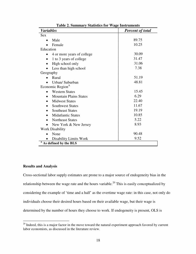
Summary statistics are given in Tables 1 and 2, below.19 The number of observations

refers to households, not individuals. Hours worked by the household exhibits a fair amount of

variation, important in a dependent variable. The average wage is of course heavily skewed to

high values, substantiating the need for log values when using the wage as the dependent

variable.

17 Bartering, undisclosed self-employment, and informal work arrangements are, according to research in other social sciences, quite common strategies among the poor in America (Shipler (2004) and Edin (2001)). 18 Housing costs, to the extent that they are indeed correlated with income, are endogenous and therefore not a consistent predictor of hours. 19 Two-way correlations between the variables are given in Table 6 the Appendix, and give no suggestion of colinearity.

17

Table 1. Summary Statistics for the Household

Variables Mean (Std. Error)

Percent of total

Yearly Household Hours Worked 3556.4 (1168)

--

Average WageA 24.306 (98.67)

--

Yearly Household Nonlabor IncomeB 8256.3 (21040)

--

Housing CostC 5211.8 (4139)

--

Couples with No Children -- 33.91

Couples with One Child -- 24.57

Couples with Two Children -- 27.06

Couples with Three or More Children -- 14.46

White -- 86.66

Black -- 6.89

American Indian or Alaska Native -- 0.79

Chinese -- 0.55

Japanese -- 0.17

Other Asian or Pacific Islander -- 1.36

Other race -- 2.27

Two major races -- 1.23

Three or more major races -- 0.08

Number of Observations (Households): 324,178 Race variables refer to the head of household A Defined as the head’s yearly wage and salary income divided by yearly hours worked B Defined as total household income minus earned income of head and spouse C Included as a measure of income needs and defined as the yearly mortgage, rent, or mobile home costs (respectively) plus energy costs

18

Table 2. Summary Statistics for Wage Instruments

Variables Percent of total Sex

• Male 89.75

• Female 10.25

Education

• 4 or more years of college 30.09

• 1 to 3 years of college 31.47

• High school only 31.06

• Less than high school 7.38

Geography

• Rural 51.19

• Urban/ Suburban 48.81

Economic RegionA

• Western States 15.45

• Mountain Plains States 6.29

• Midwest States 22.40

• Southwest States 11.67

• Southeast States 19.19

• Midatlantic States 10.85

• Northeast States 5.22

• New York & New Jersey 8.93

Work Disability

• None 90.48

• Disability Limits Work 9.52 A As defined by the BLS

Results and Analysis

Cross-sectional labor supply estimates are prone to a major source of endogeneity bias in the

relationship between the wage rate and the hours variable.20 This is easily conceptualized by

considering the example of ‘time and a half’ as the overtime wage rate: in this case, not only do

individuals choose their desired hours based on their available wage, but their wage is

determined by the number of hours they choose to work. If endogeneity is present, OLS is

20 Indeed, this is a major factor in the move toward the natural experiment approach favored by current labor economists, as discussed in the literature review.

19

unreliable. The use of instrumental variables—variables that determine the wage but are

uncorrelated with hours worked—is the econometric correction of this bias, and the variables

from the standard data sets available as wage instruments are education and experience.

Unfortunately, the Census does not collect information on work experience, which is perhaps the

more valid of the two. I use education, age, economic region, metropolitan status, and gender, in

addition to the independent variables in the hours equation, as wage instruments in this study,

and the validity of these variables as instruments is admittedly questionable. Each of these

variables potentially effects both the wage rate and hours worked. The economic region and

metropolitan status (whether urban or rural) of the household are the strongest instruments, as

they have a much clearer relationship to the available wage than to hours worked. Although they

are theoretically not perfect instruments, they represent the best alternative afforded by available

data. A Hausman test, whose results are contained in Table 5 in the Appendix, confirms that

OLS is not a consistent estimator for this model, and I therefore use the IV specification for my

analysis.

Another major bias in standard cross-sectional labor supply estimates stems from self-

selection into the labor force and the fact that wages are unobserved for non-workers. The

concept of the reservation wage predicts that individuals without observed wage rates are not

randomly scattered throughout the wage distribution, but rather are concentrated in the lower

wage range. That is, workers who can expect to command only a low wage will choose not to

work at all, and this biases OLS estimates downward.21 The historical case of married women,

who generally had both a ready income source in their husbands and a lower potential wage than

similarly-qualified men, is the classic example of this self-selection, and the bias is probably not

as important for married men. Moreover, my model of family labor supply, in relating the head’s

21 A remedy is given in the seminal Heckman (1974): the so-called ‘Heckit’ procedure.

20

wage to household hours worked, avoids even this small potential bias. To see why this is, recall

that subsistence theory assumes the head is socialized into the role of the breadwinner.

Moreover, the concept of the reservation wage as defined in subsistence theory is the wage at

which the family will supply labor equal to their total time allotment, not the wage at which the

family will supply no labor to the market. The inclusion of the minimal consumption constraint

precludes households from supplying no labor given a low potential wage rate for the head.

Therefore, we can safely assume that households headed by non-workers are not concentrated at

any point along the wage spectrum, and that their exclusion will not bias the results.

The main results from this research come from the estimation of endogenous breaks in

the estimated hours equation, which is specified using instrumental variables. A graph of the

results is provided in Figure 2 in the Appendix, which depicts the t-statistic of the break term

with respect to the wage rate. The global maximum and minimum of this t-statistic were found to

be at the natural logged wages 2.0 and 3.2, which correspond to the hourly wage figures $6.58

and $23.61. As a robustness check, I did the same procedure on a sample restricted to whites,

and found identical breaks in the wage figure. I therefore divide my total sample into three

corresponding sub-samples to estimate the wage response between these wage breaks.

The results from this exercise lend preliminary support to subsistence theory, evident in

Table 4, below. The wage response of households is negative over low wages and positive over

higher wages. A backward bend at higher wages is not evident, although the wage response is

lower in magnitude for the highest wages. Because of the unique specification of this regression,

the estimated wage response of the household is not directly comparable to previous literature in

the U.S. context. As Pencavel (1986) notes, however, due to the wide range of labor supply

elasticity estimates in the literature, studies rarely have had trouble finding comparable results

21

from previous work. Dessing (2002) finds an elasticity of .062 using household data from the

Philippines. The unconditional, uncompensated labor supply elasticities from these results are,

respectively: -.001, .003, .001. These very small elasticity estimates are potentially concerning

because, although the coefficients are statistically significant, their economic significance may

be questioned.

There are two arguments in support of the economic significance of these results. First,

although small in magnitude, the sign on the wage response at the lowest wages is correctly

predicted by subsistence theory. This suggests that further research of this kind on subsistence in

the U.S. context would be fruitful. Second, the estimated subsistence wage of $6.58 per hour

($8.39 in 2008 dollars) is reasonable. The federal minimum wage in 1999 was $5.15 per hour

(with excepts for certain classes of employees, such as workers who receive tips), and in 2007

President Bush signed into law a bill that gradually raises this to $7.25 by mid-2009. Most would

agree that the current minimum wage is not a family-supporting wage even with two full-time

workers, and estimating an endogenous subsistence wage below this federal wage floor would be

cause for concern with the results of this study. The fact that the estimated subsistence wage

corresponds roughly to many proposed moderate increases in the minimum wage—in the interest

of pushing the minimum up to a living wage—is reason to believe that the behavioral

interpretation of the inverted-S-shaped curve is plausible. That is, the estimated turning point

from negative to positive wage response at $6.58 is a credible marker for the movement away

from the subsistence frontier.

22

Table 4. Instrumental Variable Regression Results for the Household

Variables Coefficient (Std. Error)

Dependent Variable Household Hours Worked

Wages below $6.58 per hour

Wages between $6.58 and $23.61 per hour

Wages above $23.61 per hour

Instrumented LnWage -199.19 (21.28) 1199.2 (2.484) 276.24 (4.690)

Household's Nonlabor Income -.00965 (.0001) -.00596 (.0000) -.00378 (.0000)

Housing Cost .00686 (.0002) .00911 (.0001) .01539 (.0001)

One Child 49.202 (2.439) -24.388 (.6782) 19.063 (1.083)

Two Children 77.146 (2.445) -94.500 (.6668) -110.49 (1.012)

Three or More Children -109.54 (2.769) -287.69 (.8072) -363.44 (1.220)

Black -100.13 (2.812) 53.707 (.9452) -73.924 (1.833)

American Indian -303.00 (7.278) -126.25 (2.977) -312.50 (6.747)

Chinese 513.27 (9.550) 86.044 (4.140) 120.02 (4.057)

Japanese 87.198 (27.22) 158.77 (6.915) 229.50 (7.283)

Other Asian 10.657 (7.796) 97.945 (2.214) 87.741 (2.988)

Other Race -212.61 (4.687) -97.602 (1.639) -313.53 (3.624)

Two Races -155.13 (6.562) -83.681 (2.227) -125.34 (3.942)

Three or More Races -213.59 (23.18) -70.803 (8.950) 285.30 (14.74)

Constant 3774.1 (34.65) 503.99 (6.738) 2399.8 (16.94)

N 25089 209966 89021

Mean of the dependent variable 3397 3661 3355

Wage instruments include the independent variables plus race, age, gender, economic region, and metropolitan status. All coefficients are statistically significant at the 1% level except ‘Other Asian’ for wages below $6.58, which is significant at the 20% level. To interpretation of these coefficients: a 1% increase in the wage leads to a decrease in 1.9919 hours worked each year in the lowest wage bracket.

As Sharif (2003) argues, families earning wages below this level of subsistence lack the

freedom of choice, the bedrock of the canonical model, between consumption and leisure: they

exist in a precarious struggle to make ends meet, and may work even when the costs of working

outside the home presumably exceed the marginal product of their labor. That is, the lost value of

home production and childcare exceed the available wage precisely because of liquidity needs.

Insofar as equating the marginal products of work and home production is optimal for efficiency,

families earning below the subsistence wage are forced to use their time inefficiently. Numerous

23

case studies suggest such a situation.22 In this context, the minimum wage can be seen as a policy

tool not only to promote equity but also efficiency: by setting a wage floor at the subsistence

wage rate, families are free to use their time efficiently.

Conclusion

Some caveats deserve mention. First, studies that aim to provide a quantitative analysis of the

survival strategies of low-wage families necessarily are confronted with unique data limitations.

The Census income variables are ‘noisy’—they are based on respondents’ memory and are thus

heavily rounded and open to human error—and they make no attempt to capture unofficial

market activities, which may bias the estimates downward more for lower- than higher-income

workers23. They also do not capture many benefits from work, such as health insurance benefits,

collegial relationships with coworkers, or sense of accomplishment in a job well done. Second,

one of the most significant variables missing from my analysis is any measure of debt, which is

absent from the Census. By taking on even moderate amounts of debt, which is of course

extremely common in the U.S., primary workers may indeed be able to lift themselves and their

households away from the ‘subsistence frontier’ by funding both more consumption and more

leisure. Evidence suggests that low-income households hold less debt relative to the more

wealthy, but this may still be an important omission (Carasso and McKernan 2007). Lastly,

public assistance as measured by the Census captures only financial assistance. Emergency food,

electric, and rent assistance are three very common forms of non-financial assistance to low-

income families that, as a result, are not taken into account in this study. There is evidence that at

22 To cite one example, Edin (2001) interviews a woman who worked three jobs in order to keep up with mortgage payments and lamented the lack of attention her daughter was given, who meanwhile had a child of her own with little hope of greater financial security. 23 Along these lines, Shipler (2004) offers a fascinating case study of bartering among low-income workers in the U.S.

24

least some families rely consistently on such assistance, which opens the possibility of them

altering their work decisions to factor in this type of public assistance24. All of these data

limitations are expected to bias downward my subsistence wage estimate.

The second major caveat is the potential inefficacy of my instrumental variables:

education, age, race, economic region, rural status, and gender are all conceivably correlated

with hours. Indeed, the Census data contains no theoretically perfect instrumental variable for the

estimation of labor supply. All cross-sectional estimates of labor supply are faced with this

constraint, which is one major reason that empirical labor economics has moved toward natural

experiments. Although results from cross-sectional estimates are not as reliable as those from

natural experiments, lessons can still be learned from such research, and it provides a good

starting point for the exploration of subsistence theory in the U.S. context.

The major addition of this research lies in its estimation technique of endogenous breaks

in a trend, which had not yet been undertaken in the subsistence theory literature and yet is

crucial for its policy implications. Further research may use this technique on other samples to

estimate subsistence wages for more specific subpopulations, which would be important in

determining state minimum wages, for instance.

24 The Hunger and Homelessness Survey (2006) showed that all participating cities reported consistent use of emergency aid among some families.

25

Appendix

Table 5. Results from the Hausman Test

Dependent Variable: Household hours worked

Obtained from IV

regression

Obtained from OLS regression

Difference in

Coefficients

Difference in

Variance

LnWage 237.3 -158.34 395.65 0.6135

Household nonlabor income -0.0059 -0.0045 -0.0015 0

Housing cost 0.00727 0.0109 -0.0036 0

Couple has one child 0.17416 -6.0038 6.178 0.1263

Couple has two children -80.131 -61.88 -18.25 0.1255

Couple has three or more children -292.68 -284.14 -8.5313 0.1484

Black 26.831 -66.337 93.169 0.2294

American Indian or Alaska native -148.69 -279.21 130.51 0.6044

Chinese 82.052 116 -33.947 0.6207

Japanese 161.35 231.39 -70.03 1.119

Other Asian 67.927 67.905 0.02181 0.3922

Other race -135.38 -256.96 121.57 0.3678

Two races -84.355 -152.29 67.941 0.4316

Three or more races -4.1859 -94.427 90.241 1.635

Chi-squared: 415822 Wage instruments in the IV regression include age, age-squared, gender, education, economic region, rural status, and the independent variables in the hours equation. Individual-level data refer to the head of household.

Figure 2. T-Statistic of Break Along the Wage Distribution

26

Tab

le 6. C

orrela

tion

Am

on

g th

e Ind

epen

den

t Varia

bles

Household V

1

Housing Cost

0.0197

1

Black

-0.014

0.0531

1

American Indian

-0.0048

-0.0021

-0.0242

1

Chinese

0.017

0.0082

-0.0202

-0.0066

1

Japanese

0.01

0.0071

-0.0114

-0.0037

-0.0031

1

Other Asian

0.0322

0.0349

-0.032

-0.0105

-0.0087

-0.0049

1

Other Race

-0.0036

0.0265

-0.0414

-0.0136

-0.0113

-0.0064

-0.0179

1

Two Races

-0.0027

0.0222

-0.0304

-0.01

-0.0083

-0.0047

-0.0132

-0.017

1

Three+ Races

0.0001

0.0109

-0.0076

-0.0025

-0.0021

-0.0012

-0.0033

-0.0042

-0.0031

1

One Child

0.0287

-0.0039

0.0181

-0.0043

0.0038

-0.0001

0.0008

-0.004

0

-0.0001

1

Two Children

-0.0221

0.0272

0.0053

-0.0018

0.0141

0.0022

0.0194

0.0136

0.0014

0.0006

-0.3476

1

Three+ Children

0.0039

0.0582

0.0286

0.026

-0.0013

-0.0046

0.018

0.0574

0.021

0.0059

-0.2347

-0.2505

Household V

Housing Cost

Black

American Indian

Chinese

Japanese

Other Asian

Other Race

Two Races

Three+ Races

One Child

Two Children

27

References

Anderson, Joan B. 2004. “Review of: Work behavior of the world’s poor: Theory, evidence and

policy.” Journal of Economic Literature. 42(4): 1145-46. Angrist, Joshua D. and Alan B. Krueger. 1999. “Empirical Strategies in Labor Economics.” in

Orley C. Aschenfelter and David Card, eds. Handbook of Labor Economics Vol 3C: 1277-1366.

Barzel, Yoram and Richard J McDonald. 1973. “Assets, Subsistence, and The Supply Curve of

Labor.” American Economic Review. 63(4): 621-633. Blundell, Richard and Costas Meghir. 1986. “Selection Criteria for a Microeconometric Model

of Labour Supply.” Journal of Applied Econometrics. 1(1): 55-80. Blundell, Richard and Thomas MaCurdy. 1999. “Labor supply: A review of alternative

approaches.” in Orley C. Aschenfelter and David Card, eds. Handbook of Labor

Economics Vol 3C: 1563-1572. Burton, Peter and Shelley Phipps. 2007. “Families, Time, and Money in Canada, Germany,

Sweden, the United Kingdom, and the United States.” Review of Income and Wealth. 53(3): 460-483.

Carasso, Adam and Signe-Mary McKernan. 2007. “The Balance Sheets of Low-Income

Households: What We Know about Their Assets and Liabilities.” A Report in the Series, Poor Finances: Assets and Low-Income Households. The Urban Institute: Washington, DC.

Card, David and Alan B Krueger. 1995. Myth and Measurement: The new economics of the

minimum wage. Princeton: Princeton University Press. Census 2000, Public Use Microdata Sample (PUMS), United States, Technical Documentation,

prepared by the U.S. Census Bureau, 2003. DaVanzo, Julie, Dennis N. DeTray, and David H. Greenberg. 1973. Estimating labor supply

response: a sensitivity analysis. Santa Monica: The Rand Corporation. Dessing, Maryke. 2002. “Labor supply, the family and poverty: the S-shaped labor supply

curve.” Journal of Economic Behavior & Organization. 49(2002): 433-458. --. 2004. “Implications for minimum-wage policies of an S-shaped labor-supply curve.” Journal

of Economic Behavior & Organization. 53(2004): 543-568. Dunn, L.F. 1978. “An Empirical Indifference Function for Income and Leisure.” The Review of

Economics and Statistics. 6(4): 533-540.

28

Edin, Kathryn, 2001. “More Than Money: The Role of Assets in the Survival Strategies and

Material Well-Being of the Poor.” in Thomas M. Shapiro and Edward N Wolff, eds. Assets for the Poor: The Benefits of Spreading Asset Ownership. Russell Sage Foundation: New York.

Eissa, Nada and Jeffrey B. Liebman. 1995. “Labor Supply Response to the Earned Income Tax

Credit.” NBER Working Paper. Gill, Andrew M. 1988. “Choice of Employment Status and the Wages of Employees and the

Self-Employed: Some Further Evidence.” Journal of Applied Econometrics. 3(3):229-34. Hall, Robert E. 1973. “Wages, Income, and Hours of Work in the U.S. Labor Force.” in Glen G.

Cain and Harold W. Watts, eds. Income Maintenance and Labor Supply: 102-162. Heckman, James. 1974. “Shadow Prices, Market Wages, and Labor Supply.” Econometrica.

42(4): 679-94. Hurd, Michael. 1976. “The Estimation of Nonlinear Labor Supply Functions with Taxes from a

Truncated Sample.” Stanford Institute for Mathematical Studies in the Social Sciences, Technical Report 217.

Killingsworth, Mark R. 1983. Labor Supply, Cambridge University Press. Leuthold, Jane H. 1968. “An Empirical Study of Formula Income Transfers and the Work

Decision of the Poor.” The Journal of Human Resources. 3(3): 312-323. Mankiw, N. Gregory. 2004. Principles of Economics, 3rd Edition, South-Western. McConnell, Campbell R., Stanley L. Brue, and David A. Macpherson. 2006. Contemporary

Labor Economics, 7th edition, McGraw-Hill. Mishel, Lawrence, Jared Bernstein, and Heather Boushey. 2003. The State of Working America.

Ithaca: Cornell University Press. Moffitt, Richard A. 1999. “Econometric Methods for Labor Market Analysis” in Orley C.

Aschenfelter and David Card, eds. Handbook of Labor Economics Vol 3C: 1367-1397. Pencavel, John. 1986 “Labor Supply of Men: A Survey.” in Orley C. Aschenfelter and Richard

Layard, eds. Handbook of Labor Economics Vol 1: 3-102. Ruggles, Steven, Matthew Sobek, Trent Alexander, Catherine A. Fitch, Ronald Goeken, Patricia

Kelly Hall, Miriam King, and Chad Ronnander. 2004. Integrated Public Use Microdata

Series: Version 3.0. Minneapolis, MN: Minnesota Population Center: http://usa.ipums.org/usa/.

29

Sharif, Mohammed. 2000. “Inverted “S”—The complete neoclassical labour-supply function.” International Labour Review. 139(4): 409-435.

--. 2003. “A behavioural analysis of the subsistence standard of living.” Cambridge Journal of

Economics. 27(2): 191-207. Shipler, David. 2004. The working poor: invisible in America. New York: Knopf. A Status Report on Hunger and Homelessness in America’s Cities: 2006, A 23-City Survey. The

United States Conference of Mayors. December 2006. <http://www.mayors.org/uscm/hungersurvey/2006/report06.pdf>

Stern, Nicholas. 1986. “On the specification of labour supply functions” in Richard Blundell and

Ian Walker eds. Unemployment, Search and Labour Supply, Cambridge University Press. Vogelsang, Timothy J. and Pierre Perron. 1998. “Additional Tests for a Unit Root Allowing for a

Break in the Trend Function at an Unknown Time.” International Economic Review. 39(4): 1073-1100.