suboptimal control of constrained nonlinear systems via receding horizon constrained control...

INTERNATIONAL JOURNAL OF ROBUST AND NONLINEAR CONTROLInt. J. Robust Nonlinear Control 2003; 13:247–259 (DOI: 10.1002/rnc.816)

Suboptimal control of constrained nonlinear systems viareceding horizon constrained control Lyapunov functions

Mario Sznaier1,n,y, Rodolfo Su!aarez2 and James Cloutier3

1Department of Electrical Engineering, Penn State University, University Park, PA 16802, U.S.A.2Divisi !oon de Ciencias B !aasicas e Ingenier!ııa, Universidad Aut !oonoma Metropolitana-Iztapalapa, Apdo. Postal 55-534,

09000 M !eexico D.F., Mexico3Navigation and Control Branch, Air Force Research Laboratory, Eglin AFB, FL 32542, U.S.A.

SUMMARY

In this paper we propose a new controller design method, based on the combination of receding horizonand control Lyapunov functions, for nonlinear systems subject to input constraints. The main result showsthat this control law renders the origin an asymptotically stable equilibrium point in the entire region wherestabilization with constrained controls is feasible, while, at the same time, achieving near-optimalperformance. Contrary to other approaches, the proposed controller does not require forcing the trajectoryat the end of the prediction horizon to lie in a region where the constraints are not binding, allowing for theuse of (potentially substantially) smaller horizons in the optimization. Copyright # 2003 John Wiley &Sons, Ltd.

KEY WORDS: constrained control; control Lyapunov function; receding horizon

1. INTRODUCTION

Feedback stabilization of systems subject to input constraints has been a long-standing problemin control theory (see References [1, 2] for some recent contributions). In the case where theplant itself is linear, time-invariant, considerable progress has been made in the past few years,leading to controllers capable of globally (or semiglobally) stabilizing the plant, whileoptimizing some measure of performance [3–6].

On the other hand, the problem of optimizing performance in nonlinear systems isconsiderably less developed, even in the absence of input constraints. Common designtechniques for unconstrained nonlinear systems include Jacobian linearization (JL) [7], feedbacklinearization (FL) [7], the use of control Lyapunov functions (CLF) [8, 9], and recursivebackstepping [7].

Received 21 March 2002Revised 25 August 2002Copyright # 2003 John Wiley & Sons, Ltd.

nCorrespondence to: Mario Sznaier, Department of Electrical Engineering, Penn State University, University Park,PA 16802, U.S.AyE-mail: [email protected]

Contract/grant sponsor: NSF grants ECS-9907051 and ECS-0115946, AFOSR grant F49620-00-1-0020 and jointConacyt-NSF grant 400200-5-CO36E

In the case of input constrained systems, if a CLF is known then an admissible control actioncan be found using Artstein-Sontag’s approach [8, 9]. A difficulty with these techniques is thatmost of the methods available in the literature for finding the required CLF (such as feedbacklinearization and backstepping) do not allow for taking control constraints into consideration.Moreover, performance of the resulting system is strongly dependent on the choice of CLF.

Given these practical difficulties, during the past few years there has been an increased interestin extending receding horizon (RH) techniques to nonlinear plants. These techniques areappealing since they allow for explicitly handling constraints and guarantee optimality in somesense. However, in contrast with the linear case (where global stability has been established [10–12]), earlier nonlinear receding horizon schemes [13] guaranteed only local asymptotic stability,unless the dynamics of the system under consideration are globally Lipschitz (see Theorem 4 inReference [13]. Several modified nonlinear RH formulations addressing this problem have beenproposed, mostly based on a combination of additional constraints or a terminal penalty (seethe excellent survey [12] for an extensive list of references up to 1999). For instance Reference[14] achieves stability, perhaps at the expense of performance, by enforcing an additional stateconstraint. Chen and Allgower [15], generalize to the nonlinear case an idea originally proposedin Reference [16] in the context of linear dynamics, using a quadratic terminal penalty obtainedby considering the unconstrained cost to go, combined with a terminal constraint that forces thetrajectory at the end of the prediction horizon to lie inside an invariant set where the system canbe stabilized with a static linear feedback law u ¼ Kx; suitably selected so that the controlconstraints are not violated. Magni and co-workers [17] use a terminal penalty obtainedassuming that a known, fixed control law will be used after the optimization horizon T : FinallyReferences [18, 19] propose a suboptimal controller based upon the combination of recedinghorizon and control Lyapunov techniques, albeit without considering constraints. A commonfeature to the approaches mentioned above is the fact that stability critically hinges on theterminal penalty being a (local) CLF. Thus, if control constraints are present, in principle thiscan be achieved by simply extending the optimization horizon until the trajectory enters aninvariant set where these constraints are no longer binding. However this approach may requirethe use of impractically large horizonsz thus limiting the domain of application of the technique.Indeed, recent research [20–22] has sought to address this issue. However, while promising, theseapproaches are restricted to the case of linear dynamics, since they rely heavily on either theproperties of QP or the characterization of ellipsoidal invariant sets.

Motivated by the approaches pursued in References [16, 10, 18, 5] in this paper we propose asuboptimal controller for nonlinear systems subject to (hard) input constraints. The main resultof the paper shows that this controller, obtained by combining Receding Horizon (RH) andconstrained control Lyapunov function (CCLF) techniques, stabilizes the plant in the entireregion where stabilization with constrained controls is feasible. Moreover, it provides nearoptimal performance, and since it explicitly uses a constrained control Lyapunov function as aterminal penalty, it does not necessitate extending the trajectory until the region where theconstraints are not binding is reached, allowing for the use of (potentially considerably) smallerhorizons in the optimization. Additional results include a discussion on obtaining suitableCCLFs for constrained nonlinear systems.

zEquivalently, it may lead to feasibility regions substantially smaller than the actual region where the system can bestabilized with a bounded control action.

Copyright # 2003 John Wiley & Sons, Ltd. Int. J. Robust Nonlinear Control 2003; 13:247–259

M. SZNAIER, R. SUAREZ AND J. CLOUTIER248

2. PRELIMINARIES

2.1. Notation and definitions

In the sequel we consider the following class of control-affine nonlinear systems:

’xx ¼ f ðxÞ þ gðxÞu ð1Þ

where x 2 Rn and u 2 Rm represent the state and control variables, the vector fields f ð: ; :Þ andgð: ; :Þ are known C1 functions, and f ð0Þ ¼ 0:

Definition 1A C1 function V : Rn ! Rþ is a constrained control Lyapunov function (CCLF) for system (1)with respect to a given set Ou if it is radially unbounded in x and

infu2Ou

½Lf V ðxÞ þ LgV ðxÞu�4� sðxÞ50; 8x=0 ð2Þ

where sð:Þ is a positive definite function, and where LhV ðxÞ ¼ ð@V =@xÞhðxÞ denotes the Liederivative of V along h:

Definition 2Given a compact, convex set Ou � Rm; containing the origin in its interior, a control law uðtÞ isadmissible with respect to Ou if uð:Þ 2 L1 and uðtÞ 2 Ou for all t50:

2.2. The constrained quadratic regulator problem

Consider the nonlinear system (1). In this paper we address the following problem:

Problem 1Given an initial condition xo and a compact, convex control constraint set Ou; find an admissiblestate feedback control law u½xðtÞ� that minimizes the following performance index:

J ðxo; uÞ ¼1

2

Z 1

0

½x0QðxÞxþ u0RðxÞu� dt; xð0Þ ¼ xo ð3Þ

where Qð:Þ and Rð:Þ are C1; positive definite matrices.

It is well known that this problem is equivalent to solving the following Hamilton–Jacobi–Bellman partial differential equation:

0 ¼ minu2Ou

@V@x

½f ðxÞ þ gðxÞu� þ 12u0Ruþ 1

2x0Qx

� �

subject to V ð0Þ ¼ 0

ð4Þ

If this equation admits a C1 nonnegative solution V ; then the optimal control is given by

uðxÞ ¼ minu2Ou

@V@x

gðxÞuþ1

2u0Ru

� �

and V ðxÞ is the corresponding optimal cost (or storage function).


SUBOPTIMAL CONTROL OF NONLINEAR SYSTEMS 249

3. A FINITE HORIZON APPROXIMATION

Unfortunately, the complexity of Equation (4) prevents its solution, except in some very simple,low dimensional cases. To solve this difficulty, motivated by the idea first introduced inReference [16] for linear systems and extended in Reference [18] to the nonlinear case, in thissection we introduce a finite horizon approximation to Problem 1. Assume that a CCLFCðxÞ; inthe sense of Definition 1, is known in a region 0 2 S � Rn: Let c ¼ infx2@S CðxÞ; where @S denotesthe boundary of S and define the set

Sc ¼ fx: CðxÞ5cg ð5Þ

Consider the following finite horizon performance index:

JCðxo; uÞ ¼1

2

Z tþT

tðx0Qxþ u0RuÞ dt þC½xðt þ T Þ�

xðtÞ ¼ xo ð6Þ

Then we propose the following Receding Horizon type law:

uCðtÞ ¼ vðtÞ where : vðsÞ ¼ argminu2U

JC½xðsÞ; u� ð7Þ

subject to

ð12v0Rvþ 1

2x0Qxþ ’CCÞjTþs40

xðT þ sÞ 2 Sc ð8Þ

where U denotes the set of control laws admissible with respect to Ou: In the sequel, we showthat this control law renders the origin an asymptotically stable equilibrium point of (1) in theentire region where the Constrained Quadratic Regulator problem is solvable. To this effect, weneed the following preliminary result, showing that, for every fixed horizon T ; uCð:Þ renders thefeasibility region controlled-invariant.

Lemma 1Given a fixed prediction horizon T ; define the set RðT Þ8fxo: problem (7)–(8) is feasible}. Thenthe control law uC renders RðT Þ invariant with respect to the dynamics (1).

ProofGiven an initial condition xo and a control law uðtÞ; t 2 ½0; T �; denote by fðxo; u; tÞ thecorresponding trajectory of (1). Since xo 2 RðT Þ by hypothesis, the optimization problem (7)subject to (8) admits a solution unðtÞ; t 2 ½0; T � such that fðxo; un; T Þ 2 Sc: By construction the setSc is controlled invariant with respect to some admissible control law uS 2 U: It follows thatproblem (7)–(8) starting from the initial condition xnðdtÞ8fðxo; un; dtÞ is feasible, since theadmissible control law

u ¼unðsÞ; s 2 ½dt; T �

uS ½xðsÞ�; s 2 ½T ; T þ dt�

(ð9Þ

steers the system along the feasible trajectory xn in ½dt; T � and keeps it inside the set Sc in½T ; T þ dt�: Thus xnðt þ dtÞ 2 R; i.e. the control action uC renders R invariant.



Theorem 1The control law uC has the following properties:

1. It is admissible.2. It renders the origin an asymptotically stable equilibrium point of (1) in RðT Þ:3. Coincides with the globally optimal control law when CðxÞ ¼ V ðxÞ; where V ðxÞ 2 C1

satisfies the Hamilton–Jacobi–Bellman PDE (4).

ProofProperty 1 holds by construction. To prove property 2 define

JoðxÞ8 infu2U

fJCðx; uÞ subject to ð8Þg ð10Þ

To show that the control law uc renders the origin an asymptotically stable equilibrium point wewould like to use Jo as a Lyapunov function. However, due to the presence of controlconstraints, Jo½xðtÞ� is not necessarily differentiable. To circumvent this difficulty, we will use theupper right hand derivative Dþ to establish that Joð:Þ is decreasing along the trajectories of theclosed-loop system, and, proceeding as in, [5], exploit Barbalat’s lemma to show that xðtÞ ! 0:To this effect, consider an initial condition xo 2 RðT Þ: Denote by un and xn ¼ fðxo; un; tÞ thesolution to (10) and its associated trajectory. Finally, consider dt small enough so that uC �ðtÞ ¼ unðtÞ; t 2 ½t; t þ dt�: Then

Jo½xðt þ dtÞ� � Jo½xðtÞ�41

2

Z Tþt

tþdtðxn0Qxn þ vn0RvnÞ dt þC½xnðT þ tÞ� � Jo½xðtÞ�

þ minv2Ou

1

2xn0ðT þ tÞQxnðT þ tÞ þ

1

2v0Rvþ ’CC½xnðT þ tÞ�

� �dt

¼ �1

2½x0ðtÞQxðtÞ þ uc0ðtÞRucðtÞ� dt

þminv2Ou

1

2xn0ðT þ tÞQxnðT þ tÞ þ

1


� �dt

Hence the upper right hand derivative of Jo½xðtÞ� is well defined and satisfies

DþJo½xðtÞ�41

2xn0ðT þ tÞQxnðT þ tÞ þmin

v2Ou

1


� �

�1

2½x0ðtÞQxðtÞ þ uC0ðtÞRuCðtÞ�

Therefore, if (8) holds then we have that

DþJo½xðtÞ�4 �1

2½x0ðtÞQxðtÞ þ u 0

CðtÞRucðtÞ�

4 �1

2x0ðtÞQxðtÞ ð11Þ



Since from Lemma 1, uC renders the set RðT Þ invariant, the comparison principle [23] can beused along the trajectories of the systems leading to the inequality:

Jo½xðt2Þ� � Jo½xðt1Þ�5�1

2

Z t2

t1

f0½xðt1Þ; uc; t�Qf½xðt1Þ; uc; t� dt50; t2 > t1 ð12Þ

Next, select e small enough so that Be8fx: jjxjj4eg � Sc and define

a8 infjjxjj¼e

JoðxÞ

Oa8fx: JoðxÞ4ag ð13Þ

Consider first and initial condition xo 2 Oa: From (11) it follows that the control law uC rendersthe set Oa invariant. Hence jjfðxo; uC; tÞjj4e; 8t and thus fðxo; uc; tÞ0Qfðxo; uC; tÞ is uniformlycontinuous in ½0;1Þ: Moreover, since Jo½xðtÞ� is strictly decreasing in RðT Þ � f0g; boundedbelow by zero, it follows that limt!1 JoðtÞ ¼ 0: Thus, the function

f ðtÞ8Z tþT

tfðxo; uc; tÞ0Qfðxo; uc; tÞ dt4JoðtÞ � Joðt þ T Þ

has a uniformly continuous derivative and satisfies limt!1 f ðtÞ ¼ 0: Barbalat’s Lemma [23]combined with the fact that Q > 0; yields limt!1 fðxo; uc; tÞ ¼ 0: To finish the proof ofasymptotic stability, note that for any initial condition xo 2 RðT Þ; xo =2 Oa; inequality (11),combined with the fact that JoðxoÞ51; 8xo 2 RðT Þ; guarantees that the closed-loop trajectoriesenter the set Oa in finite time.

To prove item 3, note that when CðxÞ ¼ V ðxÞ then from (4) we have that

xðt þ T Þ0Qxðt þ T Þ þ LfCjxðtþT Þ þminv2Ou

fv0Rvþ LgCjxðtþT Þvg ¼ 0 ð14Þ

Thus in this case constraints (8) are redundant and the proof follows from a dynamicprogramming argument.

Corollary 1Let Rs denote the set where the constrained quadratic regulator problem (Problem 1) admits afinite solution. Then, for every xo 2 Rs there exists T ðxoÞ such that jjfðxo; uc; tÞjj is bounded in½0;1Þ; and limt!1 fðxo; uc; tÞ ¼ 0:

ProofFollows by combining the Theorem above with Barbalat’s Lemma.

Theorem 2Let JoðxÞ denote the optimal value of the performance index (6) and define the approximationerror eðxÞ ¼ JoðxÞ � V ðxÞ; where V ðxÞ 2 C1 is a solution to the HJB equation (4). Then DþeðxÞ40along the trajectories generated by the control law uC:

ProofFrom (4) it follows that for all u 2 Ou

@V@x

½f ðxÞ þ gðxÞu� þ1

2u0Ruþ

1

2x0Qx50 ð15Þ



In particular, this implies that along the trajectories of system (1) generated by the control lawuc we have

04@V@x

½f ðxÞ þ gðxÞuC� þ1

2u 0CRuC þ

1

2x0Qx

¼d

dtV þ

1

2u 0CRuC þ

1

2x0Qx ð16Þ

From (11) it follows that the evolution of eðtÞ along the trajectory satisfies:

Dþe ¼ DþJ �d

dtV4�

1

2½x0Qxþ u 0

CRuc� �d

dtV40 ð17Þ

where the last inequality follows from (16).

Remark 1This result formalizes the fact that minimizing the upper bound (6) moves the system in the‘right’ direction, since the suboptimality level decreases along the trajectories.

4. INCORPORATING STATE OR OUTPUT CONSTRAINTS

Assume that in addition to the control constraint u 2 Ou; the system is subject to stateconstraints of the form x 2 Ox; where Ox is a convex set containing the origin in its interior.} Aswe briefly show next, the proposed controller can be readily modified to handle theseconstraints. The only changes that are required is to select the invariant set Sc in (8) so thatSc � Ox;

} and to modify the optimizaion (7) so that the state constraints are taken into account.Note that Theorem 1 still holds under these conditions. In particular, the controller isguaranteed, to stabilize the system in the entire region where the problem is feasible, and yieldsoptimal performance when CðxÞ ¼ V ðxÞ:

5. SELECTING SUITABLE CLFS

In principle, a simple way of finding a CCLF is to find first a CLF using any of the methodsavailable in the literature, such as feedback linearization and backstepping (see for instanceReference [24]), and then considering an invariant set Sc where the associated control actiondoes not exceed the bounds. However, this approach may require the use of an impracticallylarge horizon T in the optimization to guarantee that the set Sc is reached (i.e. the constraints (8)are feasible). In addition, in order to minimize the suboptimality level incurred by the proposedalgorithm, the CLF should be ‘close’ to the value function V : In this section we propose amethod for finding a suitable local CCLF. This approach is motivated by the empiricallyobserved success of the State Dependent Riccati Equation (SDRE) method [25].

In the sequel we consider for simplicity the case where the control constraints are of the formjjujj14umax but the method can be easily generalized to more general constraints. Moreover, by

}This set can represent either state constraints or originate from output constraints of the form hðxÞ4hmax:}This is always possible since 0 2 intfOxg:



defining #BB ¼ BR�ð1=2Þ if necessary, we can assume, without loss of generality that R ¼ I : Begin byrewriting the nonlinear system (1) into the following linear-like form

’xx ¼ AðxÞxþ BðxÞu ð18Þ

and assume that, for every x the pair ½AðxÞ;BðxÞ� is stabilizable (in the linear sense). Consider nowthe following Riccati equation, parametric in x and t:

0 ¼ A0ðxÞP ðx; tÞ þ P ðx; tÞAðxÞ þ1

tQðxÞ � P ðx; tÞBðxÞB0ðxÞP ðx; tÞ ð19Þ

and the associated control law

u ¼ �B0P ðx; tÞx ð20Þ

where P ðx; tÞ is the positive definite solution of (19). Finally, given a compact domain D � Rn;consider the mapping t :D ! Rþ defined implicitly by the solution to the following equation:

aðtÞx0P ðx; tÞx ¼ 1 ð21Þ

where

aðtÞ ¼ maxi

maxx2D

biðxÞ0P ðx; tÞbiðxÞu2max

� �� ð22Þ

Note that #PPðxÞ8P ðx; 1Þ is precisely the solution to the SDRE associated with system (18) andhence is a CLF in a neighbourhood N of the origin. Let SN � N be a controlled-invariant setwith respect to the control law.k

#uu ¼ �BðxÞ0 #PPðxÞx ð23Þ

and define the sets

E ¼ x: x0 #PPðxÞx41

að1Þ

� �

S1 ¼ E\ SN ð24Þ

By construction, the set S1 is invariant with respect to the control law (23). Moreover, it can beeasily shown that inside this set #uu is admissible. Motivated by these observations we propose thefollowing CCLF:

CðxÞ ¼12x0P ½x; tðxÞ�x; x 2 SN=S1

12x0P ½x; 1�x; x 2 S1

(ð25Þ

with associated control action

uðxÞ ¼�B0ðxÞP ½x; tðxÞ�x; x 2 SN=S1

�B0ðxÞP ½x; 1�x; x 2 S1

(ð26Þ

In the sequel we show that, if x0 #PPðxÞx is a CLF for the system (1) in the region S1; then CðxÞ is aCCLF in some region Sc � S1:

kSuch a set can be constructed for instance by finding c8infx2@N x0 #PPx and defining SN8fx: x0 #PPx4cg:



Theorem 3Given a compact region D � Rn; assume that there exist some tmax > 1 such thatnn

D � Stmaxfx: x0P ðx; tmaxÞx4aðtmaxÞ

�1g

If, for every fixed t 2 ½1; tmax� the function fðx; tÞ ¼ x0P ðx; tÞx is a CLF with respect to the controlaction ut ¼ �B0P ðx; tÞx; then C½x; tðxÞ� is a CCLF for (1) in the region D:

ProofWe begin by showing that the control action (26) renders ðdx0P ½x; tðxÞ�x=dtÞ50 for all x 2 D=f0galong the trajectories of the closed loop system. If xð0Þ 2 S1; the proof is immediate, since byhypothesis, the set S1 is rendered invariant by the control action uðxÞ and CðxÞ is a CCLF there.If xð0Þ 2 D=S1 differentiate (19) with respect to t to obtain

051

t2QðxÞ ¼ ½AðxÞ � BðxÞR�1B0ðxÞP ðxÞ�0

@P@t

þ@P@t

½AðxÞ � BðxÞR�1B0ðxÞP ðxÞ� ð27Þ

since P ðx; tÞ is chosen as the (pointwise) stabilizing solution to Equation (19), the matrix

AcðxÞ ¼ ½AðxÞ � BðxÞR�1B0ðxÞP ðxÞ�

is (pointwise) Hurwitz. Since Q > 0; this fact, combined with (27) establishes that

@

@tP ðx; tÞ50 ð28Þ

Note that aðtÞ as defined in (22) is not necessarily differentiable. However, since it is locallyLipschitz, its generalized gradient:

@aðtÞ ¼ co limti!t

d

dtaðtiÞ:

d

dtaðtiÞ exists

� �ð29Þ

where coð:Þ denotes convex hull, is well defined. Specifically, defining

aiðx; tÞ ¼biðxÞ0P ðx; tÞbiðxÞ

u2max

ð30Þ

leads to (see Reference [26] for details)

@aðtÞ ¼ codaiðx; tÞ

dt: ðx; iÞ 2 MðtÞ

� �ð31Þ

where

MðtÞ :¼ fðx; iÞ: aiðx; tÞ ¼ aðtÞg ð32Þ

From (28) it follows that ð@=@tÞaiðx; tÞ50 for all x 2 D; 14i4m: Compactness of D then impliesthat

@aðtÞ � R� for all t 2 ½1; tmax� ð33Þ

Thus aðtÞ and x0P ðx; tÞx are continuous, decreasing functions of t: This fact, combined with thehypothesis that D � Stmax guarantees that Equation (21) has a solution t 2 ½1; tmax�:

nn It can be shown that if AðxÞ is pointwise Hurwitz then Stmax ¼ Rn:



Consider first the values of t for which ðd=dtÞaðtÞ exists. Differentiating Equation (21) yields:

dadt

x0P ðx; tÞxþ ax0@P@t

x� �

’ttþ a@x0P ðx; tÞx

@x’xx ¼ 0 ð34Þ

Since by hypothesis, for every fixed t 2 ½1; tmax�; x0P ðx; tÞx is a CLF in D=S1; the second term in(34) is negative. This fact, combined with (28) and (33) establishes that ’tt50: Hence

d

dtfx0P ½x; tðxÞ�xg ¼ x0

@P@t

x’ttþ@x0P ðx; tÞx

@x’xx ¼ �

’ttadadt

x0Px50 ð35Þ

for all values of t where daðtÞ=dt is well defined. A similar reasoning replacing daðtÞ=dt by thegeneralized gradient @a; combined with the fact that @aðtÞ � R�; shows that d=dtfx0P �½x; tðxÞ�xg50 also at those points where aðtÞ is non-differentiable. Thus, CðxÞ is a CLF in D=S1:Moreover, ’ttðtÞ50 and tð0Þ > 1 since x0 2 D=S1: If follows that, for some finite to; the state xðtÞreaches the (invariant) setS1; where c is a CLF. To complete the proof, we need to show that thecontrol action uðxÞ is admissible, i.e. that juiðxÞj4umax: This follows immediately from the fact that

u2i ¼ ðb0i P ½x; tðxÞ�xÞ24jjb0i P

12jj2jjP

12xjj24u2max ð36Þ

where the last inequality follows from (21).

6. ILLUSTRATIVE EXAMPLE

In this section we illustrate the proposed approach using a simple example. Consider thefollowing nonlinear oscillator:

’xx1 ¼ ðx21 þ x22Þx2 þ ðffiffiffiffiffiffiffiffiffiffiffiffiffiffiffiffix21 þ x22Þ

qu1

’xx2 ¼ ðx21 þ x22Þx1 þ ðffiffiffiffiffiffiffiffiffiffiffiffiffiffiffiffix21 þ x22Þ

qu2 ð37Þ

The open loop system has ð0; 0Þ as its only (unstable) equilibrium point. Our goal is to renderthis point asymptotically stable, with control action limited by jjujj21 ¼ maxfju1j

2; ju2j2g42; for

all initial conditions in the region N ¼ fðx1; x2Þ: x21 þ x2241g; while optimizing the performanceindex:

J ¼Z 1

0

½4ðx21 þ x22Þ2 þ 0:05ðu21 þ u22Þ� dt

In order to apply the proposed receding horizon controller, we need to identify a constrainedCLF in N: To this effect, begin by considering the following state dependent (SDC)parametrization of (37) and its associated (modified) SDRE:

A ¼ ðx21 þ x22Þ0 1

1 0

" #; B ¼

ffiffiffiffiffiffiffiffiffiffiffiffiffiffiffix21 þ x22

q 1 0

0 1

" #

Q ¼ 8ðx21 þ x22Þ1 0

0 1

" #; R ¼ r

1 0

0 1

" #: r ¼ 0:1 ð38Þ

0 ¼ A0P ðx; tÞ þ P ðx; tÞA�x21 þ x22

rP 2ðx; tÞ þ

1

tQ



It can be shown that the solution to this equation is given by

P ðx; tÞ ¼ rrr 1

1 rr

" #;

rr¼ 1þ

8

rt

� �1=2

ð39Þ

Note that P > 0 for all r > r: The corresponding control action is given by

usdre;r ¼u1

u2

" #¼

ffiffiffiffiffiffiffiffiffiffiffiffiffiffiffix21 þ x22

q rr x1 þ x2

x1 þrr x2

" #ð40Þ

Considering the function V ðx1; x2Þ ¼ x21 þ x22 and noticing that

dVdt

¼ 2ðx1 ’xx1 þ x2 ’xx2Þ ¼ �2rrðx21 þ x22Þ

250

it can be easily established that the control law usdre;r renders the set N invariant. Moreover, forany fixed r > r we have that

d

dtx0P ðx;rÞx ¼ �2

rrðx21 þ x22Þx

0Px50

and hence x0P ðx;rÞx is indeed a CLF in N: On the other hand, in the unconstrained SDRE case(i.e. t ¼ 1 ) r=r ¼ 9) the control action violates the constraints.

Straightforward computations show that in this case the sets corresponding to the valuest ¼ 1 and t ¼ 1 are given by

S1 ¼ fx: 81x21 þ 18x1x2 þ 81x2242g

S1 ¼ fx: ðx1 þ x2Þ4�ffiffiffi2

pg ð41Þ

Hence we can take tmax ¼ 1; D ¼ N and E ¼ S1 in Theorem 3. With this choice we have thataðxÞ ¼ r=2r2: Selecting now rðxÞ as the positive solution to equation

x0P ðx;rÞx ¼ rx21 þ 2rx1x2 þ rx22 ¼u2maxr

2

rð42Þ

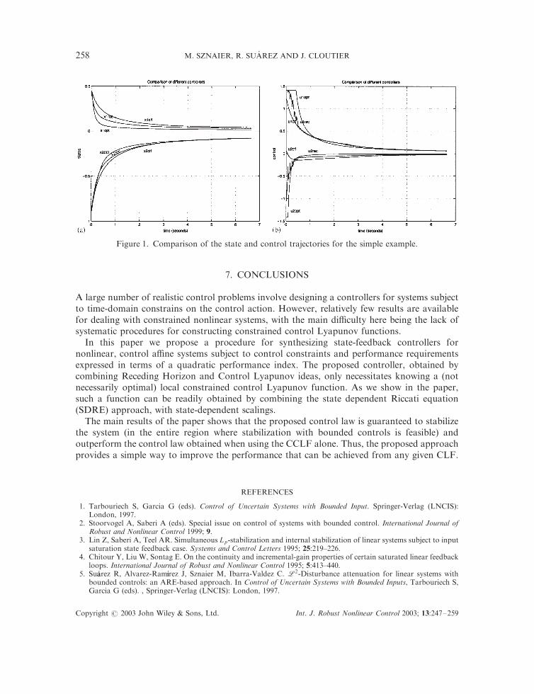
guarantees that Equations (21) and (22) hold and hence jjuðxÞjj2142 for all x 2 N:Figures 1(a) and 1(b) show a typical set of trajectories (in this case starting from the initial

condition ½0:44 � 0:88�), for the proposed controller and for the one obtained using the CCLFx0P ½x; rðxÞ�x (i.e. when setting T ¼ 0). Here we have used an horizon T ¼ 1; and assumed that thecontrol trajectory in recomputed ever T =4: For illustration purposes, we also show the optimaltrajectories obtained using off-line optimization. The corresponding costs are Jrec ¼ 0:63; JCCLF¼ 0:80; and Joptimal ¼ 0:59: Thus, even with this relatively short prediction horizon, the recedinghorizon controller achieves virtually optimal performance, yielding a 25% improvement overthe Constrained CLF based controller. Similar results were obtained for other initial conditionsand values of r:

Note that although f ðxÞ and gðxÞ in (37) are locally Lipschitz, the system cannot be linearizedat x ¼ 0: Hence approaches relying on the linearization of the system (such as the one proposedin Reference [15]) cannot be used here, even at the expense of performance.



7. CONCLUSIONS

A large number of realistic control problems involve designing a controllers for systems subjectto time-domain constrains on the control action. However, relatively few results are availablefor dealing with constrained nonlinear systems, with the main difficulty here being the lack ofsystematic procedures for constructing constrained control Lyapunov functions.

In this paper we propose a procedure for synthesizing state-feedback controllers fornonlinear, control affine systems subject to control constraints and performance requirementsexpressed in terms of a quadratic performance index. The proposed controller, obtained bycombining Receding Horizon and Control Lyapunov ideas, only necessitates knowing a (notnecessarily optimal) local constrained control Lyapunov function. As we show in the paper,such a function can be readily obtained by combining the state dependent Riccati equation(SDRE) approach, with state-dependent scalings.

The main results of the paper shows that the proposed control law is guaranteed to stabilizethe system (in the entire region where stabilization with bounded controls is feasible) andoutperform the control law obtained when using the CCLF alone. Thus, the proposed approachprovides a simple way to improve the performance that can be achieved from any given CLF.

REFERENCES

1. Tarbouriech S, Garcia G (eds). Control of Uncertain Systems with Bounded Input. Springer-Verlag (LNCIS):London, 1997.

2. Stoorvogel A, Saberi A (eds). Special issue on control of systems with bounded control. International Journal ofRobust and Nonlinear Control 1999; 9.

3. Lin Z, Saberi A, Teel AR. Simultaneous Lp-stabilization and internal stabilization of linear systems subject to inputsaturation state feedback case. Systems and Control Letters 1995; 25:219–226.

4. Chitour Y, Liu W, Sontag E. On the continuity and incremental-gain properties of certain saturated linear feedbackloops. International Journal of Robust and Nonlinear Control 1995; 5:413–440.

5. Su!aarez R, Alvarez-Ram!ıırez J, Sznaier M, Ibarra-Valdez C. L2-Disturbance attenuation for linear systems withbounded controls: an ARE-based approach. In Control of Uncertain Systems with Bounded Inputs, Tarbouriech S,Garcia G (eds). , Springer-Verlag (LNCIS): London, 1997.

Figure 1. Comparison of the state and control trajectories for the simple example.



6. Sznaier M, Suarez R, Miani S, Alvarez J. Optimal ‘1 disturbance attenuation and global stabilization of linearsystems with bounded control. International Journal of Robust and Nonlinear Control 1999; 9:659–675.

7. Krstic M, Kanellakopoulos I, Kokotovic P. Nonlinear and Adaptive Control Design. Wiley: New York, 1995.8. Artstein Z. Stabilization with relaxed control. Nonlinear Analysis 1983; 7(11):1163–1173.9. Sontag ED. A ‘universal’ construction of Artstein’s theorem on nonlinear stabilization. Systems and Control Letters

1989; 13(2):117–123.10. Sznaier M, Damborg M. Heuristically enhanced feedback control of constrained discrete time linear systems.

Automatica 1990; 26(3):521–532.11. Rossiter JA, Kouvaritakis B. Constrained generalized predictive control. Proceedings of IEE Pt. D., vol. 140. 1993;

233–254.12. Mayne DQ, Rawlings JB, Rao CV, Scokaert POM. Constrained model predictive control: stability and optimality.

Automatica 2000; 36(6):789–814.13. Mayne DQ, Michalska H. Receding horizon control of nonlinear systems. IEEE Transactions on Automatic Control

1990; 35(7):814–824.14. Primbs JA, Nevistic V, Doyle JC. On receding horizon extensions and control Lyapunov functions. Proceedings of

the 1998 American Control Conference, 1998; 3276–3280.15. Chen H, Allgower F. A quasi-infinite horizon nonlinear model predictive control scheme with guaranteed stability.

Automatica 1998; 34(10):1205–1217.16. Sznaier M, Damborg MJ. Suboptimal control of linear systems with state and control inequality constrains.

Proceedings of the 26th IEEE CDC, Los Angeles, CA, Dec. 1987; 761–762.17. Magni L, Sepulchre R. Stability margins for nonlinear receding horizon control via inverse optimality. Systems and

Control Letters 1997; 32:241–245.18. Sznaier M, Cloutier J, Hull R, Jacques D, Mracek C. A receding horizon state dependent Riccati equation approach

to suboptimal regulation of nonlinear systems. Proceedings of the 1998 IEEE CDC, 1998; 1792–1797. See also, Areceding horizon control Lyapunov function approach to suboptimal regulation of nonlinear systems. AIAA Journalof Guidance and Control 2000; 23(3):399–405.

19. Jadbabaie A, Yu J, Hauser J. Stabilizing receding horizon control of nonlinear systems: a control Lyapunovfunction approach. Proceedings of the 1999 ACC, 1999; 1535–1539.

20. Seron MM, De Dona JA, Goodwin GC. Global analytical model predictive control with input constraints.Proceedings of the 39th IEEE CDC, Dec 2000; 154–159.

21. Bemporad A, Morari M, Dua V, Pistikopoulos N. The explicit solution of model predictive control viamultiparametric quadratic programming. Proceedings of the 2000 American Control Conference, June 2000; 872–876.

22. Kouvaritakis B, Rossiter JA, Schuurmans J. Efficient robust predictive control. Proceedings of the 1999 AmericanControl Conference, 1999; 4283–4287.

23. Khalil HK. Nonlinear Systems (second edn). Prentice-Hall: Englewood Cliffs, NJ, 1996.24. Freeman RA, Kokotovic PV. Robust Nonlinear Control Design: State Space and Lyapunov Techniques. Birkhauser:

Boston, 1996.25. Mracek CP, Cloutier JR. Control design for the nonlinear benchmark problem via the state-dependent Riccati

equation method. International Journal of Robust and Nonlinear Control 1998; 8:401–433.26. Clarke FH, Ledyaev YS, Stern RJ, Wolenski PR. Nonsmooth Analysis and Control Theory. Springer: New York,

1997.



suboptimal control of constrained nonlinear systems via receding horizon constrained control...

Documents