Subjective Performance Indicators and Discretionary Bonus Pools

Madhav V. Rajan

Stefan Reichelstein

Graduate School of Business

Stanford University

November 2004 a

Abstract

This paper analyzes the effectiveness of discretionary bonus pools in utilizing subjective information for contracting purposes. We characterize the efficiency of bonus pools relative to the benchmark of optimal contracts that could have been written with objective and verifiable information. It is shown that ceteris paribus the principal prefers an increase in the number of managers participating in the bonus pool due to improved risk sharing. In a more specialized LEN setting with both verifiable and unverifiable performance indicators, we characterize the relative weights to be placed on different information signals. We also demonstrate that correlation in measurement errors has a different impact on optimal incentive schemes depending on whether the performance indicators are verifiable or merely subjective.

a We are grateful to Stan Baiman, Tim Baldenius, Jon Glover, Jack Hughes, and workshop participants at

Carnegie Mellon University, Columbia University, University of Pittsburgh, Rice University, UCLA, and Washington University for many helpful suggestions.

1

Subjective Performance Indicators and Discretionary Bonus Pools

I. INTRODUCTION “Our prior bonus plan established an annual variable bonus pool based on the company’s achievement of increased net sales and certain specified levels of “economic value added.” … In accordance with the prior bonus plan, we distributed 25% of the total bonus pool to all eligible executive officers pro rata according to their relative salary levels. The remaining 75% of the bonus pool was distributed based on each executive’s relative achievement of individual and group performance goals, as well as based on other subjective factors.” (Fresh Brands, Inc.; Proxy Statement filed with the SEC, April 12, 2002)

In many firms the provision of managerial incentives does not rely exclusively on

verifiable and objective performance indicators, such as accounting numbers, productivity

measure or the firm’s stock price. Incentives are also based on subjective measures such as

direct observations or informal reports from third parties. From a management control

perspective, it is essential to understand the constraints imposed by the non-verifiability of some

performance indicators. Much of the recent work on contracting with non-verifiable information

has focused on the dynamic interactions between a principal and a single agent.1

Our primary goal in this paper is to examine how a principal can use subjective (and

hence non-verifiable) information to create incentives for a team of agents. With multiple agents

the effectiveness of discretionary bonus pools is of particular interest. The main feature of bonus

pools in practice is that the principal commits contractually to pay out a certain amount in total

(which may vary with some underlying objective measure like overall corporate profit).

However, the exact division of the total bonus among the participating agents is not specified in

the contract.2

1 For instance, the papers by Bull (1987), Baker el al. (1994), Pearce and Stacchetti (1998) and Levin (2003) fall into this camp. 2 For a recent example, consider the following excerpt from Micron Technology’s proxy statement, filed with the SEC on October 18, 2002: “Cash bonuses to executive officers are intended to reward executive officers for the Company's financial performance during each fiscal year. Accordingly, bonuses are determined based on performance criteria established at the beginning of each fiscal year formulated primarily as a percentage of the Company's profits at the end of the fiscal year. Performance bonus percentages are established according to a

2

For the purposes of our model we interpret a bonus pool as an “implicit” contracting

arrangement in which a principal (e.g., the compensation committee or a departmental manager)

communicates to a group of agents how she will divide a total amount of money depending on

the realization of certain information variables. The agents choose their productive contribution

anticipating that the principal will indeed allocate the pool as promised since ex-post she has no

incentive to do otherwise.3 In comparison to a benchmark setting in which the information

variables available to the principal are verifiable for contracting purposes, the key restriction of

bonus pools is that the total payout must remain invariant to the observed outcomes.

Our first question is whether one can find incentive schemes that perform better than

bonus pools if the principal can rely only on subjective performance indicators. In a one-agent

model, MacLeod (2003) has shown that it may be optimal to involve “third parties.” Under

these schemes, the principal retains discretion as to whether a given amount of money is paid out

entirely to the agent or partly diverted to a third party (such as a charitable organization)

depending on the realization of some subjective signals.4 We demonstrate that with subjective

information only and two or more agents it is optimal for the principal to set up a discretionary

bonus pool. Thus, there is no need to divert compensation to third parties.5

Bonus pools entail an additional agency cost relative to the hypothetical second-best

benchmark in which the principal’s information is verifiable and contractible. Agents must be

burdened with additional risk due to the balancing requirement inherent in bonus pools. The

resulting performance level may be viewed as third-best and our analysis seeks to capture the

subjective analysis of each executive officer's contribution to the Company according to the same criteria utilized to determine base salary.” 3 In our one-period model, the principal is indifferent about carrying out the terms of the implicit contract. This indifference will be supplanted by reputation concerns in a multi-period model. It would be desirable for future research on implicit contracts to capture the interactions between multiple agents and multiple time periods. 4 Given the monotone likelihood ratio property, MacLeod (2003) demonstrates that the optimal third party scheme is to pay the agent the entire amount unless the principal observes the lowest possible outcome. 5 If the agents observe signals that are correlated with the subjective signals received by the principal, then it may benefit the principal to set up “message sending” games in which the agents’ payoffs are determined according to messages sent by the parties; see MacLeod (2003). We discuss the class of admissible mechanisms in more detail in Section II below.

3

attendant cost to the principal. The primary motivation for studying this cost is to understand the

constraints imposed by subjective information. At the same time our results shed light on the

agency costs associated with implicit rather than explicit contracts. An alternative motivation

for our study is that all information variables are fully contractible yet because of the costs of

writing and enforcing multi-agent incentive contracts, the principal may opt for a “simpler”

bonus pool arrangement. Such arrangements are contractually incomplete beyond the principal’s

commitment for a fixed collective payout. While it has been difficult for the theory of contracts

to capture the costs of contracting, our results do speak to the relative loss associated with

implicit contracts, i.e., bonus pools.6

To understand the relative agency costs associated with subjective performance

indicators, we consider several specialized settings. When the signals available to the principal

reflect the agents’ efforts perfectly, the first-best can, of course, be attained with verifiable

signals. We find that with perfect observability bonus pools also achieve the first-best.

Depending on the feasibility of sufficiently large punishments, the first-best can in fact be

attained in dominant strategies. In the presence of limited liability constraints, the first-best will

still be attainable as the unique strategy that emerges when agents sequentially eliminate any

strictly dominated strategies.

One would expect that ceteris paribus the balancing requirement associated with bonus

pools would be less severe for a larger group of agents. We demonstrate this effect for the case

of -identical agents and stochastically independent signals. Intuitively, the balancing

requirement of a bonus pool implies that the variance associated with agent i ’s incentive scheme

be spread among the remaining agents. As in a portfolio with independent securities, the

effective risk imposed on each of the other

n

1−n

1−n agents is then to the order of 21

1n⎛ ⎞⎜ ⎟−⎝ ⎠

of the

variance of agents i ’s incentive compensation. Formally, we demonstrate that the loss

associated with bonus pools, relative to the second-best benchmark, declines on a per-capita 6 Earlier literature has formalized alternative notions of costly contracting to explain delegation and delegated contracting. See Dye (1985), Melumad et al. (1997) and Laffont and Martimort (2001) on this point.

4

basis for an increasing number of agents. In interpreting this result, it should be noted that we

are holding the quality of the subjective information signals fixed for each agent as the size of

the team increases. Thus our model abstracts from any confounding “span of control” effects.

A familiar result in the agency literature is that when multiple signals are informative

about an agent’s action, the signals should be aggregated according to their signal-to-noise ratios

for contracting purposes.7 We revisit this finding for a setting in which the principal obtains an

objective (verifiable) and a subjective (unverifiable) signal for each agent. In the context of the

so-called LEN model, we find that the weight placed on the subjective signal relative to that on

the objective signal is less than the signal-to-noise ratio of these two variables. This distortion

again reflects the balancing requirement associated with bonus pools. In the case of -identical

agents, the optimal ratio between the two signals is equal to

n( 1)n

n− times the signal-to-noise ratio.

Thus the subjectivity of a signal reduces its optimal weight by a factor of one half when there are

two agents, yet the distortion caused by subjectivity diminishes quickly for larger values of . n

Our final point investigates the performance of bonus pools under the assumption that the

measurement errors are correlated across agents. For the benchmark setting of verifiable signals,

the principal can exploit any correlation by employing a suitable relative performance evaluation

scheme. Specifically, in the two-agent LEN model, the principal’s cost turns out to be a

quadratic function of the correlation coefficient between the random disturbances affecting the

agents’ signals, with the maximum cost occurring at zero (i.e., no correlation). In contrast, with

subjective performance indicators the principal only benefits from positive correlation. Since

any relative performance evaluation scheme is again subject to the requirement of a bonus pool,

the principal’s cost is monotonically decreasing in the amount of correlation, with perfect

negative correlation representing the least useful subjective information.

Regarding prior work on incentive contracting with subjective information, our work is

most closely related to MacLeod (2003) and Baiman and Rajan (1995). The latter authors

7 Banker and Datar (1989) have established this result for a class of probability distributions that includes the exponential family.

5

examine a two-agent setting and find that there is positive value to using a bonus pool that

utilizes an unverifiable signal about one of the managers. Our results extend their work along

several dimensions by identifying environments in which discretionary bonus pools are optimal,

measuring the additional agency costs imposed by subjective information and by characterizing

the optimal weights to be placed on subjective as opposed to objective signals.8

The remainder of the paper is organized as follows. The next section examines the

effectiveness of bonus pools when the principal has access only to subjective measures. Section

III considers the interplay of subjective and objective indicators in the context of a LEN model.

Conclusions and directions for future work are presented in Section IV.

II. SUBJECTIVE PERFORMANCE INDICATORS

We study a multi-agent moral hazard problem in which the principal’s information about

the agents’ productive contributions is subjective. This information cannot be verified to

external parties, and therefore it is impossible to condition formal incentive contracts on this

information. Our analysis focuses on a fixed effort level, , that the owner wishes to induce

from each agent.

0ia

9 Conditional on each agent’s unobservable action choice, the principal

observes a subjective signal, , which is informative about the action taken by agent i .iy 10

8 In addition to the analytical work discussed above, there is some relevant empirical evidence on subjective performance measures and bonus schemes. Brown (1990) considers the determinants of standard rate pay, subjective merit pay, and piece rates for a large sample of workers and finds that the likelihood of piece rate pay is decreasing in the diversity of duties carried out by an agent. Similarly, MacLeod and Parent (1998) show that jobs involving many tasks are typically characterized by subjective assessments of performance. Hayes and Schaefer (2000) report evidence consistent with the use of subjective assessments when boards of directors decide the salary and bonus of chief executives. Gibbs et al. (2004) find that discretionary bonuses are used to balance perceived flaws in quantitative performance measures and insure employees against downside risk in their compensation. Finally, the experimental literature has also studied the use of opportunism in the presence of subjective measures. Fisher et al. (2003) test, and find support for, the theoretical results in Baiman and Rajan (1995) regarding the usefulness of objective bonus pools with discretionary ex post distributions. 9 In other words, we follow the cost minimization approach first employed by Grossman and Hart (1983). 10 The signal may or may not be observed by agent i. We discuss this aspect in more detail below. For the purposes of our analysis we presume that all subjective information is non-verifiable (and all objective information is verifiable), even though multiple parties may have access to the subjective information.

iy

6

Given the absence of objective, contractible information, one possible mechanism for the

principal is to use a third-party scheme, as proposed by MacLeod (2003) in the context of a

single agent. Under such a scheme, the principal commits to paying out the same amount

irrespective of his information. However, the amount paid to the agent depends on the

subjective information received by the principal. For certain contingencies, for instance if the

subjective information is indicative of shirking on the part of the manager, the principal can

choose to redirect some or all of the amount to an outside third-party, such as a charity. Since

the owner is ex-post indifferent as to the recipient of this fixed outlay, the presumption is that he

will employ the course of action that is most efficient from an ex-ante standpoint. The

principal’s implicit contract with the agent therefore specifies how a fixed amount of money will

be divided between the agent and the third party depending on the observed signal.

The main question we address is how the presence of multiple agents alters the nature of

the principal’s compensation design when the performance indicators about all agents remain

subjective. One feasible alternative is to replicate the third-party scheme for each manager. The

advantage of this approach would be that each agent’s payoff is based only on the signal that is

informative about his own effort. Alternatively, the presence of a second manager raises the

possibility that the principal can pay compensation to that manager rather than “waste” money

by giving it to charity. As a consequence, however, each agent will be subjected to extraneous

random fluctuations associated with the other agent’s signal.

For notational convenience, we first consider a two-agent setting with simultaneous

action choices. The subjective signals available to the principal have their support on the

finite sets {yiy

i1, yi2, …, yiMi}, respectively. Manager 1’s action, 11 1 ,a a a ,⎡ ⎤∈ ⎣ ⎦ induces density

1 1f(y |a ) while manager 2’s action, 22 2 ,a a a ,⎡ ⎤∈ ⎣ ⎦ induces density g(y2|a2) on the respective

sets of possible signal realizations. Throughout this section, the information signals are assumed

to be independent of each other. Agents are assumed to be risk-averse with preferences that are

additively separable over wealth, ( )iU ⋅ , and the cost of effort, ( )ie ⋅ .

7

Program P1: Minw, cjk, sjk

w

subject to: ( )0 0 0

1 1 2 1 1( ) | , ( )jkE U c a a e a U− ≥ 1 (1)

( )0 0 02 1 2 2 2( ) | , ( )jkE U s a a e a U− ≥ 2

1 1⎤− ⎦

2 2⎤− ⎦

w

(2)

( )1

0 01 1 1 2max ( ) | , ( )a jka arg E U c a a e a⎡∈ ⎣ (3)

( )2

0 02 2 1 2max ( ) | , ( )a jka arg E U s a a e a⎡∈ ⎣ (4)

For all {j,k}, (5) 0.jk jkw c s− − ≥

The variables cjk and sjk represent the compensation payments that the principal

“promises” to managers 1 and 2, respectively, when the signal realizations are {y1j, y2k}. We

refer to the third-party schemes in P1 as fixed payment schemes. A fixed payment scheme is said to be a discretionary bonus pool arrangement if (5) holds as an equality, i.e., for all

j, k. In other words, with n agents, a fixed payment scheme is a discretionary bonus pool

arrangement if and only if participant (n+1), the outsider, receives zero compensation in every

contingency.

jk jkc s+ =

It is important at this stage to be explicit about the class of admissible incentive

mechanisms. With non-verifiable information, the parties can conceivably enter into a contract

specifying payments as a function of messages that the principal and the agent send after

receiving subjective information. In a single agent setting, MacLeod (2003) shows that if both

parties observe the non-verifiable signal y, then it is possible to construct a message game and a

corresponding outcome function (that involves the use of a third party) so as to achieve second-

best performance in equilibrium (Proposition 4 in MacLeod, 2003).11 On the other hand, if only

the principal observes y, then message games cannot sustain any outcome beyond those

attainable by third-party schemes. This follows immediately from the fact that, by the

11 It should be noted, however, that such mechanisms are necessarily afflicted by multiple equilibrium problems. Any pair of messages that forms an equilibrium in one state (agent’s action and signal realization) also forms an equilibrium in any other state.

8

Revelation Principle, equilibrium messages must amount to truthful reporting. Yet, if the

principal is to report her observation truthfully, her payoff must be the same for all realizations

of the signal.

In ruling out mechanisms based on messages sent by the parties, we may either follow

MacLeod’s argument and suppose that the subjective signals observed by the principal are not

available to the agents; for instance, the principal may rely on direct observations or collect

informal reports from various sources. Alternatively, the subjective nature of the performance

indicators may make it too costly to write a contract based on the parties’ reports about their

observations. This alternative justification appeals to the notion that the principal can effectively

communicate incentive provisions tied to the subjective performance indicators, yet it would be

too costly to specify this rule as part of an explicit, legally binding contract.

To characterize the solution to Program P1, we assume that the first-order approach is

valid. Earlier literature has specified a variety of sufficient conditions ensuring the validity of

this approach (e.g., Jewitt 1988, Sinclair-Desgagne 1994).12

Assumption (A1): The first-order approach is valid, i.e., the incentive constraints for managers

1 and 2 can be equivalently represented as follows:

(6) 1 2

0 0 01 1 1 2 2 1 1

1 1

( ) ( | ) ( | ) ( ) 0M M

jk a j kj k

U c f y a g y a e a= =

′−∑∑ =

=

(7) 1 2

0 0 02 1 1 2 2 2 2

1 1

( ) ( | ) ( | ) ( ) 0M M

jk j a kj k

U s f y a g y a e a= =

′−∑∑

Proposition 1: Suppose (A1) holds. With subjective performance indicators, a discretionary

bonus pool arrangement is optimal among all fixed payment schemes.

12 The validity of the first-order approach is only an issue in Proposition 1. One sufficient condition for the validity of this approach in the context of our model is that the agent’s action determines a convex combination of two given densities; see MacLeod (2003) for details.

9

In contrast to MacLeod’s (2003) finding about the need for involving third-parties, we

conclude that it is always efficient for the principal to pay out the entire amount to the two agents

collectively, irrespective of the actual signal realizations. To provide efficient incentives for

each agent, the principal wants to use the other agent as a budget-balancer.

It is instructive to ask how the compensation payments vary with the observed signals.

Provided the familiar Monotone Likelihood Ratio Property (MLRP) holds, it can be shown that

each manager’s compensation is an increasing function of his own signal realization and a

decreasing function of the other manager’s signal realization. Therefore each manager benefits

from poor performance by the other manager, highlighting the need for relative performance

evaluation when information is subjective. As a further consequence of the MLRP property, it

can be shown that for an optimal bonus pool arrangement “shirking” will not be an equilibrium

strategy for both agents. In particular, it can be shown that a manager who conjectures that the

other manager plans to take the lowest possible action will not reciprocate since he can capture a

larger share of the pool by increasing his own subjective metric.

While Proposition 1 has shown that there is no need for third-party schemes with at least

two agents, the subjectivity of the principal’s information is nonetheless costly.

Proposition 2: Discretionary bonus pools entail an additional cost for the principal relative to

the benchmark setting of objective (contractible) performance indicators.

In the benchmark setting, each manager receives an incentive scheme that depends only on

the signal realizations that are informative about his own actions. The bonus pool results in a

loss of efficiency relative to the benchmark setting precisely because the balancing requirement

inherent in bonus pools. Put differently, any bonus pool could be improved upon if the

information variables were to be contractible. iy

10

The remainder of this section characterizes the incremental cost associated with

subjective information. Specifically, we focus on environments in which this cost is small. To

that end, suppose first that the performance indicators are perfect in the sense that there is a

continuum of signal outcomes, , such that iy iy ai= . Obviously, the first-best can be achieved in

the benchmark setting of verifiable information. The following result shows that the same

performance is attainable if the perfect information is merely subjective.

Proposition 3: With perfect subjective information, discretionary bonus pools can implement

first-best performance in dominant strategies.

One might expect difficulties in achieving first-best outcomes in dominant strategies.

Due to the balancing requirement inherent in bonus pools, it is impossible to punish both

managers for not taking the target action. The construction in the proof of Proposition 3 pays

each agent the same regardless of whether both agents are “obedient” (i.e., choose ) or “shirk”

(i.e., do not choose ). Still, dominant strategy incentives obtain provided (i) an agent receives

a large reward for being obedient when the other agent shirks and (ii) an agent receives a large

penalty for shirking whenever the other agent was obedient.

0ia

0ia

The construction in Proposition 3 relies on the feasibility of inflicting large penalties for

shirking (see the proof of Proposition 3 for details). It is therefore important to ask whether first-

best performance is still attainable if compensation is restricted to be non-negative, i.e.,

and . The following result shows that the first-best remains attainable despite this limited

liability constraint, provided the solution concept is weakened somewhat.

1 0c ≥

2 0s ≥

Corollary 1: Suppose compensation payments are restricted to be non-negative. With perfect

subjective information, first-best performance can be implemented as the unique outcome

surviving iterated elimination of strictly dominated strategies.

11

The proof of Corollary 1 is similar to that of Proposition 3, except that now only agent 1

has a dominant strategy. In particular, that agent will receive a payment of zero for shirking,

independently of the other agent’s action. Given agent 1’s dominant strategy for obedience, it

then becomes a best response for agent 2 to be obedient as well.

To check the robustness of our findings in Proposition 3 and its corollary, suppose the

principal were to observe subjective information that was “close to perfect” in accuracy. Since

our implementation is based on strict dominance solvability, our findings still obtain. For the

corollary, in particular, suppose that the subjective information is slightly noisy in that the Type I

and Type II errors, Prob{Principal observes “Not ”|Manager chooses } and Prob{Principal

observes |Manager chooses “Not ”} are less than some

0ia 0

ia0ia 0

ia > 0ε . For ε below ε , it is easy to

see that the mechanism in the proof of Corollary 1 still implements the desired actions, though

the principal now has to pay an additional risk premium which increases monotonically in ε .

For further insight into the relative costs associated with subjective information and

implicit contracts, we now turn to an n-agent setting. Intuitively, the additional costs associated

with bonus pools should diminish for a larger number of participants in the pool. If the variation

in any agent’s compensation can be divided among a larger number of participants, the per capita

risk premium should become smaller.13 To study the performance of bonus pools with an

increasing number of agents, we will confine attention to a setting with identical agents. To

examine that intuition formally, we first note that the above results extend without change to

more than two agents.14

Corollary 2: Propositions 1-3 and Corollary 1 extend to an arbitrary number of agents, n, with

n ≥ 2.

13 This intuition is consistent with the survey finding in Fox (1979) that the median number of participants in bonus pools was a relatively high 139. 14 In the Appendix, we construct a mechanism under which the desired actions are dominant strategies for all but one agent. Conditional on these choices, the desired action is then a best response for the remaining agent.

12

Suppose now there are n-identical agents. For the benchmark setting of verifiable

information, let denote the principal’s expected cost of inducing any one agent to

implement the action . As observed above, with verifiable information and n agents the

principal’s cost then becomes . By comparison, let denote the principal’s cost under

the optimal contract with subjective information. Proposition 2 has shown that >

for any n. The first question to be addressed is whether the per capita cost of bonus pools,

, is monotonically decreasing in n. We establish this monotonicity for a setting with

binary signals for each agent. Without loss of generality, each agent’s action can then be

identified with the probability of achieving a “success.”

*C

0a

*n C⋅ ( )C n

( ) /C n n *C

( ) /C n n

Proposition 4: With n identical agents, the per-capita size of the optimal bonus pool is strictly

decreasing in n, that is:

( )C nn

> ( )1.

1C n

n++

The complex, constructive proof of this result essentially uses the optimal bonus pool

from the n-agent case to design an artificial bonus pool for the (n+1)-agent case that provides

more efficient incentives overall. Specifically, the new set of compensation payments are

constructed to share the same support as in the n-manager setting and provide the same level of

expected compensation. However, outcome by outcome, the payments for the larger pool entail

less risk for each agent, which in turn allows the size of the average pool to be reduced.

The natural question at this stage is whether the per-capita cost of bonus pools approaches

the benchmark cost C* as the number of agents gets large. As this result only pertains to the

limit, it is computationally no longer of importance to have only binary signals. At the same

time, it will be convenient to ignore small wealth effects so as to assure that a particular action

profile is indeed an equilibrium, in fact, a dominant strategy equilibrium. Accordingly, we

assume constant absolute risk aversion for all agents.

13

Assumption (A2): Agents have CARA utility of the form: ( ) ( )( ){ }ˆ, expi i i i i i iU s a k s e a= − − ⋅ − .

Proposition 5: Given (A2) and n-identical agents, ( ) *C n

Cn

→ as n → ∞.

With a large number of managers, bonus pool mechanisms are thus as cost-efficient as

explicit contracts based on verifiable information. The introduction of additional independent

draws, (i.e., the outcomes of additional managers) gradually eliminates the risk imposed on each

manager as a result of the budget balancing requirement. The bonus pool mechanism we use in

the proof of Proposition 5 seeks to compensate each manager according to the optimal contract

with verifiable information; any difference between the manager’s pay and the ex ante expected

level of pay under the second-best contract is then distributed equally among the other ( 1)n −

managers. For large n, the weak law of large numbers ensures that the extraneous risk on each

manager can be reduced to arbitrarily low levels.15

In interpreting the above result, it is important to keep in mind that the principal’s ability

to receive and process subjective performance indicators is assumed to be unaffected by an

increase in the number of agents. Outside our model, one would expect “span of control”

limitations related to communication and information processing to be a factor that constrains

the number of participants in a bonus pool. While our analysis does not explicitly incorporate

any such cost factors, it does speak to the potential benefit of adding more agents. To that end,

the following section considers a more specialized contracting model in which we can track the

speed of convergence at which the per-capita cost of bonus pools approaches the benchmark

level.

15 As noted above, our use of CARA utility for this result is primarily for technical convenience. Alternatively, we can show that for any utility function, the bonus pool construction employed in the proof of Proposition 5 implements an action vector arbitrarily close to the desired one, at a cost that approximates second-best, for large values of n.

14

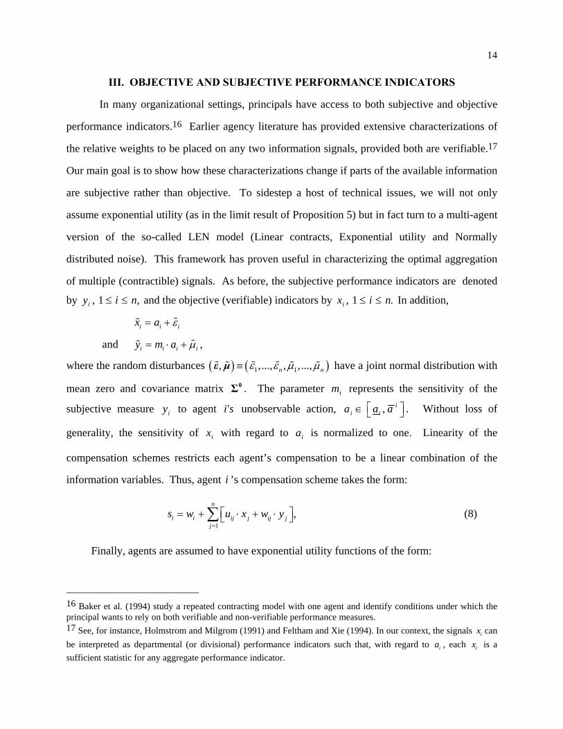
III. OBJECTIVE AND SUBJECTIVE PERFORMANCE INDICATORS

In many organizational settings, principals have access to both subjective and objective

performance indicators.16 Earlier agency literature has provided extensive characterizations of

the relative weights to be placed on any two information signals, provided both are verifiable.17

Our main goal is to show how these characterizations change if parts of the available information

are subjective rather than objective. To sidestep a host of technical issues, we will not only

assume exponential utility (as in the limit result of Proposition 5) but in fact turn to a multi-agent

version of the so-called LEN model (Linear contracts, Exponential utility and Normally

distributed noise). This framework has proven useful in characterizing the optimal aggregation

of multiple (contractible) signals. As before, the subjective performance indicators are denoted

by , 1 and the objective (verifiable) indicators by , 1iy ,i n≤ ≤ ix .i n≤ ≤ In addition,

i ix a iε= + %%

and i i iy m a iµ= ⋅ + %% ,

where the random disturbances ( ) ( )1 1, ,..., , ,...,n nε ε µ µ≡% % %% %ε µ % have a joint normal distribution with

mean zero and covariance matrix . The parameter represents the sensitivity of the

subjective measure to agent unobservable action,

0Σ im

iy si ' , ii ia a a .⎡ ⎤∈ ⎣ ⎦ Without loss of

generality, the sensitivity of with regard to is normalized to one. Linearity of the

compensation schemes restricts each agent’s compensation to be a linear combination of the

information variables. Thus, agent i ’s compensation scheme takes the form:

ix ia

(8) 1

,n

i i ij j ij jj

s w u x w y=

⎡= + ⋅ + ⋅⎣∑ ⎤⎦

Finally, agents are assumed to have exponential utility functions of the form:

16 Baker et al. (1994) study a repeated contracting model with one agent and identify conditions under which the principal wants to rely on both verifiable and non-verifiable performance measures. 17 See, for instance, Holmstrom and Milgrom (1991) and Feltham and Xie (1994). In our context, the signals ix can be interpreted as departmental (or divisional) performance indicators such that, with regard to , each ia ix is a sufficient statistic for any aggregate performance indicator.

15

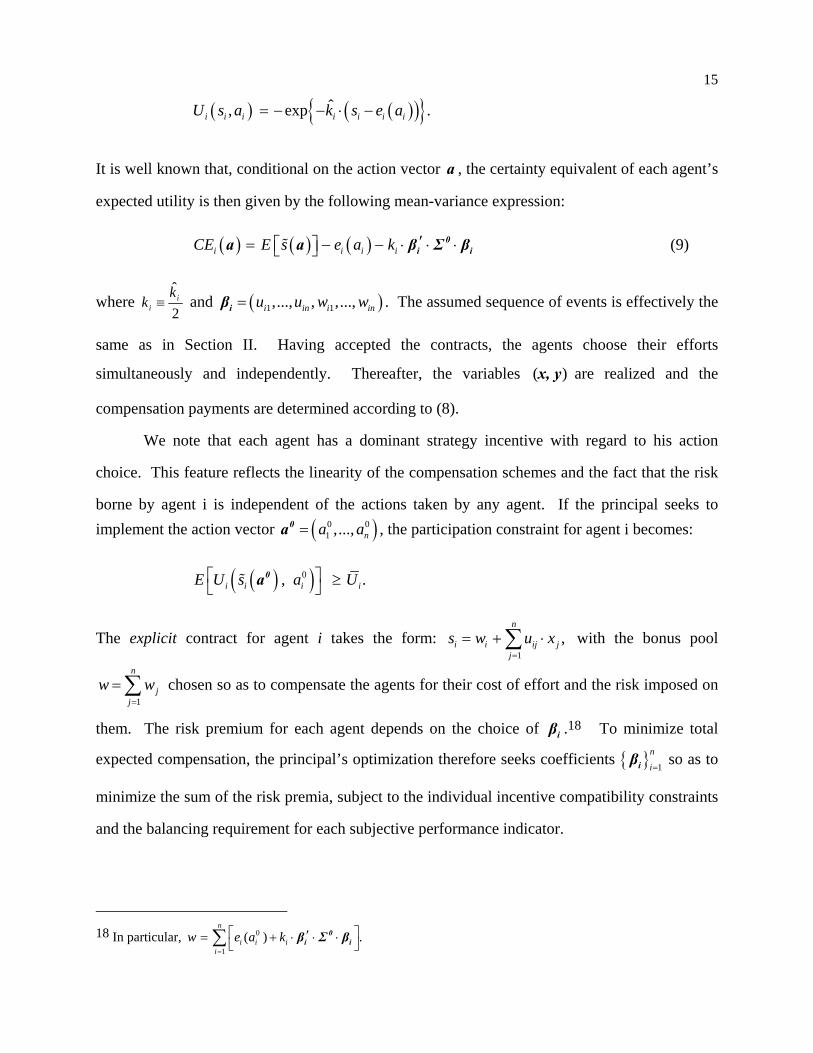
( ) ( )( ){ }ˆ, expi i i i i i iU s a k s e a= − − ⋅ − .

⋅ i

It is well known that, conditional on the action vector a , the certainty equivalent of each agent’s

expected utility is then given by the following mean-variance expression:

( ) ( ) ( )i i i iCE E s e a k ′= − − ⋅ ⋅⎡ ⎤⎣ ⎦% 0ia a β Σ β (9)

where 2

ˆi

i

kk ≡ and . The assumed sequence of events is effectively the

same as in Section II. Having accepted the contracts, the agents choose their efforts

simultaneously and independently. Thereafter, the variables

( 1 1,..., , ,...,i in i iu u w w=iβ )n

( ) x, y are realized and the

compensation payments are determined according to (8).

We note that each agent has a dominant strategy incentive with regard to his action

choice. This feature reflects the linearity of the compensation schemes and the fact that the risk

borne by agent i is independent of the actions taken by any agent. If the principal seeks to implement the action vector , the participation constraint for agent i becomes: ( 0

1 ,..., na a=0a )0

( )( )0, .i i i iE U s a U⎡ ⎤ ≥⎣ ⎦% 0a

The explicit contract for agent i takes the form: 1

,n

i i ij jj

s w u x=

= + ⋅∑ with the bonus pool

chosen so as to compensate the agents for their cost of effort and the risk imposed on

them. The risk premium for each agent depends on the choice of

1

n

jj

w w=

= ∑

iβ .18 To minimize total

expected compensation, the principal’s optimization therefore seeks coefficients { } so as to

minimize the sum of the risk premia, subject to the individual incentive compatibility constraints

and the balancing requirement for each subjective performance indicator.

1

n

i=iβ

.⋅18 In particular, 0

1

( )n

i i ii

w e a k=

⎡ ⎤′= + ⋅ ⋅⎣ ⎦∑ 0

i iβ Σ β

16

Program P2: { }1

n

ii

Min k=

′⋅ ⋅ ⋅∑i

0i iβ β Σ β

subject to: for( )0 ,i ii ii i im w u e a′⋅ + = 1 ,i n≤ ≤

for1

0,n

iji

w=

=∑ 1 .j n≤ ≤

In the current linear framework, the balancing requirement inherent in a bonus pool requires that

any choice of bonus coefficient must be absorbed collectively by the other n-1 agents. Thus,

the principal faces a quadratic cost minimization problem in the variables {iiw

},ij iju w , subject to 2n

linear constraints.

3.1 Independent Signals

To begin with, the random disturbances are assumed to be mutually independent. As a

consequence, it is only the balancing condition of the bonus pool that connects agents in the

optimization problem P2.

Assumption (A3): The random variables ( )% %ε, µ are mutually independent with

( ) 2iVar iε σ=% and ( ) 2.i iVar µ η=%

With stochastic independence among all information variables, there is clearly no need for relative performance evaluation with regard to the verifiable signals, i.e., for 0iju = i j≠ . If

the realization of were hypothetically verifiable, agent i’s compensation would

depend only on x

( 1,.., ny y )

i and yi. Furthermore, the relative weights placed on these two variables would

be given by their signal-to-noise ratio, i.e., the ratio of their sensitivities relative to their

precisions. In our model, this ratio reduces to:

2

2 ,oii i

ioii i

w mu

ση

= ⋅ (10)

17

since the ratio of sensitivity to precision for is given by iy 2i

i

mη

. Intuitively, one would expect the

non-verifiability of to increase the agency cost associated with these variables.

Higher values of motivate agent i to exert more effort, yet the principal must pay a

corresponding risk premium not only to agent i but also to agent j in order to maintain a bonus

pool. Since the marginal risk premium of the signal y

( 1,.., ny y )

iw

i is zero at 0iiw = (due to the quadratic

objective function in P2), it is immediate that, despite the constraints imposed by subjectivity, an

optimal contract never puts zero weight on any yi. At the same time, subjectivity entails a

distortion which will be reflected in the choice of optimal coefficients and iiu∗iiw∗ . The

magnitude of this distortion is readily identified in a setting with -identical agents where

n

,ik k= 0 0 ,ia a= ,im m= 2 2 ,iσ σ= 2 and 2iη η= for all 1 .i n≤ ≤

Proposition 6: Given the stochastic independence condition (A3),

i) the optimal coefficients in P2 are such that, for each agent, the ratio of the optimal

weights on yi and xi is positive but less than the signal-to-noise ratio of yi and xi.

ii) With n -identical agents, this ratio is given by:

2

2

1 .ii

ii

w n mu n

ση

∗

∗

⎡ ⎤−= ⋅ ⋅⎢ ⎥

⎣ ⎦

Proposition 6 formalizes the intuition that because the restriction to bonus pools entails an

externality in risk bearing, subjective performance indicators receive less weight in optimal

contracts than objective, contractible indicators. With n-identical agents the principal seeks to

spread the bonus pool risk associated with the subjective variables, yi, equally among the other (n-1) agents. As the number of agents gets larger, the fact that the variables ( ) are

subjective becomes less significant and the resulting performance measures approach the ones

corresponding to the traditional signal-to-noise ratio. The distortion in the relative weighting of

1, , ny yK

18

the two signals is largest for the case of two agents. The weight put on the subjective indicator is

then just one half of what would it could have been if yi had been verifiable.

Proposition 5 in Section II has shown that if the principal has access only to unverifiable

signals, the incremental agency cost associated with bonus pools diminishes on a per capita basis

as the number of agents participating in the bonus pool increases. This result can also be

obtained when there is both objective and subjective information. In addition, we can now show

that in the LEN framework the per capita bonus pool converges to the benchmark performance at

the rate of 1 .n

Put differently, the difference between the per capita cost of a bonus pool and the

benchmark cost has order of 1 .n

19

Corollary to Proposition 6: Given (A3) and n-identical agents,

i) ( )C nn

> ( )1;

1C n

n++

ii) ( ) 1*C n

C On n

⎛ ⎞− ∈ ⎜ ⎟⎝ ⎠

.

To understand intuitively why the per-capita cost approaches the benchmark level at the

rate of 1n

, we note that the incremental risk premium required by each agent is to the order of 21

1n⎛ ⎞⎜ ⎟−⎝ ⎠

for each of the subjective signals. As mentioned in Section III, our finding that bonus

pools tend to become more efficient with an increasing number of participants ignores any costs

related to a limited “span of control” for the principal. Future work may be able to integrate the

19 The function is said to have order ( )f n 1

n, denoted as 1( )f n O

n⎛ ⎞∈ ⎜ ⎟⎝ ⎠

, if for some constant, K, and 0 ,n n≥

( ) Kf nn

≤ .

19

explicit formula derived for in the LEN framework into a model that captures the notion

that the quality of the principal’s information decays as the number of agents increases.

( )C n

20

3.2 Correlated Signals

In many situations of interest, the measurement errors will be correlated across agents.

Specifically, we examine how correlation among the subjective measures affects the bonus pool

requirement associated with unverifiable information. To minimize notational complexities, we

will focus in the subsequent analysis on the case of two agents who are identical in terms of their

productivity and preferences.

Consider first a hypothetical scenario in which the subjective measures are useless

(possibly because 2η is “large”). If the objective measures were perfectly correlated, the

principal clearly would not incur any agency cost. Though uninformative about , the variable

is fully informative about

1a

2x 1ε% (for any conjectured level of ) and therefore the noise

associated with

2a

1ε% can be eliminated entirely by setting .ii iju u= − Conversely, the principal

would incur no agency cost for perfect negative correlation since in that case eliminates

all random fluctuations. For any level of imperfect correlation between two verifiable signals,

there would be some agency costs, but this cost could be lowered by a relative performance

evaluation scheme. Simple calculations show that the principal’s cost is quadratic and it does

not matter whether the correlation is positive or negative. This cost is illustrated by the solid

curve in Figure 1.

ii iju u=

21

20 Such organizational diseconomies of scale are examined in Huddart and Liang (2003, 2004). In a multi-agent LEN framework, they analyze the optimal size of partnerships. Since partnerships must disburse all proceeds among the partners (agents), the organization faces balancing constraints akin to the ones caused by subjectivity in our model. Huddart and Liang show that diminishing returns to monitoring make it ultimately inefficient to add more partners. Our analysis here is closer in spirit to that of Holmstrom (1982) demonstrating, in the context of objective and contractible information signals, that larger teams can achieve more efficient risk sharing, holding effort incentives constant. 21 Baldenius et al. (2002) analyze a two-agent setting with verifiable and correlated signals to compare alternative monitoring structures.

20

It is also instructive to consider a second hypothetical scenario in which the verifiable

signals are useless (possibly due to large values of 2σ ) and the two subjective signals are

correlated. We note that with perfect positive correlation between and , the restriction to

bonus pools imposes no cost on the principal. For the purpose of relative performance evaluation, the principal seeks to set

1y 2y

ii ijw w= − so as to eliminate the entire noise and this choice

conforms precisely to a bonus pool. In sharp contrast, the bonus pool requirement collides head-

on with the notion of relative performance evaluation when the two signals are negatively

correlated. This observation suggests that unlike the case of unverifiable signals, the principal is

worse off by any negative correlation among the subjective performance indicators.

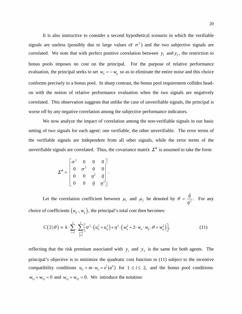
We now analyze the impact of correlation among the non-verifiable signals in our basic

setting of two signals for each agent: one verifiable, the other unverifiable. The error terms of

the verifiable signals are independent from all other signals, while the error terms of the

unverifiable signals are correlated. Thus, the covariance matrix 0Σ is assumed to take the form:

2

2

2

2

0 0 00 0

ˆ0 0ˆ0 0

σσ 0

η ηη η

⎡ ⎤⎢ ⎥⎢ ⎥=⎢ ⎥⎢ ⎥⎣ ⎦

0Σ .

Let the correlation coefficient between 1µ and 2µ be denoted by 2

ηθη

= . For any

choice of coefficients ( , the principal’s total cost then becomes: ),ij iju w

( ) ( ) ( )2 2

2 2 2 2 2 2

1 1

2 | 2 ,ii ij ii ii ij iji j

j i

C k u u w w w wθ σ η θ= =

≠

⎡ ⎤≡ ⋅ ⋅ + + ⋅ + ⋅ ⋅ ⋅ +⎣ ⎦∑ ∑ (11)

reflecting that the risk premium associated with and is the same for both agents. The

principal’s objective is to minimize the quadratic cost function in (11) subject to the incentive

compatibility conditions for 1

1y 2y

0( )ii iiu m w e a′+ ⋅ = 2,i≤ ≤ and the bonus pool conditions:

and We introduce the notation: 11 21 0w w+ = 12 22 0.w w+ =

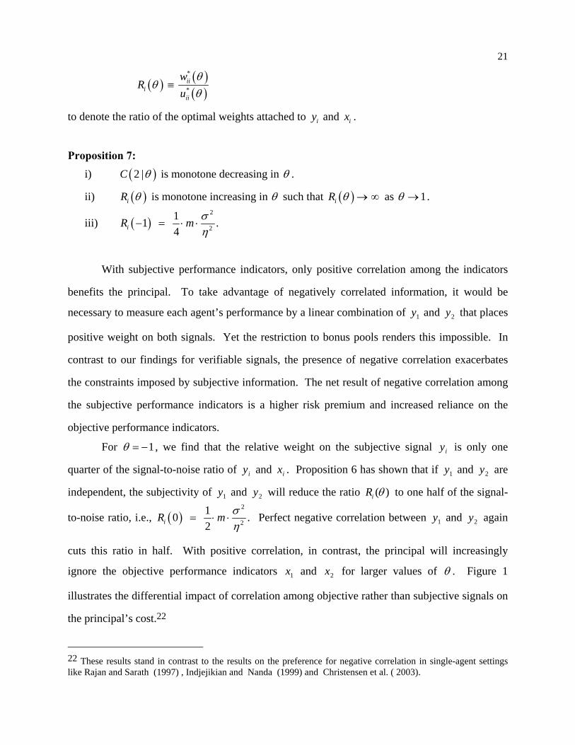
21

( ) ( )( )

*

*ii

iii

wR

uθ

θθ

≡

to denote the ratio of the optimal weights attached to and iy ix .

Proposition 7: i) (2 |C )θ is monotone decreasing in θ .

ii) ( )iR θ is monotone increasing in θ such that ( )iR θ → ∞ as 1θ → .

iii) ( )2

2

11 .4iR m σ

η− = ⋅ ⋅

With subjective performance indicators, only positive correlation among the indicators

benefits the principal. To take advantage of negatively correlated information, it would be

necessary to measure each agent’s performance by a linear combination of and that places

positive weight on both signals. Yet the restriction to bonus pools renders this impossible. In

contrast to our findings for verifiable signals, the presence of negative correlation exacerbates

the constraints imposed by subjective information. The net result of negative correlation among

the subjective performance indicators is a higher risk premium and increased reliance on the

objective performance indicators.

1y 2y

For 1θ = − , we find that the relative weight on the subjective signal is only one

quarter of the signal-to-noise ratio of and . Proposition 6 has shown that if and are

independent, the subjectivity of and will reduce the ratio

iy

iy ix 1y 2y

1y 2y ( )iR θ to one half of the signal-

to-noise ratio, i.e., ( )2

2

102iR m= ⋅ ⋅ .σ

η Perfect negative correlation between and again

cuts this ratio in half. With positive correlation, in contrast, the principal will increasingly

ignore the objective performance indicators and for larger values of

1y 2y

1x 2x θ . Figure 1

illustrates the differential impact of correlation among objective rather than subjective signals on

the principal’s cost.22

22 These results stand in contrast to the results on the preference for negative correlation in single-agent settings like Rajan and Sarath (1997) , Indjejikian and Nanda (1999) and Christensen et al. ( 2003).

22

We conclude this section with an observation related to correlated errors between the

verifiable and the unverifiable signal for each agent. A basic result in agency theory is that an

additional information signal is valuable if and only if it is informative (Holmstrom, 1979). In

particular, if the additional signal is merely a garbling of the original signal, the additional signal

should not be included in the incentive contract for a risk-averse agent. With subjective

performance indicators, this reasoning no longer applies due to the additional risk that must be

borne by other agents. Formally, suppose that each is a garbling of , such that ix iy i ix y iω= +% % %

where, as before, i i iy m a iµ= ⋅ + %% . The random variable iω% is normally distributed with mean 0

and variance 2.ζ

Proposition 8: Suppose the signals (x, y) are uncorrelated across the two agents, yet each

agent’s verifiable signal, ix , is a garbling of his subjective signal, . An optimal incentive

scheme then puts positive weight on each

iy

ix .

In general, one would expect the variable to receive zero weight if is a very noisy

garbling of (i.e.,

ix ix

iy 2ζ is sufficiently large). In LEN models, however, the principal’s cost is

quadratic and therefore, when evaluated at zero, the use of any signal has only a second-order

effect on the cost. On the other hand, if the situation were reversed so that each agent’s

subjective signal represented a garbling of his objective indicator, then, consistent with the usual

result in agency models, the subjective signal would receive no weight in the optimal contract.

IV. CONCLUSION

This paper has analyzed the effectiveness of discretionary bonus pools as mechanisms for

utilizing subjective information for contracting purposes. Bonus pools are optimal when all of

the information used to evaluate managers is non-verifiable in nature. We also compare the

efficiency of bonus pools to the benchmark of optimal explicit contracts that could have been

formulated in the event that the subjective information were verifiable. With perfect subjective

23

information, bonus pool achieve benchmark and even first-best performance. With imperfect

subjective information, the efficiency loss of a bonus pool relative to the benchmark decreases as

a function of the number of participating managers; in the limit, bonus pools entail no loss. In a

LEN model, the losses approach zero at the rate of 1n

. We also analyze the interplay of

subjective and objective measures of performance and show that while an owner prefers higher

absolute values of correlation among verifiable measures, his preference is for higher correlation

levels in total (i.e., for positive correlation) across unverifiable indicators of performance.

Our results have numerous implications for the structure of compensation arrangements

based on subjective performance indicators. In particular, our results predict that in terms of

output and total compensation, bonus pools should be nearly as efficient as explicit contracting

arrangements provided the bonus pool covers a “sizeable” number of agents and/or the

principal’s subjective information is fairly precise. As the number of agents participating in a

bonus pool increases, we expect a larger share of compensation to be tied to the bonus pool

rather than to objective performance metrics (Proposition 6). Finally, our results on correlated

subjective metrics provide a wealth of empirical implications for the composition of bonus pool

participants. In particular, it is generally less advantageous to group a set of managers into a

bonus pool if their performance metrics are subject to measurement errors that relate to the

allocation of a common total, e.g., the allocation of common revenues or costs. On the other

hand, managers whose evaluations are subject to similar shocks (e.g., because of similarities in

their work environments) should be placed in the same bonus pool (Proposition 7).

From a theoretical perspective, it would be natural to extend the present framework so as

to include supervisors who can collect, at a personal cost, subjective information about the

agents’ productive contributions. The principal would then want to delegate the provisions of

incentives to the better informed supervisors, who, in turn, will need to be given incentives to

collect information. It would also be of interest to extend our analysis to a setting with repeated

interaction in order to analyze, for example, the role of multi-period bonus banks. This would

24

also enable us to compare the relative benefit, in a setting with multiple managers, of incentive

mechanisms such as bonus payments relative to other levers of control, for example, promotion

incentives (e.g., Fairburn and Malcomson 2001).

25

Appendix

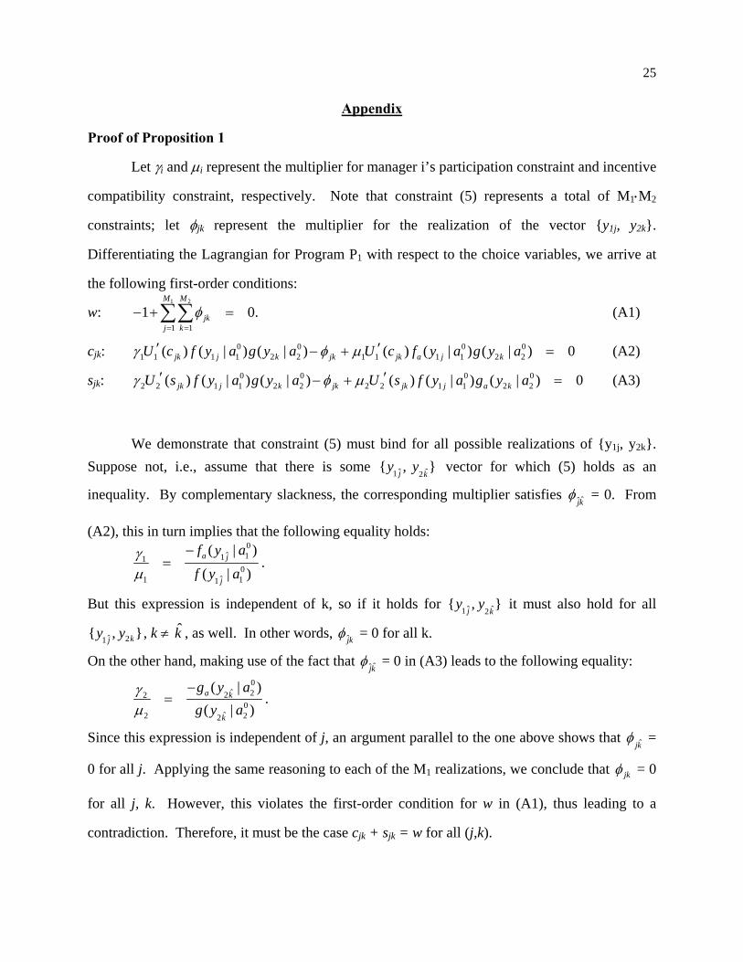
Proof of Proposition 1

Let γi and µi represent the multiplier for manager i’s participation constraint and incentive

compatibility constraint, respectively. Note that constraint (5) represents a total of M1⋅M2

constraints; let φjk represent the multiplier for the realization of the vector {y1j, y2k}.

Differentiating the Lagrangian for Program P1 with respect to the choice variables, we arrive at

the following first-order conditions:

w: (A1) 1 2

1 1

1M M

jkj k

φ= =

− + =∑∑ 0.

cjk: (A2) 0 0 0 01 1 1 1 2 2 1 1 1 1 2 2( ) ( | ) ( | ) ( ) ( | ) ( | ) 0jk j k jk jk a j kU c f y a g y a U c f y a g y aγ φ µ′ ′− + =

sjk: (A3) 0 0 0 02 2 1 1 2 2 2 2 1 1 2 2( ) ( | ) ( | ) ( ) ( | ) ( | ) 0jk j k jk jk j a kU s f y a g y a U s f y a g y aγ φ µ′ ′− + =

We demonstrate that constraint (5) must bind for all possible realizations of {y1j, y2k}. Suppose not, i.e., assume that there is some vector for which (5) holds as an

inequality. By complementary slackness, the corresponding multiplier satisfies

ˆ ˆ1 2{ , }j k

y y

ˆjkφ = 0. From

(A2), this in turn implies that the following equality holds: 0

ˆ 1110

ˆ1 11

( | )( | )a j

j

f y af y a

γµ

−= .

But this expression is independent of k, so if it holds for it must also hold for all

, k ≠ , as well. In other words,

ˆ ˆ1 2{ ,j k

y y }

}ˆ 21{ , kjy y k jkφ = 0 for all k.

On the other hand, making use of the fact that ˆjkφ = 0 in (A3) leads to the following equality:

0

ˆ 2220

ˆ2 22

( |( | )a k

k

g y ag y a

γµ

−=

).

Since this expression is independent of j, an argument parallel to the one above shows that ˆjkφ =

0 for all j. Applying the same reasoning to each of the M1 realizations, we conclude that jkφ = 0

for all j, k. However, this violates the first-order condition for w in (A1), thus leading to a

contradiction. Therefore, it must be the case cjk + sjk = w for all (j,k).

26

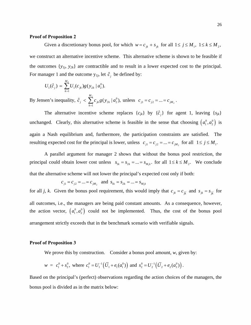
Proof of Proposition 2 Given a discretionary bonus pool, for which jk jkw c s= + for all 11 ,j M≤ ≤ 21 ,k M≤ ≤

we construct an alternative incentive scheme. This alternative scheme is shown to be feasible if

the outcomes {y1j, y2k} are contractible and to result in a lower expected cost to the principal. For manager 1 and the outcome y1j, let be defined by: ˆ jc

2

01 1 2

1

ˆ( ) ( ) ( | ).M

j jk kk

U c U c g y a=

= ∑ 2

,By Jensen’s inequality, unless 2

02 2

1

ˆ ( | )M

j jk kk

c c g y a=

< ∑ 21 2 ...j j jMc c c= = = .

The alternative incentive scheme replaces {cjk} by for agent 1, leaving {sˆ{ }jc jk}

unchanged. Clearly, this alternative scheme is feasible in the sense that choosing ( ) is

again a Nash equilibrium and, furthermore, the participation constraints are satisfied. The resulting expected cost for the principal is lower, unless

0 01 2,a a

21 2 ...j j jMc c c= = = for all 11 .j M≤ ≤

A parallel argument for manager 2 shows that without the bonus pool restriction, the principal could obtain lower cost unless

11 2 ... .k k Ms s s k= = = for all 21 k M .≤ ≤ We conclude

that the alternative scheme will not lower the principal’s expected cost only if both: and

21 2 ...j j jMc c c= = =11 2 ...k k Ms s s k= = =

for all j, k. Given the bonus pool requirement, this would imply that and ˆˆjk jkc c= ˆˆjk jk

s s= for

all outcomes, i.e., the managers are being paid constant amounts. As a consequence, however, the action vector, ( could not be implemented. Thus, the cost of the bonus pool

arrangement strictly exceeds that in the benchmark scenario with verifiable signals.

)0 01 2,a a

Proof of Proposition 3

We prove this by construction. Consider a bonus pool amount, w, given by: w = where 0 0

1 2 ,c s+ ( )0 1 01 1 1 1 1( )c U U e a−= + and ( )0 1 0

2 2 2 2 2( )s U U e a−= + .

Based on the principal’s (perfect) observations regarding the action choices of the managers, the

bonus pool is divided as in the matrix below:

27

Manager 2

02a Not 0

2a01a ( )0 0

1 2,c s ( )0 01 2,c s+ ∆ −∆

Manager 1 Not 01a ( )0 0

1 2,c s−∆ + ∆ ( )0 01 2,c s

For manager 1, the choice of is a dominant strategy provided: 0

1a

( ) ( )0 0 01 1 1 1 1 1 1 1 1( ) ( )U c e a U U c e a− ≡ ≥ −∆ − ;

and ( ) ( )0 0 0

1 1 1 1 1 1 1 1( ) ( )U c e a U c e a+ ∆ − ≥ − . For manager 2, the choice of is a dominant strategy provided: 0

2a

( ) ( )0 0 02 2 2 2 2 2 2 2 2( ) ( )U s e a U U s e a− ≡ ≥ −∆ − ;

and ( ) ( )0 0 0

2 2 2 2 2 2 2 2( ) ( ).U s e a U s e a+ ∆ − ≥ −

The above inequalities, when expressed as statements of the form g( ∆ ) ≥ 0, are all increasing

functions of . Therefore, provided the agents’ utilities can be made unboundedly negative, the

principal can always choose a sufficiently large positive

∆

∆ that satisfies all four inequalities.

Proof of Corollary 1

Consider the same bonus pool amount, w, as in the proof of Proposition 3 :

w = where 0 01 2 ,c s+ ( )0 1 0

1 1 1 1 1( )c U U e a−= + and ( )0 1 02 2 2 2 2( )s U U e a−= + .

The principal now allocates this pool according to the rule:

Manager 2

02a Not 0

2a01a ( )0 0

1 2,c s (w, 0) Manager 1 Not

01a (0, w) (0, w)

28

Given this ex-post distribution, the best manager 1 can do by choosing “Not ” is 01a

( )1 10 (U e− 1)a , while his worst utility from choosing is 01a 1U . As the latter is higher, it is a

strictly dominant strategy for manager 1 to choose .01a 23 We can therefore eliminate from

consideration any action choice other than . In response, manager 2 can either choose , for

a utility of

01a 0

2a

2U , or some action other than for a maximal utility of 02a ( )2 20 (U e a− 2 ) . Again, it is

strictly dominant for him to choose , implying that the game is dominance solvable, and the

unique outcome that survives the iterated elimination of strictly dominated strategies is

02a

( )0 01 2,a a .

For this choice vector, each manager receives his first-best wage, thus completing the proof.

Proof of Corollary 2

The proofs of Propositions 1, 2, and 3 extend in a relatively straightforward manner to a

setting with n managers. As for Corollary 1, consider, for notational convenience, a setting with

identical managers. Let w represent the total bonus pool amount needed to compensate all n

managers with their first-best wages, and consider the following asymmetric construction:

Manager Action Choice Payoff

1,2,3,..,n Obedient w/(n-m), where 0 ≤ m ≤ (n-1) is the total number of

disobedient managers.

1,2,..,(n-1) Disobedient 0.

n Disobedient 0, if there is at least one obedient manager;, otherwise. w

⎧⎨⎩

23 Note that we are making the innocuous implicit assumption that the manager has a non-trivial outside opportunity.

29

For all managers other than n, it is clear that obedience is a strictly dominant strategy. It is then

a Nash best response for manager n to also be obedient. The mechanism thus uniquely

implements first-best via the iterated elimination of strictly dominated strategies.24

Proof of Proposition 4

We start with a setting in which n managers are present. Let CR denote the compensation

given to a successful manager when a total of R agents (out of n) are successful. Given a bonus

pool of w, this implies that each unsuccessful manager receives Rw RCn R−−

. For convention, we

define C0 = 0; also note by symmetry that Cn = w/n.

We will find the following change of variables very useful:

Let CR = ( ) Rw n Rn

δ+ − .

This in turn implies that: .RR

w RC w Rn R n

δ−= −

−25

Let f1 and f2 represent a manager’s ex ante expected utility conditional on success and

failure, respectively. Then, in order to implement the symmetric action vector a = (a, a, …, a), the owner chooses the bonus pool size, w, and (n-1) variables, { }1 2 1, ,..., nδ δ δ − as solutions to the

following optimization problem:

Program P3: Minw, C1, C2, .., Cn-1

w

subject to: 1 2(1 ) ( )af a f e a U+ − − ≥ ; (A4)

and , (A5) 1 2 ( ) 0f f e a′− − =

where the quantities f1 and f2 are given by:

24 It is possible to derive stronger results. Even with limited liability constraints, it becomes easier to achieve implementation in dominant strategies as the number of managers increases. For example, if managers have power utilities (i.e., ), one can achieve obedience in dominant strategies at first-best cost provided 1( )U s sκκ −= 2.nκ ≥25 Note that, by construction, we have δn = 0.

30

f1 = 1

11

0

1(1 ) ( 1)

nR n R

RR

n wa a U n RR n

δ−

− −+

=

−⎛ ⎞ ⎛− + − −⎜ ⎟ ⎜⎝ ⎠⎝ ⎠

∑ ⎞⎟ ; (A6)

and f2 = 1

1

0

1(1 )

nR n R

RR

n wa a U RR n

δ−

− −

=

−⎛ ⎞ ⎛− −⎜ ⎟ ⎜⎝ ⎠⎝ ⎠

∑ ⎞⎟ . (A7)

Let the optimal solution to Program P3 be given by bonus pool and the (n-1)

adjustment variables,

ˆ nw

1 2 1ˆ ˆ ˆ, ,..., .nδ δ δ − It can be shown that the δR variables are all positive, and that

the expression RδR is increasing in R. Let 1f and 2f represent the optimal values for f1 and f2

that lead to constraints (A4) and (A5) being met as equalities.

We will now construct a solution with (n+1) managers that uses the average optimal

bonus pool with n managers, ˆ nwn

, but relaxes the participation constraint for each manager. We

use this to show that the optimal bonus pool with (n+1) managers must involve a strictly lower

per-capita bonus pool than the n-manager setting.

The key to the proof lies in the following construction:

Let 1 ˆ1

n nw wn n

+ =+

(for simplicity, we refer to this as wn

henceforth);

For R = 1, .., n, let 1( ) ( 1)ˆ

R Rn R R

n nˆRδ δ δ −

− −= + . (A8)

The formulation in (A8) identifies the precise way in which we will use the existing bonus pool

with n managers to construct a hypothetical bonus pool division with (n+1) managers. Our

proof proceeds in three parts.

Part 1: Under the construction in (A8), f1 is higher in the (n+1)-manager setting:

Proof: With n managers, equation (A6) lays out the value of f1. Expanding this

expression, the optimal value of f1, which we denote as 1f , equals the following: 2

1 11

1

1 ˆ(1 ) ( 1)n

n R n RR

R

nw wa U a a U n RRn n

δ−

− − −+

=

−⎛ ⎞⎛ ⎞ ⎛ ⎞+ − + − −⎜ ⎟⎜ ⎟ ⎜ ⎟⎝ ⎠ ⎝ ⎠⎝ ⎠

∑

31

11(1 ) ( 1)n wa U n

nδ− ⎛+ − + −⎜

⎝ ⎠⎞⎟ (A9)

With (n+1) managers, the corresponding expression for f1 looks as follows:

1

1 11

(1 ) ( ) (1 )n

n R n R nR

R

nw wa U a a U n R a U nRn n

wn

δ δ−

−+

=

⎛ ⎞⎛ ⎞ ⎛ ⎞ ⎛ ⎞+ − + − + − +⎜ ⎟⎜ ⎟ ⎜ ⎟ ⎜ ⎟⎝ ⎠ ⎝ ⎠ ⎝ ⎠⎝ ⎠

∑ (A10)

We want to show that (A10) exceeds (A9). Note that this is equivalent to showing that:

1

11

(1 ) ( )n

R n RR

R

n wa a U n RR n

−−

+=

⎛ ⎞ ⎛ ⎞− + −⎜ ⎟ ⎜ ⎟⎝ ⎠⎝ ⎠

∑ δ > 11(1 ) ( 1)n wa a U n

nδ− ⎛ ⎞− + −⎜ ⎟

⎝ ⎠

21 1

11

1 ˆ(1 ) (1 ) ( 1)n

n R n RR

R

nw wa a U a a U n RRn n

δ−

− − −+

=

−⎛ ⎞⎛ ⎞ ⎛ ⎞+ − + − + − −⎜ ⎟⎜ ⎟ ⎜ ⎟⎝ ⎠ ⎝ ⎠⎝ ⎠

∑ (A11)

Using the construction in (A8), the left-hand side of the inequality in (A11) can be re-written as:

1

11

1 ˆ ˆ(1 ) ( ) ( )n

R n RR R

R

n w n R Ra a U n R n RR n n n

δ δ−

−+

=

⎛ ⎞ ⎛ − −⎛ ⎞ ⎛ ⎞− + − + −⎜ ⎟ ⎜ ⎟ ⎜ ⎟⎜ ⎟⎝ ⎠ ⎝ ⎠⎝ ⎠⎝ ⎠∑ ⎞

= 12 1

2 1ˆ ˆ(1 ) ( 1)n w n nna a U nn n n

δ δ− ⎛ − −⎛ ⎞ ⎛ ⎞− + − +⎜ ⎟ ⎜ ⎟⎜ ⎟⎝ ⎠ ⎝ ⎠⎝ ⎠

⎞

+ 11

1 ˆ(1 )nn

w nna a Un n

δ−−

⎛ −⎛ ⎞− + ⎜ ⎟⎜ ⎟⎝ ⎠⎝ ⎠

⎞

+ 2

12

1 ˆ(1 ) ( ) ( )n

R n RR

R

n w n R Ra a U n R n RR n n n

ˆRδ δ

−−

+=

⎛ ⎞ ⎛ − −⎛ ⎞ ⎛ ⎞− + − + −⎜ ⎟ ⎜ ⎟ ⎜ ⎟⎜ ⎟⎝ ⎠ ⎝ ⎠⎝ ⎠⎝ ⎠∑ ⎞ (A12)

We will find it convenient to re-express the right side of the inequality in (A11) as below:

2

1 11 1

1

1ˆ ˆ(1 ) ( 1) (1 ) (1 ) ( 1)n

n n R n RR

R

nw w wa a U n a a U a a U n RRn n n

δ δ−

− − −+

=

−⎛ ⎞⎛ ⎞ ⎛ ⎞ ⎛− + − + − + − + − −⎜ ⎟⎜ ⎟ ⎜ ⎟ ⎜⎝ ⎠ ⎝ ⎠ ⎝⎝ ⎠

∑ ⎞⎟⎠

21 1

11

1 ˆ(1 ) ( 1)n

R n RR

R

n wa a U n RR n

δ−

+ − −+

=

−⎛ ⎞ ⎛ ⎞+ − + − −⎜ ⎟ ⎜ ⎟⎝ ⎠⎝ ⎠

∑

= 1 11 2ˆ ˆ(1 ) ( 1) ( 1) (1 ) ( 2)n nw wa a U n n a a U n

n nδ δ− −⎛ ⎞ ⎛− + − + − − + −⎜ ⎟ ⎜

⎝ ⎠ ⎝⎞⎟⎠

+ 1 11

ˆ(1 ) ( 1) (1 )n nn

w wa a U n a a Un n

δ− −−

⎛ ⎞ ⎛ ⎞− + − − +⎜ ⎟ ⎜ ⎟⎝ ⎠ ⎝ ⎠

32

+ 2

12

1 ˆ(1 ) ( 1)n

R n RR

R

n wa a U n RR n

δ−

−+

=

−⎛ ⎞ ⎛ ⎞− + − −⎜ ⎟ ⎜ ⎟⎝ ⎠⎝ ⎠

∑

+ 3

1 11

1

1 ˆ(1 ) ( 1)n

R n RR

R

n wa a U n RR n

δ−

+ − −+

=

−⎛ ⎞ ⎛− + − −⎜ ⎟ ⎜⎝ ⎠⎝ ⎠

∑ ⎞⎟ (A13)

To complete the proof, we compare carefully chosen sets of terms from (A12) and (A13).

We first compare the first term in (A12) to the sum of the first two terms in (A13). We find that

the former quantity is greater if (dividing through by 1(1 )nna a −− ), we have:

2 12 1ˆ ˆ( 1)w n nU n

n n nδ δ⎛ − − ⎞⎛ ⎞ ⎛ ⎞+ − +⎜ ⎟ ⎜ ⎟⎜ ⎟⎝ ⎠ ⎝ ⎠⎝ ⎠

> 1 21 1ˆ ˆ( 1) ( 2)w n wU n U nn n n n

δ δ−⎛ ⎞ ⎛ ⎞ ⎛ ⎞+ − + + −⎜ ⎟ ⎜ ⎟ ⎜ ⎟⎝ ⎠ ⎝ ⎠ ⎝ ⎠

.

But this follows from concavity of the utility function since the term on the left represents the

certainty equivalent of the lottery represented on the right hand side.

Similarly, to show that the second term in (A12) exceeds the sum of the third and fourth terms in

(A13), we divide through by 1(1 )nna a− − and find that we require:

11

nw nUn n

δ −

⎛ −⎛ ⎞+ ⎜ ⎟⎜ ⎟⎝ ⎠⎝ ⎠

⎞ > 11 1

nw n wU U

n n n nδ −

−⎛ ⎞ ⎛ ⎞ ⎛ ⎞+ +⎜ ⎟ ⎜ ⎟ ⎜ ⎟⎝ ⎠ ⎝ ⎠ ⎝ ⎠

,

which is again true from concavity.

Finally, we compare the last term in (A12) to the last two sets of sums in (A13). We do this for

each outcome R. For arbitrary R, dividing through by the expression nR

⎛ ⎞⎜ ⎟⎝ ⎠

(1 )R na a R−− , this

reduces the problem to one of demonstrating that::

11 ˆ ˆ( ) ( )R R

w n R RU n R n Rn n n

δ δ+

⎛ − −⎛ ⎞ ⎛ ⎞+ − + −⎜ ⎟ ⎜ ⎟⎜ ⎟⎝ ⎠ ⎝ ⎠⎝ ⎠

⎞ >

1( ) ˆ ˆ( 1) ( )R Rn R w R wU n R U n R

n n n nδ δ+

− ⎛ ⎞ ⎛ ⎞ ⎛+ − − + + −⎜ ⎟ ⎜ ⎟ ⎜⎝ ⎠ ⎝ ⎠ ⎝

⎞⎟⎠

Once again, for each R, the left hand side represents the certainty equivalent of the lottery on the

right, so the inequality holds. We have thus demonstrated that (A12) > (A13); under our

construction, the value of f1 is therefore higher in the (n+1) manager setting.

Part 2: Under the construction in (A8), f2 is higher in the (n+1)-manager setting:

Proof: Analogous to that of Part 1, and omitted for reasons of space.

33

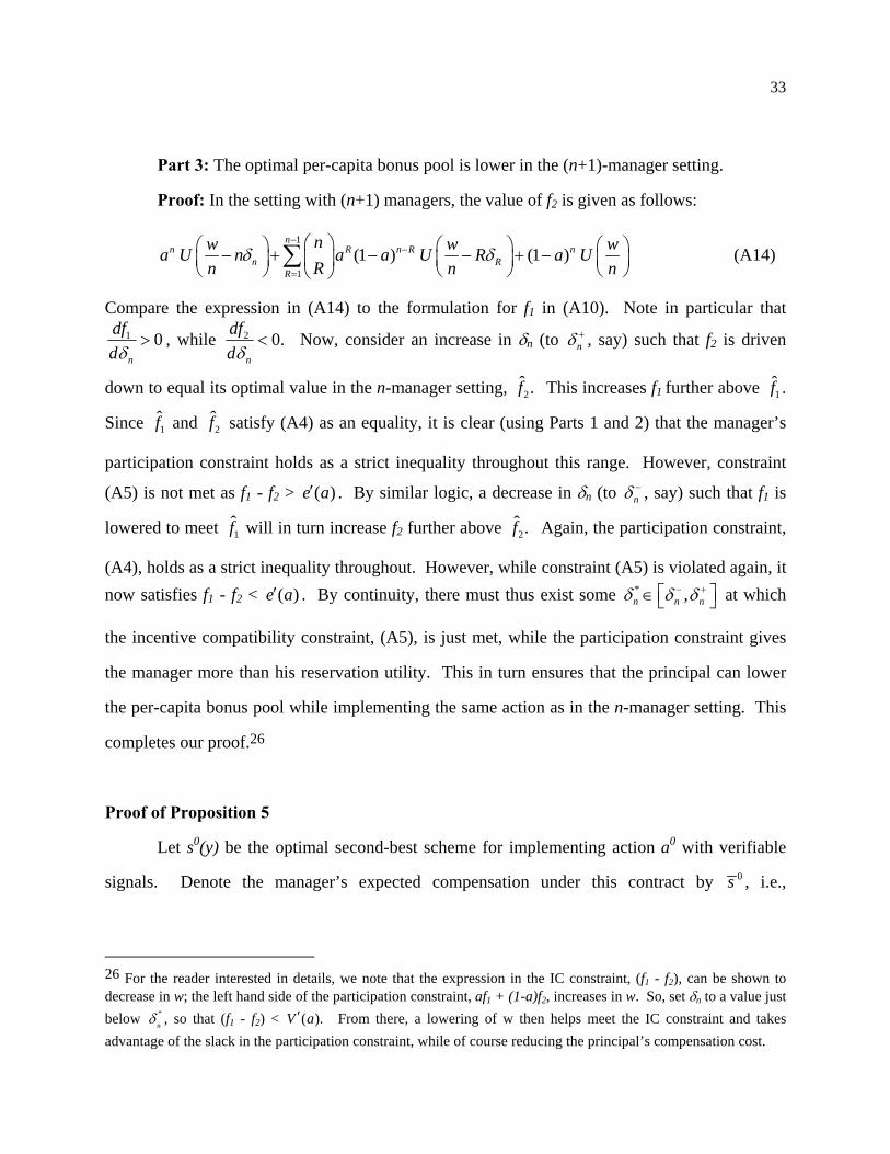
Part 3: The optimal per-capita bonus pool is lower in the (n+1)-manager setting.

Proof: In the setting with (n+1) managers, the value of f2 is given as follows:

1

1

(1 ) (1 )n

n R n Rn R

R

nw wa U n a a U R a URn n

δ δ−

−

=

⎛ ⎞⎛ ⎞ ⎛ ⎞ ⎛− + − − + −⎜ ⎟⎜ ⎟ ⎜ ⎟ ⎜⎝ ⎠ ⎝ ⎠ ⎝⎝ ⎠

∑ n wn⎞⎟⎠

(A14)

Compare the expression in (A14) to the formulation for f1 in (A10). Note in particular that 1 0n

dfdδ

> , while 2 0.n

dfdδ

< Now, consider an increase in δn (to nδ+ , say) such that f2 is driven

down to equal its optimal value in the n-manager setting, 2.f This increases f1 further above 1f .

Since 1f and 2f satisfy (A4) as an equality, it is clear (using Parts 1 and 2) that the manager’s

participation constraint holds as a strict inequality throughout this range. However, constraint

(A5) is not met as f1 - f2 > . By similar logic, a decrease in δ( )e a′ n (to nδ− , say) such that f1 is

lowered to meet 1f will in turn increase f2 further above 2.f Again, the participation constraint,

(A4), holds as a strict inequality throughout. However, while constraint (A5) is violated again, it now satisfies f1 - f2 < . By continuity, there must thus exist some ( )e a′ * ,n n nδ δ δ− +⎡∈ ⎣ ⎤⎦ at which

the incentive compatibility constraint, (A5), is just met, while the participation constraint gives

the manager more than his reservation utility. This in turn ensures that the principal can lower

the per-capita bonus pool while implementing the same action as in the n-manager setting. This

completes our proof.26

Proof of Proposition 5

Let s0(y) be the optimal second-best scheme for implementing action a0 with verifiable

signals. Denote the manager’s expected compensation under this contract by 0s , i.e.,

26 For the reader interested in details, we note that the expression in the IC constraint, (f1 - f2), can be shown to decrease in w; the left hand side of the participation constraint, af1 + (1-a)f2, increases in w. So, set δn to a value just below *

nδ , so that (f1 - f2) < From there, a lowering of w then helps meet the IC constraint and takes advantage of the slack in the participation constraint, while of course reducing the principal’s compensation cost.

( ).V a′

34

0 0[ ( ) | ]s E s y a= 0 . For a setting with n managers, consider the following compensation structure

for manager i, based on the vector of signal realizations for all n managers:

0 0 01 2

1( , ,... ) ( ) ( )( 1)i n i j

j is y y y s y s s y T

n ≠

⎡ ⎤= + − +⎢ −⎣ ⎦

∑ n⎥ , (A15)

where Tn is a constant (depending only on n). Note that (A15) defines a bonus pool for any n as:

1 21

( , ,... )n

i ni

s y y y=∑ 0 0 0

1 1

1( ) ( 1) ( )( 1)

n n

i ii i

s y n s n s y n Tn= =

= + ⋅ − − ⋅ +−∑ ∑ n⋅

( )0 .nn s T= ⋅ +

For notational convenience, we define a new random variable, 0 01 ( )( 1)

in j

j iz s s y

n ≠

.⎡ ⎤

= −⎢ ⎥−⎣ ⎦∑ %%

For all n, ’s support is contained by the interval i

nz% ( ) ( )0 0 0 0,Max Mins s s s⎡ ⎤− − −⎣ ⎦ , where 0Maxs and

0Mins represent the highest and lowest compensation levels under the second-best contract.

Consider manager i’s incentive under this bonus pool. If he conjectures that all other

managers choose the desired action a0, his optimization problem is given by:

( )0 0( ) ( ) | ,i

ia i n n iMax EU s y z T e a a −

⎡ ⎤+ + −⎣ ⎦% % ai i

i

.

Given a negative exponential utility function, this simplifies to:

( ) ( ) ( )0 0ˆ ˆ ˆ( | ) ( ) ( ) ( | )i

iin

i ia n n n i i i i

yz

Max exp k T exp k z g z exp k s y e a f y a−

⎧ ⎫⎡ ⎤ ⎡ ⎤⎪ ⎪⎡ ⎤− − ⋅ ⋅ − − ⋅ ⋅ − − ⋅ −⎢ ⎥⎨ ⎬⎢ ⎥⎣ ⎦⎢ ⎥⎪ ⎪⎣ ⎦⎣ ⎦⎩ ⎭∑ ∑a .

Now, let Tn be chosen by the owner as follows:

( ) 01 ˆ ( | )ˆ in

i in n

z

T ln exp k z g zk −

⎡ ⎤= ⋅ − ⋅⎢

⎢ ⎥⎣ ⎦∑ an i ⎥ . (A16)

The first two terms in the manager’s expected utility then cancel, implying that his utility, and

choice of action, are determined solely by the second-best contract. He will therefore choose the

desired action, a0, and obtain his reservation utility, independently of n.

35

Since , Jensen’s inequality applied to the right-hand side in (A16) yields the

implication that T

( ) 0inE z =%

n > 0. As one would expect, the bonus pool construction, which requires the owner to set aside an average of ( 0

ns T+ ) per manager, is thus costlier than the benchmark

average cost with verifiable signals ( )0 .s To complete the proof, note that the variable

represents the difference between the expected value and the realized mean level of

compensation, in a sample with

inz%

( 1)n − i.i.d draws. From the weak law of large numbers, we

know that in probability. Using the continuity of the exponential function, it then

follows (see, e.g., the proof of Theorem 4.4.5 in Chung 1974) that:

0inz →%

( )( ) ( )( )1 1ˆ ˆ 0 0ˆ ˆi

n nT ln E exp k z ln E exp kk k

⎡ ⎤ ⎡= − ⋅ → − ⋅⎢ ⎥ ⎢⎣ ⎦ ⎣% .⎤ =⎥⎦

.n →∞

The performance of the bonus pool therefore converges to benchmark performance as

Proof of Proposition 6: Stochastic independence among all error terms immediately implies for all 0iju = .i j≠

The principal’s cost in P2 therefore reduces to:

C(n) = 2 2 2 2{ , }

1 1,

ij ij

n n

u w i i ii j iji j

Min k u w= =

⎡ ⎤⋅ ⋅ + ⋅⎢ ⎥⎣ ⎦

∑ ∑σ η

subject to the incentive and bonus pool constraints. Substituting the incentive constraint into the

objective function, the optimization problem becomes:

( )22 0 2

{ }1 1

( ) . ,ij

n n

w i i i i i ii ji j

2ijMin k e a m w w

= =

⎡ ⎤′⋅ ⋅ − + ⋅⎢ ⎥⎣ ⎦

∑ ∑σ η

subject to: for 11

0n

iji

w=

=∑ .j n≤ ≤

The first-order conditions with respect to wii are:

( )2 0 22 ( )i i i i i ii i i ii ik e a m w m wσ η⎡ ′⋅ ⋅ − ⋅ − ⋅ ⋅ + ⋅ + =⎢⎣0λ⎤

⎥⎦ (A17)

and for wij one obtains:

36

22 0i j ij jk wη λ⋅ ⋅ ⋅ + = .

Clearly, wii > 0 and wji < 0 for j i≠ .27 Therefore, λi > 0. To conclude that

* 0 2

* 0 2ii ii i i

ii ii i

w w mu u

ση⋅

< ≡ , (A18)

we note that the benchmark solution of

2 0 2 0

0 02 2 2 2 2 2

( ) ( );i i i i i i iii ii

i i i i i i

m e a e aw um mσ ησ η σ

′ ′⋅ ⋅ ⋅= =

⋅ + ⋅ +η

*

would solve the first-order condition in (A17) if λi = 0. Since solve (A17) for λ* ,ii iiw u i > 0, the

inequality in (A18) follows immediately. That completes the proof of part i).

ii) With n-identical agents, the principal chooses { },ij iju w ,

w

to minimize:

2 2 2 2

11

n n

ii ijji

uσ η==

⎡ ⎤⎡ ⎤⎢ ⎥⎢ ⎥⋅ + ⋅ ∑⎢ ⎥⎢ ⎥⎣ ⎦⎣ ⎦

∑ (A19)

subject to: 1

0,n

iji

w=∑ =

and ,ii iim w u e′⋅ + = where . For any given ( , the principal chooses ( )0e e a′ ′≡ )11, , nnw wK { }ij i j

w≠

so as to minimize

the total bonus pool variance associated with . That implies: iiw1

1ji iiw wn

= − ⋅−

,

and (A19) reduces to: ( ) ( )2

22 2 2

11

1

nii

ii iii

we m w w nn

σ η=

⎛ ⎞⎡ ⎤⎛ ⎞⎡ ⎤′⎜ ⋅ − ⋅ + ⋅ + − ⋅ ⎟⎢ ⎥⎜ ⎟⎣ ⎦⎜ ⎟−⎝ ⎠⎢ ⎥⎣ ⎦⎝ ⎠∑ .

The corresponding first-order conditions yield:

27 The only reason to choose is because w0jiw ≠ ii > 0. If wii = 0, then wji = 0 and λi = 0, violating the first-order

condition in (A17).

37

( )2

*

2 2 2

1

iim ew n nm

n

σ

σ η

′⋅ ⋅=

⋅ + ⋅−

; and ( )2

*

2 2 2

1

1

ii

n enu n nm

n

η

σ η

′⋅ ⋅−=

⋅ + ⋅−

.

Thus, the ratio of the optimal coefficients is: ( )( )

* 2

*

1ii

ii

w n n mu n n

ση 2

⎡ ⎤−= ⋅ ⋅⎢ ⎥

⎣ ⎦, proving the claim.

Proof of Corollary to Proposition 6: Let denote the optimal coefficients on and , respectively, when

there are -identical agents. As shown in Proposition 6,

( ( ) , ( )ii iiu n w n∗ ∗ )n

ix iy

( ) ( ) 11ji iiw n w n

n∗ ∗= − ⋅

−

Thus the principal’s per capita cost is:

( ) ( )( ) ( )( )2 22 2

1ii ii

C n nk u n w nn n

∗ ∗⎡ ⎤⎛ ⎞= ⋅ ⋅ + ⋅ ⋅⎜ ⎟⎢ ⎥−⎝ ⎠⎣ ⎦σ η

It will be convenient to define:

( ) ( )( ) ( )( )2 22 21 11 ii ii

C n nk u n w nn n

+∗ ∗+ ⎡ +⎛ ⎞≡ ⋅ ⋅ + ⋅ ⋅⎜ ⎟⎢ ⎥+ ⎝ ⎠⎣ ⎦

σ η ⎤

)1

.

By definition, . The first claim then follows by observing that: ( ) (1C n C n+ + > +

( ) ( )11

C n C nn n

+ +>

+,

since: 1

1n n

n n+

>−

.

To establish the second part, we note that ( ) oii iiu n u∗ → and that ( ) o

ii iiw n w∗ → as , since in

the benchmark setting, and

n → ∞

0oii iiu e m w′= − ⋅ 2 2o o

ii iiw m uη σ⋅ = ⋅ ⋅ .

Taking the limit of the per-capita cost for large values of n, we obtain:

( ) ( ) ( )2 22 2o oii ii

C nk u w

nσ η⎡ ⎤→ ⋅ ⋅ + ⋅⎢ ⎥⎣ ⎦

.

38

To show that ( )*

C nC

n− has order 1

n, it suffices to note that:

( )( ) ( )2 2 1oii iiu n u O

n∗ ⎛ ⎞− ∈ ⎜ ⎟

⎝ ⎠ and ( )( ) ( )2 2 1o

ii iiw n w On

∗ ⎛ ⎞− ∈ ⎜ ⎟⎝ ⎠

.

Both of these claims follow directly after substitution of the expressions for ( ) ( ) 0, ,ii ii iiu n w n u∗ ∗ ,

i

2

and , as given in the proof of Proposition 6. 0iiw

Proof of Proposition 7: It is clear that . Substituting the bonus pool and incentive constraints into the

objective function in (11), the principal’s cost then becomes:

0,iju j= ≠

( ) ( )2 22 2 211 22 11 22 11 222 2k e m w e m w w w w wσ η θ⎡ ⎤⎡ ⎤′ ′ ⎡ ⎤⋅ ⋅ − ⋅ + − ⋅ + ⋅ ⋅ + − ⋅ ⋅ ⋅⎣ ⎦⎣ ⎦⎣ ⎦

. (A20)

We note that the objective function in (A20) is convex in ( )11 22,w w , because the matrix oΣ is

positive semi-definite. Thus, the first-order conditions are necessary and sufficient for a cost

minimum. The corresponding first-order conditions are:

( ) [ ]2 211 11 222m e m w w w ,σ η′⋅ ⋅ − ⋅ = ⋅ ⋅ − ⋅θ (A21)

and ( ) [ ]2 222 22 112m e m w w w .σ η′⋅ ⋅ − ⋅ = ⋅ ⋅ − ⋅θ (A22)

Solving (A21) and (A22) yields: ( )

2*

2 2 2( )2 1ii

m ewm

σθσ η θ

′⋅ ⋅=

⋅ + ⋅ ⋅ −.

From the incentive constraints, we then obtain: ( )( )

2*

2 2 2

2 1( )

2 1ii

eu

mη θ

θσ η θ

′⋅ ⋅ − ⋅=

⋅ + ⋅ ⋅ −.

Therefore, the ratio of the optimal coefficients satisfies:

( ) ( )* 2

* 2

( ) 1 .( ) 2 1

iii

ii

wR mu

θ σθθ η θ

= = ⋅ ⋅⋅ −

(A23)

39

Claims (ii) and (iii) follow immediately from inspection of (A23). To establish claim (i), we

note that by the Envelope Theorem:

( ) ( ) ( )* * 211 222 4C k w wθ θ θ

θ∂

= − ⋅ ⋅ ⋅ ⋅ <∂

0η ,

thus completing the proof of Proposition 7.

Proof of Proposition 8:

Due to the bonus pool requirement ( 11 21 22 12 0w w w w+ = + = ), the risk premium becomes:

( ) ( )2 22 2 2 2 2 2 2 2 2 211 11 11 22 22 22 22 11k u w u w u w u wσ η η σ η⎡ ⎤⋅ ⋅ + + ⋅ + ⋅ + ⋅ + + ⋅ + ⋅⎣ ⎦η

2

,

where 2 2 .σ η ζ= + To minimize this premium subject to the incentive constraints,

, the principal will set , irrespective of the values of ( )ii iim u w e′⋅ + = 0iiu > 2σ and 2η . This

follows directly from observing that: 2 2

2 2 2ii ii ii ii

e eu u u um m

2σ η η′ ′⎛ ⎞ ⎛ ⎞⋅ + + − ⋅ + − ⋅⎜ ⎟ ⎜ ⎟

⎝ ⎠ ⎝ ⎠

is always minimized by some 0.iiu >

40

References

Baiman, S., and M. Rajan. 1995. The informational advantages of discretionary bonus schemes. The Accounting Review 70 (October): 557-579. Baker, G., R. Gibbons, and K. Murphy. 1994. Subjective performance measures in optimal incentive contracts. Quarterly Journal of Economics 109 (November): 1125-1156. Baldenius, T., N. Melumad, and A. Ziv. 2002. Monitoring in multiagent organizations. Contemporary Accounting Research 19 (Winter): 483-511. Banker, R., and S. Datar. 1989. Sensitivity, precision, and linear aggregation of signals for performance evaluation. Journal of Accounting Research 27 (Spring): 21-39. Bernheim, B., and M. Whinston. 1998. Incomplete contracts and strategic ambiguity. American Economic Review 88 (September): 902-932. Brown, C. 1990. Firms’ choice of method of pay. Industrial and Labor Relations Review 43 (February): 165S-182S. Bull, C. 1987. The existence of self-enforcing implicit contracts. The Quarterly Journal of Economics 102 (February): 147-159. Christensen, P., G. Feltham, and F. Sabac. 2003. Dynamic incentives and responsibility accounting. Journal of Accounting and Economics 35, 423-436. Chung, K. L. 1974. A Course in Probability Theory. San Diego, CA: Academic Press. Dye, R. 1985. Costly contract contingencies. International Economic Review 26 (February): 233-250. Feltham, G., and J. Xie. 1994. Performance measure congruity and diversity in multi-task principal/agent relations. The Accounting Review 69 (July): 429-453. Fisher, J., L. Maines, S. Peffer, and G. Sprinkle. 2003. An experimental investigation of objective and subjective performance evaluation. Working paper, Indiana University. Fox, H. 1979. Top executive bonus plans: A research report from the Conference Board. New York, NY: The Conference Board. Gibbs, M., K. Merchant, K, W. Van der Stede, and M. Vargus. 2004. Determinants and effects of subjectivity in incentives. The Accounting Review 79 (April): 409-436.

41

Grossman, S., and O. Hart. 1983. An analysis of the principal-agent problem. Econometrica 51 (January): 7-45. Hayes, R., and S. Schaefer. 2000. Implicit contracts and the explanatory power of top executive compensation for future performance. RAND Journal of Economics 31 (Summer): 273-293. Holmstrom, B. 1979. Moral hazard and observability. Bell Journal of Economics 10 (Spring): 74-91. Holmstrom, B. 1982. Moral hazard in teams. Bell Journal of Economics 13 (Autumn): 324-340. Holmstrom, B., and P. Milgrom. 1991. Multitask principal-agent analyses: Incentive contracts, asset ownership, and job design. Journal of Law, Economics and Organizations 7: 24-52. Huddart, S., and P. Liang. 2003. Accounting in partnerships. American Economic Review 93 (May): 410-414. Huddart, S., and P. Liang. 2004. Profit sharing and monitoring in partnerships. Working paper, Pennsylvania State University. Indjejikian, R., D.J. Nanda. 1999. Dynamic incentives and responsibility accounting. Journal of Accounting and Economics 27, 177-201. Jewitt, I. 1988. Justifying the first-order approach to principal-agent problems. Econometrica 56 (September): 1177-1190. Laffont, J., and D. Martimort. 2001. The theory of incentives: the principal-agent model. Princeton University Press. Levin, J. 2003. Relational incentive contracts. American Economic Review 93 (June): 835-847. MacLeod, W. 2003. Optimal contracting with subjective evaluation. American Economic Review 93 (March): 216-240. MacLeod, W., and D. Parent. 1999. Jobs characteristics and the form of compensation. Research in Labor Economics 18: 231-59. Melumad, N., D. Mookherjee, and S. Reichelstein. 1997. Contract complexity, incentives and the value of delegation. Journal of Economics and Management Strategy 6 (Summer): 257-289. Rajan, M., and B. Sarath. 1997. The value of correlated signals in agencies. RAND Journal of Economics 28 (Spring): 150-167. Sinclair-Desgagne, B. 1994. The first-order approach to multi-signal principal-agent problems. Econometrica 62 (March): 459-465.

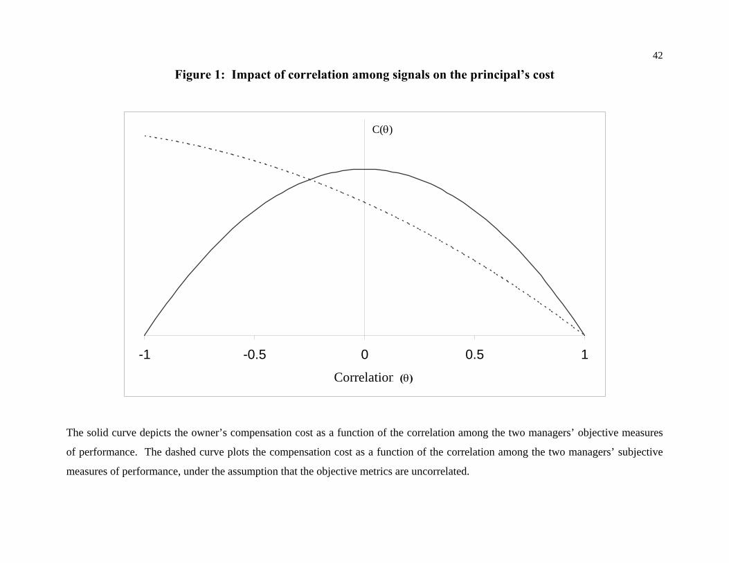
42

Figure 1: Impact of correlation among signals on the principal’s cost

-1 -0.5 0 0.5 1

Correlation

C(θ)

(θ)

The solid curve depicts the owner’s compensation cost as a function of the correlation among the two managers’ objective measures

of performance. The dashed curve plots the compensation cost as a function of the correlation among the two managers’ subjective

measures of performance, under the assumption that the objective metrics are uncorrelated.