study on flow characteristics of supersonic moist air...
TRANSCRIPT
Study on Flow Characteristics of
Supersonic Moist Air Impinging
Jets
Miah Md. Ashraful Alam
Graduate School of Science & Engineering
Saga University, Japan
A thesis submitted for the degree of
Doctor of Philosophy
24 March, 2011

2

I would like to dedicate this dissertation to my loving wife and son ...........
Acknowledgements
First, I would like to express my sincere gratitude to my supervisor, Prof.
Toshiaki Setoguchi, who has been a continuous source of encouragement.
Particularly, I am very grateful for his motivating and stimulating approach,
which helped me in developing my own vision for the PhD research. He
continuously provided me with inspiration and solicitude for all aspects of
my social life. Further, as often stated, the atmosphere in the working
environment is also very important. In this respect, I am very grateful for
his friendly and concerned attitude, which was definitely of great help in
difficult moments.
I would also like to thank my co-supervisor, Prof. Shigeru Matsuo, for the
valuable discussions, which led me to really understand and grasp CFD tech-
niques, and for the critical remarks and corrections, which have improved
the quality of this thesis considerably.
Prof. Miyara and Dr. Kinoue, the members of the committee, are grate-
fully acknowledged for their time and effort in my research program and
the reviewing of this thesis. Their critical remarks and suggestions have
improved the readability of the thesis considerably.
Understanding the code and clearing up the problems which sometimes
came out was just not possible without the help and expertise of Dr. Tanaka.
I’ve learned a lot about numerical techniques from him and I also benefited
from his some useful discussions during the first year. I would also like to
thank my lab-mates particularly Mr. Nishizaki, Mr. Kim, Mr. Umezaki,
Mr. Nakano, Mr. Inoue, Mr. Arata and Mr. Nagao for their help and
cooperation during my study.
As always the case in experimental work, a fundamental key to its success is
represented by the help and support of co-workers. The experimental work
could not succeed without the substantial support from my lab mates, Mr.
Koyama and Mr. Tokuda.
I have greatly enjoyed every single day during my study at Saga Univer-
sity and living in Japan. I have always been very proud of having the
opportunity to do my research in the laboratory of Environmental Fluids
Engineering, and I can say with no doubt it was one of the best experiences
of my life, so far.
I’m grateful to my two younger sisters, Rita and Rony, my dear father and
my late mother, my parents-in-law, Noorun Nahar and Abu Bakare for their
utmost care, love and support. I owe a tremendous debt to my wife, Nasrin
Nahar Shapla, who understood and supported me throughout all the time.
I feel deep sense of gratitude for her love and patience during the study
period, and efforts in maintaining our nice family life beyond her study.
Some of the best experiences that we lived through in this period were the
birth of our son Arham Zulkarnain Yafi, who provided an additional and
joyful dimension to our life mission. Shapla and Yafi cheered me up and
brought me new energy to face every new day.
Lastly, I would like to express my gratitude and thanks to all faculty mem-
bers of the Department of Advanced Systems Control Engineering and Me-
chanical Engineering. The financial support in the form of Mobukagakusho
scholarship, MEXT, Government of Japan, and the Sasagawa research grant
from the Japan Science Society to carry out this research work is gratefully
acknowledged.
Miah Md. Ashraful Alam
Saga, March 2011
Abstract
Supersonic impinging jets are characterized by a strong coupling between
the flow and acoustic fields with a self-induced feedback mechanism. This
self-induced oscillatory flow make thermal and mechanical loading more se-
vere and produces severe noise at discrete frequencies, which may cause
sonic fatigue of the structures and also may damage various instruments
and equipments. These loads are also accompanied by dramatic lift loss,
severe ground erosion, etc. Despite the simple geometry, the flow structure
of a supersonic impinging jet is rather complex; it contains mixed super-
sonic and subsonic regions, and involves interaction of shock and expansion
waves with jet shear layers. The feedback loop begins with the formation
of turbulence structures within the jet shear layer. These structures grow
and convect downstream where they interact with the obstacle, and create
acoustic waves. However, in actual jet flows, the working gas may contain
condensable gas such as steam or moist air. In these cases, non-equilibrium
homogeneous condensation may occur at the region between nozzle exit and
an object. The jet flow with non-equilibrium condensation may be quite
different from that without condensation. Moreover, no considerable work
has been done to study the effect of non-equilibrium homogeneous conden-
sation on flow characteristics of supersonic impinging jets, so far. Therefore,
the focus of the present numerical investigation is to investigate the effect
of non-equilibrium homogeneous condensation on the flow characteristics
of under-expanded supersonic impinging jets. Both experiments and nu-
merical investigations have been conducted on the supersonic moist air jets
to validate the numerical code, and the predicted results were compared
with the experimental data. Experiments have also been conducted on the
supersonic impinging jets, and the results were compared with the numer-
ically predicted data. In addition, a literature survey revealed that very
few researches have only been conducted on the impinging jets onto cavity,
so far, and most studies on impinging jets onto cavity have only been con-
cerned with subsonic flow. However, the study on the supersonic impinging
jets onto the cylindrical cavity has not yet been performed, so far. There-
fore, another objective of the present study is to numerically investigate
the flow characteristics of supersonic impinging jets onto cylindrical cavity,
and the effect of non-equilibrium homogeneous condensation on their flow
characteristics.
Both the experiment and computational works have been conducted to in-
vestigate the flow characteristics of under-expanded supersonic moist air
impinging jets on flat plate. In supersonic moist air impinging jets, the
amplitude of pressure on jet axis becomes smaller with an increase in the
initial degree of supersaturation. The amplitude of pressure fluctuation
changes with time, and the time averaged pressure at center of the plate is
affected by the pressure ratio and position of the plate. However, pressures
behind the Mach disk and at center of the impinging plate are decreased
due to the effect of non-equilibrium condensation. The amplitude of surface
pressure oscillation and peaks of the power spectrum density of the pres-
sure at center of the impinging plate are reduced in the case of moist air
impinging jets. Moreover, in case with non-equilibrium condensation the
jet boundary expands outward, and the magnitude of entrainment velocity
which corresponds to the reduction of lift loss is reduced.
Numerical simulations have also been done to investigate the flow charac-
teristics of under-expanded supersonic impinging jets onto the cylindrical
cavity, and the effect of non-equilibrium condensation on their flow proper-
ties. The cylindrical cavity has strong influence on the flow characteristics
especially on the flowfield oscillation. The increase in the nozzle-to-cavity
distances significantly influences the jet flowfield particularly increase the
amplitude of pressure fluctuations. However, the oscillation frequency de-
creases with the increase in the cavity height. Moreover, the large cavity
diameters increase the amplitude of pressure fluctuations. In case of moist
air jets, the non-equilibrium condensation has a significant influence on the

jet flowfield. The occurrence of non-equilibrium condensation increases the
flowfield oscillation except for the cases with large cavity diameter (1.5De).
In cases with large cavity diameters (1.5De), the amplitude of pressure os-
cillation decreases at a lower degree of non-equilibrium condensation, and it
increases again at higher value of initial degree of supersaturation. The oc-
currence of non-equilibrium condensation increases the amplitude of surface
pressure oscillation and peaks of the power spectrum density of pressure at
center of the cavity bottom wall.
Contents
Contents vii
List of Tables xiii
List of Figures xv
Nomenclature xx
1 Introduction 1
1.1 Motivation . . . . . . . . . . . . . . . . . . . . . . . . . . . . . . . . . . 1
1.2 Background . . . . . . . . . . . . . . . . . . . . . . . . . . . . . . . . . . 5
1.2.1 Supersonic free jet . . . . . . . . . . . . . . . . . . . . . . . . . . 5
1.2.2 Flowfield of impinging jet . . . . . . . . . . . . . . . . . . . . . . 8
1.3 Literature review . . . . . . . . . . . . . . . . . . . . . . . . . . . . . . . 14
1.4 Objectives . . . . . . . . . . . . . . . . . . . . . . . . . . . . . . . . . . . 23
1.5 Outline of the dissertation . . . . . . . . . . . . . . . . . . . . . . . . . . 24
2 Condensation phenomena 31
2.1 Introduction . . . . . . . . . . . . . . . . . . . . . . . . . . . . . . . . . . 31
2.2 Condensation & nucleation . . . . . . . . . . . . . . . . . . . . . . . . . 33
2.2.1 Condensation shock wave: a historical review . . . . . . . . . . . 37
2.2.2 Condensation in a supersonic nozzle . . . . . . . . . . . . . . . . 38
2.2.3 Fundamental definitions: amount of state . . . . . . . . . . . . . 40
2.2.4 Condensation shock wave: a detail about generation physics . . . 42
2.2.5 Flowfield oscillations by unsteady condensation shock wave . . . 45
2.3 Thermodynamics of condensation . . . . . . . . . . . . . . . . . . . . . . 46
2.3.1 Mixture of gases with no condensation . . . . . . . . . . . . . . . 47
vii
CONTENTS
2.3.2 Mixture of gases with condensation . . . . . . . . . . . . . . . . . 48
2.4 Homogeneous nucleation . . . . . . . . . . . . . . . . . . . . . . . . . . . 50
2.4.1 Generation of the cluster . . . . . . . . . . . . . . . . . . . . . . 51
2.4.2 Critical Cluster . . . . . . . . . . . . . . . . . . . . . . . . . . . . 55
2.4.3 Frenkel’s nucleation rate . . . . . . . . . . . . . . . . . . . . . . . 55
2.5 Droplet Growth . . . . . . . . . . . . . . . . . . . . . . . . . . . . . . . . 58
2.5.1 Growth rate of the cluster . . . . . . . . . . . . . . . . . . . . . . 58
2.5.2 Rate of condensation . . . . . . . . . . . . . . . . . . . . . . . . . 61
2.6 Change of entropy due to condensation . . . . . . . . . . . . . . . . . . . 62
2.7 Conclusion . . . . . . . . . . . . . . . . . . . . . . . . . . . . . . . . . . 63
3 Physical and mathematical modeling 73
3.1 Introduction . . . . . . . . . . . . . . . . . . . . . . . . . . . . . . . . . . 73
3.2 Governing equations . . . . . . . . . . . . . . . . . . . . . . . . . . . . . 73
3.2.1 Governing equations in Cartesian coordinates . . . . . . . . . . . 74
3.2.2 Transformation to generalized coordinates . . . . . . . . . . . . . 81
3.2.2.1 Obtaining the Metrics . . . . . . . . . . . . . . . . . . . 82
3.2.2.2 Applying the Transformation . . . . . . . . . . . . . . . 83
3.3 Turbulence modeling . . . . . . . . . . . . . . . . . . . . . . . . . . . . . 87
3.3.1 Eddy-viscosity model . . . . . . . . . . . . . . . . . . . . . . . . . 89
3.3.1.1 The basic equations of turbulence . . . . . . . . . . . . 89
3.3.1.2 Reynolds averaging . . . . . . . . . . . . . . . . . . . . 90
3.3.1.3 Mass averaging . . . . . . . . . . . . . . . . . . . . . . . 91
3.3.1.4 Reynolds-averaged Navier-Stokes equations . . . . . . . 92
3.3.1.5 Eddy-viscosity hypothesis . . . . . . . . . . . . . . . . . 94
3.3.2 Modified k −R turbulence model . . . . . . . . . . . . . . . . . . 96
3.3.2.1 Transport equations . . . . . . . . . . . . . . . . . . . . 97
3.3.2.2 Initial and boundary conditions . . . . . . . . . . . . . 102
3.4 Conclusion . . . . . . . . . . . . . . . . . . . . . . . . . . . . . . . . . . 102
4 Numerical modeling 103
4.1 Introduction . . . . . . . . . . . . . . . . . . . . . . . . . . . . . . . . . . 103
4.2 TVD scheme . . . . . . . . . . . . . . . . . . . . . . . . . . . . . . . . . 104
4.2.1 Linear system (scalar scheme) . . . . . . . . . . . . . . . . . . . . 106
viii
CONTENTS
4.2.2 Extension to a system of equations . . . . . . . . . . . . . . . . . 107
4.3 Riemann solver . . . . . . . . . . . . . . . . . . . . . . . . . . . . . . . . 115
4.3.1 Roe’s approximate Riemann solver (Roe average method) . . . . 116
4.3.2 Flux vector splitting (FVS) method . . . . . . . . . . . . . . . . 118
4.4 Jacobian matrices and eigenvectors . . . . . . . . . . . . . . . . . . . . . 119
4.4.1 In case of no condensation . . . . . . . . . . . . . . . . . . . . . . 119
4.4.2 In case with condensation . . . . . . . . . . . . . . . . . . . . . . 121
4.4.3 For k −R turbulence model . . . . . . . . . . . . . . . . . . . . . 124
4.5 Time integration . . . . . . . . . . . . . . . . . . . . . . . . . . . . . . . 126
4.5.1 Time splitting method . . . . . . . . . . . . . . . . . . . . . . . . 126
4.5.2 Calculation of time step size . . . . . . . . . . . . . . . . . . . . . 128
4.6 Convergence criterion . . . . . . . . . . . . . . . . . . . . . . . . . . . . 129
4.7 Conditions for numerical simulation . . . . . . . . . . . . . . . . . . . . 129
4.8 Conclusion . . . . . . . . . . . . . . . . . . . . . . . . . . . . . . . . . . 130
5 Experimental works 131
5.1 Experimental setup . . . . . . . . . . . . . . . . . . . . . . . . . . . . . . 131
5.2 Pressure measuring system . . . . . . . . . . . . . . . . . . . . . . . . . 133
5.3 Schlieren optical system . . . . . . . . . . . . . . . . . . . . . . . . . . . 134
6 Underexpanded supersonic moist air jets 137
6.1 Introduction . . . . . . . . . . . . . . . . . . . . . . . . . . . . . . . . . . 137
6.2 Computational domain & grids system . . . . . . . . . . . . . . . . . . . 137
6.3 Initial & boundary conditions . . . . . . . . . . . . . . . . . . . . . . . . 138
6.4 Numerical analysis . . . . . . . . . . . . . . . . . . . . . . . . . . . . . . 139
6.5 Results & discussion . . . . . . . . . . . . . . . . . . . . . . . . . . . . . 139
6.5.1 Comparisons of predicted iso-density contours with schlieren images139
6.5.2 Flow properties of jets . . . . . . . . . . . . . . . . . . . . . . . . 140
6.5.3 Jet and shock structures . . . . . . . . . . . . . . . . . . . . . . . 141
6.6 Conclusion . . . . . . . . . . . . . . . . . . . . . . . . . . . . . . . . . . 143
ix
CONTENTS
7 Supersonic impinging moist air jets on flat plate 155
7.1 Introduction . . . . . . . . . . . . . . . . . . . . . . . . . . . . . . . . . . 155
7.2 Computational domain & grids system . . . . . . . . . . . . . . . . . . . 155
7.3 Initial & boundary conditions . . . . . . . . . . . . . . . . . . . . . . . . 156
7.4 Numerical analysis . . . . . . . . . . . . . . . . . . . . . . . . . . . . . . 157
7.5 Results & discussion . . . . . . . . . . . . . . . . . . . . . . . . . . . . . 158
7.5.1 Check for grid independency . . . . . . . . . . . . . . . . . . . . 158
7.5.2 Comparison with experimental results . . . . . . . . . . . . . . . 158
7.5.3 Flow structure of impinging jets . . . . . . . . . . . . . . . . . . 158
7.5.4 Flow properties of dry air impinging jets . . . . . . . . . . . . . . 160
7.5.5 Effect of non-equilibrium condensation on impinging jets . . . . . 168
7.5.5.1 Flow properties of moist air impinging jets . . . . . . . 168
7.5.5.2 Jet and shock structure of moist air impinging jets . . . 172
7.5.5.3 Acoustic wave properties . . . . . . . . . . . . . . . . . 177
7.5.5.4 Lift loss . . . . . . . . . . . . . . . . . . . . . . . . . . . 177
7.6 Conclusion . . . . . . . . . . . . . . . . . . . . . . . . . . . . . . . . . . 178
8 Supersonic impinging jets onto cylindrical cavity 183
8.1 Introduction . . . . . . . . . . . . . . . . . . . . . . . . . . . . . . . . . . 183
8.2 Computational domain & grids system . . . . . . . . . . . . . . . . . . . 183
8.3 Initial & boundary conditions . . . . . . . . . . . . . . . . . . . . . . . . 185
8.4 Numerical analysis . . . . . . . . . . . . . . . . . . . . . . . . . . . . . . 185
8.5 Results & discussion . . . . . . . . . . . . . . . . . . . . . . . . . . . . . 186
8.5.1 Flow properties of supersonic impinging jets on flat plate . . . . 186
8.5.2 Flow properties of supersonic dry air impinging jets onto cylin-
drical cavity . . . . . . . . . . . . . . . . . . . . . . . . . . . . . . 189
8.5.3 Effect of non-equilibrium condensation: supersonic moist air im-
pinging jets onto cylindrical cavity . . . . . . . . . . . . . . . . . 197
8.6 Conclusion . . . . . . . . . . . . . . . . . . . . . . . . . . . . . . . . . . 201
9 Conclusions 229
9.1 Summery . . . . . . . . . . . . . . . . . . . . . . . . . . . . . . . . . . . 229
9.2 Suggestions for future works . . . . . . . . . . . . . . . . . . . . . . . . . 232
x

CONTENTS
A Appdx A 233
A.1 Relational expressions of thermophysical properties . . . . . . . . . . . . 233
A.2 Thermophysical properties . . . . . . . . . . . . . . . . . . . . . . . . . . 237
References 239
References 254
xi

CONTENTS
xii

List of Tables
2.1 Rayleigh flow . . . . . . . . . . . . . . . . . . . . . . . . . . . . . . . . . 43
2.2 Influence of coefficients on the onset of condensation . . . . . . . . . . . 61
7.1 Dominant frequency of surface pressure oscillations of supersonic im-
pinging jets at pressure ratio p0/pb=3.0 (kHz) . . . . . . . . . . . . . . . 159
A.1 Thermophysical properties I . . . . . . . . . . . . . . . . . . . . . . . . . 237
A.2 Thermophysical properties II . . . . . . . . . . . . . . . . . . . . . . . . 238
xiii

LIST OF TABLES
xiv
List of Figures
1.1 Joint strike fighter (X32B) on the hover . . . . . . . . . . . . . . . . . . 3
1.2 Schematics of STOVL aircraft in hover mode . . . . . . . . . . . . . . . 3
1.3 Schematic of an ideally expanded jet . . . . . . . . . . . . . . . . . . . . 7
1.4 Schematic of an overexpanded jet . . . . . . . . . . . . . . . . . . . . . . 26
1.5 Schematic of an underexpanded jet . . . . . . . . . . . . . . . . . . . . . 27
1.6 Schematic of normal impinging jet on a flat plate . . . . . . . . . . . . . 28
1.7 Schematic of a impinging jet flow with stagnation bubble . . . . . . . . 29
1.8 The near-field narrowband frequency spectra of an ideally expanded free
and impinging jet. (NPR=3.7, h/d=4) [Krothapalli et al., 1999] . . . . . 29
1.9 Schematic diagram of feedback loop mechanism in a supersonic imping-
ing jet [Kumar et al., 2010] . . . . . . . . . . . . . . . . . . . . . . . . . 30
2.1 Schlieren pictures of steady flow experiments in a supersonic nozzle S2
[Adam, 1996] . . . . . . . . . . . . . . . . . . . . . . . . . . . . . . . . . 34
2.2 Schlieren visualization of self excited shock oscillation in a Laval nozzle
[Wendenburg, 2009] . . . . . . . . . . . . . . . . . . . . . . . . . . . . . . 35
2.3 Schlieren picture of an asymmetric periodic oscillating flow through a
supersonic nozzle A1 [Adam, 1996] . . . . . . . . . . . . . . . . . . . . . 65
2.4 sketch of the non-equilibrium condensation process in a schematic p− vand T − s diagram . . . . . . . . . . . . . . . . . . . . . . . . . . . . . . 66
2.5 Sketch of the non-equilibrium condensation process in a supersonic nozzle 67
2.6 Schlieren streak recording of the different mode of oscillation in nozzle
S2. Adam & Schnerr [1997] . . . . . . . . . . . . . . . . . . . . . . . . . 68
2.7 Sketch of the condensation process in a schematic p− T diagram . . . . 69
2.8 Schematics of Mach number distribution . . . . . . . . . . . . . . . . . . 69
xv
LIST OF FIGURES
2.9 Flow diagram of one cycle of oscillation . . . . . . . . . . . . . . . . . . 70
2.10 Processes involved in homogeneous nucleation and droplet growth into
a vapor condensing . . . . . . . . . . . . . . . . . . . . . . . . . . . . . . 70
2.11 The Gibbs free energy ∆Gi of formation of cluster as a function of size
i at superheated, saturated, and supersaturated state . . . . . . . . . . . 71
5.1 Schematics of experimental apparatus . . . . . . . . . . . . . . . . . . . 132
5.2 Schematic of the test section . . . . . . . . . . . . . . . . . . . . . . . . 133
5.3 Detail about impinging plate configuration . . . . . . . . . . . . . . . . . 133
5.4 Schematic of optical schlieren technique . . . . . . . . . . . . . . . . . . 135
5.5 Schematic view of the optical schlieren arrangement . . . . . . . . . . . 136
6.1 Schematic of computational domain of supersonic jets . . . . . . . . . . 144
6.2 Comparisons of numerically predicted iso-density contours with experi-
mentally obtained schlieren images (p0/pb=3.8) . . . . . . . . . . . . . . 145
6.3 Comparisons of numerically predicted iso-density contours with experi-
mentally obtained schlieren images (p0/pb=6.2) . . . . . . . . . . . . . . 146
6.4 Distributions of physical properties of supersonic moist air jets . . . . . 147
6.5 Typical contours of condensate mass fraction and nucleation rate . . . . 148
6.6 Distributions of power spectra for pressure oscillations at x/De=1.0,
r/De=0.5 . . . . . . . . . . . . . . . . . . . . . . . . . . . . . . . . . . . 149
6.7 Distributions of total pressure loss . . . . . . . . . . . . . . . . . . . . . 150
6.8 Streamlines and distributions of static pressure and condensate mass
fraction (p0/pb=3.8, S0=0.7) . . . . . . . . . . . . . . . . . . . . . . . . 151
6.9 Streamlines and distributions of static pressure and condensate mass
fraction (p0/pb=6.2, S0=0.7) . . . . . . . . . . . . . . . . . . . . . . . . 152
6.10 Variation of Lm/De and Dm/De at different operating conditions p0/pb 153
7.1 Schematic of computational domain and boundary conditions . . . . . . 156
7.2 Variation of pressure fluctuations at the location of x/De=1.0, r/De=0
in the jet flowfield (p0/pb=3.0, L/D=2.5, S0=0) . . . . . . . . . . . . . 159
7.3 Typical iso-density contours at several times during one period of flow-
field oscillation (p0/pb=3.0) . . . . . . . . . . . . . . . . . . . . . . . . . 161
xvi
LIST OF FIGURES
7.4 Typical iso-density contours at several times during one period of flow-
field oscillation (p0/pb=6.0) . . . . . . . . . . . . . . . . . . . . . . . . . 162
7.5 Typical contours of condensate mass fraction and nucleation rate (S0=0.6)163
7.6 Distributions of static pressure during one period of flow oscillation
(p0/pb=3.0, S0=0) . . . . . . . . . . . . . . . . . . . . . . . . . . . . . . 165
7.7 Distributions of static pressure during one period of flow oscillation
(p0/pb=6.0, S0=0) . . . . . . . . . . . . . . . . . . . . . . . . . . . . . . 166
7.8 Typical pressure fluctuations at the center of impinging plate (S0=0) . . 167
7.9 Variations of distributions of static pressure p, condensate mass fraction
g and nucleation rate I during one period of flow oscillation (p0/pb=3.0) 169
7.10 Variations of distributions of static pressure p, condensate mass fraction
g and nucleation rate I during one period of flow oscillation (p0/pb=6.0) 170
7.11 Relation between the time averaged pressure behind Mach disk pm/p0
and nozzle pressure ratio p0/pb (L/De=2.5) . . . . . . . . . . . . . . . . 171
7.12 Relation between the time averaged pressure behind Mach disk pm/p0
and location of impinging plate L/De from nozzle exit (p0/pb=6.0) . . . 173
7.13 Relation between the time averaged pressures at center of the plate
pcm/p0 and non-dimensional position of the impinging plate L/De (p0/pb=3.0
and 6.0) . . . . . . . . . . . . . . . . . . . . . . . . . . . . . . . . . . . . 173
7.14 Relation between amplitudes of the surface pressure oscillation ∆p and
position of impinging plate L/De . . . . . . . . . . . . . . . . . . . . . . 174
7.15 Streamlines and distributions of static pressure and condensate mass
fraction of impinging jet operating at p0/pb=3.0 (L/De=2.5, S0=0.6) . 176
7.16 Relation between the time averaged position of Mach disk Lm/De and
position of impinging plate L/De (p0/pb=6.0) . . . . . . . . . . . . . . . 180
7.17 Distributions of power spectra for pressure oscillations at the center of
impinging plate . . . . . . . . . . . . . . . . . . . . . . . . . . . . . . . . 181
7.18 Distributions of instantaneous entrainment velocity of impinging jets at
a radial location of r/De=1.5 (L/De=2.5) . . . . . . . . . . . . . . . . . 182
8.1 Schematic of computational domain and boundary conditions . . . . . . 184
8.2 Typical iso-density contours showing flowfield oscillation of supersonic
impinging jets onto flat plate (Lc/De=1.0) . . . . . . . . . . . . . . . . . 187
xvii
LIST OF FIGURES
8.3 Typical iso-density contours showing flowfield oscillation of supersonic
impinging jets onto flat plate (Lc/De=2.0) . . . . . . . . . . . . . . . . . 187
8.4 Distributions of static pressure on jet axis (S0=0) . . . . . . . . . . . . . 188
8.5 Distributions of static pressure, condensate mass fraction and nucleation
rate on jet axis . . . . . . . . . . . . . . . . . . . . . . . . . . . . . . . . 190
8.6 Typical pressure fluctuations at center of the impinging plate (Lc/De=1.0)191
8.7 Typical pressure fluctuations at center of the impinging plate (Lc/De=2.0)192
8.8 Typical iso-density contours of dry air impinging jets onto cylindrical
cavity (Lc/De=1.0, S0=0) . . . . . . . . . . . . . . . . . . . . . . . . . . 194
8.9 Comparison of radial pressure distributions at axial location of x/De=1.0
of supersonic jet impingements on flat plate and onto cylindrical cavity
(Lc/De=1.0, S0=0) . . . . . . . . . . . . . . . . . . . . . . . . . . . . . . 203
8.10 Typical iso-density contours of dry air impinging jets onto cylindrical
cavity (Lc/De=2.0, S0=0) . . . . . . . . . . . . . . . . . . . . . . . . . . 204
8.11 Distributions of static pressure of supersonic dry air impinging jets onto
cylindrical cavity (Lc/De=1.0, S0=0) . . . . . . . . . . . . . . . . . . . . 205
8.12 Distributions of static pressure of supersonic dry air impinging jets onto
cylindrical cavity (Lc/De=2.0, S0=0) . . . . . . . . . . . . . . . . . . . . 206
8.13 Time history of static pressure at center of the cavity bottom wall
(Lc/De=1.0, dc/De=0.5, S0=0) . . . . . . . . . . . . . . . . . . . . . . . 207
8.14 Time history of static pressure at center of the cavity bottom wall
(Lc/De=1.0, dc/De=1.5, S0=0) . . . . . . . . . . . . . . . . . . . . . . . 208
8.15 Time history of static pressure at center of the cavity bottom wall
(Lc/De=2.0, dc/De=0.5, S0=0) . . . . . . . . . . . . . . . . . . . . . . . 209
8.16 Time history of static pressure at center of the cavity bottom wall
(Lc/De=2.0, dc/De=1.5, S0=0) . . . . . . . . . . . . . . . . . . . . . . . 210
8.17 Relation between time averaged pressures and cavity diameter during
one cycle of flowfield oscillation (S0=0) . . . . . . . . . . . . . . . . . . . 211
8.18 Relation between amplitudes of pressure fluctuations and cavity diameter
during one cycle of flowfield oscillation (S0=0) . . . . . . . . . . . . . . 212
8.19 Typical iso-density contours showing flowfield oscillation of supersonic
moist air impinging jets onto cylindrical cavity (Lc/De=1.0) . . . . . . . 213
xviii
LIST OF FIGURES
8.20 Typical iso-density contours showing flowfield oscillation of supersonic
moist air impinging jets onto cylindrical cavity (Lc/De=2.0) . . . . . . . 214
8.21 Comparison of radial pressure distributions at axial location of x/De=1.0
of supersonic impinging jets onto cylindrical cavity (Lc/De=1.0, dc/De=0.5,
hc/De=0.25) . . . . . . . . . . . . . . . . . . . . . . . . . . . . . . . . . 215
8.22 Instantaneous contours of streamlines of supersonic moist air impinging
jets onto cylindrical cavity (Lc/De=1.0) . . . . . . . . . . . . . . . . . . 216
8.23 Instantaneous contours of condensate mass fraction and nucleation rate
of supersonic moist air impinging jets onto cylindrical cavity (Lc/De=1.0,
S0=0.6) . . . . . . . . . . . . . . . . . . . . . . . . . . . . . . . . . . . . 217
8.24 Instantaneous contours of condensate mass fraction and nucleation rate
of supersonic moist air impinging jets onto cylindrical cavity (Lc/De=2.0,
S0=0.6) . . . . . . . . . . . . . . . . . . . . . . . . . . . . . . . . . . . . 218
8.25 Variations of distributions of static pressure p, condensate mass fraction
g and nucleation rate I during one period of flow oscillation (Lc/De=1.0) 219
8.26 Variations of distributions of static pressure p, condensate mass fraction
g and nucleation rate I during one period of flow oscillation (Lc/De=2.0) 220
8.27 Relation between time averaged pressures and cavity height of supersonic
moist air impinging jets onto cylindrical cavity (dc/De=0.5) . . . . . . . 221
8.28 Relation between time averaged pressures and cavity height of supersonic
moist air impinging jets onto cylindrical cavity (dc/De=1.5) . . . . . . . 222
8.29 Relation between amplitudes of pressure fluctuations and cavity height
of supersonic moist air impinging jets onto cylindrical cavity (dc/De=0.5)223
8.30 Relation between amplitudes of pressure fluctuations and cavity height
of supersonic moist air impinging jets onto cylindrical cavity (dc/De=1.5)224
8.31 Distributions of power spectra for pressure oscillations at the center of
the cavity bottom wall (Lc/De=1.0, dc/De=0.5, hc/De=0.1) . . . . . . 225
8.32 Distributions of power spectra for pressure oscillations at the center of
the cavity bottom wall (Lc/De=1.0, dc/De=1.5, hc/De=0.25) . . . . . . 226
8.33 Distributions of power spectra for pressure oscillations at the center of
the cavity bottom wall (Lc/De=2.0, dc/De=0.5, hc/De=0.25) . . . . . . 227
8.34 Distributions of power spectra for pressure oscillations at the center of
the cavity bottom wall (Lc/De=2.0, dc/De=1.5, hc/De=0.1) . . . . . . 228
xix

LIST OF FIGURES
xx
Nomenclature
Variables
a : Speed of sound [m/s]
cp : Specific heat at constant pressure [J/(kg ·K)]
cv : Specific heat at constant volume [J/(kg ·K)]
dc : Diameter of the cavity [m]
De : Nozzle exit diameter (characteristic length) [m]
e : Internal energy per unit volume [J/m3]
E ,F : Numerical fluxes
es : Total energy per unit mass) [J/kg]
Es : Total energy per unit volume [J/m3]
f : Frequency [Hz]
g : Condensate mass fraction) [-]
h : Specific enthalpy [J/kg]
hc : Height of the cavity [m]
H 1 : Source term for axisymmetry
H 2 : Turbulence source term
I : Nucleation rate [1/(m3 · s)]IF : Frenkel’s nucleation rate [1/(m3 · s)]J : Jacobian
k : Boltzmann constant [J/K]
L : Latent heat [J/kg], nozzle-to-plate distance [m]
Lc : Nozzle-to-cavity distance [m]
m : Mass per molecule)[kg], Mass flow [kg/s]
M : Molecular weight [kg/kmol], Mach number [-]
NA : Avogadro’s number [1/mol]
p : Pressure [Pa]
pc : Pressure at center of the plate [Pa]
pcb : Pressure at center of the cavity bottom wall [Pa]
xxi

NOMENCLATURE
pm : Pressure behind Mach disk [Pa]
pp : Pressure behind the plate shock [Pa]
Pr : Prandtl number [-]
Q : Condensation source term
r : Droplet radius [m]
rc : Critical droplet radius [m]
< : Gas constant [J/(kg ·K)]
R : Radius of the curvature of wall [m]
Re : Reynolds number [-]
R,S : Viscous source terms
S : Supersaturation [-]
t : Time [s]
T : Temperature [K]
U : Conservative vector
u, v : Cartesian velocity components [m/s]
U, V : Contravariant velocity
X : Absolute humidity [%]
x, y : Cartesian coordinates [m]
Greek symbols
ρ : Density [kg/m3]
Γ : Accommodation coefficient for nucleation
γ : Ratio of specific heats [-]
ω : Vorticity [/s]
ζ : Coefficient of surface tension
µ : Dynamic viscosity [Pa · s]ν : Kinematic viscosity [(N · s)/kg]
φ : Specific humidity [%]
ξ, η : Generalized coordinates)
ξc : Coefficient of condensation
λ : Coefficient of second-viscosity [Pa · s]σ : Surface tension [N/m]
τ : Shear stress [Pa], Characteristic time [s]
xxii
Subscripts & superscripts
0 : Stagnation point
0a : Local point
a : Air
f : Frozen
l : Liquid
m : Mixture
v : Vapor
s : Saturation
w : Wall
∞ : Plane surface
− : Dimensional
* : Non-dimensional
l : Laminar
t : Turbulence)
The main symbols, which are used in this thesis, have shown above, and
the other symbols will be explained in the main discussion part.
xxiii

NOMENCLATURE
xxiv
Chapter 1
Introduction
1.1 Motivation
Impinging jets are defined as jets issuing from a nozzle, impinging on a solid surface,
in general significantly larger than the jet diameter. In order to efficiently design and
operate impinging jets, it is important to understand the flow characteristics of these
jets. High-speed jet impingement flow occurs in many aerospace applications, such as
Short Take-Off and Vertical Landing (STOVL) aircraft [Petrie, 1980], and has been
the subject of numerous studies for many years. It is well known that high-speed flow
impinging on solid surfaces at supersonic speed generally result an extremely unsteady
flowfield accompanied by a host of undesirable aeroacoustic properties. These include,
but are not limited to, very high ambient noise levels dominated by discrete frequency
tones - referred to as impingement tones - and the high speed and temperature lead
to a severe mechanical and thermal loading on the impinging plate and on nearby
surfaces. These impingement tones may cause sonic fatigue of the structures and also
may damage various instruments and equipments. Moreover, these high-pressure, high-
temperature and acoustic loads are also accompanied by a significant lift loss due to
flow entrainment by the lifting jets from the ambient environment in the vicinity of
the airframe, and Hot Gas Ingestion (HGI) into the engine inlets. These flow-induced
effects can substantially diminish the performance of the aircraft and such problems
become more pronounced for supersonic impinging jets, the operating regime of the
STOVL version of the future Joint Strike Fighter (JSF). This new generation aircraft,
shown in Fig. 1.1, is expected to replace the F-16, F/A-18 of the US Army/Navy
1

1. INTRODUCTION
and of the British Sea Harriers. Some of the fluid mechanics phenomena that occur
when an aircraft is operated in hover mode are depicted in Fig. 1.2. During hover
the supersonic jets, which are issued from the aircraft to produce thrust, impinge
on the ground. These high unsteady loads and oscillatory flows create a very harsh
environment on the ground surface causing ground erosion [Iyer, 1999]. As the jets
impinge on the ground, the flow moves away radially from the impingement region,
forming a radial wall jet. Wall jets are usually accompanied by high unsteady pressure
loads which together with the high unsteady thermal and pressure loads created by the
primary jet, can cause severe ground erosion. STOVL aircrafts are usually equipped
with multiple supersonic jets as seen in Fig. 1.2. In the case when two or more jets are
in close proximity, the radial wall jets created by each jet flow interact with each other
and form a “fountain”, which rises upward towards the aircraft. This fountain of high
velocity and high temperature fluid can cause high unsteady loads on the undersurface
of the aircraft as well as an unwanted increase in the surface temperature of the aircraft.
Additionally, if this hot air is ingested by the engine inlets it can lead to a deficiency
in aircraft engine performance due to the increase in inlet temperature. That is known
as the Hot Gas Ingestion (HGI) problem.
The high noise created by the impinging jet does not only lead to noise pollution
in the near-field of the jet but can cause acoustic loading on the structural elements
of the aircraft. This can ultimately lead to damage of the aircraft surfaces due to
sonic fatigue as mentioned earlier. Lift loss has been extensively studied since it can
be very detrimental to the performance of the aircraft [Margason et al., 1997]. In case
of STOVL aircraft, lift loss is created due to the entrainment of the ambient air by
the primary jets. This high velocity entrainment of ambient air induces low surface
pressures on the undersurface of the aircraft which are lowered even further when the
jet is at very small nozzle-to-ground plate distances. These low surface pressures cause
a force that acts in the opposite direction of the jet thrust, and is commonly known as
the suckdown force. This suckdown force is responsible for the lift loss, which can be
as high as 60% of the primary jet thrust when the ground plane is very close to the jet
exit [Krothapalli et al., 1999].
However, supersonic impinging jets are ubiquitously present in a wide variety of
other engineering situations also, such as, the thrust vector control of solid rocket mo-
tor, multi-stage rocket separation, deep-space docking, jet-engine exhaust impingement,
2
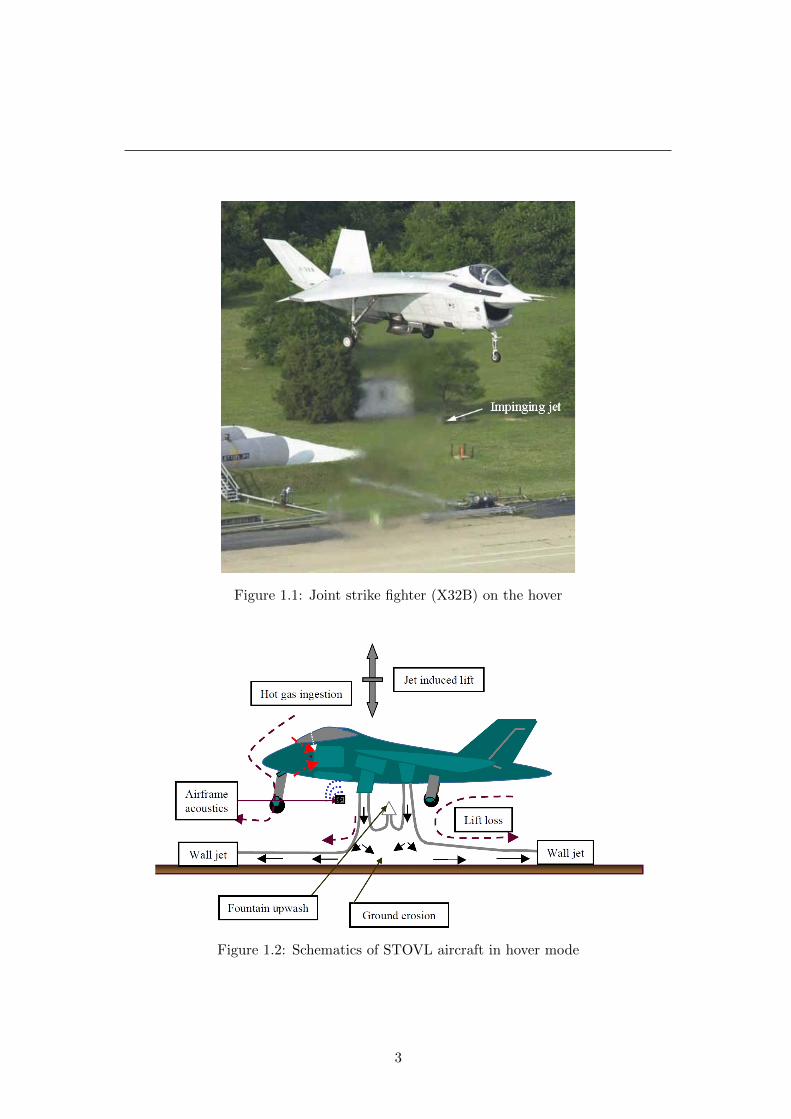
Figure 1.1: Joint strike fighter (X32B) on the hover
Figure 1.2: Schematics of STOVL aircraft in hover mode
3

1. INTRODUCTION
gas-turbine failure, and terrestrial rocket launch, and so on. Moreover, in some manu-
facturing industries free jets also require to impinge upon solid boundaries, such as in
laser cutting, surface cooling, materials removal, paint spraying, etc. Despite the sim-
ple geometry, the flow structure of supersonic impinging jet on a solid surface is rather
complex; it contains mixed supersonic and subsonic regions, and involves interaction of
shock and expansion waves with jet shear layers [Kim & Park, 2005; Lamont & Hunt,
1980]. Impinging jets are characterized by a strong coupling between the flow and
acoustic fields with a self-contained feedback mechanism that result in high amplitude
of sound tones. The feedback loop begins with the formation of turbulence structures
within the shear layer of the jet. These structures grow and convect downstream where
they interact with the impingement surface. Acoustic waves are created due to this
interaction and travel outside of the flow in the upstream direction. These acoustic
waves/perturbations eventually reach the receptivity location of the shear layer at the
nozzle exit where they excite the shear layer and lead to the formation of more struc-
tures, thus perpetuating the cycle. The initial formation of turbulence structures within
the shear layer is largely dependent on the frequency(ies) of forcing. The development
of structures is further influenced by the strong interaction between the flow and the
obstacle.
In supersonic impinging jets, the high speed and temperature lead to a severe me-
chanical and thermal loading on the impinging surface. It becomes oscillatory under
certain operating conditions after the initial transient impinging behavior. The un-
steady oscillation can make thermal and mechanical loading more severe. An oscilla-
tory supersonic impinging jet produces severe noise at discrete frequencies, which may
cause sonic fatigue of the structures and also may damage various instruments and
equipments. The unsteady oscillatory nature is caused by the feedback loop of the
downstream traveling vortical structures and the upstream propagating acoustic waves
Krothapalli [1985]; Powell [1988]; Tam & Ahuja [1990]. The energy of the feedback
loop is provided by the instability waves in the shear layer of the jet. Upon interacting
with the impinging surface, the downstream traveling coherent jet structures generate
strong pressure fluctuations near the impingement region that lead to acoustic waves
in the near sound field. The structure of impinging jet depends on the design Mach
number, that is, nozzle geometry, nozzle pressure ratio, the distance between nozzle
exit and obstacle and so on.
4
In the above mentioned examples, the dry air was considered as working gas. How-
ever, in most of the practical applications, as mentioned above, usually the working
gas is steam or moist air, which have not yet received the same level of attention in
supersonic jet technologies as single-phase gases. In these cases, the non-equilibrium
condensation Matsuo et al. [1985a]; Wegener & Mach [1958] may occur at the region
between nozzle exit and an object. In the supersonic flow with the condensation, the
surrounding gas will be heated by the release of latent heat of condensation. The
jet flow with non-equilibrium condensation may be quite different from that without
condensation. However, no considerable work has been done to study the effect of
non-equilibrium condensation on flow characteristics of supersonic impinging jets, so
far. Therefore, it requires to perform investigations to get a deep insight about the
effect of non-equilibrium condensation on the jet flow characteristics, wave and shock
structure of supersonic impinging jets. Although fundamental in nature, the research
in this numerical simulations is large part geared towards exploring the effects of non-
equilibrium homogeneous condensation on the self-induced flow oscillations, lift loss,
etc. of supersonic moist air impinging jets.
1.2 Background
1.2.1 Supersonic free jet
The propulsive force or thrust necessary for powered flight is provided by a jet through
nozzle. In case of STOVL aircraft axisymmetric convergent and convergent-divergent
(C-D) nozzles are used to produce this thrust. A convergent nozzle can at most reach
sonic conditions at the exit. In a C-D nozzle the wall contour on the inlet side converges
to a minimum area also known as the throat. After that it diverges from the throat
to the nozzle exit. The convergent portion of the nozzle accelerates the subsonic flow
to sonic conditions at the throat, then it is further accelerated to supersonic speeds in
the divergent region until it reaches the nozzle exit [Anderson, 1991]. The design Mach
number at the exit depends on the ratio of the nozzle exit area and the throat area.
Each C-D nozzle when operated at ideal conditions is designed for one Mach number.
Whether the nozzle operates at the ideal condition depends on the nozzle pressure ratio
of the flow. The nozzle pressure ratio (NPR) is defined as the stagnation pressure of
the jet divided by the ambient pressure. Design NPR is the pressure ratio at which the
5
1. INTRODUCTION
nozzle operates at the ideal, design condition. The critical NPR is the minimum NPR
necessary in order to achieve supersonic flow at the exit of the nozzle.
Ideally expanded jet
When the NPR is equal to the design pressure ratio for that particular nozzle, the
jet is said to be ideally expanded. A schematic of such a jet is shown in Fig. 1.3. In this
case the pressure at the nozzle exit is equal to the ambient pressure. In the majority of
the experiments performed in the current setup the jet was nominally ideally expanded.
Off-design jet
A C-D Nozzle can be operated at off-design conditions. When that is the case, two
different shock patterns in the core region are observed [Wishart, 1995]. First if the
nozzle pressure ratio is greater than the critical pressure but below the design pressure
ratio for that nozzle, the flow is considered overexpanded. Here, the exit pressure is
lower than the ambient pressure. In order to adjust to the ambient pressure the jet
flow has to go through a series of oblique shock waves. If the jet is highly overexpanded
then a normal shock also known as a Mach disc forms downstream of the nozzle [Garg,
2001]. A schematic of a highly overexpanded jet is shown in Fig. 1.4.
If the exit pressure is higher than the ambient pressure, meaning that the nozzle is
operated at a NPR higher than the design NPR, the jet flow becomes underexpanded.
In order for the exit pressure to equal to the back pressure (ambient pressure) the jet
flow is expanded through a centered expansion fan, as shown in Fig. 1.5. If the NPR
is further increased and the flow becomes highly underexpanded, the shock patterns in
the flow become even more complicated [Iyer, 1999].
Heated jet
Much work has been done in order to investigate the features of a cold or isothermal
supersonic jet. Isothermal or cold jets are jets where the stagnation temperature of the
jet (T0) is equal to the ambient temperature (Tamb). In those cases the temperature
ratio (TR), defined as stagnation temperature divided by ambient temperature, is equal
to one. However, most jets in aircrafts operate at very high stagnation temperatures
and therefore it is important to explore heated supersonic jets. Some research has been
done on the effect of temperature on supersonic free jets. Lau [1981] reported that the
6

Figure 1.3: Schematic of an ideally expanded jet
7

1. INTRODUCTION
spreading rate of the jet increases for supersonic jets when the temperature ratio of
the jet is increased above one. Additionally, he noticed a shortening of the potential
core of the jet when the jet was heated. Seiner et al. [1992] also report a shortening of
the potential core of the jet as well as an increase in mixing. They also find that there
is no significant change in the spreading rate of the shear layer when the temperature
of the jet is increased. There is however a significant decrease in jet half-width when
the temperature ratios are increased, up until about 10 jet diameters.This suddenly
changes at downstream locations when the jet half-width spreading starts increasing.
Most recently Wishart & Krothapalli [1994] reported some similar results. They
have found that with increased temperature ratio there is no significant effect on the
development of the jet shear layer but there is a significant increase of the mixing of the
jet in the downstream region. For jets at off-design conditions the temperature ratio
seems to have no effect on the structure of the shock cell pattern in the initial region
but they show that the decay of the centerline Mach number is enhanced. At the end
of the potential core there is a slight difference due to the shear layers merging sooner
for higher temperature jets.
The above results were obtained using free jets at different temperature ratios.
In order to be beneficial to the STOVL aircraft design, more research is needed to
determine how the temperature of the jet influences the characteristics of an impinging
jet. This is the focus of the present study.
1.2.2 Flowfield of impinging jet
Previous work has been done on isothermal, impinging, supersonic jets by Donaldson
& Snedeker [1971]; Donaldson et al. [1971], Lamont & Hunt [1980], Powell [1988], Tam
& Ahuja [1990], Messersmith [1995] and Alvi & Iyer [1999], among others. According
to the study of Donaldson & Snedeker [1971]; Donaldson et al. [1971] the flowfield
produced by a turbulent, axially symmetric jet, impinging perpendicular on a plate
can be described by three primary flow regimes (Fig. 1.6):
1. The Free Jet Region or Primary Jet Flow which is upstream of any strong local
effects of impingement and therefore shows the same characteristics as the before
described free jet flow [Iyer, 1999].
8
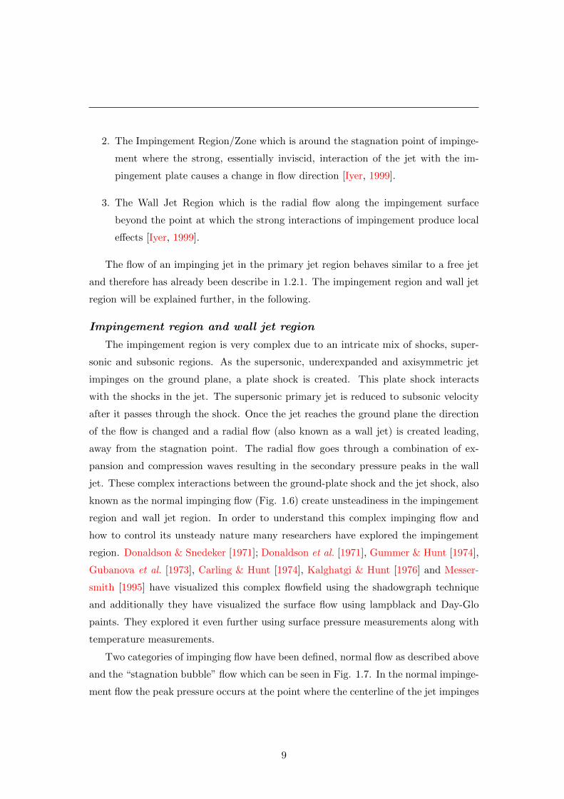
2. The Impingement Region/Zone which is around the stagnation point of impinge-
ment where the strong, essentially inviscid, interaction of the jet with the im-
pingement plate causes a change in flow direction [Iyer, 1999].
3. The Wall Jet Region which is the radial flow along the impingement surface
beyond the point at which the strong interactions of impingement produce local
effects [Iyer, 1999].
The flow of an impinging jet in the primary jet region behaves similar to a free jet
and therefore has already been describe in 1.2.1. The impingement region and wall jet
region will be explained further, in the following.
Impingement region and wall jet region
The impingement region is very complex due to an intricate mix of shocks, super-
sonic and subsonic regions. As the supersonic, underexpanded and axisymmetric jet
impinges on the ground plane, a plate shock is created. This plate shock interacts
with the shocks in the jet. The supersonic primary jet is reduced to subsonic velocity
after it passes through the shock. Once the jet reaches the ground plane the direction
of the flow is changed and a radial flow (also known as a wall jet) is created leading,
away from the stagnation point. The radial flow goes through a combination of ex-
pansion and compression waves resulting in the secondary pressure peaks in the wall
jet. These complex interactions between the ground-plate shock and the jet shock, also
known as the normal impinging flow (Fig. 1.6) create unsteadiness in the impingement
region and wall jet region. In order to understand this complex impinging flow and
how to control its unsteady nature many researchers have explored the impingement
region. Donaldson & Snedeker [1971]; Donaldson et al. [1971], Gummer & Hunt [1974],
Gubanova et al. [1973], Carling & Hunt [1974], Kalghatgi & Hunt [1976] and Messer-
smith [1995] have visualized this complex flowfield using the shadowgraph technique
and additionally they have visualized the surface flow using lampblack and Day-Glo
paints. They explored it even further using surface pressure measurements along with
temperature measurements.
Two categories of impinging flow have been defined, normal flow as described above
and the “stagnation bubble” flow which can be seen in Fig. 1.7. In the normal impinge-
ment flow the peak pressure occurs at the point where the centerline of the jet impinges
9

1. INTRODUCTION
on the ground as can be seen in the graph in Fig. 1.6. Why a stagnation bubble, also
known as a recirculation region is formed in the impingement zone at certain conditions
is a question that many studies have tried to explain. According to Gummer & Hunt
[1974], Gubanova et al. [1973], Ginzburg et al. [1973] and Kalghatgi & Hunt [1976],
the recirculating region is created due to the primary jet flow being separated from the
center of the ground plate surface by a thin layer of fluid. Due to this, the primary jet
impinges on the ground plane at a radial distance from the stagnation point leading to
maximum pressure at an annular location away from the ground plate center, as see in
the graph in Fig. 1.7.
This recirculating region results in enhanced convection, leading to lower temper-
atures as shown by Messersmith [1995]. Ginzburg et al. [1973] and Gubanova et al.
[1973] performed experiments using C-D nozzles with different divergence angles. Both
used surface pressure measurements, schlieren, pressure probe measurements to con-
firm the presence of reversible flow. They described the mechanism of creation of the
stagnation bubble as follows. When the jet shock and plate shock intersect a tail shock
is formed. This leads to a tangential discontinuity in velocity also known as the sli-
pline. This slipline divides the flow into two regions with the outer one having a higher
total pressure and higher velocity. While the slipline is not in contact with the imping-
ing plate, the mixing between the two regions occurs at the slipline. At certain plate
heights the slipline intersects with the ground plate and only some parts of the fluid
are drawn into the mixing zone and leave the central portion of the impingement zone.
The rest of the fluid, which is unable to overcome the pressure difference, accumulates
at the central point of the plate and forms a recirculating region also known as the
stagnation bubble. These studies have shown that the Mach number inside the stag-
nation bubble can reach 0.4 and the bubble diameter can be as large as 80% of the jet
diameter. Ginzburg et al. [1973] noted the absence of the stagnation bubble at very
small y/d. The oscillating nature of the flow causes the appearance and dispersion of
the recirculating region between two and three diameters. According to Ginzburg et al.
[1973], once y/d=3.4 is reached, the flow becomes more stable and the appearance of
the stagnation bubble is well defined at this height. Gubanova et al. [1973] observed
similar results but in their case the stagnation bubble presence is well pronounced at
y/d=3. Kalghatgi & Hunt [1976] conducted similar test with nozzles of varying Mach
numbers. They proposed that the bubbles are caused by the intersection of the plate
10
shock and the jet shock waves either right before crossing the jet centerline or right
after crossing the jet centerline. They implied that the bubble can also be a product
of some surface imperfection, like a scratch in the nozzle surface and therefore can be
easily eliminated by publishing the surface. Donaldson & Snedeker [1971]; Donaldson
et al. [1971] and Gummer & Hunt [1974] anticipated that the stagnation bubble in an
impinging jet is likely to be present when the impinging plate is stationed around the
position where the normal shock or a Mach disc are observed in a free jet.
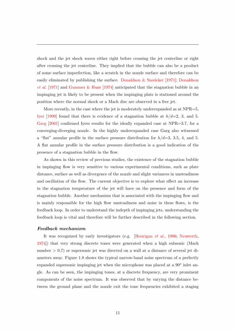
More recently, in the case where the jet is moderately underexpanded as at NPR=5,
Iyer [1999] found that there is evidence of a stagnation bubble at h/d=2, 3, and 5.
Garg [2001] confirmed Iyers results for the ideally expanded case at NPR=3.7, for a
converging-diverging nozzle. In the highly underexpanded case Garg also witnessed
a “flat” annular profile in the surface pressure distribution for h/d=3, 3.5, 4, and 5.
A flat annular profile in the surface pressure distribution is a good indication of the
presence of a stagnation bubble in the flow.
As shown in this review of previous studies, the existence of the stagnation bubble
in impinging flow is very sensitive to various experimental conditions, such as plate
distance, surface as well as divergence of the nozzle and slight variances in unsteadiness
and oscillation of the flow. The current objective is to explore what effect an increase
in the stagnation temperature of the jet will have on the presence and form of the
stagnation bubble. Another mechanism that is associated with the impinging flow and
is mainly responsible for the high flow unsteadiness and noise in these flows, is the
feedback loop. In order to understand the indepth of impinging jets, understanding the
feedback loop is vital and therefore will be further described in the following section.
Feedback mechanism
It was recognized by early investigators (e.g. [Hourigan et al., 1996; Neuwerth,
1974]) that very strong discrete tones were generated when a high subsonic (Mach
number > 0.7) or supersonic jet was directed on a wall at a distance of several jet di-
ameters away. Figure 1.8 shows the typical narrow-band noise spectrum of a perfectly
expanded supersonic impinging jet when the microphone was placed at a 90o inlet an-
gle. As can be seen, the impinging tones, at a discrete frequency, are very prominent
components of the noise spectrum. It was observed that by varying the distance be-
tween the ground plane and the nozzle exit the tone frequencies exhibited a staging
11
1. INTRODUCTION
phenomenon, which suggested that the tones were generated by a feedback loop.
The highly unsteady nature of supersonic impinging flow field can be explained
by a feedback mechanism (Fig. 1.9). The feedback loop is started with instability
waves that form in the shear layer of the jet near the nozzle exit. They grow as they
travel downstream and develop into large scale vertical structures. These structures can
be visible in flow visualization pictures like the shadowgraph technique [Alvi & Iyer,
1999]. As these structures travel downstream in the outer jet shear layer they entrain
the ambient air which leads to lift loss and mixing, as will be discussed further in the
following chapters. Once the large scale structures impinge on the ground plane they
generate acoustic waves which travel upstream in the ambient medium. These acoustic
waves in turn excite the shear layer near the nozzle exit resulting in the generation of
instability waves thus closing the feedback loop.
In the 1950’s Powell was the first one to describe the physics of the formation of
the feedback loop in free supersonic jets and additionally he provided a formula for
predicting the frequency of discrete tones (screech tones) generated by this mechanism.
Powells feedback formula is provided, as follows:
n± pfn
=
∫ h
0
dh
Ci+
h
Ca(1.1)
Here, h is the nozzle exit-to-plate distance, Ci is the convection velocity of the
downstream traveling large structures or Ci=0.5×Uj [Krothapalli et al., 1999], Ca is
the speed of the upstream traveling acoustic waves, n is arbitrary integer, n=1, 2, 3,
... ... (when n=1 corresponds to mode 1, n=2 corresponds to mode 2, etc.), and p is
the phase lag between the acoustic wave and convected disturbance.
These discrete tones are called impinging tones when the jet is impinging on a flat
plate. It was shown by Neuwerth [1974], Ho & Nosseir [1981], Powell [1988], Tam
& Ahuja [1990], Henderson & Powell [1993], and Krothapalli et al. [1999] that these
impinging tones are also generated by the feedback loop and therefore their frequency
can be predicted using Powells formula (Equation 1.1).
Due to the difficulty of measuring the convective velocity Ci of the downstream
traveling large scale structures most researchers assume the convective velocity to be
60 - 70% of the jet flow velocity when using Powells formula. Krothapalli et al. [1999]
12
obtained more accurate values for Ci using the PIV technique. They reported that the
convection velocity of the large scale structures for the free jet to be about 60% of the
mean jet exit velocity. For impinging jets, the convection velocity was about 50% of
the primary jet velocity and it increases with plate height. They also suggested that
for an impinging jet the convection velocity increases when the jet is underexpanded
or overexpanded due to the presence of a more pronounced shock cell structures.
Jet noise and unsteady loads
Some previous researchers (e.g. [Krothapalli et al., 1999]) reported that the presence
of the ground plane in an impinging jet significantly increases the OASPL and unsteady
loads on the nearby structure. At nearly ideally expanded conditions, Krothapalli et al.
[1999] found approximately an 8 dB increases relative to a free jet. The source of the
noise in the impinging jet has been a subject of inquiry for a long time. Most of the noise
of a subsonic impinging jet is generated in a region near the plate between one and three
diameters from the stagnation point Preisser [1979]. Otherhand, a comprehensive study
on the noise characteristics of an ideally and moderately under-expanded supersonic
impinging jet was conducted by Krothapalli et al. [1999]. They showed the acoustic
waves and demonstrated the origin of these waves somewhere within the impingement
region on the ground. For a moderately underexpanded jet, (design Mach number=1.5,
NPR=5), when the ground plane was closed to the nozzle exit, standoff shock or plate
shock was observed. In some cases, a local stagnation bubble was also observed in
the impingement region. The appearance and disappearance of the shock and the
associated separation or stagnation bubble may play an important role in determining
the local acoustic field. In their experiment, Krothapalli et al. [1999] also showed the
mode switching between helical and axisymmetric in the main jet column relative to
ground plane distance, which is similar at ideally and under-expanded conditions.
Lift loss
The loss of lift in STOVL aircraft while in hover mode has a critical impact on its
performance. A discussion of subsonic jets may be found in Margason et al. [1997];
however, little data are at present available for supersonic impinging jets in STOVL
configurations. For a supersonic impinging jet, Levin & Wardwell [1997] found a non-
monotonic lift loss as a function of jet NPR. Based on the flow visualization, they
speculated that this nonlinear lift loss behavior might be related to the jet shock cell
13
1. INTRODUCTION
structure. However, Krothapalli et al. [1999] found that shock cells play an insignificant
role in the lift loss except when the ground plane is in close proximity to the jet exit. In
their experiment to study the effect of lift loss, a circular lift plate, called “lift plate”,
was flush-mounted at the nozzle exit. From a summary of lift loss measurements for a
sonic nozzle, Krothapalli et al. [1999] further speculated that the nonlinear loss in lift,
at small ground plane distance, is somehow related to the appearance of the stand-off
shock and associated bubble. Furthermore, the high-speed wall jet is likely to play an
important role in determining the local pressure field and lift loss at very small lift-to-
ground plane distance. In their study, Krothapalli et al. [1999] also found that the lift
loss can be as high as 60% of the main jet thrust in the supersonic impinging jet when
the aircraft is very close to the ground. This significant lift loss would require a large
percentage of the propulsive power to overcome.
1.3 Literature review
Research on impinging jet normally on a flat plate has unfolded in a broad way. Some
researchers have concentrated on the hydrodynamics and investigated the lift loss, other
researchers focus on the produced sound tone and the aeroacoustic loading of the im-
pinging jets. Among them, earlier researchers investigated the flow structure and the
mean flow characteristics by using optical visualization techniques (schlieren, shadow-
graph, etc.) and mean surface pressure and temperature measurements. Henderson
[1966] conducted experimental investigation on supersonic impinging jets on flat plate.
He measured the pressure distribution on a flat plate for a variety of jet Mach num-
bers, plate incidence angles, and plate locations downstream of the nozzle outlet, and
used shadowgraphs to visualize the flowfield. He observed that for some operating
conditions the apparatus displayed an oscillatory instability which appeared to be a
Hartmann type. Chu et al. [1969] reported some theoretical results on jet impingement
and discuss certain points raised in the experimental study of Henderson [1966]. Don-
aldson and coworkers [Donaldson & Snedeker, 1971; Donaldson et al., 1971] conducted
experiments on subsonic and sonic air jets impinging on plates at various angles and
obtained surface pressure profiles of mean and turbulent properties. Carling & Hunt
[1974] made surface pressure and shadowgraph measurements of four different super-
sonic jets (Mach number varying between 1.64 and 2.77), impinging normally on a large
14
flat plate. Lamont & Hunt [1976, 1980] carried out experiments on the impingement
of under-expanded supersonic jets on plates and wedges. Shadowgraph pictures and
pressure measurements were used for the flow field analysis. Iwamoto [1990] reported
experimental study of under-expanded dry air sonic jets impinging on a flat plate. The
flow field was visualized using shadow photography and Mach-zehnder interferometry.
In consequence of the previous, Iwamoto et al. [1999] conducted experiment on the
impingement of supersonic jets on flat plate, using a convergent-divergent nozzle. The
flowfield at different under-expansion ratios and nozzle-plate distances was visualized
by schlieren photography. Recently, Ghanegaonkar et al. [2004] conducted experimental
investigation on the supersonic jet impingement. They conducted tests in a small-scale
rocket motor loaded with a typical nitramine propellant to produce a nozzle exit Mach
number of 3, and the jet was impinged on a plate aligned vertically to the nozzle axis.
Pressure transducers were used to measure the pressure rise due to jet impingement
on the plate, and tests were carried out to obtain the effects of nozzle divergence an-
gle, axial distance between the nozzle exit and the plate and the chamber stagnation
pressure on the flowfield. Nakai et al. [2006] experimentally investigated using pressure-
sensitive paints and Schlieren flow visualization the flowfields of jet impinging on an
inclined flat plate at various plate angles, nozzle-plate distances, and pressure ratios.
They eliminated the effect of temperature variation on the flat plate by the calibration
using temperature-sensitive paints. Comparing the results with the former experiment,
they clarified that the new efficient pressure/temperature-sensitive paint measurement
technique showing surface pressure map need much less effort compared to conventional
pressure tap measurement. At the same time, Ito et al. [2006] also experimentally in-
vestigated the flow fields of the supersonic jets impinging on an inclined flat plate at
high plate-angles using surface pressure measurement with pressure sensitive paint and
Schlieren flow visualization.
Some subsequent works have focused on the unsteady flow oscillations and acous-
tic properties specially on acoustic tones referred to as impingement tones, which are
caused by a feedback loop. For example, Alvi & Iyer [1999] studied the impinging jet
with lift plate, and noted the emergence of discrete peaks in the spectra of the un-
steady surface pressures, which match the impinging tone frequencies in the near-field
acoustic measurements. They suggests that these feedback loop-driven flow instabil-
ities are also responsible for the unsteady loads on the ground plane. In some cases
15
1. INTRODUCTION
these unsteady loads were measured to be as high as 190 dB, which coupled with
the high temperatures associated with lifting jets, can further aggravate the ground
erosion problem. Krothapalli et al. [1999] investigated the jets with both convergent
and convergent-divergent (C-D) nozzles, and the main findings of their work was the
intimate connection between the discrete impinging tones and the highly unsteady, os-
cillatory behavior of the impinging jet column. They demonstrated that, through the
generation of large-scale structures in the jet shear layer, the feedback phenomenon
might also be responsible for lift loss on surfaces in the vicinity of the nozzle. These
structures induce higher entrainment velocities that lead to lower surface pressures in
the jet vicinity and, consequently, a significant loss in lift. Thurow et al. [2002] used a
real-time imaging system to investigate the flow field of an ideally expanded impinging
rectangular jet, particularly explored the connection between the acoustic tones and
the development of large-scale structures within the mixing layer. Elavarasan et al.
[2000] investigated the characteristics of supersonic impinging jets using Particle Image
Velocimetry (PIV). The oscillations of the impinging jet generated due to a feedback
loop were captured in the PIV images. Consequently, an experimental investigation was
also performed by Lou et al. Lou et al. [2003] using Particle Image Velocimetry (PIV)
Technique of the flow and acoustic properties of an axisymmetric impinging jet, with
and without microjet control. The near-field acoustic measurements clearly showed
that the use of microjet control eliminates or significantly suppresses the impinging
tones, and reduces broadband spectral amplitudes. Crafton et al. [2006] investigated
the flow field associated with a jet impinging onto a surface at an inclined angle using
particle image velocimetry (PIV). The results indicated that as a free jet impinges on
a flat surface at an inclined angle the jet is turned by and spread laterally onto the
impingement surface. The impingement angle of the jet is the dominant parameter in
determining the rate of turning/spreading for the jet. The stagnation point was lo-
cated using the PIV data and was found upstream of the geometric impingement point
and upstream of the location of maximum pressure. The location of the stagnation
point is a strong function of impingement angle and a weak function of impingement
distance and pressure ratio. They compared the result of the location of the stagna-
tion point with the location of maximum pressure, and compared to a curve fit for the
location of maximum pressure based an exact solution of the NavierStokes equations
for a non-orthogonal stagnation flow.
16
Focusing on the unsteady flow properties of supersonic impinging jets, Powell [1988]
conducted some experimental observations and pointed out that the small instability
waves (vortices) around the jet shear layers and the consequent radial wall jet are
responsible for the noise as they interact with the flat plate and it produces sound
waves. Ho & Nosseir [1981] conducted extensive measurements of the near-field pres-
sure to explain the feedback mechanism, responsible for the sudden change observed
in the pressure fluctuations at the onset of resonance. The feedback loop begins with
the formation of turbulence structures within the shear layer of the jet. These struc-
tures grow and convect downstream where they interact with the impingement plate.
Acoustic waves are created due to this interaction and travel outside of the flow in the
upstream direction. These acoustic waves/perturbations eventually reach the receptiv-
ity location of the shear layer at the nozzle exit where they excite the shear layer and
lead to the formation of more structures, thus perpetuating the cycle. They found that
the frequencies produced could be predicted quite well by requiring that an integer
number of waves, N , exist in the feedback loop according to the equation:
N =fl
Uc+fl
a0(1.2)
where f is the frequency, l is the distance between the nozzle exit and the impingement
plate, Uc is the convective velocity of turbulence structures and a0 is the ambient
speed of sound. While Tam & Ahuja [1990] put forward another theoretical model for
the acoustic feedback loop, and clarified that the feedback is achieved by upstream-
propagating waves associated with the lowest-order intrinsic neutral wave modes of
the jet flow. In addition they also offered, for the first time, an explanation as to
why no stable impingement tones had been observed for (cold) subsonic jets with Mach
number less than 0.6. Furthermore, the new model allowed the prediction of the average
Strouhal number of impingement tones as a function of jet Mach number. Henderson
et al. [2002] performed experiments of sound producing impinging jets on small and
large plates, and the flow field was visualized using phase-locked shadowgraph and
phase-averaged digital particle image velocimetry (DPIV). The results suggested that
the Mach disk oscillates axially, a well defined recirculation zone is created in the
subsonic impingement region and moves toward the plate, and the compression and
expansion regions in the outer supersonic flow move downstream.
17
1. INTRODUCTION
Durox et al. [2002] reported that self-induced instabilities may arise when a pre-
mixed flame anchored on the rim of a burner impinges on a flat plate located in the
vicinity of the burner and facing the outlet. They carried out systematic experiments
on three burner sizes and three mean flow velocities provide the ranges of burner-to-
plate distances which induce an unstable oscillation. The flame motion was imaged and
the non-steady heat release, unsteady flow velocity at the burner outlet, and pressure
fluctuations in the burner and in the far-field were characterized. The flow velocity
is essentially sinusoidal while the heat release and far-field pressure feature a strong
harmonic content. It was shown that the burner acts like a Helmholtz resonator but
the fundamental oscillation frequency evolves around the resonator frequency as the
burner-to-plate separation was changed. The sudden reduction of flame area produced
by the perturbed flame impinging on the plate produces an intense source of sound
which drives the system. They presented a model described the dynamics of the sys-
tem and the predicted signal relationships and fundamental frequency of oscillation,
and their experiments revealed that interactions between perturbed flames and solid
boundaries could play an important role in the development of combustion instabilities.
Beyond the aerodynamic fields, some researches also have been conducted on other
engineering fields, such as Shukla et al. [2000] put forward their step with a view to-
ward developing the next generation of coatings using nanopowders, a cold gas dynamic
spray (CGDS) technique in which a powder feeder is used to inject nanopowder ag-
glomerates into a supersonic rectangular jet. The powder particles gain speeds of up
to 700 m/s through momentum transfer from the jet and bond to the substrate surface
due to kinetic energy dissipation. The benefit of this process is that the material does
not undergo any chemical changes during coating formation. To improve the quality of
the coatings produced, the flapping motions produced by supersonic jet impingement
were studied. They quantified powder particle velocities and the jet impingement flow
field using particle image velocimetry (PIV). Subsequently, Karimi et al. [2006] made a
CFD model for the cold gas dynamic spray process. They simulated the gas dynamic
flow field and particle trajectories within an oval-shaped supersonic nozzle as well as
in the immediate surroundings of the nozzle exit, before and after the impact with the
target plane. Chen et al. [2000] conducted both numerical and experimental works on
the interaction of a supersonic, turbulent axisymmetric jet with the workpiece in laser
machining. Numerical simulations were carried out using an explicit, coupled solution
18
algorithm with solution-based mesh adaptation. Their model was able to make quanti-
tative predictions of the pressure, mass flow rate as well as shear force at the machining
front. Effect of gas pressure and nozzle standoff distance on structure of the supersonic
shock pattern was studied. Other hand, experiments were carried out to study the
effect of processing parameters such as gas pressure and standoff distance. They have
reported that the interaction of the oblique incident shock with the normal standoff
shock contributes to a large reduction in the total pressure at the machining front and
when the nozzle pressure is increased beyond a certain point. The associated reduction
in flow rate, fluctuations of pressure gradient and shear force at the machining front
could lower the material removal capability of the gas jet and possibly result in a poorer
surface finish. The laser cutting experiments show that the variation of cut quality are
affected by shock structures and can be represented by the mass flow rate. Liu &
Kendall [2004] numerically simulated the gas dynamics and temperature distribution
of a transient impinging jet, typically used to deliver powdered drug or vaccines ballis-
tically to the skin. They performed their calculations with the unsteady compressible
Navier-Stokes equations, solved using a modified implicit flux vector splitting (MIFVS)
difference scheme with a modified k − ε model. Firstly, calculated pressure histories
were compared with corresponding measurements in an unsilenced biolistic device, with
good agreement. Secondly, they extended the calculation to a silenced geometry, with
an emphasis on the gas properties immediately above a skin target. A peak stagna-
tion gas temperature of 420C was revealed within 175µs of diaphragm rupture. The
temperature of the following driver helium gas suddenly drops to below - 100C before
approaching ambient temperature within 1 ms. The effect of this impinging jet on the
human skin was subsequently explored by a one-dimensional convection heat transfer
model. On the skin surface, a peak fluctuation of [+5.5C, - 4.5C] was recorded during
the operation process. Beyond the outer skin layer, called the stratum corneum (i.e.
> 10.6µ), temperature deviations from the normal condition are trivial. Therefore, the
heat transfer between the biolistic jet and skin is negligible. Their predicted result was
consistent with pain-free clinical trial observations.
Numerical simulations of impinging jets have also been carried out. Among them,
Belov et al. [1973] made approximate solution of the problem on an axisymmetrical un-
derexpanded supersonic jet impinging upon a normal flat plate within the initial length
of the jet. The results of the calculation obtained in the ideal liquid treatment showed
19

1. INTRODUCTION
that there exists appreciable vorticity in a subsonic region close to the plate. They also
made calculation of a viscous flow and heat transfer in the vicinity of the stagnation
point. Kashimura et al. [1998] and Kim et al. [2002] investigated the characteristics
and mechanism of the self-induced oscillation of Mach disk during the impingement on
a cylindrical body using both the flow visualization and numerical calculation. The
instabilities in a supersonic impinging jet are investigated numerically and as well as
experimentally by Hourigan et al. [1994, 1996]. They found that the frequency and na-
ture of the dominant instabilities is a function of the impingement distance, and there
are two modes of instability. Flow behavior of under-expanded coaxial impinging jets
was investigated both experimentally and numerically by Masuda & Moriyama [1994].
They fabricated and tested two converging coaxial nozzles, one with outer annular jet
parallel to an inner circular one, and the other with inclined annular jet. The flow visu-
alization, pressure measurements and numerical results explained that the presence of
the outer annular jet has significant effects on reducing the Mach disk diameter which
formed in the inner jet. Kim & Chang [1994] numerically investigated the flow struc-
ture of an underexpanded supersonic jet with high reservoir temperature impinging on
a flat plate with TVD scheme. They found that when the temperature of the flow
field is high enough to cause chemical reaction, the specific heat ratio γ is no longer
equal to 1.4, nor constant. They considered the equilibrium flow assuming the effect
of high temperature gas on the impinging jet by using specific heat ratio and speed of
sound given by correlation polynomials of thermodynamic variables. Gorshkov & Uskov
[2002] studied, both experimentally and theoretically, the influence of geometric and
gas-dynamic parameters on the flow structure and parameters of self-sustained oscilla-
tions in supersonic overexpanded jets interacting with a normally located plane finite
obstacle. They found that the geometric Mach number and the half-angle of nozzle
expansion exert a significant effect on the interaction process. A numerical analysis on
the modes of oscillation that arise when under-expanded supersonic jets hit an obstacle
was done by Roslyakov & Sadkov [2000]. Large Eddy Simulation methodology to the
simulation of impinging jet flow fields are presented by Arunajatesan & Sinha [2002].
Loh [2005] numerically studied the near-field noise of an under-expanded supersonic jet
from a converging nozzle impinging normally on a flat plate. Recently, Kim & Park
[2005] used the popular TVD upwind scheme in simulating the supersonic impinging
jets. They focused on the oscillatory flow features associated with the variation of
20
the nozzle-to-plate distance and nozzle pressure ratio, analyzed the frequencies of the
surface pressure oscillation and flow structural changes. Sakakibara & Iwamoto [2002]
also used TVD scheme to study oscillations in impinging jets and the generation of
acoustic waves and found that the flow oscillated when the nozzle-to-plate distance
was greater than 2.3 times the exit diameter of the convergent nozzle, and also showed
that the frequency of the surface pressure oscillation exhibited staging behavior. Wu
et al. [2002] made a comprehensive numerical study of jet flow impingement over flat
plates, and they solved 3D N-S equations and their computational domain included
the convergent-divergent nozzle and the external field. McIlroy & Fuji [2007] compu-
tationally simulated the supersonic under-expanded jets impinging on a inclined flat
plate. For simulations, plate angle, distance between the nozzle exit and the plate,
and the PR (pressure ratio) were parametrically changed. Their results showed that
there are four mechanisms leading to the localized pressure peaks on the plate surface:
(1) stagnation of the main jet flows, (2) normal shock wave in the upstream area, (3)
reattachment of the separated flows over the plate surface, (4) interaction between the
intermediate tail shock and the plate surface boundary layer. Moreover, the investiga-
tion of intensities of the pressure peaks showed that the pressure peak (1) caused by
the stagnation of the main jet flows is almost independent from PRs, but the pressure
peak (2), (3), (4) become higher at lower PRs. This happens due to the existence of
a jet shock intercepting the flow outside and the ambient pressure does not affect to
the total pressure of the main jet flows. Yaga et al. [2006] conducted 3D investigations
on the flow characteristics of rectangular under-expanded impinging jets both experi-
mentally and numerically. Jun et al. [2008] numerically studied the interaction of a gas
jet with a workpiece in laser machining by investigating the influence of the processing
parameters on the dynamic characteristic of the gas flow.
Considerable research studies were carried out to examine jet impingement and heat
transfer rates from the impingement surface. Hrycak [1981] made a detailed literature
review on the heat transfer from impinging jets. They reviewed the available litera-
ture on the subject of flow patterns and heat transfer resulting from impinging jets,
and clarified that despite some accomplishments, there still exists necessity for both
analytical and experimental work, before the heat transfer aspects of the impinging
jets are properly understood. Confined impinging and opposing jets are studied by
Hosseinalipour & Mujumdar [1995]. They indicated that the predictions of impinging
21

1. INTRODUCTION
jets agree with the experimental results when the turbulence model was selected prop-
erly. Jet impingement and heat transfer were considered by Herwig et al. [2004]. They
indicated that the instability created in the jet through the vortex shedding improved
the heat transfer as compared to a steady impinging jet. Seyed-Yagoobi [1996] studied
the heat transfer characteristics of the jet impingement emanating from different types
of nozzles. He indicated that self-oscillating jet impinging nozzle provided improved
heat transfer performance when the nozzle-to-plate spacing was less than the optimal
spacing for the plain jet emerging from the nozzle. Amano & Brandt [1984] investi-
gated the flow structure due to jet impingement onto a flat plate and flowing into an
axisymmetric cavity. They showed that the near-wall models for the kinetic energy
and turbulent shear stress gave good predictions of the skin friction coefficients. The
effects of nozzle diameter on heat transfer and flow structure due to impinging jet were
examined by Lee & Lee [2000]. They showed that the local Nusselt number increased
with increasing nozzle diameter in the stagnation region while keeping the other flow
parameters constant, which was attributed to an increase in the jet momentum and
turbulence intensity level with the large nozzle diameter. Heat transfer due to jet im-
pingement onto a flat plate and influence of nozzle-plate spacing on the heat transfer
rates were examined by Lytle & Webb [1994]. They indicated that the accelerating
fluid between the nozzle and the plate gap as well as an increase in the local turbulence
resulted in substantially increase in the local heat transfer rates from the plate surface.
Ramezanpour et al. [2007] conducted a numerical study to investigate heat transfer in
turbulent, unconfined, submerged, and inclined impinging jet discharged from a slot
nozzle. They clarified that in inclined impinging jet by movement of stagnation point
to the uphill side of the impinging plate, the location of the maximum Nusselt number
moves to the uphill side of the plate. However, the movement increases by increasing
of H/D and by decreasing of Reynolds number and inclination angle. In addition,
the flow streamlines were consistent with location of the heat transfer peak on the im-
pinging surface. Most recently, Shuja et al. [2009] conducted numerical investigation
on the jet impingement onto a conical cavity. They considered annular nozzle and
jet impingement onto a conical cavity, and examined the heat transfer rates from the
cavity surfaces for various jet velocities, two outer angles of the annular nozzle, and
two cavity depths. Here, it is mentioned that the most above mentioned studies on jet
22
impingements onto cavity and heat transfer have only been concerned with subsonic
flow.
1.4 Objectives
As stated earlier, no considerable work has been done to study the effect of non-
equilibrium homogeneous condensation on the flow characteristics of supersonic im-
pinging jets, so far. The focus of the present numerical study is to investigate the effect
of non-equilibrium homogeneous condensation on the flow characteristics particularly
on the self-induced oscillations in the flowfield of supersonic impinging jets under differ-
ent operating conditions. In order to validate the present numerical code, firstly, both
experiments and numerical investigations have been conducted on the supersonic moist
air jets at different nozzle pressure ratios. The predicted results of supersonic moist air
jets were compared with the present experimental data as well as with the experimen-
tal results of Addy [1981]. Experiments have also been conducted on the supersonic
impinging jets under different operating conditions, and the results were compares with
the numerically predicted data to further verify the validity of computational results.
Again, very few researches have been conducted only on the impinging jets onto
the cylindrical cavity, so far, and most studies have only been concerned with subsonic
flow. However, the study on the supersonic impinging jets onto the cylindrical cavity
has not yet been performed, so far. Therefore, another objective of the present study
is to numerically investigate the flow characteristics of supersonic impinging jets onto
cylindrical cavity, and the effect of non-equilibrium homogeneous condensation on their
flow characteristics. Thus, the objectives of the present study can be summarized as
follows:
1. to study numerically the effect of non-equilibrium homogeneous condensation
on flow characteristics especially on the jet flow structure and acoustic waves
of supersonic impinging moist air jets on a flat plate at different nozzle pressure
ratios with varying nozzle-to-plate distances and initial degree of supersaturation.
2. to conduct numerical and experimental studies on the supersonic moist air jets
in order to verify the validity of using the present numerical code.
23

1. INTRODUCTION
3. to conduct experiments on the supersonic impinging jets on a flat plate to further
verify the validity of the present computational results.
4. to numerically simulate the supersonic impinging jets onto the cylindrical cavity,
and to investigate the effect of non-equilibrium homogeneous condensation on
their flow characteristics.
1.5 Outline of the dissertation
The motivation and a survey of the literature associated with the research depicted in
this dissertation are presented in Chapter 1. The physics of supersonic free jet flows,
their impingement on a solid surface and flowfields, feedback mechanism, acoustic wave,
and lift loss are also described in Chapter 1.
Condensation phenomena, and the related theories associated with homogeneous
nucleation and droplet growth, etc. that were used for simulating the liquid-phase
produced from the non-equilibrium homogeneous condensation in the flowfield of su-
personic impinging moist air jets are described in Chapter 2.
In Chapter 3, a detailed description about the governing equations and their trans-
formation to generalized curvilinear coordinate, turbulence model used in the study are
presented.
Numerical methods used in this research are described in Chapter 4, which contains
a description of the numerical scheme employed, convergence criteria of the scheme and
also a description of the conditions used for numerical simulation. Chapter 5 presents
the experimental setup and procedure.
The numerically predicted results of supersonic moist air jets that are compared
with the experimental data in order to verify the validity of the present numerical code
are presented in Chapter 6. A comparison between the present predicted results and
experimental results of Addy [1981] is also presented in this chapter. Experimental
investigation on supersonic impinging jets on a flat plate that also conducted in order
to verify the validity of the code developed for the present numerical simulations is
depicted in Chapter 7. Numerical results of supersonic impinging moist air jets on a
flat plate at different nozzle pressure ratios and initial degree of supersaturation with
varying nozzle-to-plate distances are also presented in Chapter 7. The predicted results
24
of the effect of non-equilibrium condensation on the jet flow structure, shock structure,
self-induced flowfield oscillation, etc. are also described in this chapter.
Chapter 8 presents numerical results of supersonic impinging jets onto cylindrical
cavity, and also showing results of the effect of non-equilibrium condensation on their
flow characteristics.
Chapter 9 presents the conclusions of this thesis, and recommendations for future
work. The thermophysical properties and the relational expressions of some thermo-
physical properties are given in Appendix A. This is followed by bibliography.
25

1. INTRODUCTION
Figure 1.4: Schematic of an overexpanded jet
26

Figure 1.5: Schematic of an underexpanded jet
27
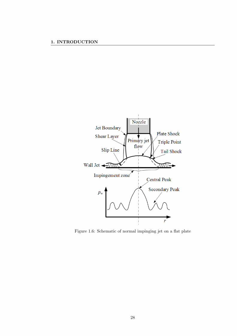
1. INTRODUCTION
Figure 1.6: Schematic of normal impinging jet on a flat plate
28

Figure 1.7: Schematic of a impinging jet flow with stagnation bubble
Figure 1.8: The near-field narrowband frequency spectra of an ideally expanded freeand impinging jet. (NPR=3.7, h/d=4) [Krothapalli et al., 1999]
29
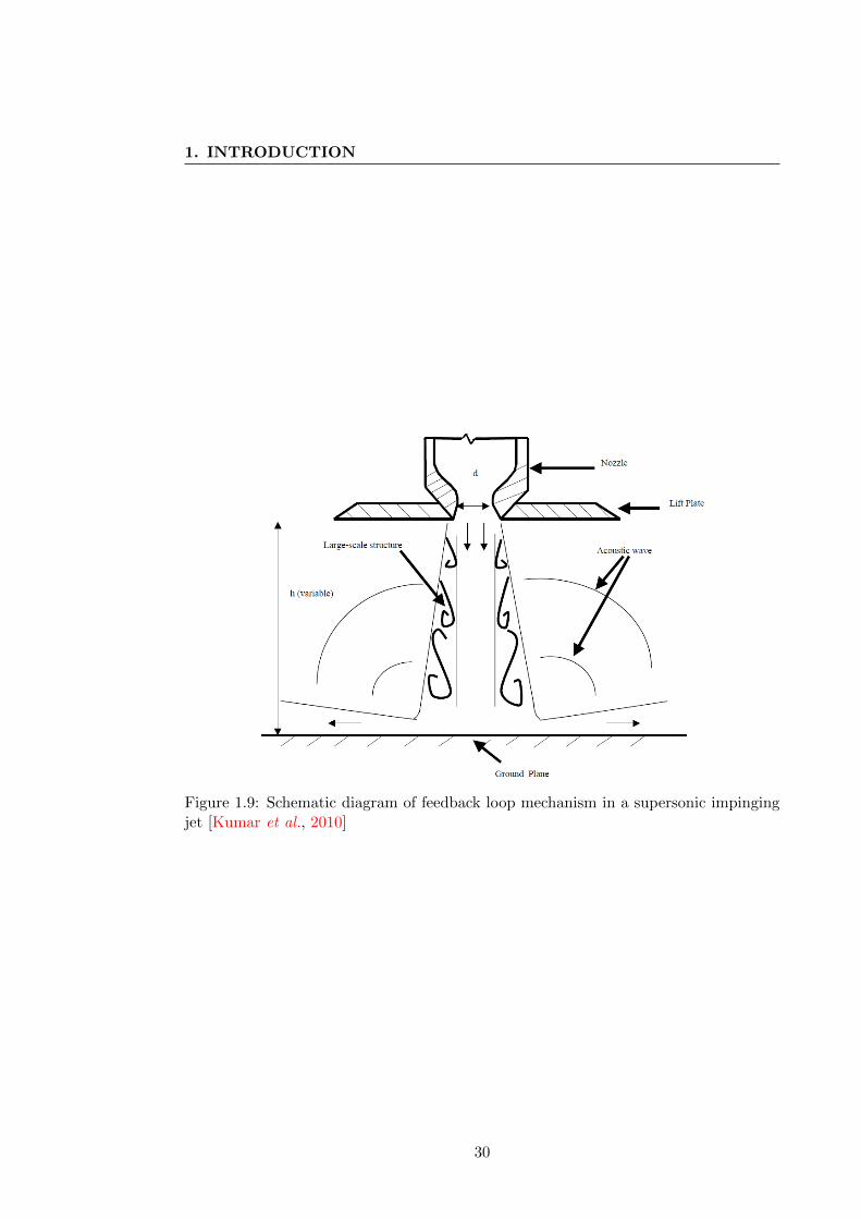
1. INTRODUCTION
Figure 1.9: Schematic diagram of feedback loop mechanism in a supersonic impingingjet [Kumar et al., 2010]
30
Chapter 2
Condensation phenomena
2.1 Introduction
Most human beings recognize the effects of gravity and condensation as phenomena
happening everywhere around in nature. Formation of tiny droplets on every flower or
leaf is a routine spectacle in every early morning all around the planet. ‘Breath figures’
or dew formation on windows or spectacles [Beysens et al., 1991], transformation of
clouds into rain, condensation of water in cloud chamber [Courtney, 1968], microemul-
sions and macroemulsions stability [Fletcher & Horsup, 1992], creaming of emulsions
[Bibette et al., 1992], grain growth [Wrner et al., 1991], etc., are problems of consid-
erable interest and pose important questions to be understood in condensed-matter
physics. In thermodynamics language this phenomena is known as a first-order phase
transition. Heterogenous and homogenous [Chernov, 1984] are the names for the two
ways of a saturated vapor condensation. When vapor condenses on an inhomogeneous
solid surface or a seed or a fast particle (Wilson chamber), the process is named het-
erogeneous condensation. But when a pure saturated vapor is condensed by density
fluctuations, the condensation is called homogenous. From the thermodynamic point
of view [Abraham, 1974], heterogeneous and homogeneous differ on the density value at
which each fit occurs. To trigger condensation, the later process requires higher-density
values than the former.
Phase transition is also encountered in high speed aerodynamics (transonic or su-
personic flows). In supersonic flows where water vapor contained in the main flow,
rapid expansion may give rise to homogeneous non-equilibrium condensation [Bakhtar
31
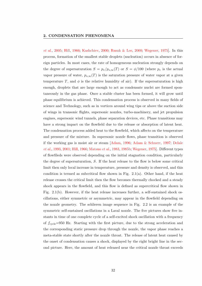
2. CONDENSATION PHENOMENA
et al., 2005; Hill, 1966; Kashchiev, 2000; Rusak & Lee, 2000; Wegener, 1975]. In this
process, formation of the smallest stable droplets (nucleation) occurs in absence of for-
eign particles. In most cases, the rate of homogeneous nucleation strongly depends on
the degree of supersaturation S = pv/ps,∞(T ) or S = φ/100 (where pv is the actual
vapor pressure of water, ps,∞(T ) is the saturation pressure of water vapor at a given
temperature T , and φ is the relative humidity of air). If the supersaturation is high
enough, droplets that are large enough to act as condensate nuclei are formed spon-
taneously in the gas phase. Once a stable cluster has been formed, it will grow until
phase equilibrium is achieved. This condensation process is observed in many fields of
science and Technology, such as in vortices around wing tips or above the suction side
of wings in transonic flights, supersonic nozzles, turbo-machinery, and jet propulsion
engines, supersonic wind tunnels, phase separation devices, etc. Phase transitions may
have a strong impact on the flowfield due to the release or absorption of latent heat.
The condensation process added heat to the flowfield, which affects on the temperature
and pressure of the mixture. In supersonic nozzle flows, phase transition is observed
if the working gas is moist air or steam [Adam, 1996; Adam & Schnerr, 1997; Delale
et al., 1993, 2001; Hill, 1966; Matsuo et al., 1983, 1985b; Wegener, 1975]. Different types
of flowfileds were observed depending on the initial stagnation condition, particularly
the degree of supersaturation, S. If the heat release to the flow is below some critical
limit then only local increase in temperature, pressure and density is observed, and this
condition is termed as subcritical flow shown in Fig. 2.1(a). Other hand, if the heat
release crosses the critical limit then the flow becomes thermally chocked and a steady
shock appears in the flowfield, and this flow is defined as supercritical flow shown in
Fig. 2.1(b). However, if the heat release increases further, a self-sustained shock os-
cillations, either symmetric or asymmetric, may appear in the flowfield depending on
the nozzle geometry. The schlieren image sequence in Fig. 2.2 is an example of the
symmetric self-sustained oscillations in a Laval nozzle. The five pictures show five in-
stants in time of one complete cycle of a self-excited shock oscillation with a frequency
of fcycle=950 Hz. Starting with the first picture, due to the strong acceleration and
the corresponding static pressure drop through the nozzle, the vapor phase reaches a
meta-stable state shortly after the nozzle throat. The release of latent heat caused by
the onset of condensation causes a shock, displayed by the right bright line in the sec-
ond picture. Here, the amount of heat released near the critical nozzle throat exceeds
32
the possible amount of heat for a steady solution. Hence, the shock can not find a
stable position and propagates upstream, even trough the nozzle throat (pictures 2-4).
Thereby, the shock raises the temperature and the vapour phase behind the shock is
no longer subcooled. Thus, re-offset of the condensation process, the flow again accel-
erates to a velocity where the vapour phase reaches a meta-stable state and the next
cycle starts (picture 1). Further increase of φ0 will finally provoke physical instabilities
and make the oscillation unsymmetric. Example of such an asymmetric flow structure
is shown in Fig. 2.3. Moreover, structural fatigue and performance degradation in
steam turbine plat can be seen due to the condensation of steam at the last stage of
LP turbine [White & Young, 1993].
Beyond these aerodynamic fields, condensation plays a significant role in other
engineering applications. In a gas phase chemical reactor, the undesired formation
of liquid droplets might severely reduce the reaction rate. The nucleation process is
deliberately induced to accomplish separation of toxic gases in gas purification plants.
Condensation may be important in free jets in EUV (Extreme Ultra-violet) lithography
[de Bruijn et al., 2003], a new way of printing circuit patterns onto silicon. In this
relatively new application, the jet is formed by xenon flowing from a reservoir through
a nozzle into a lower pressure environment such that xenon is expanding rapidly and
condensation takes place. The mixture of vapor and droplets will form a plasma by
heating it using a laser. Once the plasma is created, electrons are generated and light
is radiated at 13 nm (EUV light).
2.2 Condensation & nucleation
The phenomenon of condensation and nucleation are of fundamental importance in
many fields such as atmospheric physics, astrophysics, aeronautical sciences, nuclear-
reactor technology, material sciences, etc. They must be considered in weather pre-
diction, aerosol formation, metallurgical techniques, high-speed wind tunnel design,
steam-turbine nozzle design, rocket performance and high-intensity molecular beams,
etc. The processes include condensation of supersaturated vapor with or without foreign
nuclei, crystal formation from vapor, melted and solid-liquid solutions, phase changes
in solid states, crack nucleation in solids, and crystallization of polymers.
33

2. CONDENSATION PHENOMENA
(a) Subcritical flow
(b) Supercritical flow
Figure 2.1: Schlieren pictures of steady flow experiments in a supersonic nozzle S2[Adam, 1996]
34

Figure 2.2: Schlieren visualization of self excited shock oscillation in a Laval nozzle[Wendenburg, 2009]
35

2. CONDENSATION PHENOMENA
In the earliest stage, the first description on condensation phenomena of steam
started from Helmholtz in 1887. An experiment on condensing flow of supersatu-
rated steam in the steam turbine was conducted by Stodola in 1920, and that was the
first attempt to describe the condensation phenomenon from engineering point of view
[Stodola, 1927]. In 1940’s, condensation in supersonic flow field became a very impor-
tant research area, and a lot of full scale experimental and analytical researches were
done on condensation in the industrial supersonic wind tunnels, nozzles, steam turbine
expansions, etc. [Hill, 1966; Oswatitsch, 1942; Pouring, 1965; Wegener, 1954; Wegener
& Mach, 1958; Wegener & Pouring, 1964]. The theory of condensation phenomenon in
a chemically and physically pure gaseous medium, i.e., the theory of homogeneous nu-
cleation, has been developed by Volmer and Weber, Farkas, Becker and Doring, Frenkel,
and Zeldovich. After that, several authors have tried to improve this classical theory
bases on a semi-phenomenological model, by treating homogenous nucleation from a
statistical mechanical viewpoint. Parallel to this work, extensive experimental and an-
alytical investigations of water-vapor condensation of air primarily in steady supersonic
nozzle flows were carried on, both to check the validity of various available nucleation
theories and to solve Gasdynamics problems with condensation of interest in different
areas of engineering. Moreover, Volmer [1945] and Frenkel [1946] did some of typical
researches on the condensation nuclei generation rate. Abraham [1971a,b] worked on
the movement of the minute cluster using thermodynamic approach, and did some re-
searches theoretically on the generation process of condensate nuclei. Afterwards, the
study of condensation element has been extended from steam to N2 and kept spread-
ing to the polyatomic vapors of CO2 and CO2, C6H6, CHCL3, CCl3F, and C2H5OH
[Dorfeld & Hudson, 1973; Katz, 1970]. Sislian [1975] made a detailed analytical and
numerical study of homogeneous nucleation and condensation of water vapor with or
without a carrier gas in the non-stationary rarefaction wave generated in a shock tube
and predicted the effects of condensation on the flow variables.
Nucleation and condensation in compressible flows are of importance in the aerospace
science in designing supersonic and hypersonic wind tunnels, rocket nozzles, etc. In
turn, such flows provide fundamental data needed for an understanding of nucleation
and condensation processes. The heat release due to condensation can be a signifi-
cant flow disturbance. Details of condensing flow field structures were clarified, firstly,
through some experimental studies on condensation of the moist air in Laval nozzle by
36
Wegener & Pouring [1964] and Pouring [1965]. In this respect, well established flows in
supersonic nozzles and shock tubes have provided useful data in understanding macro-
scopic processes of nucleation and condensation. Reviews of such investigations were
made by Wegener [1954, 1969, 1975].
2.2.1 Condensation shock wave: a historical review
Now-a-days most researchers give emphasis on the basic problems of transonic and su-
personic flows. On of the important and at first mystifying phenomena that emerged
from experimental investigations in supersonic wind tunnels was the condensation
shock. Later such shock were noticed in the flow over an airfoil in experiments by
Liepmann in 1941.
Many investigators have been studied on the supersaturation phenomena in air and
water vapor mixtures for a considerable length of time. In fact, the subject was rather
remote form its line of thought so that the first appearance of effects of supersatura-
tion were somewhat mysterious and inexplicable. With the advent of the supersonic
wind tunnel, trouble was encountered in producing good flow conditions because of
the appearance compression shocks system downstream of the throat. Such shocks
were found to vary in location, appearance and strength from day to day. As at first
thought, this phenomenon could not be the result of imperfections in the contours of
the walls and was first discussed by Prandtl in 1935 at the Volta High Speed Conference
but no satisfactory explanation for it was advanced at that time. Wieselsberger had
also noted such shocks in his high speed wind tunnel experiments and because of their
characteristic appearance he had termed them ‘X-shocks’. He suspected correctly that
their appearance was associated with the humidity of the air. In the year of 1942, by
a series of experiments of Hermann in collaboration with Wieselsberger, it was varified
this suspicion and clarified that the so-called ‘X-shocks’ were the result of a sudden
condensation of water vapor in the air stream [Wegener, 1975]. In theoretical analy-
sis, at first, the thermodynamic concept was introduced by Heybey in the supersonic
condensing flow of moist air [Wegener & Mach, 1958].
The oscillating phenomenon of shock due to the non-equilibrium condensation was
discovered by Schmidt [1962]. After that, a lot of experimental researches were per-
formed using supersonic wind tunnels and Ludwieg tube [Matsuo et al., 1983, 1985b;
37
2. CONDENSATION PHENOMENA
Wegener & Cagliostro, 1973; Zierep & Lin, 1967]. A theoretical research was con-
ducted by Barschdorff to calculate the approximate frequency [Barschdorff & Fillipov,
1970], and in 1975 the first numerical analysis of one-dimensional primitive equations
using finite difference method was done by Saltanov & Tkalenko [1975]. They observed
that the condensation shock, due to the non-equilibrium homogeneous condensation
was generated in the divergent part of the Laval nozzle, oscillated the flowfield and re-
ported that there were two forms of shock oscillation in the divergent area of the nozzle.
The first form, spread to the upstream of the throat and disappeared, while the second
form repeated generation, propagation, disappearance. Meanwhile, the two-dimension
calculation was done by White and Young in 1993, and they found big change in shock
oscillation patterns [White & Young, 1993]. It was reported that there was not only two
forms but also included three forms of oscillations, and the third form of oscillation of
condensation shock that oscillated the flow field without disappearing in the divergent
area of the nozzle, by Adam & Schnerr [1997].
In recent years, a great variety of numerical simulation techniques have been de-
veloped with the rapid development of the computer, and the numerical simulation
techniques have become the most powerful tools to clarify the more complex, more
interesting condensation phenomena. Many researches have been done on the con-
densation shock [Kawada & Mori, 1973; Matsuo et al., 1984a, 1985a, 1986] and espe-
cially on the condensation phenomena in a supersonic nozzle [Schnerr, 1986; Schnerr &
Dohrmann, 1990; Young, 1992; Zierep, 1990].
2.2.2 Condensation in a supersonic nozzle
Condensation and nucleation in nozzle flows are important in connection with the
performance of supersonic and hypersonic wind tunnels, rocket nozzles, steam turbines,
and cooling towers, etc. Extensive theoretical and experimental studies have been
reported since Stodola in 1927. The qualitative effects of condensation in nozzle flows
are quite well known and have been described in details by Wegener & Mach [1958]
in a comprehensive review paper. Recently, the supersonic nozzle-flow technique was
applied successfully to studies of homogeneous-nucleation and condensation problems.
Most vapors have a wide range of stagnation states from which an expansion isen-
trope will intersect the vapor-liquid coexistence line, as shown in Fig. 2.4. When a
38
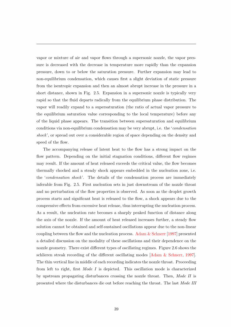
vapor or mixture of air and vapor flows through a supersonic nozzle, the vapor pres-
sure is decreased with the decrease in temperature more rapidly than the expansion
pressure, down to or below the saturation pressure. Further expansion may lead to
non-equilibrium condensation, which causes first a slight deviation of static pressure
from the isentropic expansion and then an almost abrupt increase in the pressure in a
short distance, shown in Fig. 2.5. Expansion in a supersonic nozzle is typically very
rapid so that the fluid departs radically from the equilibrium phase distribution. The
vapor will readily expand to a supersaturation (the ratio of actual vapor pressure to
the equilibrium saturation value corresponding to the local temperature) before any
of the liquid phase appears. The transition between supersaturation and equilibrium
conditions via non-equilibrium condensation may be very abrupt, i.e. the ‘condensation
shock ’, or spread out over a considerable region of space depending on the density and
speed of the flow.
The accompanying release of latent heat to the flow has a strong impact on the
flow pattern. Depending on the initial stagnation conditions, different flow regimes
may result. If the amount of heat released exceeds the critical value, the flow becomes
thermally chocked and a steady shock appears embedded in the nucleation zone, i.e.
the ‘condensation shock ’. The details of the condensation process are immediately
inferable from Fig. 2.5. First nucleation sets in just downstream of the nozzle throat
and no perturbation of the flow properties is observed. As soon as the droplet growth
process starts and significant heat is released to the flow, a shock appears due to the
compressive effects from excessive heat release, thus interrupting the nucleation process.
As a result, the nucleation rate becomes a sharply peaked function of distance along
the axis of the nozzle. If the amount of heat released increases further, a steady flow
solution cannot be obtained and self-sustained oscillations appear due to the non-linear
coupling between the flow and the nucleation process. Adam & Schnerr [1997] presented
a detailed discussion on the modality of these oscillations and their dependence on the
nozzle geometry. There exist different types of oscillating regimes. Figure 2.6 shows the
schlieren streak recording of the different oscillating modes [Adam & Schnerr, 1997].
The thin vertical line in middle of each recording indicates the nozzle throat. Proceeding
from left to right, first Mode I is depicted. This oscillation mode is characterized
by upstream propagating disturbances crossing the nozzle throat. Then, Mode II is
presented where the disturbances die out before reaching the throat. The last Mode III
39

2. CONDENSATION PHENOMENA
is characterized by very rapid, small amplitude oscillations. The occurrence of these
self-sustained oscillations (either symmetric or asymmetric) has a strong impact on the
droplet formation and size. On a time-averaged basis, the condensation zone is spread
over a much grater distance in the flow direction than a simple steady-flow analysis
would indicate.
2.2.3 Fundamental definitions: amount of state
Let us consider, the moist air (mixture of dry air and water vapor) is used as a con-
densing media. When expansion is taken place, it decreases the vapor pressure with
decreasing the temperature of the moist air and leads to a condensation. In this sec-
tion, some fundamental definitions about the amount of state is given which will be
helpful to begin the discussion about the condensation phenomena of this operating
media (moist air), and is referred to the p − T chart of steam, as shown in Fig. 2.7.
The horizontal axis refers to the temperature T , and the vertical axis shows pressure p.
The curve C1 which passes through points 01, 1, 2 represents the isentropic expansion
line; while the curve C2 that passes points 1, 3 shows the vapor pressure line. Moreover,
the area right side of the curve C2 shows the gaseous state (steam) and the area left
side of the curve represents the liquid state (water).
Relative humidity , φ01, is used as a parameter, defines the state of the moist air
and subscript 01 indicates as the initial state. It is the ratio of the partial pressure of
water vapor pv01 in any gas (especially air) to the equilibrium vapor pressure ps01(T01),
at which the gas is called saturated at the current temperature T01 and at that time,
expressed as a percentage. Equivalently, it is the ratio of the current mass of water
per volume of gas and the mass per volume of a saturated gas, and can be written as
follows:
φ01 =pv01
ps01(T01)× 100(%) (2.1)
Now, consider that p01 is the total pressure of the moist air, pa01 is the partial
pressure of the air, then,
p01 = pa01 + pv01 = pa01 + φ01ps01 (2.2)
The vapor concentration (density of water vapor in a mixture) or absolute hu-
midity , X, is defined as the ratio of the mass of water vapor mv to the mass of air ma
40
in the mixture.
X =mv
ma(2.3)
Specific humidity, ω, (also known as mass concentration or moisture content of
moist air) is the ratio of the mass mv of water vapor to the mass (mv+ma) of moist
air in which the mass of water vapor mv is contained.
ω =mv
mv +ma(2.4)
Usually, in case of moist air, the specific humidity ω01 of initial state is smaller than
unity.
When the expansion cooling advances along with the curve C1 from point 01(ini-
tial state) and exceeds the saturation vapor pressure line then enters into the state of
supersaturation. This physical property, supersaturation, can be defined by the terms
degree of supersaturation S (degree of supersaturation, supersaturation) and de-
gree of supercooling ∆Tc (supercooling, degree of supercooling). Then, at point 2
on the curve C1, the degree of supersaturation S2 is the ratio of vapor pressure pv2 to
the saturated vapor pressure ps2 at the temperature T2 and also at that time, and can
be written as follows:
S2 =pv2
ps2(T2)(2.5)
Generally, the value of degree of supersaturation, in the supersaturation state as
depicted in Fig. 2.5, is greater than unity and it is equal to unity on the isentropic
expansion line and saturated vapor line at saturated state. In this research, the initial
degree of supersaturation S01 = pv1/ps1 = (φ01/100) is used as the quantity which
displayed the initial condition of the moist air. Here, the term degree of supersaturation
is used as to describe the amount of water vapour present in the moist air, and it also
known as relative humidity.
In addition, the degree of supercooling at point 2 is the difference between the sat-
uration temperature Ts2 corresponding to the vapor pressure ps2 and the temperature
T2 at this point, and given as follows:
∆Tc = Ts2 − T2 (2.6)
41

2. CONDENSATION PHENOMENA
Similarly, the degree of superheating ∆T can be expressed in the following way:
∆T = T01 − Ts01 (2.7)
Here, Ts01 is the saturation temperature, and T01 is the temperature at the initial
condition.
On the other hand, when the condensation takes place at point 3, the liquid phase
is formed and the mass of liquid kept increasing, then the ratio of that liquid phase
(amount of condensation, condensate mass fraction) g at that time can be written with
the following formula.
g =ml
m(2.8)
where, the total mass of the moist air,
m = ma +mv +ml (2.9)
Here, ma(= ρauaA) is the mass of dry air, mv(= ρvuvA) is the mass of vapor present
in the air, ml(= ρlulA) is the mass of liquid which generated with condensation, and
ρ, u, A represents the density, the velocity and the cross-section area of the flow field,
respectively.
In addition, there is no liquid phase at the initial stage (mlo1 = 0) so the amount
of condensation can be defined by the term specific humidity ω01 of that time, and
written as follows:
g 5 ω01 =mv01
m01(2.10)
2.2.4 Condensation shock wave: a detail about generation physics
The static pressure distribution, during the occurrence of nucleation in a supersonic
nozzle as described earlier shown in Fig. 2.5. Vertical axis, in first graph of Fig. 2.5,
shows static pressure p, and horizontal axis shows the axial distance x of the nozzle.
Here, static pressure is shown normalized by the stagnation pressure p01. When the
expansion cooling of moist air is experienced in a supersonic nozzle with a relatively
higher expansion rate i.e. rapid expansion along the isentrope, the static pressure is
decreased. Usually, when the moist air crosses the nozzle throat, a very little amount
of condensation is started from the downstream of the nozzle throat at point ‘c’. This
42
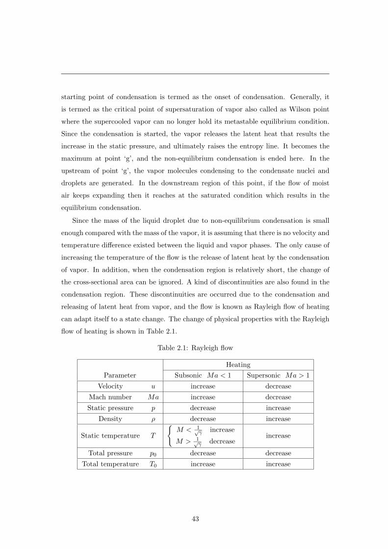
starting point of condensation is termed as the onset of condensation. Generally, it
is termed as the critical point of supersaturation of vapor also called as Wilson point
where the supercooled vapor can no longer hold its metastable equilibrium condition.
Since the condensation is started, the vapor releases the latent heat that results the
increase in the static pressure, and ultimately raises the entropy line. It becomes the
maximum at point ‘g’, and the non-equilibrium condensation is ended here. In the
upstream of point ‘g’, the vapor molecules condensing to the condensate nuclei and
droplets are generated. In the downstream region of this point, if the flow of moist
air keeps expanding then it reaches at the saturated condition which results in the
equilibrium condensation.
Since the mass of the liquid droplet due to non-equilibrium condensation is small
enough compared with the mass of the vapor, it is assuming that there is no velocity and
temperature difference existed between the liquid and vapor phases. The only cause of
increasing the temperature of the flow is the release of latent heat by the condensation
of vapor. In addition, when the condensation region is relatively short, the change of
the cross-sectional area can be ignored. A kind of discontinuities are also found in the
condensation region. These discontinuities are occurred due to the condensation and
releasing of latent heat from vapor, and the flow is known as Rayleigh flow of heating
can adapt itself to a state change. The change of physical properties with the Rayleigh
flow of heating is shown in Table 2.1.
Table 2.1: Rayleigh flow
Heating
Parameter Subsonic Ma < 1 Supersonic Ma > 1
Velocity u increase decrease
Mach number Ma increase decrease
Static pressure p decrease increase
Density ρ decrease increase
Static temperature T
M < 1√
γ increase
M > 1√γ decrease
increase
Total pressure p0 decrease decrease
Total temperature T0 increase increase
43

2. CONDENSATION PHENOMENA
According to the table, the heating phenomenon in a supersonic flow causes an
increase in the pressure and decrease of the flow velocity. The amount of increase in
the pressure and the decrease of velocity depend on the amount of heating. The Fig.
2.8 shows the typical Mach number distribution of the flow inside the one-dimensional
supersonic nozzle which is accompanied the latent heat release with non-equilibrium
condensation. The horizontal axis shows the distance along the nozzle axis, X , and
the vertical axis shows the Mach number, Ma. Q and Qcr, in the figure, show the
amount of latent heat released with condensation and the amount of heat required for
the thermal chocking1 of the flow, respectively.
When the isentropic expansion is occurred, condensation does not take place com-
pletely, the process moves along with the curved line af . While the degree of supersat-
uration (relative humidity) is gradually increased to downstream of the nozzle throat,
the Mach number decreases as shown by the curve aepg in Fig. 2.8 due to the com-
bined effect of releasing the latent heat and of expanding the area of condensation in
the nozzle. Here, the thermal choking doesn’t happen because of Q > Qcr. A weak
disturbance can be seen in the flow field due to the condensation. However, when the
degree of supersaturation in the nozzle gradually becomes larger, the starting point of
condensation gets near to the nozzle throat, and at a certain degree of supersaturation
it becomes Q = Qcr. At the point of occurring thermal choking Q = Qcr, the Mach
number approaches to the critical state. The distribution of Mach number, in that case,
can be represented by the curve adoh. If the degree of supersaturation still becomes
larger with Q > Qcr a shock wave mn is formed in the condensation region, and the
Mach number distribution becomes like the curve acmni in Fig. 2.8. It is seen that
the flow becomes subsonic just immediate downstream of the shock wave, but here the
effect of change of the condensation area is less than the effect of heat released due to
condensation, so that the Mach number is increased for this effect and the flow becomes
supersonic again. Thus, the shock wave generated due to condensation is called as the
condensation shock wave [Lai, 1993; Matsuo et al., 1984a, 1985b].
In Fig. 2.8, the curve acmni shows that the slope of Mach distribution (dMa/dx) is
negative at point m where the shock is formed, and if the effect of heating by the latent
1Thermal choking - For a subsonic flow or a supersonic flow, when it is heated Mach numberapproaches to unity and if the amount of heating become large then the Mach number reaches at thecritical state of Ma = 1. It is called choking due to heating or thermal choking.
44
heat release due to condensation is increased a stronger shock wave can be formed
adjusting the flow field. When the degree of supersaturation becomes considerably
larger, as shown by the curve abklj, the shock wave is formed at the point k where the
Mach slope (dMa/dx) becomes 0. In this case, although the effect of heating becomes
larger than the previous case, there is no stronger shock wave exists in the condensation
region and reaches to an unsteady state condition. Therefore, when the shock wave
is formed at point k to which the Mach slope (dMa/dx = 0), and if the value of Q
increases more and more, then the shock wave spreads to the upstream side and an
oscillation can be exhibited in the condensation region of the nozzle.
2.2.5 Flowfield oscillations by unsteady condensation shock wave
From the last discussion on condensation shock wave, when the degree of supersat-
uration becomes considerably higher and the effect of heating due to the release of
latent heat by condensation becomes considerably larger, there is no stronger shock
wave exists in the condensation region and reaches at the unsteady sate condition. In
the downstream of shock wave, the temperature being increased and consequently the
pressure is also increased and due to these effects the shock wave starts propagating
to the upstream, and in the downstream of propagating shock it becomes difficult to
condense again. Therefore, the amount of latent heat release is decreased, and the
change of heat release with time (dQ/dt) in the downstream region of the condensation
area becomes negative. As a result, the expansion wave is generated in the downstream
region. On the other hand, the shock wave that spreads to the upstream interferes with
this expansion wave, and is decelerated. In addition, this expansion wave is propagated
to the nozzle throat and it weakens by the effect of the flow passage area of the nozzle
when spreading to the upstream. Under the influence of the shock wave and of the
expansion wave which are decelerated and become weaker, the temperature falls and
the value of (dQ/dt) become positive in the downstream region, and it starts condens-
ing again. As a result, compression waves generate and formed a shock wave, and it
spreads to the upstream again. This way of generating the shock wave and expansion
wave, and propagating to the upstream region being repeated alternately creates an
oscillation in the nozzle flowfield [Matsuo et al., 1985b]. When one-cycle of this oscil-
lation is summarized, it becomes like the flow diagram in Fig. 2.9, and it consists of
the following four processes.
45

2. CONDENSATION PHENOMENA
(1) An increase in the amount of latent heat release due to condensation.
(2) Generation of the shock wave and spread to the upstream.
(3) A decrease in the amount of latent heat release due to condensation.
(4) Generation of the expansion wave and spread to the upstream.
In this section, the oscillation of the condensation shock wave in a simplest one-
dimensional supersonic nozzle is discussed only. In case of two-dimensional supersonic
nozzle, the influence of two-dimensional characteristics will appear in the condensation
shock wave. There are mainly three modes of oscillation of the condensation shock
wave [Adam & Schnerr, 1997], already discussed in the previous section 2.2.
2.3 Thermodynamics of condensation
Key feature is the release of latent heat in the condensation phenomena of condensing
gas by which it changes the amount of the state. Therefore, this section explains the
basic relational expressions such as equation of state etc. of moist air.
Assumptions are made for explaining the thermodynamic relations of condensation
as follows [Sislian, 1975]:
(1) The effect of molecular transport1 that causes the viscosity, the heat of conduction
and diffusion is neglected.
(2) Each elements of the operating gas, air or vapor, is thermally perfect2 and calor-
ically perfect3.
(3) The volume of droplet generated by condensation can be neglected for their ex-
tremely small volume in comparison with the entire volume.
(4) There is no velocity difference between the liquid phase (droplets) and the vapor
phase.
1Molecular transport - It includes the motion of the molecule, momentum transport in the form ofthe molecular viscosity, energy transport in the form of heat conduction and mass transport.
2Thermally perfect gas - It obeys the equation of state of the gas.3Calorically perfect gas - The specific heats at constant pressure cp and at constant volume cv are
always constant.
46
2.3.1 Mixture of gases with no condensation
Dalton’s law states, “Pressure of the gaseous mixture (total pressure) is equal to the
sum of pressures of each components of the gas mixture (partial pressure)”. Therefore,
the total pressure of the moist air is given by:
p = pa + pv (2.11)
Here,
pa =ma
V
<uni
MaT , pv =
mv
V
<uni
MvT
p =
(ma/V
Ma+mv/V
Mv
)<uniT (2.12)
where, V is the volume of the gaseous mixture, ma is the mass of air, mv is the mass of
vapor, T is the absolute temperature of the gaseous mixture, <uni is the universal gas
constant, and Ma, Mv are the molecular weight of air and water vapor, respectively.
Let us consider, Mm be the molecular weight and m(= ma +mv) be the total mass
of the mixture. Therefore, the total pressure can be given as follows:
p =m
V
<uni
MmT =
(ma
V+mv
V
)<uni
MmT (2.13)
Comparing Eqns. (2.12) and (2.13), it can be written as,(ma
V+mv
V
)1
Mm=ma/V
Ma+mv/V
Mv
(ma +mv)1
Mm=ma
Ma+mv
Mv
1
Mm=
ma
ma +mv
1
Ma+
mv
ma +mv
1
Mv(2.14)
Using the relation of specific humidity of Eqn. (2.4), the Eqn. (2.14) can be written
as follows:1
Mm= (1− mv
ma +mv)
1
Ma+
mv
ma + v
1
Mv
1
Mm= (1− ω)
1
Ma+ ω
1
Mv
Now, substituting the above equation to the Eqn. (2.13), the equation of state
47
2. CONDENSATION PHENOMENA
(equation of pressure) of the gaseous mixture can be written as,
p = ρm
((1− ω)
1
Ma+ ω
1
Mv
)<uniT (2.15)
However, the Mach number can be obtained from the speed of sound of the mixture,
a, and the speed of sound can be obtained from the entropy relation. In the present
study, it is assumed that the gaseous mixture is thermally and calorically perfect so
that the specific heat at constant pressure cp becomes constant, and it can be said that
cp = cp01. Thus, the speed of sound is given as follows:
a =
(γp
ρm
)1/2
=
(cp01
cp01 −<p
ρm
)1/2
=
(cp01
cp01 − <uniMm
p
ρm
)1/2
(2.16)
where, < is the gas constant of the gaseous mixture, and it becomes < = <uni. There-
fore, the Mach number M of the flow can be defined by the following expression.
M =u
a(2.17)
2.3.2 Mixture of gases with condensation
As the condensation occurs and drops of liquid (droplets) are existed in the gas mixture,
the mass equation of the mixture can be written as follows:
m = ma +mv +ml (2.18)
From Eqn. (2.8), the condensate mass fraction,
g =ml
m=
ml
ma +mv +ml(2.19)
Since the summation of masses of the liquid droplets and vapors (mv +ml = mv01)
present in the mixture is always constant, then
mv +ml
m=mv01
m= ω01 (2.20)
Now, using Eqns. (2.14), (2.19) and (2.20) the expression of the molecular weight
48
of the mixture which includes liquid droplets is given by the following equation.
1
Mm=m−mv01
m−ml
1
Ma+mv01 −ml
m−ml
1
Mv
1
Mm=
1− ω01
1− g1
Ma+ω01 − g1− g
1
Mv(2.21)
As the mass of the liquid droplets ml is included in the total volume V of the
mixture, the Eqn. (2.13) can be re-written as follows:
p =
(m−ml
V
)<uni
MmT =
(ρm −
ml
V
)<uni
MmT
= ρm
(1− ml
V ρm
)<uni
MmT = ρm
(1− ml
m
)<uni
MmT (2.22)
Using Eqn. (2.19), the Eqn. (2.22) can be written as:
p = ρm(1− g)<uni
MmT (2.23)
Substituting Eqn. (2.21) to Eqn. (2.23), the equation of state of the mixture which
contains the liquid droplets is given as follows:
p =
(1− ω01
Ma+ω01 − gMv
)ρm<uniT (2.24)
In this study, the frozen speed of sound af , the speed of sound in the non-equilibrium
condensation region, is employed to calculate the flow Mach number of the mixture and
it can be written in the following way [Matsuo et al., 1984a].
af =
(− ∂h/∂p
∂h/∂p− 1/ρ
)1/2
=
(cp01
cp01 − (1− g)<uniMm
p
ρm
)1/2
(2.25)
Generally, it is not possible to drive the equation of frozen speed of sound from the
entropy relation like the normal speed of sound. Therefore, the frozen Mach number
Mf of the flow is defined as follows:
Mf =u
af(2.26)
49
2. CONDENSATION PHENOMENA
Gibbs-Dalton law (it is the extension of Dalton’s law) states that “In a gaseous mix-
ture the property of any constituent is that which would be measured if that constituent
alone occupied the volume of the mixture i.e. without mutually interfering each other.
It follows that the property of the mixture is the sum of the corresponding properties
of the constituents”. The physical quantities of the gaseous mixture at the stagnation
condition is calculated according to the Gibbs-Dalton law, and the specific heat of the
gaseous mixture at constant pressure cp01 can be given as follows:
cp01 =ma
mcpa01 +
mv
mcpv01
Here, since the value of condensate mass fraction g is 0 at stagnation condition,
using the expression of specific humidity (Eqn. (2.4))it becomes as follows:
cp01 = (1− ω01)cpa01 + ω01cpv01 (2.27)
Similarly, the mass m01, the coefficient viscosity µ01, and the Prandtl number Pr01
of the gaseous mixture can be defined as follows:
m01 = (1− ω01)ma01 + ω01mv01 (2.28)
µ01 = (1− ω01)µa01 + ω01µv01 (2.29)
Pr01 = (1− ω01)Pra01 + ω01Prv01 (2.30)
2.4 Homogeneous nucleation
From the standpoint of unsteady kinetic theory, the condensation is a successive and
continuous process of nucleation. In a condensation process, it consists of condensation
of the vapor molecule which follows to the generation of condensate nuclei. However,
usually the condensate nuclei are considered to consist of a sufficiently large number of
molecules that they may be considered to form a liquid droplet. The condensation is
simply be classified into equilibrium and non-equilibrium condensation. On the other
hand, nucleation process also can be divided into homogeneous and heterogeneous nu-
cleation. In the present study, the focus is made on the non-equilibrium homogeneous
50
condensation. In addition, non-equilibrium condensation can be separated in two dis-
tinct processes, namely: homogeneous nucleation and droplet growth, as depicted in
Fig. 2.10. Homogeneous nucleation refers to the spontaneous formation, within the
vapor phase, of stable clusters by kinetic process of evaporation and impingement of
molecules; while droplet growth refers to the process in which stable droplets increase
in size by gaining more and more molecules. However, actually the generated clusters
are not only limited to grow up but also resolved by the collision. When the clusters
are repeating the collision then they are resolved by evaporation also.
According to the classical nucleation theory1, the generated cluster is assumed to be
one globe, and whether the cluster grow up, or they evaporate and resolved by collision
can possible to be judged from the size of cluster. The size which becomes a standard
cluster is called a critical cluster. In the classical theory of nucleation, the nucleation
rate is calculated based on the generation rate of this critical cluster. Moreover, a
bigger cluster than critical cluster can be generated and grow up in the nucleation
phenomena. The evaluation of the size of a critical cluster is a big problem because
it causes a marginal error on the critical cluster and also on the number order in this
nucleation rate.
In this section, the Frenkel formula using the liquid-drop model by capillary ap-
proximation of Gibbs is to be explained.
2.4.1 Generation of the cluster
A vapor consists of clusters of molecules bound together by their intermolecular in-
teractions. Nucleation from the vapor phase can be considered as a kinetic process
in which vapor molecules and their clusters combine with each other to form larger
clusters (dimmers, trimers,......, i-mers). The elementary process may be expressed as
a series of stepwise reactions consisting of bimolecular combination and unimolecular
1Classical nucleation theory (CNT) – the number of clusters is kept constant in the period ofadvancing the reaction in a system which is at the steady state condition.
51
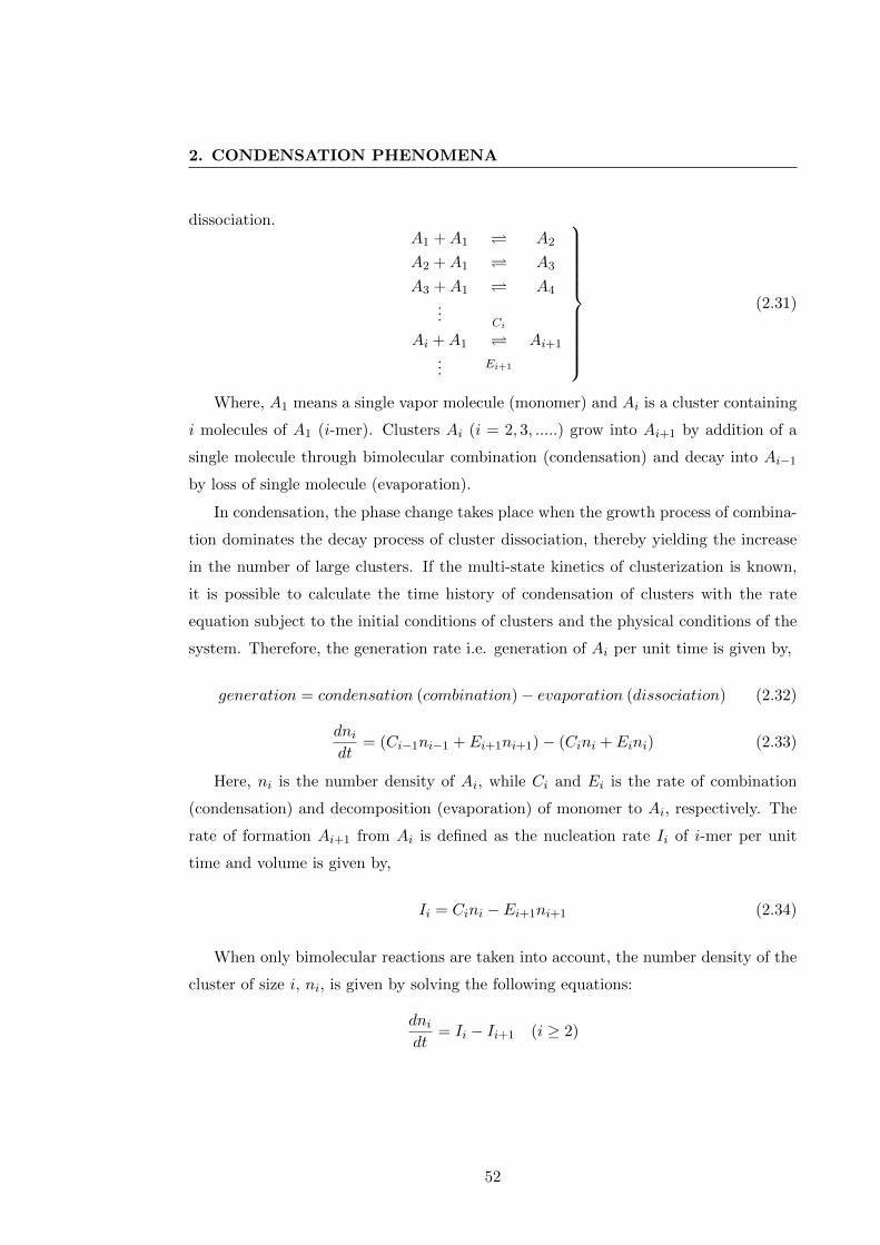
2. CONDENSATION PHENOMENA
dissociation.A1 +A1 A2
A2 +A1 A3
A3 +A1 A4
... Ci
Ai +A1 Ai+1
... Ei+1
(2.31)
Where, A1 means a single vapor molecule (monomer) and Ai is a cluster containing
i molecules of A1 (i-mer). Clusters Ai (i = 2, 3, .....) grow into Ai+1 by addition of a
single molecule through bimolecular combination (condensation) and decay into Ai−1
by loss of single molecule (evaporation).
In condensation, the phase change takes place when the growth process of combina-
tion dominates the decay process of cluster dissociation, thereby yielding the increase
in the number of large clusters. If the multi-state kinetics of clusterization is known,
it is possible to calculate the time history of condensation of clusters with the rate
equation subject to the initial conditions of clusters and the physical conditions of the
system. Therefore, the generation rate i.e. generation of Ai per unit time is given by,
generation = condensation (combination)− evaporation (dissociation) (2.32)
dnidt
= (Ci−1ni−1 + Ei+1ni+1)− (Cini + Eini) (2.33)
Here, ni is the number density of Ai, while Ci and Ei is the rate of combination
(condensation) and decomposition (evaporation) of monomer to Ai, respectively. The
rate of formation Ai+1 from Ai is defined as the nucleation rate Ii of i-mer per unit
time and volume is given by,
Ii = Cini − Ei+1ni+1 (2.34)
When only bimolecular reactions are taken into account, the number density of the
cluster of size i, ni, is given by solving the following equations:
dnidt
= Ii − Ii+1 (i ≥ 2)
52
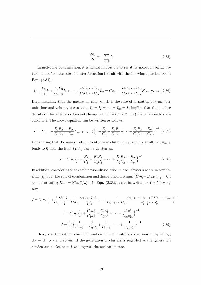
dnidt
= −∑i=2
Ii (2.35)
In molecular condensation, it is almost impossible to resist its non-equilibrium na-
ture. Therefore, the rate of cluster formation is dealt with the following equation. From
Eqn. (2.34),
I1 +E2
C2I2 +
E2E3
C2C3I3 + · · ·+ E2E2 · · ·Em
C2C3 · · ·CmIm = C1n1 −
E2E2 · · ·EmC2C3 · · ·Cm
Em+1nm+1 (2.36)
Here, assuming that the nucleation rate, which is the rate of formation of i-mer per
unit time and volume, is constant (I1 = I2 = · · · = Im = I) implies that the number
density of cluster ni also does not change with time (dni/dt = 0 ), i.e., the steady state
condition. The above equation can be written as follows:
I = (C1n1−E2E2 · · ·EmC2C3 · · ·Cm
Em+1nm+1)
1 +E2
C2+E2E3
C2C3+ · · ·+ E2E2 · · ·Em
C2C3 · · ·Cm
−1(2.37)
Considering that the number of sufficiently large cluster Am+1 is quite small, i.e., nm+1
tends to 0 then the Eqn. (2.37) can be written as,
I = C1n1
1 +
E2
C2+E2E3
C2C3+ · · ·+ E2E2 · · ·Em
C2C3 · · ·Cm
−1(2.38)
In addition, considering that combination-dissociation in each cluster size are in equilib-
rium (Iei ), i.e. the rate of combination and dissociation are same (Cinei−Ei+1n
ei+1 = 0),
and substituting Ei+1 = (Cinei )/n
ei+1 in Eqn. (2.38), it can be written in the following
way.
I = C1n1
1+
1
C2
C1ne1
ne2+
1
C2C3
C1C2ne1n
e2
ne2ne3
+· · ·+ 1
C2C3 · · ·CmC1C2 · · ·Cm−1n
e1n
e2 · · ·nem−1
ne1ne2 · · ·nem
−1
I = C1n1
1 +
C1ne1
C2ne2+C1n
e1
C3ne3+ · · ·+ C1n
e1
Cmnem
−1
I =n1
ne1
1
C1ne1+
1
C2ne2+
1
C3ne3+ · · ·+ 1
Cmnem
−1(2.39)
Here, I is the rate of cluster formation, i.e., the rate of conversion of A1 → A2,
A2 → A3 ,· · · and so on. If the generation of clusters is regarded as the generation
condensate nuclei, then I will express the nucleation rate.
53
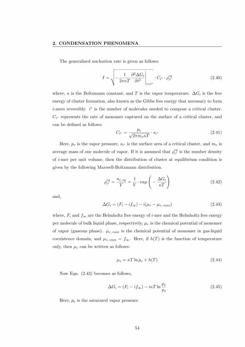
2. CONDENSATION PHENOMENA
The generalized nucleation rate is given as follows:
I =
√√√√− 1
2πκT
∂2∆Gi∂i2
∣∣∣∣∣i=i∗
· Ci∗ · ρeqi∗ (2.40)
where, κ is the Boltzmann constant, and T is the vapor temperature. ∆Gi is the free
energy of cluster formation, also known as the Gibbs free energy that necessary to form
i-mers reversibly. i∗ is the number of molecules needed to compose a critical cluster.
Ci∗ represents the rate of monomer captured on the surface of a critical cluster, and
can be defined as follows:
Ci∗ =pv√
2πmvκT· si∗ (2.41)
Here, pv is the vapor pressure, si∗ is the surface area of a critical cluster, and mv is
average mass of one molecule of vapor. If it is assumed that ρeqi∗ is the number density
of i-mer per unit volume, then the distribution of cluster at equilibrium condition is
given by the following Maxwell-Boltzmann distribution.
ρeqi∗ =ni, eqV
=1
V· exp
(− ∆Gi
κT
)(2.42)
and,
∆Gi = (Fi − if∞)− i(µv − µv, coex) (2.43)
where, Fi and f∞ are the Helmholtz free energy of i-mer and the Helmholtz free energy
per molecule of bulk liquid phase, respectively, µv is the chemical potential of monomer
of vapor (gaseous phase). µv, coex is the chemical potential of monomer in gas-liquid
coexistence domain, and µv, coex = f∞. Here, if h(T ) is the function of temperature
only, then µv can be written as follows:
µv = κT ln pv + h(T ) (2.44)
Now Eqn. (2.43) becomes as follows,
∆Gi = (Fi − if∞)− iκT lnpvps
(2.45)
Here, ps is the saturated vapor pressure.
54

2.4.2 Critical Cluster
The typical distributions of Gibbs free energy of formation of clusters (based on the Eqn.
(2.45)) at superheated, saturated, and supersaturated state are shown in Fig. 2.11. It
can be understood that below the saturated vapor pressure pv the Gibbs free energy
is increased monotonously. On the other hand, since ln(pv/ps) > 0 at supersaturated
state, ∆Gi might have the maximum value (Fig. 2.11). The cluster corresponding to
the maximum value of ∆Gi is called as the “critical cluster or critical nucleus
or critical embryo”, and has the lowest equilibrium concentration. Therfore, the
condition for critical cluster is as follows:
∂∆Gi∂i
∣∣∣∣∣i=i∗
= 0 (2.46)
Once clusters achieve this critical size, the addition of another molecule or monomer
to the cluster causes a decrease in the Gibbs free energy of cluster formation, as shown in
Fig. 2.11. In addition, when the monomer collides with the cluster of smaller size than
the critical cluster, dissociation (evaporation) of the cluster is occurred, and cluster size
decreases. On the other hand, when it collides with the cluster of larger size than the
critical cluster, combination (condensation) of the cluster is occurred, and grows to a
bigger cluster.
2.4.3 Frenkel’s nucleation rate
In order to materialize an expression of nucleation rate like Eqn. (2.40), it is necessary
to evaluate the Gibbs free energy of cluster formation by evaluating Fi in the Eqn.
(2.45). In classical nucleation theory, the liquid-drop model is used for calculating the
Fi, and i-mer is considered as one spherical bulk. The most simple liquid-drop model
is the Gibbs capillary approximation. In this model, the cluster of size i is regarded as
the macroscopic liquid-drop. Therefore, Fi becomes,
Fi = if∞ + σs1i2/3 + const (2.47)
where, σ is the gross surface tension, the 2nd term in the above equation represents the
surface energy required for the generation of cluster of size i. The 3rd term is chosen
55

2. CONDENSATION PHENOMENA
as −kT lnneq1 by the heuristic method. Therefore, comparing Eqns. (2.45) and (2.47),
and substituting to the relation of ρeqi in Eqn. (2.42), it can be written as follows:
ρeqi = ρeq1 exp
(− σs1
κTi2/3 + i ln(pv/ps∞)
)(2.48)
However, from Eqns. (2.40), (2.41) and (2.48), the expression of classical nucleation
rate Iclass can be written as follows:
Iclass =1
3
√θ
π
pvs1√2πmvκT
pvκT
exp
(− 4
27θ3 1
ln2(pv/ps)
)(2.49)
and,
θ =σs1
κT(2.50)
Here, if rc is introduced as the radius of critical cluster, then Eqn. (2.49) is trans-
formed into the following.
IF =1
ρl
√2mvσ
π
(pvκT
)2
exp
−4πr2
cσ
3κT
(2.51)
This IF is called as the Frenkel’s nucleation rate , and Eqn.(2.51) is known as the
Frenkel’s nucleation rate equation. However, the Frenkel’s nucleation rate equa-
tion is actually developed based on the classical nucleation theory of Volmer-Frenkel-
Zeldovich [Adam, 1996; Sislian, 1975] and this rate equation is also known as Volmer-
Frenkel-Zeldovich nucleation rate equation for their great contribution in developing the
theory of homogeneous nucleation. In addition, according to the definition of critical
cluster in Eqn.(2.46) the expression of rc is given by the following equation:
rc =2σ
ρl<vT ln(pv/ps,∞)(2.52)
Here, ρl is the density of condensate particle, <v is the gas constant of vapor. In
order to rectify the differences between the experimental and theoretical static pressure
distribution in a nozzle flow with non-equilibrium condensation, a correction factor Γ for
nucleation rate is introduced into this nucleation rate [Wegener & Wu, 1977]. Therefore,
56
Eqn. (2.51) becomes,
I = Γ · IF (2.53)
In the present study, the above expression of I is employed for calculating the nucleation
rate, and the value of the correction factor is taken as Γ = 106.
Till date, various formulae have been proposed for classical nucleation rate on the
basis of translation, rotation, vibration and internal degree of freedom of the cluster (for
example, Abraham [1974]). The nucleation rate equation of Frenkel [1946], that used
in the present study, is one of them. However, in solving the nucleation rate equation
a common problem have to take in account that is the surface tension of condensate
nuclei. In this regard, several algebraic equations have been proposed, like Tolman
[1949]. Generally, they use the power series for surface tension considering the effect
of droplet size. Therefore, depending on the droplet size the surface tension is often
expressed by the following equation.
σ =σ∞
1 + ar + b
r2
[a, b = const] (2.54)
Here, r is the radius of condensate particle, and σ∞ is the surface tension acting
on an infinitely flat surface of condensation. However, even though such a formula is
used it is difficult to say that the obtaining result is a satisfactory one. Therefore,
the most easy way to introduce a parameter ζ (coefficient of surface tension) in the
surface tension equation other than considering the effect of droplet size [Kawada &
Mori, 1972; Krickwood & Buff, 1949; Oriani & Sundquist, 1963]. Therefore, the surface
tension equation becomes as follows:
σ = ζσ∞ (2.55)
Though, there are various methods of deciding the value of surface tension coefficient
ζ, most suitable one is to obtain from experiment. In addition, based on experiments
there are some empirical formulae of surface tension in an infinite plane surface. Among
them, the formula of surface tension in an infinite plane surface [Mundinger, 1994]
57
2. CONDENSATION PHENOMENA
proposed by Schnerr and Dohrmann (1990) is used in the present study, as follows:
σ∞(T ) =
76.1 + 0.155× (273.15− T ) × 10−3 (T ≥ 249.39K)
(1.1313− 3.7091× 10⁻³ × T )× 10−4 − 5.6464 × 10⁻⁶ (T < 249.39K)
(2.56)
This expression is a function of temperature. However, from some previous study,
the result obtained without using the coefficient of surface tension and by substituting
the surface tension of liquid droplet σ∞(T ) in an infinite plane surface to the σ in Eqn.
(2.52) is relatively more identical with the experimental data.
2.5 Droplet Growth
Once a cluster or condensate nuclei is formed that is able to grow, its further growth is
determined by a droplet growth law which expresses the increment of mass of a critical
droplet as it moves downstream with flow. It is assumed that each droplets grows
separately and does not coalesce with others, and has the same velocity and temperature
as the surrounding gaseous medium. Furthermore, some previous estimates showed
that the molecular mean free path of the condensing vapor in air is 2 ∼ 5 × 10⁻⁴ cm
in thermodynamic state where the droplet begins to grow. The radius of a critical
cluster (Eqn. (2.52)) is two or three orders of magnitude less than the mean free path.
Moreover, the average droplet size is usually less than one mean free path after passing
through the condensation zone [Sislian, 1975]. Therefore, the droplet growth must be
computed on the basis of free-molecular flow (λ≫ r).
The kinetics of vapor-liquid phase transition (condensation and evaporation) has
been the subject of numerous studies beginning with Hertz (1882) and Knudsen (1915).
The equation for the net mass flow in unit time of vapor molecules condensing on
a spherical droplet, usually called the Hertz-Knudsen equation [Sislian, 1975]. This
section describes the condensation rate equations showing the growth rate of a cluster
and the rate of total amount of condensation.
2.5.1 Growth rate of the cluster
In Eqn. (2.41), the rate of monomer captured on the surface of a critical cluster has
already been shown. This expression for the size of the cluster, when the cluster size
is sufficiently smaller than mean free path of the vapor, is obtained from the kinetic
58
theory of gases in which the distribution of cluster follows the Maxwell-Boltzmann
velocity distribution law. In similar way, the rate of monomer captured (condensation)
per unit volume Ci, i.e. the amount of monomer captured on the cluster per unit time
and per unit volume, can be calculated with the following expression.
Ci =pv√
2πmvκT(2.57)
where i is the size of the cluster, pv is the partial pressure of vapor, and T is the
temperature.
On one hand, if ps is assigned as the saturated vapor pressure at the droplet tem-
perature Ts, then the rate of monomer dissociation (evaporation) from the cluster per
unit volume, Ei can be defined as follows:
Ei =ps√
2πmvκTs(2.58)
Therefore, the net mass of the monomer is captured on the cluster per unit time
and unit volume can be given as follows:
m = 4πr2ξc(Ci − Ei)
= 4πr2ξc
(pv√
2πmvκT− ps√
2πmvκTs
)(2.59)
Here, this equation is generally known as the Hertz-Knudsen formula, and r in the
equation represents the radius of the cluster. In addition, although ξc is called as the
condensation coefficient [Mills & Seban, 1967; Pound, 1972], when monomer collides
with a cluster it represents the rate of combination and dissociation. Furthermore, if it
is assuming that the cluster and gas phase are in local equilibrium (T = Ts), then Eqn.
2.59 can also be expressed by the rate of change of cluster radius, and the resulting
equation is the growth rate equation of cluster, as follows:
dr
dt= ξc
ps
(pvps− 1)
ρl√
2π<vT(2.60)
The condensation coefficient may be given as a function of temperature (for ex-
ample, Young [1982]), and in some cases it may not have temperature dependency.
59
2. CONDENSATION PHENOMENA
However, according to the study of Mundinger [1994], using the saturated vapor pres-
sure ps, r of liquid droplet of radius r the expression for the growth rate of the cluster
can be given as follows:dr
dt= ξc
pv − ps, rρl√
2π<vT(2.61)
Here,
ps, r = ps,∞ exp
(2σ∞ρl<vTr
)(2.62)
Mundinger [1994] has been reported that without the use of condensation coefficient
the results also suitably fitted with the experimental data. Therefore, the value of
condensation coefficient ξc = 1.0 was used in the present study.
Addendum
Succeeding discussion concerns with the relationship between the coefficients regard-
ing the non-equilibrium condensation (such as, surface tension coefficient, condensation
coefficient and nucleation coefficient) and onset of condensation [Matsuo et al., 1984b].
• Influence of surface tension coefficient : If the value of the coefficient of
surface tension ζ is reduced, the point of onset of non-equilibrium condensation
tends to approach to the nozzle throat. As seen from Eqns. (2.52) and (2.54),
at low surface tension the critical radius of condensate nuclei become small, and
the condensate nuclei are likely to be formed by the combined effect of molecular
coalescence-decomposition of vapor molecules at lower degree of supersaturation.
• Influence of condensation coefficient : The onset of condensation tends to
approach to the nozzle throat with the increase in the value of the condensation
coefficient ξc. In addition, the maximum value of nucleation rate at the onset
of condensation becomes smaller with higher value of condensation coefficient.
The larger condensation coefficient increases the molecular collision-combination
as well as increases the growth rate of liquid droplets, and the rate of capturing
the vapor molecule is also increased that results in decreasing the number of
condensate nuclei necessary for starting the condensation.
• Influence of nucleation coefficient: The higher value of nucleation coefficient
tends to move the onset of condensation towards the nozzle throat like surface
60
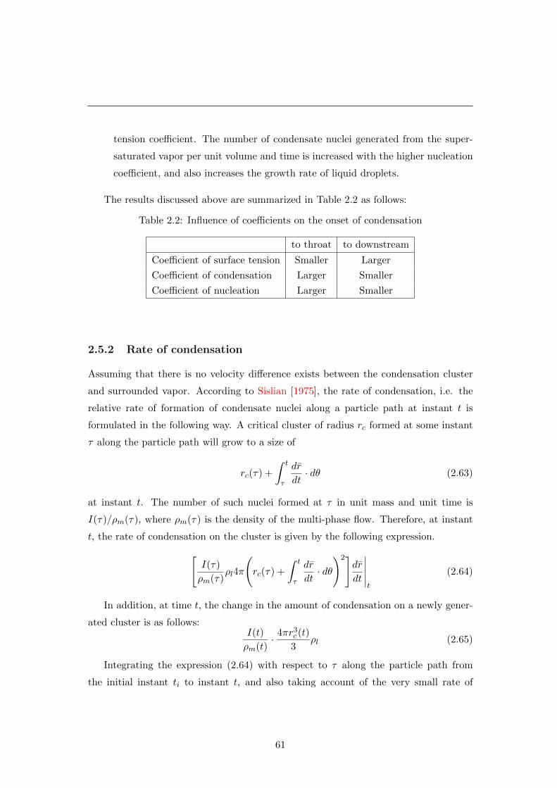
tension coefficient. The number of condensate nuclei generated from the super-
saturated vapor per unit volume and time is increased with the higher nucleation
coefficient, and also increases the growth rate of liquid droplets.
The results discussed above are summarized in Table 2.2 as follows:
Table 2.2: Influence of coefficients on the onset of condensation
to throat to downstream
Coefficient of surface tension Smaller Larger
Coefficient of condensation Larger Smaller
Coefficient of nucleation Larger Smaller
2.5.2 Rate of condensation
Assuming that there is no velocity difference exists between the condensation cluster
and surrounded vapor. According to Sislian [1975], the rate of condensation, i.e. the
relative rate of formation of condensate nuclei along a particle path at instant t is
formulated in the following way. A critical cluster of radius rc formed at some instant
τ along the particle path will grow to a size of
rc(τ) +
∫ t
τ
dr
dt· dθ (2.63)
at instant t. The number of such nuclei formed at τ in unit mass and unit time is
I(τ)/ρm(τ), where ρm(τ) is the density of the multi-phase flow. Therefore, at instant
t, the rate of condensation on the cluster is given by the following expression.[I(τ)
ρm(τ)ρl4π
(rc(τ) +
∫ t
τ
dr
dt· dθ
)2]dr
dt
∣∣∣∣∣t
(2.64)
In addition, at time t, the change in the amount of condensation on a newly gener-
ated cluster is as follows:I(t)
ρm(t)· 4πr3
c (t)
3ρl (2.65)
Integrating the expression (2.64) with respect to τ along the particle path from
the initial instant ti to instant t, and also taking account of the very small rate of
61

2. CONDENSATION PHENOMENA
condensation at t, due to nucleation, the following equation of the rate of production
of the new phase (condensate mass) can be obtained.
dg
dt= 4πρl
[I(t)
ρm(t)
r3c (t)
3+dr
dt
∫ t
ti
I(τ)
ρm(τ)
(rc(τ) +
∫ t
τ
dr
dt· dθ
)2dτ
](2.66)
dg
dt=
ρlρm
4π
3r3cI + ρmD1
dr
dt
(2.67)
dD1
dt=
4πr2cI
ρm+D2
dr
dt(2.68)
dD2
dt=
8πrcI
ρm+D3
dr
dt(2.69)
dD3
dt=
8πI
ρm(2.70)
where, g is the condensate mass fraction, and D1, D2, D3 are merely variables intro-
duced to the integro-differential Eqn. (2.66) to four simultaneous first-order differential
equations [Hill, 1966].
According to Hill [1966], r, the mean radius of liquid droplet, is given by the fol-
lowing way, and in Eqn. (2.62) it is used as the radius.
r =
√2D1
D3(2.71)
2.6 Change of entropy due to condensation
During the rapid expansion of condensing gas such as moist air, vapor, etc. in a su-
personic nozzle the non-equilibrium condensation is taken place. This is an irreversible
process which accompanies the increase of entropy which leads to the loss of total pres-
sure in the flowfield. The formula that shown the change of entropy of in the gaseous
mixture due to condensation in the moist air [Matsuo, 1988] can be written as follows:
∆s = s− s01 = (1− ω01)<Ma
ln
(T γa/(γa−1)
Pa
)︸ ︷︷ ︸
Entropy of air
62

+ (ω01 − g)<Mv
ln
(T γv/(γv−1)
Pv
)︸ ︷︷ ︸
Entropy of vapor
+ g
(−1
γ
3
ρl
∂σ
∂T
)︸ ︷︷ ︸
Entropy of liquid
(2.72)
Here, s, ω01, and σ are the entropy per unit mass, initial specific humidity, and
surface tension, respectively. In the right-hand side of Eqn. (2.72), 1st, 2nd and 3rd
terms are the entropy of air, vapor and liquid droplet, respectively. Particularly 3rd
term is not regarded as the entropy of liquid droplet, but only considers the entropy
at the surface of minute droplet. Moreover, in case of vapor only, it becomes ω01=1 in
Eqn. (2.72).
Here, if s01 is assumed as the entropy at stagnation condition of the nozzle entrance,
the relation between the entropy and total pressure loss becomes like the following
expression.s− s01
cp= ln
(T0
T01
)− R/M
cpln
(p0
p01
)(2.73)
where, cp , M shows the specific heat at constant pressure and molecular weight of
the gaseous mixture; T0, p0 shows the local temperature and total pressure; and T01
, p01 shows the temperature and total pressure at the stagnation condition of nozzle
entrance.
Moreover, assuming the adiabatic flow T0/T01 is become 1, and the expression for
the change of entropy will become as follows:
∆s
R/M=s− s01
R/M= ln
(p01
p0
)(2.74)
2.7 Conclusion
in this chapter, a review is presented of the modeling of non-equilibrium condensation
for a mixture of water vapor and carrier gas. the fundamental idea of splitting the
condensation process into a nucleation and droplet growth process dates back to Os-
watitsch [1942]. The Frenkel formula of nucleation based on the classical nucleation
theory using the liquid-drop model by capillary approximation of Gibbs discussed in
63

2. CONDENSATION PHENOMENA
detail. The droplet growth equation, and the relation of change of entropy due to the
non-equilibrium condensation have also reported.
64

Figure 2.3: Schlieren picture of an asymmetric periodic oscillating flow through a su-personic nozzle A1 [Adam, 1996]
65

2. CONDENSATION PHENOMENA
(a) p− v diagram
(b) T − s diagram
Figure 2.4: sketch of the non-equilibrium condensation process in a schematic p − vand T − s diagram
66
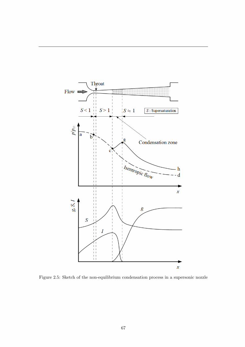
Figure 2.5: Sketch of the non-equilibrium condensation process in a supersonic nozzle
67

2. CONDENSATION PHENOMENA
Figure 2.6: Schlieren streak recording of the different mode of oscillation in nozzle S2.Adam & Schnerr [1997]
68
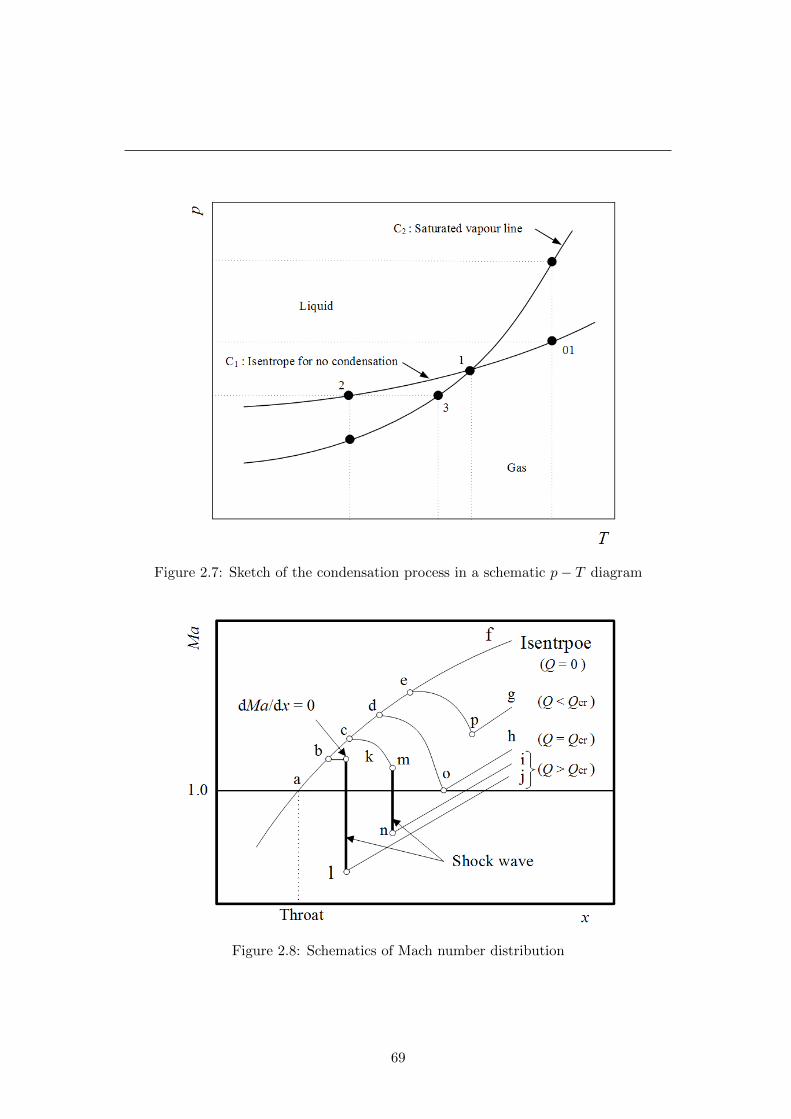
Figure 2.7: Sketch of the condensation process in a schematic p− T diagram
Figure 2.8: Schematics of Mach number distribution
69
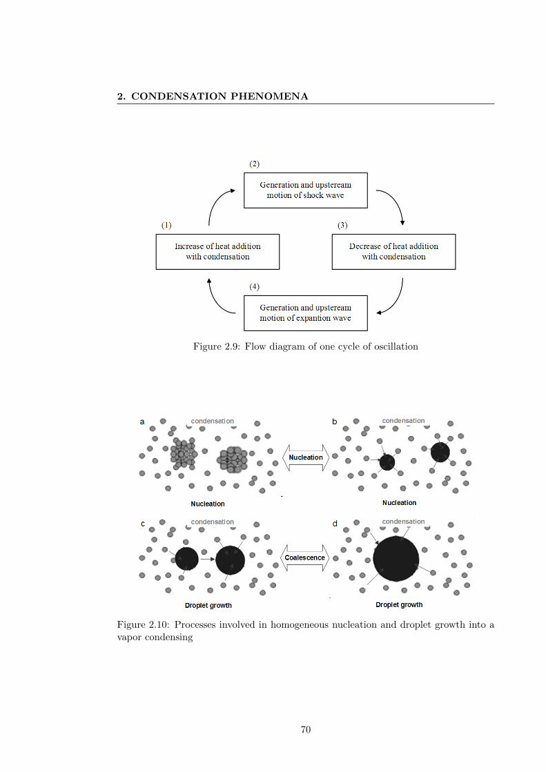
2. CONDENSATION PHENOMENA
Figure 2.9: Flow diagram of one cycle of oscillation
Figure 2.10: Processes involved in homogeneous nucleation and droplet growth into avapor condensing
70
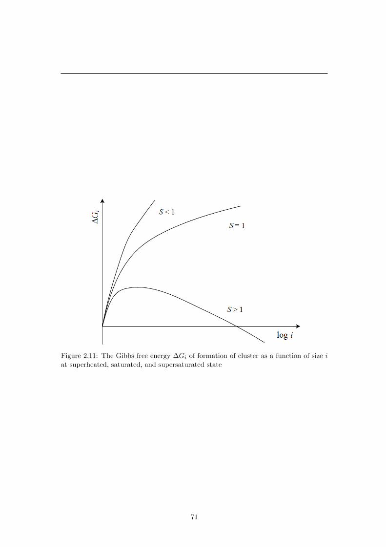
Figure 2.11: The Gibbs free energy ∆Gi of formation of cluster as a function of size iat superheated, saturated, and supersaturated state
71

2. CONDENSATION PHENOMENA
72
Chapter 3
Physical and mathematical
modeling
3.1 Introduction
The present study describe a detail of the physical mechanisms underlying effect of
non-equilibrium condensation on self-sustained oscillation in supersonic impinging jets.
Computational Fluid Dynamic (CFD) study was employed to numerically simulate
the flow. In order to analyze the flow of supersonic impinging moist air jets, the
solution of the Navier-Stokes equations is required. Because of complexity in the flow
of supersonic impinging jets and the strong viscous effects, it is impossible to obtain
an analytical solution of the Navier-Stokes equations for practical configurations. Thus
numerical techniques have to be used to solve those equations. In this chapter, a detail
about governing equations and turbulence modeling employed in the present study are
documented. However, the thermophysical properties and relational expressions about
the thermophysical properties used in the present study are presented in Appendix A.
3.2 Governing equations
The Navier-Stokes equations are a set of partial differential equations for the conserva-
tion of mass, momentum, and energy. These may be derived by applying the principle
of classical mechanics and thermodynamics. These equations are based on Newton’s
hypothesis, that the normal and shear stresses are linear functions of the rates of de-
73

3. PHYSICAL AND MATHEMATICAL MODELING
formation, and that the thermodynamic pressure is equal to the negative of one-third
the sum of the normal stresses.
3.2.1 Governing equations in Cartesian coordinates
For simplicity of the present two-phase flow computational analysis, several assump-
tions are made; there is no velocity slip and no temperature difference between con-
densate particles and gas mixtures, the effect of of the particles on the pressure field
can be neglected with reasonable accuracy. The governing equations are the unsteady
compressible Navier-Stokes equations, turbulence kinetic energy, and eddy viscosity
equations coupled with the rate form of liquid-phase production equations [Sislian,
1975]. The divergence form of governing equations written in Cartesian coordinates (x,
r) system without external body forces or outside heat addition are as follows:
∂U
∂t+∂E
∂x+∂F
∂r=∂R
∂x+∂S
∂r+
1
rH 1 + H 2 + Q (3.1)
where U is the vector of conservative variables, which include density, velocities, etc.
E and F are the inviscid flux vectors; and R and S are the viscous flux vectors in the
x and r directions, respectively. r is the vertical distance from the axis. H 1, H 2 and
Q are the source terms for axisymmetry, turbulence and condensation, respectively.
These vectors can be expressed by following equations in matrix form
U =
ρm
ρmu
ρmv
Et
ρmk
ρmR
ρmg
ρmD1
ρmD2
ρmD3
, E =
ρmu
ρmu2 + p
ρmuv
u(Et + p)
ρmuk
ρmuR
ρmug
ρmuD1
ρmuD2
ρmuD3
, F =
ρmv
ρmuv
ρmv2 + p
v(Et + p)
ρmvk
ρmvR
ρmvg
ρmvD1
ρmvD2
ρmvD3
(3.2)
74
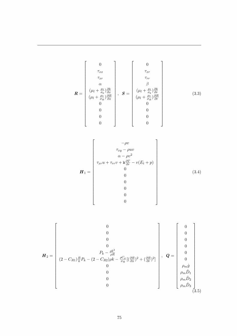
R =
0
τxx
τxr
α
(µl + µtσk
)∂k∂x(µl + µt
σR)∂R∂x
0
0
0
0
, S =
0
τxr
τrr
β
(µl + µtσk
)∂k∂r(µl + µt
σR)∂R∂r
0
0
0
0
(3.3)
H 1 =
−ρvτxy − ρuvα− ρv2
τxru+ τrrv + k∂T∂r − v(Et + p)
0
0
0
0
0
0
(3.4)
H 2 =
0
0
0
0
Pk − ρk2
ρR
(2− CR1)Rk Pk − (2− CR2)ρk − ρCµσR
[(∂R∂x )2 + (∂R∂r )2]
0
0
0
0
, Q =
0
0
0
0
0
0
ρmg
ρmD1
ρmD2
ρmD3
(3.5)
75
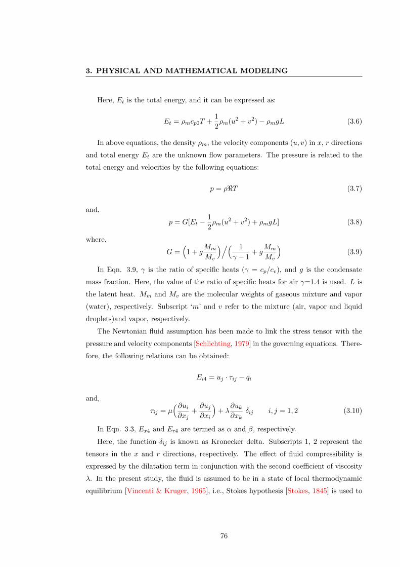
3. PHYSICAL AND MATHEMATICAL MODELING
Here, Et is the total energy, and it can be expressed as:
Et = ρmcp0T +1
2ρm(u2 + v2)− ρmgL (3.6)
In above equations, the density ρm, the velocity components (u, v) in x, r directions
and total energy Et are the unknown flow parameters. The pressure is related to the
total energy and velocities by the following equations:
p = ρ<T (3.7)
and,
p = G[Et −1
2ρm(u2 + v2) + ρmgL] (3.8)
where,
G =(
1 + gMm
Mv
)/( 1
γ − 1+ g
Mm
Mv
)(3.9)
In Eqn. 3.9, γ is the ratio of specific heats (γ = cp/cv), and g is the condensate
mass fraction. Here, the value of the ratio of specific heats for air γ=1.4 is used. L is
the latent heat. Mm and Mv are the molecular weights of gaseous mixture and vapor
(water), respectively. Subscript ‘m’ and v refer to the mixture (air, vapor and liquid
droplets)and vapor, respectively.
The Newtonian fluid assumption has been made to link the stress tensor with the
pressure and velocity components [Schlichting, 1979] in the governing equations. There-
fore, the following relations can be obtained:
Ei4 = uj · τij − qi
and,
τij = µ(∂ui∂xj
+∂uj∂xi
)+ λ
∂uk∂xk
δij i, j = 1, 2 (3.10)
In Eqn. 3.3, Ex4 and Er4 are termed as α and β, respectively.
Here, the function δij is known as Kronecker delta. Subscripts 1, 2 represent the
tensors in the x and r directions, respectively. The effect of fluid compressibility is
expressed by the dilatation term in conjunction with the second coefficient of viscosity
λ. In the present study, the fluid is assumed to be in a state of local thermodynamic
equilibrium [Vincenti & Kruger, 1965], i.e., Stokes hypothesis [Stokes, 1845] is used to
76
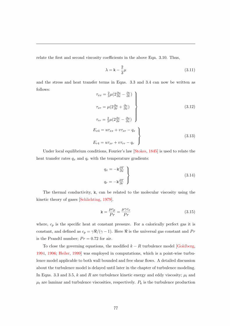
relate the first and second viscosity coefficients in the above Eqn. 3.10. Thus,
λ = k− 2
3µ (3.11)
and the stress and heat transfer terms in Eqns. 3.3 and 3.4 can now be written as
follows:τxx = 2
3µ(2∂u∂x −∂v∂r )
τxr = µ(2∂u∂r + ∂v∂x)
τrr = 23µ(2∂v∂r −
∂u∂x)
(3.12)
Ex4 = uτxx + vτxr − qx
Er4 = uτxr + vτrr − qr
(3.13)
Under local equilibrium conditions, Fourier’s law [Stokes, 1845] is used to relate the
heat transfer rates qx and qr with the temperature gradients:
qx = −k∂T∂x
qr = −k∂T∂r
(3.14)
The thermal conductivity, k, can be related to the molecular viscosity using the
kinetic theory of gases [Schlichting, 1979].
k =µcpPr
=µγcvPr
(3.15)
where, cp is the specific heat at constant pressure. For a calorically perfect gas it is
constant, and defined as cp = γ</(γ− 1). Here < is the universal gas constant and Pr
is the Prandtl number; Pr = 0.72 for air.
To close the governing equations, the modified k −R turbulence model [Goldberg,
1994, 1996; Heiler, 1999] was employed in computations, which is a point-wise turbu-
lence model applicable to both wall bounded and free shear flows. A detailed discussion
about the turbulence model is delayed until later in the chapter of turbulence modeling.
In Eqns. 3.3 and 3.5, k and R are turbulence kinetic energy and eddy viscosity; µl and
µt are laminar and turbulence viscosities, respectively. Pk is the turbulence production
77
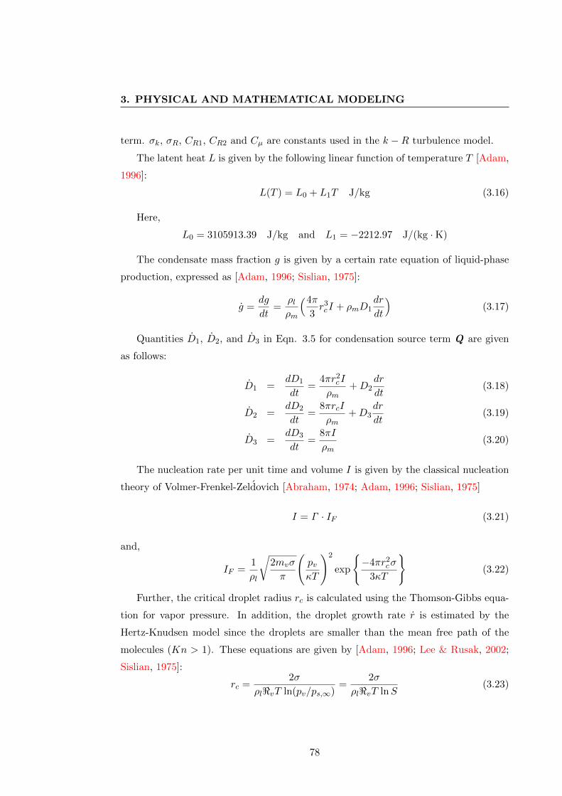
3. PHYSICAL AND MATHEMATICAL MODELING
term. σk, σR, CR1, CR2 and Cµ are constants used in the k −R turbulence model.
The latent heat L is given by the following linear function of temperature T [Adam,
1996]:
L(T ) = L0 + L1T J/kg (3.16)
Here,
L0 = 3105913.39 J/kg and L1 = −2212.97 J/(kg ·K)
The condensate mass fraction g is given by a certain rate equation of liquid-phase
production, expressed as [Adam, 1996; Sislian, 1975]:
g =dg
dt=
ρlρm
(4π
3r3cI + ρmD1
dr
dt
)(3.17)
Quantities D1, D2, and D3 in Eqn. 3.5 for condensation source term Q are given
as follows:
D1 =dD1
dt=
4πr2cI
ρm+D2
dr
dt(3.18)
D2 =dD2
dt=
8πrcI
ρm+D3
dr
dt(3.19)
D3 =dD3
dt=
8πI
ρm(3.20)
The nucleation rate per unit time and volume I is given by the classical nucleation
theory of Volmer-Frenkel-Zeldovich [Abraham, 1974; Adam, 1996; Sislian, 1975]
I = Γ · IF (3.21)
and,
IF =1
ρl
√2mvσ
π
(pvκT
)2
exp
−4πr2
cσ
3κT
(3.22)
Further, the critical droplet radius rc is calculated using the Thomson-Gibbs equa-
tion for vapor pressure. In addition, the droplet growth rate r is estimated by the
Hertz-Knudsen model since the droplets are smaller than the mean free path of the
molecules (Kn > 1). These equations are given by [Adam, 1996; Lee & Rusak, 2002;
Sislian, 1975]:
rc =2σ
ρl<vT ln(pv/ps,∞)=
2σ
ρl<vT lnS(3.23)
78

r =dr
dt=ξcρl
pv − ps,r√2π<vT
(3.24)
In the above equations, κ, mv, ps,∞, pv, <v, S and σ are the Boltzmann constant,
molecular weight of vapor, saturated vapor pressure of a infinite flat surface, vapor
pressure, gas constant of water vapor, degree of supersaturation and surface tension,
respectively [Adam, 1996; Sislian, 1975]. Subscript ‘l’ refers to the liquid phase. Γ [We-
gener & Wu, 1977] and ξc [Mills & Seban, 1967; Pound, 1972] are the accommodation
coefficient for nucleation and condensation, respectively. Surface tension σ [Sislian,
1975; Wegener & Wu, 1977] is given by using the the surface tension of an infinite
flat-film σ∞ and the coefficient of surface tension ζ [Kawada & Mori, 1972; Krickwood
& Buff, 1949; Kwon et al., 1988; Oriani & Sundquist, 1963] as follows:
σ = ζσ∞ (3.25)
In the present study, values chosen for Γ , ξc and ζ are
Γ = 106, ξc = 1.0, ζ = 1.0 (3.26)
The density of the liquid phase is given by the following function of temperature
[Adam, 1996; Prupacher & Klett, 1997]:
ρl(T ) =
(A0+A1t+A2t2+A3t3+A4t4+A5t5)
1+B0t(kg/m3) (T ≥ 0C)
(A6 +A7t+A8t2) (kg/m3) (T < 0C)
(3.27)
where, t is the temperature in C and the coefficients are given by:
A0 = 999.8396 A5 = −393.2952× 10⁻¹²
A1 = 18.224944 A6 = 999.84
A2 = −7.92221× 10⁻³ A7 = 0.086
A3 = −55.44846× 10⁻⁶ A8 = −0.0108
A4 = 149.7562× 10⁻⁹ B0 = 18.159725× 10⁻³
79
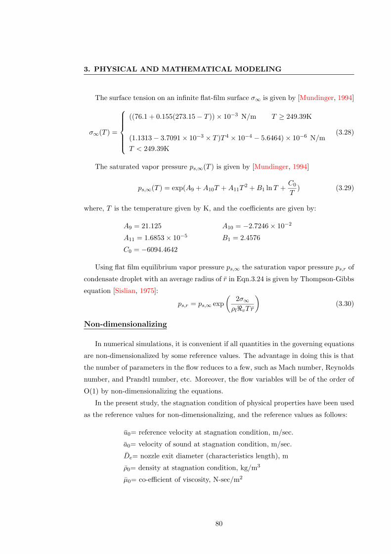
3. PHYSICAL AND MATHEMATICAL MODELING
The surface tension on an infinite flat-film surface σ∞ is given by [Mundinger, 1994]
σ∞(T ) =
((76.1 + 0.155(273.15− T ))× 10−3 N/m T ≥ 249.39K
(1.1313− 3.7091× 10⁻³ × T )T 4 × 10⁻⁴ − 5.6464)× 10−6 N/m
T < 249.39K
(3.28)
The saturated vapor pressure ps,∞(T ) is given by [Mundinger, 1994]
ps,∞(T ) = exp(A9 +A10T +A11T2 +B1 lnT +
C0
T) (3.29)
where, T is the temperature given by K, and the coefficients are given by:
A9 = 21.125 A10 = −2.7246× 10⁻²
A11 = 1.6853× 10⁻⁵ B1 = 2.4576
C0 = −6094.4642
Using flat film equilibrium vapor pressure ps,∞ the saturation vapor pressure ps,r of
condensate droplet with an average radius of r in Eqn.3.24 is given by Thompson-Gibbs
equation [Sislian, 1975]:
ps,r = ps,∞ exp
(2σ∞ρl<vT r
)(3.30)
Non-dimensionalizing
In numerical simulations, it is convenient if all quantities in the governing equations
are non-dimensionalized by some reference values. The advantage in doing this is that
the number of parameters in the flow reduces to a few, such as Mach number, Reynolds
number, and Prandtl number, etc. Moreover, the flow variables will be of the order of
O(1) by non-dimensionalizing the equations.
In the present study, the stagnation condition of physical properties have been used
as the reference values for non-dimensionalizing, and the reference values as follows:
u0= reference velocity at stagnation condition, m/sec.
a0= velocity of sound at stagnation condition, m/sec.
De= nozzle exit diameter (characteristics length), m
ρ0= density at stagnation condition, kg/m3
µ0= co-efficient of viscosity, N-sec/m2
80

p0= stagnation pressure, Pa
T0= stagnation temperature, K
The non-dimensional flow variables are expressed as follows:
u∗ = u/u0 v∗ = v/u0
x∗ = x/De y∗ = y/De
t∗ = t/(De/u0) ρ∗ = ρ/ρ0
T ∗ = T /T0 p∗ = p/(ρ0u20) = p/(γp0M
20 )
µ∗ = µ/µ0 κ∗ = κ/µ0
e∗ = e/u02 E∗t = Et/(ρ0u2
0)
a∗ = a/a0 λ∗ = κ∗ − 2µ∗/3
D∗ = ∂u∗/∂x∗ + ∂v∗/∂y∗ and so on.
where, the non-dimensional variables are denoted by an asterisk (*). Since the velocity
at stagnation is u0 = 0, then the reference velocity u0 can be represented by the sound
speed at stagnation condition a0. Substituting the non-dimensional variables into the
Eqn. 3.1, an equation very similar to Eqn. 3.1 is obtained, but there are two non-
dimensional coefficients that appear in front of the viscous terms. These coefficients
are the Mach and Reynolds numbers, which are defined as follows:
M0 =u0
a0=a0
a0= 1 and Re0 =
ρ0u0De
µ0(3.31)
Therefore, the non-dimensionalized governing equations can be given as follows:
∂U
∂t+∂E
∂x+∂F
∂r=
1
Re0
(∂R
∂x+∂S
∂r
)+
1
rH 1 + H 2 + Q (3.32)
For a detailed description and expression of the non-dimensional equations, the reader
is referred to Ref. [Tannehill et al., 1997]. In the following discussions, all variables (ρ,
u, v, p, etc.) are non-dimensional. The asterisk has been dropped for convenience.
3.2.2 Transformation to generalized coordinates
To obtain solutions for the flow past arbitrary geometries and handle arbitrary motions,
a body-fitted coordinate system is desired so that the boundary surfaces in the physical
plane can be easily mapped onto planes or lines in the computational domain. The
81
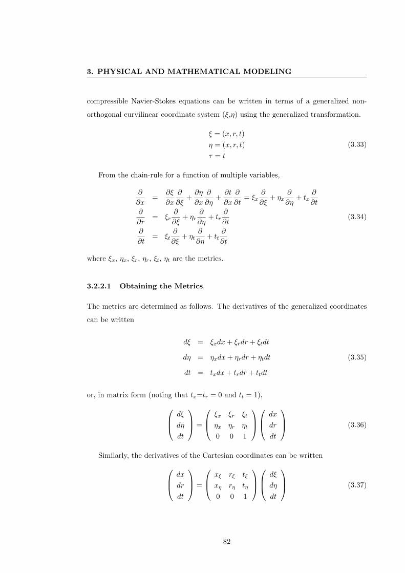
3. PHYSICAL AND MATHEMATICAL MODELING
compressible Navier-Stokes equations can be written in terms of a generalized non-
orthogonal curvilinear coordinate system (ξ,η) using the generalized transformation.
ξ = (x, r, t)
η = (x, r, t)
τ = t
(3.33)
From the chain-rule for a function of multiple variables,
∂
∂x=
∂ξ
∂x
∂
∂ξ+∂η
∂x
∂
∂η+∂t
∂x
∂
∂t= ξx
∂
∂ξ+ ηx
∂
∂η+ tx
∂
∂t
∂
∂r= ξr
∂
∂ξ+ ηr
∂
∂η+ tr
∂
∂t(3.34)
∂
∂t= ξt
∂
∂ξ+ ηt
∂
∂η+ tt
∂
∂t
where ξx, ηx, ξr, ηr, ξt, ηt are the metrics.
3.2.2.1 Obtaining the Metrics
The metrics are determined as follows. The derivatives of the generalized coordinates
can be written
dξ = ξxdx+ ξrdr + ξtdt
dη = ηxdx+ ηrdr + ηtdt (3.35)
dt = txdx+ trdr + ttdt
or, in matrix form (noting that tx=tr = 0 and tt = 1), dξ
dη
dt
=
ξx ξr ξt
ηx ηr ηt
0 0 1
dx
dr
dt
(3.36)
Similarly, the derivatives of the Cartesian coordinates can be written dx
dr
dt
=
xξ rξ tξ
xη rη tη
0 0 1
dξ
dη
dt
(3.37)
82

Therefore, it is evident that ξx ξr ξt
ηx ηr ηt
0 0 1
=
xξ rξ tξ
xη rη tη
0 0 1
−1
(3.38)
The determinant of the inverse matrix represented on the right-hand side of Eqn.
3.38 is ∣∣∣∣∣∣∣xξ rξ tξ
xη rη tη
0 0 1
∣∣∣∣∣∣∣ = xξrη − rξxη (3.39)
The Jacobian of the transformation is defined to be
J =∂(x, r, t)
∂(ξ, η, t)=
∣∣∣∣∣∣∣xξ rξ tξ
xη rη tη
0 0 1
∣∣∣∣∣∣∣ (3.40)
And,
1
J=∂(x, r, t)
∂(ξ, η, t)=
∣∣∣∣∣∣∣ξx ξr ξt
ηx ηr ηt
0 0 1
∣∣∣∣∣∣∣ (3.41)
Therefore, the metrics are
ξx =1
Jrη ηx = − 1
Jrξ ξr = − 1
Jxη ηr =
1
Jxξ (3.42)
In addition,
xξ = Jηr xη = −Jξr rξ = −Jηx rη = Jξx (3.43)
3.2.2.2 Applying the Transformation
Applying the transformation to the Eqn. 3.32, the following non-dimensional governing
equations in the curvilinear coordinate system can be obtained.
U τ + E ξ + F η =1
Re0
(Rξ + F η
)+
1
rH 1 + H 2 + Q (3.44)
83
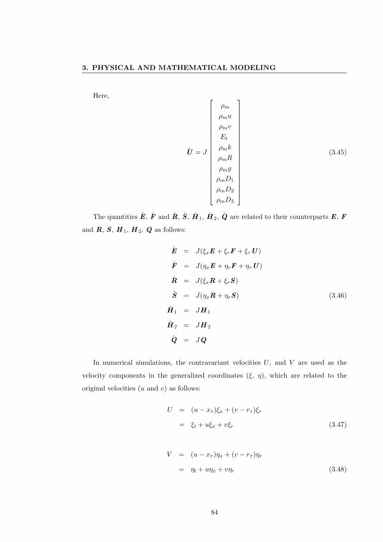
3. PHYSICAL AND MATHEMATICAL MODELING
Here,
U = J
ρm
ρmu
ρmv
Et
ρmk
ρmR
ρmg
ρmD1
ρmD2
ρmD3
(3.45)
The quantities E , F and R, S , H 1, H 2, Q are related to their counterparts E , F
and R, S , H 1, H 2, Q as follows:
E = J(ξxE + ξrF + ξτU )
F = J(ηxE + ηrF + ητU )
R = J(ξxR + ξrS)
S = J(ηxR + ηrS) (3.46)
H 1 = JH 1
H 2 = JH 2
Q = JQ
In numerical simulations, the contravariant velocities U , and V are used as the
velocity components in the generalized coordinates (ξ, η), which are related to the
original velocities (u and v) as follows:
U = (u− xτ )ξx + (v − rτ )ξr
= ξt + uξx + vξr (3.47)
V = (u− xτ )ηx + (v − rτ )ηr
= ηt + uηx + vηr (3.48)
84

where,
ξt = −xτξx − rτξrηt = −xτηx − rτηr
(3.49)
The contravariant velocity components U and V are constant in directions normal
to ξ and η surfaces, respectively. The quantity xτ and yτ are the velocity of any points
on the “grid” in an initial frame. In the present work, the body is not in motion and
these velocities are zero.
The inviscid fluxes E , F ; viscous flux vectors R, R; and source terms H 1, H 2, Q
in the transformed coordinate system are:
E = J
ρmU
ρmuU + ξxp
ρmvU + ξrp
(Et + p)U
ρmkU
ρmRU
ρmgU
ρmD1U
ρmD2U
ρmD3U
, F = J
ρmV
ρmuV + ηxp
ρmvV + ηrp
(Et + p)V
ρmkV
ρmRV
ρmgV
ρmD1V
ρmD2V
ρmD3V
(3.50)
R =
0
ξxτxx + ξrτrx
ξxτxr + ξrτrr
ξxα+ ξrβ
(µl + µtσk
)(ξxkx + ξrkr)
(µl + µtσR
)(ξxRx + ξrRr)
0
0
0
0
, S =
0
ηxτxx + ηrτrx
ηxτxr + ηrτrr
ηxα+ ηrβ
(µl + µtσk
)(ηxkx + ηrkr)
(µl + µtσR
)(ηxRx + ηrRr)
0
0
0
0
(3.51)
85

3. PHYSICAL AND MATHEMATICAL MODELING
H 1 = J
−ρvτxy − ρuvα− ρv2
τxru+ τrrv + k∂T∂r − v(Et + p)
0
0
0
0
0
0
(3.52)
H 2 = J
0
0
0
0
Pk − ρk2
ρR
(2− CR1)Rk Pk − (2− CR2)ρk − ρCµσR
(R2x +R2
r)
0
0
0
0
, Q = J
0
0
0
0
0
0
ρmg
ρmD1
ρmD2
ρmD3
(3.53)
The viscous flux terms with the shear stresses in the transformed coordinates are:
τxx =2
3µ [2(uξξx + uηηx)− (vξξr + vηηr)]
τxr = µ (uξξr + uηηr) + vξξx + vηηx) (3.54)
τrr =2
3µ [2(vξξr + vηηr)− (uξξx + uηηx)]
where the Stokes hypothesis for bulk viscosity has been used, as discussed earlier. The
auxiliary functions are:
α = τxxu+ τxrv +µ
(γ − 1)Pr
∂T
∂x
= τxxu+ τxrv +µ
(γ − 1)Pr
(ξx∂a2
∂ξ+ ηx
∂a2
∂η
)(3.55)
86
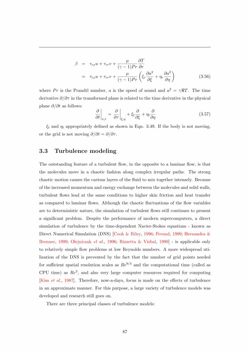
β = τrxu+ τrrv +µ
(γ − 1)Pr
∂T
∂r
= τrxu+ τrrv +µ
(γ − 1)Pr
(ξr∂a2
∂ξ+ ηr
∂a2
∂η
)(3.56)
where Pr is the Prandtl number, a is the speed of sound and a2 = γ<T . The time
derivative ∂/∂τ in the transformed plane is related to the time derivative in the physical
plane ∂/∂t as follows:∂
∂t
∣∣∣∣x,r
=∂
∂τ
∣∣∣∣ξ,η
+ ξt∂
∂ξ+ ηt
∂
∂η(3.57)
ξt and ηt appropriately defined as shown in Eqn. 3.49. If the body is not moving,
or the grid is not moving ∂/∂t = ∂/∂τ .
3.3 Turbulence modeling
The outstanding feature of a turbulent flow, in the opposite to a laminar flow, is that
the molecules move in a chaotic fashion along complex irregular paths. The strong
chaotic motion causes the carious layers of the fluid to mix together intensely. Because
of the increased momentum and energy exchange between the molecules and solid walls,
turbulent flows lead at the same conditions to higher skin friction and heat transfer
as compared to laminar flows. Although the chaotic fluctuations of the flow variables
are to deterministic nature, the simulation of turbulent flows still continues to present
a significant problem. Despite the performance of modern supercomputers, a direct
simulation of turbulence by the time-dependent Navier-Stokes equations - known as
Direct Numerical Simulation (DNS) [Cook & Riley, 1996; Freund, 1999; Hernandez &
Brenner, 1999; Olejniczak et al., 1996; Rizzetta & Visbal, 1999] - is applicable only
to relatively simple flow problems at low Reynolds numbers. A more widespread uti-
lization of the DNS is prevented by the fact that the number of grid points needed
for sufficient spatial resolution scales as Re9/4 and the computational time (called as
CPU time) as Re3, and also very large computer resources required for computing
[Kim et al., 1987]. Therefore, now-a-days, focus is made on the effects of turbulence
in an approximate manner. For this purpose, a large variety of turbulence models was
developed and research still goes on.
There are three principal classes of turbulence models:
87

3. PHYSICAL AND MATHEMATICAL MODELING
1. Reynolds-average Navier-Stokes (RANS) models
This model is based on equations obtained by averaging the equation of motion
over time, over a coordinate in which the mean flow does not vary, or over an
ensemble of realizations (an imagined set of flows in which all controllable factors
are kept fixed). This approach is also called as one-point closure and leads to
a set of partial differential equations called the Reynolds-average Navier-Stokes
(RANS) equations. The complexity of turbulence makes it unlikely that any
single Reynolds-averaged model will be able to represent all turbulent flows, so
turbulence models should be regarded as engineering approximations rather than
scientific laws. This model can also be classified as follows:
(a) Eddy-viscosity hypothesis
(b) Reynolds stress models
2. Large Eddy Simulation (LES)
LES is based on the observation that the small turbulent structures are more
universal in character than the large eddies. Therefore, the idea is to compute the
contributions of the large, energy-carrying structures to momentum and energy
transfer and to model the effects of the small structures.
3. Direct Numerical Simulation (DNS)
The most accurate approach to turbulence simulation is to solve the Navier-Stokes
equations without averaging or approximation other than numerical discretiza-
tions whose errors can be estimated and controlled. It is also the simplest ap-
proach from the conceptual point of view. In such simulations, all of the motions
contained in the flow are resolved. The computed flow field obtained is equivalent
to a single realization of a flow or a short-duration experiment, this approach is
called direct numerical simulation (DNS).
In this research, to make an easy computing condition that means to reduce the com-
putational time, and at the same time for the simplicity to adopt, the Eddy-viscosity
hypothesis of RANS (Reynolds Average Navier-Stokes System of equations) is em-
ployed. The system equations are derived by decomposing the flow variables in the
conservation equations into time-mean and fluctuating components, and then time av-
eraging the entire Navier-Stokes equations.
88
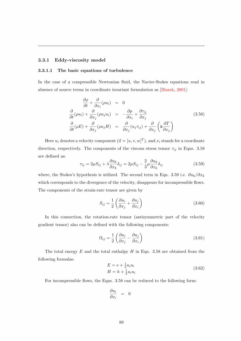
3.3.1 Eddy-viscosity model
3.3.1.1 The basic equations of turbulence
In the case of a compressible Newtonian fluid, the Navier-Stokes equations read in
absence of source terms in coordinate invariant formulation as [Blazek, 2001]:
∂ρ
∂t+
∂
∂xi(ρui) = 0
∂
∂t(ρui) +
∂
∂xj(ρujui) = − ∂p
∂xi+∂τij∂xj
(3.58)
∂
∂t(ρE) +
∂
∂xj(ρujH) =
∂
∂xj(ujτij) +
∂
∂xj
(k∂T
∂xj
)Here ui denotes a velocity component (~u = [u, v, w]T ), and xi stands for a coordinate
direction, respectively. The components of the viscous stress tensor τij in Eqns. 3.58
are defined as:
τij = 2µSij + λ∂uk∂xk
δij = 2µSij −2
3µ∂uk∂xk
δij (3.59)
where, the Stokes’s hypothesis is utilized. The second term in Eqn. 3.59 i.e. ∂uk/∂xk
which corresponds to the divergence of the velocity, disappears for incompressible flows.
The components of the strain-rate tensor are given by
Sij =1
2
(∂ui∂xj
+∂uj∂xi
)(3.60)
In this connection, the rotation-rate tensor (antisymmetric part of the velocity
gradient tensor) also can be defined with the following components:
Ωij =1
2
(∂ui∂xj− ∂uj∂xi
)(3.61)
The total energy E and the total enthalpy H in Eqn. 3.58 are obtained from the
following formulae.
E = e+ 12uiui
H = h+ 12uiui
(3.62)
For incompressible flows, the Eqns. 3.58 can be reduced to the following form:
∂ui∂xi
= 0
89
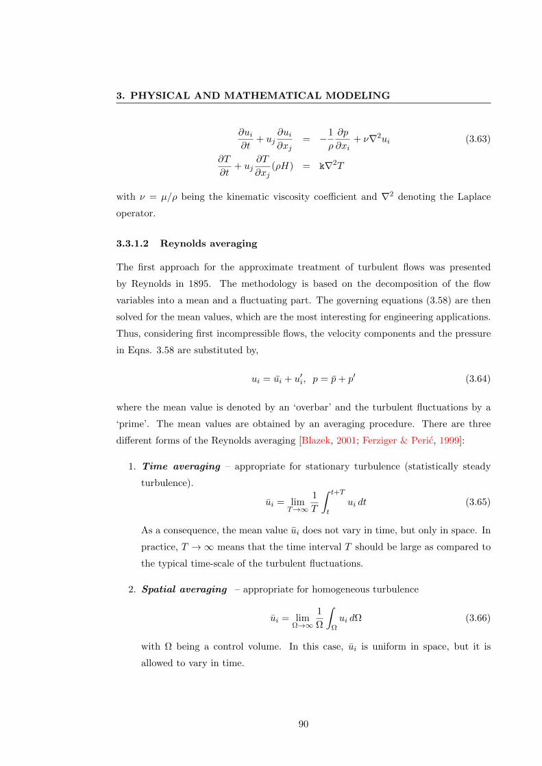
3. PHYSICAL AND MATHEMATICAL MODELING
∂ui∂t
+ uj∂ui∂xj
= −1
ρ
∂p
∂xi+ ν∇2ui (3.63)
∂T
∂t+ uj
∂T
∂xj(ρH) = k∇2T
with ν = µ/ρ being the kinematic viscosity coefficient and ∇2 denoting the Laplace
operator.
3.3.1.2 Reynolds averaging
The first approach for the approximate treatment of turbulent flows was presented
by Reynolds in 1895. The methodology is based on the decomposition of the flow
variables into a mean and a fluctuating part. The governing equations (3.58) are then
solved for the mean values, which are the most interesting for engineering applications.
Thus, considering first incompressible flows, the velocity components and the pressure
in Eqns. 3.58 are substituted by,
ui = ui + u′i, p = p+ p′ (3.64)
where the mean value is denoted by an ‘overbar’ and the turbulent fluctuations by a
‘prime’. The mean values are obtained by an averaging procedure. There are three
different forms of the Reynolds averaging [Blazek, 2001; Ferziger & Peric, 1999]:
1. Time averaging – appropriate for stationary turbulence (statistically steady
turbulence).
ui = limT→∞
1
T
∫ t+T
tui dt (3.65)
As a consequence, the mean value ui does not vary in time, but only in space. In
practice, T →∞ means that the time interval T should be large as compared to
the typical time-scale of the turbulent fluctuations.
2. Spatial averaging – appropriate for homogeneous turbulence
ui = limΩ→∞
1
Ω
∫Ωui dΩ (3.66)
with Ω being a control volume. In this case, ui is uniform in space, but it is
allowed to vary in time.
90

3. Ensemble averaging – appropriate for general turbulence.
ui = limN→∞
1
N
N∑m=1
ui (3.67)
Here, the mean value ui still remains a function of time and space coordinates.
For all three approaches, the average of the fluctuating part is zero i.e. u′i = 0.
However, it can be easily seen that u′iu′i 6= 0. The same is true for u′iu
′j , if both
turbulent velocity components are correlated.
3.3.1.3 Mass averaging
In cases where the density is not constant (for compressible flows), it is advisable to
apply the density (mass) weighted or Favre decomposition [Favre, 1965a,b] to cer-
tain quantities in Eqns. 3.58 instead of Reynolds averaging. Otherwise, the averaged
governing equations would become considerably more complicated due to additional
correlations involving density fluctuations. The most convenient way is to employ
Reynolds averaging for density and pressure, and Favre averaging for other variables
such as velocity, internal energy, enthalpy and temperature. Favre averaged quantities,
for example the velocity components, are obtained from the following relation [Favre,
1965a,b]:
ui =1
ρlimT→∞
1
T
∫ t+T
tρui dt (3.68)
where ρ denotes the Reynolds-averaged density. Hence, the Favre decomposition reads
ui = ui + u′′i (3.69)
where ui represents the mean value and u′′i the fluctuating part of the velocity ui. Again,
the average of the fluctuating part is zero, i.e. u′′i = 0. Furthermore, the average of
the product of two fluctuating quantities is not zero, if the quantities are correlated.
Hence, for example, u′′i u′′i 6= 0 and in general u′′i u
′′j 6= 0. The following relationships can
be derived for a mix between Favre and Reynolds averaging:
ρui = ρui, ρu′′i = 0 but u′′i 6= 0 (3.70)
91
3. PHYSICAL AND MATHEMATICAL MODELING
3.3.1.4 Reynolds-averaged Navier-Stokes equations
For incompressible flow :
Applying either the time averaging equation (Eqn. 3.65) or the ensemble averaging
equation (Eqn. 3.67) to the incompressible Navier-Stokes equations (Eqn. 3.63), the
following relations for the mass and momentum conservation can be obtained.
∂ui∂xi
= 0
ρ∂ui∂t
+ uj∂ui∂xj
= − ∂p
∂xi+
∂
∂xj
(τij − ρu′iu′j
)(3.71)
These are known as the Reynolds-Averaged Navier-Stokes equations (RANS) for in-
compressible flow. The Eqn. 3.71 are formally identical to the Navier-Stokes equations
(Eqn. 3.58) or (Eqn. 3.63) with the exception of the additional term,
τRij = −ρu′iu′j = −ρ(uiuj − uiuj) (3.72)
which constitutes the so-called Reynolds-stress tensor. It represents the transfer of
momentum due to turbulent fluctuations. The laminar viscous stresses are evaluated
according to Eqns. (3.59) and (3.60) using Reynolds-averaged velocity components,
i.e.,
τij = 2µSij = 2µ
(∂ui∂xj
+∂uj∂xi
)(3.73)
The Reynolds-stress tensor in 3D consists of nine components:
ρu′iu′j =
ρ(u′)2 ρu′v′ ρu′w′
ρv′u′ ρ(v′)2 ρv′w′
ρw′u′ ρw′v′ ρ(w′)2
(3.74)
However, since u′i and u′j in the correlations can be interchanged, the Reynolds-
stress tensor contains only six independent components. The sum of the normal stresses
divided by density defines the turbulent kinetic energy, i.e.,
k =1
2u′iu′i =
1
2
[(u′)2 + (v′)2 + (w′)2
](3.75)
For compressible flow :
92
In turbulence modeling, it is quite common to assume that Morkovin’s hypothesis
[Morkovin, 1964] is valid. It states that the turbulent structure of a boundary layer is
not notably influenced by density fluctuations if ρ′ ρ. This is generally true for wall-
bounded flows up to a Mach number of about five. However, in the case of hypersonic
flows or for compressible free shear layers, density fluctuations have to be taken into
account. The same holds also for flows with combustion or significant heat transfer.
Application of the Reynolds averaging (Eqn. 3.65 or 3.67) to density and pressure,
and of the Favre averaging equation (Eqn. 3.68) to the remaining flow variables in the
compressible Navier-Stokes equations (Eqn. 3.58) yields [Wilcox, 1993],
∂ρ
∂t+
∂
∂xi(ρui) = 0
∂
∂t(ρui) +
∂
∂xj(ρuj ui) = − ∂p
∂xi+
∂
∂xj
(τij − ρu′′i u′′j
)∂
∂t(ρE) +
∂
∂xj(ρujH) =
∂
∂xj
(k∂T
∂xj− ρu′′jh′′ + τiju′′j − u′′jk
)(3.76)
+∂
∂xj
(ui(τij − ρu′′i u′′j )
)These are the Favre- and Reynolds-Averaged Navier-Stokes equations. Similarly,
to the Reynolds averaging, the viscous stress tensor in the momentum (and energy)
equation is extended by the Favre-averaged Reynolds-stress tensor, i.e.,
τFij = −ρu′′i u′′j (3.77)
It’s form is similar to Eqn. 3.74 with Favre instead of Reynolds averaging. The
components of the laminar (molecular) viscous stress tensor τij are evaluated by Eqn.
3.59 using Favre-averaged velocity components. Now, employing the definition of the
Favre-averaged the turbulent kinetic energy and total energy in Eqn. 3.76, and the
total enthalpy can be expressed as:
ρk =1
2ρu′′i u
′′i
ρE = ρe+1
2ρuiui +
1
2ρu′′i u
′′i = ρe+
1
2ρuiui + ρk (3.78)
ρH = ρh+1
2ρuiui +
1
2ρu′′i u
′′i = ρh+
1
2ρuiui + ρk
93
3. PHYSICAL AND MATHEMATICAL MODELING
The individual parts of the Favre- and Reynolds-averaged Navier-Stokes equations
(Eqn. 3.76) have the following physical meaning citepWilcox1993:
∂
∂xj
(k∂T
∂xj
)− molecular diffusion of heat
∂
∂xj
(ρu′′jh
′′)− turbulent transport of heat
∂
∂xj
(τiju′′j
)− molecular diffusion of k
∂
∂xj
(ρu′′jk
)− turbulent transport of k
∂
∂xj(uj τij) − work done by the molecular stresses
∂
∂xj
(ujτ
Fij
)− work done by the Favre− averaged Reynolds stresses
The molecular diffusion and turbulent transport of k are very often neglected. This
is a valid approximation for transonic and supersonic flows.
3.3.1.5 Eddy-viscosity hypothesis
One of the most significant contributions to turbulence modeling was presented in 1877
by Boussineq [Blazek, 2001; Ferziger & Peric, 1999; Hirsch, 1998]. It’s based on the
observation that the momentum transfer in a turbulent flow is dominated by the mixing
caused by the large energetic turbulent eddies. The Boussineq hypothesis assumes that
the turbulent shear stress is related to mean rate of stain, as in a laminar flow. The
proportionality factor is the eddy viscosity. The Boussineq hypothesis for Reynolds
averaged incompressible flow can be written as:
τRij = −ρu′iu′j = 2µtSij −2
3ρkδij (3.79)
where, Sij denotes the Reynolds-averaged stain-rate tensor, k is the turbulent kinetic
energy (k = 12u′iu′i ), and µt stands for the eddy viscosity. Unlike the molecular viscosity
µ, the eddy viscosity µt represents no physical characteristics of the fluid, but it is a
function of the local flow conditions. Additionally, µt is also strongly affected by flow
history effects. In the case of the compressible Favre- and Reynolds-averaged Navier-
94
Stokes equations (Eqn. 3.76), the Boussineq eddy-viscosity hypothesis reads,
τFij = −ρu′′i u′′j = 2µtSij −2µt3
∂uk∂xk
δij −2
3ρkδij (3.80)
where, sij and k are the Favre-averaged stain-rate and turbulent kinetic energy, respec-
tively. However, the term 23ρkδij is often neglected, particularly in connection with
simpler turbulence models (like algebraic ones). The approximation, which is com-
monly used for the modeling of the turbulent heat-flux vector, is based on the classical
Reynolds analogy. Hence, it can be written as:
ρu′′jh′′ = −kt
∂T
∂xj(3.81)
with the turbulent thermal conductivity coefficient,
kt = cpµtPrt
(3.82)
In Eqn. 3.82, cp denotes the specific heat at constant pressure and Prt is the
turbulent Prandtl number. The turbulent Prandtl number is in general assumed to be
constant over the flow field. By applying the eddy-viscosity approach to the Reynolds-
and Favre averaged form of the governing equations (Eqn. 3.76 or 3.58), the dynamic
viscosity coefficient µ in the viscous stress tensor equation (Eqn. 3.72 or 3.59) is simply
replaced by the sum of a laminar and a turbulent component, i.e.,
µ = µl + µt (3.83)
In this present study, the laminar viscosity µl is computed with the aid of the
Sutherland’s law [Shames, 1992] and the formula is given as follows:
µlµl0
=
(T
T0
)3/2 T0 +B
T +B(3.84)
where, µl0 is some known viscosity at absolute temperature T0 and B is a constant
determined by curve fitting. Furthermore, according to the Reynolds analogy given by
Eqn. 3.81 the coefficient of thermal conductivity k is evaluated as:
k = kl + kt = cp
(µlPrl
+µtPrt
)(3.85)
95
3. PHYSICAL AND MATHEMATICAL MODELING
The eddy-viscosity concept of Boussineq is, at least from engineering point of view,
very attractive since it requires ‘only’ the determination of µt (the turbulent kinetic
energy k needed for the term 23ρkδij in Eqn. 3.79 or 3.80 is either obtained as a by-
product of the turbulence model or is simply omitted). Since, the eddy viscosity µt is
the only unknown parameter; a turbulence model is needed to evaluate the value of
µt. There are several turbulence models used in CFD to evaluate the value of the eddy
viscosity µt to simulate the turbulent flow. However, most of them are just good under
some specific flow situations. A proper choice of turbulence models is important and can
have a large effect on the accuracy of the simulations. The modified k −R turbulence
model [Goldberg, 1996; Yamamoto & Daiguji, 1991] , which is a two-equation model
pointwise turbulence model applicable to both wall bounded and free shear flows, is
employed in the present study.
3.3.2 Modified k −R turbulence model
The modeling of turbulence in near-wall regions usually involves distance to wall as
an explicit parameter in the formulation in zero equation models, such as in Baldwin-
Lomax (1978) turbulence model. When dealing with the complex flows involving mul-
tiple surfaces, the notion of the wall distance becomes difficult to define properly and
is often cumbersome to implement. It is therefore, necessity of a model which, while
applicable all the way to solid surfaces, does not involve wall distance explicitly. On
the way of this journey, a two-equation turbulence model for near wall regions, named
as k − R model, was proposed by Baldwin and Barth in 1990. After that, Goldberg
[1994] was proposed a modified version of the Baldwin-Barth k − R two-equation tur-
bulence model, in which the near-wall function fµ is based on the ratio of the large
eddy and the Kolmogorov time scale. This result that the modified k−R two-equation
turbulence model of Goldberg [1994] is applicable to both wall-bounded and free shear
flows which, nevertheless, does not require explicit knowledge of local distance to walls,
rendering it useful within both structured and unstructured computational frameworks
for flow predictions involving complex geometries. In 1996, a three-equation R− k − εturbulence model was proposed by Goldberg [1996] in order to make it applicable to
arbitrary flow topologies. Here, in this section, a short description on the modified
k −R turbulence model [Adam, 1996; Heiler, 1999] is documented.
96

3.3.2.1 Transport equations
In orthogonal coordinate system :
∂U
∂t+∂E
∂x+∂F
∂r=∂R
∂x+∂S
∂r+ H (3.86)
Here,
U =
[ρk
ρR
], E =
[ρuk
ρuR
], F =
[ρvk
ρvR
]
R =
(µl + µtσk
)∂k∂x
(µl + µtσR
)∂R∂x
, S =
(µl + µtσk
)∂k∂r
(µl + µtσR
)∂R∂r
H =
Pk − ρk2
ρR
(2− CR1)Rk Pk − (2− CR2)ρk − ρCµσR
[(∂R∂x )2 + (∂R∂r )2]
where σk, σR, CR1, CR2, Cµ are constants, and H is the source term for turbulence.
In Goldberg (1994) two-equation turbulence model the modification to the standard
k− ε model, introduced by Launder-Sharma (1974), was done by replacing k2/R as the
dissipation term instead of ε.
The turbulence production term Pk is given in terms of the Boussinesq concept
Pk =
[µt(
∂ui∂xj
+∂uj∂xi− 2
3
∂uk∂xk
δij)−2
3ρkδij
]∂ui∂xj
(3.87)
In the present work, two-dimensional form of this equation is used, and can be written
as follows:
Pk = µt
[2(u2
x + v2r ) + (ur + vx)2 − 2
3(ux + vr)
2
]− 2
3ρk(ux + vr) (3.88)
The eddy viscosity field is given by,
µt ≡ ρνt = ρCµfµR (3.89)
where, the near-wall damping function fµ is given as
fµ =tanh(α′Ret)
tanh(β′Ret)(3.90)
97
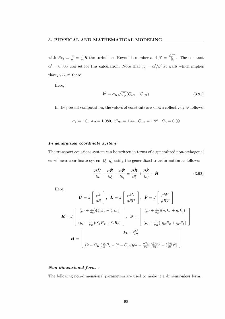
3. PHYSICAL AND MATHEMATICAL MODELING
with Ret ≡ Rνl
= ρµlR the turbulence Reynolds number and β′ =
C3/4µ
2k . The constant
α′ = 0.005 was set for this calculation. Note that fµ = α′/β′ at walls which implies
that µt ∼ y4 there.
Here,
k2 = σR√Cµ(CR2 − CR1) (3.91)
In the present computation, the values of constants are shown collectively as follows:
σk = 1.0, σR = 1.080, CR1 = 1.44, CR2 = 1.92, Cµ = 0.09
In generalized coordinate system :
The transport equations system can be written in terms of a generalized non-orthogonal
curvilinear coordinate system (ξ, η) using the generalized transformation as follows:
∂U
∂t+∂E
∂ξ+∂F
∂η=∂R
∂ξ+∂S
∂η+ H (3.92)
Here,
U = J
[ρk
ρR
], E = J
[ρkU
ρRU
], F = J
[ρkV
ρRV
]
R = J
(µl + µtσk
)(ξxkx + ξrkr)
(µl + µtσR
)(ξxRx + ξrRr)
, S =
(µl + µtσk
)(ηxkx + ηrkr)
(µl + µtσR
)(ηxRx + ηrRr)
H =
Pk − ρk2
ρR
(2− CR1)Rk Pk − (2− CR2)ρk − ρCµσR
[(∂R∂x )2 + (∂R∂r )2]
Non-dimensional form :
The following non-dimensional parameters are used to make it a dimensionless form.
98
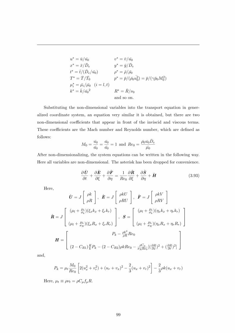
u∗ = u/u0 v∗ = v/u0
x∗ = x/De y∗ = y/De
t∗ = t/(De/u0) ρ∗ = ρ/ρ0
T ∗ = T /T0 p∗ = p/(ρ0u20) = p/(γp0M
20 )
µ∗i = µi/µ0 (i = l, t)
k∗ = k/a02 R∗ = R/ν0
and so on.
Substituting the non-dimensional variables into the transport equation in gener-
alized coordinate system, an equation very similar it is obtained, but there are two
non-dimensional coefficients that appear in front of the inviscid and viscous terms.
These coefficients are the Mach number and Reynolds number, which are defined as
follows:
M0 =u0
a0=a0
a0= 1 and Re0 =
ρ0u0De
µ0
After non-dimensionalizing, the system equations can be written in the following way.
Here all variables are non-dimensional. The asterisk has been dropped for convenience.
∂U
∂t+∂E
∂ξ+∂F
∂η=
1
Re0
∂R
∂ξ+∂S
∂η+ H (3.93)
Here,
U = J
[ρk
ρR
], E = J
[ρkU
ρRU
], F = J
[ρkV
ρRV
]
R = J
(µl + µtσk
)(ξxkx + ξrkr)
(µl + µtσR
)(ξxRx + ξrRr)
, S =
(µl + µtσk
)(ηxkx + ηrkr)
(µl + µtσR
)(ηxRx + ηrRr)
H =
Pk − ρk2
ρRRe0
(2− CR1)Rk Pk − (2− CR2)ρkRe0 − ρCµσRRe0
[(∂R∂x )2 + (∂R∂r )2]
and,
Pk = µtM0
Re0
[2(u2
x + v2r ) + (ur + vx)2 − 2
3(ux + vr)
2
]− 2
3ρk(ux + vr)
Here, µt ≡ ρνt = ρCµfµR.
99
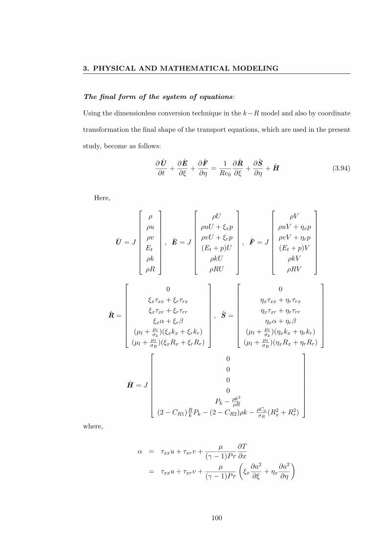
3. PHYSICAL AND MATHEMATICAL MODELING
The final form of the system of equations:
Using the dimensionless conversion technique in the k−R model and also by coordinate
transformation the final shape of the transport equations, which are used in the present
study, become as follows:
∂U
∂t+∂E
∂ξ+∂F
∂η=
1
Re0
∂R
∂ξ+∂S
∂η+ H (3.94)
Here,
U = J
ρ
ρu
ρv
Et
ρk
ρR
, E = J
ρU
ρuU + ξxp
ρvU + ξrp
(Et + p)U
ρkU
ρRU
, F = J
ρV
ρuV + ηxp
ρvV + ηrp
(Et + p)V
ρkV
ρRV
R =
0
ξxτxx + ξrτrx
ξxτxr + ξrτrr
ξxα+ ξrβ
(µl + µtσk
)(ξxkx + ξrkr)
(µl + µtσR
)(ξxRx + ξrRr)
, S =
0
ηxτxx + ηrτrx
ηxτxr + ηrτrr
ηxα+ ηrβ
(µl + µtσk
)(ηxkx + ηrkr)
(µl + µtσR
)(ηxRx + ηrRr)
H = J
0
0
0
0
Pk − ρk2
ρR
(2− CR1)Rk Pk − (2− CR2)ρk − ρCµσR
(R2x +R2
r)
where,
α = τxxu+ τxrv +µ
(γ − 1)Pr
∂T
∂x
= τxxu+ τxrv +µ
(γ − 1)Pr
(ξx∂a2
∂ξ+ ηx
∂a2
∂η
)
100
β = τrxu+ τrrv +µ
(γ − 1)Pr
∂T
∂r
= τrxu+ τrrv +µ
(γ − 1)Pr
(ξr∂a2
∂ξ+ ηr
∂a2
∂η
)The components of stress tensor are as follows:
τxx =2
3µ [2(uξξx + uηηx)− (vξξr + vηηr)]
τxr = µ (uξξr + uηηr) + vξξx + vηηx)
τrr =2
3µ [2(vξξr + vηηr)− (uξξx + uηηx)]
and the viscosity and Prandtl number can be defined as
µ = µl + µt
µ
Pr=
µlPrl
+µtPrt
The turbulence production term Pk is given as follows:
Pk =µtRe0
[2(u2
x + v2r ) + (ur + vx)2 − 2
3(ux + vr)
2
]− 2
3ρk(ux + vr)
The unbalance of the production and dissipation of turbulent kinetic energy k due
to rapid change in the density is occurred at the shock regions, and it’s creates a big
problem in solving such flow features numerically. In solving this problem, Yamamoto
& Daiguji [1991] introduced a limiter function which working at the early stage of the
calculation to suppress the instability.
pk = min[Pk, C2CbρεRe/C1] (3.95)
where Cb(> 1) is a limiting parameter determined by the empirical approach, C1 = 1.44,
and C2 = 1.92[1− exp(−Re2t )].
Here,
fµ =tanh(α′Ret)
tanh(β′Ret)
Ret ≡R
νl=
ρ
µlR
101
3. PHYSICAL AND MATHEMATICAL MODELING
and model constants are:
σk = 1.0, σR = 1.080, CR1 = 1.44, CR2 = 1.92, Cµ = 0.09
α′ = 0.005, β′ =C
3/4µ
2k, where, k2 = σR
√Cµ(CR2 − CR1)
3.3.2.2 Initial and boundary conditions
This two-equation k − R model for turbulence modeling is subjected to the following
boundary conditions [Goldberg, 1994, 1996; Yamamoto & Daiguji, 1991]:
• On solid walls
k = 0, R = 0
• Symmetry surface∂k
∂r= 0,
∂R
∂x= 0
where, r is the normal-to-surface direction.
• Free stream (and initial) condition
k = 1× 10⁻⁶, R = O(10−5) 1
3.4 Conclusion
In this chapter, a detail discussion is made on the fundamental conservation laws,
non-dimensionalizing, and the transformation of governing equations from orthogonal
coordinate system to generalized curvilinear coordinate system. The turbulence model-
ing in consequences Reynolds averaging, eddy-viscosity hypothesis and k−R turbulence
model used in the study are described.
102