Study of a neural network-based system

for stability augmentation of an airplane Author: Roger Isanta Navarro

Annex 1

Introduction to Neural Networks and

Adaptive Neuro-Fuzzy Inference Systems (ANFIS)

Supervisors: Oriol Lizandra Dalmases

Fatiha Nejjari Akhi-Elarab

Aeronautical Engineering

September 2013

This page intentionally left blank

i

Contents

1 Introduction to neural networks ......................................................................... 1

1.1 Main applications of Neural Networks ............................................................... 1

1.2 Advantages and disadvantages of Neural Networks .......................................... 2

1.3 Biological foundations of Neural Networks ........................................................ 3

1.4 The artificial neuron ........................................................................................... 4

1.5 Neural Network typologies................................................................................. 5

2 Required mathematical and numerical tools ........................................................ 7

2.1 Matrix inversion formula .................................................................................... 7

2.2 Least-Squares Method ....................................................................................... 7

2.3 Recursive Least-Squares Method ....................................................................... 8

2.4 Method of Steepest Descent .............................................................................. 9

3 ANFIS Networks ................................................................................................ 12

3.1 Fuzzy logic, fuzzy inference systems and the Sugeno fuzzy model ................... 12

3.2 Advantages of ANFIS over Multilayer Perceptrons (MLP) ................................ 13

3.3 Architecture ..................................................................................................... 14

3.4 ANFIS Hybrid Learning ...................................................................................... 16

3.4.1 Forward pass ............................................................................................ 17

3.4.2 Backward pass .......................................................................................... 17

ii

List of figures

Figure ‎1.1 Main neural elements .................................................................................... 3

Figure ‎1.2 Artificial neuron model .................................................................................. 4

Figure ‎1.3 Examples of step and sigmoidal activation functions .................................... 5

Figure ‎2.1 Generic convergence diagram of total output error with constant step ..... 10

Figure ‎2.2 Generic convergence diagram of total output error with variable step ...... 11

Figure ‎3.1 The Sugeno fuzzy model .............................................................................. 13

Figure ‎3.2 Diagram representation of a 3-inputs 3-rules ANFIS network ..................... 14

1

1 Introduction to neural networks

Artificial Neural Networks are nonlinear mapping systems whose structure is based in

the observed human and animal nervous systems; they are mathematical

approximations to the human brain function. Nevertheless, they are not directly

comparable to the brain, nor are their operation principles, for they do not base

themselves solely in biological networks operation, they only emulate a very simple

portion of human its functions and are not able to simulate the highly complex relational

neurobiological processes that occur within it.

Processing units are named neurons. Artificial Neural Networks (from now on Neural

Networks) comprise a large number of these processing units, each of which receives

weighted input from other units (or nodes) and generates a scalar output depending on

the available local information stored internally and the information arriving through the

incoming weighted connections.

A Neural Network is characterized by the following aspects:

- A set of processing units or neurons.

- An activation state for each unit, equivalent to the output of the unit.

- Connections between units, often defined by a weight that modifies the effect

of the input signal in the unit.

- A propagation rule, which specifies the effective entry of a unit as a function of

the external entries.

- An activation function based on the effective entry and the previous activation.

- An external input corresponding to a term known as bias for each unit.

- A method to gather information, corresponding to the learning rule.

- An environment in which the system is going to operate.

1.1 Main applications of Neural Networks

Applications of Neural Networks are diverse and so are the areas in which they are of

use. The main applications of Neural Networks are those in which the inferring

approximation and use of functions is required via observation or measure, these tasks

classify in following categories:

- Function approximation

- Data classification

- Data processing

- System control

2

System control is the most recent application of Neural Networks and is the field in

which most efforts are invested actually. It is also the field in which is developed this

study.

Specific areas of application of the Neural Networks are also varied, the most significant

follow:

- Automotive and transport: automatic pilot systems, failure detection by external

vibration detection, truck brakes diagnosis, fleet tracking systems.

- Banking and finances: checks and other documents reading, credit applications

and risks evaluation, real properties appraisal, loans assessment, price evolution

forecasting, fake identifications, signature interpretation and identification, use

of credit line analysis.

- Electronics: code sequence prediction, elements distribution in integrated

circuits, process control, failure analysis, artificial vision, voice recognition.

- Manufacturing: production and process control, product analysis and design,

failure diagnosis, automatic visual quality inspection.

- Medicine: EEG and ECG analysis, prosthesis design, optimization of transplant

times, recognition and prediction of infarctions via ECG, reduction of hospital

costs.

- Robotics: dynamic control of trajectory, controllers, optical systems.

- Security: adaptive security codes, cryptography, digital recognition of

fingerprints.

- Telecommunications: data compression, automation of information services,

real time translation of spoken language.

- Voice: voice recognition, voice comprehension, vowel classification,

transformation from text to voice.

1.2 Advantages and disadvantages of Neural Networks

Neural Networks present several advantages over other processing systems, the most

significant being:

- Neural Networks can synthesize algorithms through a learning process.

- To use neural technology it is not necessary to now the mathematical details. It

is only required familiarity with the job data.

- The solution of nonlinear problems is one of the strengths of the Neural

Networks.

- Neural Networks are robust. They might fail in some processing elements, but

the network keeps on working, as opposed as in traditional programming.

3

However, some disadvantages are also characteristic of Neural Networks:

- Neural Networks must be trained for each problem. Moreover, multiple tests

must be conducted to define the adequate architecture. Training might be long

and CPU time consuming.

- The training requirement involves large volumes of data.

Neural Networks present a complex issue for external observers who would want to

make modifications in it. To add new knowledge is necessary to change the interactions

of many units so that its unified effect might synthesize this new knowledge.

1.3 Biological foundations of Neural Networks

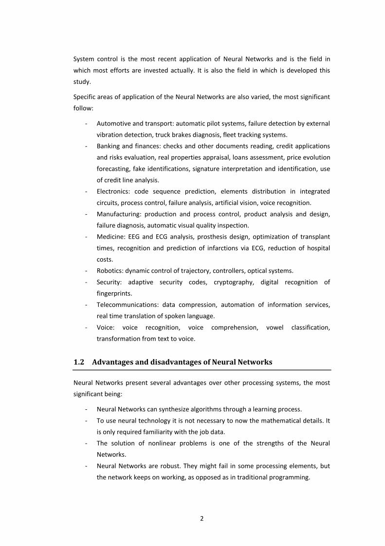
A biological neuron is a cell specialized in information processing. It divides, from a

simplified point of view, into the cell body (soma) and two different kinds of

ramifications: dendrites and the axon; the firsts drive pulse inputs to the soma and the

later transmits the output signals generated by the body of the cell.

Figure ‎1.1 Main neural elements

The signals that reach the neuron through the dendrites are weighted by a parameter

called weight, associated to the corresponding synapsis. These weights might excite the

neuron (positive weight synapsis) or inhibit it (negative weight synapsis).

The soma then integrates and combines the different weighted input signals, and emits

an output signal depending on the sum of the weighted entries: if the sum is higher or

equal to the activation threshold of the neuron, the output is generated and sent

through the axon.

4

The ability to adjust the signals, by modifying the weight values, results in a learning

mechanism which is the training methodology of the artificial neural networks.

1.4 The artificial neuron

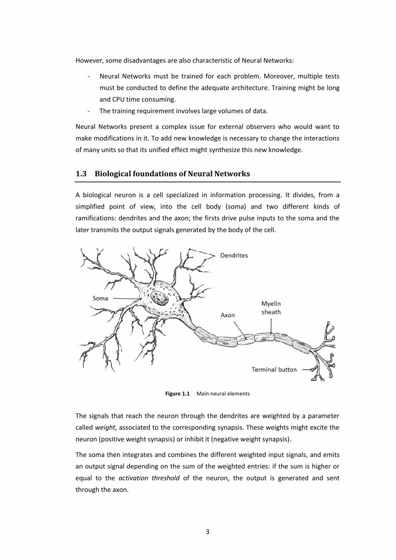
As stated, an artificial neuron is a mathematical approximation to the biological neuron

function. Within the generic artificial neuron two processes occur: the first one is the

algebraic sum of the inputs of synapsis and the second is the evaluation of a nonlinear

function resulting in its output value.

Figure ‎1.2 Artificial neuron model

The algebraic sum that will be lately evaluated by the nonlinear function can be written

as a function of the synaptic weights , entry signals and a bias .

( ) ∑ ( ) ( )

(‎1.1)

where counts the total of incoming connections.

The polarization or threshold of the neuron is an external parameter, however it can be

considered as additional entry :

( ) ( ) ( ) ∑ ( ) ( )

( ) (‎1.2)

is called the activation potential.

The neuron output, results from the evaluation of the activation function , which takes

the activation potential as argument and may also take the previous output.

( ) ( ( ) ( )) (‎1.3)

5

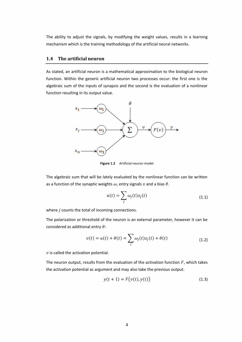
If the previous output is not considered as argument, the resulting value of the whole

process of integration and evaluation within the neuron can be written as

( ) (∑ ( ) ( )

( )) (‎1.4)

Many activation functions are used as step, linear, hyperbolic tangent or sigmoidal

functions among others.

Figure ‎1.3 Examples of step and sigmoidal activation functions

1.5 Neural Network typologies

Artificial Neural Networks may be classified differentiating between neuron function,

single or multilayered networks, training methodologies, whether the flow of

information is recurrent or feed-forward, etc.

McCulloch and Pits, in 1943, introduced the simple artificial neuron. These are neurons

which accept values of zero or one as incoming signals and present an activation

threshold of one or two, thus allowing the implementation of a logic OR (in case of one

as activation threshold) or a logic AND (in case of the activation threshold being equal to

two). The integration of postsynaptic pulses is lineal in this kind of neurons.

In more realistic neuron designs the entry signals may be a real value and are subject to

varying weights.

Different neuron models have been designed to fulfill specific requirements such the use

of integration methods other than simple algebraic addition in which the entry signals

are defined as functions of time ( ) which describe changes in time on the

voltage ( ). Other neurons such as the ones used within the ANFIS network proposed

in this study have special functions such as the product of all their entries, a quotient or

the computation of a function linear or nonlinear to some defined or varying

parameters.

-0.5

0

0.5

1

1.5

y

u

-1.5

-1

-0.5

0

0.5

1

1.5

y

u

6

Neural networks may also be differentiated after their number of layers. Simplest layers

have only one or two layers, the second usually being a sum of the previous node

outputs, an example of such neural networks are Simple Perceptrons, whose goal is

usually the division of an n-dimensional space into two sub spaces according to a

criterion. A neural network differentiating between whether a color is dark or light may

be achieved through the implementation of a Simple Single Layered Perceptron. The

frontier of decision, which is equivalent to the reaching of the activation threshold in the

neuron, may be defined by one of many activation functions of which some have been

mentioned earlier.

To solve more complicated problems multilayered networks are usually required. There

is a great variety of such networks for they allow considerable specialization on the

problem at hand. The two most common multilayered neural networks being the

Multilayered Perceptron, an extension of the Simple Perceptron to a multilayer scheme,

and the Adaptive Neuro-Fuzzy Inference System (ANFIS) network, which is the one used

within this study.

The structure of the network and the subsequent flow of information are also significant

differences between networks, thus the so-called Feed-Forward networks are those in

which the information flows from a layer to a strictly superior layer for all layers and

nodes of the network. On the contrary, a recurrent network will be that in which one or

more nodes receive as input the output of another node in a subsequent layer.

Training methodologies are also a significant distinguishing characteristic and are

intrinsically related to the network structure. The linearity or nonlinearity to the global

network output of some of the its varying parameters will allow or prevent the use of

optimization methods like the Least Squares Method presented in subsections ‎2.2

and ‎2.3 and the nonlinearity or a recurrent structure will require the use of other

optimization procedures such as derivative-based methods as the Steepest Descent

presented in subsection ‎2.4 or derivative-free methods such as Genetic Algorithms.

7

2 Required mathematical and numerical tools

Within this section the main mathematical and numerical tools that will later be used to

develop the neural network training will be presented.

2.1 Matrix inversion formula

The matrix inversion formula will be of importance in the following Recursive Least-

Squares Method subsection.

This formula states that given two nonsingular square matrices and , then

( ) ( ) (‎2.1)

Proof of this statement can be found in [2].

2.2 Least-Squares Method

Least-Squares Method is a standard method to compute the set of parameters that will

best approximate the solution to an overdetermined system. To do so, the sum of the

squares of the errors is minimized.

Consider a linear system of equations consisting in equations and unknown

parameters

(‎2.2)

where is an matrix, is the unknown parameter vector and is the

solution vector. It is obvious that if , the matrix will be squared and the

exact solution to the system, provided that is nonsingular, can be easily calculated by

(‎2.3)

If , which is a very common situation in neural network training, as well as in

many other applications, an exact solution is not always possible, either because the

model is not appropriate enough to describe the system, or because of the existence of

noise or error contamination in the data. Equation (‎2.2) should be modified to account

for this error:

(‎2.4)

As defined previously, the main goal of the method is finding an approximate vector

which minimizes the sum of squared error.

8

∑( )

( ) ( ) (‎2.5)

where is the ith row of . The expression in the previous equation may be expanded,

derived and equated to as follows:

(‎2.6)

( )

(‎2.7)

At , ( )

(‎2.8)

If is non-singular, can be solved:

( ) (‎2.9)

2.3 Recursive Least-Squares Method

One important drawback of the previously disclosed Least-Squares Method resides in

the necessity of inverting the matrix: an operation requiring a high computational

cost if is not small enough. Moreover, the Least-Squares Method, as presented

previously, does not take advantage of the recently computed values, but given

additional equations to the system, requires the total recalculation of the method. The

following procedure presents a recursive method to account for an additional equation

in the system, that is, an extra training pair ( ), taking in consideration the previous

values.

From now on, the circumflex symbol denoting the approximate solution will be

omitted for simplicity.

Considering the unknown parameter vector at step

( ) (‎2.10)

the same vector at step can be written as:

([

]

[ ])

[ ]

[ ]

(‎2.11)

The following and are introduced

( ) (‎2.12)

9

([

]

[ ])

( ) (‎2.13)

Using the matrix inversion formula presented at the beginning of this section, the

computation of can be rewritten as an incremental formula:

(

)

(‎2.14)

Once known , an incremental expression for can easily be found.

( ) (‎2.15)

can be eliminated from this expression using the Equation (‎2.10)

(‎2.16)

( ) [(

) ] (‎2.17)

yielding the final incremental expression for :

( ) (‎2.18)

The sequential calculation of given , using Recursive Least-Squares Method can

be summarized in the following two steps:

{

( )

(‎2.19)

where the initial equals ( ) .

2.4 Method of Steepest Descent

Descent methods main goal is also the minimization of a function defined on an -

dimensional input space [ ] . The objective function might not have

linear form with respect to , as opposed as considered in the Least-Squares Method

(variations of Least-Squares Method exist for nonlinear models, however these will not

be considered since will not be used within this study). Also as opposed to the Least-

Squares Method, this local minimum is found iteratively due to the complexity and non-

linearity of .

Within one iteration, the next values vector, denoted by , is computed by a step

from of size in a direction so that ( ) ( )

10

(‎2.20)

( ) ( ) ( ) (‎2.21)

The computation of step is performed through two procedures: determination of

direction and determination of the step size . Many different methods exist whose

main difference lies in the computation of the first procedure, while the step size is

commonly determined by line minimization. However, some methods do not use line

minimization, which is the case of the two methods presented below.

The taken corresponds to the direction in which decreases more quickly, that is

( ).

( ) (‎2.22)

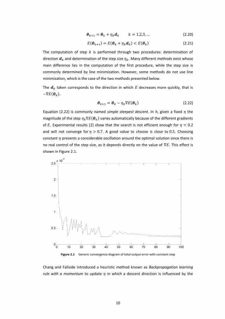
Equation (‎2.22) is commonly named simple steepest descent. In it, given a fixed the

magnitude of the step ( ) varies automatically because of the different gradients

of . Experimental results [2] show that the search is not efficient enough for

and will not converge for . A good value to choose is close to . Choosing

constant presents a considerable oscillation around the optimal solution since there is

no real control of the step size, as it depends directly on the value of . This effect is

shown in Figure ‎2.1.

Figure ‎2.1 Generic convergence diagram of total output error with constant step

Chang and Fallside introduced a heuristic method known as Backpropagation learning

rule with a momentum to update in which a descent direction is influenced by the

11

previous one, and the step size increases when the direction “looks good” according to

the relation between both directions [2].

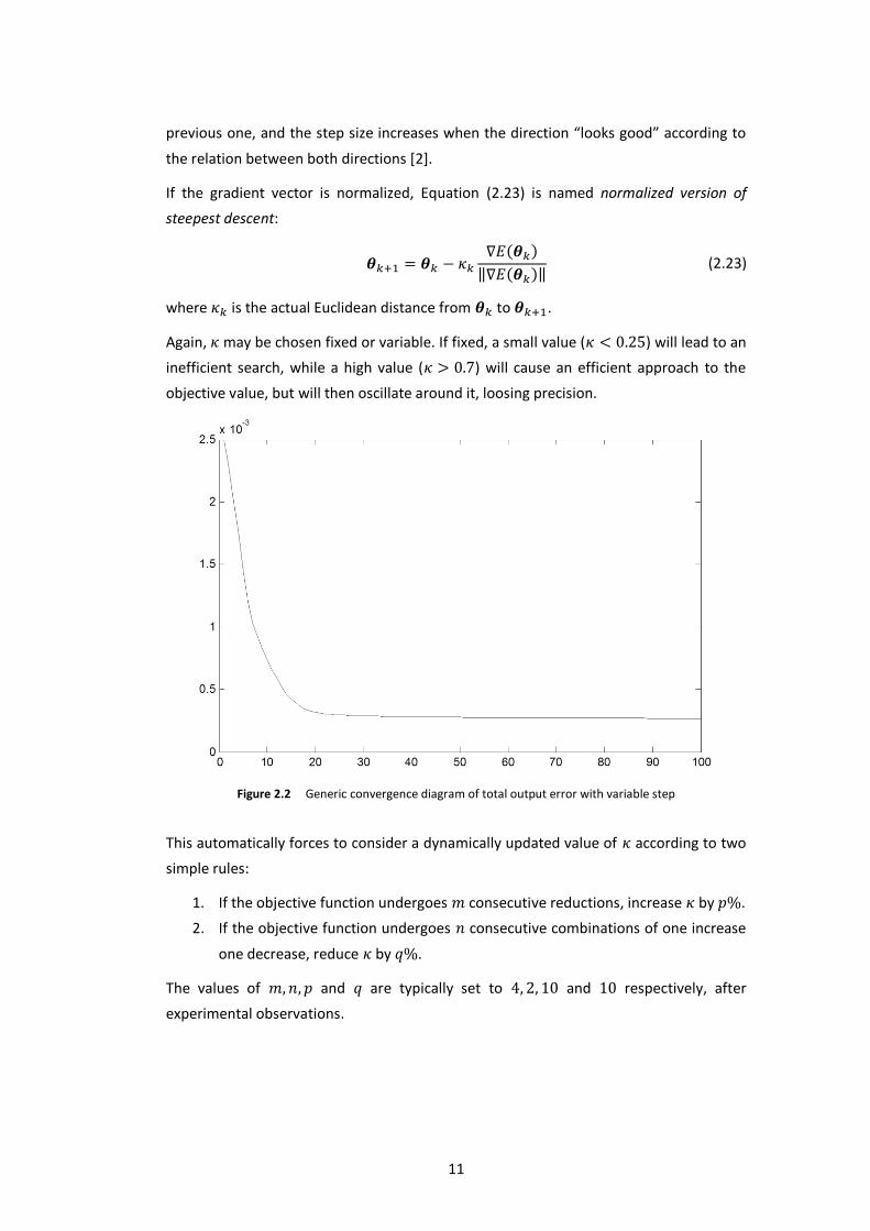
If the gradient vector is normalized, Equation (‎2.23) is named normalized version of

steepest descent:

( )

‖ ( )‖ (‎2.23)

where is the actual Euclidean distance from to .

Again, may be chosen fixed or variable. If fixed, a small value ( ) will lead to an

inefficient search, while a high value ( ) will cause an efficient approach to the

objective value, but will then oscillate around it, loosing precision.

Figure ‎2.2 Generic convergence diagram of total output error with variable step

This automatically forces to consider a dynamically updated value of according to two

simple rules:

1. If the objective function undergoes consecutive reductions, increase by .

2. If the objective function undergoes consecutive combinations of one increase

one decrease, reduce by .

The values of and are typically set to and respectively, after

experimental observations.

12

3 ANFIS Networks

Adaptive Neuro-Fuzzy Inference Systems (ANFIS) are a class of adaptive neural networks

that are functionally equivalent to fuzzy inference systems (described in the following

subsection) and offer the combination of learning, adaptability and nonlinear, time-

variant problem solving characteristics of Artificial Neural Networks plus the important

concepts of approximate reasoning and treatment of information provided by the fuzzy

set theory.

ANFIS network control systems (or neuro-fuzzy systems) represent a hybrid platform for

solving actual complex problems that require the use of intelligent systems and are a

viable alternative to the conventional model-based control schemes. They allow dealing

effectively with the common issues of uncertainty and unknown variations in plant

parameters and structure, hence improving robustness of the control system.

3.1 Fuzzy logic, fuzzy inference systems and the Sugeno fuzzy model

Fuzzy logic [2] is a set of mathematical principles based on degrees of membership to

pre-established functions whose main goal is information modeling; it is a flexible tool

based on linguistic rules dictated by an expert. Fuzzy logic was developed to emulate

human logic and attain correct solutions in spite of the ambiguity of information. In

contrast with conventional logic where strict boundaries are set between the

membership of a variable to a set or another, fuzzy logic presents membership ranks

within the interval between the two sets, and offers a solution based on this dual or

higher membership.

As a simple example, the speed of a car may be classified as high or low for a given

circumstance, and the reaction of the driver when breaking will depend, among other

things, on whether he assigns his current speed to a set or another, or an intermediate

state between them. On one hand, conventional logic will establish strict boundaries

between the proposed sets; for example, driving at less than will be

considered slow and doing so at or more will be considered high speed. Clearly a

problem arises when driving at speeds around , since the response of the driver

subject to conventional logic will vary abruptly when crossing this boundary. On the

other hand, a driver subject to fuzzy logic reasoning will be able to assign partial

memberships to both functions, that is, considering partially high and partially

slow, and provide a much more accurate response. Moreover, if the parameters defining

the membership functions are variable, the fuzzy system will be able, provided a correct

training algorithm, to modify such functions to offer a better response.

13

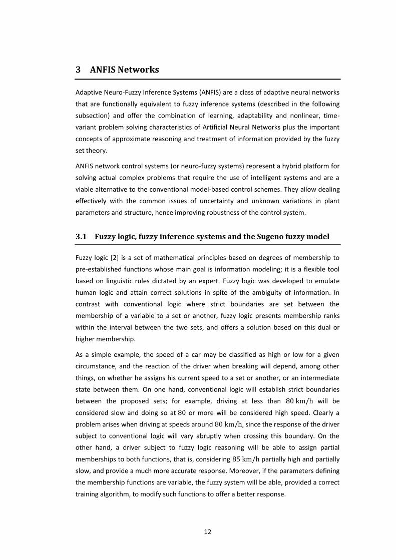
The Sugeno fuzzy model aims to generate a systematic approach towards generating

fuzzy rules from a given input-output data set. Sugeno fuzzy rules are of the form:

( ) (‎3.1)

where and are fuzzy sets and ( ) is a function associated to the fact of

and pertaining to and respectively. ( ) will usually be a polynomial, in what

is then called the first-order Sugeno fuzzy model, in contrast with the zero-order Sugeno

fuzzy model if ( ) were constant.

Figure ‎3.1 shows the fuzzy reasoning procedure for a first-order Sugeno fuzzy model:

Figure ‎3.1 The Sugeno fuzzy model

3.2 Advantages of ANFIS over Multilayer Perceptrons (MLP)

In addition to the general advantages and disadvantages of the Neural Networks, ANFIS

networks present interesting advantages over Multilayer Perceptrons (MLP), which are

the most direct competitors in neural computing for the type of problem treated within

this study. These advantages result from the fact that ANFIS presents a much more

specific mathematical structure which enables it as a good universal adaptive

approximator. The most significant advantages of ANFIS in front of MLPs follow:

1. ANFIS presents a much better learning ability: for a similar network complexity,

a much smaller convergence error is achieved, and although the convergence is

slower the smallness of the error in ANFIS is able to compensate that fact.

2. MLP often present a sudden convergence preceded by a region of considerable

instability.

3. ANFIS can achieve highly nonlinear mapping, far superior to MPL and other

common linear methods of similar complexity.

14

4. ANFIS requires fewer adjustable parameters than those required in other Neural

Network structures and, specifically, backpropagation MPLs.

5. The ANFIS structure allows for parallel computation.

Finally, ANFIS presents two advantages exclusive to its method:

6. ANFIS networks present a well-structured knowledge representation.

7. ANFIS networks allow a better integration with other control design methods.

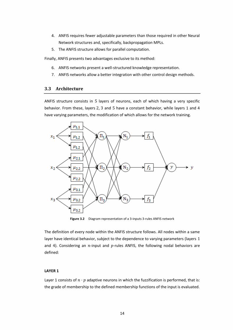
3.3 Architecture

ANFIS structure consists in layers of neurons, each of which having a very specific

behavior. From these, layers , and have a constant behavior, while layers 1 and 4

have varying parameters, the modification of which allows for the network training.

Figure ‎3.2 Diagram representation of a 3-inputs 3-rules ANFIS network

The definition of every node within the ANFIS structure follows. All nodes within a same

layer have identical behavior, subject to the dependence to varying parameters (layers

and ). Considering an -input and -rules ANFIS, the following nodal behaviors are

defined:

LAYER 1

Layer 1 consists of adaptive neurons in which the fuzzification is performed, that is:

the grade of membership to the defined membership functions of the input is evaluated.

15

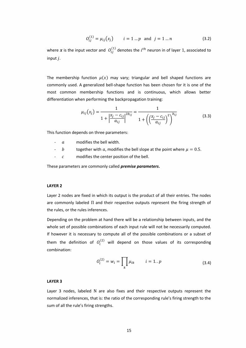
( ) ( ) (‎3.2)

where is the input vector and ( )

denotes the neuron in of layer , associated to

input .

The membership function ( ) may vary; triangular and bell shaped functions are

commonly used. A generalized bell-shape function has been chosen for it is one of the

most common membership functions and is continuous, which allows better

differentiation when performing the backpropagation training:

( )

|

|

((

)

)

(‎3.3)

This function depends on three parameters:

- modifies the bell width.

- together with , modifies the bell slope at the point where .

- modifies the center position of the bell.

These parameters are commonly called premise parameters.

LAYER 2

Layer 2 nodes are fixed in which its output is the product of all their entries. The nodes

are commonly labeled and their respective outputs represent the firing strength of

the rules, or the rules inferences.

Depending on the problem at hand there will be a relationship between inputs, and the

whole set of possible combinations of each input rule will not be necessarily computed.

If however it is necessary to compute all of the possible combinations or a subset of

them the definition of ( )

will depend on those values of its corresponding

combination:

( ) ∏

(‎3.4)

LAYER 3

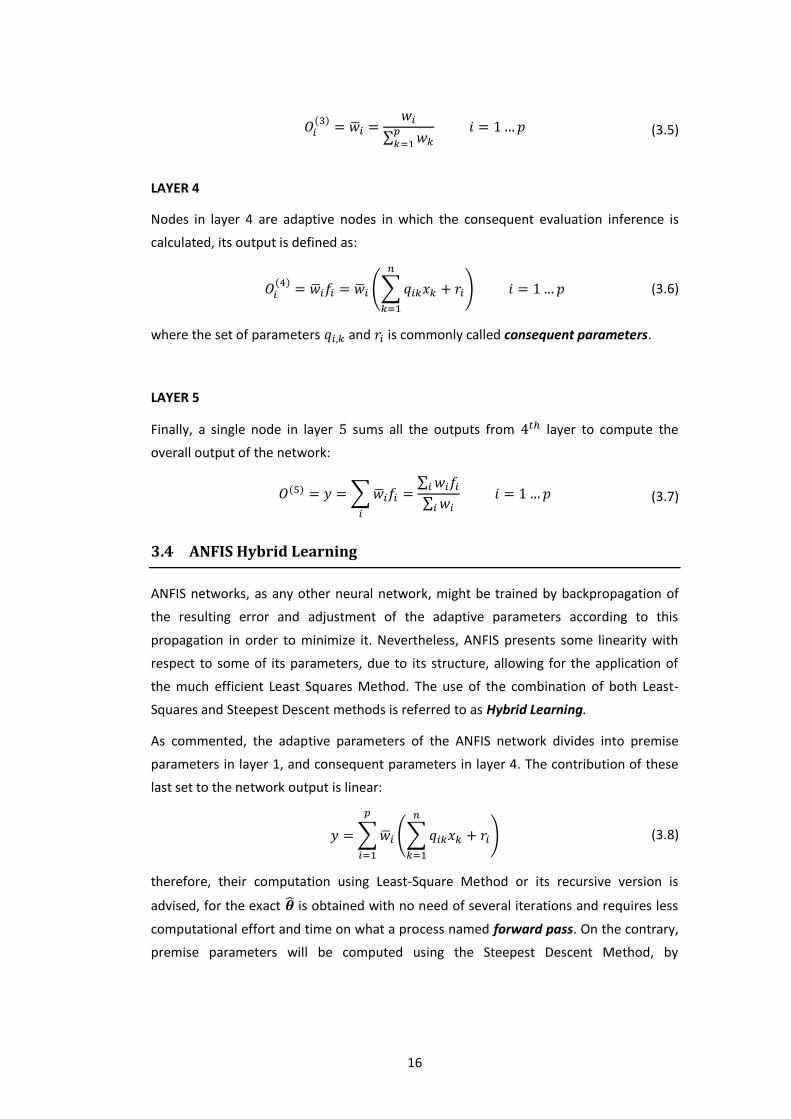
Layer 3 nodes, labeled are also fixes and their respective outputs represent the

normalized inferences, that is: the ratio of the corresponding rule’s firing strength to the

sum of all the rule’s firing strengths.

16

( )

∑

(‎3.5)

LAYER 4

Nodes in layer 4 are adaptive nodes in which the consequent evaluation inference is

calculated, its output is defined as:

( ) (∑

) (‎3.6)

where the set of parameters and is commonly called consequent parameters.

LAYER 5

Finally, a single node in layer sums all the outputs from layer to compute the

overall output of the network:

( ) ∑

∑

∑ (‎3.7)

3.4 ANFIS Hybrid Learning

ANFIS networks, as any other neural network, might be trained by backpropagation of

the resulting error and adjustment of the adaptive parameters according to this

propagation in order to minimize it. Nevertheless, ANFIS presents some linearity with

respect to some of its parameters, due to its structure, allowing for the application of

the much efficient Least Squares Method. The use of the combination of both Least-

Squares and Steepest Descent methods is referred to as Hybrid Learning.

As commented, the adaptive parameters of the ANFIS network divides into premise

parameters in layer 1, and consequent parameters in layer 4. The contribution of these

last set to the network output is linear:

∑ (∑

)

(‎3.8)

therefore, their computation using Least-Square Method or its recursive version is

advised, for the exact is obtained with no need of several iterations and requires less

computational effort and time on what a process named forward pass. On the contrary,

premise parameters will be computed using the Steepest Descent Method, by

17

backpropagating the error through the network, during the backward pass. Both

training steps constitute the Hybrid Learning methodology and are presented below.

3.4.1 Forward pass

In the forward pass the Recursive Least-Square Method is used to evaluate the

consequent parameters. Considering the notation in subsections ‎2.2 and ‎2.3 and a -

input network as the one shown in Figure ‎3.2, the vector will be defined as follows:

{ } (‎3.9)

and will be the desired output vector (not to be confused with the network results,

after Layer 5). Considering that the required number of training pairs to have a definite

system will be ( ), where it is recalled refers to the number of inputs and to

the number of rules, the vector would be as follows:

{ ( )} (‎3.10)

Meanwhile, matrix can be defined after Equations (‎3.6) and (‎3.7):

[

( )

( )

( )

( )

( )

( )

( )

( )

( )

( )

( )

( )

( )

( )

( )

( )

( )

( )

]

(‎3.11)

where the superscript between parenthesis denotes the training pair number and has

been defined ( ) to simplify the notation.

Within the recursive part of the method, the vector corresponding to the training

pair is defined as any row of the matrix :

{ ( )

( ) ( )

( ) ( )

( ) } (‎3.12)

3.4.2 Backward pass

In the backward pass the error signal propagates backwards through the network until

the dependence of this error to each of the premise parameters is evaluated. Once

known this gradient, the parameters may be updated by Steepest Descent:

( ) ( )

‖ ‖ (‎3.13)

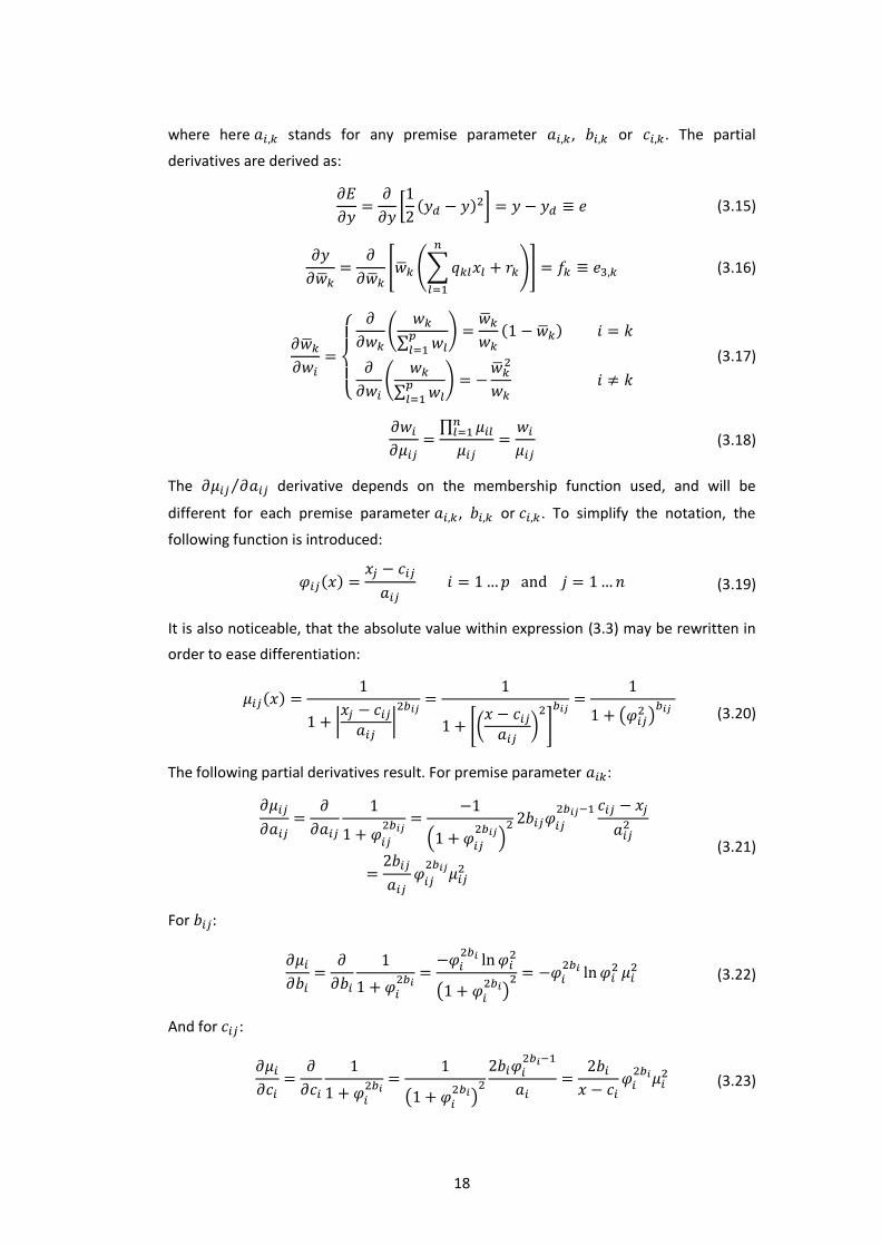
Chain rule is used to evaluate the partial derivatives:

∑

∑

(‎3.14)

18

where here stands for any premise parameter , or . The partial

derivatives are derived as:

[

( )

] (‎3.15)

[ (∑

)] (‎3.16)

{

(

∑

) ( )

(

∑

)

(‎3.17)

∏

(‎3.18)

The ⁄ derivative depends on the membership function used, and will be

different for each premise parameter , or . To simplify the notation, the

following function is introduced:

( )

(‎3.19)

It is also noticeable, that the absolute value within expression (‎3.3) may be rewritten in

order to ease differentiation:

( )

|

|

[(

)

]

( )

(‎3.20)

The following partial derivatives result. For premise parameter :

(

)

(‎3.21)

For :

( )

(‎3.22)

And for :

( )

(‎3.23)

This page intentionally left blank