structur e very helpfull
TRANSCRIPT
1
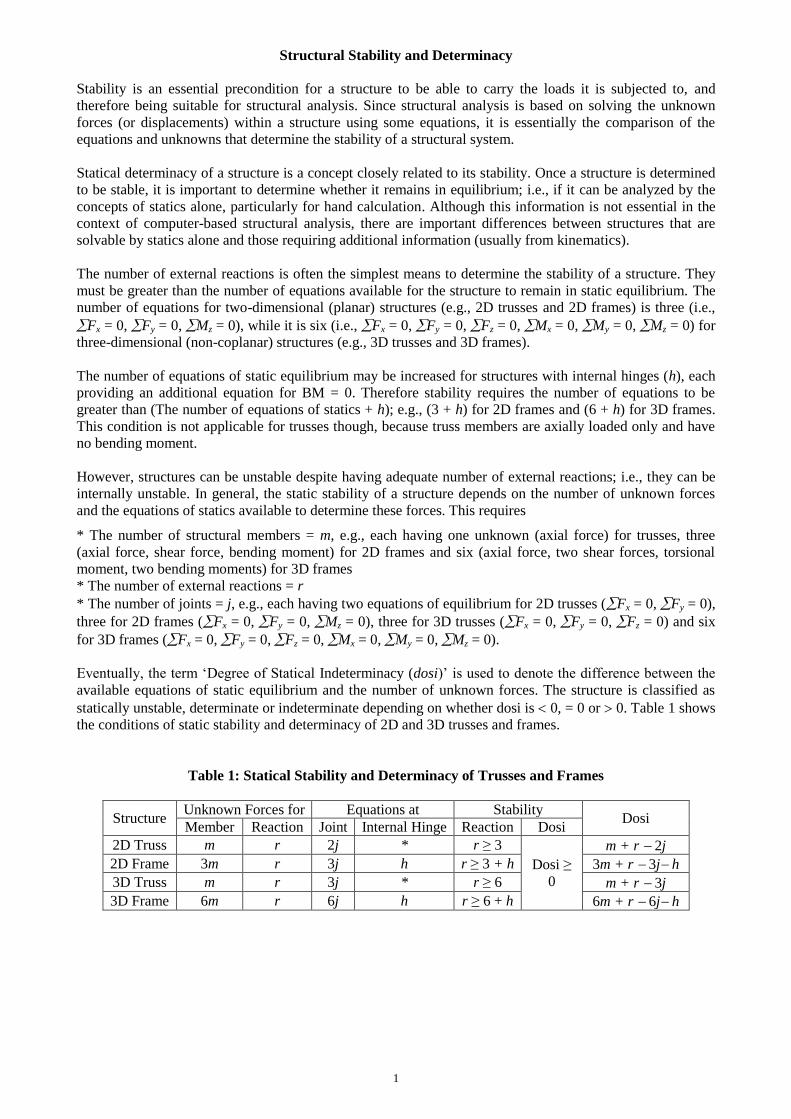
Structural Stability and Determinacy
Stability is an essential precondition for a structure to be able to carry the loads it is subjected to, and
therefore being suitable for structural analysis. Since structural analysis is based on solving the unknown
forces (or displacements) within a structure using some equations, it is essentially the comparison of the
equations and unknowns that determine the stability of a structural system.
Statical determinacy of a structure is a concept closely related to its stability. Once a structure is determined
to be stable, it is important to determine whether it remains in equilibrium; i.e., if it can be analyzed by the
concepts of statics alone, particularly for hand calculation. Although this information is not essential in the
context of computer-based structural analysis, there are important differences between structures that are
solvable by statics alone and those requiring additional information (usually from kinematics).
The number of external reactions is often the simplest means to determine the stability of a structure. They
must be greater than the number of equations available for the structure to remain in static equilibrium. The
number of equations for two-dimensional (planar) structures (e.g., 2D trusses and 2D frames) is three (i.e.,
Fx = 0, Fy = 0, Mz = 0), while it is six (i.e., Fx = 0, Fy = 0, Fz = 0, Mx = 0, My = 0, Mz = 0) for
three-dimensional (non-coplanar) structures (e.g., 3D trusses and 3D frames).
The number of equations of static equilibrium may be increased for structures with internal hinges (h), each
providing an additional equation for BM = 0. Therefore stability requires the number of equations to be
greater than (The number of equations of statics + h); e.g., (3 + h) for 2D frames and (6 + h) for 3D frames.
This condition is not applicable for trusses though, because truss members are axially loaded only and have
no bending moment.
However, structures can be unstable despite having adequate number of external reactions; i.e., they can be
internally unstable. In general, the static stability of a structure depends on the number of unknown forces
and the equations of statics available to determine these forces. This requires
* The number of structural members = m, e.g., each having one unknown (axial force) for trusses, three
(axial force, shear force, bending moment) for 2D frames and six (axial force, two shear forces, torsional
moment, two bending moments) for 3D frames
* The number of external reactions = r
* The number of joints = j, e.g., each having two equations of equilibrium for 2D trusses (Fx = 0, Fy = 0),
three for 2D frames (Fx = 0, Fy = 0, Mz = 0), three for 3D trusses (Fx = 0, Fy = 0, Fz = 0) and six
for 3D frames (Fx = 0, Fy = 0, Fz = 0, Mx = 0, My = 0, Mz = 0).
Eventually, the term ‘Degree of Statical Indeterminacy (dosi)’ is used to denote the difference between the
available equations of static equilibrium and the number of unknown forces. The structure is classified as
statically unstable, determinate or indeterminate depending on whether dosi is 0, = 0 or 0. Table 1 shows
the conditions of static stability and determinacy of 2D and 3D trusses and frames.
Table 1: Statical Stability and Determinacy of Trusses and Frames
Structure Unknown Forces for Equations at Stability
Dosi Member Reaction Joint Internal Hinge Reaction Dosi
2D Truss m r 2j * r ≥ 3
Dosi ≥
0
m + r 2j
2D Frame 3m r 3j h r ≥ 3 + h 3m + r 3j h
3D Truss m r 3j * r ≥ 6 m + r 3j
3D Frame 6m r 6j h r ≥ 6 + h 6m + r 6j h
2
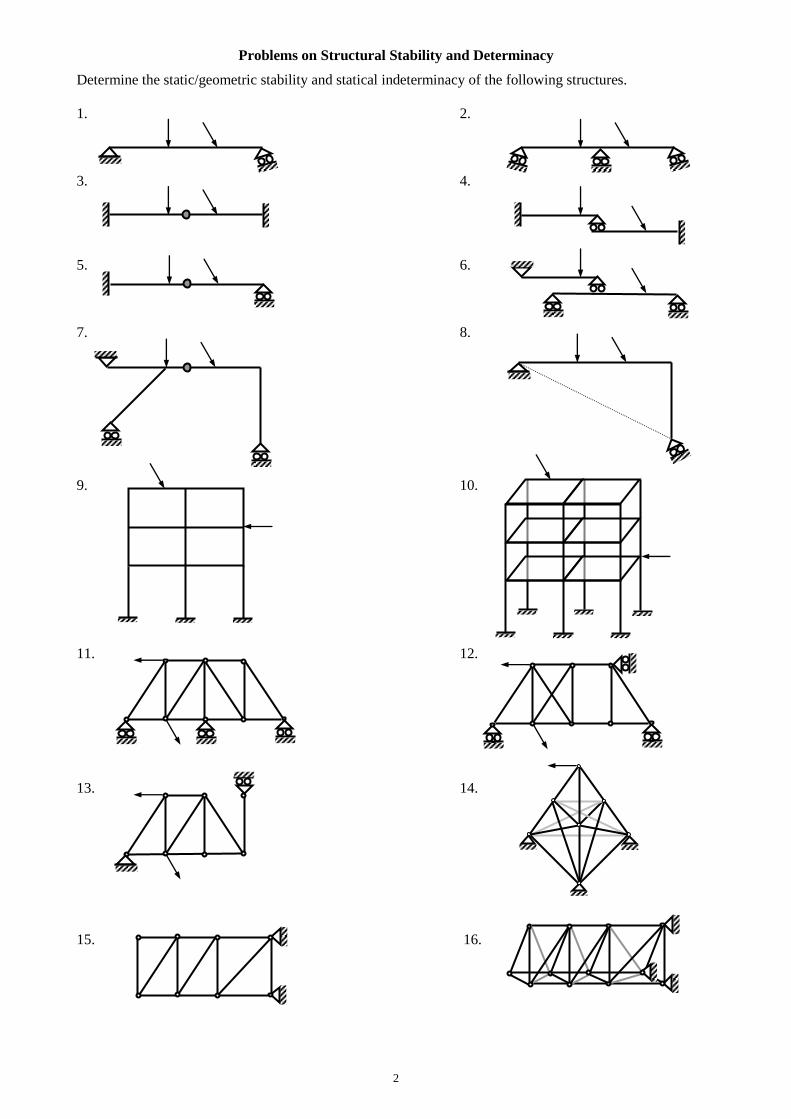
Problems on Structural Stability and Determinacy
Determine the static/geometric stability and statical indeterminacy of the following structures.
1. 2.
3. 4.
5. 6.
7. 8.
9. 10.
11. 12.
13. 14.
15. 16.
3
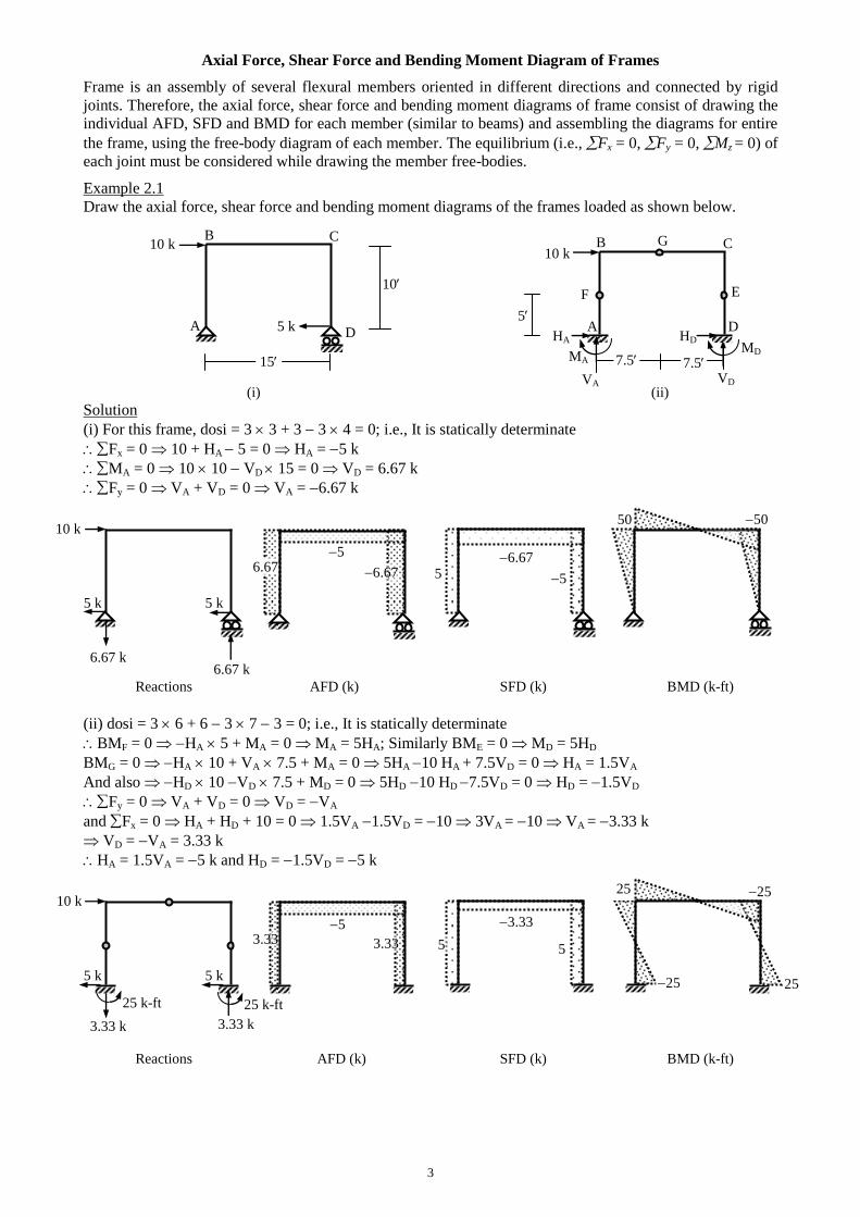
Axial Force, Shear Force and Bending Moment Diagram of Frames
Frame is an assembly of several flexural members oriented in different directions and connected by rigid
joints. Therefore, the axial force, shear force and bending moment diagrams of frame consist of drawing the
individual AFD, SFD and BMD for each member (similar to beams) and assembling the diagrams for entire
the frame, using the free-body diagram of each member. The equilibrium (i.e., Fx = 0, Fy = 0, Mz = 0) of
each joint must be considered while drawing the member free-bodies.
Example 2.1
Draw the axial force, shear force and bending moment diagrams of the frames loaded as shown below.
(i) (ii) Solution
(i) For this frame, dosi = 3 3 + 3 3 4 = 0; i.e., It is statically determinate
Fx = 0 10 + HA 5 = 0 HA = 5 k
MA = 0 10 10 VD 15 = 0 VD = 6.67 k
Fy = 0 VA + VD = 0 VA = 6.67 k
Reactions AFD (k) SFD (k) BMD (k-ft)
(ii) dosi = 3 6 + 6 3 7 3 = 0; i.e., It is statically determinate
BMF = 0 HA 5 + MA = 0 MA = 5HA; Similarly BME = 0 MD = 5HD
BMG = 0 HA 10 + VA 7.5 + MA = 0 5HA 10 HA + 7.5VD = 0 HA = 1.5VA
And also HD 10 VD 7.5 + MD = 0 5HD 10 HD 7.5VD = 0 HD = 1.5VD
Fy = 0 VA + VD = 0 VD = VA
and Fx = 0 HA + HD + 10 = 0 1.5VA 1.5VD = 10 3VA = 10 VA = 3.33 k
VD = VA = 3.33 k
HA = 1.5VA = 5 k and HD = 1.5VD = 5 k
Reactions AFD (k) SFD (k) BMD (k-ft)
5
10 k
25 k-ft
6.67 k 6.67 k
5 k 5 k
10 k
6.67 6.67 5 5
6.67
50 50
D A
25 k-ft
3.33 k 3.33 k
5 k 5 k
3.33 3.33
5
5 5
3.33
25 25
25 25
MD
VD
HD
G C B 10 k
7.5 7.5
E F
5
MA
VA
HA D
C B
A
10 k
15
10
5 k
4
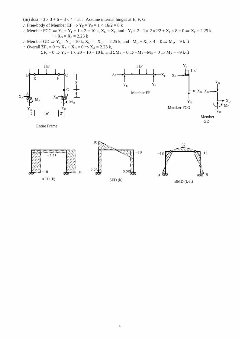
(iii) dosi = 3 3 + 6 3 4 = 3; Assume internal hinges at E, F, G
Free-body of Member EF YE = YF = 1 16/2 = 8 k
Member FCG YG = YF + 1 2 = 10 k, XG = XF, and YF 2 1 2 2/2 + XF 8 = 0 XF = 2.25 k
XG = XF = 2.25 k
Member GD YD = YG = 10 k, XD = XG = 2.25 k, and MD + XG 4 = 0 MD = 9 k-ft
Overall Fx = 0 XA + XD = 0 XA = 2.25 k,
Fy = 0 YA = 1 20 10 = 10 k, and MA = 0 MA MD = 0 MA = 9 k-ft
Member EF
Member FCG
Member
GD
Entire Frame
−10
2.25
MA
YD
YA
XA
MD
1 k/′
D
B
A G
E F
YE YF
XE XF
2′ 2′ 16′
1 k/′
XF
YF
XG
YG
YD
XG
YG
XD MD
4′
1 k/′
XD
SFD (k)
10
−2.25
C
8′
−18
9 −10
−18
9
32
BMD (k-ft) AFD (k)
−10
−2.25
5
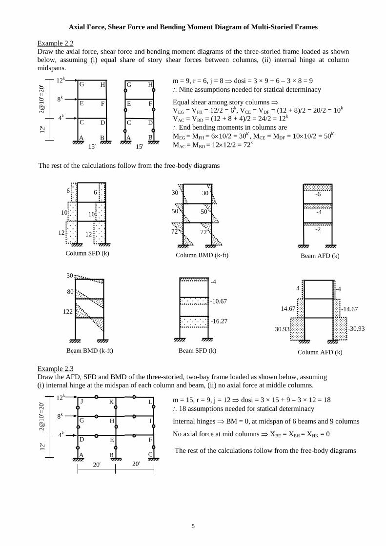
Axial Force, Shear Force and Bending Moment Diagram of Multi-Storied Frames
Example 2.2
Draw the axial force, shear force and bending moment diagrams of the three-storied frame loaded as shown
below, assuming (i) equal share of story shear forces between columns, (ii) internal hinge at column
midspans.
Example 2.3
Draw the AFD, SFD and BMD of the three-storied, two-bay frame loaded as shown below, assuming
(i) internal hinge at the midspan of each column and beam, (ii) no axial force at middle columns.
-4
C
A
80
30
15
15
12k
8k
4k
12
2@
10=
20
Column SFD (k)
Beam BMD (k-ft) Beam SFD (k) Column AFD (k)
122
-10.67
-4
4
30.93
-14.67
-16.27
12
10
6
m = 9, r = 6, j = 8 dosi = 3 × 9 + 6 3 × 8 = 9
Nine assumptions needed for statical determinacy
Equal shear among story columns
VEG = VFH = 12/2 = 6k, VCE = VDF = (12 + 8)/2 = 20/2 = 10
k
VAC = VBD = (12 + 8 + 4)/2 = 24/2 = 12k
End bending moments in columns are
MEG = MFH = 610/2 = 30k, MCE = MDF = 1010/2 = 50
k
MAC = MBD = 1212/2 = 72k
G
E
D
B
H
F
C
A
G
E
D
H
F
B
The rest of the calculations follow from the free-body diagrams
Column BMD (k-ft)
72
50
30
72
50
30
Beam AFD (k)
-6
-4
-2
-30.93
14.67
12
10
6
D
A
20
20
12k
8k
4k
12
2@
10=
20 m = 15, r = 9, j = 12 dosi = 3 × 15 + 9 3 × 12 = 18
18 assumptions needed for statical determinacy
Internal hinges BM = 0, at midspan of 6 beams and 9 columns
No axial force at mid columns XBE = XEH = XHK = 0
J
G
E
B
K
H
F
L
I
C The rest of the calculations follow from the free-body diagrams
6
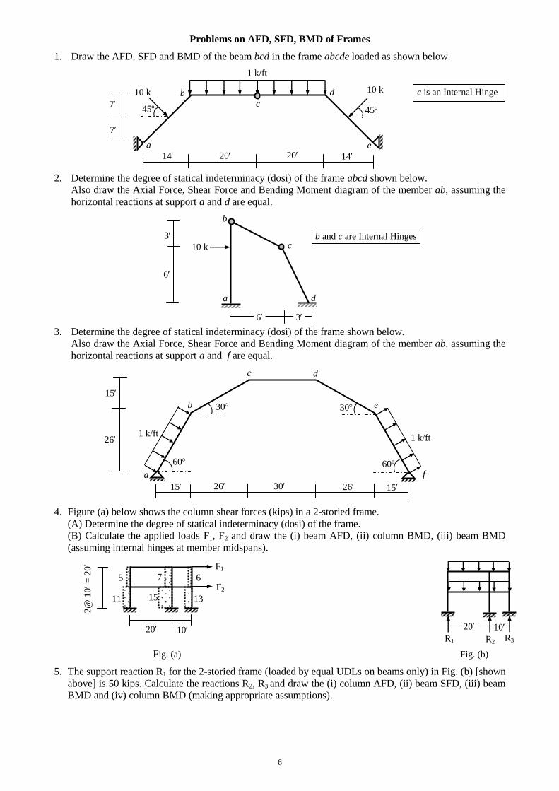
Problems on AFD, SFD, BMD of Frames
1. Draw the AFD, SFD and BMD of the beam bcd in the frame abcde loaded as shown below.
2. Determine the degree of statical indeterminacy (dosi) of the frame abcd shown below.
Also draw the Axial Force, Shear Force and Bending Moment diagram of the member ab, assuming the
horizontal reactions at support a and d are equal.
3. Determine the degree of statical indeterminacy (dosi) of the frame shown below.
Also draw the Axial Force, Shear Force and Bending Moment diagram of the member ab, assuming the
horizontal reactions at support a and f are equal.
4. Figure (a) below shows the column shear forces (kips) in a 2-storied frame.
(A) Determine the degree of statical indeterminacy (dosi) of the frame.
(B) Calculate the applied loads F1, F2 and draw the (i) beam AFD, (ii) column BMD, (iii) beam BMD
(assuming internal hinges at member midspans).
Fig. (a) Fig. (b)
5. The support reaction R1 for the 2-storied frame (loaded by equal UDLs on beams only) in Fig. (b) [shown
above] is 50 kips. Calculate the reactions R2, R3 and draw the (i) column AFD, (ii) beam SFD, (iii) beam
BMD and (iv) column BMD (making appropriate assumptions).
15
7
11
5
20 10
2@
10
= 2
0
13
6 F2
F1
R1 R2 R3
10 k
3
6
d a
b
c
3 6
b and c are Internal Hinges
20 20 a
c b
7
10 k
14 14
e
d 10 k
7
1 k/ft
c is an Internal Hinge
45º 45º
26 30
a f
c
b
26 1 k/ft
15
15 26 15
e
1 k/ft
60 60
30 30
d
20 10
7
Live Loads and Influence Lines
Live Loads
Live Loads, either moving or movable, produce varying effects in a structure, depending on the location of
the part being considered, the force function being considered (i.e., reaction, shear, bending moment, etc),
and the position of the loads producing the effect. It is necessary to determine the critical position of the
loading system which will produce the greatest force (i.e., reaction, shear or bending moment) and to
calculate that force after having found the critical position.
Influence Lines
An influence line is a diagram showing the variation of a particular force (i.e., reaction, shear, bending
moment at a section, stress at a point or other direct function) due to a unit load moving across the structure.
Influence Line can be defined to be a curve the ordinate of which at any point equals the value of some
particular function due to a unit load (say 1-lb load) acting at that point, and is constructed by plotting
directly under the point where the unit load is placed an ordinate the height of which represents the value of
the particular function being studied when the load is in that position. Influence Lines are often useful in
studying the effect of a system of moving loads across a structure.
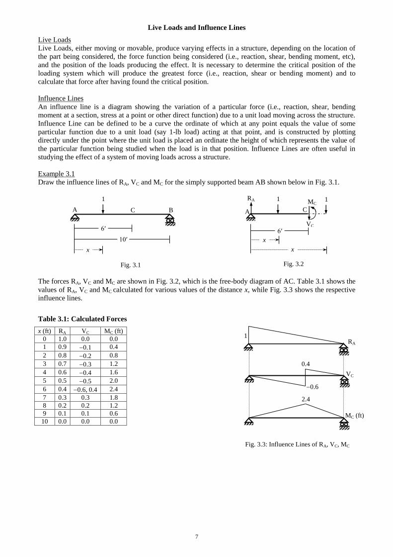
Example 3.1
Draw the influence lines of RA, VC and MC for the simply supported beam AB shown below in Fig. 3.1.
The forces RA, VC and MC are shown in Fig. 3.2, which is the free-body diagram of AC. Table 3.1 shows the
values of RA, VC and MC calculated for various values of the distance x, while Fig. 3.3 shows the respective
influence lines.
Table 3.1: Calculated Forces
x (ft) RA VC MC (ft)
0 1.0 0.0 0.0
1 0.9 0.1 0.4
2 0.8 0.2 0.8
3 0.7 0.3 1.2
4 0.6 0.4 1.6
5 0.5 0.5 2.0
6 0.4 0.6, 0.4 2.4
7 0.3 0.3 1.8
8 0.2 0.2 1.2
9 0.1 0.1 0.6
10 0.0 0.0 0.0
C A B
6′
10′
x
1 1
x
C A
MC
VC 6′
RA
Fig. 3.1 Fig. 3.2
x
1
RA
VC
MC (ft)
1
0.6
0.4
2.4
Fig. 3.3: Influence Lines of RA, VC, MC
8
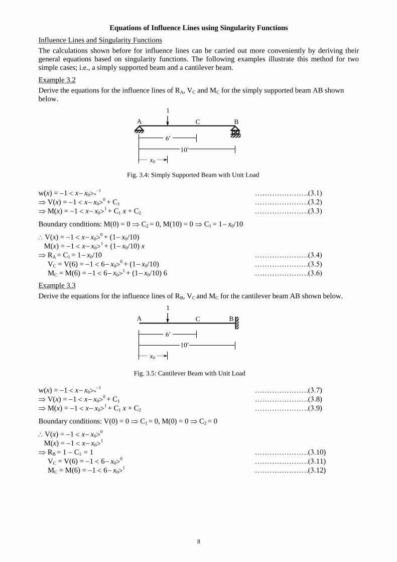
Equations of Influence Lines using Singularity Functions
Influence Lines and Singularity Functions
The calculations shown before for influence lines can be carried out more conveniently by deriving their
general equations based on singularity functions. The following examples illustrate this method for two
simple cases; i.e., a simply supported beam and a cantilever beam.
Example 3.2
Derive the equations for the influence lines of RA, VC and MC for the simply supported beam AB shown
below.
w(x) = 1 x x0*1
………………….(3.1)
V(x) = 1 x x00 + C1 ………………….(3.2)
M(x) = 1 x x01 + C1 x + C2 ………………….(3.3)
Boundary conditions: M(0) = 0 C2 = 0, M(10) = 0 C1 = 1 x0/10
V(x) = 1 x x00 + (1 x0/10)
M(x) = 1 x x01 + (1 x0/10) x
RA = C1 = 1 x0/10 ………………….(3.4)
VC = V(6) = 1 6 x00 + (1 x0/10) ………………….(3.5)
MC = M(6) = 1 6 x01 + (1 x0/10) 6 ………………….(3.6)
Example 3.3
Derive the equations for the influence lines of RB, VC and MC for the cantilever beam AB shown below.
w(x) = 1 x x0*1
………………….(3.7)
V(x) = 1 x x00 + C1 ………………….(3.8)
M(x) = 1 x x01 + C1 x + C2 ………………….(3.9)
Boundary conditions: V(0) = 0 C1 = 0, M(0) = 0 C2 = 0
V(x) = 1 x x00
M(x) = 1 x x01
RB = 1 C1 = 1 ………………….(3.10)
VC = V(6) = 1 6 x00 ………………….(3.11)
MC = M(6) = 1 6 x01 ………………….(3.12)
C A B
1
6′
x0
10′
C A B
1
6′
x0
10′
Fig. 3.4: Simply Supported Beam with Unit Load
Fig. 3.5: Cantilever Beam with Unit Load
9
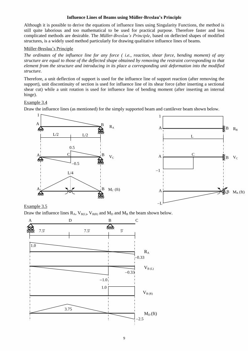
Influence Lines of Beams using Müller-Breslau’s Principle
Although it is possible to derive the equations of influence lines using Singularity Functions, the method is
still quite laborious and too mathematical to be used for practical purpose. Therefore faster and less
complicated methods are desirable. The Müller-Breslau’s Principle, based on deflected shapes of modified
structures, is a widely used method particularly for drawing qualitative influence lines of beams.
Müller-Breslau’s Principle
The ordinates of the influence line for any force ( i.e., reaction, shear force, bending moment) of any
structure are equal to those of the deflected shape obtained by removing the restraint corresponding to that
element from the structure and introducing in its place a corresponding unit deformation into the modified
structure.
Therefore, a unit deflection of support is used for the influence line of support reaction (after removing the
support), unit discontinuity of section is used for influence line of its shear force (after inserting a sectional
shear cut) while a unit rotation is used for influence line of bending moment (after inserting an internal
hinge).
Example 3.4
Draw the influence lines (as mentioned) for the simply supported beam and cantilever beam shown below.
Example 3.5
Draw the influence lines RA, VB(L), VB(R) and MD and MB the beam shown below.
A D B C
7.5 7.5 5
RA
VB (L)
1.0 VB (R)
MD (ft) 2.5
RA
VC
MC (ft)
A
A
A
B
B
B
A
A
A
B
B
B
RB
VC
MB (ft)
C C
1
1
L
1
0.5
0.5
L/4
L/2 L/2 L
3.75
1.0
1.0
0.33
0.33
10
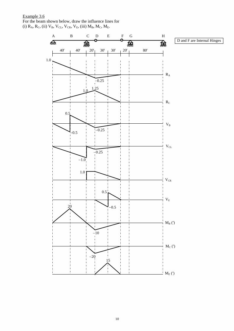
Example 3.6
For the beam shown below, draw the influence lines for
(i) RA, RC, (ii) VB, VCL, VCR, VE, (iii) MB, MC, ME.
A B C D E F G H
40 40 20 30 30 20 80
D and F are Internal Hinges
RA
RC
VB
VCL
VCR
VE
MB (′)
MC (′)
ME (′)
1.0
1.0
0.5
0.5
1.0
1.0
0.5
0.5 20
10
20 15
0.25
0.25
1.25
0.25
11
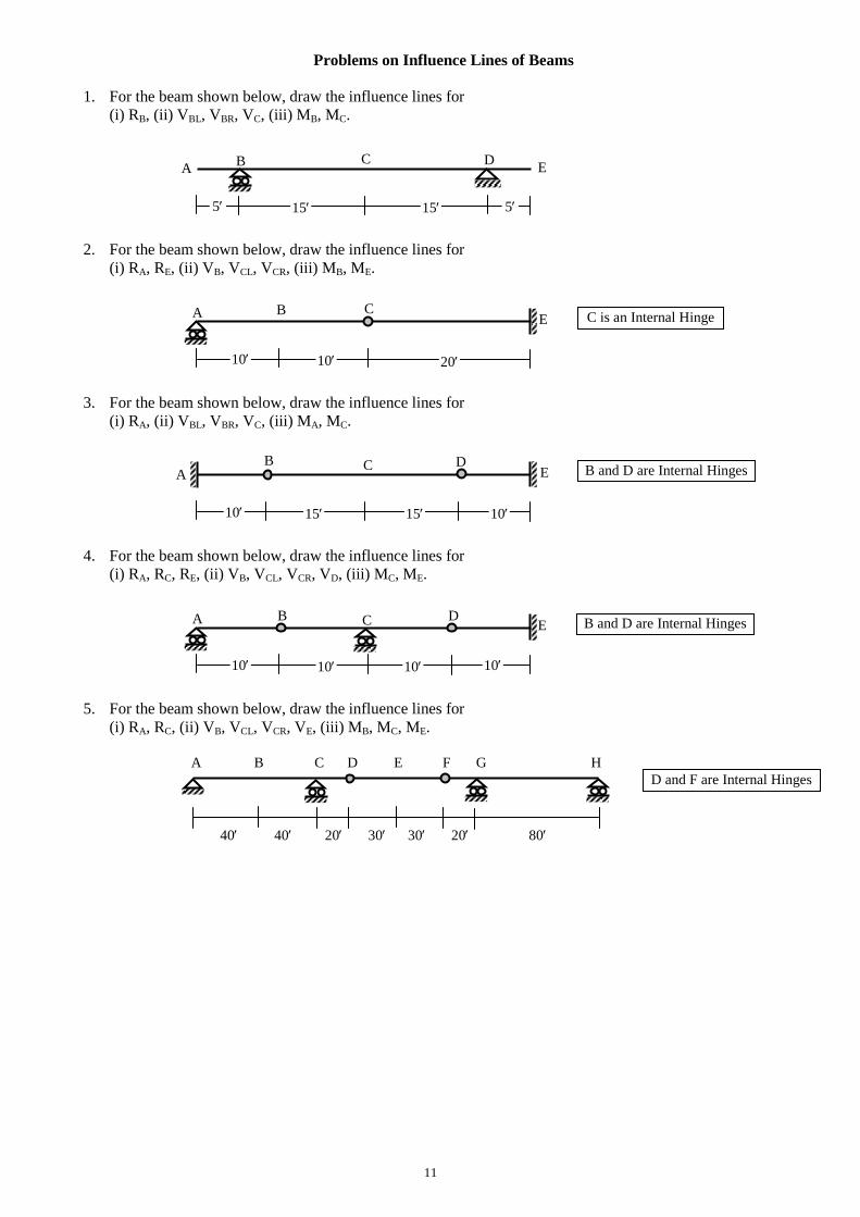
Problems on Influence Lines of Beams
1. For the beam shown below, draw the influence lines for
(i) RB, (ii) VBL, VBR, VC, (iii) MB, MC.
2. For the beam shown below, draw the influence lines for
(i) RA, RE, (ii) VB, VCL, VCR, (iii) MB, ME.
3. For the beam shown below, draw the influence lines for
(i) RA, (ii) VBL, VBR, VC, (iii) MA, MC.
4. For the beam shown below, draw the influence lines for
(i) RA, RC, RE, (ii) VB, VCL, VCR, VD, (iii) MC, ME.
5. For the beam shown below, draw the influence lines for
(i) RA, RC, (ii) VB, VCL, VCR, VE, (iii) MB, MC, ME.
A B C D E F G H
40 40 20 30 30 20 80
D and F are Internal Hinges
B and D are Internal Hinges
10 10 10 10
B A C D E
C is an Internal Hinge
20 10 10
B A C E
15 5 5
B A
C E
15
D
B and D are Internal Hinges
15 10 10
B A
C E
15
D
12
Influence Lines of Frames
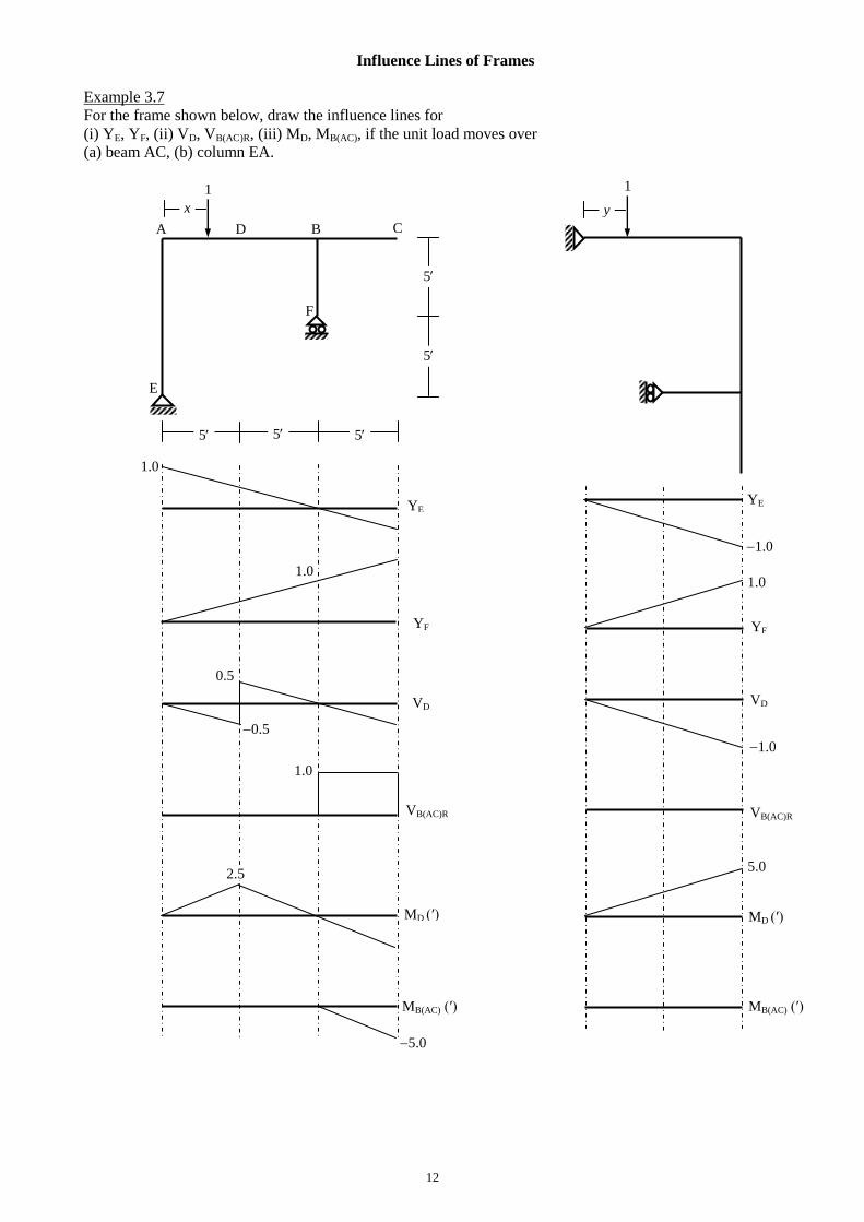
Example 3.7
For the frame shown below, draw the influence lines for
(i) YE, YF, (ii) VD, VB(AC)R, (iii) MD, MB(AC), if the unit load moves over
(a) beam AC, (b) column EA.
5 5
5
5
D A B
F
C
5
E
1.0
1.0
1.0
0.5
0.5
2.5
5.0
MB(AC) (′)
YE
YF
VD
VB(AC)R
MD (′)
x
1
y
1
YE
YF
VD
VB(AC)R
MD (′)
MB(AC) (′)
1.0
1.0
5.0
1.0
13
Influence Lines of Frames using Müller-Breslau’s Principle
7.5
5
E A B
C
7.5
D
5
5
D A B
E
5
F
C
5
5
XE 1.0
1.0
1.0 1.0
0.5
YE
VG
VD
MB(AC) (′)
MD (′)
G
1.0 1.0
0.5
1.0 1.0
5.0 5.0
7.5
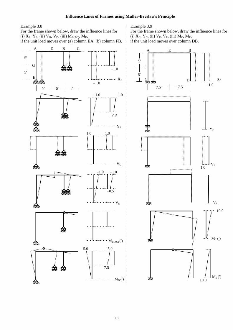
Example 3.8
For the frame shown below, draw the influence lines for
(i) XE, YE, (ii) VG, VD, (iii) MB(AC), MD,
if the unit load moves over (a) column EA, (b) column FB.
Example 3.9
For the frame shown below, draw the influence lines for
(i) XC, YC, (ii) VF, VE, (iii) MC, ME,
if the unit load moves over column DB.
XC
YC
F
5
VF
VE
MC (′)
ME (′)
1.0
1.0
10.0
10.0
14
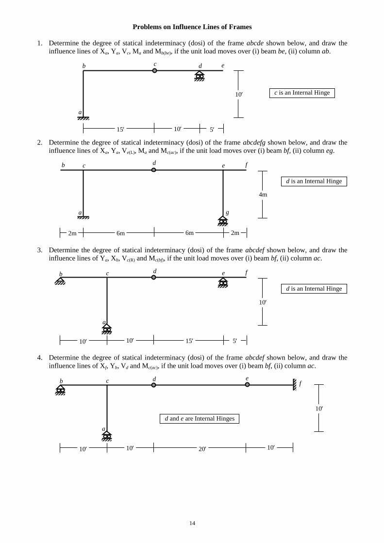
Problems on Influence Lines of Frames
1. Determine the degree of statical indeterminacy (dosi) of the frame abcde shown below, and draw the
influence lines of Xa, Ya, Vc, Ma and Mb(be), if the unit load moves over (i) beam be, (ii) column ab.
2. Determine the degree of statical indeterminacy (dosi) of the frame abcdefg shown below, and draw the
influence lines of Xa, Ya, Ve(L), Ma and Mc(ac), if the unit load moves over (i) beam bf, (ii) column eg.
3. Determine the degree of statical indeterminacy (dosi) of the frame abcdef shown below, and draw the
influence lines of Ya, Xb, Vc(R) and Mc(bf), if the unit load moves over (i) beam bf, (ii) column ac.
4. Determine the degree of statical indeterminacy (dosi) of the frame abcdef shown below, and draw the
influence lines of Xf, Yb, Vd and Mc(ac), if the unit load moves over (i) beam bf, (ii) column ac.
10
c b d e
a
15 10 5
4m
c b d e
a
6m 6m 2m
f
g
2m
d is an Internal Hinge
10
c b d e
a
15
5
f
10
d is an Internal Hinge
10
10
c b d e
a
20
10
f
10
d and e are Internal Hinges
10
c is an Internal Hinge
15
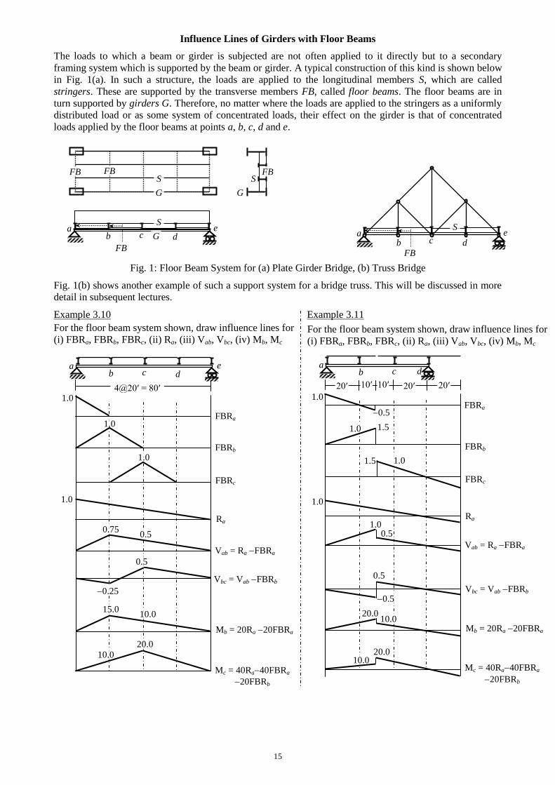
Influence Lines of Girders with Floor Beams
The loads to which a beam or girder is subjected are not often applied to it directly but to a secondary
framing system which is supported by the beam or girder. A typical construction of this kind is shown below
in Fig. 1(a). In such a structure, the loads are applied to the longitudinal members S, which are called
stringers. These are supported by the transverse members FB, called floor beams. The floor beams are in
turn supported by girders G. Therefore, no matter where the loads are applied to the stringers as a uniformly
distributed load or as some system of concentrated loads, their effect on the girder is that of concentrated
loads applied by the floor beams at points a, b, c, d and e.
Fig. 1: Floor Beam System for (a) Plate Girder Bridge, (b) Truss Bridge
Fig. 1(b) shows another example of such a support system for a bridge truss. This will be discussed in more
detail in subsequent lectures.
Example 3.10 Example 3.11
FB
G
S FB
S
FB
G
G
S FB
a b c d
e a
b c d e
FB
S
a b c d
e
For the floor beam system shown, draw influence lines for
(i) FBRa, FBRb, FBRc, (ii) Ra, (iii) Vab, Vbc, (iv) Mb, Mc
1.0
1.0
1.0
1.0
0.75
0.5
0.25
4@20′ = 80′
15.0
FBRa
FBRb
FBRc
Ra
Vab = Ra FBRa
Vbc = Vab FBRb
Mb = 20Ra 20FBRa
Mc = 40Ra40FBRa
20FBRb
20.0 10.0
10.0
0.5
For the floor beam system shown, draw influence lines for
(i) FBRa, FBRb, FBRc, (ii) Ra, (iii) Vab, Vbc, (iv) Mb, Mc
a b c d
20′
FBRa
FBRb
FBRc
Ra
Vab = Ra FBRa
Vbc = Vab FBRb
Mb = 20Ra 20FBRa
Mc = 40Ra40FBRa
20FBRb
20′ 20′ 10′ 10′
1.0
1.0
1.0
1.0
1.5
1.5
0.5
0.5 1.0
10.0 20.0
0.5
0.5
20.0 10.0
16
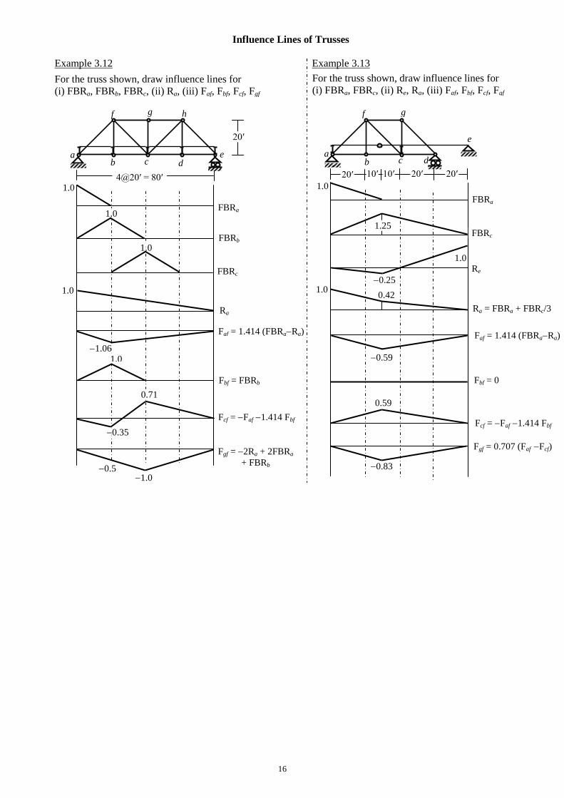
Influence Lines of Trusses
Example 3.12 Example 3.13
a b c d
e
For the truss shown, draw influence lines for
(i) FBRa, FBRb, FBRc, (ii) Ra, (iii) Faf, Fbf, Fcf, Fgf
1.0
1.0
1.0
1.0
1.06
4@20′ = 80′
0.35
FBRa
FBRb
FBRc
Ra
Faf = 1.414 (FBRaRa)
Fbf = FBRb
Fcf = Faf 1.414 Fbf
Fgf = 2Ra + 2FBRa
+ FBRb
1.0 0.5
0.71
For the truss shown, draw influence lines for
(i) FBRa, FBRc, (ii) Re, Ra, (iii) Faf, Fbf, Fcf, Fgf
a b c d
20′
FBRa
FBRc
Re
Ra = FBRa + FBRc/3
20′ 20′ 10′ 10′
1.0
1.0
1.0
1.25
0.25
f g h f g
1.0
20′ e
Fbf = 0
Fgf = 0.707 (Faf Fcf)
0.42
0.59
0.59
0.83
Faf = 1.414 (FBRaRa)
Fcf = Faf 1.414 Fbf
17
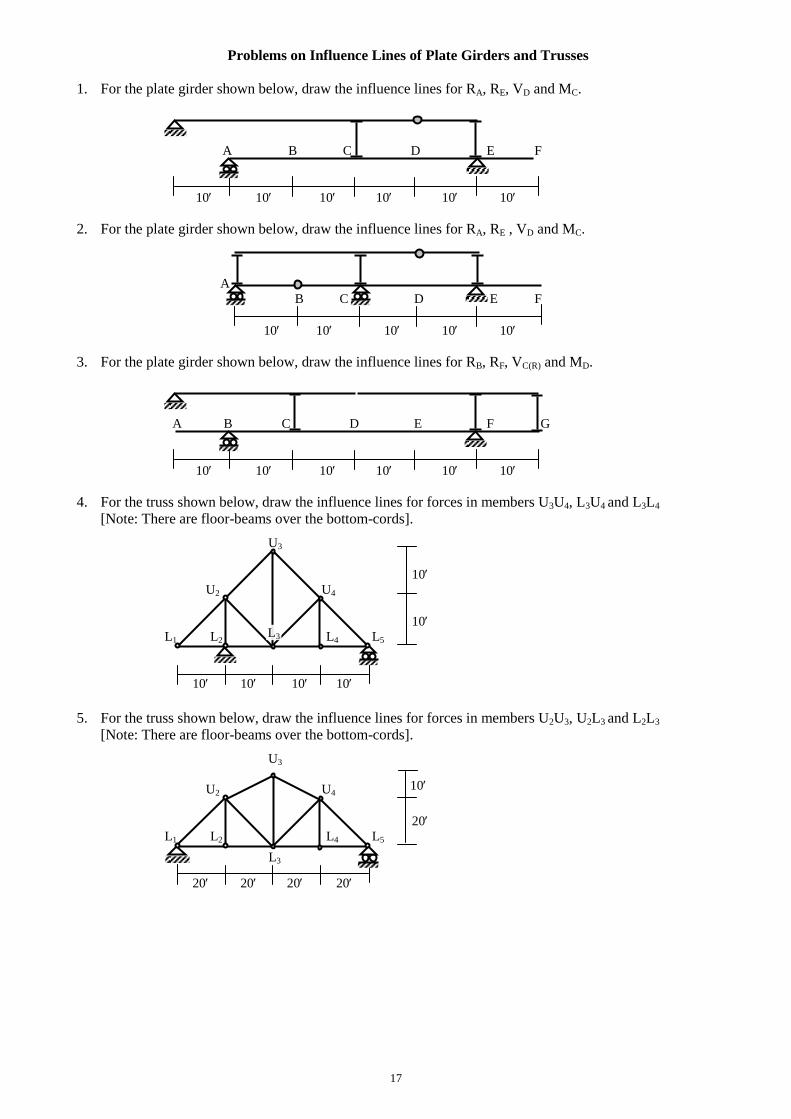
Problems on Influence Lines of Plate Girders and Trusses
1. For the plate girder shown below, draw the influence lines for RA, RE, VD and MC.
A B C D E F
10 10 10 10 10 10
2. For the plate girder shown below, draw the influence lines for RA, RE , VD and MC.
A
B C D E F
10 10 10 10 10
3. For the plate girder shown below, draw the influence lines for RB, RF, VC(R) and MD.
A B C D E F G
10 10 10 10 10 10
4. For the truss shown below, draw the influence lines for forces in members U3U4, L3U4 and L3L4
[Note: There are floor-beams over the bottom-cords].
U3
10
U2 U4
10
L1 L2 L4 L5
10 10 10 10 5. For the truss shown below, draw the influence lines for forces in members U2U3, U2L3 and L2L3
[Note: There are floor-beams over the bottom-cords].
U3
U2 U4
20
L1 L2 L4 L5
20 20 20 20
10
L3
L3

18
Force Calculation using Influence Lines
Application of Influence Lines
Force Calculation for Concentrated Loads
………………..Eq. (3.1)
Force Calculation for Uniformly Distributed Loads
………………..Eq. (3.2)
Example 3.14
19
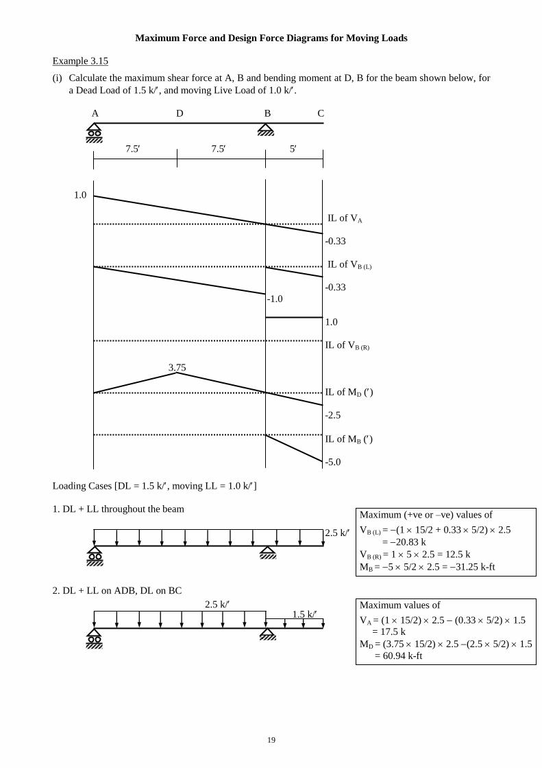
Maximum Force and Design Force Diagrams for Moving Loads
Example 3.15
(i) Calculate the maximum shear force at A, B and bending moment at D, B for the beam shown below, for
a Dead Load of 1.5 k/, and moving Live Load of 1.0 k/.
A D B C
7.5 7.5 5
1.0
IL of VA
-0.33
IL of VB (L)
-0.33
-1.0
1.0
IL of VB (R)
IL of MD ()
-2.5
IL of MB ()
-5.0
Loading Cases [DL = 1.5 k/, moving LL = 1.0 k/]
1. DL + LL throughout the beam
2.5 k/
2. DL + LL on ADB, DL on BC
1.5 k/
2.5 k/
3.75
Maximum (+ve or –ve) values of
VB (L) = (1 15/2 + 0.33 5/2) 2.5
= 20.83 k
VB (R) = 1 5 2.5 = 12.5 k
MB = 5 5/2 2.5 = 31.25 k-ft
Maximum values of
VA = (1 15/2) 2.5 (0.33 5/2) 1.5
= 17.5 k
MD = (3.75 15/2) 2.5 (2.5 5/2) 1.5
= 60.94 k-ft

20
(ii) Draw the design Shear Force and Bending Moment Diagrams of the beam loaded as described before.
Case 1
16.67
12.5
SFD (k)
55.56 -20.83
BMD (k)
-31.25
Case 2
17.5
7.5
SFD (k)
61.25
-20.0
BMD (k)
-18.75
Design SFD and BMD
17.5 12.5
Design SFD (k)
61.25 -20.83
Design BMD (k)
-31.25
21
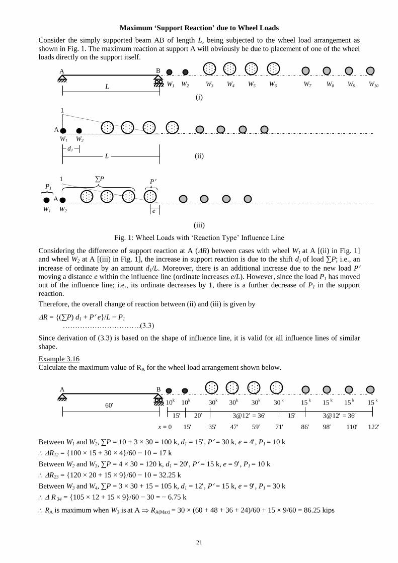
Maximum ‘Support Reaction’ due to Wheel Loads
Consider the simply supported beam AB of length L, being subjected to the wheel load arrangement as
shown in Fig. 1. The maximum reaction at support A will obviously be due to placement of one of the wheel
loads directly on the support itself.
L
(i)
(ii)
(iii)
Fig. 1: Wheel Loads with ‘Reaction Type’ Influence Line
Considering the difference of support reaction at A (R) between cases with wheel W1 at A [(ii) in Fig. 1]
and wheel W2 at A [(iii) in Fig. 1], the increase in support reaction is due to the shift d1 of load ∑P; i.e., an
increase of ordinate by an amount d1/L. Moreover, there is an additional increase due to the new load P moving a distance e within the influence line (ordinate increases e/L). However, since the load P1 has moved
out of the influence line; i.e., its ordinate decreases by 1, there is a further decrease of P1 in the support
reaction.
Therefore, the overall change of reaction between (ii) and (iii) is given by
R = {(∑P) d1 + P e}/L − P1
…………………………..(3.3)
Since derivation of (3.3) is based on the shape of influence line, it is valid for all influence lines of similar
shape.
Example 3.16
Calculate the maximum value of RA for the wheel load arrangement shown below.
60
15 20 3@12 = 36 15 3@12 = 36
Between W1 and W2, ∑P = 10 + 3 × 30 = 100 k, d1 = 15, P = 30 k, e = 4, P1 = 10 k
R12 = {100 × 15 + 30 × 4}/60 − 10 = 17 k
Between W2 and W3, ∑P = 4 × 30 = 120 k, d1 = 20, P = 15 k, e = 9, P1 = 10 k
R23 = {120 × 20 + 15 × 9}/60 − 10 = 32.25 k
Between W3 and W4, ∑P = 3 × 30 + 15 = 105 k, d1 = 12, P = 15 k, e = 9, P1 = 30 k
R 34 = {105 × 12 + 15 × 9}/60 − 30 = − 6.75 k
RA is maximum when W3 is at A RA(Max) = 30 × (60 + 48 + 36 + 24)/60 + 15 × 9/60 = 86.25 kips
A
A
1
1
W1 W2
W1 W2
∑P P P1
d1 L
e
A B
W1 W2 W3 W4 W5 W6 W7 W8 W9 W10
A B
10k 10
k 30
k 30
k 30
k 30
k 15
k 15
k 15
k 15
k
x = 0 15 35 47 59 71 86 98 110 122
22
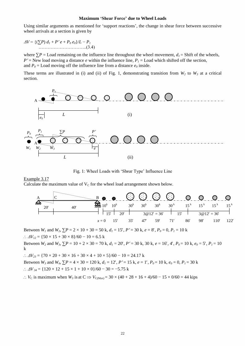
Maximum ‘Shear Force’ due to Wheel Loads
Using similar arguments as mentioned for ‘support reactions’, the change in shear force between successive
wheel arrivals at a section is given by
V = {(∑P) d1 + P e + P0 e0}/L − P1
…………………………..(3.4)
where ∑P = Load remaining on the influence line throughout the wheel movement, d1 = Shift of the wheels,
P = New load moving a distance e within the influence line, P1 = Load which shifted off the section,
and P0 = Load moving off the influence line from a distance e0 inside.
These terms are illustrated in (i) and (ii) of Fig. 1, demonstrating transition from W2 to W3 at a critical
section.
L (i)
L (ii)
Fig. 1: Wheel Loads with ‘Shear Type’ Influence Line
Example 3.17
Calculate the maximum value of VC for the wheel load arrangement shown below.
20 40
15 20 3@12 = 36 15 3@12 = 36
Between W1 and W2, ∑P = 2 × 10 + 30 = 50 k, d1 = 15, P = 30 k, e = 8, P0 = 0, P1 = 10 k
V12 = {50 × 15 + 30 × 8}/60 − 10 = 6.5 k
Between W2 and W3, ∑P = 10 + 2 × 30 = 70 k, d1 = 20, P = 30 k, 30 k, e = 16, 4, P0 = 10 k, e0 = 5, P1 = 10
k
V23 = {70 × 20 + 30 × 16 + 30 × 4 + 10 × 5}/60 − 10 = 24.17 k
Between W3 and W4, ∑P = 4 × 30 = 120 k, d1 = 12, P = 15 k, e = 1, P0 = 10 k, e0 = 0, P1 = 30 k
V 34 = {120 × 12 + 15 × 1 + 10 × 0}/60 − 30 = −5.75 k
VC is maximum when W3 is at C VC(Max) = 30 × (40 + 28 + 16 + 4)/60 − 15 × 0/60 = 44 kips
A B
10k 10
k 30
k 30
k 30
k 30
k 15
k 15
k 15
k 15
k
x = 0 15 35 47 59 71 86 98 110 122
A
e0
A W1 W2 W3
∑P P P0
e
P1
P1
C
23
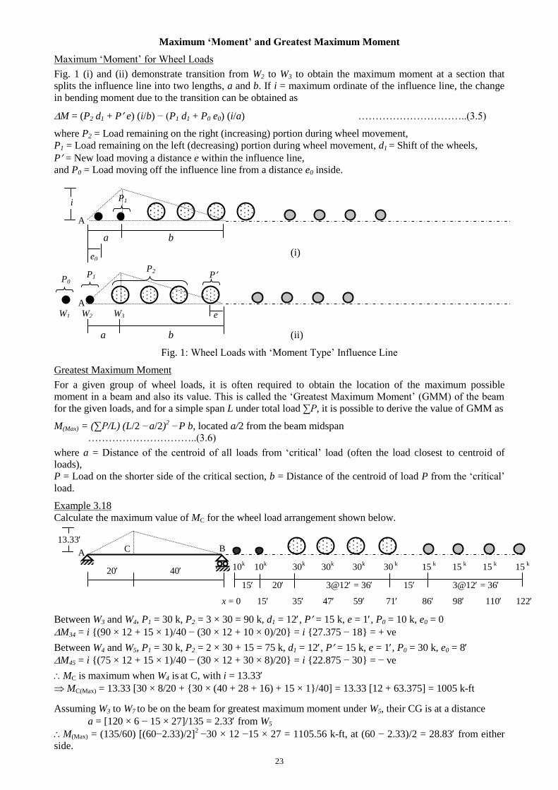
Maximum ‘Moment’ and Greatest Maximum Moment
Maximum ‘Moment’ for Wheel Loads
Fig. 1 (i) and (ii) demonstrate transition from W2 to W3 to obtain the maximum moment at a section that
splits the influence line into two lengths, a and b. If i = maximum ordinate of the influence line, the change
in bending moment due to the transition can be obtained as
M = (P2 d1 + P e) (i/b) − (P1 d1 + P0 e0) (i/a) …………………………..(3.5)
where P2 = Load remaining on the right (increasing) portion during wheel movement,
P1 = Load remaining on the left (decreasing) portion during wheel movement, d1 = Shift of the wheels,
P = New load moving a distance e within the influence line,
and P0 = Load moving off the influence line from a distance e0 inside.
a b
(i)
a b (ii)
Fig. 1: Wheel Loads with ‘Moment Type’ Influence Line
Greatest Maximum Moment
For a given group of wheel loads, it is often required to obtain the location of the maximum possible
moment in a beam and also its value. This is called the ‘Greatest Maximum Moment’ (GMM) of the beam
for the given loads, and for a simple span L under total load ∑P, it is possible to derive the value of GMM as
M(Max) = (∑P/L) (L/2 −a/2)2 −P b, located a/2 from the beam midspan
…………………………..(3.6)
where a = Distance of the centroid of all loads from ‘critical’ load (often the load closest to centroid of
loads),
P = Load on the shorter side of the critical section, b = Distance of the centroid of load P from the ‘critical’
load.
Example 3.18
Calculate the maximum value of MC for the wheel load arrangement shown below.
20 40
15 20 3@12 = 36 15 3@12 = 36
Between W3 and W4, P1 = 30 k, P2 = 3 × 30 = 90 k, d1 = 12, P = 15 k, e = 1, P0 = 10 k, e0 = 0
M34 = i {(90 × 12 + 15 × 1)/40 − (30 × 12 + 10 × 0)/20} = i {27.375 − 18} = + ve
Between W4 and W5, P1 = 30 k, P2 = 2 × 30 + 15 = 75 k, d1 = 12, P = 15 k, e = 1, P0 = 30 k, e0 = 8
M45 = i {(75 × 12 + 15 × 1)/40 − (30 × 12 + 30 × 8)/20} = i {22.875 − 30} = − ve
MC is maximum when W4 is at C, with i = 13.33
MC(Max) = 13.33 [30 × 8/20 + {30 × (40 + 28 + 16) + 15 × 1}/40] = 13.33 [12 + 63.375] = 1005 k-ft
Assuming W3 to W7 to be on the beam for greatest maximum moment under W5, their CG is at a distance
a = [120 × 6 − 15 × 27]/135 = 2.33 from W5
M(Max) = (135/60) [(60−2.33)/2]2
−30 × 12 −15 × 27 = 1105.56 k-ft, at (60 − 2.33)/2 = 28.83 from either
side.
A B
10k 10
k 30
k 30
k 30
k 30
k 15
k 15
k 15
k 15
k
x = 0 15 35 47 59 71 86 98 110 122
A
e0
A W1 W2 W3
P2 P
P0
e
P1
P1
C
i
13.33
24
Problems on Load Calculation using Influence Lines
1. For the truss shown below, calculate the maximum tension and compression in members U4L5, U3U4,
L3U4 and L3L4 for a uniformly distributed dead load of 1 k/ft and a concentrated live load of 20 k
[Note: Stringers are simply supported on floor-beams at bottom-cord joints].
U3
10
U2 U4
10
L1 L2 L4 L5
10 10 10 10
2. For the beam shown below, calculate the maximum and minimum values of
(i) RA, RC, (ii) VB, VCL, VCR, VE, (iii) MB, MC, ME
for a uniformly distributed dead load of 1 k/ft and a live load of 2 k/ft.
A B C D E F G H
50 50 30 40 40 30 100
3. For the beam loaded as described in Question 2, use the influence lines of
(i) VA, VC(L) to draw the Design SFD, and (ii) MB, MC to draw the Design BMD.
4. Calculate the maximum values of RC, VE, MC and ME for the beam described in Question 2, using both
the wheel loads shown below.
10
k 10
k 40
k 40
k 20
k 4
k 16
k 16
k
10 10 10 10 14 14
Wheel Loads 1 Wheel Loads 2
5. Use both the wheel loads described in Question 4 to calculate the greatest maximum moment within the
span DF of the beam described in Question 2.
6. For the Wheel Loads1 shown in Question 4, calculate the maximum values of FBRA, RC, VD(R) and MD
for the plate girder shown below.
A F
B C D E
10 10 10 10 10
7. For the truss shown below, calculate the maximum reaction at support L5 and maximum forces in
members U2U3 and L2L3 for the (i) distributed loads described in Question 1, (ii) Wheel Loads1 shown
in Question 4 [Note: Stringers are simply supported on floor-beams at bottom-cord joints].
U2 U4
20
L1 L2 L4 L5
20 20 20 20
L3
D and F are Internal Hinges
10
L3
U3
25
Wind Pressure and Coefficients
Basic Wind Pressure
The basic wind pressure on a surface is given by qb = air Vb2/2 .……….(1)
where air = Density of air = 0.0765/32.2 = 23.76 10-4
slug/ft3
Vb = Basic wind speed, ft/sec = 1.467 Basic wind speed, mph
Eq. (1) qb = 23.76 10-4
(1.467 Vb)2/2 = 0.00256 Vb
2 .……….(2)
where qb is in psf (lb/ft2) and Vb is in mph (mile/hr).
The basic wind speeds at different important locations of Bangladesh are given below. A more detailed map
for the entire country is available in BNBC 1993.
Sustained Wind Pressure
The wind velocity (and pressure) increases from zero at the base of the structure and is also a function of the
exposure (i.e., open terrain or congested area). Moreover one has to account for the importance of the
structure; i.e., design the sensitive structures more conservatively.
The sustained wind pressure on a building surface at any height z above ground is given by
qz = 0.00256 CI Cz Vb2 .……….(3)
where CI = Structural importance coefficient, Cz = Height and exposure coefficient.
Design Wind Pressure
The design wind pressure can be calculated by multiplying the sustained wind pressure by appropriate
pressure coefficients due to wind gust and turbulence as well as local topography.
The design wind pressure on a surface at any height z above ground is given by
pz = CG Ct Cp qz .……….(4)
where CG = Wind gust coefficient, Ct = Local topography coefficient, Cp = Pressure coefficient.
Height z (ft) Cz
Exp A Exp B Exp C
0~15 0.368 0.801 1.196
50 0.624 1.125 1.517
100 0.849 1.371 1.743
150 1.017 1.539 1.890
200 1.155 1.671 2.002
300 1.383 1.876 2.171
400 1.572 2.037 2.299
500 1.736 2.171 2.404
650 1.973 2.357 2.547
1000 2.362 2.595 2.724
Location Vb (mph)
Dhaka 130
Chittagong 160
Rajshahi 95
Khulna 150
Category CI
Essential facilities 1.25
Hazardous facilities 1.25
Special occupancy 1.00
Standard occupancy 1.00
Low-risk structure 0.80

26
The value of CG for slender structures (height 5 times the minimum width) would be determined by
dynamic analysis. Although code-based formulae are available, it is unlikely to exceed 2.0.
The pressure coefficient Cp for rectangular buildings with flat roofs may be obtained as follows
The pressure coefficient Cp for the windward surfaces of trusses or inclined surfaces are approximated by
Cp = 0.7, for 0 20
Cp = (0.072.1), for 20 30
Cp = (0.030.9), for 30 60
Cp = 0.9, for 60 90 ……….…(5(a)~(d))
For leeward surface, Cp = 0.7, for any value of …...………….(5(e))
Vortex Induced Vibration (VIV)
This phenomenon, has been (and still is) extensively studied in various branches of structural as well as fluid
dynamics. The pressure difference around a bluff body in flowing fluid may result in separated flow and
shear layers over a large portion of its surface. The outermost shear layers (in contact with the fluid) move
faster than the innermost layers, which are in contact with the structure. If the fluid velocity is large enough,
this causes the shear layers to roll into the near wake and form periodic vortices. The interaction of the
structure with these vortices causes it to vibrate transverse to the flow direction, and this vibration is called
VIV.
The frequency of vortex-shedding is called Strouhal frequency (after Strouhal 1878) and is given by the
simple equation
fs = SU/D .…………….(6)
where U = Fluid Velocity, D = Transverse dimension of the structure, S = Strouhal number, which is a
function of Reynolds number and the geometry of the structure. For circular cylinders, S 0.20.
Height z (ft) CG (for non-slender structures)
Exp A Exp B Exp C
0~15 1.654 1.321 1.154
50 1.418 1.215 1.097
100 1.309 1.162 1.067
150 1.252 1.133 1.051
200 1.215 1.114 1.039
300 1.166 1.087 1.024
400 1.134 1.070 1.013
500 1.111 1.057 1.005
650 1.082 1.040 1.000
1000 1.045 1.018 1.000
H
Wind
Lu H/2
L0 1.5 Lu, 2.5H
* L0/1.5
*
* *
H/2Lu Ct
0.05 1.19
0.10 1.39
0.20 1.85
0.30 2.37
h/B L/B
0.1 0.5 0.65 1.0 2.0 3.0
0.5 1.40 1.45 1.55 1.40 1.15 1.10
1.0 1.55 1.85 2.00 1.70 1.30 1.15
2.0 1.80 2.25 2.55 2.00 1.40 1.20
4.0 1.95 2.50 2.80 2.20 1.60 1.25
Wind h
L L
B

27
Graphs for Wind Coefficients
Fig. 2.2: Gust Response Factor, CG
1.0
1.1
1.2
1.3
1.4
100 130 160 190 220 250
Height (z) above Ground, ft
CG
CG(A) CG(B) CG(C)
Fig. 2.1: Gust Response Factor, CG
1.0
1.2
1.4
1.6
1.8
0 20 40 60 80 100
Height (z) above Ground, ft
CG
CG(A) CG(B) CG(C)
Fig. 1.1: Height and Exposure Coefficient, Cz
0.0
0.5
1.0
1.5
2.0
0 20 40 60 80 100
Height (z) above Ground, ft
Cz
Cz(A) Cz(B) Cz(C)
Fig. 2.3: Gust Response Factors, CG
1.00
1.05
1.10
1.15
1.20
250 400 550 700 850 1000
Height (z) above Ground, ft
CG
CG(A) CG(B) CG(C)
Fig. 3.2: Overall Pressure Coefficient, Cp
1.0
1.2
1.4
1.6
1.8
2.0
2.2
1.0 1.4 1.8 2.2 2.6 3.0
L/B
Cp
h/B = 0.5 h/B = 1.0 h/B = 2.0 h/B = 4.0
Fig. 3.1: Overall Pressure Coefficient, Cp
1.2
1.5
1.8
2.1
2.4
2.7
3.0
0.0 0.2 0.4 0.6 0.8 1.0
L/B
Cp
h/B = 0.5 h/B = 1.0 h/B = 2.0 h/B = 4.0
Fig. 1.2: Height and Exposure Coefficient, Cz
0.5
1.0
1.5
2.0
2.5
100 130 160 190 220 250
Height (z) above Ground, ft
Cz
Cz(A) Cz(B) Cz(C)
Fig. 1.3: Height and Exposure Coefficient, Cz
1.0
1.5
2.0
2.5
3.0
250 400 550 700 850 1000
Height (z) above Ground, ft
Cz
Cz(A) Cz(B) Cz(C)

28
Calculation of Wind Load
Wind Load on a Building
Calculate the wind load at each story of a six-storied hospital building (shown below) located at a flat terrain
in Dhaka. Assume the structure to be subjected to Exposure B.
Side Elevation Building Plan
Solution
The design wind pressure at a height z is given by pz = 0.00256 CI Cz CG Ct Cp Vb2
Since the building is located in Dhaka, the basic wind speed Vb = 130 mph
For the hospital building (essential facility), Structural importance coefficient CI = 1.25
In plane terrain, Local topography coefficient Ct = 1.0
Building height h = 62, dimensions L = 40 and B = 50; i.e., h/B = 1.24 and L/B = 0.80 Cp 1.98
pz = 0.00256 1.25 Cz CG 1.00 1.98 (130)2 = 107.08 Cz CG
The corresponding force Fz = B heff pz = 50 heff pz; where heff = Effective height of the tributary area
heff = 6 + 5 = 11 at 1st floor, (5 + 5 =) 10 between 2
nd and 5
th floor and 5 at 6
th floor
The coefficients Cz, CG and the design wind pressure pz and force Fz at different heights are shown below.
Story z (ft) Cz CG pz (psf) Fz (kips) Fframes (kips)
1 12 0.801 1.321 113.30 62.32 9.35 15.58 12.46 15.58 9.35
2 22 0.866 1.300 120.55 60.27 9.04 15.07 12.05 15.07 9.04
3 32 0.958 1.270 130.28 65.14 9.77 16.29 13.03 16.29 9.77
4 42 1.051 1.239 139.44 69.72 10.46 17.43 13.94 17.43 10.46
5 52 1.135 1.213 147.42 73.71 11.06 18.43 14.74 18.43 11.06
6 62 1.184 1.202 152.39 38.10 5.72 9.53 7.62 9.53 5.72
Wind Load on a Truss
Calculate the wind load at each joint of the industrial truss (30 separated) located at a hilly terrain in
Chittagong (with H = 20, Lu = 100). Assume the structure subjected to Exposure C.
pz (windward) = 0.00256 1.25 1.30 1.10 1.39 (0.24) (160)2 = 39.08 psf
pz (leeward) = 0.00256 1.25 1.30 1.10 1.39 (0.70) (160)2 = 113.98 psf
F (windward, horizontal) = 39.08 30 5/1000 = 5.86 k, 11.72 k and 5.86 k
F (windward, vertical) = 39.08 30 10/1000 = 11.72 k, 23.45 k and 11.72 k
F (leeward, horizontal) = 113.98 30 5/1000 = 17.10 k, 34.20 k and 17.10 k
F (leeward, vertical) = 113.98 30 10/1000 = 34.20 k, 68.40 k and 34.20 k
5@
10=
50
12
15
10
15
10 15 15
10
15
15
10
Wind
20
20
4@20= 80
Solution
Angle = tan-1
(20/40) = 26.6
Cp = (0.07 26.62.1)= 0.24 (windward)
Cp = 0.70 (leeward)
Using Vb = 160 mph, CI = 1.25, H/2Lu = 0.10 Ct = 1.39
and assuming Cz = 1.30, CG = 1.10 (uniform)
29
Seismic Vibration and Structural Response
Earthquakes have been responsible for millions of deaths and an incalculable amount of damage to property.
While they inspired dread and superstitious awe since ancient times, little was understood about them until
the 20th century. Seismology, which involves the scientific study of all aspects of earthquakes, has yielded
plausible answers to such long-standing questions as why and how earthquakes occur.
Cause of Earthquake
According to the Elastic Rebound Theory (Reid 1906), earthquakes are caused by pieces of the crust of the
earth that suddenly shift relative to each other. The most common cause of earthquakes is faulting; i.e., a
break in the earth’s crust along which movement occurs. Most earthquakes occur in narrow belts along the
boundaries of crustal plates, particularly where the plates push together or slide past each other. At times, the
plates are locked together, unable to release the accumulating energy. When this energy grows strong
enough, the plates break free. When two pieces that are next to each other get pushed in different directions,
they will stick together for many years, but eventually the forces pushing on them will cause them to break
apart and move. This sudden shift in the rock shakes the ground around it.
Earthquake Terminology
The point beneath the earth’s surface where the rocks break and move is called the focus of the earthquake.
The focus is the underground point of origin of an earthquake. Directly above the focus, on earth’s surface,
is the epicenter. Earthquake waves reach the epicenter first. During an earthquake, the most violent shaking
is found at the epicenter.
Earthquakes release the strain energy stored within the crustal plates through ‘seismic waves’. There are
three main types of seismic waves. Primary or P-waves vibrate particles along the direction of wave,
Secondary or S-waves that vibrate particles perpendicular to the direction of wave while Raleigh or R-waves
and Love or L-waves move along the surface.
Earthquake Magnitude
A number of measures of earthquake ‘size’ are used for different purposes. From a seismologic point of
view, the most important measure of size is the amount of strain energy released at the source, indicated
quantitatively as the earthquake magnitude. Charles F. Richter introduced the concept of magnitude, which
is the logarithm of the maximum amplitude measured in micrometers (10-6
m) of the earthquake record
obtained by a standard short-period seismograph, corrected to a distance of 100 km; i.e.,
ML = log10 (A/A0) ..………………..(1)
where A is the maximum trace amplitude in micrometers recorded on a seismometer and A0 is a correction
factor as a function of distance. Earthquake intensity is another well-known measure of earthquake severity
at a point, most notable of which is the Modified Marcelli (MM) scale.
Nature of Earthquake Vibration
Earthquake involves vibration of the ground typically for durations of 10~40 seconds, which increases
gradually to the peak amplitude and then decays. It is primarily a horizontal vibration, although some
vertical movement is also present. Since the vibrations are time-dependent, earthquake is essentially a
dynamic problem and the only way to deal with it properly is through dynamic analysis of the structure.
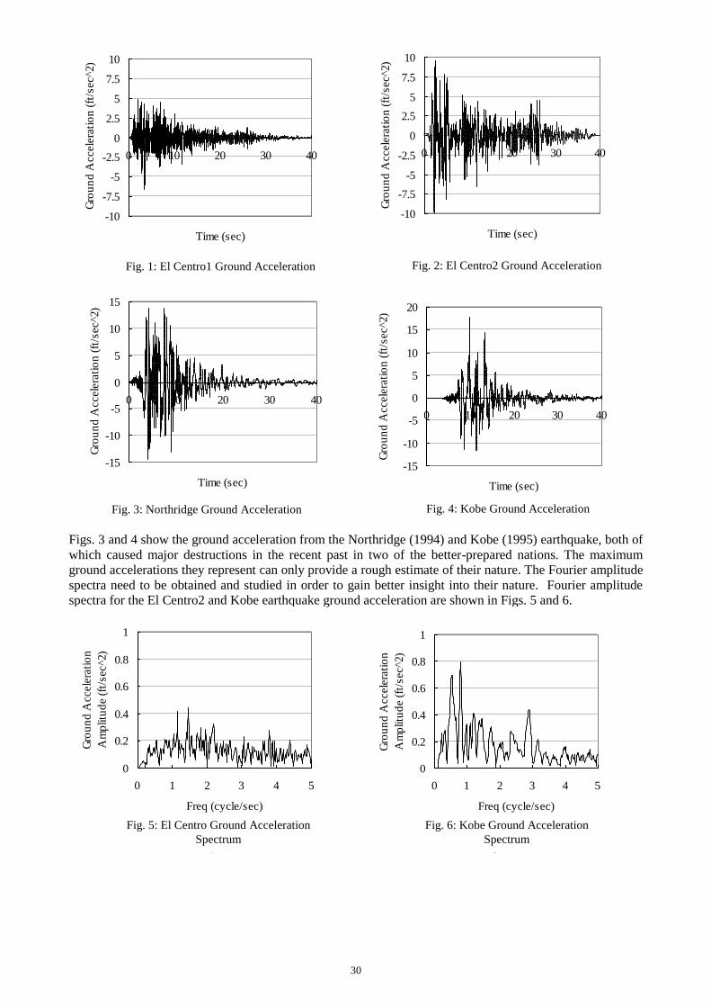
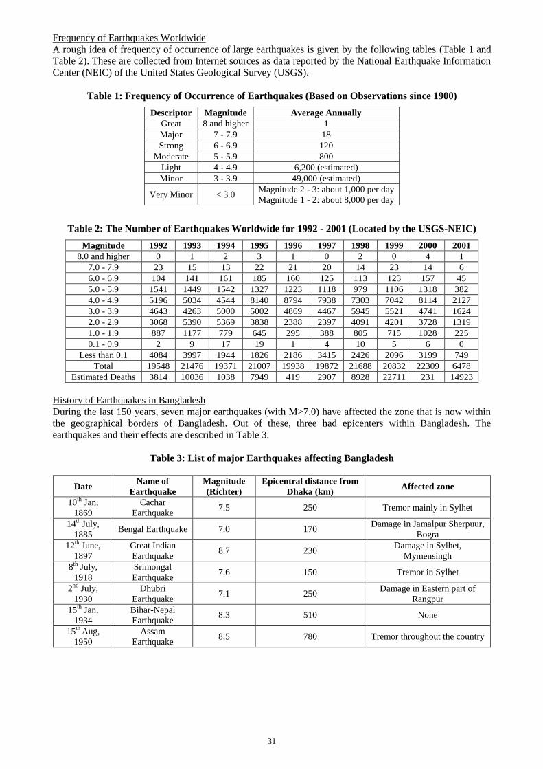
Figs. 1~4 show the temporal variation of ground accelerations recorded during some of the best known and
widely studied earthquakes of the 20th century. The El Centro earthquake (USA, 1940) data has over the last
sixty years been the most used seismic data. However, Figs. 1 and 2 show that the ground accelerations
recorded during this earthquake were different at different stations. It is about 6.61 ft/sec2 for the first station
and 9.92 ft/sec2 for the second, which shows that the location of the recording station should be mentioned
while citing the peak acceleration in an earthquake. The earthquake magnitudes calculated from these data
are also different.
30
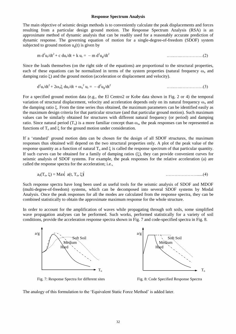
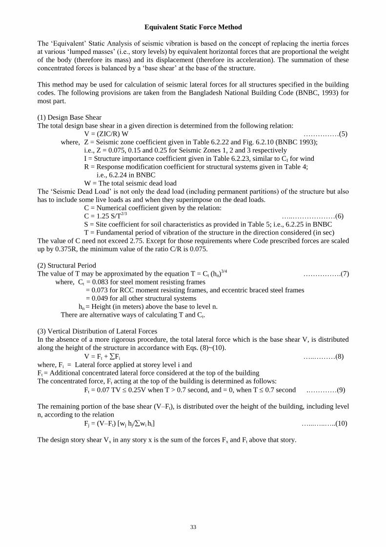
Figs. 3 and 4 show the ground acceleration from the Northridge (1994) and Kobe (1995) earthquake, both of
which caused major destructions in the recent past in two of the better-prepared nations. The maximum
ground accelerations they represent can only provide a rough estimate of their nature. The Fourier amplitude
spectra need to be obtained and studied in order to gain better insight into their nature. Fourier amplitude
spectra for the El Centro2 and Kobe earthquake ground acceleration are shown in Figs. 5 and 6.
The
Fig. 22.2: El Centro2 Ground Acceleration
-10
-7.5
-5
-2.5
0
2.5
5
7.5
10
0 10 20 30 40
Time (sec)
Gro
un
d A
ccele
rati
on
(ft
/sec^2)
Fig. 22.1: El Centro1 Ground Acceleration
-10
-7.5
-5
-2.5
0
2.5
5
7.5
10
0 10 20 30 40
Time (sec)
Gro
un
d A
ccele
rati
on
(ft
/sec^2)
Fig. 1: El Centro1 Ground Acceleration Fig. 2: El Centro2 Ground Acceleration
Fig. 22.3: Kobe Ground Acceleration
-15
-10
-5
0
5
10
15
20
0 10 20 30 40
Time (sec)
Gro
un
d A
ccele
rati
on
(ft
/sec^2)
Fig. 4: Kobe Ground Acceleration Fig. 22.4: Northridge Ground Acceleration
-15
-10
-5
0
5
10
15
0 10 20 30 40
Time (sec)
Gro
un
d A
ccele
rati
on
(ft
/sec^2)
Fig. 3: Northridge Ground Acceleration
Fig. 22.7: El Centro Ground Acceleration
Spectrum
0
0.2
0.4
0.6
0.8
1
0 1 2 3 4 5
Freq (cycle/sec)
Gro
un
d A
ccele
rati
on
Am
plitu
de (
ft/s
ec^2)
Fig. 5: El Centro Ground Acceleration
Spectrum Fig. 22.8: Kobe Ground Acceleration
Spectrum
0
0.2
0.4
0.6
0.8
1
0 1 2 3 4 5
Freq (cycle/sec)
Gro
un
d A
ccele
rati
on
Am
plitu
de (
ft/s
ec^2)
Fig. 6: Kobe Ground Acceleration
Spectrum
31
Frequency of Earthquakes Worldwide
A rough idea of frequency of occurrence of large earthquakes is given by the following tables (Table 1 and
Table 2). These are collected from Internet sources as data reported by the National Earthquake Information
Center (NEIC) of the United States Geological Survey (USGS).
Table 1: Frequency of Occurrence of Earthquakes (Based on Observations since 1900)
Descriptor Magnitude Average Annually
Great 8 and higher 1
Major 7 - 7.9 18
Strong 6 - 6.9 120
Moderate 5 - 5.9 800
Light 4 - 4.9 6,200 (estimated)
Minor 3 - 3.9 49,000 (estimated)
Very Minor < 3.0 Magnitude 2 - 3: about 1,000 per day
Magnitude 1 - 2: about 8,000 per day
Table 2: The Number of Earthquakes Worldwide for 1992 - 2001 (Located by the USGS-NEIC)
Magnitude 1992 1993 1994 1995 1996 1997 1998 1999 2000 2001
8.0 and higher 0 1 2 3 1 0 2 0 4 1
7.0 - 7.9 23 15 13 22 21 20 14 23 14 6
6.0 - 6.9 104 141 161 185 160 125 113 123 157 45
5.0 - 5.9 1541 1449 1542 1327 1223 1118 979 1106 1318 382
4.0 - 4.9 5196 5034 4544 8140 8794 7938 7303 7042 8114 2127
3.0 - 3.9 4643 4263 5000 5002 4869 4467 5945 5521 4741 1624
2.0 - 2.9 3068 5390 5369 3838 2388 2397 4091 4201 3728 1319
1.0 - 1.9 887 1177 779 645 295 388 805 715 1028 225
0.1 - 0.9 2 9 17 19 1 4 10 5 6 0
Less than 0.1 4084 3997 1944 1826 2186 3415 2426 2096 3199 749
Total 19548 21476 19371 21007 19938 19872 21688 20832 22309 6478
Estimated Deaths 3814 10036 1038 7949 419 2907 8928 22711 231 14923
History of Earthquakes in Bangladesh
During the last 150 years, seven major earthquakes (with M>7.0) have affected the zone that is now within
the geographical borders of Bangladesh. Out of these, three had epicenters within Bangladesh. The
earthquakes and their effects are described in Table 3.
Table 3: List of major Earthquakes affecting Bangladesh
Date Name of
Earthquake
Magnitude
(Richter)
Epicentral distance from
Dhaka (km) Affected zone
10th
Jan,
1869
Cachar
Earthquake 7.5 250 Tremor mainly in Sylhet
14th
July,
1885 Bengal Earthquake 7.0 170
Damage in Jamalpur Sherpuur,
Bogra
12th
June,
1897
Great Indian
Earthquake 8.7 230
Damage in Sylhet,
Mymensingh
8th
July,
1918
Srimongal
Earthquake 7.6 150 Tremor in Sylhet
2nd
July,
1930
Dhubri
Earthquake 7.1 250
Damage in Eastern part of
Rangpur
15th
Jan,
1934
Bihar-Nepal
Earthquake 8.3 510 None
15th
Aug,
1950
Assam
Earthquake 8.5 780 Tremor throughout the country
32
Response Spectrum Analysis
The main objective of seismic design methods is to conveniently calculate the peak displacements and forces
resulting from a particular design ground motion. The Response Spectrum Analysis (RSA) is an
approximate method of dynamic analysis that can be readily used for a reasonably accurate prediction of
dynamic response. The governing equation of motion for a single-degree-of-freedom (SDOF) system
subjected to ground motion ug(t) is given by
m d2ur/dt
2 + c dur/dt + k ur = m d
2ug/dt
2 .…..…..……………(2)
Since the loads themselves (on the right side of the equations) are proportional to the structural properties,
each of these equations can be normalized in terms of the system properties (natural frequency n and
damping ratio ) and the ground motion (acceleration or displacement and velocity).
d2ur/dt
2 + 2n dur/dt + n
2 ur = d
2ug/dt
2 .…..…..……………(3)
For a specified ground motion data (e.g., the El Centro2 or Kobe data shown in Fig. 2 or 4) the temporal
variation of structural displacement, velocity and acceleration depends only on its natural frequency n and
the damping ratio . From the time series thus obtained, the maximum parameters can be identified easily as
the maximum design criteria for that particular structure (and that particular ground motion). Such maximum
values can be similarly obtained for structures with different natural frequency (or period) and damping
ratio. Since natural period (Tn) is a more familiar concept than n, the peak responses can be represented as
functions of Tn and for the ground motion under consideration.
If a ‘standard’ ground motion data can be chosen for the design of all SDOF structures, the maximum
responses thus obtained will depend on the two structural properties only. A plot of the peak value of the
response quantity as a function of natural Tn and is called the response spectrum of that particular quantity.
If such curves can be obtained for a family of damping ratios (), they can provide convenient curves for
seismic analysis of SDOF systems. For example, the peak responses for the relative acceleration (a) are
called the response spectra for the acceleration; i.e.,
a0(Tn, ) = Maxa(t, Tn, ) …………………......(4)
Such response spectra have long been used as useful tools for the seismic analysis of SDOF and MDOF
(multi-degree-of-freedom) systems, which can be decomposed into several SDOF systems by Modal
Analysis. Once the peak responses for all the modes are calculated from the response spectra, they can be
combined statistically to obtain the approximate maximum response for the whole structure.
In order to account for the amplification of waves while propagating through soft soils, some simplified
wave propagation analyses can be performed. Such works, performed statistically for a variety of soil
conditions, provide the acceleration response spectra shown in Fig. 7 and code-specified spectra in Fig. 8.
a/g a/g
Soft Soil Soft Soil
Medium Medium
Hard Hard
Tn Tn
Fig. 7: Response Spectra for different sites Fig. 8: Code Specified Response Spectra
The analogy of this formulation to the ‘Equivalent Static Force Method’ is added later.
33
Equivalent Static Force Method
The ‘Equivalent’ Static Analysis of seismic vibration is based on the concept of replacing the inertia forces
at various ‘lumped masses’ (i.e., story levels) by equivalent horizontal forces that are proportional the weight
of the body (therefore its mass) and its displacement (therefore its acceleration). The summation of these
concentrated forces is balanced by a ‘base shear’ at the base of the structure.
This method may be used for calculation of seismic lateral forces for all structures specified in the building
codes. The following provisions are taken from the Bangladesh National Building Code (BNBC, 1993) for
most part.
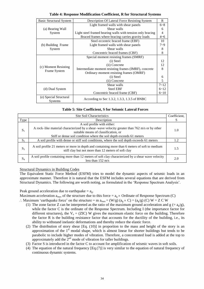
(1) Design Base Shear
The total design base shear in a given direction is determined from the following relation:
V = (ZIC/R) W ……………(5)
where, Z = Seismic zone coefficient given in Table 6.2.22 and Fig. 6.2.10 (BNBC 1993);
i.e., Z = 0.075, 0.15 and 0.25 for Seismic Zones 1, 2 and 3 respectively
I = Structure importance coefficient given in Table 6.2.23, similar to CI for wind
R = Response modification coefficient for structural systems given in Table 4;
i.e., 6.2.24 in BNBC
W = The total seismic dead load
The ‘Seismic Dead Load’ is not only the dead load (including permanent partitions) of the structure but also
has to include some live loads as and when they superimpose on the dead loads.
C = Numerical coefficient given by the relation:
C = 1.25 S/T2/3
…..………………(6)
S = Site coefficient for soil characteristics as provided in Table 5; i.e., 6.2.25 in BNBC
T = Fundamental period of vibration of the structure in the direction considered (in sec)
The value of C need not exceed 2.75. Except for those requirements where Code prescribed forces are scaled
up by 0.375R, the minimum value of the ratio C/R is 0.075.
(2) Structural Period
The value of T may be approximated by the equation T = Ct (hn)3/4
…………….(7)
where, Ct = 0.083 for steel moment resisting frames
= 0.073 for RCC moment resisting frames, and eccentric braced steel frames
= 0.049 for all other structural systems
hn = Height (in meters) above the base to level n.
There are alternative ways of calculating T and Ct.
(3) Vertical Distribution of Lateral Forces
In the absence of a more rigorous procedure, the total lateral force which is the base shear V, is distributed
along the height of the structure in accordance with Eqs. (8)~(10).
V = Ft + Fi …..………(8)
where, Fi = Lateral force applied at storey level i and
Ft = Additional concentrated lateral force considered at the top of the building
The concentrated force, Ft acting at the top of the building is determined as follows:
Ft = 0.07 TV 0.25V when T > 0.7 second, and = 0, when T 0.7 second .…………(9)
The remaining portion of the base shear (V–Ft), is distributed over the height of the building, including level
n, according to the relation
Fj = (V–Ft) [wj hj/wi hi] …...…..…..(10)
The design story shear Vx in any story x is the sum of the forces Fx and Ft above that story.
34
Table 4: Response Modification Coefficient, R for Structural Systems
Basic Structural System Description Of Lateral Force Resisting System R
(a) Bearing Wall
System
Light framed walls with shear panels
Shear walls
Light steel framed bearing walls with tension only bracing
Braced frames where bracing carries gravity loads
6~8
6
4
4~6
(b) Building Frame
System
Steel eccentric braced frame (EBF)
Light framed walls with shear panels
Shear walls
Concentric braced frames (CBF)
10
7~9
8
8
(c) Moment Resisting
Frame System
Special moment resisting frames (SMRF)
(i) Steel
(ii) Concrete
Intermediate moment resisting frames (IMRF), concrete
Ordinary moment resisting frames (OMRF)
(i) Steel
(ii) Concrete
12
12
8
6
5
(d) Dual System
Shear walls
Steel EBF
Concentric braced frame (CBF)
7~12
6~12
6~10
(e) Special Structural
Systems According to Sec 1.3.2, 1.3.3, 1.3.5 of BNBC
Table 5: Site Coefficient, S for Seismic Lateral Forces
Site Soil Characteristics Coefficient,
S Type Description
S1
A soil profile with either:
A rock–like material characterized by a shear–wave velocity greater than 762 m/s or by other
suitable means of classification, or
Stiff or dense soil condition where the soil depth exceeds 61 meters
1.0
S2 A soil profile with dense or stiff soil conditions, where the soil depth exceeds 61 meters 1.2
S3 A soil profile 21 meters or more in depth and containing more than 6 meters of soft to medium
stiff clay but not more than 12 meters of soft clay
1.5
S4 A soil profile containing more than 12 meters of soft clay characterized by a shear wave velocity
less than 152 m/s 2.0
Structural Dynamics in Building Codes
The Equivalent Static Force Method (ESFM) tries to model the dynamic aspects of seismic loads in an
approximate manner. Therefore it is natural that the ESFM includes several equations that are derived from
Structural Dynamics. The following are worth noting, as formulated in the ‘Response Spectrum Analysis’.
Peak ground acceleration due to earthquake = ag.
Maximum acceleration amax of the structure due to this force = ag Ordinate of Response Spectrum (C)
Maximum ‘earthquake force’ on the structure = m amax = (W/g) (ag C) = (ag/g) (C) W = Z C W
(1) The zone factor Z can be interpreted as the ratio of the maximum ground acceleration and g (= ag/g),
while the factor C is the ordinate of the Response Spectrum. Including I (the importance factor for
different structures), the Ve = (ZIC) W gives the maximum elastic force on the building. Therefore
the factor R is the building resistance factor that accounts for the ductility of the building, i.e., its
ability to withstand inelastic deformations and thereby reduce the elastic force.
(2) The distribution of story shear [Eq. (10)] in proportion to the mass and height of the story is an
approximation of the 1st modal shape, which is almost linear for shorter buildings but tends to be
parabolic to include higher modes of vibration. Therefore, a concentrated load is added at the top to
approximately add the 2nd
mode of vibration for taller buildings.
(3) Factor S is introduced in the factor C to account for amplification of seismic waves in soft soils.
(4) The equation of the natural frequency [Eq.(7)] is very similar to the equation of natural frequency of
continuous dynamic systems.
35
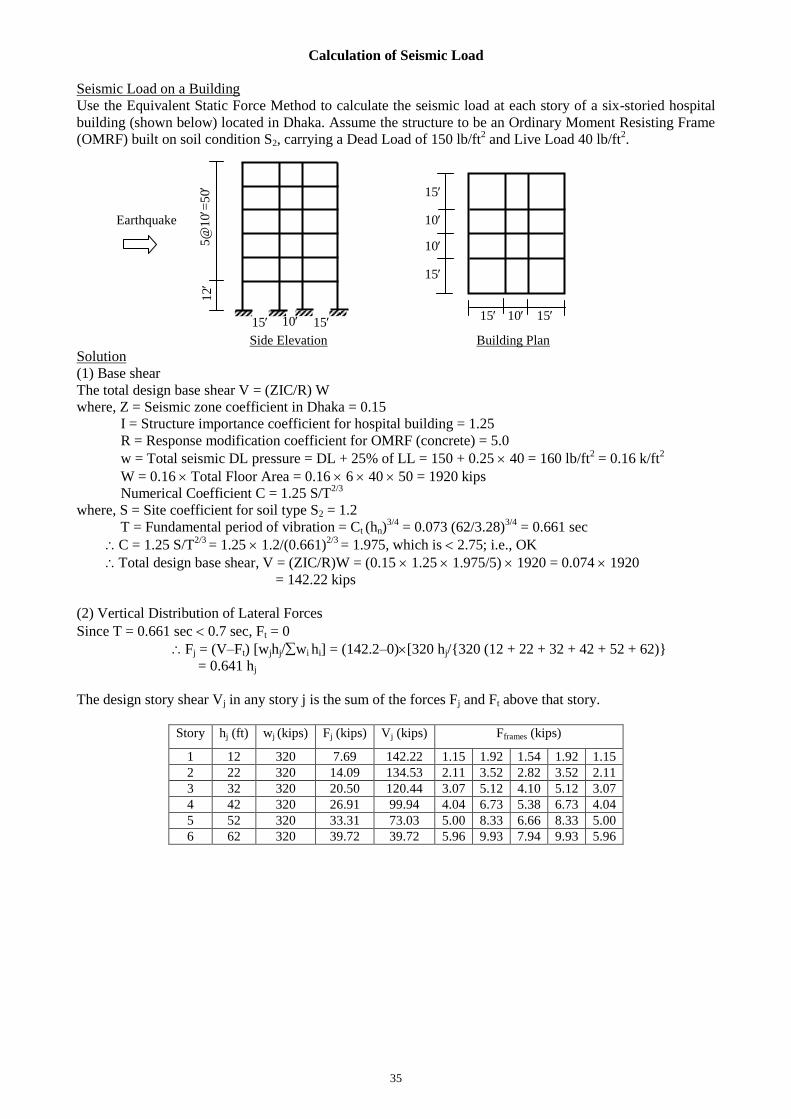
Calculation of Seismic Load
Seismic Load on a Building
Use the Equivalent Static Force Method to calculate the seismic load at each story of a six-storied hospital
building (shown below) located in Dhaka. Assume the structure to be an Ordinary Moment Resisting Frame
(OMRF) built on soil condition S2, carrying a Dead Load of 150 lb/ft2 and Live Load 40 lb/ft
2.
Side Elevation Building Plan
Solution
(1) Base shear
The total design base shear V = (ZIC/R) W
where, Z = Seismic zone coefficient in Dhaka = 0.15
I = Structure importance coefficient for hospital building = 1.25
R = Response modification coefficient for OMRF (concrete) = 5.0
w = Total seismic DL pressure = DL + 25% of LL = 150 + 0.25 40 = 160 lb/ft2 = 0.16 k/ft
2
W = 0.16 Total Floor Area = 0.16 6 40 50 = 1920 kips
Numerical Coefficient C = 1.25 S/T2/3
where, S = Site coefficient for soil type S2 = 1.2
T = Fundamental period of vibration = Ct (hn)3/4
= 0.073 (62/3.28)3/4
= 0.661 sec
C = 1.25 S/T2/3
= 1.25 1.2/(0.661)2/3
= 1.975, which is 2.75; i.e., OK
Total design base shear, V = (ZIC/R)W = (0.15 1.25 1.975/5) 1920 = 0.074 1920
= 142.22 kips
(2) Vertical Distribution of Lateral Forces
Since T = 0.661 sec 0.7 sec, Ft = 0
Fj = (V–Ft) [wjhj/wi hi] = (142.2–0)[320 hj/{320 (12 + 22 + 32 + 42 + 52 + 62)}
= 0.641 hj
The design story shear Vj in any story j is the sum of the forces Fj and Ft above that story.
Story hj (ft) wj (kips) Fj (kips) Vj (kips) Fframes (kips)
1 12 320 7.69 142.22 1.15 1.92 1.54 1.92 1.15
2 22 320 14.09 134.53 2.11 3.52 2.82 3.52 2.11
3 32 320 20.50 120.44 3.07 5.12 4.10 5.12 3.07
4 42 320 26.91 99.94 4.04 6.73 5.38 6.73 4.04
5 52 320 33.31 73.03 5.00 8.33 6.66 8.33 5.00
6 62 320 39.72 39.72 5.96 9.93 7.94 9.93 5.96
5@
10=
50
12
15
10
15
10 15 15
10
15
15
10
Earthquake
36
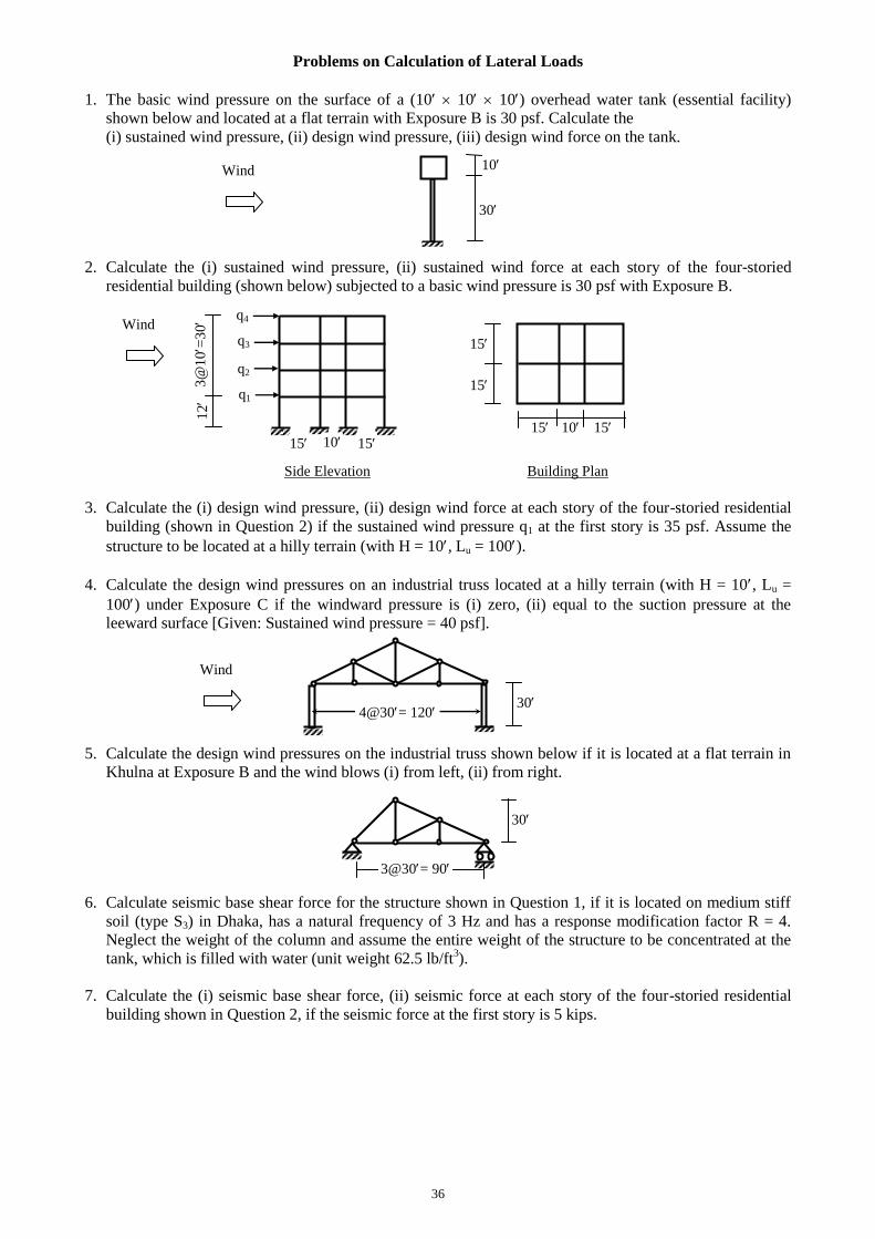
Problems on Calculation of Lateral Loads
1. The basic wind pressure on the surface of a (10 10 10) overhead water tank (essential facility)
shown below and located at a flat terrain with Exposure B is 30 psf. Calculate the
(i) sustained wind pressure, (ii) design wind pressure, (iii) design wind force on the tank.
2. Calculate the (i) sustained wind pressure, (ii) sustained wind force at each story of the four-storied
residential building (shown below) subjected to a basic wind pressure is 30 psf with Exposure B.
Side Elevation Building Plan
3. Calculate the (i) design wind pressure, (ii) design wind force at each story of the four-storied residential
building (shown in Question 2) if the sustained wind pressure q1 at the first story is 35 psf. Assume the
structure to be located at a hilly terrain (with H = 10, Lu = 100).
4. Calculate the design wind pressures on an industrial truss located at a hilly terrain (with H = 10, Lu =
100) under Exposure C if the windward pressure is (i) zero, (ii) equal to the suction pressure at the
leeward surface [Given: Sustained wind pressure = 40 psf].
5. Calculate the design wind pressures on the industrial truss shown below if it is located at a flat terrain in
Khulna at Exposure B and the wind blows (i) from left, (ii) from right.
6. Calculate seismic base shear force for the structure shown in Question 1, if it is located on medium stiff
soil (type S3) in Dhaka, has a natural frequency of 3 Hz and has a response modification factor R = 4.
Neglect the weight of the column and assume the entire weight of the structure to be concentrated at the
tank, which is filled with water (unit weight 62.5 lb/ft3).
7. Calculate the (i) seismic base shear force, (ii) seismic force at each story of the four-storied residential
building shown in Question 2, if the seismic force at the first story is 5 kips.
15
15
12
15
10
15
Wind q3
q2
q1
3@
10=
30 q4
10 15 15
30
10 Wind
30
Wind
4@30= 120
3@30= 90
30
37
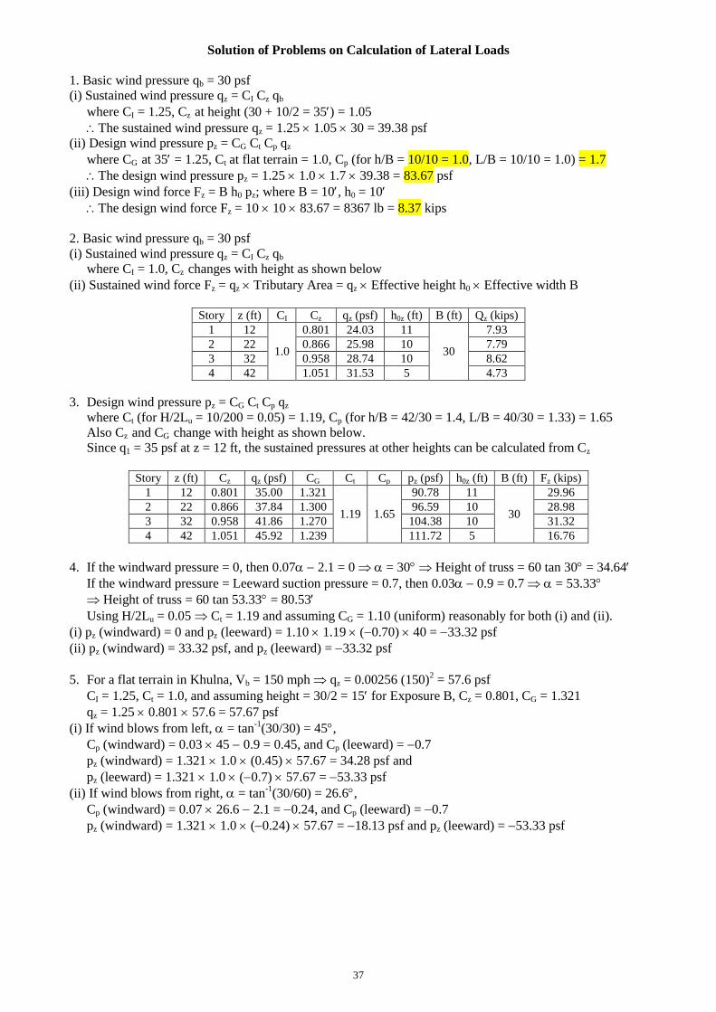
Solution of Problems on Calculation of Lateral Loads
1. Basic wind pressure qb = 30 psf
(i) Sustained wind pressure qz = CI Cz qb
where CI = 1.25, Cz at height (30 + 10/2 = 35) = 1.05
The sustained wind pressure qz = 1.25 1.05 30 = 39.38 psf
(ii) Design wind pressure pz = CG Ct Cp qz
where CG at 35 = 1.25, Ct at flat terrain = 1.0, Cp (for h/B = 10/10 = 1.0, L/B = 10/10 = 1.0) = 1.7
The design wind pressure pz = 1.25 1.0 1.7 39.38 = 83.67 psf
(iii) Design wind force Fz = B h0 pz; where B = 10, h0 = 10
The design wind force Fz = 10 10 83.67 = 8367 lb = 8.37 kips
2. Basic wind pressure qb = 30 psf
(i) Sustained wind pressure qz = CI Cz qb
where CI = 1.0, Cz changes with height as shown below
(ii) Sustained wind force Fz = qz Tributary Area = qz Effective height h0 Effective width B
Story z (ft) CI Cz qz (psf) h0z (ft) B (ft) Qz (kips)
1 12
1.0
0.801 24.03 11
30
7.93
2 22 0.866 25.98 10 7.79
3 32 0.958 28.74 10 8.62
4 42 1.051 31.53 5 4.73
3. Design wind pressure pz = CG Ct Cp qz
where Ct (for H/2Lu = 10/200 = 0.05) = 1.19, Cp (for h/B = 42/30 = 1.4, L/B = 40/30 = 1.33) = 1.65
Also Cz and CG change with height as shown below.
Since q1 = 35 psf at z = 12 ft, the sustained pressures at other heights can be calculated from Cz
Story z (ft) Cz qz (psf) CG Ct Cp pz (psf) h0z (ft) B (ft) Fz (kips)
1 12 0.801 35.00 1.321
1.19 1.65
90.78 11
30
29.96
2 22 0.866 37.84 1.300 96.59 10 28.98
3 32 0.958 41.86 1.270 104.38 10 31.32
4 42 1.051 45.92 1.239 111.72 5 16.76
4. If the windward pressure = 0, then 0.07 2.1 = 0 = 30 Height of truss = 60 tan 30 = 34.64
If the windward pressure = Leeward suction pressure = 0.7, then 0.03 0.9 = 0.7 = 53.33
Height of truss = 60 tan 53.33 = 80.53
Using H/2Lu = 0.05 Ct = 1.19 and assuming CG = 1.10 (uniform) reasonably for both (i) and (ii).
(i) pz (windward) = 0 and pz (leeward) = 1.10 1.19 (0.70) 40 = 33.32 psf
(ii) pz (windward) = 33.32 psf, and pz (leeward) = 33.32 psf
5. For a flat terrain in Khulna, Vb = 150 mph qz = 0.00256 (150)2 = 57.6 psf
CI = 1.25, Ct = 1.0, and assuming height = 30/2 = 15 for Exposure B, Cz = 0.801, CG = 1.321
qz = 1.25 0.801 57.6 = 57.67 psf
(i) If wind blows from left, = tan-1
(30/30) = 45,
Cp (windward) = 0.03 45 0.9 = 0.45, and Cp (leeward) = 0.7
pz (windward) = 1.321 1.0 (0.45) 57.67 = 34.28 psf and
pz (leeward) = 1.321 1.0 (0.7) 57.67 = 53.33 psf
(ii) If wind blows from right, = tan-1
(30/60) = 26.6,
Cp (windward) = 0.07 26.6 2.1 = 0.24, and Cp (leeward) = 0.7
pz (windward) = 1.321 1.0 (0.24) 57.67 = 18.13 psf and pz (leeward) = 53.33 psf

38
6. For an essential structure in Dhaka, Z = 0.15, I = 1.25
Also natural frequency fn = 3 Hz Time period T = 1/3 = 0.33 sec
For soil type S3, S = 1.5 C = 1.25 S/T2/3
= 1.25 1.5/0.332/3
= 3.90 2.75; i.e., C = 2.75
Also response modification factor R = 4.0
Neglecting the weight of the column and tank and considering the weight of water only,
The total seismic weight W = 10 10 10 62.5/1000 = 62.5 kips
Seismic base shear force V = (ZIC/R) W = (0.15 1.25 2.75/4.0) 62.5 = 8.06 kips
7. The seismic force distribution is given by the equation, V = Ft + Fi
where, Fi = Lateral force applied at storey level i, and
Ft = Additional concentrated lateral force considered at the top of the building
Here, T = Fundamental period of vibration = Ct (hn)3/4
= 0.073 (42/3.28)3/4
= 0.49 sec 0.70 sec
Ft = 0
Fj = V [wj hj/wi hi] = V hj/ hi, if floor weights are assumed constant
Seismic forces are assumed to be proportional to height from base
F1 = 5 k F2 = 5 22/12 = 9.17
k, F3 = 5 32/12 = 13.33
k, F4 = 5 42/12 = 17.50
k
Base shear force V = F1 + F2 + F3 + F4 = 5 + 9.17 + 13.33 + 17.50 = 45.0 kips
39
Dynamic Force, Dynamic System and Equation of Motion
Dynamic Force and System
Time-varying loads are called dynamic loads. Structural dead loads and live loads have the same magnitude
and direction throughout their application and are thus static loads. However there are several examples of
forces that vary with time, i.e., those caused by wind, vortex, water wave, vehicle, blast or ground motion.
A dynamic system is a simple representation of physical systems and is modeled by mass, damping and
stiffness. Stiffness is the resistance it provides to deformations, mass is the matter it contains and damping
represents its ability to decrease its own motion with time. A dynamic system resists external forces by a
combination of forces due to its stiffness (spring force), damping (viscous force) and mass (inertia force).
Formulation of the Single-Degree-of-Freedom (SDOF) Equation
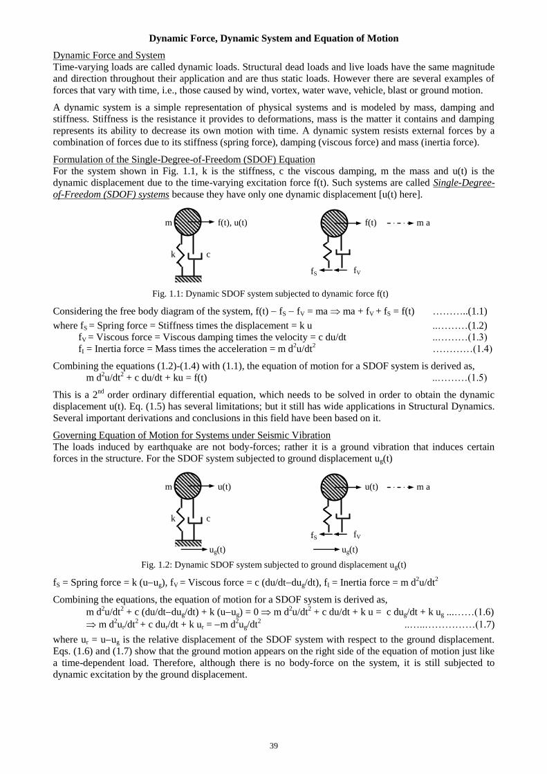
For the system shown in Fig. 1.1, k is the stiffness, c the viscous damping, m the mass and u(t) is the
dynamic displacement due to the time-varying excitation force f(t). Such systems are called Single-Degree-
of-Freedom (SDOF) systems because they have only one dynamic displacement [u(t) here].
m f(t), u(t) f(t)
k c
Fig. 1.1: Dynamic SDOF system subjected to dynamic force f(t)
Considering the free body diagram of the system, f(t) fS fV = ma ma + fV + fS = f(t) ………..(1.1)
where fS = Spring force = Stiffness times the displacement = k u ..………(1.2)
fV = Viscous force = Viscous damping times the velocity = c du/dt ..………(1.3)
fI = Inertia force = Mass times the acceleration = m d2u/dt
2 …………(1.4)
Combining the equations (1.2)-(1.4) with (1.1), the equation of motion for a SDOF system is derived as,
m d2u/dt
2 + c du/dt + ku = f(t) ..………(1.5)
This is a 2nd
order ordinary differential equation, which needs to be solved in order to obtain the dynamic
displacement u(t). Eq. (1.5) has several limitations; but it still has wide applications in Structural Dynamics.
Several important derivations and conclusions in this field have been based on it.
Governing Equation of Motion for Systems under Seismic Vibration
The loads induced by earthquake are not body-forces; rather it is a ground vibration that induces certain
forces in the structure. For the SDOF system subjected to ground displacement ug(t)
m u(t) u(t)
k c
Fig. 1.2: Dynamic SDOF system subjected to ground displacement ug(t)
fS = Spring force = k (uug), fV = Viscous force = c (du/dtdug/dt), fI = Inertia force = m d2u/dt
2
Combining the equations, the equation of motion for a SDOF system is derived as,
m d2u/dt
2 + c (du/dtdug/dt) + k (uug) = 0 m d
2u/dt
2 + c du/dt + k u = c dug/dt + k ug ...……(1.6)
m d2ur/dt
2 + c dur/dt + k ur = m d
2ug/dt
2 ..…..……………(1.7)
where ur = uug is the relative displacement of the SDOF system with respect to the ground displacement.
Eqs. (1.6) and (1.7) show that the ground motion appears on the right side of the equation of motion just like
a time-dependent load. Therefore, although there is no body-force on the system, it is still subjected to
dynamic excitation by the ground displacement.
fS fV
m a
fS fV
m a
ug(t) ug(t)
40
Free Vibration of Damped Systems
As mentioned in the previous section, the equation of motion of a dynamic system with mass (m), linear
viscous damping (c) & stiffness (k) undergoing free vibration is,
m d2u/dt
2 + c du/dt + ku = 0 …………………(1.5)
d2u/dt
2 + (c/m) du/dt + (k/m) u = 0 d
2u/dt
2 + 2n du/dt + n
2 u = 0 …...…..…………(2.1)
where n = (k/m), is the Natural Frequency of the system ...……..…………(2.2)
and = c/(2mn) = cn/(2k) = c/2(km), is the Damping Ratio of the system ...…………….…(2.3)
If 1, the system is called an Underdamped System. Practically, most structural systems are underdamped.
The displacement u(t) for such a system is
u(t) = ent
[C1 cos (dt) + C2 sin (dt)] ...………………(2.4)
where d = n(12) is called the Damped Natural Frequency of the system ………………...(2.5)
If u(0) = u0 and v(0) = v0, then the equation for free vibration of a damped system is given by
u(t) = ent
[u0 cos (dt) + {(v0 + nu0)/d} sin (dt)] ……………...(2.6)
Eq (2.6) The system vibrates at its damped natural frequency (i.e., a frequency of d radian/sec).
Since d [= n(12)] is less than n, the system vibrates more slowly than the undamped system.
Moreover, due to the exponential term ent
, the amplitude of the motion of an underdamped system
decreases steadily, and reaches zero after (a hypothetical) ‘infinite’ time of vibration.
Example 2.1
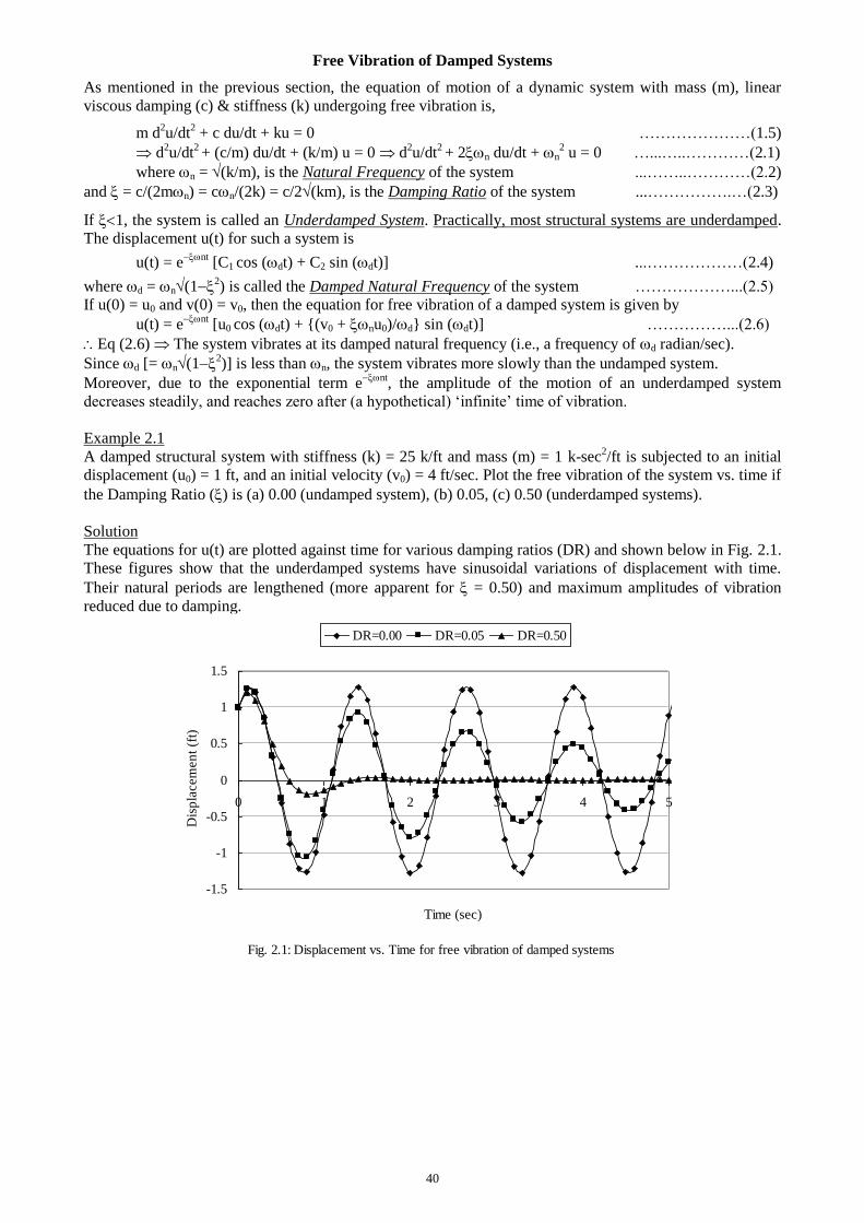
A damped structural system with stiffness (k) = 25 k/ft and mass (m) = 1 k-sec2/ft is subjected to an initial
displacement (u0) = 1 ft, and an initial velocity (v0) = 4 ft/sec. Plot the free vibration of the system vs. time if
the Damping Ratio () is (a) 0.00 (undamped system), (b) 0.05, (c) 0.50 (underdamped systems).
Solution
The equations for u(t) are plotted against time for various damping ratios (DR) and shown below in Fig. 2.1.
These figures show that the underdamped systems have sinusoidal variations of displacement with time.
Their natural periods are lengthened (more apparent for = 0.50) and maximum amplitudes of vibration
reduced due to damping.
Fig. 2.1: Displacement vs. Time for free vibration of damped systems
-1.5
-1
-0.5
0
0.5
1
1.5
0 1 2 3 4 5
Time (sec)
Dis
pla
cem
en
t (f
t)
DR=0.00 DR=0.05 DR=0.50
41
Damping of Structures
Damping is the element that causes impedance of motion in a structural system. There are several sources of
damping in a dynamic system. It can be due to internal resistance to motion between layers, friction between
different materials or different parts of the structure (called frictional damping), drag between fluids or
structures flowing past each other, etc. Sometimes, external forces themselves can contribute to (increase or
decrease) the damping. Damping is also increased in structures artificially by external sources like dampers
acting as control systems.
Viscous Damping of SDOF systems
Linear viscous damping is the most used damping and provides a force directly proportional to the structural
velocity. This is a fair representation of structural damping in many cases and is often convenient to assume
for the purpose of analysis. Viscous damping is usually an intrinsic property of the material and originates
from internal resistance to motion between different layers within the material itself.
The free vibration response of SDOF system with linear viscous damping was found to be
u(t) = e-nt
[u0 cos (dt) + {(v0 + nu0)/d} sin (dt)] ………………..(2.6)
Therefore the displacement at N time periods (Td = 2/d) later than u(t) is
u(t+NTd) = e-n(t+2N/d)
[u0 cos(dt+2N) + {(v0 + nu0)/d} sin(dt+2N)] = e-n(2N/d)
u(t) ..(2.7)
From which, using d = n(1-2) /(1-
2) = ln[u(t)/u(t +NTd)]/2N = = /(1+
2) ...…...…(2.8)
For lightly damped structures (i.e., 1), = ln[u(t)/u(t +NTd)]/2N ..…..……….(2.9)
For example, if the free vibration amplitude of a SDOF system decays from 1.5 to 0.5 in 3 cycles
= ln(1.5/0.5)/(23) = 0.0583 = 5.83%
The damping ratio, = /(1+2) = 0.0582 = 5.82%
Table 2.1: Recommended Damping Ratios for different Structural Elements
Stress Level Type and Condition of Structure (%)
Working stress
Welded steel, pre-stressed concrete, RCC with slight cracking 2-3
RCC with considerable cracking 3-5
Bolted/riveted steel or timber 5-7
Yield stress
Welded steel, pre-stressed concrete 2-3
RCC 7-10
Bolted/riveted steel or timber 10-15
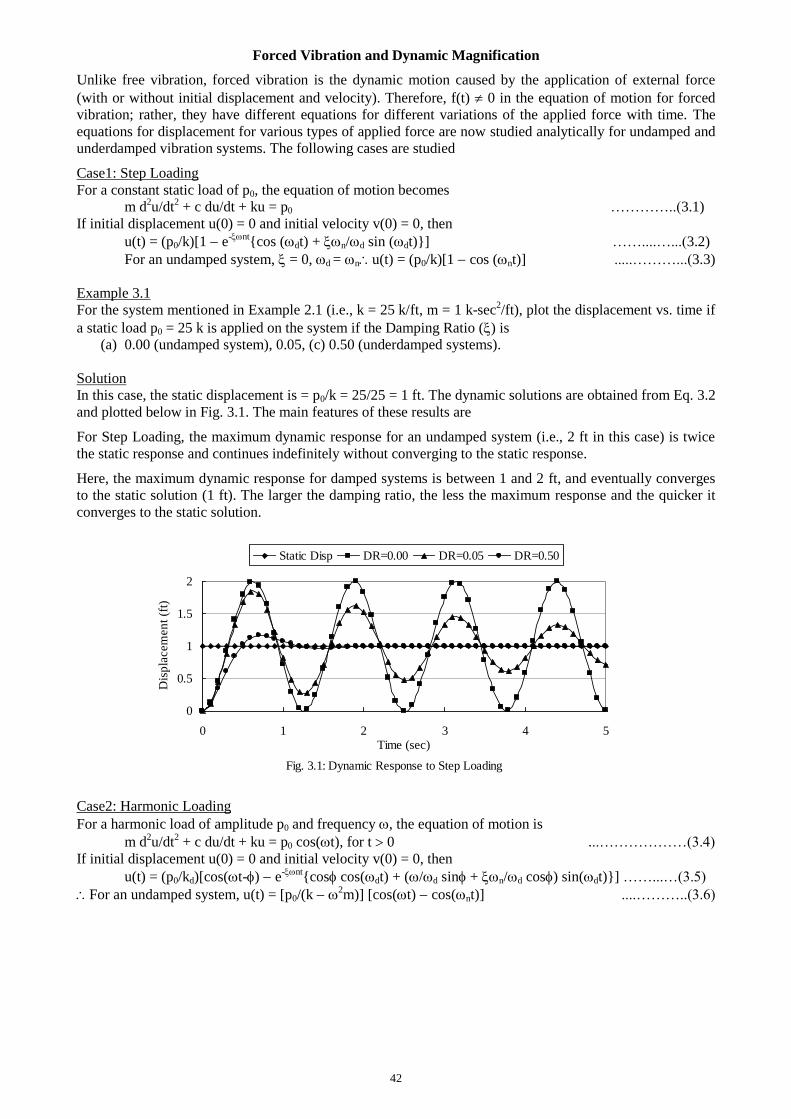
42
Forced Vibration and Dynamic Magnification
Unlike free vibration, forced vibration is the dynamic motion caused by the application of external force
(with or without initial displacement and velocity). Therefore, f(t) 0 in the equation of motion for forced
vibration; rather, they have different equations for different variations of the applied force with time. The
equations for displacement for various types of applied force are now studied analytically for undamped and
underdamped vibration systems. The following cases are studied
Case1: Step Loading
For a constant static load of p0, the equation of motion becomes
m d2u/dt
2 + c du/dt + ku = p0 …………..(3.1)
If initial displacement u(0) = 0 and initial velocity v(0) = 0, then
u(t) = (p0/k)[1 e-nt
{cos (dt) + n/d sin (dt)}] ……....…...(3.2)
For an undamped system, = 0, d = nu(t) = (p0/k)[1 cos (nt)] .....………...(3.3)
Example 3.1
For the system mentioned in Example 2.1 (i.e., k = 25 k/ft, m = 1 k-sec2/ft), plot the displacement vs. time if
a static load p0 = 25 k is applied on the system if the Damping Ratio () is
(a) 0.00 (undamped system), 0.05, (c) 0.50 (underdamped systems).
Solution
In this case, the static displacement is = p0/k = 25/25 = 1 ft. The dynamic solutions are obtained from Eq. 3.2
and plotted below in Fig. 3.1. The main features of these results are
For Step Loading, the maximum dynamic response for an undamped system (i.e., 2 ft in this case) is twice
the static response and continues indefinitely without converging to the static response.
Here, the maximum dynamic response for damped systems is between 1 and 2 ft, and eventually converges
to the static solution (1 ft). The larger the damping ratio, the less the maximum response and the quicker it
converges to the static solution.
Case2: Harmonic Loading
For a harmonic load of amplitude p0 and frequency , the equation of motion is
m d2u/dt
2 + c du/dt + ku = p0 cos(t), for t 0 ...………………(3.4)
If initial displacement u(0) = 0 and initial velocity v(0) = 0, then
u(t) = (p0/kd)[cos(t-) e-nt
{cos cos(dt) + (/d sin + n/d cos) sin(dt)}] ……...…(3.5)
For an undamped system, u(t) = [p0/(k 2m)] [cos(t) cos(nt)] ....………..(3.6)
Fig. 3.1: Dynamic Response to Step Loading
0
0.5
1
1.5
2
0 1 2 3 4 5Time (sec)
Dis
pla
cem
en
t (f
t)
Static Disp DR=0.00 DR=0.05 DR=0.50

43
Dynamic Magnification
If the motion of a SDOF system subjected to harmonic loading is allowed to continue for long (theoretically
infinite) durations, the total response converges to the steady state solution given by the particular solution
of the equation of motion.
usteady(t) = up(t) = (p0/kd) cos(t) ……………..…(3.5)
[where kd = {(k2m)
2 + (c)
2}, = tan
-1{(c)/ (k
2m)}]
Putting the value of kd in Eq. (3.5), the amplitude of steady vibration is found to be
uamplitude = p0/kd = p0/{(k2m)
2 + (c)
2} .……………..….(3.8)
Using ustatic = p0/k uamplitude/ustatic = 1/{(12/n
2)
2 + (2/n)
2} ………...….……(3.9)
Eq. (3.9) gives the ratio of the dynamic and static amplitude of motion as a function of frequency (as well
as structural properties like n and ). This ratio is called the steady state dynamic magnification factor
(DMF) for harmonic motion. Putting the frequency ratio /n = r, Eq. (3.9) can be rewritten as
DMF = 1/{(1r2)
2 + (2r)
2} ………………(3.10)
From which the maximum value of DMF is found = (1/2)/(12), when r = (12
2) …………....(3.11)
The variation of the steady state dynamic magnification factor (DMF) with frequency ratio (r = /n) is
shown in Fig. 3.2 for different values of (= DR). The main features of this graph are
1. The curves for the smaller values of show pronounced peaks [1/(2)] at /n 1. This situation is
called Resonance and is characterized by large dynamic amplifications of motion. This situation can be
derived from Eq. (3.10), where 1 DMFmax 1/(42) = (1/2), when r (12
2) = 1.
2. For undamped system, the resonant peak is infinity.
3. Since resonance is such a critical condition from structural point of view, it should be avoided in practical
structures by making it either very stiff (i.e., r1) or very flexible (i.e., r 1) with respect to the frequency
of the expected harmonic load.
4. The resonant condition mentioned in (1) is not applicable for large values of , because the condition of
maxima at r = (122) is meaningless if r is imaginary; i.e., (1/2 =) 0.707. Therefore, another way of
avoiding the critical effects of resonance is by increasing the damping of the system.
Fig. 3.2: Steady State Dynamic Magnification Factor
0
2
4
6
8
10
0 0.5 1 1.5 2 2.5 3
Frequency Ratio
Dy
nam
ic M
ag
nif
icati
on
Facto
r
DR=0.00 DR=0.05 DR=0.20 DR=0.50 DR=1.00
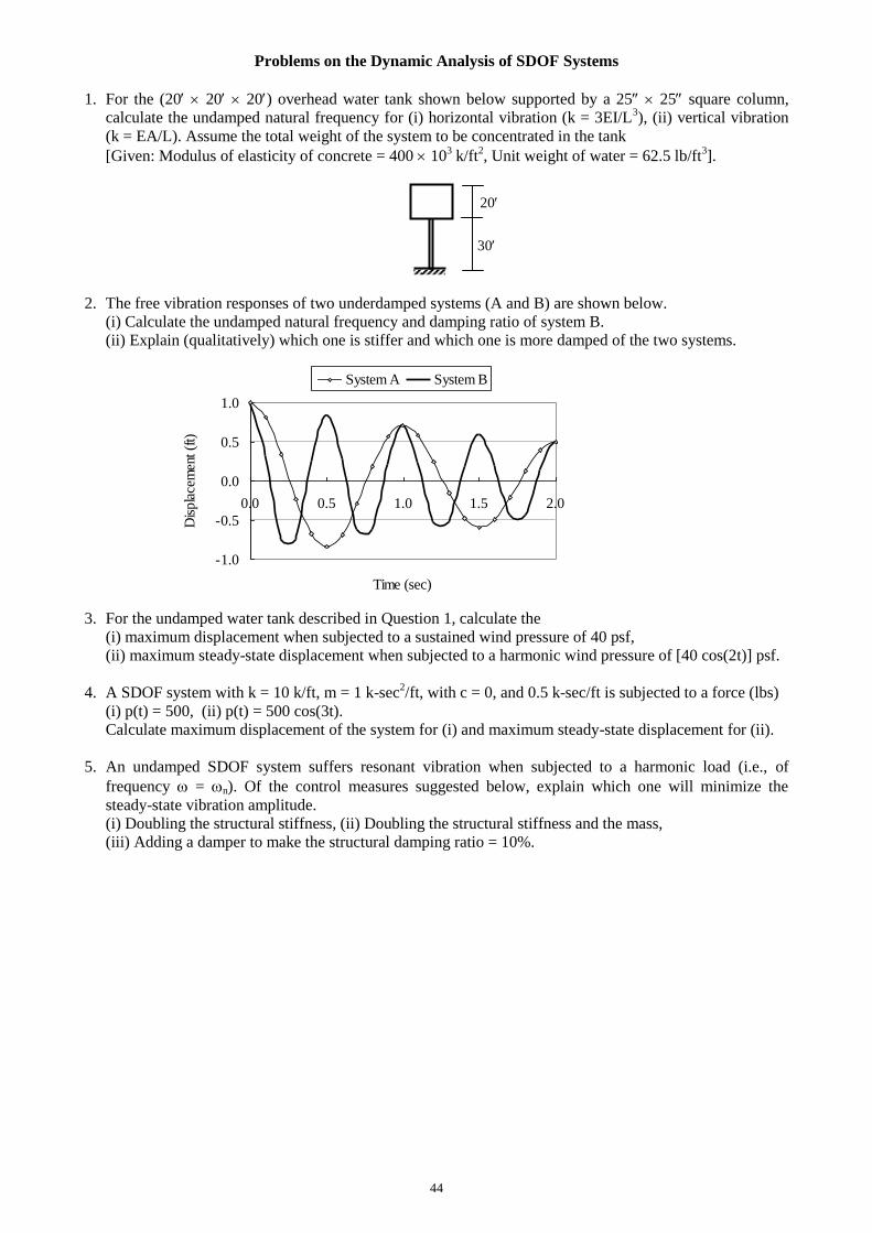
44
Problems on the Dynamic Analysis of SDOF Systems
1. For the (20 20 20) overhead water tank shown below supported by a 25 25 square column,
calculate the undamped natural frequency for (i) horizontal vibration (k = 3EI/L3), (ii) vertical vibration
(k = EA/L). Assume the total weight of the system to be concentrated in the tank
[Given: Modulus of elasticity of concrete = 400 103 k/ft
2, Unit weight of water = 62.5 lb/ft
3].
2. The free vibration responses of two underdamped systems (A and B) are shown below.
(i) Calculate the undamped natural frequency and damping ratio of system B.
(ii) Explain (qualitatively) which one is stiffer and which one is more damped of the two systems.
3. For the undamped water tank described in Question 1, calculate the
(i) maximum displacement when subjected to a sustained wind pressure of 40 psf,
(ii) maximum steady-state displacement when subjected to a harmonic wind pressure of [40 cos(2t)] psf.
4. A SDOF system with k = 10 k/ft, m = 1 k-sec2/ft, with c = 0, and 0.5 k-sec/ft is subjected to a force (lbs)
(i) p(t) = 500, (ii) p(t) = 500 cos(3t).
Calculate maximum displacement of the system for (i) and maximum steady-state displacement for (ii).
5. An undamped SDOF system suffers resonant vibration when subjected to a harmonic load (i.e., of
frequency = n). Of the control measures suggested below, explain which one will minimize the
steady-state vibration amplitude.
(i) Doubling the structural stiffness, (ii) Doubling the structural stiffness and the mass,
(iii) Adding a damper to make the structural damping ratio = 10%.
-1.0
-0.5
0.0
0.5
1.0
0.0 0.5 1.0 1.5 2.0
Time (sec)
Dis
pla
cem
ent (f
t)
System A System B
30
20
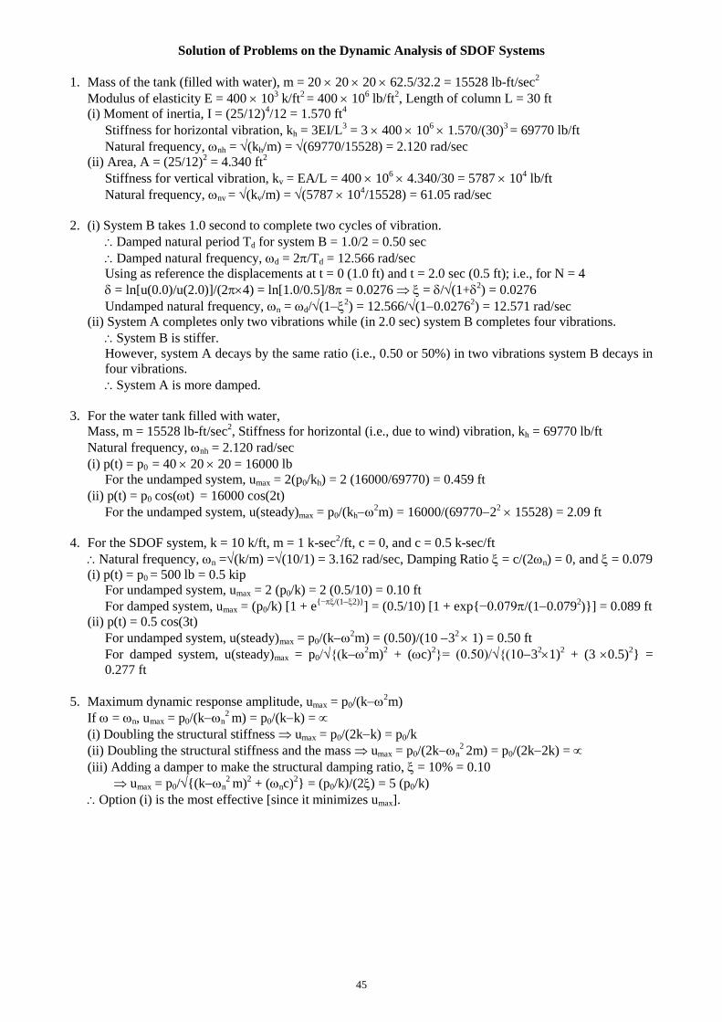
45
Solution of Problems on the Dynamic Analysis of SDOF Systems
1. Mass of the tank (filled with water), m = 20 20 20 62.5/32.2 = 15528 lb-ft/sec2
Modulus of elasticity E = 400 103 k/ft
2 = 400 10
6 lb/ft
2, Length of column L = 30 ft
(i) Moment of inertia, I = (25/12)4/12 = 1.570 ft
4
Stiffness for horizontal vibration, kh = 3EI/L3 = 3 400 10
6 1.570/(30)
3 = 69770 lb/ft
Natural frequency, nh = (kh/m) = (69770/15528) = 2.120 rad/sec
(ii) Area, A = (25/12)2 = 4.340 ft
2
Stiffness for vertical vibration, kv = EA/L = 400 106 4.340/30 = 5787 10
4 lb/ft
Natural frequency, nv = (kv/m) = (5787 104/15528) = 61.05 rad/sec
2. (i) System B takes 1.0 second to complete two cycles of vibration.
Damped natural period Td for system B = 1.0/2 = 0.50 sec
Damped natural frequency, d = 2/Td = 12.566 rad/sec
Using as reference the displacements at t = 0 (1.0 ft) and t = 2.0 sec (0.5 ft); i.e., for N = 4
= ln[u(0.0)/u(2.0)]/(24) = ln[1.0/0.5]/8 = 0.0276 = /(1+2) = 0.0276
Undamped natural frequency, n = d/(12) = 12.566/(10.0276
2) = 12.571 rad/sec
(ii) System A completes only two vibrations while (in 2.0 sec) system B completes four vibrations.
System B is stiffer.
However, system A decays by the same ratio (i.e., 0.50 or 50%) in two vibrations system B decays in
four vibrations.
System A is more damped.
3. For the water tank filled with water,
Mass, m = 15528 lb-ft/sec2, Stiffness for horizontal (i.e., due to wind) vibration, kh = 69770 lb/ft
Natural frequency, nh = 2.120 rad/sec
(i) p(t) = p0 = 40 20 20 = 16000 lb
For the undamped system, umax = 2(p0/kh) = 2 (16000/69770) = 0.459 ft
(ii) p(t) = p0 cos(t) = 16000 cos(2t)
For the undamped system, u(steady)max = p0/(kh2m) = 16000/(697702
2 15528) = 2.09 ft
4. For the SDOF system, k = 10 k/ft, m = 1 k-sec2/ft, c = 0, and c = 0.5 k-sec/ft
Natural frequency, n =(k/m) =(10/1) = 3.162 rad/sec, Damping Ratio = c/(2n) = 0, and = 0.079
(i) p(t) = p0 = 500 lb = 0.5 kip
For undamped system, umax = 2 (p0/k) = 2 (0.5/10) = 0.10 ft
For damped system, umax = (p0/k) [1 + e{−/(12)}
] = (0.5/10) [1 + exp{−0.079/(10.0792)}] = 0.089 ft
(ii) p(t) = 0.5 cos(3t)
For undamped system, u(steady)max = p0/(k2m) = (0.50)/(10 3
2 1) = 0.50 ft
For damped system, u(steady)max = p0/√{(k2m)
2 + (c)
2}= (0.50)/√{(103
21)
2 + (3
0.5)
2} =
0.277 ft
5. Maximum dynamic response amplitude, umax = p0/(k2m)
If = n, umax = p0/(kn2 m) = p0/(kk) =
(i) Doubling the structural stiffness umax = p0/(2kk) = p0/k
(ii) Doubling the structural stiffness and the mass umax = p0/(2kn2 2m) = p0/(2k2k) =
(iii) Adding a damper to make the structural damping ratio, = 10% = 0.10
umax = p0/{(kn2 m)
2 + (nc)
2} = (p0/k)/(2) = 5 (p0/k)
Option (i) is the most effective [since it minimizes umax].

46
Vortex Induced Vibration (VIV)
The pressure difference around a bluff body in flowing fluid may result in separated flow and shear layers
over a large portion of its surface. The outermost shear layers (in contact with the fluid) move faster than the
innermost layers, which are in contact with the structure. If the fluid velocity is large enough, this causes the
shear layers to roll into the near wake and form periodic vortices. The interaction of the structure with these
vortices causes it to vibrate transverse to the flow direction, and this vibration is called VIV.
The frequency of vortex-shedding is called Strouhal frequency (after Strouhal 1878), given by
fs = SU/D ………………(4.1)
where U = Fluid Velocity, D = Transverse dimension (diameter) of the structure, and S = Strouhal number,
which is a function of Reynolds number and the geometry of the structure. For circular cylinders, S 0.20.
Experimental results suggest that VIV usually causes structural vibrations at the frequency fs. However, if fs
is near (about 0.9-1.2 times) the natural frequency (fn) of the structure, the structure vibrates at its natural
frequency. Obviously, this is the most significant feature of VIV and is known as synchronization or lock-in.
For a structure, VIV can be important enough to cause fatigue or instability failure; and over the years it has
been observed in both wind-driven as well as marine structures. The research on the fundamental nature of
VIV has developed in two different directions. One is the rigorous treatment by computational fluid
dynamics using Navier-Stokes equations. Although it has enjoyed success, this approach is still not
developed enough for practical design purposes. The other direction has been primarily aimed at predicting
structural response and modeling the associated fluid-dynamic phenomena by coupled/uncoupled dynamic
equations of motion. Since we primarily aim to predict structural responses due to VIV, and therefore focus
on a simple dynamic model, developed by Iwan and Blevins (1974).
Incorporating experimental results into the equation of motion is equivalent to adding a harmonic load and
an additional damping into the system. The harmonic load has a frequency e s = 2fs, and is similar to
the form
0.5 U2D CL sin (et), where CL 0.50, for several experimental data.
Also, the added damping/length is 0.4 UD ……………….(4.2)
Therefore, for uniform structural dimensions throughout its length L, the dynamic SDOF system is modeled
as
m d2u/dt
2 + (c + 0.4 UDL) du/dt + ku = 0.25 U
2DL sin(st) ..………………(4.3)
Example 4.1
Calculate the dynamic force and added damping due to wind-driven VIV for a cylindrical water tank of 20-
diameter, 20-height and supported by two 30-high concrete columns of 25-diameter each, considering
(i) Design wind speed in Dhaka, (ii) Lock-in phenomenon.
Mass of the tank (filled with water), m = (/4) 202 20 62.5/32.2 = 12196 lb-ft/sec
2
Modulus of elasticity E = 400 106 lb/ft
2, Length of column L = 30 ft
Moment of inertia, I = (25/12)4/64 = 0.925 ft
4
Stiffness for horizontal vibration, kh = 2 3EI/L3 = 82196 lb/ft, Natural frequency, n = 2.60 rad/sec
If U = 130 mph = 190.67 ft/sec, s = 2 (0.2 190.67/20) = 11.98 rad/sec
= Density of air = 0.0765/32.2 = 23.76 10-4
slug/ft3
Dynamic force amplitude = 0.25 U2 DL = 0.25 23.76 10
-4 (190.67)
2 20 20
= 8638 lb
Added damping = 0.4 UDL = 0.4 23.76 10-4 190.67
20 20 =
72.48 lb-sec/ft
Since s/n = 11.98/2.60 = 4.611, VIV is not very important at this velocity.
Lock-in occurs when s = n = 2.60 rad/sec 2 (0.2 U/20) = 2.60 U = 41.32 ft/sec = 28.2 mph
Dynamic force amplitude = 0.25 U2 DL = 0.25 23.76 10
-4 (41.32)
2 20 20
= 405 lb
Added damping cadd = 0.4 UDL = 0.4 23.76 10-4 41.32
20 20 =
15.71 lb-sec/ft
Added damping ratio add = cadd/[2√(km)] = 15.71/[2√(82196 12196)] = 0.00025, which is very small
Therefore, unless the system itself is sufficiently damped, the static deflection of (405/82196 =) 0.0049 ft
will be hugely amplified.
47
Different Types of Dynamic Loads
Hydrodynamic Force
Morison’s equation is easily the most used equation for calculation of hydrodynamic force on
marine/offshore structures. According to the Morison’s equation, the horizontal wave-force on a structure of
height L for a water-depth of d is given by
f(t) = Inertia Force + Drag Force = fI
+ fD .……………(4.4)
For regular waves, the ‘linearized’ force can be calculated (after adjustments for structural acceleration) as
fI (1)
= KI (a2/k)[1− sinh(k(d−L))/sinh(kd)] sin = fI 0 sin () ..……………(4.5)
and fD (1) (4/3KD(a
2[{2kL+sinh(2kd)−sinh(2k(d−L))}/sinh
2 kd] cos cos = fD0 cos cos ……..(4.6)
with additional damping ca (4/3KD(ak)
[1− sinh(k(d−L)/sinh kd] …………….(4.7)
where KI = CIA, KD= CDR, = kx −t +
= Water density, CI = Inertia coefficient, CD = Drag coefficient
A = Cross-sectional area, R = Radius = Half-width of projected surface
ax = Horizontal wave-acceleration, ur = Horizontal (wave velocity – structural velocity)
Vehicular Load
As shown in Fig. 4.1, a wheel load of p0 is traveling with a velocity v over a simply supported beam of
length L. The wheel traveling with a velocity v takes time td = L/v to cross the bridge. Its position at any time
t is as shown in Fig 4.1.
Wheel Load p0, Velocity v
Fig. 4.1: Single wheel on Simply Supported Beam
The moving load can be described mathematically as
f(t) = p0 sin(vt/L), when 0 t td
= 0, when t td ..………………...(4.8)
Blast Loading
According to BNBC, the internal overpressure (q) developed from an internal explosion such as due to leaks
in gas pipes, evaporation of volatile liquids, etc. in typical room sizes may be calculated from the following
time-dependent function
q(t) q0 where q0 is a function of window area and volume of the room
while 0.1 t1 1.0 sec, 1.0 t2 10 sec
Machine Vibrations
The centrifugal force due to vibration of a mass m rotating at an angular velocity and radius r0 that
transfers to a machine foundation can be calculated from
f(t) = m2 r0 sin(t) ………..…..(4.9)
t1 t2 t
48
Wave Force using Morison’s Equation
Morison’s equation is easily the most used equation for calculation of hydrodynamic force on
marine/offshore structures. According to the (modified) Morison’s equation, the horizontal wave-force on a
differential vertical segment dz is given (after adjustments for structural acceleration) by
FI(1)
= KI (a2/k)[1− sinh(k(d−L))/sinh(kd)] sin = FD0 sin ..……………(4.10)
dFx = [KI ax + KD|ur|u] dz ..………………...(4.4)
where KI = CIA, KD= CDR
= Water density, CI = Inertia coefficient, CD = Drag coefficient
A = Cross-sectional area, R = Radius = Half-width of projected surface
ax = Horizontal wave-acceleration, ur = Horizontal (wave velocity – structural velocity)
In equation (4.4), the first term gives the inertia force, and the second is the drag force.
Total horizontal force Fx = dFx, where implies integration between z = −L (bottom of the structure) and z =
(instantaneous wave-elevation).
Once the forces are calculated, the structural dynamic problem can be modeled as
M d2u/dt
2 + C du/dt + k u = Fx ..…………….….(4.5)
However, the mass M is now a combination of the structural mass m and the ‘added’ mass ma. The ‘added’ mass
is obtained from the mathematical adjustment of the equation of motion and is proportional to mass m added by
the mass of water occupying the same volume as the structure. For example, ma for a uniform cylinder is =
R2L
he effective mass, M = m + ma …………………...(4.6)
The damping C is a combination of the structural damping c and the damping ca added from the relative velocity
(drag) term of the load vector, which is obtained from the mathematical adjustment of the equation of motion.
he mass-matrix, C = c + ca …………………...(4.7)
Common values of CI are 2.0 for a cylinder and 1.5 for sphere. However, the drag coefficient CD strongly
depends on the Reynolds number (= uD/); whereas it converges to nearly 0.6-0.7 for high Reynolds
numbers, it can be as high as 3.0 for small Reynolds numbers (i.e., for thinner structural elements like truss
members).
First Order Inertia Force
Integration of the 1st order inertia force over the depth of the structure gives the 1
st order potential force with
FI(1)
= KI (aii2/ki)[1− sinh(ki(d−L))/sinh(kid)] sin i ………………...(4.8)
where, i = ki x −it + i and ‘wave number’ ki can be obtained from i2 = g ki tanh (kid) ....…...…(4.9)
For regular waves, it simplifies to FI(1)
= KI (a2/k)[1− sinh(k(d−L))/sinh(kd)] in = FD0 sin …………(4.10)
First Order (Linearized) Drag
The drag force is given by KD|ur(1)
|u(1)
dz, which can be approximately ‘linearized’. In addition to the drag force
involved, this turns out to be a major contributor to the damping of the system.
For irregular Gaussian waves, the total ‘linearized’ drag force FD(1) 8/ KDur(1) u
dz …....……(4.11)
However for regular waves, the following equation can be used conveniently
FD(1) (4/3KD(a
2[{2kL+sinh(2kd)−sinh(2k(d−L))}/sinh
2 kd] cos cos = FD0 cos cos …..(4.12)
and the additional damping
ca (4/3KD(ak)
[1− sinh(k(d−L)/sinh kd] …………….(4.13)
The maximum hydrodynamic force from Eq. (4.4) is Fmax = √(FI02 + FD0
2) …………….(4.14)
In addition to the inertia and drag forces, a mean drift force acts on the structure that cannot be predicted by
Morison’s equation. However the drag term in Morison’s equation can account for the force (Fc) and damping
(cc) due to uniform current of velocity Uc, the force being given by
Fc KDUc2 L ………………(4.15)
cc KDUc
L ………………(4.16)