strongly correlated systems in atomic and condensed matter...

Strongly correlated systems

in atomic and condensed matter physics

Lecture notes for Physics 284

by Eugene Demler

Harvard University

January 25, 2011

Chapter 6

Bose Hubbard model

6.1 Qualitative arguments

We consider spinless bosonic atoms in an optical lattice with repulsive interac-tion between atoms[11]. They can be described by the Bose Hubbard model[9].

H = −t∑〈ij〉

b†i bj +U

2

∑i

ni (ni − 1)− µ∑i

ni (6.1)

We have on-site interaction only since particles have contact interaction andand we assume tight-binding limit. Away from the tight-binding regime, andespecially for shallower lattices, one may need to include non-local interactions.In the presence of confining potential we also need to include

Hpot =∑i

V (ri)ni (6.2)

Parameters t and U can be controlled by selecting the strength of the opticallattice and tuning the scattering length with magnetic field.

We discuss two limiting cases first.Weak interactions regime t >> U .

Atoms condense into the state of the lowest kinetic energy

|ΨSF〉 =1√N !

(b†k=0)Nat |0〉 ≈ c e√Natb

†k=0 |0〉 (6.3)

Here |0〉 is the vaccum state with no particles. State (6.3) is a superfluid state.We can also write

b†k=0 =1√Nsites

∑i

b†i (6.4)

to write

|ΨSF〉 = c∏i

e

qNatomsNsites

b†i (6.5)

3

4 CHAPTER 6. BOSE HUBBARD MODEL

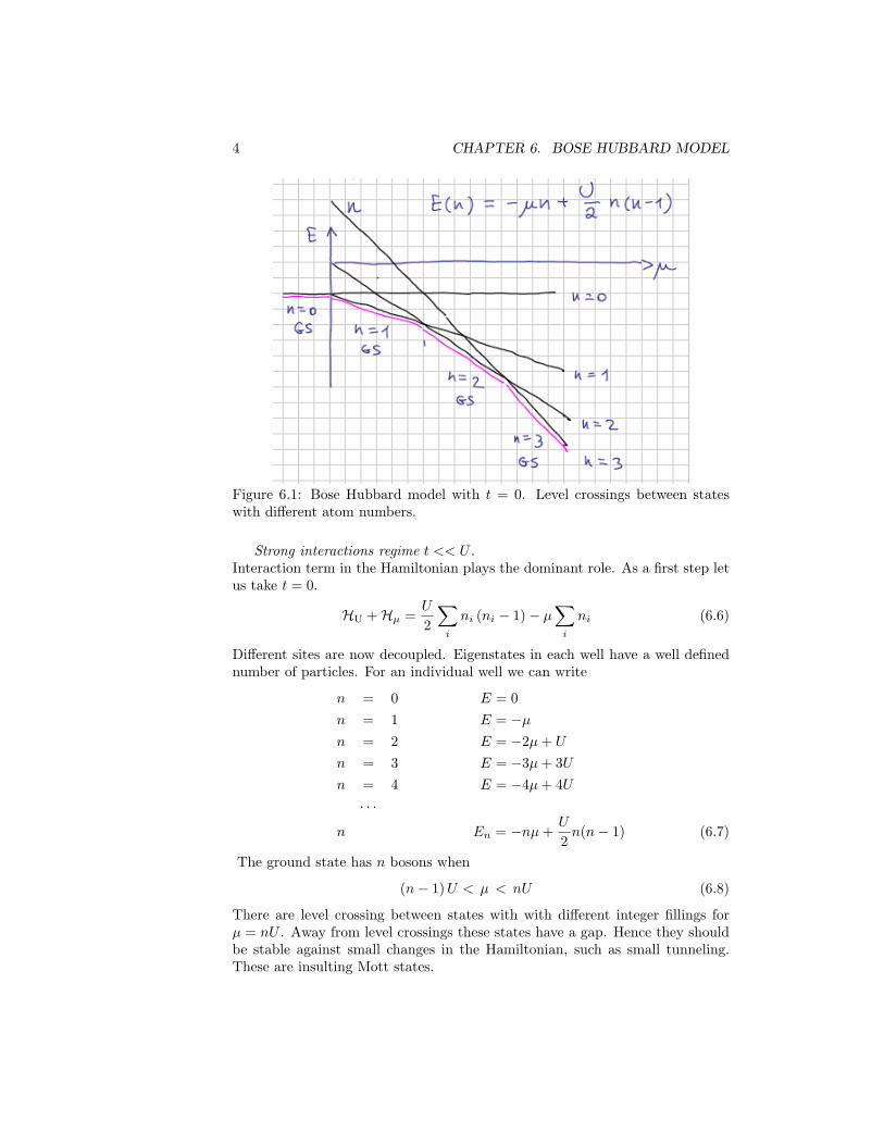
Figure 6.1: Bose Hubbard model with t = 0. Level crossings between stateswith different atom numbers.

Strong interactions regime t << U .Interaction term in the Hamiltonian plays the dominant role. As a first step letus take t = 0.

HU +Hµ =U

2

∑i

ni (ni − 1)− µ∑i

ni (6.6)

Different sites are now decoupled. Eigenstates in each well have a well definednumber of particles. For an individual well we can write

n = 0 E = 0n = 1 E = −µn = 2 E = −2µ+ U

n = 3 E = −3µ+ 3Un = 4 E = −4µ+ 4U· · ·

n En = −nµ+U

2n(n− 1) (6.7)

The ground state has n bosons when

(n− 1)U < µ < nU (6.8)

There are level crossing between states with with different integer fillings forµ = nU . Away from level crossings these states have a gap. Hence they shouldbe stable against small changes in the Hamiltonian, such as small tunneling.These are insulting Mott states.

6.2. GUTZWILLER VARIATIONAL WAVEFUNCTIONS 5

6.2 Gutzwiller variational wavefunctions

To describe transitions between the superfluid and insulating states we useGutzwiller variational wavefunction

|ΨG〉 =∏i

(f0 + f1b

† + f2b† 2i√

2+ · · ·+ fn

b†ni√n!

)|0〉 (6.9)

This wavefunction requires normalization condition∑n

|fn|2 = 1 (6.10)

Our justification for using the Gutzwiller ansatz is that a factorizable wave-function works in both extreme limits: deep in the superfluid state and deep inthe Mott state. It is natural to assume that this wavefunction will work near thetransition point as well. It turns out that this wavefunction is quite accurate ind=3, but in lower dimensions it works only qualitatively. The transition pointobtained from the MC analysis is sufficiently different from the one predictedby the Gutzwiller ansatz. This is not surprising since this is essentially themean-field analysis which becomes increasingly better in higher dimensions.

We need to minimize the wavefunction (6.9) with respect to fn subject tothe constraint (6.10).Interaction energy

〈HU +Hµ〉 = −µ|f1|2 + (2µ+ U)|f2|2 + · · ·+ (−nµ+U

2n(n− 1))|fn|2 + · · ·(6.11)

Kinetic energy

Ht = −zt| f∗0 f1 +√

2f∗1 f2 +√

3f∗2 f3 + · · · |2 (6.12)

Interaction energy favors a fixed number of particles per well, while the kineticenergy favors a coherent superposition of the number states. To understand thetransition let us consider the stability of the Mott state with n particles (at afixed density). We take the Gutzwiller wavefunction with

fn = (1− 2α2)1/2 fn−1 = fn+1 = α (6.13)

here α is assumed to be small and all other fi are zero. We expand the energyup to the second order in α

Ht = −zt|α (1− 2α2)1/2√n+ α (1− 2α2)1/2

√n+ 1 |2 ≈ −ztα2|

√n+√n+ 1|2

(6.14)

We take the middle of the Mott plateau

µ = U(n− 1/2) (6.15)


Figure 6.2: Phase diagram of the Bose Hubbard model according to theGutzwiller variational wavefunction.

We have for the relvant number states

〈HU +Hµ〉n =U

2n(n− 1)− U(n− 1/2)n = −U

2n2

〈HU +Hµ〉n−1 =U

2(n− 1)(n− 2)− U(n− 1/2)(n− 1) = −U

2, (n2 − 1)

〈HU +Hµ〉n+1 =U

2(n− 1)n− U(n− 1/2)(n+ 1) = −U

2, (n2 − 1)(6.16)

Thus we find

Etot(α) = −z tα2 |√n+√n+ 1|2 +

U

22α2 + · · · (6.17)

The Mott to Superfluid transition takes place when the coefficient in front ofα2 becomes negative. For large n this corresponds to

U = 4nzt (6.18)

Note that the Mott state exists only for integer filling factors. For 〈n〉 =N + ε, even when N atoms become localized, ε makes a superfluid state evenfor the smallest values of tunneling.

Confining parabolic potential acts as a cut through the phase diagram.Hence in a parabolic potential we find a ”wedding cake” structure of shells.

6.3. EXPERIMENTS ON THE SUPERFLUID TO MOTT TRANSITION IN OPTICAL LATTICES7

Figure 6.3: Density distribution of atoms in an optical lattice in the Hubbardregime. Incompressible Mott states give rise to the flat plateaus. Compressiblesuperfluid shells make regions where the density is changing smoothly.

6.3 Experiments on the superfluid to Mott tran-sition in optical lattices

Superfluid to Mott insulator transition for ultracold atoms in optical latticeswas first demonstrated by Greiner et al. [1] (see fig. 6.4). They use TOFexperiments to measure occupation numbers in momentum space nk = b†kbk,where k is the physical momentum. In the SF state we have macroscopic occu-pation of the state with the lowest kinetic energy. In a lattice a state with thelowest kinetic energy is a state with quasi-momentum zero. Quasi-momentumdiffers from the physical momentum by Bragg reflections. So in the SF stateatoms should exhibit macroscopic occupation of states with momenta equal toreciprocal lattice vectors. One can also understand this result as constructiveinterference from a periodic array of coherent sources. Finite size of wavefunc-tions in individual wells determines how many Bragg peaks can be observed.In the Mott state one occupies all quasimomenta so expansion images do nothave sharp peaks. We can also say that we no longer have coherent sources sointerference is lost. There has been a certain controversy regarding finite widthof the peaks. It was suggested that this was due to the high temperature inthe system, thus experiments could not be considered a demonstration of thequantum phase transition. Detailed analysis showed that this can be explainedby the finite TOF expansion time [2].

Considerable effort was also dedicated to observing the ”wedding cake” struc-ture in a parabolic potential. Recent experiments reached single site resolutionand provided convincing demonstration of the incompressible Mott plateaus andthe wedding cake structure [4, 8, 3] (see fig.6.5). Note that these experimentscan be used to measure not only the average number of particles, but also fluc-tuations. In the superfluid state we expect to see much large fluctuations sincethey correspond to a superposition of several number states.


Figure 6.4: Demonstration of the superfluid to insulator transition with bosonsin an optical lattice[1]. These TOF experiments measure occupation numberin momentum space nk = b†kbk. In the superfluid state there is macroscopicoccupation of the state with the lattice quasimomentum equal to zero. In TOFthis shows up as peaks for momenta that correspond to reciprocal lattice vectors.In the Mott state all quasimomenta are occupied.

6.4 Collective modes in Bose Hubbard model

6.4.1 Superfluid state

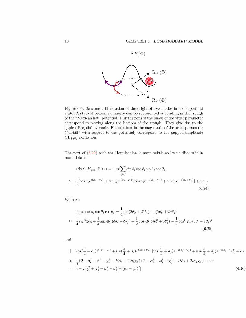
In the superfluid phase we have an order parameter 〈bi〉 = |Φ|eiφ. We ex-pect two types of collective mode: phase fluctuations correspond to gaplessBogoliubov-like excitations. This is the Goldstone mode of the spontaneouslybroken symmetry. Fluctuations of the amplitude of the order parameter corre-spond to a massive Higgs like mode (see fig. 6.6). We discuss simple analysisthat illustrates the appearance of these modes.

We consider a variational wavefunction in which we keep states with n− 1,n , and n+ 1 particles only.

|Ψ〉 =∏i

[e−iχi cos θi

(e−iφi sin( γi ) |n− 1〉 + eiφi cos( γi ) |n+ 1〉

)+ eiχi sin θi |n〉

]i

(6.19)

We are interested in states with the average number of atoms per site n, henceγ should be close to π/4. We introduce γ = π

4 − σ. Truncating the Gutzwillerwavefunction to only three Fock (number) states is a reasonable approximationclose to the superfluid to Mott transition, where number fluctuations are small.For simplicity, we will also assume that n is large so we can neglect the differencebetween n and n± 1.

First we do the mean-field analysis for the wavefunction (6.19).The minimumenergy state requires χ = 0, φ arbitrary but uniform, and σ = 0 when the density

6.4. COLLECTIVE MODES IN BOSE HUBBARD MODEL 9

Figure 6.5: Wedding cake structure in a parabolic potential[3]. In these exper-iments the number of particles in individual wells is measured modulo two. Inother words two particles appear as zero, three particles appear as one. Figuresshow both the average number of particles and the variance. The variance islarge in the superfluid shells.

is precisely n. Energy as a function of θ

E = −nzt2

sin2 θ +U

2cos2 θ (6.20)

Minimizing with respect to θ we find that when U > 4nzt we have a Mott statewith θ = π/2, when U < 4nzt we find a superfluid state with

cos 2θ0 = −U/4nzt (6.21)

Our goal is to project dynamics into the variational state (6.19) and analyzecollective modes. Let us consider the Lagrangian defined as

L = 〈Ψ(t) |(−i) ∂t +H|Ψ(t) 〉 (6.22)

If |Ψ(t) 〉 was arbitrary, by finding an extremum of L with respect to |Ψ(t) 〉 wewould recover the Schroedinger equation. To find projected dynamics we assumethat wavefunctions in (6.22) are limited to the class of wavefunctions describedby equation (6.19) and look for the extremum of L [10, 6]. All parametersin (6.19) are functions of time and can be different at different sites. To findthe extremum of L one can write equations of motion for individual variablesdt∂qi

L = ∂qiL, where qi stands for all variables in (6.19). Since we are interested

in collective modes only, we consider small fluctuations around the euilibriumstate (6.21) and expand up to quadratic order in σi, χi, δθi = θi−θ0. Moreoverwe are interested in the long wavelength behavior of collective modes. Thus ourplan is to get the continuum limit of L first and then write equations of motion.

We have

〈Ψ(t) |(−i) ∂t|Ψ(t) 〉 =∑i

[ cos 2θ0χi − 2 sin 2θ0δθχi + 2 sin2 θ0σφi ] (6.23)


Figure 6.6: Schematic illustration of the origin of two modes in the superfluidstate. A state of broken symmetry can be represented as residing in the troughof the ”Mexican hat” potential. Fluctuations of the phase of the order parametercorrespond to moving along the bottom of the trough. They give rise to thegapless Bogoliubov mode. Fluctuations in the magnitude of the order parameter(”uphill” with respect to the potential) correspond to the gapped amplitude(Higgs) excitation.

The part of (6.22) with the Hamiltonian is more subtle so let us discuss it inmore details

〈Ψ(t) |Hkin|Ψ(t) 〉 = −nt∑〈ij〉

sin θi cos θi sin θj cos θj

×{

[cos γiei(φi−χi) + sin γiei(φi+χi)][cos γje−i(φj−χj) + sin γje−i(φj+χj)] + c.c.}

(6.24)

We have

sin θi cos θi sin θj cos θj =14

sin(2θ0 + 2δθi) sin(2θ0 + 2δθj)

≈ 14sin22θ0 +

14

sin 4θ0(δθi + δθj) +12

cos 4θ0(δθ2i + δθ2j )−12

cos2 2θ0(δθi − δθj)2

(6.25)

and

[ cos(π

4+ σi)ei(φi−χi) + sin(

π

4+ σi)ei(φi+χi)][cos(

π

4+ σj)e−i(φj−χj) + sin(

π

4+ σj)e−i(φj+χj)] + c.c.

≈ 12

( 2− σ2i − φ2

i − χ2i + 2iφi + 2iσiχi ) ( 2− σ2

j − φ2j − χ2

j − 2iφj + 2iσjχj ) + c.c.

= 4− 2[χ2i + χ2

j + σ2i + σ2

j + (φi − φj)2] (6.26)


Hence

〈Ψ(t) |Hkin|Ψ(t) 〉 = −Nsitesnzt sin2 2θ0

− nt sin 4θ0∑〈ij〉

( δθi + δθj)− 2nt cos 4θ0∑〈ij〉

(δθ2i + δθ2j ) + 2nt cos2 2θ0∑〈ij〉

(δθi − δθj)2

+nt

2sin2 2θ0

∑〈ij〉

[χ2i + χ2

j + σ2i + σ2

j + (φi − φj)2] (6.27)

Here z is the coordination number. And we also find

〈Ψ(t) |HU +Hµ|Ψ(t) 〉 =U

2

∑i

cos2 θi =U

4

∑i

cos(2θ0 + 2δθi) + const

=NsitesU

4cos 2θ0 −

U

2sin 2θ0

∑i

δθi −U

2cos 2θ0

∑i

δθ2i (6.28)

To analyze long wavelength excitations we take the continuum limit of thisexpression. This means∑

ij

(σ2i + σ2

j ) =z

ad

∫dxdσ2(x)

∑ij

(φi − φj)2 =1

ad−2

∫dxd(∇φ(x))2 (6.29)

Here a is a lattice constant which we will set equal to one.Thus we find for the relevant part of the lagrangian

L =∫ddx (−2 sin 2θ0δθχ+ 2 sin2 θo σ φ)

− ( 2nzt cos 4θ0 +U

2cos 2θ0 )

∫ddx ( δθ )2 + 2nt cos2 2θ0

∫ddx (∇ δθ )2

+znt sin2 2θ0

2

∫ddx [χ2 + σ2] +

nt sin2 2θ02

∫ddx (∇φ )2 (6.30)

Note that terms linear in fluctuating fields canceled because we expanded arounda state that satisfies the mean-field minimization procedure. We also omittedthe first term in (6.23) since it corresponds to the integral of the time derivativeand does not change equations of motion.

Equations of motion separate into two coupled pairs. The first pair corre-sponds to the usual superfluid hydrodynamics: continuity equation and Joseph-son relation between the rate of phase winding and the change in the chemicalpotnetial

2 sin2 θ0σ = −nt sin2 2θ0∇2φ

2 sin2 θ0φ = −znt sin2 2θ0 σ (6.31)


The second pair of equations is less familiar

− 2 sin 2θ0δθ = znt sin2 2θ0 χ

−2 sin 2θ0χ− 2(2nzt cos 4θ0 +U

2cos 2θ0)δθ − 4nt cos2 2θ0∇2δθ = 0 (6.32)

From equations (6.31) we find

φ = 4z(nt)2 cos4 θ0∇2φ (6.33)

This equation describes the phase mode ( = Bogoliubov mode = Goldstonemode) with ωk = v|k|. From equations (6.32) we obtain

θ = −ω20θ + α∇2θ (6.34)

with

ω20 =

(4nzt)2 − U2

32(6.35)

This corresponds to a massive amplitude (Higgs) mode ωk = ω0 + αk2. Notethat at the transition point into the Mott phase U = 4znt and the energy ofthe amplitude mode goes to zero. Such mode softening is expected genericallyat a continuous quantum phase transition.

Analysis presented above can be easily extended away from the long-wavelengthlimit. The full spectrum of collective modes is shown in figure 6.8.

6.4.2 Mott state

In the insulating state we find particle- and hole-like collective modes (see fig.6.7). If we take middle of the Mott plateau with µ0 = U(n − 1

2 ) we find thatenergies of these excitations are Ek = U

2 − 2nt(cos kx + cos ky + cos kz). This isthe particle-hole symmetric case. At the transtion point into the SF state theenergy of both p- and h-like excitations goes to zero. So the SF state can bethought of as a result of Bose condensation of p- and h-like excitations

Away from the p-h symmetric case, when µ = µ0 + δµ energies of particle-and hole-like excitations differ E{p,h} k = U

2 − 2nt(cos kx + cos ky + cos kz)∓ δµ.The spectrum of excitations in the Mott state is shown in figure 6.8.

6.4.3 Probing collective modes

The first experiments probing collective modes in an optical lattice were latticemodulation experiments performed by Stoeferle et al [13] (see fig. 6.10). In theMott state the system can only be excited by creating particle-hole excitations,which requires energy U . Thus we see peaks at finite energy. In the superfluidstate we have gapless excitations so one would naively expect that we shouldse response at low frequencies. But this is not what we see in experiments.There are two important factors. Firstly, lattice modulation is a translationally


Figure 6.7: Schematic representation of excitations in the Mott state. Hole-like excitation (top) corresponds to a missing atom. Particle-like excitation(bottom) corresponds to an extra atom.

invariant perturbation, so it can only create excitations with the net momentumequal to zero. So lattice modulation can excite an amplitude mode at k = 0or a pair of the Bogoliubov excitations with the opposite momenta ( see fig.6.9). Secondly, it can be shown [5, 6] that lattice modulation does not couple toBogoliubov excitations in the long wavelength limit. Roughly the argument isthat Bogoliubov modes correspond to density fluctuations, whereas modulationof tunneling does not couple to the density. Thus even in the SF state the peakof the absorption spectrum is at finite frequencies: this is the combination ofthe amplitude mode and pairs of Bogoliubov excitations from near the zoneboundary (phase space also favors exciting large q modes). Note that theseexperiments do not show mode softening at the transition. Close to the SF/Motttransition the energy of the amplitude mode becomes smaller but its couplingto lattice modulation in the long wavevlength limit becomes suppressed. Thisis not surprising since at the point of the SF/Mott transition the amplitudemode is essentially the same as the phase mode (when there is no expectationvalue of the order parameter we can not separate longitudinal and transversefluctuations).

Experimental observation of the amplitude mode would be really exciting.Especially if we could see the mode softening to demonstrate the basic featureexpected at the quantum phase transition. A question of the damping of theamplitude mode is not resolved theoretically. It is expected that the moderemains underdamped in d=3 but may be overdamped in lower dimensions.

Another possible probe of the amplitude mode would be to change parame-ters in the SF state and observe oscillations of the order parameter. This wouldappear as oscillations in the number fluctuations as measured by Bakr et al.[8]. The main difficulty of such experiments would be inhomogeneous confiningpotential. Different parts of the system would oscillate at different frequenciesso the net oscillations could be strongly suppressed. Experimental resolutionalso requires finite strength of change in the parameters which quickly takes usoutside of the harmonic theory.


Figure 6.8: Collective modes in the Bose Hubbard model. Figure (a) and (c)show the dispersion of hole- and particle like excitations for different values ofthe interaction and the chemical potential. Figures (b) and (d) show dispersionsof the amplitude and the phase modes. Figure (e) shows the the change in thespectrum across the SF/Mott transition as the system is tuned through the tipof the Mott lobe (particle-hole symmetric case). Figure (f) shows a change inthe spectrum across the SF/Mott transition when the Mott lobe boundary iscrossed through its side (this is the p-h asymmetric case). Figure taken from[5].

6.5 Extended Hubbard models

One can also consider extensions of the Hubbard model to non-local interactions.For example, if we add nearest-neighbor interactions we have

H = −t∑〈ij〉

b†i bj +U

2

∑i

ni (ni − 1) + V∑〈ij〉

ninj − µ∑i

ni (6.36)

Hamiltonian (6.36) allows a new type of an insulating state: a checkerboardstate shown in fig6.11. This state breaks lattice translational symmetry. Tran-sition from the superfluid to the checkerbaord phase involves going from onespontaneously broken symmetry to another (number conservation in the SF totranslational symmetry in the CB). Thus it is natural to expect the appearanceof the intermediate phase where both are broken. This is called the supersolidphase. This phase has been predicted from the Gutzwiler analysis [14] (seefig. 6.12) and verified in the Monte-Carlo calculations [12]. Such phases areexpected to be relevant for polar molecules in optical lattices[7].

6.6. PROBLEMS FOR CHAPTER ?? 15

Figure 6.9: Theoretical analysis of the energy absorption spectrum in latticemodulation experiments in the bosonic Hubbard model. Lattice modulationcan excite the amplitude mode at k = 0 or a pair of Bogoliubov modes withthe opposite momenta (so that the net momentum deposited into the systemis zero). Bogoliubov modes with large momenta are predominantly excited.Hence absorption spectrum is dominated by the finite energy peaks even in thesuperfluid state. Deeply into the superfluid regime the intensity of the amplitude(”Higgs”) mode peak is strongly reduced. Figure taken from [6].

6.6 Problems for Chapter 6

Problem 1In this problem you will analyze effects of interactions on the Bloch dynamics

of Bose-Einstein condensates in one dimensional optical lattices. Hamiltonianof the system is given by

H = −J2

∑〈lk〉

b†l bk + U∑l

nl(nl − 1)− dF∑l

lnl (6.37)

here J is the hopping, U is the interaction strength, d the lattice period, Fmagnitude of the static force.

a) Show that Hamiltonian (6.37) leads to a lattice version of the GP equation

ibl = −J2

(bl+1 + bl−1) + U |bl|2bl − dF lbl (6.38)

b) Introduce new variables

bk =1√L

l=L∑l=1

eikl−iωBltbl (6.39)

where ωB = dF is the Bloch frequency. Show that GP equations (6.38) can be


Figure 6.10: Lattice modulation experiments across the SF/Mott transition.Figure taken from [13].

written as

ibk = −Jcos(dk − ωBt)bk +U

L

∑k1,k2,k3

bk1b†k2bk3δ(k − k1 + k2 − k3) (6.40)

Equation (6.40) allows a trivial solution

b0(t) = exp

(iJ

dFsin(ωBt)− i

UN0

dLt

)(6.41)

What is the physical interpretation of this solution?c) By linearizing equations (6.38) around the mean-field solution (6.41) we

obtain

ib+k = −Jcos(dk − ωBt)b+k + 2U

L|b0|2b+k +

U

dLb20b∗−k

ib−k = −Jcos(dk − ωBt)b−k + 2U

L|b0|2b−k +

U

dLb20b∗+k (6.42)

Use these equations to calculate the decay rate of Bloch oscillations Performnumerical analysis for U = 0.4. Calculate the decay rate as a function of kdand F .

Hint : Introduce the Floquet matrix

V = Tt exp[−iU∫ TB

0

(1 f(t)

−f ∗(t) −1

)dt] (6.43)

where Tt denotes time ordering, TB = 2π/ωB , and

f(t) = exp(i2JdF

[1− cos(dk)] sin(ωBt)) (6.44)


Figure 6.11: Checker-Board state. Insulating state that appears for nearestneighbor interactions. Unlike the Mott state it has a spontaneously brokensymmetry: lattice translational symmetry.

Consider the maximal eigenvalue of the Floquet matrix V and relate it to thesolution of the form b±k(t) ∼ exp(νt).

d) More difficult problem. One can use Feshbach resonance to change thecontact interaction. When the s-wave scattering length is tuned to zero oneis still left with magnetic dipolar interactions. In this problem you need toanalyze the residual value of the decay rate of Bloch oscilaltions due to dipolarinteractions. To solve this problem you also need to include transverse degreesof freedom. For simplicity assume layers to be infinite, so excitations can becharacterized by the in-plane momentum ~q.

Use the following form of effective dipolar interactions:Intralayer interaction

V0(q) =2Ud

W√

2π− 3UdW√

2πF (|~q|) (6.45)

Interlayer interaction for layers l lattice constant apart from each other

Vl(q) = −3Ud|~q|2

exp{−|~q|ld} (6.46)

Here W is the thickness of individual layers, Ud is the strength of dipolar in-teraction, ~q is the in-plane momentum, F (x) =

√π2W |~q|[1−Erf(Wq√

2)]eq

2W 2/2,where Erf(x) is the error function. These expression assume that dipolar mo-ments are perpendicular to the planes and take into account finite width ofindividual layers. Formula (6.46) applies when W << d.

Problem 2Consider Hubbard model with nonlocal interactions

H = −t∑〈ij〉

b†i bj − µ∑i

ni + U∑i

ni(ni − 1) + V1

∑〈ij〉

ninj + V2

∑〈〈ik〉〉

nink(6.47)


Figure 6.12: Phase diagram of the extended Hubabrd model with on-sie andnearest neighbor interactions. Sol densotes the checkerboard phase, Ssol denotesthe supersolid. Figure taken from [14].

In the limit when U is large we can keep states with occupations 0 and 1 only.This is known as the limit of hard-core bosons.

a) Show that in this limit Hamiltonian (6.47) can be mapped to the spinmodel

H = −t∑〈ij〉

(Sxi Sxj + Syi S

yj )− h

∑i

Szi + V1

∑〈ij〉

Szi Szj + V2

∑〈〈ik〉〉

Szi Szk (6.48)

Discuss the relation between various spin ordered states of (6.48) and insulat-ing/superfluid/supersolid states of original bosons.

b) Use Curie-Weiss type mean field approach to study the phase diagram of(6.48). Assume V2 = 0. Keeping V1 fixed plot the phase diagram as a functionof µ and t.

c) Extend analysis of part b) to finite V2.

Problem 3In this problem you will consider collapse and revival experiments with (spin-

less) bosonic atoms in an optical lattice (M. Greiner et al. (2002)). The systemis prepared in a superfluid state. You can take this initial state to be a product


of coherent states for individual wells

|Ψ(t = 0)〉 =∏i

|α〉i

|α〉 = e−|α|2/2∑n

αn√n!|n〉 (6.49)

where |n〉 is a Fock states with n atoms in a well. At t = 0 the strength ofthe optical lattice potential is suddenly increased to a very large value, so thatdifferent wells become completely decoupled. You can take the Hamiltonian inthis regime to be

H =U

2

∑i

ni(ni − 1) (6.50)

After the system evolves with the Hamiltonian (6.50) during time t , the TOFmeasurement is performed: both the periodic and parabolic confining potentialsare removed, atoms expand freely, and image of the cloud is taken after longexpansion.

a) Show the amplitude of interference peaks in the TOF images ”collapses”after some time t then ”revives”, and then this cycle continues. Calculate bothcollapse and revival times.

b) Show that half-way between revivals the system goes through the so-called”cat state”, in which 〈b〉 = 0 but 〈b2〉 6= 0.

Bibliography

[1] F. Greiner et. al. Nature, 415:39, 2002.

[2] Gerbier et. al. Phys. Rev. Lett., 101:155303, 2008.

[3] J. Sherson et. al. Nature, 467:68, 2010.

[4] N. Gemelke et. al. Nature, 460:995, 2009.

[5] S. Huber et. al. Phys. Rev. B, 75:85106, 2007.

[6] S. Huber et. al. Phys. Rev. Lett., 100:50404, 2008.

[7] T. Lahaye et al. Rep. Prog. Phys., 72:126401, 2009.

[8] W. Bakr et. al. Science, 2010.

[9] Matthew P. A. Fisher, Peter B. Weichman, G. Grinstein, and Daniel S.Fisher. Boson localization and the superfluid-insulator transition. Phys.Rev. B, 40(1):546–570, Jul 1989.

[10] R. Jackiw and A. Kerman. Phys. Lett. A, 71:158, 1979.

[11] D. Jaksch, C. Bruder, J. I. Cirac, C. W. Gardiner, and P. Zoller. Coldbosonic atoms in optical lattices. Phys. Rev. Lett., 81(15):3108–3111, Oct1998.

[12] Pinaki Sengupta, Leonid P. Pryadko, Fabien Alet, Matthias Troyer, andGuido Schmid. Supersolids versus phase separation in two-dimensionallattice bosons. Phys. Rev. Lett., 94(20):207202, May 2005.

[13] Thilo Stoferle, Henning Moritz, Christian Schori, Michael Kohl, and TilmanEsslinger. Transition from a strongly interacting 1d superfluid to a mottinsulator. Phys. Rev. Lett., 92(13):130403, Mar 2004.

[14] Anne van Otterlo, Karl-Heinz Wagenblast, Reinhard Baltin, C. Bruder,Rosario Fazio, and Gerd Schon. Quantum phase transitions of interactingbosons and the supersolid phase. Phys. Rev. B, 52(22):16176–16186, Dec1995.

21

strongly correlated systems in atomic and condensed matter...

Documents