strong discontinuities and continuum plasticity models...

Strong discontinuities and continuum plasticitymodels: the strong discontinuity approach

J. Oliver*, M. Cervera, O. ManzoliE.T.S. Enginyers de Camins, Canals i Ports, Technical University of Catalonia,

Modul C-1, Campus Nord UPC, Gran Capita s/n, 08034 Barcelona, Spain

Received in final revised version 15 October 1998

Abstract

The paper presents the Strong Discontinuity Approach for the analysis and simulation ofstrong discontinuities in solids using continuum plasticity models. Kinematics of weak andstrong discontinuities are discussed, and a regularized kinematic state of discontinuity is pro-posed as a mean to model the formation of a strong discontinuity as the collapsed state of a

weak discontinuity (with a characteristic bandwidth) induced by a bifurcation of the stress±strain ®eld, which propagates in the solid domain. The analysis of the conditions to induce thebifurcation provides a critical value for the bandwidth at the onset of the weak discontinuity

and the direction of propagation. Then a variable bandwidth model is proposed to char-acterize the transition between the weak and strong discontinuity regimes. Several aspectsrelated to the continuum and, their associated, discrete constitutive equations, the expended

power in the formation of the discontinuity and relevant computational details related to the®nite element simulations are also discussed. Finally, some representative numerical simula-tions are shown to illustrate the proposed approach. # 1999 Elsevier Science Ltd. All rightsreserved.

1. Introduction

Strong discontinuities are understood here as solutions of the quasi-static solidmechanics problem exhibiting jumps in the displacement ®eld across a material line(in 2D problems) or a material surface (in general 3D problems) which from now onwill be named the discontinuity line or surface. The corresponding strains, involvingmaterial gradients of the displacements, are then unbounded at the discontinuity lineor surface and remain bounded in the rest of the body.

International Journal of Plasticity 15 (1999) 319±351

0749-6419/99/$Ðsee front matter # 1999 Elsevier Science Ltd. All rights reserved

PII: S0749-6419(98)00073-4

*Corresponding author.

The strong discontinuity problem can be regarded as a limit case of the strainlocalization one, which has been object of intensive research in the last two decades(Rots et al., 1985; Ortiz et al., 1987; Ortiz and Quigley, 1991; de Borst et al., 1993;Lee et al., 1995), and where the formation of weak discontinuities, characterized bycontinuous displacements but discontinuous strains which concentrate or intensifyinto a band of ®nite width, is considered. As the width of the localization bandtends to zero and the value of the strains jump tends to in®nity the concept ofstrong discontinuity is recovered.Plasticity models have been often analyzed in the context of strain localization and

related topics: the slip lines theory (Chakrabarty, 1987) for rigid±perfectly plasticmodels is a paradigm of the use of plasticity models to capture physical phenomenainvolving discontinuities; the observed shear bands in metals can also be explainedby resorting to J2 plasticity models in the context of strain-localization theories andweak discontinuities (Needleman and Tvergard, 1992; Larsson et al., 1993), etc.Regarding strong discontinuities and their modeling via plasticity models, the

topic has been tackled by di�erent authors in the last years. In one of the pioneeringworks (Simo et al., 1993) the strong discontinuity analysis was introduced as a toolto extract those features that make a standard continuum (stress±strain) plasticitymodel compatible with the discontinuous displacement ®eld typical of strong dis-continuities. This work was later continued in (Simo and Oliver, 1994; Oliver, 1995a;Oliver, 1996a,b; Armero and Garikipati, 1995,1996; Oliver et al., 1997,1998), wheredi�erent aspects of the same topic were examined, as well as in (Larsson et al., 1996;Runesson et al., 1996) in a slightly (regularized) di�erent manner.This paper aims to clarify the following questions concerning the capture of strong

discontinuities using plasticity models:

. Under what conditions typical elasto-plastic (in®nitesimal strains based) con-tinuum constitutive equations, once inserted in the standard quasi-static solidmechanics problem, induce strong discontinuities having physical meaning andkeeping the boundary value problem well posed?1

. What is the link of the strong discontinuity approach, based on the use of con-tinuum (stress-strain) models, with the discrete discontinuity approach whichconsiders a non-linear fracture mechanics environment and uses stress vs dis-placement-jump constitutive equations to model the de-cohesive behaviour ofthe discontinuous interface (Hillerborg, 1985; Dvorkin et al., 1990; Lofti andChing, 1995)?

. What is the role of the fracture energy concept in this context?

. What are the connections of the strong discontinuity approach to the dis-continuous failure theories (Runesson and Mroz, 1989; Runesson et al., 1991;Ottosen and Runesson, 1991; Steinmann and William, 1994; Stein et al., 1995)aiming at the prediction of the bifurcations induced by continuum constitutiveequations?

1In the rest of this paper, the option of modelling strong discontinuities via continuum constitutive

equations will be referred to as the strong discontinuity approach.

320 J. Oliver et al./International Journal of Plasticity 15 (1999) 319±351

Total or partial answers to these questions are given in the next sections. For thesake of simplicity two dimensional problems (plane strain and plane stress) areconsidered although the proposed methodology can be easily extended to the gen-eral 3D cases. The remainder of the paper is structured as follows: Section 2 dealswith the kinematics of the discontinuous problem and di�erent options are ana-lyzed. In Section 3 the target family of elastoplastic constitutive equations is descri-bed and the corresponding B.V. problem is presented in Section 4. In Section 5 thebifurcation analysis of general plasticity models is sketched and some interestingresults are kept to be recovered in subsequent sections. In Section 6 the strong dis-continuity analysis is performed and crucial concepts as the strong discontinuityequation, the strong discontinuity conditions and the discrete consistent constitutiveequation are derived. In Section 7 a variable bandwidth model is presented as apossible mechanism to link weak to strong discontinuities and to provide a transi-tion between them. In Section 8 the expended power concept in the formation of astrong discontinuity is examined and the conditions for recovering the fractureenergy concept as a material property are established. Some details regarding the®nite element simulation in the previously de®ned context are then given in Section9. Sections 10 and 11 are devoted to present some numerical simulations to validatethe proposed approach. Finally, Section 12 closes the paper with ®nal remarks.

2. Weak and strong discontinuities: kinematics

Let us consider a bidimensional body whose material points are labeled as x,and a material (®xed along time) line S in , with normal n [see Fig. 1(a)], whichfrom now on will be called the discontinuity line. Let us also consider an orthogonalsystem of curvilinear coordinates � and � such that S corresponds to the coordinateline � � 0�S :� x��; �� 2 ; � � 0f g. Let us denote by e�; e�

� the physical

(orthonormal) base associated to that system of coordinates and let r��; �� andr��; �� be the corresponding scale factors such that ds� � r� d� and ds� � r�d�,where ds� and ds� are, respectively, di�erential arc lengths along the coordinate lines� and �. We shall also consider the lines S� and Sÿ which coincide with the coor-

dinate lines � � �� and � � �ÿ, respectively, enclosing a discontinuity band,

h :� x��; ��f ; � 2 ��ÿ; ��g, whose representative width h��, from now on named

the bandwidth, is taken as h�� r��0; �� ÿ �ÿ�. Let us ®nally de®ne � and ÿ

as the regions of nh pointed to by n and ÿn, respectively [see Fig. 1(a)] so that � � [ÿ \h.

2.1. Kinematic state of weak discontinuity

Let us consider the displacement ®eld u de®ned, in rate form, in by:

_u�x; t� � _�u�x; t� �Hh�x; t��_u��x; t� �1�

J. Oliver et al./International Journal of Plasticity 15 (1999) 319±351 321

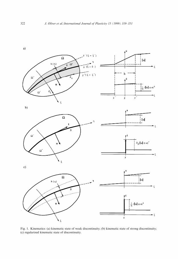
Fig. 1. Kinematics: (a) kinematic state of weak discontinuity; (b) kinematic state of strong discontinuity;

(c) regularized kinematic state of discontinuity.


where t stands for the time, and _�� stands for the time derivative of ��, �u�x; t� and��u��x; t� are continuous C0 displacement ®elds and Hh�x; t�, from now on namedthe unit ramp function, is also a continuous function in de®ned by:

Hh �0 x 2 ÿ

1 x 2 �� ÿ �ÿ�� ÿ �ÿ x 2 h

8><>: �2�

Clearly Hh exhibits a unit jump, as di�erence from its values at S� and Sÿ for thesame coordinate line � ��Hh �� Hh��; �� ÿHh��ÿ; �� 1 8��. From the de®ni-tion of Hh in Eq. (2) the corresponding gradient can be computed as:

rHh � 1

r�

@Hh

@�e� � 1

rn

@Hh

@�e� � �h

1

h�e�

h��; �� r��; �� ÿ �ÿ�h��0; �� r��0; �� ÿ �ÿ� � h��

�3�

where �h is a collocation function placed on h��h � 1 if x 2 h and �h � 0otherwise). From Eqs. (1) and (3) the kinematically compatible rate of strain _� canbe computed as:

where superscript ��s stands for the symmetric part of ��. Eq. (4) states that the rateof strain ®eld _� is the sum of a regular (continuous) part, _��x; t�, plus a dis-continuous part, �� _��x; t�, which exhibits jumps in Sÿ and S� [see Fig. 1(a)]. Eqs. (1)and (4) de®ne what will be referred to as kinematic state of weak discontinuity whichcan be qualitatively characterized by discontinuous, but bounded, (rate of) strain®elds.

2.2. Kinematic state of strong discontinuity

We can now de®ne the kinematic state of strong discontinuity as the limit caseof the one describing a weak discontinuity when the band h collapses to the dis-continuity line S [see Fig. 1(b)]. In other words, when S� and Sÿ simultaneouslytend to S [that is, with some abuse in the notation, �� ! 0, �ÿ ! 0, h�� ! 0, and,thus, h ! S in Fig. 1(a)]. In this case the unit ramp function (2) becomes a stepfunction HS�HS �x� � 0 8x 2 ÿ and HS�x� � 1 8x 2 �) and the rate of the dis-placement ®eld (1) reads:

_u�x; t� � _�u�x; t� �HS��_u��x; t� �5�

the corresponding compatible rate of strain being:


�6�

where �S is a line Dirac's delta-function placed in S. Now the (rate of) strain ®eld (6)can be decomposed into _��, exhibiting at most bounded discontinuities, and theunbounded counterpart �S��_u�� n�S . Thus, by contrast with the weak discontinuitycase, the strong discontinuity kinematic state can be characterized by the appearanceof unbounded (rate of) strain ®elds along the discontinuity line S.

2.3. Regularized kinematic state of discontinuity

Finally, we consider a kinematic state de®ned by the following rates of displace-ment and strain ®elds:

_u�x; t� � _�u�x; t� �HS��_u��x; t� �7�

where�S is a collocation function placed inS ��S�x� � 1 8x 2 S,�S�x� � 0 otherwise).Comparison of Eqs. (7) and (8) with Eqs. (1) to (6) suggests the following remarks:

Remark 2.1. The kinematic state de®ned by Eqs. (7) and (8) can be consideredrepresentative of a kinematic state of weak discontinuity of bandwidth h�� 6� 0 (seeFig. 1(c)) in the following sense:

. The velocity ®eld _u in Eq. (7) exhibits a jump of value ��_u�� across the dis-continuity line S, whereas in Eq. (1) the jump appears between both sides (Sÿand S�) of the discontinuity band h. If the bandwidth h�� is small with respectto the typical size of , the former is representative of the later.

. The _�� counterpart of the rate strain ®eld (8) di�ers from the corresponding onein Eq. (4) in that a step function HS is considered in the later instead of the unitramp function Hh in the former. On the other hand the term �� _�� in Eq. (8)coincides with the value of �� _�� in Eq. (4) evaluated at the points of S [note thath��0; �� h��, (see Eq. (3)) and that e��0; �� n��, (see Fig. 1(a)). In bothcases they are representative of the corresponding values in Eq. (4) if the band-width h�� is relatively small in comparison to the typical size of .

Remark 2.2 When the bandwidth h�� tends to zero the kinematic state de®ned by Eqs.(7) and (8) approaches a kinematic state of strong discontinuity as can be checked bycomparison with Eqs. (5) and (6) and realizing that when h�� ! 0, then�S=h�� ! �S .Remark 2.3. The rate of the strain ®eld (8) is not kinematically compatible with the dis-placement ®eld (7), in the sense that rs _u 6� _�, since rHS � �S n 6� ��S=h�� n.Compatibility is only approached when the bandwidth tends to zero as commented above.In the remainder of this paper we will consider Eqs. (7) and (8) as the description


of a kinematic state of weak discontinuity which approaches a kinematic state ofstrong discontinuity when the bandwidth h tends to zero.2 Observe that, now, akinematic state of weak discontinuity is characterized by a discontinuous (rate of)displacement ®eld (7), jumping across a material line S and an incompatible, anddiscontinuous across S, (rate of) strain ®eld (8) whose amplitude along S is char-acterized by the bandwidth h�� [see Fig. 1(c)].

3. The elastoplastic constitutive equations

In the rest of this work we will consider the classical elasto-plastic constitutiveequations which can be written as:

_� � C : � _�ÿ _�p�_�p � lm��_q � ÿlH�q��; q� � �� qÿ �y

m�� @��; q� � @�@�

�9�

where �, � and �p are the stress, total strain and plastic strain tensors, respectively,C is the elastic constitutive tensor (C � l1 1� �I, 1 and I being, respectively, therank-two and rank-four unit tensors and l and � the Lame's constants), q is thestress-like internal hardening variable, l is the plastic multiplier, � is the yield func-tion, �y is the yield stress, H is the hardening/softening parameter, and m� and mare, respectively, the plastic ¯ow tensor and the normal to the yield surface�q :� � ; ��; q� � 0f g (m � m� for associative plasticity). The model is supple-mented by the loading±unloading (Kuhn±Tucker) and consistency conditions:

�KuhnÿTucker� l50 ��; q�40 l��; q� � 0

�Consistency� l _��; q� � 0 if ��; q� � 0�10�

in such a way that the elastic and plastic behaviors are characterized by:

� < 0 ) l � 0 ) _� � C : _� �Elastic�

� � 0

_� < 0 ) l � 0 ) _� � C : _� �Elastic unloading�_� � 0 ) l � 0 � _q � 0� ) _� � C : _� �Neutral loading�

l > 0 � _q 6� 0� ) _� � Cep : _� �Plastic loading��8<: �11�

2 We could have started by de®ning a kinematic strain of weak discontinuity by means of Eqs. (7) and

(8) instead of Eqs. (1) and (4). However, the introduction made here can help to identify the compatible

kinematic state (7) and (8) as representative of the compatible, and consequently more familiar, kinematic

state de®ned in Section 2.1 and Fig. 1 (a).


where the tangent elasto-plastic constitutive tensor, Cep, and the plastic multiplier lcan be computed as:

Cep � Cÿ C : m� m : C

H�m� : C : m�12�

l � m : C : _�

H�m� : C : m�13�

4. The boundary value problem

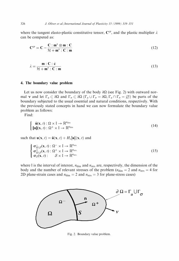
Let us now consider the boundary of the body @ (see Fig. 2) with outward nor-mal � and let ÿu � @ and ÿ� � @ �ÿu [ ÿ� � @;ÿu \ ÿ� �1� be parts of theboundary subjected to the usual essential and natural conditions, respectively. Withthe previously stated concepts in hand we can now formulate the boundary valueproblem as follows:

Find:

�u�x; t� : � I! Rndim

��u��x; t� : � � I! Rndim

��14�

such that u�x; t� � �u�x; t� �Hs��u��x; t� and�ÿnS�x; t� : ÿ � I! Rnstrs

��nS�x; t� : � � I! Rnstrs

�S�x; t� : S � I! Rnstrs

8<: �15�

where I is the interval of interest, ndim and nstrs are, respectively, the dimension of thebody and the number of relevant stresses of the problem (ndim � 2 and nstrs � 4 for2D plane-strain cases and ndim � 2 and nstrs � 3 for plane-stress cases)

Fig. 2. Boundary value problem.


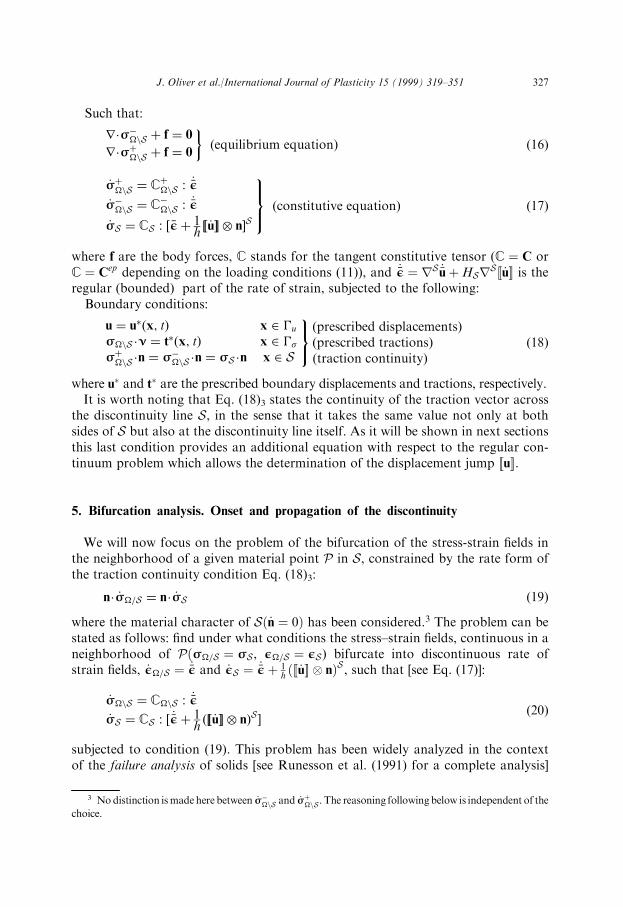
Such that:

r��ÿnS � f � 0

r��nS � f � 0

��equilibrium equation� �16�

_��nS � C�nS : _��

_�ÿnS � CÿnS : _��

_�S � CS : � �� 1h��_u�� n�S

9>=>; �constitutive equation� �17�

where f are the body forces, C stands for the tangent constitutive tensor (C � C orC � Cep depending on the loading conditions (11)), and _�� rS _�u�HSrS��_u�� is theregular (bounded) part of the rate of strain, subjected to the following:

Boundary conditions:

u � u��x; t� x 2 ÿu

�nS �� t��x; t� x 2 ÿ��nS �n � �ÿnS �n � �S �n x 2 S

9=; �prescribed displacements��prescribed tractions��traction continuity�

�18�

where u� and t� are the prescribed boundary displacements and tractions, respectively.It is worth noting that Eq. (18)3 states the continuity of the traction vector across

the discontinuity line S, in the sense that it takes the same value not only at bothsides of S but also at the discontinuity line itself. As it will be shown in next sectionsthis last condition provides an additional equation with respect to the regular con-tinuum problem which allows the determination of the displacement jump ��u��.

5. Bifurcation analysis. Onset and propagation of the discontinuity

We will now focus on the problem of the bifurcation of the stress-strain ®elds inthe neighborhood of a given material point P in S, constrained by the rate form ofthe traction continuity condition Eq. (18)3:

n� _�=S � n� _�S �19�where the material character of S�_n � 0� has been considered.3 The problem can bestated as follows: ®nd under what conditions the stress±strain ®elds, continuous in aneighborhood of P��=S � �S, �=S � �S) bifurcate into discontinuous rate ofstrain ®elds, _�=S � _�� and _�S � _�� 1

h ��_u�� n�S , such that [see Eq. (17)]:

_�nS � CnS : _��

_�S � CS : � _�� 1h��_u�� n�S� �20�

subjected to condition (19). This problem has been widely analyzed in the contextof the failure analysis of solids [see Runesson et al. (1991) for a complete analysis]

3 No distinction ismadehere between _�ÿnS and _��nS . The reasoning following below is independent of the

choice.


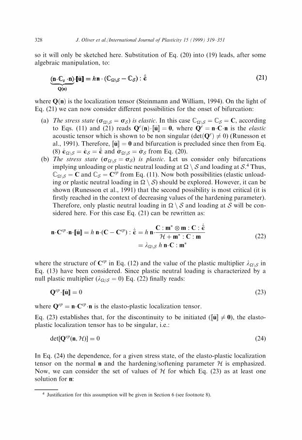
so it will only be sketched here. Substitution of Eq. (20) into (19) leads, after somealgebraic manipulation, to:

where Q�n� is the localization tensor (Steinmann and William, 1994). On the light ofEq. (21) we can now consider di�erent possibilities for the onset of bifurcation:

(a) The stress state (�nS � �S) is elastic. In this case CnS � CS � C, accordingto Eqs. (11) and (21) reads Qe�n��_u�� 0, where Qe � n�C�n is the elasticacoustic tensor which is shown to be non singular (det�Qe� 6� 0) (Runesson etal., 1991). Therefore, ��_u�� 0 and bifurcation is precluded since then from Eq.(8) _�nS � _�S � _�� and _�nS � _�S from Eq. (20).

(b) The stress state (�nS � �S) is plastic. Let us consider only bifurcationsimplying unloading or plastic neutral loading at n S and loading at S.4 Thus,CnS � C and CS � Cep from Eq. (11). Now both possibilities (elastic unload-ing or plastic neutral loading in n S) should be explored. However, it can beshown (Runesson et al., 1991) that the second possibility is most critical (it is®rstly reached in the context of decreasing values of the hardening parameter).Therefore, only plastic neutral loading in n S and loading at S will be con-sidered here. For this case Eq. (21) can be rewritten as:

n�Cep �n��_u�� h n��Cÿ Cep� : _�� h n�C : m� m : C : _��

H�m� : C : m

� lnS h n�C : m��22�

where the structure of Cep in Eq. (12) and the value of the plastic multiplier lnS inEq. (13) have been considered. Since plastic neutral loading is characterized by anull plastic multiplier (l=S � 0) Eq. (22) ®nally reads:

Qep ��_u�� 0 �23�

where Qep � n�Cep �n is the elasto-plastic localization tensor.

Eq. (23) establishes that, for the discontinuity to be initiated (��_u�� 6� 0), the elasto-plastic localization tensor has to be singular, i.e.:

det�Qep�n;H�� 0 �24�

In Eq. (24) the dependence, for a given stress state, of the elasto-plastic localizationtensor on the normal n and the hardening/softening parameter H is emphasized.Now, we can consider the set of values of H for which Eq. (23) as at least onesolution for n:

4 Justi®cation for this assumption will be given in Section 6 (see footnote 8).


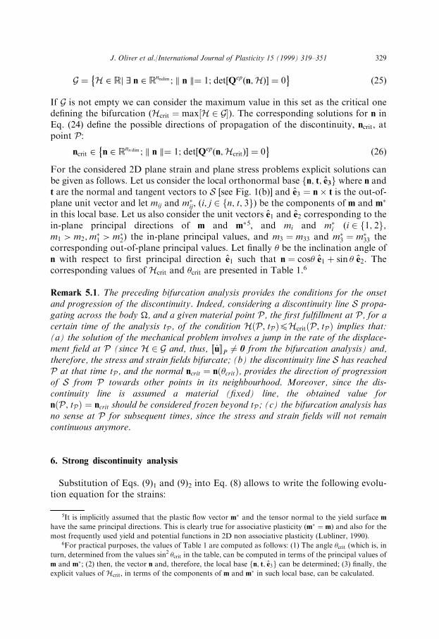
G � H 2 Rj 9 n 2 Rnndim ; k n k� 1; det�Qep�n;H�� 0� �25�

If G is not empty we can consider the maximum value in this set as the critical onede®ning the bifurcation (Hcrit � max�H 2 G�). The corresponding solutions for n inEq. (24) de®ne the possible directions of propagation of the discontinuity, ncrit, atpoint P:

ncrit 2 n 2 Rnn dim ; k n k� 1; det�Qep�n;Hcrit�� 0� �26�

For the considered 2D plane strain and plane stress problems explicit solutions canbe given as follows. Let us consider the local orthonormal base n; t; e3f g where n andt are the normal and tangent vectors to S [see Fig. 1(b)] and e3 � n� t is the out-of-plane unit vector and let mij and m�ij, (i; j 2 n; t; 3f g) be the components of m and m�

in this local base. Let us also consider the unit vectors e1 and e2 corresponding to thein-plane principal directions of m and m�5, and mi and m�i (i 2 1; 2f g;m1 > m2;m

�1 > m�2) the in-plane principal values, and m3 � m33 and m�3 � m�33 the

corresponding out-of-plane principal values. Let ®nally � be the inclination angle ofn with respect to ®rst principal direction e1 such that n � cos� e1 � sin � e2. Thecorresponding values of Hcrit and �crit are presented in Table 1.6

Remark 5.1. The preceding bifurcation analysis provides the conditions for the onsetand progression of the discontinuity. Indeed, considering a discontinuity line S propa-gating across the body , and a given material point P, the ®rst ful®llment at P, for acertain time of the analysis tP , of the condition H�P; tP�4Hcrit�P; tP� implies that:(a) the solution of the mechanical problem involves a jump in the rate of the displace-ment ®eld at P (since H 2 G and, thus, ��_u��P 6� 0 from the bifurcation analysis) and,therefore, the stress and strain ®elds bifurcate; (b) the discontinuity line S has reachedP at that time tP , and the normal ncrit � n��crit�, provides the direction of progressionof S from P towards other points in its neighbourhood. Moreover, since the dis-continuity line is assumed a material (®xed) line, the obtained value forn�P; tP� � ncrit should be considered frozen beyond tP; (c) the bifurcation analysis hasno sense at P for subsequent times, since the stress and strain ®elds will not remaincontinuous anymore.

6. Strong discontinuity analysis

Substitution of Eqs. (9)1 and (9)2 into Eq. (8) allows to write the following evolu-tion equation for the strains:

5It is implicitly assumed that the plastic ¯ow vector m� and the tensor normal to the yield surface m

have the same principal directions. This is clearly true for associative plasticity (m� � m) and also for the

most frequently used yield and potential functions in 2D non associative plasticity (Lubliner, 1990).6For practical purposes, the values of Table 1 are computed as follows: (1) The angle �crit (which is, in

turn, determined from the values sin2 �crit in the table, can be computed in terms of the principal values of

m and m�; (2) then, the vector n and, therefore, the local base n; t; e3f g can be determined; (3) ®nally, the

explicit values of Hcrit, in terms of the components of m and m� in such local base, can be calculated.


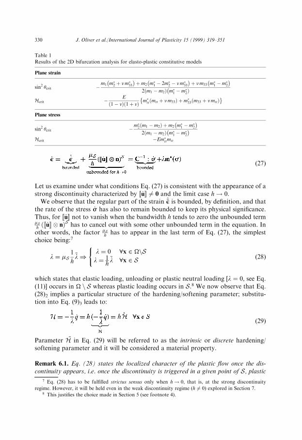
�27�

Let us examine under what conditions Eq. (27) is consistent with the appearance of astrong discontinuity characterized by ��_u�� 6� 0 and the limit case h! 0.We observe that the regular part of the strain _�� is bounded, by de®nition, and that

the rate of the stress _� has also to remain bounded to keep its physical signi®cance.Thus, for ��_u�� not to vanish when the bandwidth h tends to zero the unbounded term�Sh ��_u�� n�S has to cancel out with some other unbounded term in the equation. Inother words, the factor �S

h has to appear in the last term of Eq. (27), the simplestchoice being:7

l � �S 1h

�l) l � 0 8x 2 nSl � 1

h�l 8x 2 S

(�28�

which states that elastic loading, unloading or plastic neutral loading [l � 0, see Eq.(11)] occurs in n S whereas plastic loading occurs in S.8 We now observe that Eq.(28)2 implies a particular structure of the hardening/softening parameter; substitu-tion into Eq. (9)3 leads to:

�29�

Parameter �H in Eq. (29) will be referred to as the intrinsic or discrete hardening/softening parameter and it will be considered a material property.

Remark 6.1. Eq. (28) states the localized character of the plastic ¯ow once the dis-continuity appears, i.e. once the discontinuity is triggered in a given point of S, plastic

Table 1

Results of the 2D bifurcation analysis for elasto-plastic constitutive models

Plane strain

sin2 �crit ÿm1 m�2 � �m�33ÿ ��m2 m�1 ÿ 2m�2 ÿ �m�33

ÿ �� m33 m�1 ÿm�2ÿ �

2 m1 ÿm2� � m�1 ÿm�2�ÿ

Hcrit ÿ E

1ÿ �� 1� �� m�tt mtt � �m33� � �m�33 m33 � �mtt� �� Plane stress

sin2 �crit ÿm�2 m1 ÿm2� � �m2 m�1 ÿm�2ÿ �

2 m1 ÿm2� � m�1 ÿm�2ÿ �

Hcrit ÿEm�ttmtt

7 Eq. (28) has to be ful®lled strictus sensus only when h! 0, that is, at the strong discontinuity

regime. However, it will be held even in the weak discontinuity regime (h 6� 0) explored in Section 7.8 This justi®es the choice made in Section 5 (see footnote 4).


strain rate is only allowed to develop at this point whereas its neighborhood at n Sexperiences elastic loading or unloading (l �0).

Remark 6.2. Eq. (29) shows that as long as the strong discontinuity regime is approached(h!0) the hardening/softening parameterH tends to zero. Thus the strong discontinuityregime is only consistent with the part of the hardening/softening branch with null slope.

We can now rewrite Eq. (27) restricted to points of S and considering Eqs. (28) and(29), as:

�30�

and we realize that as the strong discontinuity regime is approached (h! 0) theunbounded terms have to cancel out each other leading to:

��_n�� n� �S� ÿ 1

�H _q m� �S� � �31�

6.1. Strong discontinuity condition

Eq. (31), that will be referred to as the strong discontinuity equation, establishes theevolution of the jump in the strong discontinuity regime and can be now specializedfor the considered 2D problems.

6.1.1. Plane strainLet us now focus on the 2D plane-strain problem considering, at any point of S,

the orthonormal base n; t; e3f g de®ned in Section 5. In this base the (rate of) thedisplacement jump can be written as ��_u�� _un��n� �� _ut��t, where ��un�� and ��ut�� are thenormal and tangential components of the displacement jump at S, and Eq. (31)reads, in terms of components:

�� _un�� 12�� _ut�� 0

12�� _ut�� 0 00 0 0

264375 � ÿ 1

�H _qm�nn m�nt 0m�nt m�tt 00 0 m�33

24 35s

�32�

where m�ab; a; b 2 n; t; 3f g are the components of the plastic ¯ow tensor m� in thechosen base. Eq. (32) can be regarded as a system of four non trivial equations withtwo unknowns (�� _un��; �� _ut��) so that two equations involving only the ¯ow tensorcomponents m�ij can be extracted. They clearly are:

m�ttS � 0 ; m�33S � 0 �33�

6.1.2. Plane stressPlane stress cases have to be studied in the projected space obtained by elimina-

tion of the out-of-plane components of the stresses and the strains. In this case Eq.(31) reads, in terms of components:


�� _un�� 12�� _ut��

12�� _ut�� 0

" #� ÿ 1

�H _qm�nn m�ntm�nt m�tt

� �s

�34�

Here the system Eq. (34) includes three equations with the two unknowns �� _un�� and�� _ut�� so that the following condition emerges:

m�ttS � 0 �35�Eq. (33) and Eq. (35), which will be named strong discontinuity conditions, are

clearly necessary conditions for the formation of a strong discontinuity. They arenot, in general, ful®lled at the initial stages of the plastic ¯ow and preclude, in mostof cases, the formation of an strong discontinuity just at the bifurcation stage.

Remark 6.3. It is illustrating to realize that substitution of conditions Eqs. (33) and(35) into the values of Hcrit in Table 1 gives, both in the plane strain and plane stresscases, Hcrit � 0. This result can be justi®ed as follows: (a) Eq. (21) holds at any stageof the problem since it comes from Eqs. (19) and (20) which hold for all the stages ofthe analysis; (b) the strong discontinuity regime is characterized by the limit caseh! 0 which implies that, for ��_u�� 6�0 in Eq. (21) and loading cases (CS � C

epS , then

det n�CepS �n

ÿ �� det Q n;H� �� 0; (c) according to Eq. (29) at the strong dis-continuity regime h! 0) H � 0, whereby det Q n;H� �� jH=0=0; (d) therefore,H �0 belongs to the set G [see Eq. (25)] of solutions for H of Eq. (24), which is givenby the values H4Hcrit. In other words: the solution ��_u�� of the strong discontinuityproblem lies in the null space of the perfectly plastic (H �0) localization tensor.9

Remark 6.4. In particular Hcrit �0 is a necessary condition to induce a strong dis-continuity. If that condition occurs at the bifurcation stage the bifurcation could takeplace under the form of a strong discontinuity. In the general case (Hcrit 6�0) bifurcationwill take place under the form of a weak discontinuity and the strong discontinuity con-ditions (33) or (35) must be induced in subsequent stages. In Section 7 a procedure tomodel the transition from the weak to the strong discontinuity regimes is proposed.

Remark 6.5. Bifurcation analysis of plastic models shows that, for the associative case(m � m�) it occurs that Hcrit �� 40. Moreover, for most of the stress states it isstrictly Hcrit <0 and, according to previous remarks, bifurcation can not take place inthe form of a strong discontinuity. On the contrary, for non associative plasticity(m 6� m�) it often happens that Hcrit �� >0, which could suggest that, since H � 0belongsto the set of admissible values G in Eq. (25), such value of the stresses is com-patible with a bifurcation in the strong discontinuity fashion. However, the necessarystrong discontinuity conditions Eqs. (33) or (35) and the subsequent necessary condi-tion Hcrit �� 0 clearly preclude such possibility. Actually, this only refers to the bifur-cation in a strong discontinuity fashion and not to the possibility of bifurcating under aweak discontinuity form and developing a strong discontinuity in subsequent stages.

9 This result was ®rstly stated in Simo et al. (1993).


6.2. Discrete constitutive equation

From Eqs. (9)4 and (9)5 and the consistency condition for loading cases( _� � m : _�� _q � 0) the strong discontinuity Eq. (31) can be written:

��_u�� n�S � 1

�H m �S� � : _� �S� �� m� �s� � �36�

which is regarded in conjunction with the traction continuity Eq. (18)3

tnS � �nS �n � �S �n �37�

Eqs. (36) and (37) constitute, for any point of S, a system of nine non trivial alge-braic equations which states, for the general 3D case, the implicit dependence ofnine unknowns (the six stress components �S and the three jump components ��u��)on the traction vector tnS:

�S � F tnS t� �� 38��u�� I tnS t� �� 39�

Remark 6.6. Eq. (39) de®nes a discrete (traction- vs jump) constitutive equation at theinterface S. It is worth noting that it emerges naturally (consistently) from the con-tinuum (stress-vs-strain) elasto-plastic constitutive equation described in Section 3 whenthe strong discontinuity kinematics is enforced. Thus, it is not strictly necessary neitherto derive nor to make e�ective use of such discrete constitutive equation for modeling andnumerical simulation purposes. In fact, the numerical solution scheme shown in Section 9does not include the derivation of such equation and deals only with the standard elasto-plastic constitutive equation of Section 3 as the source constitutive equation.

6.2.1. Example I: J2 (Von Mises) associative plasticity in plane strainThis case is characterized by the following expressions for the yield surface and the

plastic ¯ow tensor:

� �; q� � � �� qÿ �y �� 32

qk S k

� �m � m� � @�@� �

��32

qSk S k

�40�

where S and �� stand for the deviatoric stresses and the e�ective stress, respectively.Specialization of Eqs. (32) and (36) for this case leads to:

�� _un�� 12�� _ut�� 0

12�� _ut�� 0 00 0 0

264375 � 1

�H3

2

S : _S

S : S

!S

Snn Snt 0Snt Stt 00 0 S33

24 35S

�41�

From Eq. (41) it is immediately obtained that S33S � SttS � 0 and then, due to thedeviatoric character of S Tr Sf g � Snn � Stt � S33 � 0� ), also SnnS � 0. Therefore the


only non zero component of S is Snt �S � Snt n t� � � Snt t n� �� and thenS : _Sÿ �

= S : S� � � _Snt=Snt so that ®nally we obtain from Eq. (41) the additional rela-tionships �� _un�� 0 and �� _ut�� 3= �Hÿ �

_SntS . Hence, Eq. (41) is equivalent to the fol-lowing system:

�nnS � � � SnnS � � �ntS � SntS � ��ttS � � � SttS � � �33S � � � S33S � �

��42�

�� _un�� 0

�� _ut�� 3�H _�

(�43�

where � (the mean stress) ant � remain as unknowns. They can be determined byresorting to the two equations provided by the traction continuity condition Eq. (37)which for this 2D case read: �nnS � �nnnS � � and �ntS � �ntnS � �.

6.2.2. Example II: 2D Rankine associative plasticity.The yield surface and ¯ow tensor are now:

� �; q� � � �1 �� qÿ �ym � m� � p1 p1

�44�

where �1 stands for the maximum in-plane principal stress (�1 > �2) and p1 is theassociated unit vector in the corresponding principal direction which is inclined theangle � with respect to n p1 � cos� n� sin � t� �. In the base n; t; e3gf Eq. (36) nowreads:

�� _un�� 12�� _ut�� 0

12�� _ut�� 0 00 0 0

264375 � 1

�H _�1� �Scos2� sin � cos� 0

sin � cos� sin2 � 00 0 0

24 35 �45�

where the result m : _� � _�1 has been considered. From the component (.)22 of Eq.(45) we obtain sin2 � � 0 so that � � 0 and n � p1. Thus, n is the ®rst principaldirection, then �ntS � 0 and the discontinuity line S develops perpendicularly to the®rst principal stress. Since sin � � 0 from component ��12 of that equation we obtain�� _ut�� 0 and, ®nally, �� _un�� _�1� �S

�H from component ��11.Therefore, Eq. (45) can be equivalently rewritten as:

�nnS � �1S � ��ntS � 0

��46�

�� _un�� 1�H _�

�� _ut�� 0

(�47�


where �, the ®rst principal stress, remains as an unknown that can be determinedthrough the traction continuity condition �nnS � �nnnS � �.

Remark 6.7. Eqs. (43) and (47) with � � �nnnS and � � �ntnS are specializations ofthe general form Eq. (39) for the considered J2 (plane strain) and Rankine plasticityproblems. Observe that the discrete constitutive Eq. (43) states that only the tangentcomponent of the jump ��ut�� can develop (��un�� 0) so that with this type of J2 plasticityequations the generated strong discontinuity is a slip line (this result was also found inSimo et al., 1993; Oliver, 1996a; Armero and Garikipati, 1996).On the contrary Eq.(47) states that with Rankine-type plasticity models only Mode I (in terms of FractureMechanics) strong discontinuities can be modeled since the tangent component of thejump ��ut�� 0. Obtaining such explicit forms of the discrete constitutive equations is notso straight-forward for other families of elastoplastic models. This makes speciallyrelevant a methodology to approach strong discontinuities that does not require theexplicit statement of such equations as pointed out in Remark 6.6.

7. A variable bandwidth model

The bifurcation and strong discontinuity analyzes performed in Sections 6 and 7above provide signi®cant information about the mechanism to induce strong dis-continuities. This can be summarized as follows:

. Bifurcation of the stress-strain ®elds is a necessary condition for the inceptionof a discontinuity in the displacement ®eld. In the context of a variable hard-ening (or softening) law that bifurcation will take place, for a given materialpoint, when the condition H �� 4Hcrit �� is ful®lled for the ®rst time. In gen-eral Hcrit �� will be non zero (Remark 6.5).

. Bifurcation will not, in general, produce the strong discontinuity. The neces-sary condition (to induce a strong discontinuity) Hcrit �� 0 will not, in gen-eral, be ful®lled at the bifurcation stage (Remarks 6.4 and 6.5) and bifurcationwill take place under the form of a weak discontinuity.

. If the hardening/softening parameter H is expressed in terms of the intrinsichardening/softening parameter �H (considered a material property) and thebandwidth h, according to Eq. (29) (i.e. H � h �H) then the bandwidth char-acterizing the weak discontinuity at the bifurcation will be given byhcrit � Hcrit= �Hÿ � 6� 0.

Therefore, if the aim of the model is to capture strong discontinuities an addi-tional ingredient has to be introduced which provides: (a) the transition of thebandwidth from the value hcrit 6� 0, at the bifurcation, to the value h � 0, in a sub-sequent time and (b) the ful®llment of the strong discontinuity conditions Eqs. (33)or (35). In Fig. 3 what has been termed variable bandwidth model (Oliver et al., 19971998; Oliver, 1998) is sketched. It can be described in the following steps:


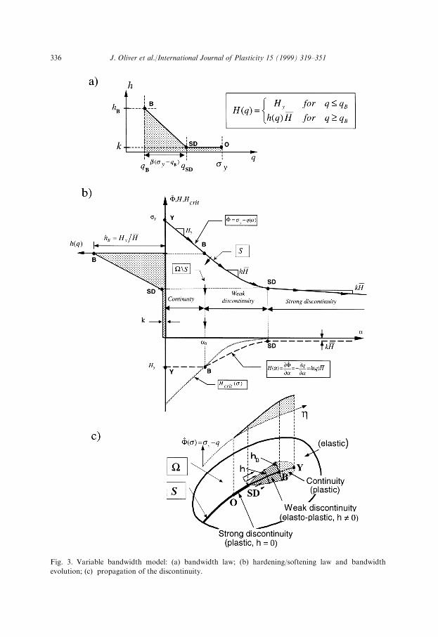
Fig. 3. Variable bandwidth model: (a) bandwidth law; (b) hardening/softening law and bandwidth

evolution; (c) propagation of the discontinuity.


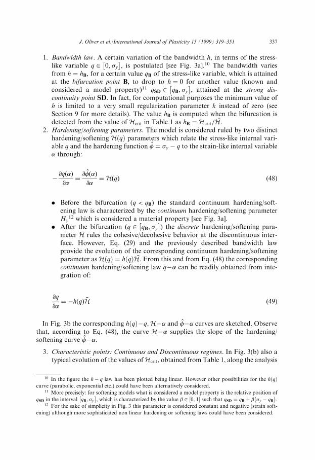
1. Bandwidth law. A certain variation of the bandwidth h, in terms of the stress-like variable q 2 0; �y

� �, is postulated [see Fig. 3a].10 The bandwidth varies

from h � hB, for a certain value qB of the stress-like variable, which is attainedat the bifurcation point B, to drop to h � 0 for another value (known andconsidered a model property)11 qSD 2 qB; �y

� �, attained at the strong dis-

continuity point SD. In fact, for computational purposes the minimum value ofh is limited to a very small regularization parameter k instead of zero (seeSection 9 for more details). The value hB is computed when the bifurcation isdetected from the value of Hcrit in Table 1 as hB � Hcrit= �H.

2. Hardening/softening parameters. The model is considered ruled by two distincthardening/softening H q� � parameters which relate the stress-like internal vari-able q and the hardening function � � �y ÿ q to the strain-like internal variable� through:

ÿ @q �� @�� @� ��

@�� H q� � �48�

. Before the bifurcation (q < qB) the standard continuum hardening/soft-ening law is characterized by the continuum hardening/softening parameterHy

12 which is considered a material property [see Fig. 3a].. After the bifurcation (q 2 qB; �y

� �) the discrete hardening/softening para-

meter �H rules the cohesive/decohesive behavior at the discontinuous inter-face. However, Eq. (29) and the previously described bandwidth lawprovide the evolution of the corresponding continuum hardening/softeningparameter as H q� � � h q� � �H. From this and from Eq. (48) the correspondingcontinuum hardening/softening law qÿ� can be readily obtained from inte-gration of:

@q

@�� ÿh q� � �H �49�

In Fig. 3b the corresponding h q� �ÿq;Hÿ� and �ÿ� curves are sketched. Observethat, according to Eq. (48), the curve Hÿ� supplies the slope of the hardening/softening curve �ÿ�.

3. Characteristic points: Continuous and Discontinuous regimes. In Fig. 3(b) also atypical evolution of the values ofHcrit, obtained from Table 1, along the analysis

10 In the ®gure the hÿ q law has been plotted being linear. However other possibilities for the h q� �curve (parabolic, exponential etc.) could have been alternatively considered.

11 More precisely: for softening models what is considered a model property is the relative position of

qSD in the interval qB; �y� �

, which is characterized by the value � 2 0; 1� � such that qSD � qB � � �y ÿ qBÿ �

.12 For the sake of simplicity in Fig. 3 this parameter is considered constant and negative (strain soft-

ening) although more sophisticated non linear hardening or softening laws could have been considered.


is plotted. For a given material point yielding begins at point Y of Fig. 3(b), inwhich the hardening/softening parameter takes the value Hy. While Hcrit < Hy

bifurcation is precluded and the behavior is continuous. As soon as Hcrit � Hy

the bifurcation point B is detected: the corresponding values of n �crit� � arecomputed from Table 1 which, once introduced in the rest of the model, war-rant that bifurcation at point B takes place under the appropriate loading (atS) and unloading (at n S) conditions [see Fig. 3(b)]. Also at this point thevalue hB � Hcrit= �H, which states the initial value of the bandwidth law ofFig. 3(a), is computed. Since in general hB 6� 0, point B corresponds to theonset of a weak discontinuity whose bandwidth is enforced to decrease by thebandwidth law of Fig. 3(a) beyond this point. As soon as the value q � qSD isattained at point SD and, according to the bandwidth law, h � k � 0 thestrong discontinuity regime is reached and the strong discontinuity conditionsEq. (33) or (35) are naturally induced. Finally, beyond point SD the strongdiscontinuity regime develops keeping the bandwidth h and the continuumhardening/softening parameter H in a null (k-regularized) value.

Remark 7. Since consistency with the results obtained from the bifurcation and strongdiscontinuity analyzes is kept along the process the obtained results warrant that: (a)bifurcation takes place under the appropriate loading±unloading conditions, thus notleading to a two materials approach (Oliver et al., 1997); and (b) the rate of thestresses remain bounded along the whole process keeping their physical signi®cance.

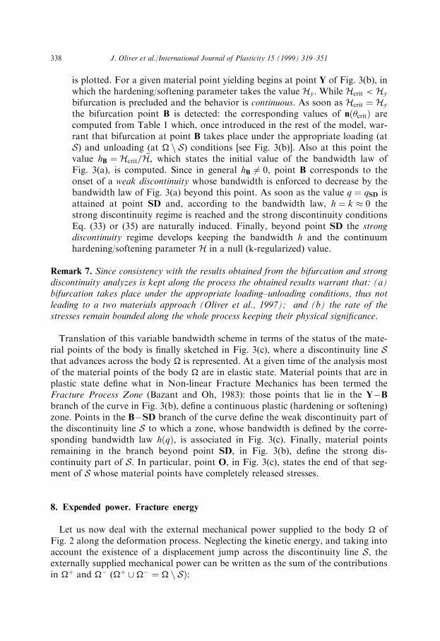
Translation of this variable bandwidth scheme in terms of the status of the mate-rial points of the body is ®nally sketched in Fig. 3(c), where a discontinuity line Sthat advances across the body is represented. At a given time of the analysis mostof the material points of the body are in elastic state. Material points that are inplastic state de®ne what in Non-linear Fracture Mechanics has been termed theFracture Process Zone (Bazant and Oh, 1983): those points that lie in the YÿBbranch of the curve in Fig. 3(b), de®ne a continuous plastic (hardening or softening)zone. Points in the BÿSD branch of the curve de®ne the weak discontinuity part ofthe discontinuity line S to which a zone, whose bandwidth is de®ned by the corre-sponding bandwidth law h q� �, is associated in Fig. 3(c). Finally, material pointsremaining in the branch beyond point SD, in Fig. 3(b), de®ne the strong dis-continuity part of S. In particular, point O, in Fig. 3(c), states the end of that seg-ment of S whose material points have completely released stresses.

8. Expended power. Fracture energy

Let us now deal with the external mechanical power supplied to the body ofFig. 2 along the deformation process. Neglecting the kinetic energy, and taking intoaccount the existence of a displacement jump across the discontinuity line S, theexternally supplied mechanical power can be written as the sum of the contributionsin � and ÿ (� [ÿ � n S�:


where the traction vector continuity condition n��nS � n��ÿnS � n��S� �

has beenconsidered. We observe in Eq. (50) that Pint

nS and PintS are volumetric and surface

counterparts of the supplied external power, respectively. Thus, we can understandPintS as the part of the external power internally spent in the formation of the jump��_u�� at the discontinuity interface S. Therefore, taking into account Eq. (30) we canwrite Pint

S , after some algebraic manipulation, as:

�51�

We now observe that the ®rst integral of the right-hand-side of Eq. (51) is boundedand tends to zero with the bandwidth h. Thus, if the bandwidth is small with respectto the representative size of it can be neglected. Let us now specialize the problemto the cases ful®lling the following conditions:

1. The function � �� in Eq. (9)4 is an homogeneous function (of degree one) ofthe stresses.13 In this case, in virtue of Euler's theorem for homogeneous func-tions, it can be written:

@�� : � � � �� 52�

2. Associative plasticity (m� � m � @��)3. Strain-softening (which implies that q remains in the bounded interval 0; �y

� �)

We also observe that, for loading processes (l 6� 0), Eq. (10)1 implies that � � 0,and, thus, �y ÿ q � � � @� � : � � m : � [see Eqs. (9)4, (9)5 and (52)]. So that,®nally, Eq. (51) can be written as:

13 This is a requirement ful®lled by many usual yield functions [Von-Mises, Tresca, Mohr±Coulomb,

Drucker Prager, Rankine, etc. (Khan, 1995).


�53�

Let us now compute the energy WS spent at S along any loading process leading tothe formation of a strong discontinuity. The complete loading process can be char-acterized by the evolution of the stress-like variable q ranging from q � 0 at theunloaded initial state (t � 0) to q � �y at the ®nal state (t � t1) where the stressesare compleately released:

The kernel of the last integral of Eq. (54) can be now identi®ed as the energy spent,per unit of surface, in the formation of the strong discontinuity which, in the contextof the non-linear fracture mechanics, is referred to as the fracture energy Gf. In viewof Eqs. (53) and (54) it can be written:

Gf ��t10

@

@t' q� �dt �

�q��yq�0

@

@q' q� �dq � ' �y

ÿ �ÿ ' 0� � � ÿ 1

2

�2y�H �55�

so that, ®nally, Eq. (55) can be solved for the intrinsic hardening/softening para-meter, �H, in terms of the material properties �y and Gf as:

�H � ÿ 1

2

�2yGf

�56�

Remark 8.1. Results (55) and (56) have been obtained for an arbitrary loading pro-cess. The material property character of the resulting fracture energy, lies cruciallyonto this fact since the value of Gf in Eq. (55) is independent of the loading process.This result, in turn, comes out directly from Eq. (53), namely: �S: ��_u�� n�s is anexact time di�erential (�S : ��_u�� n� �s� @

@t ' q� ��. Notice that this is not a completelygeneral result since it has been obtained under the conditions (a)±(c) above.

Remark 8.2. The existence of the fracture energy as a bounded and positive materialproperty is then restricted to associative plasticity models with strain softeningaccording to conditions (b) and (c). In fact, there is no intrinsic restriction for non-associative strain-hardening constitutive equations to induce strong discontinuities. Inthat case the intrinsic hardening/softening parameter �H would have to be positive


according to the condition �H � H=h� � > 0. However, this scenario does not ensure nei-ther the existence of the fracture energy, as a material property independent of theloading process, nor a bounded value for the energyWS in Eq. (54) (since in that caseq 2 �0;ÿ1�). On the other hand, the positiveness of �H would lead to a cohesive (insteadof decohesive) character of the resulting discrete constitutive equation at the interface.

9. Finite element simulation. Computational aspects

The ingredients of the approach presented above can now be considered for thenumerical simulation of strong discontinuities, via ®nite elements. It was pointed outin Remark 6.6 that the discrete (stress-jump) constitutive Eq. (39) obtained from thestrong discontinuity analysis is not in fact used for numerical simulation purposesbut, on the contrary, it emerges naturally from the continuum stress-straincon-stitutive equation when the strong discontinuity kinematics is enforced. In con-sequence, a standard ®nite element code for 2D elasto-plastic analysis only needssome few modi®cations to implement the present model. Essentially these are:

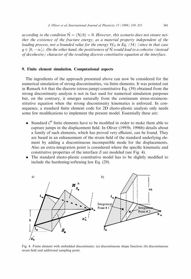
. Standard C0 ®nite elements have to be modi®ed in order to make them able tocapture jumps in the displacement ®eld. In Oliver (1995b, 1996b) details abouta family of such elements, which has proved very e�cient, can be found. Theyare based in an enhancement of the strain ®eld of the standard underlying ele-ment by adding a discontinuous incompatible mode for the displacements.Also an extra-integration point is considered where the speci®c kinematic andconstitutive properties of the interface S are modeled (see Fig. 4).

. The standard elasto-plastic constitutive model has to be slightly modi®ed toinclude the hardening/softening law Eq. (29).

Fig. 4. Finite element with embedded discontinuity: (a) discontinuous shape function; (b) discontinuous

strain ®eld and additional sampling point.


. Computation of the bifurcation condition H < Hcrit and the correspondingdirection of propagation of the discontinuity has to be included. For 2D casesresults in Table 1 can be used. Also the bifurcation bandwidth of Eq. (48) andthe bandwidth evolution of Eq. (49) have to be computed according to thevalues Hcrit in Table 1.

. In a strain driven algorithm, Eq. (8) has to be numerically integrated to obtainthe strain ®eld at any given time of the analysis. In fact the rate of the strain®eld at S:

_"S � _�"� 1

h q� � ��_u�� n� �S �57�

cannot be analytically integrated due to the appearance of h q �"; ��u�� which is givenin Eq. (49). In the examples shown below the following mid-point rule (second orderaccuracy) has been used:

where subscripts ��t��t and ��t refer to evaluation at the end of two consecutive timesteps and � �� t��tÿ ��t are the corresponding increments.

. In order to avoid ill-conditioning in Eq. (57) when h! 0, the evolution of hgiven by Eq. (49) is limited to h 2 hcrit; k� � where k > 0 is a very small regular-ization parameter. Typically, k is taken about 10ÿ2±10ÿ3 times the size of the®nite element. In Oliver (1995a, 1996b) the objectivity (independence) of theresults with respect to such regularization parameter is shown, provided it issmall with respect to the typical ®nite element size.

10. A ®rst illustrative example: uniaxial tension test

A very simple, but illustrative, example is now examined in order to assess thecapacity of the approach to induce strong discontinuities and to reproduce the the-oretical predictions of the strong discontinuity analysis (essentially, the discreteconstitutive equation at the interface). A J2 (Von-Mises) model of associative plas-ticity is taken as target constitutive equation and the results are checked via an uni-axial tension test under plane strain conditions. In Fig. 5(a) the loading andgeometrical features of the problem are presented. A linear bandwith law with� � 0:15 has been taken. Since the stress ®eld is uniform, the discontinuity must beseeded somewhere; therefore, the lower left corner element of the unstructured ®nite


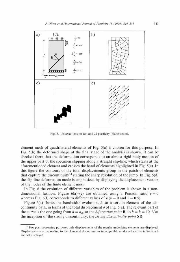
element mesh of quadrilateral elements of Fig. 5(a) is chosen for this purpose. InFig. 5(b) the deformed shape at the ®nal stage of the analysis is shown. It can bechecked there that the deformation corresponds to an almost rigid body motion ofthe upper part of the specimen slipping along a straight slip-line, which starts at theaforementioned element and crosses the band of elements highlighted in Fig. 5(c). Inthis ®gure the contours of the total displacements group in the patch of elementsthat capture the discontinuity14 stating the sharp resolution of the jump. In Fig. 5(d)the slip-line deformation mode is emphasized by displaying the displacement vectorsof the nodes of the ®nite element mesh.In Fig. 6 the evolution of di�erent variables of the problem is shown in a non-

dimensional fashion. Figure 6(a)±(e) are obtained using a Poisson ratio � � 0whereas Fig. 6(f) corresponds to di�erent values of � (� � 0 and � � 0:5).Figure 6(a) shows the bandwidth evolution, h, at a certain element of the dis-

continuity path, in terms of the total displacement � of Fig. 5(a). The relevant part ofthe curve is the one going from h � hB, at the bifurcation point B, to h � k � 10ÿ3l atthe inception of the strong discontinuity, the strong discontinuity point SD.

Fig. 5. Uniaxial tension test and J2 plasticity (plane strain).

14 For post-processing purposes only displacements of the regular underlying elements are displayed.

Displacements corresponding to the elemental discontinuous incompatible modes referred to in Section 9

are not displayed.


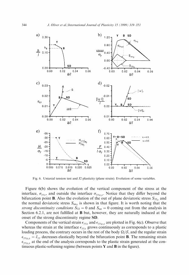
Figure 6(b) shows the evolution of the vertical component of the stress at theinterface, �yyS , and outside the interface �yynS . Notice that they di�er beyond thebifurcation point B. Also the evolution of the out of plane deviatoric stress S33S andthe normal deviatoric stress SnnS is shown in that ®gure. It is worth noting that thestrong discontinuity conditions S33 � 0 and Snn � 0 coming out from the analysis inSection 6.2.1, are not ful®lled at B but, however, they are naturally induced at theonset of the strong discontinuity regime SD.Components of the vertical strain �yyS and �yynS are plotted in Fig. 6(c). Observe that

whereas the strain at the interface �yyS grows continuously as corresponds to a plasticloading process, the contrary occurs in the rest of the body =S, and the regular strain�yynS � �"yy decreases elastically beyond the bifurcation point B. The remaining strain�yynS at the end of the analysis corresponds to the plastic strain generated at the con-tinuous plastic-softening regime (between pointsY and B in the ®gure).

Fig. 6. Uniaxial tension test and J2 plasticity (plane strain). Evolution of some variables.


In Fig. 6(d) evolutions of the normal, ��un��, and tangential, ��ut��, components of thejump are plotted. Observe that there is a slight initial evolution of the normal jump(�� _un�� 6� 0) during the weak discontinuity regime, path BÿSD in the ®gure, but beyondpoint SD the evolution stops as it is predicted by the strong discontinuity analysis [seeEq. (43)1], stating the slip-line character of the induced strong discontinuity.Figure 6(e) shows the evolution of the computed critical softening parameter Hcrit,

in accordance to Table 1, and the one of the continuum softening parameter Hemerging from the the values of Hy and the imposed bandwidth law. Both curvesintersect at the bifurcation point B where the bifurcation condition H4Hcrit isaccomplished. Beyond this point the evolution of h determines the evolution of thecontinuum softening parameter H according to H � h �H. Both curves eventuallytend to zero at point SD as it is predicted by the theoretical analysis.Finally, in Fig. 6(f) the load±displacement curves, Fÿ �, are presented for the two

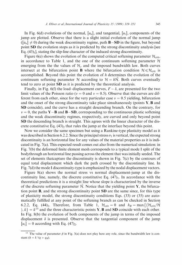
limit values of the Poisson ratio (� � 0 and � � 0:5). Observe that the curves are dif-ferent from each other, since for the very particular case � � 0:5 yielding, bifurcationand the onset of the strong discontinuity take place simultaneously (points Y;B andSD coincide), and the curve has a straight descending branch. On the contrary, for� � 0, the paths YÿB and BÿSD, corresponding to the continuous plastic softeningand the weak discontinuity regimes, respectively, are curved and only beyond pointSD the descending branch is straight. This agrees with the linear character of the dis-crete constitutive Eq. (43)2 that rules the jump at the interface beyond this point.Now we consider the same specimen but using a Rankine-type plasticity model as it

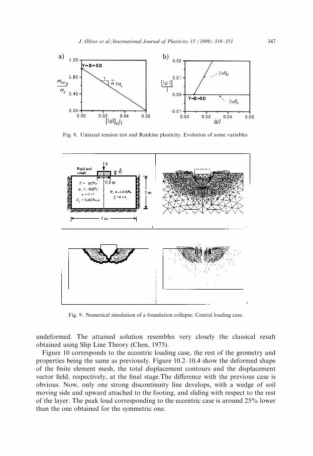
was described in Section 6.2.2. Since the principal stress�1 is vertical, the expected strongdiscontinuity is an horizontal line for any values of the material properties as it is indi-cated in Fig. 7(a). This expected result comes out also from the numerical simulation: inFig. 7(b) the deformed ®nite element mesh corresponds to a typical mode I split of thebodythrough an horizontal line passing across the element that was initially seeded. Theset of elements thatcapture the discontinuity is shown in Fig. 7(c) by the contours ofequal total displacement which dark the path crossed by the discontinuity line. InFig. 7(d) themode I discontinuity-type is emphasized by the nodal displacement vectors.Figure 8(a) shows the normal stress vs normal displacement-jump at the dis-

continuity line, namely, the discrete constitutive Eq. (47)1. In accordance with thetheoretical predictions it is a straight line whose slope is characterized by the inverseof the discrete softening parameter �H. Notice that the yielding point Y, the bifurca-tion point B, and the strong discontinuity point SD are the same since, for this typeof plasticity model, the strong discontinuity conditions Eqs. (33) or (35) are auto-matically ful®lled at any point of the softening branch as can be checked in Section6.2.2, Eq. (44)2. Therefore, from Table 1, Hcrit � 0 and hB � max Hcrit= �Hÿ��; kg � k15 and the three characteristic points Y;B and SD coincide with each other.In Fig. 8(b) the evolution of both components of the jump in terms of the imposeddisplacement � is presented. Observe that the tangential component of the jump��ut�� 0 according with Eq. (47)2.

15 The value of parameter � in Fig. 3(a) does not play here any role, since the bandwidth law is con-

stant (h � k 8q > qB).


11. Additional numerical simulations

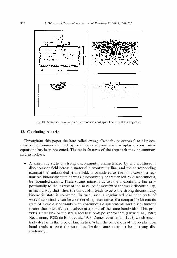
The numerical simulations presented in this Section correspond to the classicalgeomechanical problem of an undrained soil layer subjected to central or eccentricloading exerted by a rigid and rough surface footing. The same problem was con-sidered in reference (Zienckiewicz et al., 1995), where it was analyzed using anadaptive remeshing strategy to capture the formation of slip lines under perfectplasticity conditions. Here the problem is solved under plane strain conditions andusing a J2 plasticity model in the context of the strong discontinuity approach.Thebandwidth law is taken linear and such that � � 0:5. Geometry and results for thetwo cases analyzed are shown in Figs. 9 and 10. The ®nite element used in the dis-cretizations is a 6-noded quadratic triangle supplemented with the incompatibledisplacement referenced to in Section 9. Figure 9 corresponds to the central loadingcase. Figure 9.2 shows the deformed shape of the ®nite element mesh at the ®nalstage. In Fig. 9.3 the total displacement contours show the existence of two slipslines that initiate at the bottom corners of the footing and cross each other at acertain point of the symmetry axis. Figure 9.4 shows the displacement vector ®eld.From these it is clear that a triangular wedge of soil beneath the footing movessolidarily with this, vertically downward. This induces the upward movement of twolateral wedges that slide with respect the rest of the soil layer, which remains almost

Fig. 7. Uniaxial tension test and Rankine plasticity.


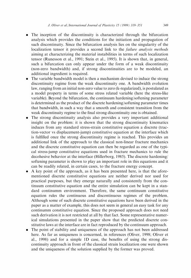
undeformed. The attained solution resembles very closely the classical resultobtained using Slip Line Theory (Chen, 1975).Figure 10 corresponds to the eccentric loading case, the rest of the geometry and

properties being the same as previously. Figure 10.2±10.4 show the deformed shapeof the ®nite element mesh, the total displacement contours and the displacementvector ®eld, respectively, at the ®nal stage.The di�erence with the previous case isobvious. Now, only one strong discontinuity line develops, with a wedge of soilmoving side and upward attached to the footing, and sliding with respect to the restof the layer. The peak load corresponding to the eccentric case is around 25% lowerthan the one obtained for the symmetric one.

Fig. 8. Uniaxial tension test and Rankine plasticity. Evolution of some variables.

Fig. 9. Numerical simulation of a foundation collapse. Central loading case.


12. Concluding remarks

Throughout this paper the here called strong discontinuity approach to displace-ment discontinuities induced by continuum stress-strain elastoplastic constitutiveequations has been presented. The main features of the approach may be summar-ized as follows:

. A kinematic state of strong discontinuity, characterized by a discontinuousdisplacement ®eld across a material discontinuity line, and the corresponding(compatible) unbounded strain ®eld, is considered as the limit case of a reg-ularized kinematic state of weak discontinuity characterized by discontinuous,but bounded strains. These strains intensify across the discontinuity line pro-portionally to the inverse of the so called bandwidth of the weak discontinuity,in such a way that when the bandwidth tends to zero the strong discontinuitykinematic state is recovered. In turn, such a regularized kinematic state ofweak discontinuity can be considered representative of a compatible kinematicstate of weak discontinuity with continuous displacements and discontinuousstrains that intensify (or localize) at a band of the same bandwidth. This pro-vides a ®rst link to the strain localization-type approaches (Ortiz et al., 1987;Needleman, 1988; de Borst et al., 1993; Zienckiewicz et al., 1995) which essen-tially deal with this type of kinematics. When the bandwidth of the localizationband tends to zero the strain-localization state turns to be a strong dis-continuity.

Fig. 10. Numerical simulation of a foundation collapse. Eccentrical loading case.


. The inception of the discontinuity is characterized through the bifurcationanalysis which provides the conditions for the initiation and propagation ofsuch discontinuity. Since the bifurcation analysis lies on the singularity of thelocalization tensor it provides a second link to the failure analysis methodsaiming at characterizing the material instabilities in terms of such localizationtensor (Runesson et al., 1991; Stein et al., 1995). It is shown that, in general,such a bifurcation can only appear under the form of a weak discontinuity(non-zero bandwidth) and, if strong discontinuities are to be modeled, anadditional ingredient is required.

. The variable bandwidth model is then a mechanism devised to induce the strongdiscontinuity regime from the weak discontinuity one. A bandwidth evolutionlaw, ranging from an initial non-zero value to zero (k-regularized), is postulated asa model property in terms of some stress related variable (here the stress-likevariable). Beyond the bifurcation, the continuum hardening/softening parameteris detetrmined as the product of the discrete hardening/softening parameter timesthat bandwidth, in such a way that a smooth and consistent transition from theweak discontinuity regime to the ®nal strong discontinuity one is obtained.

. The strong discontinuity analysis also provides a very important additionalinsight on the problem: it is shown that the strong discontinuity kinematicsinduces from any standard stress-strain constitutive equation a discrete (trac-tion-vector vs displacement-jump) constitutive equation at the interface whichis ful®lled once the strong discontinuity regime is reached. This provides anadditional link of the approach to the classical non-linear fracture mechanicsand the discrete constitutive equation can then be regarded as one of the typi-cal stress-jump constitutive equations used in fracture mechanics to rule thedecohesive behavior at the interface (Hillerborg, 1985). The discrete hardening/softening parameter is shown to play an important role in this equations and itcan be readily related, in certain cases, to the fracture energy concept.

. A key point of the approach, as it has been presented here, is that the afore-mentioned discrete constitutive equations are neither derived nor used forpractical purposes, but they emerge naturally and consistently from the con-tinuum constitutive equation and the entire simulation can be kept in a stan-dard continumm environment. Therefore, the same continuum constitutiveequation rules the continuous and discontinuous regimes of the problem.Although some of such discrete constitutive equations have been derived in thepaper as a matter of example, this does not seem in general an easy task for anycontinumm constitutive equation. Since the proposed approach does not needsuch derivation it is not restricted at all by that fact. Some representative numer-ical simulations presented in the paper show that the predicted discrete con-stitutive laws at the interface are in fact reproduced by the continuum approach.

. The point of stability and uniqueness of the approach has not been addressedhere. As far as uniqueness is concerned, in references (Oliver, 1998; Oliver etal., 1998) and for a simple 1D case, the bene®ts of using the strong dis-continuity approach in front of the classical strain localization one were shownand the uniqueness of the solution supplied by the former was proved.


Acknowledgements

The third author wishes to acknowledge the ®nancial support from the BrazilianCouncil for Scienti®c and Technological Development-CNPq.

References

Armero, F., Garikipati, K., 1995. Recent advances in the analysis and numerical simulation of strain

localization in inelastic solids. In: Owen, D., Onate, E., Hinton, E. (Eds.), Computational Plasticity.

Fundamentals and Applications, pp. 547-561.

Armero, F., Garikipati, K., 1996. An analysis of strong discontinuities in multiplicative ®nite strain plas-

ticity and their relation with the numerical simulation of strain localization in solids. Int. J. Solids and

Structures 33(20±22), 2863±2885.

Bazant, Z., Oh, B., 1983. Crack band theory for fracture of concrete. MateÂ riaux et Constructions 93(16),

155±177.

Chakrabarty, J., 1987. Theory of Plasticity. McGraw±Hill, New York.

Chen, J., 1975. Limit analysis and Soil Plasticity. Elsevier.

de Borst, R., Sluys, L. J., Muhlhaus, H. B., Pamin, J., 1993. Fundamental issues in ®nite element analyses

of localization of deformation. Engineering Computations 10, 99±121.

Dvorkin, E., Cuitino, A., Gioia, G., 1990. Finite elements with displacement embedded localization lines

intensive to mesh size and distortions. International Journal for Numerical Methods in Engineering 30,

541±564.

Hillerborg, A., 1985. Numerical methods to simulate softening and fracture of concrete. In: Sih, G. C., Di

Tomaso, A. (Eds.), Fracture Mechanics of Concrete: Structural Application and Numerical Calcula-

tion, pp. 141±170.

Khan, A., Huang, S., 1995. Continuum Theory of Plasticity. John Wiley & Sons.

Larsson, R., Runesson, K., Ottosen, N., 1993. Discontinuous displacement approximation for capturing

plastic localization. Int.J. Num. Meth. Eng. 36, 2087±2105.

Larsson, R., Runesson, K., Sature, S., 1996. Embedded localization band in undrained soil based on

regularized strong discontinuity theory and ®nite element analysis. Int. J. Solids and Structures 33(20±

22), 3081±3101.

Lee, H., Im., S., Atluri, S., 1995. Strain localization in an orthotropic material with plastic spin. Interna-

tional J. of Plasticity 11(4), 423±450.

Lofti, H., Ching, P., 1995. Embedded representation of fracture in concrete with mixed ®nite elements.

International Journal for Numerical Methods in Engineering 38, 1307±1325.

Lubliner, J., 1990. Plasticity Theory. Macmillan.

Needleman, A., 1988. Material rate dependence and mesh sensitivity in localization problems. Comp.

Meth. Appl. Mech. Eng. 67, 69±85.

Needleman, A., Tvergard, V., 1992. Analysis of plastic localization in metals. Appl. Mech. Rev. 45, 3±18.

Oliver, J., 1995a. Continuum modelling of strong discontinuities in solid mechanics. In: Owen, D. R. J.,

Onate, E., (Eds.), Computational Plasticity. Fundamentals and Applications, vol. 1. Pineridge Press,

pp. 455±479.

Oliver, J., 1995b. Continuum modelling of strong discontinuities in solid mechanics using damage models.

Computational Mechanics 17(1±2), 49±61.

Oliver, J., 1996a. Modeling strong discontinuities in solid mechanics via strain softening constitutive

equations. Part 1: fundamentals. Int. J. Num. Meth. Eng. 39(21), 3575±3600.

Oliver, J., 1996b. Modeling strong discontinuities in solid mechanics via strain softening constitutive

equations. Part 2: numerical simulation. Int. J. Num. Meth. Eng. 39(21), 3601±3623.

Oliver, J., 1998. The strong discontinuity approach: an overview. In: Idelsohn, S., Onate, E., Dvorkin, E.

N. (Eds.), Computational Mechanics. New Trends and Applications. Proceedings (CD-ROM) of the IV

World Congress on Computational Mechanics (WCCM98). CIMNE, pp. 1±19.


Oliver, J., Cervera, M., Manzoli, O., 1997. On the use of J2 plasticity models for the simulation of 2D

strong discontinuities in solids. In: Owen, D., Onate, E., Hinton, E. (Eds.), Proc. Int. Conf. on Com-

putational Plasticity, Barcelona, Spain. CIMNE, pp. 38±55.

Oliver, J., Cervera, M., Manzoli, O., 1998. On the use of strain-softening models for the simulation of

strong discontinuities in solids. In: de Borst, R., van der Giessen, E. (Eds.), Material Instabilities in

Solids, John Wiley & Sons, pp. 107±123 (Chapter 8).

Ortiz, M., Quigley, J., 1991. Adaptive mesh re®nement in strain localization problems. Comput. Methods

Appl. Mech. Engrg. 90, 781±804.

Ortiz, M., Leroy, Y., Needleman, A., 1987. A ®nite element method for localized failure analysis. Comp.

Meth. Appl. Mech. Eng. 61, 189±214.

Ottosen, N., Runesson, K., 1991. Properties of discontinuous bifurcation solutions in elasto-plasticity.

Int. J. Solids and Structures 27(4), 401±421.

Rots, J.G., Nauta, P., Kusters, G.M.A., Blaauwendraad, J., 1985. Smeared crack approach and fracture

localization in concrete. Heron 30(1), 1±49.

Runesson, K., Mroz, Z., 1989. A note on nonassociated plastic ¯ow rules. International J. of Plasticity 5,

639±658.

Runesson, K., Ottosen, N.S., Peric, D., 1991. Discontinuous bifurcations of elastic-plastic solutions at

phase stress and plane strain. Int. J. of Plasticity 7, 99±121.

Runesson, K., Peric, D., Sture, S., 1996. E�ect of pore ¯uid compressibility on localization in elastic-

plastic porous solids under undrained conditions. Int. J. Solids Structures 33(10), 1501±1518.

Simo, J., Oliver, J., 1994. A new approach to the analysis and simulation of strong discontinuities. In:

Bazant, Z.B., Bittnar, Z., JiraÂ sek, M., Mazars, J. (Eds.). Fracture and Damage in Quasi-brittle Struc-

tures. E & FN Spon, pp. 25±39.

Simo, J., Oliver, J., Armero, F., 1993. An analysis of strong discontinuities induced by strain-softening in

rate-independence inelastic solids. Computational Mechanics 12, 277±296.

Stein, E., Steinmann, P., Miehe, C., 1995. Instability phenomena in plasticity: modelling and computa-

tion. Computational Mechanics 17, 74±87.

Steinmann, P., Willam, K., 1994. Finite element analysis of elastoplastic discontinuities. Journal of Engi-

neering Mechanics 120, 2428±2442.

Zienckiewicz, O., Huang, M., Pastor, M., 1995. Localization problems in plasticity using ®nite elements

with adaptive remeshing. Int. J. Num. Anal. Meth. Geomech. 19, 127±148.


strong discontinuities and continuum plasticity models...

Documents