NASA TECH N I CA L NOTE ^i^QP| JNASA B DJ285 ^S ^^i^^rw,, T^N^ ro,60 KIF2TLAND AF Bg I ^’

Ln ^^^- ^

^ B g

^ ^ i-St

STRATEGIES FOR ESTIMATINGTHE MARINE GEOID FROM ALTIMETER DATA

P. Argentiero, W. D. Kahn, and R. Garza-Robles

Goddard Space Flight Center ^\\,i W~S^

Greenbelt, Md. 20771 \wf/’- / ’^e-ia16

NATIONAL AERONAUTICS AND SPACE ADMINISTRATION WASHINGTON, D. C. JULY 1976

I

https://ntrs.nasa.gov/search.jsp?R=19760022698 2019-04-03T20:53:35+00:00Z

TECH LIBRARY KAFB, NM

D1340S41. Report No. 2. Government Accession No. 3. Recipient’s Catalog No.NASA TN D-8285

4. Title and Subtitle 5. Report Date

Strategies for Estimating the Marine Geoid from July 1976Altimeter Data 6- ^’^’"""a Organization Code

9327. Author(s) 3. Performing Organization Report No.

P. Argentiero, W. D. Kahn and R. Garza-Robles G-76839. Performing Organization Name and Address 10. Work Unit No.

681-02-01-03_______Goddard Space Flight Center n- c0"*""^ G"" No.

Greenbelt, Maryland 20771 ,,13. Type of Report and Period Covered12. Sponsoring Agency Name and Address

National Aeronautics and Space Administration Technical NoteWashington, D.C. 20546 ,.

14. Sponsoring Agency Code

15. Supplementary Notes

16. Abstract

In processing altimeter data from a spacecraft-bome altimeter to estimate the finestructure of the marine geoid, a problem is encountered. To describe the geoid fine

structure, a large number of parameters must be employed, and to estimate all ofthem simultaneously is not possible. In practice, one is forced to hold a largenumber of parameters at a priori values and adjust others. Unless the parameteriza-tion exhibits good orthogonality in the data, serious aliasing results. Simulationstudies show that, among several competing parameterizations, the mean free-airgravity anomaly model (i.e., Stokes’ formula) exhibited promising geoid recoverycharacteristics.

Using covariance analysis techniques, this document provides quantitative measuresof the orthogonality properties associated with the previously mentioned parameteri-zation. For instance, a 5- by 5-degree area mean free-air gravity anomaly can beestimated with an uncertainty of 0.01 mm/s2 (1 mgal) (40-cm undulation) if allfree-air gravity anomalies within a spherical radius of 10 arc degrees are simultane-ously estimated.

17. Key Words (Selected by Author(s)) 18. Distribution Statement

Altimeter, Marine geoid, Unclassified-UnlimitedGravity anomalies

Cat. 4619. Security Classit. (of this report) 20. Security Clossif. (of this page) 21. No. of Pages 22. Price*

Unclassified Unclassified 27 $3.75

For sale by the National Technical Information Service, Springfield, Virginia 22161

This document makes use of international metric units according to theSysteme International d’Unites (SI). In certain cases, utility requires theretention of other systems of units in addition to the SI units. The conven-

tional units stated in parentheses following the computed SI equivalents are

the basis of the measurements and calculations reported.

CONTENTS

Page

ABSTRACT i

INTRODUCTION 1

SKYLAB AND GEOS-C ALTIMETER EXPERIMENTS 2

DESCRIPTION OF ALTIMETER MEASUREMENT 4

ORTHOGONALITY AND ALIASING 15

ESTIMATION STRATEGIES FOR GRAVITY ANOMALYDETERMINATION 20

SUMMARY 24

ACKNOWLEDGMENT 25

REFERENCES 27

iii

STRATEGIES FOR ESTIMATING THE MARINEGEOID FROM ALTIMETER DATA

P. ArgentieroW. D. Kahn

R. Garza-RoblesGoddard Space Flight Center

Greenbelt, Maryland

INTRODUCTION

The primary function of the spacecraft-borne altimeter is to determine the fine structure ofthe mean sea-surface topography. The instrument is well suited for the task. Consider, forinstance, the altimeter on board the Geodetic Earth-Orbiting Satellite-C (GEOS-C) spacecraftwhich was launched in late 1974. In its global mode, the instrument is capable of producinga measurement every 4 kilometers along the subearth path of the satellite. This impliesthat, even assuming considerable data compression, it will be mathematically possible toextract topographic detail of 1 degree or less from such data.

But practical difficulties must be overcome before the full potential of altimetry as a datatype can be realized. To determine these difficulties, standard estimation techniquesused to obtain sea-surface topography from altimetry data must be closely analyzed. Essen-tially, the problem is to reconstruct an analytic surface from direct but noisy observationsof the surface taken at specified points. The obvious approach is to parameterize the surfacein terms of coefficients which define a suitably dense set of functions in the space of twodimensional analytic functions and to recover the coefficients from the data by means of a

standard minimum variance filter. The physical setting of the problem often suggests theproper parameterization. If not, an arbitrary family of analytic functions such as the set oftwo dimensional polynomials can be used. For this problem, a natural parameterization is

suggested by the fact that, after suitable corrections, the mean sea surface can be consideredas cohering closely to an equipotential surface known as the marine geoid (Reference 1).Thus, one candidate for a natural parameterization is the set of standard spherical harmoniccoefficients of the Earth’s geopotential field.

Any parameterization capable of describing the fine structure of the surface in question mustemploy an enormous number of coefficients. For instance, determinization of 3-degreefeatures of the marine geoid using the standard spherical harmonic expansion of the geopo-tential field as a parameterization would require a full set of coefficients up to degree andorder 60. This implies the estimation of over 3700 parameters. Unless special circumstancesapply, it is impossible to simultaneously estimate such large parameter sets. In practice,

iiiiiiiiriiiii

to use parameter estimation techniques in recovering the marine-geoid fine structure from

altimeter data, it will be necessary to adjust small subsets of the parameters while "freezing"

the rest at a priori values. But, unless the parameterization exhibits a certain property with

regard to altimetry data which is termed "orthogonality in the data set," uncertainties in

the adjusted terms will badly corrupt the estimates of the adjusted terms. This effect is fre-

quently called aliasing. The orthogonality property just mentioned (defined in detail in a

later section) is a property of a parameterization which permits a decomposition of the esti-

mation problem into estimation problems of much smaller dimensionality without fear of

serious aliasing.

To take full advantage of the attractive properties of altimetry, it is necessary to develop a

parameterization of the marine geoid which exhibits good orthogonality properties in altim-

eter data. The orthogonality properties of the set of spherical harmonic coefficients of the

geopotential field are poor and are not good candidates for the proper parameterization.

Other candidates for the parameterization of the marine geoid are surface density layers

(Reference 2) and sample functions (Reference 3). The parameterization whose properties

are investigated in this paper is the one provided by mean free-air gravity anomalies and Stokes’

formula (References 4 and 5). If this parameterization is used to determine the marine geoid

from altimeter data, it is important to determine to what extent mean free-air gravity

anomalies are orthogonal in the data. Specifically, the important factor is how far two

mean free-air gravity anomalies must be separated to ensure that neglecting one anomaly

does not badly alias the estimate of the other. Without knowledge of this distance, intelligent

use of the parameterization is impossible.

Results of the Skylab altimeter experiment have demonstrated the ability of altimetry to re-

veal marine-geoid fine structure. However, the GEOS-C mission will provide the first oppor-

tunity for scientists to examine the output of a spacecraft-borne altimeter functioning in a

global mode over the oceans of the world. The next section details the performance of the

Skylab altimeter and the goals of the GEOS-C experiment. The mathematical details of

the measurement modeling and preprocessing of altimeter data will be described in a later

section, and the Stokes’ formula mean free-air gravity anomaly parameterization of the

marine geoid will be documented. Following that will be a detailed discussion of the dual

concepts of orthogonality and aliasing and their relationships to the problem of estimating

a marine geoid from altimeter data. Finally, the results of a systematic application of co-

variance analysis will be used to develop optimal estimation strategies for determining the

marine geoid from altimetry data.

SKYLAB AND GEOS-C ALTIMETER EXPERIMENTS

The GEOS-C spacecraft was inserted into orbit during the latter part of calendar year

1974. The prime experiment of this spacecraft was a radar altimeter. The objectives of

the GEOS-C altimeter experiment were: (a) to determine the feasibility and utility of a

spacebome altimeter to map the topography of the ocean surface with an absolute height

accuracy of +/-5 meters and with a relative height accuracy of 1 to 2 meters; (b) to

determine the feasibility of measuring the deflections of the vertical at sea; (c) to determine

2

the feasibility of measuring wave height; and (d) to contribute to technology leading to afuture operational satellite-altimeter system with a 10-cm measurement capability.

When calibrated and corrected (e.g., for sea state, ocean tides, and other effects), the altimeterdata constitute measures of the distance between the GEOS-C spacecraft and the ocean sur-face. Knowledge of the satellite altitude relative to a reference ellipsoid and knowledge of theoceanographic departures of the sea-surface topography from the geoid will then permit thedetermination of the geoid. The chief problem expected is the determination of orbitalaltitude for GEOS-C. The primary tracking systems for doing this are the satellite-to-satellitetracking system and precision lasers. Data from these and other systems tracking GEOS-C,including C-band radars, USE range and range-rate stations, and TRANET Doppler stations,will be used to find satellite height.

Satellite contributions to the determination of the current ocean geoid have spatial resolutionscorresponding to half wavelengths of approximately 18 degrees (2000 km). Although surfacegravity achieves representations with finer resolution, in the 1- to 5-degree (1 10- to 550-km)range, it covers only about 50 percent of the ocean surface. The GEOS-C altimeter systemwill therefore fill in the gaps and provide valuable independent knowledge where data nowexist.

The Skylab altimeter has recently demonstrated the ability of a radar altimeter to detectfeatures of the ocean surface. Figure 1 is an analysis of an altimeter pass over the PuertoRican Trench. The pass was over the southwest corner of Puerto Rico and was 72.8 second’sin duration. A plot of the height residuals (formed by comparing the altimeter measure-ments with the calculated height of Skylab’s orbit) shows that a 17-meter drop in heightresiduals occurred when Skylab passed over the deepest part of the ocean (i.e., correspondingto a 4000-meter depth of the ocean bottom) and that the peaking of the height residualsoccurred when Skylab traversed the Puerto Rican land mass. The Skylab data describedhere exemplify the high level of resolution of surface features by a radar altimeter.

Note, however, that data from the GEOS-C experiment will be significantly free of effectsof spacecraft dynamic motions, (which is not the case for Skylab altimeter data because ofattitude-control jet thrusting, crew motion, etc.). In addition, because GEOS-C had a nomi-nal 1-year operating lifetime, the altimetry data obtained was far greater than that obtainedfrom Skylab. For reasons previously cited, the GEOS-C altimeter experiment data are moresuitable for improving the marine geoid.

To successfully use GEOS-C altimetry data for improving the accuracy of the marine geoid,the development of unique computer programs capable of processing these data was neces-sary. The following sections describe the mathematical models associated with these pro-grams and the computation strategies for processing altimeter data.

3

(BEGIN PASS)

20

<^--4000.(--^p^^ C^

^^^^\ PUERTO ,3t r, RICO f\- 18 LJfc^-...-^---’5 .z . ^SKYLAB-1 MISSION ’. ^

ALTIMETER PASS No. 4 ’,(END PASS)

16 --------------[-----------------------290 291 292 293 294

E. LONGITUDE (DEG)

70

^^-- PUERTO RICANBEGINNING TIME: LAND MASS

6/4/73 171’ 15" 16.125 UT

END TIME:b 6/4/73 171’ 16" 28.92s UT

INTERVAL &T 72.8s40

5; 30

iL 20

5

10

-20TIME (SEC)

-3 __________I _L. ,1 ...J__ L__L -I0 5 10 15 20 25 30 35 40 45 50 55 60 65

Figure 1. Altimeter pass over the Puerto Rico Trench: (a) ground track

of altimeter pass; (b) Skylab-l altimeter residuals versus time data

source: NASA/Wallops Station.

DESCRIPTION OF ALTIMETER MEASUREMENT

Figure 2 shows the geometry associated with the altimeter measurement. As can be seen,

the altimeter measurement is nominally the shortest distance between the satellite and the

sea surface (i.e., the measurement is along the normal to the sea surface that passes through

4

UNCERTAINTY V ^^^ ""^^-^^^/ / ^SPACECRAFT (S/CI

INSTANTANEOUS / /h ^ V/iL ^^\SURFACE ’’ f /lt-*"\ ^^\ p ’"+\ // / ,-’ / / I " \ "ir-^.\ / ^^ ,’ / / \ |h| h,+8 h^ Ah

\ ^7 ~’4 ^,\ / / II \ BEAMVUIDTH h-N’-6h -Ah’>’ / / \s^ / / -^/-^ ANGLE

/ / / ^>C/ 7 WHERE:

/ r /flh-. 4/’^ Sfc, \ 7" S/C

/ ^’^. ./ .^ y~^^ST-----___l VECTOR FROM REFERENCE S/C^^. /I vTs~-^

/ l^/ ’1 ’^------’ GEOCENTRIC

^^^ / / jK \ ELLIPSOID.

^^---^^ (/ \ \ MAGNITUDE/ / ^^k- / \ Ns^ S/C ALTITUDE ABOVE SURFACE

\/^ / /I ^\,^ / ILLUMINATED \ HEIGHT ABOVE REFERENCE ELLIPSOID

/ .< / ^T^ F^O’T^R’INT 6h DEVIATION GEOID

/ /^/ / / ^s. Ah’ SYSTEMATIC ALTIMETER

/ / / \ \ MEASUREMENT, REFRACTION./ REFERENCE / \ \ OFFSET. TIMING,

/ ELLIPSOID /"

Figure 2. Altimeter measurement geometry.

the satellite). The following relationship gives the mathematical model for the altimeter

measurement:

h h- N’- Sh -Ah’ (1)

where

h l?-Tj

~^) position vector of S/C

T geocentric radius vector

N’ geoid height above reference ellipsoid

6h deviation of sea surface from geoid

Ah systematic errors in altimeter measurement (e.g., refraction, timing, etc.)

5

A more detailed description of the mathematical modeling of the altimeter measurement

appears in Reference 6.

The error sources that effect the altimeter measurement fall into three categories: (1) those

that result from orbit uncertainty; (2) those that cause the measured geoid to deviate from

the true geoid; and (3) those that affect the measurement accuracy itself. Equation 2 de-

scribes the functional dependence of the error sources on the altimeter measurement:

h^ h(^t) N’(Go) 5h,(?o^,0,X,t) Ah’(mo,0,X,t) (2)

where

h S/C altitude above reference ellipsoid

E orbit parameters and orbit dependent terms (radiation pressure, drag, etc.)

t time of altimeter measurement

^ vector of geopotential coefficients

N’ geoid undulation function

~! vector of tidal error model coefficients

T vector of local sea-surface biases (i.e., currents, storm surges, wind waves )

m vector of altimeter measurement error coefficients

or in general

\ h,(Eo,Go,?o,So,mo,<A,X,t) (3)

The altimeter measurement will be corrected for known error sources, smoothed, sorted,

etc., by the data preprocessor. Each measurement will then be compared with altitude cal-

culated from the satellite’s orbit (h^’) to form the measurement’s residual Ah^^a \ ^a (4)

Mathematically, this residual is equivalent to the difference function,

9ha ^a ^a VAh, -a- AE’ + -^- AGJ + -^ Ar^

BE, 3Gj 9r, (5)

8h, o 3h,+ -a. AS"+ Am’"+ e

3sg 3m^.

6

or

Ah^ Ah3(E) +Ah^(G) + Ah^(r) +Ah^(s) +Ah3(m) (5a)

Models for the altimeter measurement errors follow.

Error Attributable to Orbital Parameters (Aha (E))

Precision laser tracking, satellite-to-satellite tracking (SST), USE, C-band, and Doppler data

preceding and during altimeter measurement data acquisition will be used to correct theerror on altimeter measurements attributable to orbital parameters using an existing orbit-

determination program. Orbit-height accuracy required for altimetry data reduction must

be better than 1 meter. Recent studies indicate that this is feasible (Reference 7).

Error Attributable To Tides And Sea Surface (Ah (r) and Ah (S))

Corrections for deviations from the geoid attributable to ocean tides are based on the model

of Hendershott (Reference 8). This model represents the dominant lunar semidiurnal tide

(M ) with lunar declination terms neglected and is representative of the current state of the

art. The maximum error contribution attributable to tides is approximately meter. The

contributions attributable to local sea-surface biases are on the order of 50 cm, below the

resolution threshold of the GEOS-C altimeter. Therefore, sea-surface bias corrections are

neglected.

Errors Attributable To Altimeter Hardware (Ah (m))

Altimeter measurement errors which directly affect the accuracy for determining the geoidradius are:

Ah^(m) Ah;, + Ahg+Ah^ +Ahp +Ah^ +Ah^ (6)

where

Ah altimeter antenna offset

Ahg antenna offset due to S/C libration

Ah^ dynamic lag

Ahp altimeter drift

Ah^, timing bias

Ah^ tropospheric refraction

Models for the foregoing error sources follow.

7

Altimeter Antenna Offset

Aho \ tan V^ 8^) tan(ap 8^)

(cr)3 -/2/a,\

2

+ I--\ -.223 ff.-^\ \^) ( )

for

5b < "o < 2or

"(cr)3 ’72/ a^ 2

^ -.^ fc) -225

for

0 < "o < ^where

hg spacecraft altitude

5^ antenna half beamwidth angle

a,, angle off boresight

r transmitted pulse length

c velocity of light (299.7925 X 103 km/sec)

Antenna Offset Attributable to Spacecraft Libration

Ahg h^ tan ^(ag 6^) tan(ag 5^)

’(cr)3 172 / a \ 2

+ f - .225 (6c).^lA. .\25j

for

5,, < ag < 2

8

or

’(cr)3"72 / ae vAhg (-- } .22545gh,_ \25j (6d)

for

0 < ttg < 5,,

where

/27T \"c ^ ^" l-v- ^^e

Q’g S/C libration angle

Ag peak libration angle

0g libration phase angle

T orbital period

Dynamic Lag

Dynamic lag is a measurement-bias error induced by the change in spacecraft position at thetime of the outgoing and return pulses.

h- h,Ah, -^--1 jC

(ti.l ti) (6e)

where

hj altitude rate at time t. (sec)

lag coefficient (sec2)

9

Altimeter Drift

Altimeter drift is a measurement-bias error attributable to component aging.

Ahp D(t- tg) (6f)

where

t initial time of altimeter measurement

t current time of altimeter measurement

D drift coefficient (sec)

Timing Bias

Timing bias is bias error introduced by spacecraft clock error.

Ah^ hr (6g)

h height rate at time of altimeter measurement

r clock error coefficient

Tropospheric Refraction Error

Tropospheric refraction error is a bias error introduced into altimeter measurement becauseof tropospheric refraction. The model used is that developed by J. Saastamoinen (Reference 9).

Error Attributable to Geopotential A/7 (G)

In the preprocessing of altimeter data, the altimeter measurement will have been corrected forthe orbit uncertainties of ocean tides, local sea-surface biases, and measurement-bias errors

using the error models described previously. Thus equation 4 is restated as follows:

Ah^(G) \ [h^ + Ah^E) + Ah^(r) + Ah^(s) + Ahjm)] (7)

The relationship between altimeter measurement residuals to geoidal parameters can there-fore be stated as follows:

^aAh^G) ^^ AG,. (8)

3Gj

10

I

As stated previously, the altimeter measurement residual as described in Reference 7solely reflects primarily (neglecting second order effects) the departure of the .gepid fromthe reference ellipsoid or, more precisely, the distance along the unit normal to the refer-ence ellipsoid between the reference ellipsoid and the geoid which is called geoidal heightor geoidal undulation N’ (figure 2).

The mathematical relationship which relates the geoidal undulation to the disturbing poten-tial T is given by Bruns’ formula derived in Reference 4. That is,

TN (9)

7

where

T disturbing potential

7 magnitude of gravity vector normal to reference ellipsoid

The disturbing potential of the global geoid at point (0, X, r) is expressed in terms of sphericalharmonics as follows:

GM v- /a\" vT -7- L, (7) 2^ ^n^’" ^ [Cnm cos "^ + ^m sin mx! d)

n 2 m 0

where

GM gravitational constant of the earth

^m’ ^m spherical harmonic expansion coefficients

^m (sin ^ sssociated Legendre functions

(0, X) latitude and longitude on geoid at which disturbing potential is evaluated

r geocentric radius from earth center of mass to evaluation point of disturbingpotential on geoid

a semimajor azis of reference ellipsoid

L is the limit of summation, and it is specified by the degree of harmonicexpansion of the global geoid

n summation index for degree terms of the spherical harmonic expansionofT

m summation index for the order of terms in spherical harmonic expansionofT

11

Thus, the geoidal undulation at any point P (<f>, X, r) on the earth can be computed from geo-potential coefficients derived from satellites by analysis of perturbations on the orbits inducedby the Earth’s gravity field. The undulations are computed from the combination of equa-tions 9 and 10.

The Stokes’ formula (Reference 4, pp. 92-98) is another form of expressing the disturbingpotential. This formula makes it possible to express the disturbing potential of the globalgeoid from gravity data. That is,

T ^- ( Ag SW do (11)Jo J

where

a radius of reference ellipsoid

f flattening of reference ellipsoid

S (V/) Stokes’ function

a element of area

Ag surface gravity anomalies

SW csc (-j- 6 sin + -6 cos ^ 3 cos ^ In (sin T- ^-sin2 ) (lla)

from Bruns’ formula (equation 9).

The geoidal undulation at any point P on the global geoid can be computed from Stokes’formula (equation 1). That is;

N f fAgSW do (lib)7 47r7 Ja J

In terms of geographical coordinates. Stokes’ function can be expressed as follows:

R r ^ r"/2N(0,X) f I Ag(0’,X’) S(V/) cos ^’d0’dX’ (lie)

47r7 \’= o ^-Tr^

12

where

do cos 0’d0’dX’

(0, X) latitude and longitude of the computation point

(0’X’) coordinates of the variable surface element o

V/ spherical distance between the computation point and variable surface element

V/ cos"1 [sin 0 sin 0’ + cos 0 cos 0’ cos (X X’)]

Ag(0’X’) free-air gravity anomaly at the variable point (0’X’)

7 mean value of gravity over Earth

To combine surface gravity data and geopotential information derived from gravity field per-

turbations acting on orbits of spacecraft, the Earth is divided into two areas (Reference 10),a global area (A^) and a local area (A^), surrounding the point P. Each gravity anomaly in

each area is also partitioned into two parts represented by Ag^ and Ag^ respectively, where

L n n

^s ^ S, S (n l) (-l) pnm(sin ^{cnm cos nx +snm sin mx} (lld)

n 2 m 0

The Ag value is defined as the remainder of the gravity anomaly. By partitioning the Earth

into two areas and the geoidal undulations into two components, equation c can there-

fore be rewritten as follows:

N(0,X) N^ + N^ (lie)

where

27T 7T/2N, Ag.(0’,X’)S(V/) cos 0’d0’dX’

47T7 ’O ’--nil

or

T

7

13

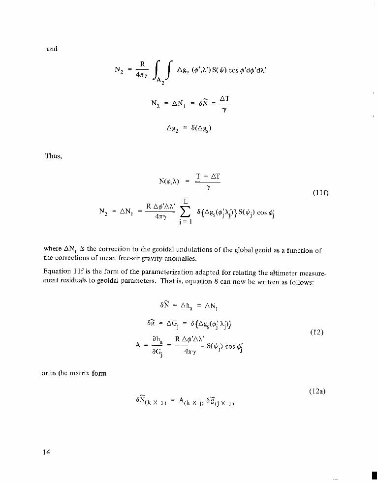
and

^ 7- 1 I Ag, (^>’,X’) SW cos 0’d0’dX’47T7 J j"-2

N- AN, 5N -7̂Ag^ 5(Ag,)

Thus,

T + ATN(0,\)

7(110

R AA’AX’ t-^

^ AN, --^-- S 5{Ag^Aj)}S(^) cos 0jJ

where AN^ is the correction to the geoidal undulations of the global geoid as a function ofthe corrections of mean free-air gravity anomalies.

Equation If is the form of the parameterization adapted for relating the altimeter measure-ment residuals to geoidal parameters. That is, equation 8 can now be written as follows:

5N Ah. AN,

5g AG, 5{Ag ^’ X’)}(12)

3h R A0’AX’A S(V/p cos 0;9G, 47T7

or in the matrix form

(12a)

^(k X l) ^k X j) 5^ l)

14

I

ORTHOGONALITY AND ALIASING

Assuming that altimeter observations can be directly translated into deviations of the marinegeoid from a reference geoid, it is straightforward to estimate gravity anomalies from altim-etry data. Let 5N be a vector of geoid undulations collected from a certain region over theocean. Next, let 5’gbe a vector of mean free-air gravity anomalies defined over a region ofthe ocean which contains the data region. Then, repeating equation 12,

5N A 5i (13)

where A is a matrix the number of whose rows is equal to the number of data points and thenumber of whose columns is equal to the number of gravity anomalies. As demonstratedin equation 12, the individual elements of A (for example, A (I, J)) can be computed throughStokes’ formula and the latitude and longitude of the i* data point, together with the longi-tude and latitude of the midpoint of the grid over which the J^ gravity anomaly is defined.Equation 13 provides a linear equation of condition, and, in a standard minimum variancefashion, g’could be estimated from observations of 5N. However, in order for equation 13to be correct (correct, that is, assuming that the approximations inherent in the discreteform.of Stokes’ formula are valid), the gravity anomalies in the array 5’g must cover theglobe. Considerably smaller regions would no doubt be adequate, but just how small theseregions can be before a serious bias is introduced into the estimation process must be deter-mined by computations. In any case, computational considerations necessitate the choiceof a region in which the number of elements in the 5^array does not exceed two or threehundred. Gravity anomalies outside this region are assumed to be zero. To see preciselywhat happens when this assumption is made, postulate that the 5gf array of equation 13 isdefined over an area so large that equation 13 is substantially correct. Then write

~5ii~5g

_g2 (14)

where

5g^ gravity anomalies to be adjusted in a standard minimum variance filter

and

Sg^ gravity anomalies assumed to be zero and thus left unadjusted by the minimumvariance filter.

Then equation 13 can be written

5N AI 5f; + A^ 51;, (15)

15

where A, and A^ are the variational matrices of 5N with respect to 5g, and with respect

to 5g, respectively.

After proper corrections, altimeter data are treated as direct observations 8N of 5N with

statistics

6N 5N + ^, E(iQ ^ 0, E(w1’) Q(16)

Estimates of mean free-air gravity anomalies obtained from satellite tracking and gravimetry

measurements are available (Reference 10). Unless this information was correctly factored

into the gravity anomaly estimates obtained from altimeter data, the resultant estimates

would not be optimal. Consequently, we assume the existence of an a priori estimate

5g, of 5g, with properties

5g’i 5gi +c^, E (ap 0, E (a, oi[) P^ ^For computational reasons, the gravity anomalies 5g^ are assumed to be zero, but actual

values of gravity anomalies in the region on the sphere which is ignored have a certain distri-

bution about zero. We assume

E (5g,) 0, E (5g2 5g^) P^ (18)

When the values of 5g^ are assumed to be zero, the minimum variance estimate of 5g^ be-

comes

5g, (A^ Q-1 A, + P^1)-1 [A^ Q-1 5N + P^ 5g’J

^See Reference for details. Define the covariance matrix of the estimator given by equation

19 as

P E [(5^ 5g^) (5gl 5g\)T] (20)

From equations 15, 16, 17, and 19, we obtain

5g, 5gi (A{ Q-1 AI + P,-1)-1 (-A[ Q-1 A, 5g, + A^~ Q-1 v + P^ ^) (21)

Equation 21 yields

P (A^Q^A, + P^1)-1 + (A{Q-lAlP-ll)-l A^Q-^P^Q-^

(A^’Q-^i + Pi1)-1

16

Assume that the data is Uncorrelated and that each data point has the same variance. Then

Q loji (23)

where I is the identity matrix and o^ is the common variance of the data. Also assume thatthe values of the unadjusted gravity anomalies are independently distributed. Then the co-variance matrix P^ of 5g^ can be written as

’ ^ 1p 02 0 (24)

^ 2.

where n^ is the number of unadjusted gravity anomalies and o?is the second moment aboutzero of the i^ unadjusted gravity anomaly.

Also define a matrix K as

K (A^Q-^i + P^1)-1 A^Q-^ (25)

If n^ is the number of adjusted parameters, then K is of dimension n^ by n^. With theseassumptions, equation 22 yields the following expression for the variance of the \*1 adjustedgravity anomaly

P(U) ^ (^, o.^j 0 (26)

where |3?^

is the i* diagonal element of matrix (A^A )’1 (assume here that diagonal elementsof matrix P"^ are relatively small) and

^ K(I,J), J > (27)

Define the error-sensitivity matrix as

s {^j}’ 1’2’-"r J 0,1,2,....^ (28)

and, finally, define the alias matrix as

L so (29)

17

where

~00a, 0

^2 (30)

a0

^The alias matrix reveals much of the probability structure of the estimation procedure.

Equations 26, 28, 29, and 30 show that the standard deviation of the i* adjusted gravity

anomaly is the root sum square (RSS) of the terms in the 1th row of the alias matrix. The

elements in the first column of the alias matrix represent the RSS contribution to the stan-

dard deviation of each estimated parameter caused by the data noise. The elements in the

J" column, J > 2, represent the RSS contribution to the standard deviation of each esti-

mated parameter attributable to the J !" unadjusted parameter. These terms are called

the aliasing contributions to the uncertainty in the adjusted parameters attributable to the

uncertainty in the J 1" unadjusted parameter. Note that the aliasing contributions attri-

butable to the 1th unadjusted parameter are proportional to the standard deviation of the

1th parameter. Definition: In a given estimation process, the Ith estimated parameter is

said to be orthogonal with respect to the 3th unestimated parameter if the aliasing contri-

bution to the Ith estimated parameter attributable to the uncertainty of the 1th unestimated

parameter is zero.

Two things can be noted about this definition. First, the orthogonality relationship between

two parameters must be defined within the context of a given estimation process. The

data set must be defined, and it must be stipulated which parameters are in the adjusted

and the unadjusted modes. Second, although the discussion has been of mean free-air

gravity anomalies and altimeter data, the mathematical results and definitions are applicable

to any linear estimation problem in which some parameters are adjusted and others are

left unadjusted.

To see the implications of the orthogonality relationship, a more revealing representation of

the aliasing terms is necessary. First, note that the first term on the right side of equation

22 is the covariance matrix of the estimation process under the assumption that the un-

adjusted parameters are perfectly known. This covariance matrix gives the uncertainty of

the estimates attributable to data noise only. Define the so-called "noise-only" covariance

matrix as

P (A]Q-lA, +^)-l (31)

18

Next, observe that the elements in the 1th row and 1th column of A and A respectively,are the partial derivative of the Ith data point with respect to the 1th adjusted parameter andthe partial derivative of the 1th data point with respect to the 3th unadjusted parameter. Thealiasing contribution to the 1th adjusted parameter attributable to the J^ unadjusted parametercan be written as

n^ m

L(I,J + 1) ^ P(I,K) ^K L(32)

95N(L) 35N(L)96g,(K) "- (L;L)

36g,(J)

where m is the number of data points.

If the estimates of the adjusted parameters are relatively uncorrelated in the noise-onlycovariance matrix, equation 32 can be approximated by

m

W^ W) SQ-’(^) -- 03)1 ""Sl*^ 95g:>(J)

A sufficient condition for the left side of equation 21 to approximate zero is for the obser-vability patterns of 5g^ (I) and 5g^ (J) in the data to be virtually nonoverlapping. Up toabout 40 degrees, Stokes’ function rapidly attenuates with increasing values of sphericalradius (Reference 4). Hence, if the grids on which 5g^ (I) and g^ (J) are defined are suffi-ciently separated, the orthogonality relationship will be effectively satisfied and the estimateof 6g^ (I) will not exhibit aliasing from the uncertainty of 5g, (J). Conversely, if the gridon which 5g^ (I) was defined were in close proximity to grids whose gravity anomalies wereunadjusted, serious aliasing of the resultant estimate would be expected.

It should be clear then, that if the gravity anomalies are estimated in a block, the outer layersof the block contain gravity anomalies whose estimates will be badly aliased by the adjacentunadjusted parameters, and must therefore be discarded. However, the gravity anomalies ina sufficiently small inner core of the block may be adequately separated from the unadjustedparameters to be effectively orthogonal with respect to them. The estimates of these termswill presumably be of sufficient accuracy that they can be accepted. In effect, for everyblock of gravity anomalies that will be estimated, it will be necessary to construct a "bufferzone" several layers deep of gravity anomalies which surround the block. The new and largerblock of gravity anomalies must be simultaneously estimated, and the estimates of gravityanomalies in the buffer zone must then be rejected because of aliasing. To achieve anintelligent compromise between estimation accuracy and computational load, it is necessaryto determine the relationship between the depth of the buffer zone and the accuracy of theestimation procedure. The relationship will vary with grid size, computation radius, anddata density. The most convenient way to study the relationship is to use covariance analysis

19

techniques to generate alias matrices for several situations and to attempt generalizations

from the results. This is done in the following section.

ESTIMATION STRATEGIES FOR GRAVITY ANOMALY DETERMINATION

The accuracy with which a given gravity anomaly is estimated from altimeter data is a func-

tion of many parameters. It is, of course, dependent on the accuracy and density of altim-

eter data. As explained in the previous section, it is also dependent on the radial distance

between the estimated gravity anomaly and the nearest gravity anomaly which is in the un-

adjusted mode. This parameter is called the estimation radius. Another parameter, the

computation radius, is an important determinant of the accuracy of a gravity anomaly esti-

mation. The computation radius sets the maximum distance from a given grid element over

which data is to be processed in order to estimate the gravity anomaly defined on that grid

element. Estimation accuracy does not necessarily increase with increasing computation

radius. Note that, for a given estimation radius, the covariance matrix of a set of estimated

gravity anomalies is given by equation 22 as the sum of a matrix which is dependent only on

data uncertainty and a matrix which represents the aliasing effects from the unadjusted

parameters. With increasing computation radius, the elements of the first matrix must de-

crease, but, in general, the elements of the matrix which conveys the aliasing effects will

increase. This effect can be shown graphically by means of so-called aliasing maps. The

aliasing maps of figures 3 and 4 were made simultaneously in a covariance mode, a situation

in which the marine geoid was described by means of 2- by 2-degree gravity anomalies and

by assuming 12 altimeter observations for each grid, each with an uncertainty of meter.

In figure 3, the RSS contribution was mapped in milligalileos (mgal)* to the uncertainty in the

estimated gravity anomaly defined on the grid element in the lower left-hand corner when the

adjacent anomalies were assumed to be in an unadjusted mode and to have an a priori uncer-

tainty of 0.50 millimeters/sec2 (mm/s2) (50 mgal). The computation radius was 5 degrees.

Note that the aliasing contributions decrease with the distance between the unadjusted

parameter and the estimated parameter, demonstrating the inherent orthogonality property

of the gravity anomaly parameterization of the marine geoid. In figure 4, the computation

radius has been changed to 20 degrees, and the aliasing effect decreased much less radically.

To achieve an intelligent compromise between computational load and estimation accuracy,

it is necessary to determine the precise relationship between the accuracy of the estimate of

a given gravity anomaly and the estimation radius and computation radius employed in the

estimation procedure. To do this, it was assumed that altimeter data existed at a density of

three data points per 1- by 1-degree grid and that the uncertainty on the data was 1 meter.

It was also assumed that unadjusted gravity anomalies had a standard error about zero of

0.50 mm/s2 (50 mgal). This figure is conservative; a more realistic figure is 0.30 mm/s2(30 mgal) (Reference 12). No a priori estimate was assumed for estimated parameters. The

effect of unadjusted parameters out to a spherical radius of 45 degrees were included in the

*Throughout the text of this document, the measurement unit of milligalileo (mgal) has been converted

to a Standard International Unit of millimeters/sec2 (mm/s2). For convenience, the illustrations have

not been converted. The simple conversion is mgal =0.01 mm/s

20

0 0 0 0 0

2 0 0 0

2 Q O

2 2 2 2 2 2 2 0 0 0

3 2 2 2 2 2 2 2 2 0 0

3 3 3 3 2 2 2 2 2 2 0

4 3 3 3 3 3 3 2 2

5 4 4 4 3 3 3 2 2 2

5 5 4 4 4 4 3 2 2 2 2

6 6 6 5 5 4 3 3 2 2 2

8 8 7 6 5 5 3 3 3 2 2 2

10 10 9 8 6 5 4 3 3 2 2 2

18 19 14 9 7 6 4 4 3 3 2 2

31 26 19 10 8 6 5 4 3 3 2 2 2

31 18 10 8 6 5 4 3 3 2 2 2

Figure 3. Alias map for 2- by 2-degree grids and for 5-degreecomputation radius.

4 4 4 4 4 4 4 3 3 3 3 2 2 2---i---4 4 5 5 5 5 4 4 4 3 3 3 2 2 2

5 6 6 6 6 5 5 5 5 4 4 3 3 2 2

6 7 7 7 7 7 6 6 5 5 4 4 3 3 2

8 8 9 9 8 8 8 7 7 6 5 4 4 3 3

10 10 11 11 11 10 10 9 8 7 6 5 4 4 3

12 14 14 14 14 13 12 11 10 8 7 6 5 4 3

15 16 17 17 16 15 14 13 11 9 7 6 5 4 4

17 19 19 20 19 17 16 14 12 10 8 7 6 5 4

19 22 22 22 21 19 17 16 13 10 9 7 6 5 4

22 24 25 24 22 21 19 16 14 11 9 7 6 5 4

25 28 28 26 24 22 19 17 14 11 9 7 6 5 4

28 32 30 28 25 22 20 17 14 11 9 7 6 5 4

36 34 32 28 24 22 19 16 14 11 9 7 6 5 4

._^j 36 28 25 22 19 19 15 13 10 8 7 6 5 4

Figure 4. Alias map in mgals for 2- by 2-degree grids and for20-degree computation radius.

21

computations. Under these conditions, figure 5 provides the standard deviation in the

estimates of 5- by 5-degree mean free-air gravity anomalies as a function ot estimation

radius and computation radius. This figure shows that the most efficient estimation strat-

egy for 5- by 5-degree anomalies is obtained with an estimation radius of about 10 degrees

and a computation radius of about 5 degrees. This strategy will result in an accuracy of

0.01 mm/s2 (1 mgal). This implies that if 5- by 5-degree mean free-air gravity anomalies

are estimated in blocks, estimates of gravity anomalies in the outer two layers of the block

should be discarded because of aliasing. The rest of the estimated gravity anomalies should

be accurate to within 0.01 mm/s2 (1 mgal), provided a 5-degree computation radius is

used. It is important to remember, however, that the prime intent is to estimate a marine

geoid rather than gravity anomalies. With estimates of 5- by 5-degree mean free-air gravity

anomalies. Stokes’ formula can be used to analytically reconstruct a marine geoid which is

sufficiently detailed that 5-degree features can be noted. Because the discrete form of

Stokes’ formula is linear, it is easy to propagate a given error in gravity-anomaly estima-

tion into an error in marine-geoid determination. Assuming that Stokes’ formula is accurate

if its summation is carried out within a 90-degree spherical radius of a given point, an 0.01-

mm/s2 (1-mgal) standard deviation in the estimate of 5- by 5-degree mean free-air gravity

anomalies propagates into a 40-cm standard deviation of the resultant marine geoid. There-

fore, by applying proper estimation procedures to the reduction of altimeter data, deter-

mination of 5-degree features of the marine geoid with a resolution of 40 cm should be

possible.

"\~~ I ASSUMPTIONS

Gravity milligals

Density 1" 1"

/ ioy / ^^ ^

________L L. 19" 11’ 13" 18 19’

Figure 5. Accuracy of 5- by 5-degree mean free-air gravity anomaly estimate versus compu-

tation radius for various estimation radii.

22

To obtain a more detailed marine geoid presents a more difficult estimation problem. Figure6 provides the standard deviation in the estimates of 3- by 3-degree mean free-air gravityanomalies as a function of estimation radius and computation radius. An estimation radiusof 12 degrees and a computation radius between 10 and 11 degrees appears to provide themost intelligent estimation strategy. The strategy leads to estimates of 3- by 3-degree meanfree-air gravity anomalies with standard deviations of 0.05 mm/s2 (5 mgal). This impliesthat, if 3-degree mean free-air gravity anomalies are estimated in blocks, the outer fourlayers must be discarded as being badly aliased. An 0.05-mm/s2 (5-mgal) standard deviationin estimates of 3- by 3-degree mean free-air gravity anomalies propagates into a standarddeviation of 1.2 m in the resultant marine geoid. With the present assumptions, no estima-tion strategy is adequate to determine features of the marine geoid as small as 2 degrees.With much greater data densities, such fine resolution is possible. For instance, if we in-crease the data density by a factor of 100, thus postulating 300 data points for each 1- by1-degree block, then, with an estimation radius of 10 degrees and a computation radius of2 degrees, 2- by 2-degree anomalies can be estimated with a standard deviation of 0.023mm/s2 (2.3 mgal). This propagates into a standard deviation of the marine geoid of about42 cm. However, it is probably not realistic to postulate such data densities, and, in addi-tion, it suggests a very heavy computational load. The accurate resolution of 3-degreefeatures of the marine geoid is likely to be the limit of what can be accomplished withaltimeter data and the Stokes’ formula mean free-air gravity anomaly parameterization ofthe marine geoid.

-^----------/

Gravity milligals

Density x1"

s’*^^ ~~~--"’^ ^ 12. 16", 18, 21"

1" 2 3 4 5 6" 7 8 9 10 11 12" 13 14 15 16 17 18 19 20 21 22

RADIUS

Figure 6. Accuracy of 3- by 3-degree mean free-air gravity anomaly estimate versus compu-

tation radius for various estimation radii.

23

Finally, note that these results were accomplished without assuming a priori estimates of

gravity anomalies. In fact, these estimates have been derived from satellite tracking data

and direct gravity measurements. When these estimates are optimally combined with

altimeter data by means of equation 10, the resultant estimates of gravity anomalies will be

predicted on all relevant data. The representation of the marine geoid derived from these

estimates will then constitute the best possible estimate of that surface.

SUMMARY

Data from the Skylab altimeter have demonstrated the ability of altimetry to discern the fine

structure of the marine geoid. However, during the GEOS-C mission, global sensing of

sea-surface topography from a spacecraft-borne altimeter will be possible for the first time.

To make optimal use of the vast amount of altimeter data expected from the GEOS-C,

numerous corrections must be made to the data, both to eliminate systematic errors inherent

in the data type itself and to correct for the effects of deviations of the mean sea surface

from the marine geoid.

To employ standard parameter-estimation techniques for estimating a marine geoid from

altimeter data, it is necessary to use a parameterization of the marine geoid which exhibits

good orthogonality characteristics in the data type. In this respect at least, the Stokes’ formula

mean free-air gravity anomaly parameterization appears to be the most promising. For a

given grid size and data density, the accuracy of the geoid resulting from an estimate of

gravity anomalies from altimeter data is a strong function of the choice of estimation radius

and computation radius. An application of covariance analysis techniques reveals that,

assuming a data density of three measurements per 1- by 1-degree spherical surface area with

each measurement accurate to within 1 meter, optimal choices of estimation radius and

computation radius of 10 and 5 degrees, respectively, yield an accuracy in the estimate of

5- by 5-degree mean free-air gravity anomalies of approximately 0.01 mm/s2 (1 mgal). This

result implies that, with a judicious choice of estimation strategy, geoid height can be deter-

mined with a standard deviation of 40 cm and a spatial resolution of 500 km (5 arc degrees).

With the same data density and data accuracy assumptions, covariance analysis demonstrates

that optimal choices of 12 degrees for estimation radius and 10 degrees for computation

radius permits one to estimate with an accuracy of approximately 1.2 m in geoid height with

a spatial resolution of 300 km (3 arc degrees). Severe aliasing difficulties are encountered in

attempting to estimate more detailed geoids. Our covariance analysis studies indicate, how-

ever, that a very small computation radius, together with great data densities, can mitigate

the aliasing effects and yield in localized areas a marine geoid capable of showing spatial

resolutions at the 100- to 200-km level.

Finally, note that use of the Stokes’ formula mean free-air gravity anomaly parameterization

of the marine geoid makes it easy to combine satellite tracking data and direct measurements

of gravity anomalies with altimeter data to obtain an optimal estimate of the marine geoid.

24

ACKNOWLEDGMENT

The authors wish to thank J. T. McGoogan of NASA/Wallops Station for providing theSkylab altimeter data used in this report.

Goddard Space Flight CenterNational Aeronautics and Space Administration

Greenbelt, Maryland June 7,1976

25

I

REFERENCES

1. Greenwood, J. A., et al.. Radar Altimetry from a Spacecraft and its PotentialApplications to Geodesy and Oceanography, New York University School ofEngineering and Science, Department of Meteorology and Oceanography, Reporton Contract N62306-1589, U. S. Naval Oceanographic Office, May 1967.

2. Koch, K. R., and B. V. Witte, The Earth’s Gravity Field Represented by a SimpleLayer Potential from Doppler Tracking of Satellites, NOAA Technical Memoram-dum No. 59, April 1971.

3. Lundquist, C. A., G. E. 0. Giacaglia, K. Hebb, and S. G. Mair, Possible GeopotentialImprovement from Satellite Altimetry, Smithsonian Astrophysical Observatory,Report No. 294, 1970.

4. Heiskanen, W. A., and H. Moritz, Physical Geodesy, W. H. Freeman and Co., 1967.

5. Koch, K. R., Gravity Anomalies for Ocean Areas from Satellite Altimetry, Proceed-ings of the Second Marine Geodesy Symposium, Marine Technology Society,Washington, D. C., 1970.

6. Brown, R. D., and R. J. Fury, Determination of the Geoid from Satellite Altimeter,NASA TM X-66016, pp. 4-3-4-13, 1972.

7. Argentiero, P., and J. Lynn, Estimation Strategies for Orbit Determination, NASATM X-70610, 1974.

8. Hendershott, M. C., The Effects of Solid Earth Deformation on Global Ocean Tides,Geophys. J., R. Astr. Soc 29, pp. 389-402, 1972.

9. Saastamoinen, J.. "The Use of Artificial Satellites for Geodesy," pp. 247-251;Geophysical Monograph 15, AGU 1972, "Atmospheric Correction for the Trop-osphere and Stratosphere in Radio Ranging Satellites," 1972.

10. Marsh, J., and S. Vincent, A Global Detailed Geoid, NASA TM X-70492, 1973.

1 1. Deutch, Ralph, Estimation Theory, Prentice Hall, 1965.

12. Rapp, R. H., The Geoid Definition and Determination, Fourth GEOP Conference,University of Colorado, Boulder, August 1973.

NASA-Langley, 1976 27

1y ’\

NATIONAL AERONAUTICS AND SPACE ADMINISTRATION _^^^kWASHINGTON, D.C. 20546 -^^^fc>^f9^^

OFFICIAL BUSINESS ^^H.PENALTY *3oo SPECIAL FOURTH-CLASS RATE ggSBT

BOOK ^^^617 001 Cl U E 760702 S00903DSDEPT OF THE AI R FORCEAF WEAPONS LABORATORYATTN : TECHNICAL LIBRARY ( SUL)

KIRTLANO AFB NM 87117

If Undeliverable (Section 158POSTMASTER: postal Manual) Do Not Return

"The aeronautical and, space activities of the United States shall beconducted so as to contribute to the expansion of human knowl-edge of phenomena in the atmosphere and space. The Administrationshall provide for the widest practicable and appropriate dissemination

of information concerning its activities and the results thereof."--NATIONAL AERONAUTICS AND SPACE ACT OF 1958

NASA SCIENTIFIC AND TECHNICAL PUBLICATIONSTECHNICAL REPORTS: Scientific and TECHNICAL TRANSLATIONS: Information

technical information considered important, published in a foreign language considered

complete, and a lasting contribution to existing to merit NASA distribution in English.

knowledge.k A SPECIAL PUBLICATIONS: Information

TECHNICAL NOTES: Information less broadA

in scope but nevertheless of importance as a derived from or of value to NASA activities.

contribution to existing knowledge. Publications include final reports of ma,orprojects, monographs, data compilations,

TECHNICAL MEMORANDUMS: handbooks, sourcebooks, and specialInformation receiving limited distribution bibliographiesbecause of preliminary data, security classifica-

tion, or other reasons. Also includes conference TECHNOLOGY UTILIZATIONproceedings with either limited or unlimited PUBLICATIONS: Information on technologydistribution. yggj ^y NASA that may be of particularCONTRACTOR REPORTS: Scientific and interest in commercial and other non-aerospacetechnical information generated under a NASA applications. Publications include Tech Briefs,contract or grant and considered an important Technology Utilization Reports and

contribution to existing knowledge. Technology Surveys.

Details on the availability of these publications may be obtained from:

SCIENTIFIC AND TECHNICAL INFORMATION OFFICE

N AT O N A L A E R O N A U T C S A N D S P A C E A DM N S T RAT O N

Washington, D.C. 20546