Paper SAS521-2017

Step Up Your Statistical Practice with Today’s SAS/STAT® Software

Robert N. Rodriguez, Phil Gibbs, and Randy Tobias, SAS Institute Inc.

Abstract

Has the rapid pace of SAS/STAT® releases left you unaware of powerful enhancements that could make a difference in your work? Are you still using PROC REG rather than PROC GLMSELECT to build regression models? Do you understand how the GENMOD procedure compares with the newer GEE and HPGENSELECT procedures? When should you turn to PROC ICPHREG rather than PROC PHREG for survival modeling?

This paper will increase your awareness of modern tools in SAS/STAT by providing high-level comparisons with well-established tools and explaining the benefits of enhancements and new procedures. The paper focuses on new tools in the areas of regression model building, generalized linear models, survival analysis, and mixed models. When you see the advantages of these tools, you will want to put them into practice. The paper also points out resources that will guide you to new tools in other important areas, such as Bayesian analysis, causal inference, item response theory, methods for missing data, and survey data analysis.

Introduction

Are you a creature of habit when it comes to analyzing data? Do you still rely on PROC REG and PROC GLM for your regression studies because those are the procedures you learned about in school? Have you heard about recent releases of SAS/STAT and new procedures—but not found time to check them out? If so, the procedures that you know best might not be your best choices when compared with newer procedures that deliver significant advances in methodology. And you might not be aware of alternatives that could make a difference in your work.

This paper provides that awareness. Each of its four main sections focuses on an area where SAS/STAT has grown significantly in recent years:

� The section on “Regression Model Building” describes new tools for selecting the effects in your model when youhave many variables to choose from—continuous or categorical. You might be building traditional explanatorymodels if your goal is to gain insights. Or you might now be building predictive models if your goal is accurateprediction with new data. Either way, you can build better models by applying modern selection methods,such as the lasso, and you can build a broader range of models in which the response can be categorical orcontinuous.

� The section on “Inferential Analysis of Generalized Linear Models” describes new tools for different kindsof inference—such as estimation of treatment effects—within the framework of generalized linear models.These tools help you to take advantage of modern Bayesian methods, deal with overdispersion, and handlemissingness that is due to dropouts in longitudinal studies.

� The section on “Survival Analysis” describes new tools for estimation and hypothesis testing and for modeling theoutcome of interest when you have time-to-event data. These tools are indispensable for valid inference becausethey are specialized for particular problems that you encounter with right-censored data, interval-censored data,competing risks, and clustered data.

� The section on “Analysis of Mixed Models” describes the various procedures available in SAS/STAT softwarefor handling models with both fixed and random effects. Understanding how these tools compare in terms offlexibility and practical advantages will help you decide which ones to apply in your work.

Each section begins by noting the most familiar procedures in that area, and it then presents new tools—enhancementsand new procedures—that give you greater flexibility for statistical modeling, specialized inference for complex data,and improved performance for large data. The discussion compares the objectives, assumptions, and benefits of thenew tools.

Because this paper presents a high-level view, it does not include examples or explanations of methods. Instead, eachsection refers to introductory papers that cover these aspects. The final section points out resources that guide you tonew tools in areas of SAS/STAT software that are not covered here, such as Bayesian analysis, causal inference, itemresponse theory, methods for missing data, and survey data analysis.

1

Regression Model Building

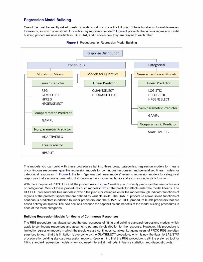
One of the most frequently asked questions in statistical practice is the following: “I have hundreds of variables—eventhousands, so which ones should I include in my regression model?” Figure 1 presents the various regression modelbuilding procedures now available in SAS/STAT, and it shows how they are related to each other.

Figure 1 Procedures for Regression Model Building

The models you can build with these procedures fall into three broad categories: regression models for meansof continuous responses, quantile regression models for continuous responses, and generalized linear models forcategorical responses. In Figure 1, the term “generalized linear models” refers to regression models for categoricalresponses that assume a parametric distribution in the exponential family and a corresponding link function.

With the exception of PROC REG, all the procedures in Figure 1 enable you to specify predictors that are continuousor categorical. Most of these procedures build models in which the predictor effects enter the model linearly. TheHPSPLIT procedure fits tree models in which the predictor variables enter the model through indicator functions ofregions of the predictor space that are defined by variable splits. The GAMPL procedure allows spline functions ofcontinuous predictors in addition to linear predictors, and the ADAPTIVEREG procedure builds predictors that arebased entirely on splines. The next sections describe the capabilities and benefits of the model building procedures ineach of the three categories.

Building Regression Models for Means of Continuous Responses

The REG procedure has always served the dual purposes of fitting and building standard regressions models, whichapply to continuous responses and assume no parametric distribution for the response. However, this procedure islimited to regression models in which the predictors are continuous variables. Longtime users of PROC REG are oftensurprised to learn that this limitation is overcome by the GLMSELECT procedure, which is now the flagship SAS/STATprocedure for building standard regression models. Keep in mind that the REG procedure is still the preferred tool forfitting standard regression models when you need inferential methods, influence statistics, and diagnostic plots.

2

A major advantage of PROC GLMSELECT over PROC REG is that it supports effect selection methods for generallinear models of the form

yi D ˇ0 C ˇ1xi1 C � � � C ˇpxip C �i ; i D 1; : : : ; n

where the response yi is continuous and the predictors xi1; : : : ; xip represent main effects that consist of continuousor classification variables, and interaction effects of these variables. You specify the model by using MODEL andCLASS statements as in the GLM procedure. By using the EFFECT statement, you can include more types ofeffects—such as polynomial and spline effects—that are constructed from the variables.

Another advantage of PROC GLMSELECT is that it provides lasso methods, introduced by Tibshirani (1996), inaddition to the forward, backward, and stepwise selection methods available in the REG procedure. Lasso methodsleave all the effects in the model, but they restrict their parameters by setting some to zero while shrinking otherstoward zero. Thus, they produce models that are sparser and potentially more interpretable (Hastie, Tibshirani, andWainwright 2015). Table 1 summarizes the selection methods available in the GLMSELECT procedure.

Table 1 Effect Selection Methods in the GLMSELECT Procedure

Method Description

Forward selection Starts with no effects and adds effectsBackward elimination Starts with all effects and deletes effectsStepwise selection Starts with no effects; effects are added and can be deletedLeast angle regression Starts with no effects and adds effects; at each step, estimated

ˇs are shrunk toward 0Lasso Constrains sum of absolute ˇs; some ˇs set to 0Elastic net Constrains sums of absolute and squared ˇs; some ˇs set to 0Adaptive lasso Constrains sum of absolute weighted ˇs; some ˇs set to 0Group lasso Constrains sum of Euclidean norms of ˇs corresponding to effects;

all ˇs for the same effect are set to 0 or are nonzero

The GLMSELECT procedure also provides extensive capabilities for customizing effect selection. You can specifyinformation criteria or criteria based on significance levels. You can also specify criteria based on validation; thisapproach avoids overfitting the training data by partitioning the data into subsets for training, validation, and testing.

To address the computational demands of selection from a very large number of effects, the GLMSELECT procedurehas added screening approaches that you can combine with selection methods to reduce the number of regressors toa smaller subset on which the selection is then performed.

Cohen (2006) provides an introduction to the GLMSELECT procedure, and Cohen (2009) describes its strengths forbuilding models with large data. Günes (2015) discusses regression methods based on penalization. Gibbs et al.(2013) explain the versatility of the EFFECT statement, which is available in many SAS/STAT modeling procedures.

The HPREG procedure is a high-performance procedure that has many of the same features as the GLMSELECTprocedure for fitting and building standard regression models. PROC HPREG is referred to as a high-performanceprocedure because it runs in either single-machine mode or distributed mode, and it is multi-threaded. Cohen andRodriguez (2013) describe the design of high-performance statistical modeling procedures and discuss when theseprocedures provide performance benefits.

The HPSPLIT procedure is a high-performance procedure that builds regression trees, which model continuousresponses, and classification trees, which model categorical responses. The predictor variables can be categoricalor continuous, and the tree is built by recursively splitting the predictor space into nonoverlapping segments, whichdefine the terminal nodes of the tree. The process begins by growing a large, full tree. To prevent overfitting, thefull tree is pruned back to a smaller subtree that balances the goals of fitting the training data and predicting newdata. The average response of the training observations in a terminal node serves to predict the response for newobservations that fall into that node.

An advantage of regression trees over standard regression models is that they are easy to explain; tree diagramscan be highly interpretable when the tree size is small. On the other hand, because regression trees lack flexibilityfor capturing smooth relationships between the predictors and the response, they often fail to provide the predictiveaccuracy of linear regression models.

3

Building Quantile Regression Models for Continuous Responses

The standard regression models that you build with the GLMSELECT and HPREG procedures predict the condi-tional mean of the response (EŒY jX�), and they assume that the conditional variance of the response is constant(VarŒY jX� D �2). Models of this type cannot describe data in which the shape of the response distribution dependson the predictors.

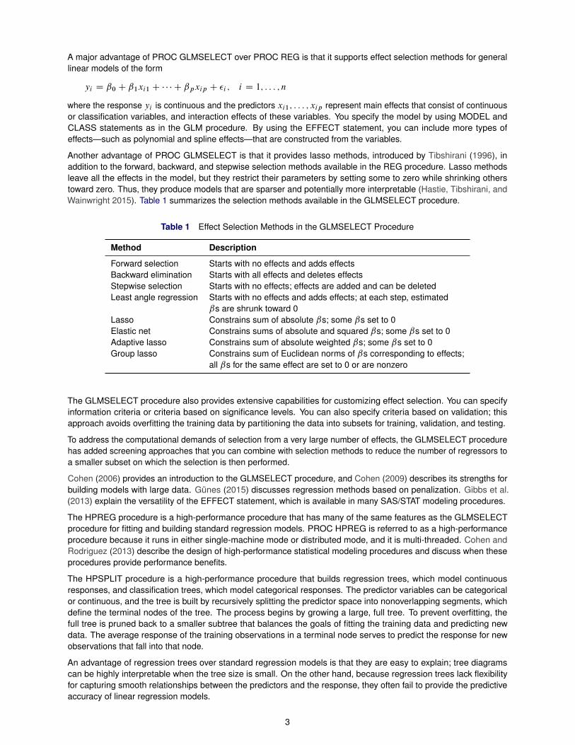
For example, consider the data shown in Figure 2, where the variance of Y increases with X. You can use a simplelinear regression model to predictEŒY jX�, but this model cannot account for the variation in the conditional distributionof Y.

Figure 2 Quantile Regression Models for Three Percentiles

Quantile regression, introduced by Koenker and Bassett (1978), uses a general linear model to fit conditionalquantiles—more commonly referred to as percentiles—of the response without assuming a parametric distribution forthe response. Figure 2 shows quantile regression lines for the 10th, 50th, and 90th conditional percentiles of Y, fittedwith the QUANTREG procedure. By fitting a more extensive set of percentiles, you can describe the entire conditionaldistribution of Y. When the shape of the conditional distribution varies nonlinearly with the predictors, you can includepolynomial or spline effects in the model.

Table 2 summarizes important differences between standard linear regression and quantile regression.

Table 2 Comparison of Linear Regression with Quantile Regression

Linear Regression Quantile Regression

Predicts the conditional mean EŒY jXŒ Predicts conditional quantiles Q� ŒY jX�Applies even with small data Needs sufficient dataCan assume normality Does not assume a parametric distributionSensitive to outliers Robust to outliersComputationally inexpensive Computationally intensive

For many years, quantile regression was impractical because its computational cost was too high when the number ofobservations was sufficiently large for accurate prediction of quantiles, especially in the tails. Today, however, quantileregression is quite practical—even for very large data—with the algorithms that are available in the QUANTREG andQUANTSELECT procedures. Quantile regression can reveal the effects of predictors on different parts of the responsedistribution, and it can yield valuable insights in applications such as risk management, where useful information liesin the tails.

The QUANTSELECT procedure performs effect selection for quantile regression. Like the GLMSELECT procedure, itis designed primarily for effect selection, and it offers similar methods of effect selection. The HPQUANTSELECTprocedure is a high-performance procedure that provides functionality similar to that of PROC QUANTSELECTfor building quantile regression models. See Rodriguez and Yao (2017) for applications of the QUANTREG andQUANTSELECT procedures.

4

Building Regression Models for Categorical Responses

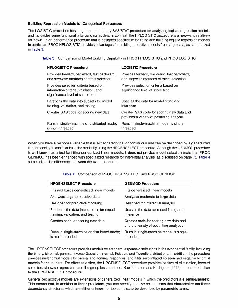
The LOGISTIC procedure has long been the primary SAS/STAT procedure for analyzing logistic regression models,and it provides some functionality for building models. In contrast, the HPLOGISTIC procedure is a new—and relativelyunknown—high-performance procedure that is designed specifically for fitting and building logistic regression models.In particular, PROC HPLOGISTIC provides advantages for building predictive models from large data, as summarizedin Table 3.

Table 3 Comparison of Model Building Capability in PROC HPLOGISTIC and PROC LOGISTIC

HPLOGISTIC Procedure LOGISTIC Procedure

Provides forward, backward, fast backward, Provides forward, backward, fast backward,and stepwise methods of effect selection and stepwise methods of effect selection

Provides selection criteria based on Provides selection criteria based oninformation criteria, validation, and significance level of score testsignificance level of score test

Partitions the data into subsets for model Uses all the data for model fitting andtraining, validation, and testing inference

Creates SAS code for scoring new data Creates SAS code for scoring new data andprovides a variety of postfitting analysis

Runs in single-machine or distributed mode; Runs in single-machine mode; is single-is multi-threaded threaded

When you have a response variable that is either categorical or continuous and can be described by a generalizedlinear model, you can fit or build the model by using the HPGENSELECT procedure. Although the GENMOD procedureis well known as a tool for fitting generalized linear models, it does not provide model selection (note that PROCGENMOD has been enhanced with specialized methods for inferential analysis, as discussed on page 7). Table 4summarizes the differences between the two procedures.

Table 4 Comparison of PROC HPGENSELECT and PROC GENMOD

HPGENSELECT Procedure GENMOD Procedure

Fits and builds generalized linear models Fits generalized linear models

Analyzes large to massive data Analyzes moderate to large data

Designed for predictive modeling Designed for inferential analysis

Partitions the data into subsets for model Uses all the data for model fitting andtraining, validation, and testing inference

Creates code for scoring new data Creates code for scoring new data andoffers a variety of postfitting analyses

Runs in single-machine or distributed mode; Runs in single-machine mode; is single-is multi-threaded threaded

The HPGENSELECT procedure provides models for standard response distributions in the exponential family, includingthe binary, binomial, gamma, inverse Gaussian, normal, Poisson, and Tweedie distributions. In addition, the procedureprovides multinomial models for ordinal and nominal responses, and it fits zero-inflated Poisson and negative binomialmodels for count data. For effect selection, the HPGENSELECT procedure provides backward elimination, forwardselection, stepwise regression, and the group lasso method. See Johnston and Rodriguez (2015) for an introductionto the HPGENSELECT procedure.

Generalized additive models are extensions of generalized linear models in which the predictors are semiparametric.This means that, in addition to linear predictors, you can specify additive spline terms that characterize nonlineardependency structures which are either unknown or too complex to be described by parametric terms.

5

The GAMPL procedure is a new high-performance procedure that fits generalized additive models by using low-rankregression splines (Wood 2003, 2006). PROC GAMPL does not provide effect selection, but it does produce plotsthat you can use to explore the additive effects of the spline components. These plots can suggest parametriceffects—such as quadratic polynomials—for models that you can then build with the HPGENSELECT procedure.

You might be familiar with the earlier GAM procedure for fitting generalized additive models. PROC GAMPL implementsnewer approaches, such as penalized likelihood estimation, a modified performance iteration method (Wood 2004)and the outer iteration method (Wood 2006). As a result, it provides greatly improved performance for large data.

The ADAPTIVEREG procedure fits response variables with distributions in the exponential family, including the binomial,gamma, inverse Gaussian, normal, negative binomial, and Poisson distributions. The predictor is nonparametricand is constructed from regression splines. The procedure is based on an approach due to Friedman (1991), whichconstructs spline basis functions in an adaptive way by automatically selecting appropriate knot values for differentvariables. The approach creates an overfitted model and then prunes it with backward selection. You can use theADAPTIVEREG procedure to model complex, unknown relationships between the predictors and the response. SeeKuhfeld and Cai (2013) for an introduction.

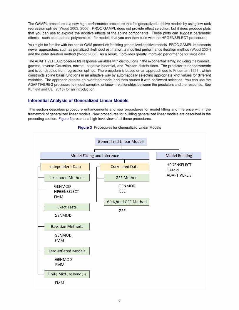
Inferential Analysis of Generalized Linear Models

This section describes procedure enhancements and new procedures for model fitting and inference within theframework of generalized linear models. New procedures for building generalized linear models are described in thepreceding section. Figure 3 presents a high-level view of all these procedures.

Figure 3 Procedures for Generalized Linear Models

6

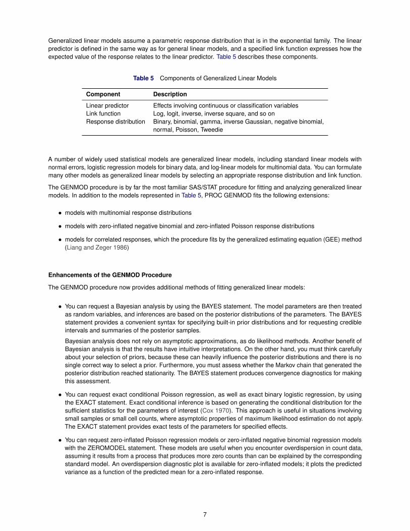
Generalized linear models assume a parametric response distribution that is in the exponential family. The linearpredictor is defined in the same way as for general linear models, and a specified link function expresses how theexpected value of the response relates to the linear predictor. Table 5 describes these components.

Table 5 Components of Generalized Linear Models

Component Description

Linear predictor Effects involving continuous or classification variablesLink function Log, logit, inverse, inverse square, and so onResponse distribution Binary, binomial, gamma, inverse Gaussian, negative binomial,

normal, Poisson, Tweedie

A number of widely used statistical models are generalized linear models, including standard linear models withnormal errors, logistic regression models for binary data, and log-linear models for multinomial data. You can formulatemany other models as generalized linear models by selecting an appropriate response distribution and link function.

The GENMOD procedure is by far the most familiar SAS/STAT procedure for fitting and analyzing generalized linearmodels. In addition to the models represented in Table 5, PROC GENMOD fits the following extensions:

� models with multinomial response distributions

� models with zero-inflated negative binomial and zero-inflated Poisson response distributions

� models for correlated responses, which the procedure fits by the generalized estimating equation (GEE) method(Liang and Zeger 1986)

Enhancements of the GENMOD Procedure

The GENMOD procedure now provides additional methods of fitting generalized linear models:

� You can request a Bayesian analysis by using the BAYES statement. The model parameters are then treatedas random variables, and inferences are based on the posterior distributions of the parameters. The BAYESstatement provides a convenient syntax for specifying built-in prior distributions and for requesting credibleintervals and summaries of the posterior samples.

Bayesian analysis does not rely on asymptotic approximations, as do likelihood methods. Another benefit ofBayesian analysis is that the results have intuitive interpretations. On the other hand, you must think carefullyabout your selection of priors, because these can heavily influence the posterior distributions and there is nosingle correct way to select a prior. Furthermore, you must assess whether the Markov chain that generated theposterior distribution reached stationarity. The BAYES statement produces convergence diagnostics for makingthis assessment.

� You can request exact conditional Poisson regression, as well as exact binary logistic regression, by usingthe EXACT statement. Exact conditional inference is based on generating the conditional distribution for thesufficient statistics for the parameters of interest (Cox 1970). This approach is useful in situations involvingsmall samples or small cell counts, where asymptotic properties of maximum likelihood estimation do not apply.The EXACT statement provides exact tests of the parameters for specified effects.

� You can request zero-inflated Poisson regression models or zero-inflated negative binomial regression modelswith the ZEROMODEL statement. These models are useful when you encounter overdispersion in count data,assuming it results from a process that produces more zero counts than can be explained by the correspondingstandard model. An overdispersion diagnostic plot is available for zero-inflated models; it plots the predictedvariance as a function of the predicted mean for a zero-inflated response.

7

Finite Mixture Models

The FMM procedure fits mixtures of generalized linear models by both maximum likelihood and Bayesian techniques,and it models the effects of covariates on both the component distributions and the mixing probabilities. Finite mixturemodels enable you to account for heterogeneity and overdispersion in your data with a flexible representation thatdescribes the data distribution as a mixture of known distributions.

The FMM procedure provides CLASS and MODEL statements that are familiar from other procedures such as theGLM and GENMOD procedures, and it provides a BAYES statement for requesting built-in Bayesian analysis. TheFMM procedure offers a broad selection of distribution functions and automated model selection methods. Kesslerand McDowell (2012) provide an introduction to the FMM procedure.

Weighted Methods of Analyzing Missing Data in Longitudinal Studies

Studies of longitudinal data are prevalent in fields such as public health, medical research, and social science. Multiplemeasurements are taken on the same subject over time in order to discover changes in the response over time andthe relationship of changes to covariates (Fitzmaurice, Laird, and Ware 2011). Marginal models are used whenpopulation-averaged effects are of interest, and the regression parameters are commonly estimated by the GEEmethod, which is implemented in the GENMOD procedure.

Missing observations caused by dropouts are a particular concern in longitudinal studies. When the analysis isrestricted to complete cases and missingness of responses depends on previous responses, the standard GEEapproach can produce biased parameter estimates. The GEE procedure implements inverse probability-weightedGEE methods that account for dropouts under the assumption that data are missing at random (MAR); see Robinsand Rotnitzky (1995) and Preisser, Lohman, and Rathouz (2002). These methods can produce unbiased estimates.

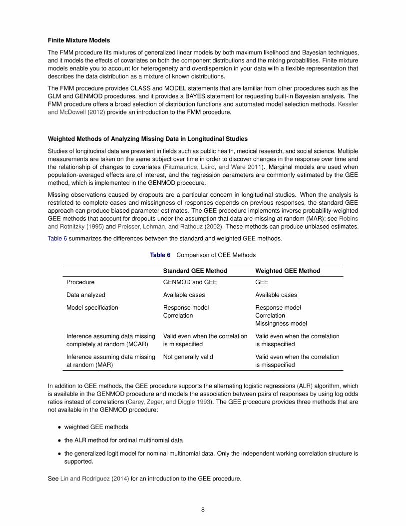
Table 6 summarizes the differences between the standard and weighted GEE methods.

Table 6 Comparison of GEE Methods

Standard GEE Method Weighted GEE Method

Procedure GENMOD and GEE GEE

Data analyzed Available cases Available cases

Model specification Response model Response modelCorrelation Correlation

Missingness model

Inference assuming data missing Valid even when the correlation Valid even when the correlationcompletely at random (MCAR) is misspecified is misspecified

Inference assuming data missing Not generally valid Valid even when the correlationat random (MAR) is misspecified

In addition to GEE methods, the GEE procedure supports the alternating logistic regressions (ALR) algorithm, whichis available in the GENMOD procedure and models the association between pairs of responses by using log oddsratios instead of correlations (Carey, Zeger, and Diggle 1993). The GEE procedure provides three methods that arenot available in the GENMOD procedure:

� weighted GEE methods

� the ALR method for ordinal multinomial data

� the generalized logit model for nominal multinomial data. Only the independent working correlation structure issupported.

See Lin and Rodriguez (2014) for an introduction to the GEE procedure.

8

Survival Analysis

Survival analysis deals with time-to-event data that are incomplete due to censoring or competing risks:

� Observations are right-censored when the only information at a given time is that the event of interest has notyet occurred. Likewise, observations are left-censored when the only information at a given time is that theevent has already occurred. Observations are interval-censored when the only information is that the event hasoccurred within a known interval.

� Competing risks are events that impede the observation of the event of interest or that modify the probabilitythat this event will occur. For example, in cardiovascular studies, deaths from other causes such as cancer areconsidered competing risks.

SAS/STAT software provides specialized procedures for performing survival analysis for right-censored data. Threeof these, the LIFETEST, LIFEREG, and PHREG procedures, are particularly well known because they have beenavailable for many years.

The LIFETEST procedure specializes in estimation and hypothesis testing; it computes the Kaplan-Meier estimate ofa survivor function and provides the log-rank test for comparing survival curves between groups of observations. TheLIFEREG and PHREG procedures specialize in modeling the outcome of interest, but with a clear distinction: PROCLIFEREG fits parametric accelerated failure time (AFT) models, while PROC PHREG fits semiparametric regressionmodels, including the Cox proportional hazards model.

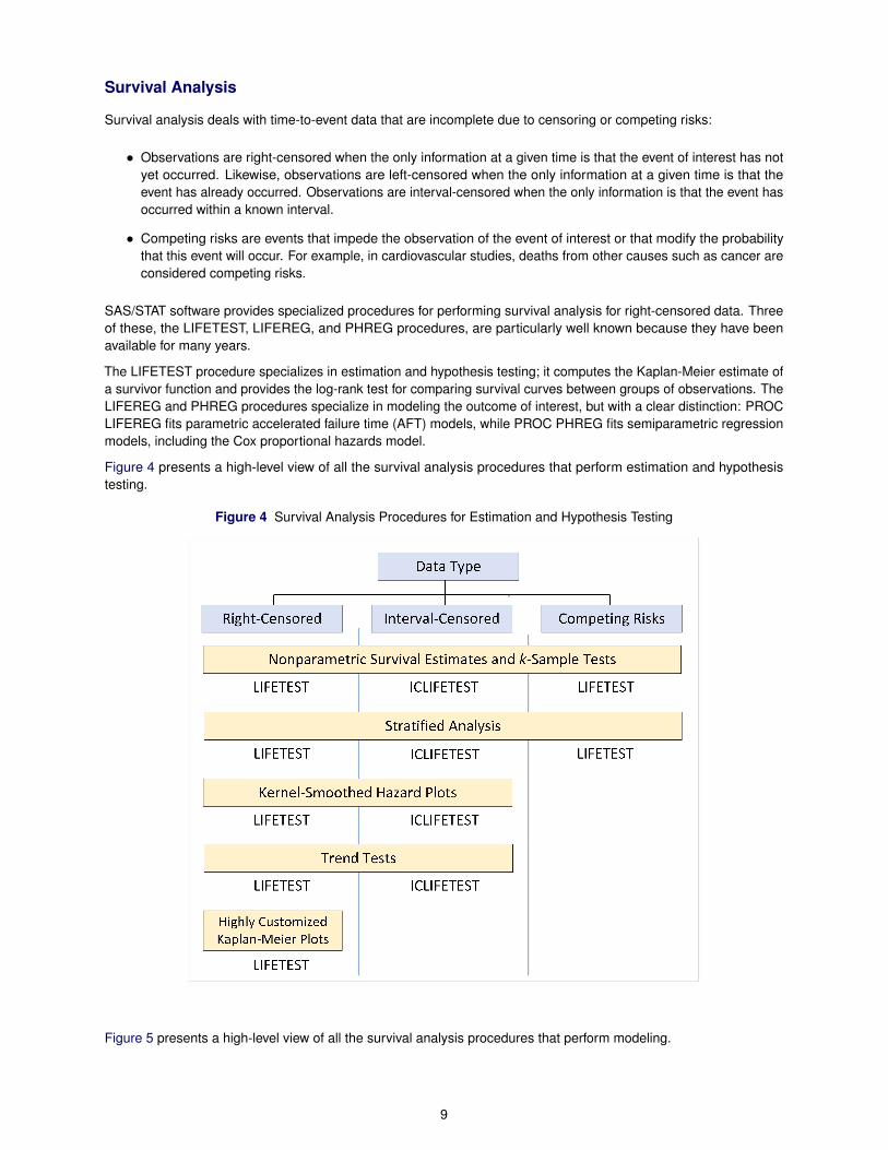
Figure 4 presents a high-level view of all the survival analysis procedures that perform estimation and hypothesistesting.

Figure 4 Survival Analysis Procedures for Estimation and Hypothesis Testing

Figure 5 presents a high-level view of all the survival analysis procedures that perform modeling.

9

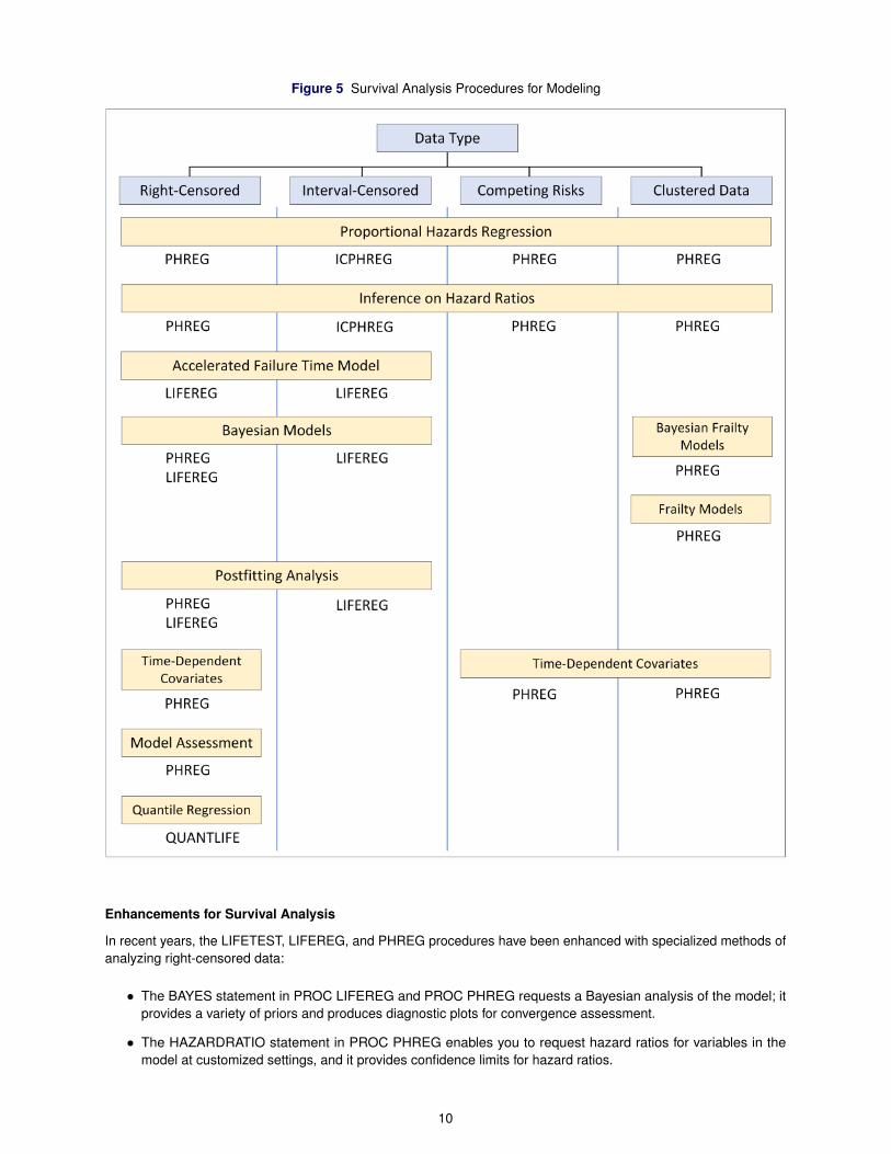
Figure 5 Survival Analysis Procedures for Modeling

Enhancements for Survival Analysis

In recent years, the LIFETEST, LIFEREG, and PHREG procedures have been enhanced with specialized methods ofanalyzing right-censored data:

� The BAYES statement in PROC LIFEREG and PROC PHREG requests a Bayesian analysis of the model; itprovides a variety of priors and produces diagnostic plots for convergence assessment.

� The HAZARDRATIO statement in PROC PHREG enables you to request hazard ratios for variables in themodel at customized settings, and it provides confidence limits for hazard ratios.

10

� The PHREG procedure provides methods of model assessment, including the Schemper-Henderson statistic,two versions of concordance statistics, and time-dependent receiver-operator characteristic (ROC) curves.

� The Kaplan-Meier plot that is produced by PROC LIFETEST is now highly customizable through the use ofprocedure options, graph template modifications, and style template modifications. Kuhfeld and So (2013)provide examples of these approaches.

The survival analysis capabilities of SAS/STAT have also been extended to handle types of time-to-event data otherthan right-censored data:

� Two new procedures, PROC ICLIFETEST and PROC ICPHREG, specialize in the analysis of interval-censoreddata and serve as counterparts of PROC LIFETEST and PROC PHREG.

� The LIFETEST and PHREG procedures have been enhanced with specialized methods that analyze thecumulative incidence function (CIF) for competing risks data.

� The RANDOM statement in PHREG provides facilities for fitting frailty models, which handle correlationsbetween failures in clustered data.

Another new procedure, the QUANTLIFE procedure, uses quantile regression to analyze survival data and isparticularly useful for modeling heterogeneous data.

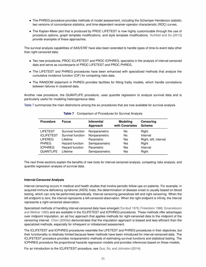
Table 7 summarizes the main distinctions among the six procedures that are now available for survival analysis.

Table 7 Comparison of Procedures for Survival Analysis

Procedure Focus Inferential Modeling CensoringApproach with Covariates Scheme

LIFETEST Survival function Nonparametric No RightICLIFETEST Survival function Nonparametric No IntervalLIFEREG Lifetime Parametric Yes Right, left, intervalPHREG Hazard function Semiparametric Yes RightICPHREG Hazard function Parametric Yes IntervalQUANTLIFE Lifetime Semiparametric Yes Right

The next three sections explain the benefits of new tools for interval-censored analysis, competing risks analysis, andquantile regression analysis of survival data.

Interval-Censored Analysis

Interval censoring occurs in medical and health studies that involve periodic follow-ups on patients. For example, inacquired immune deficiency syndrome (AIDS) trials, the determination of disease onset is usually based on bloodtesting, which can only be performed periodically. Interval censoring generalizes left and right censoring. When theleft endpoint is zero, the interval represents a left-censored observation. When the right endpoint is infinity, the intervalrepresents a right-censored observation.

Specialized methods of handling interval-censored data have emerged (Turnbull 1976; Finkelstein 1986; Groeneboomand Wellner 1992) and are available in the ICLIFETEST and ICPHREG procedures. These methods offer advantagesover midpoint imputation, an ad hoc approach that applies methods for right-censored data to the midpoint of thecensoring interval. Chen (2009a) demonstrates that the imputation approach is biased and less efficient than thespecialized methods, especially for infrequent or imbalanced assessment.

The ICLIFETEST and ICPHREG procedures resemble the LIFETEST and PHREG procedures in their objectives, buttheir functionality is relatively limited because fewer methods have been introduced for interval-censored data. TheICLIFETEST procedure provides nonparametric methods of estimating survival functions and statistical testing. TheICPHREG procedure fits proportional hazards regression models and provides inferences based on these models.

For an introduction to the ICLIFETEST procedure, see Guo, So, and Johnston (2014).

11

Analysis of Competing Risks

Recent enhancements of the LIFETEST and PHREG procedures provide state-of-the-art techniques for the analysisof right-censored data with competing risks. You can use the LIFETEST procedure to perform nonparametric analysesand the PHREG procedure to perform regression analyses.

The concepts of a survival function and a hazard function, which form the basis for standard survival analysis, areinadequate for studying competing risks because once a subject experiences an event other than the event of interest,information about the latter can no longer be ascertained reliably. Instead, the analysis of competing risks is based onthe analogous concepts of a cumulative incidence function (CIF) and a cause-specific hazard (CSH) function. TheCIF, which is defined as the probability subdistribution function of failure from a specific cause, characterizes theoccurrence of a cause-specific outcome over time. The CSH function measures the instantaneous rate of failing froma specific cause in the presence of other causes.

By treating observations of other types of events as censored observations of the event of interest, you can analyze theCSH function for the cause of interest by using certain standard methods, such as the log-rank test in the LIFETESTprocedure and Cox regression in the PHREG procedure. However, to analyze the CIF, you need specialized methods,such as those recently provided in the LIFETEST procedure and the PHREG procedure.

The model of Fine and Gray (1999), implemented in the PHREG procedure, extends the Cox model to the CIFsetting. The test due to Gray (1988) serves as a counterpart of the log-rank test for testing the equality of CIFs,and is available in the LIFETEST procedure along with a nonparametric estimator of the CIF. You can request CIFanalyses in the LIFETEST and PHREG procedures by specifying the code that represents the cause of interest withthe EVENTCODE= option. So, Lin, and Johnston (2015) explain how to perform competing risks regression by usingthe PHREG procedure.

Survival Analysis Based on Quantile Regression

The quantile regression approach to survival analysis, now available in the QUANTLIFE procedure, is useful whenyou are modeling the survival time and the effects of covariates on the lifetime distribution differ with the covariates.You can use PROC QUANTLIFE to explore such effects—for example, when the variation in the lifetime increaseswith a continuous covariate.

To decide when to use the QUANTLIFE procedure, you should understand how the quantile regression approachcompares with standard methods available in the LIFETEST, LIFEREG, and PHREG procedures. Each method hasits advantages and limitations.

Quantile regression is a distribution-free approach in the sense that inference about the regression parameters for aparticular quantile of the lifetime depends only on the conditional distribution near that quantile. By comparison, theAFT model in the LIFEREG procedure is more restrictive in its parametric assumption.

Both the Cox proportional model in the PHREG procedure and the AFT model involve an iid error assumption under asuitable transformation of the survival time (Koenker and Geling 2001). This means that covariate effects can shift thelocation but not the shape of the conditional density for the transformed lifetime. The additional flexibility of quantileregression for modeling the shape can be important when, for example, you are concerned about treatment effects onlonger lifetimes.

The QUANTLIFE and LIFEREG procedures both use a regression method to model the lifetime. The LIFEREGprocedure provides an efficient estimator for the regression parameters if you are willing to assume a parametricdistribution for the lifetime. The regression coefficients computed by the LIFEREG procedure are interpreted as theeffect on the mean of the lifetime, and the regression coefficients computed by the QUANTLIFE procedure apply tospecified quantiles of the lifetime.

Unlike the QUANTLIFE procedure, the PHREG procedure models the hazard function. Both of these procedures aresemiparametric, but in different ways. The Cox model requires no parametric assumption about the baseline hazardfunction. Another advantage of the Cox model is that it can incorporate time-dependent covariates.

Lin and Rodriguez (2013) provide an introduction to the QUANTLIFE procedure.

12

Analysis of Mixed Models

When you fit statistical models to data, it is common to assume that all the observations are uncorrelated. Thestandard linear model procedures—GLM, REG, GLMSELECT, and HPREG—all make this assumption. But when thatassumption is violated, it can have a huge impact on the validity of the inferences that you make, and that is when youneed mixed models. Mixed models incorporate both fixed effects, which affect only the mean of the response, andrandom effects, which relate to the covariance between observations.

The MIXED procedure is the flagship SAS/STAT procedure for dealing with linear mixed models. PROC MIXEDextends the versatile features for specifying fixed effects in linear models that you find in many SAS/STAT procedureswith similarly versatile features for specifying how random effects induce correlation. Likewise, PROC MIXED extendsthe inferential tools for linear models with fixed effects—for example, Type 3 tests, tests for linear contrasts, andLS-means—with tests and methods that are appropriate for correlation structures.

Although PROC MIXED provides the generality that you need for model estimation and postfit inference, it is notcomputationally efficient for certain important special cases, including the following:

� linear mixed models with thousands of levels for the fixed and/or random effects

� linear mixed models with hierarchically nested fixed and/or random effects, possibly with hundreds or thousandsof levels at each stage of the hierarchy

For these models, which are large and sparse, you need specialized methods. The HPMIXED procedure implementsthese methods by taking advantage of sparse matrix techniques. PROC HPMIXED does sacrifice certain inferentialtools that are available in PROC MIXED but cannot be implemented sparsely. However, if your mixed models fallinto these special categories, PROC HPMIXED can often run much faster than PROC MIXED. Wang and Tobias(2009) and Kiernan, Tao, and Gibbs (2016) describe situations that call for the methods in PROC HPMIXED, and theydiscuss the substantial gains in performance that it provides.

Both the MIXED and HPMIXED procedures deal with responses and random effects that are assumed to be normallydistributed. If your response has a nonnormal distribution that belongs to the exponential family—for example, if it hasa binary logistic or Poisson distribution—then you need the GLIMMIX procedure, which fits generalized linear mixedmodels. PROC GLIMMIX can use pseudo-likelihood or marginal maximum likelihood estimation to fit mixed modelswith a variety of nonnormal error distributions. Schabenberger (2005) outlines the capabilities of PROC GLIMMIX andprovides examples that demonstrate its great flexibility for modeling correlated data.

If you need to fit linear mixed models, then one of the three procedures discussed so far in this section—MIXED,HPMIXED, and GLIMMIX—is what you need. But what if you need to fit a random coefficients model in which thecoefficients enter the model nonlinearly? Or what if you are fitting a nonlinear mixed model for a pharmacokineticapplication where the likelihood depends on solving a system of differential equations? The NLMIXED procedure canfit such models; it enables you to specify a distribution for the response, conditional on the random effects, that hasa standard form—such as normal, binary, or Poisson—or a general form that you express with SAS programmingstatements.

Although both PROC GLIMMIX and PROC NLMIXED enable you to fit models for nonnormal responses, the estimationmethods they use require the random effects to be normally distributed. If you need to fit models with nonnormalrandom effects, then you need to move beyond likelihood methods and consider Bayesian methods, for which theMCMC procedure is the most versatile procedure in SAS/STAT.

Instead of maximizing a likelihood, the Bayesian approach treats all unknown quantities in a model, including both thefixed and random effects, as random variables. The objective is to estimate the joint posterior distribution, often byusing the Markov chain Monte Carlo approach (Gelfand et al. 1990). The marginal distribution of the fixed-effectsparameters is obtained by using a numerical Monte Carlo method that is based on the Markov chain samples.

In PROC MCMC, you specify the details of a Bayesian model with a combination of procedure statements (such asthe PARMS, PRIOR, MODEL, and RANDOM statements) and SAS programming statements. Like the NLMIXEDprocedure, the MCMC procedure does not assume linearity and it handles a wide range of models. The complexBayesian models that you can fit with PROC MCMC include linear, generalized linear, and nonlinear random-effectsmodels.

The tutorial papers by Chen (2009b, 2011, 2013) introduce the MCMC procedure. Chen, Brown, and Stokes (2016)offer guidance on using PROC MCMC to perform Bayesian analysis of models for which PROC MIXED and PROC

13

GLIMMIX implement likelihood methods. Chen and Stokes (2017) illustrate the use of PROC MCMC to fit variousmultilevel hierarchical models that incorporate complex structures and data dependencies.

In principle, the MCMC procedure is the most general SAS/STAT procedure for analyzing mixed models. It can handlenormal data and linear models (like the MIXED procedure), nonnormal data and generalized linear models (like theGLIMMIX, GENMOD, and GEE procedures), and nonlinear models (like the NLMIXED procedure). In addition, theMCMC procedure can handle nonnormal random effects, multilevel random effects, and missing data in ways thatare not available with the other procedures. Of course, with this generality you give up much of the convenience andspecific analytic features of the more specialized procedures. Thus, the MIXED, HPMIXED, GLIMMIX, and NLMIXEDprocedures should be your go-to tools for most practical applications of mixed models. The MCMC procedure shouldbe in your toolbox for applications that the other procedures cannot handle, and for situations in which Bayesianmodeling is appropriate.

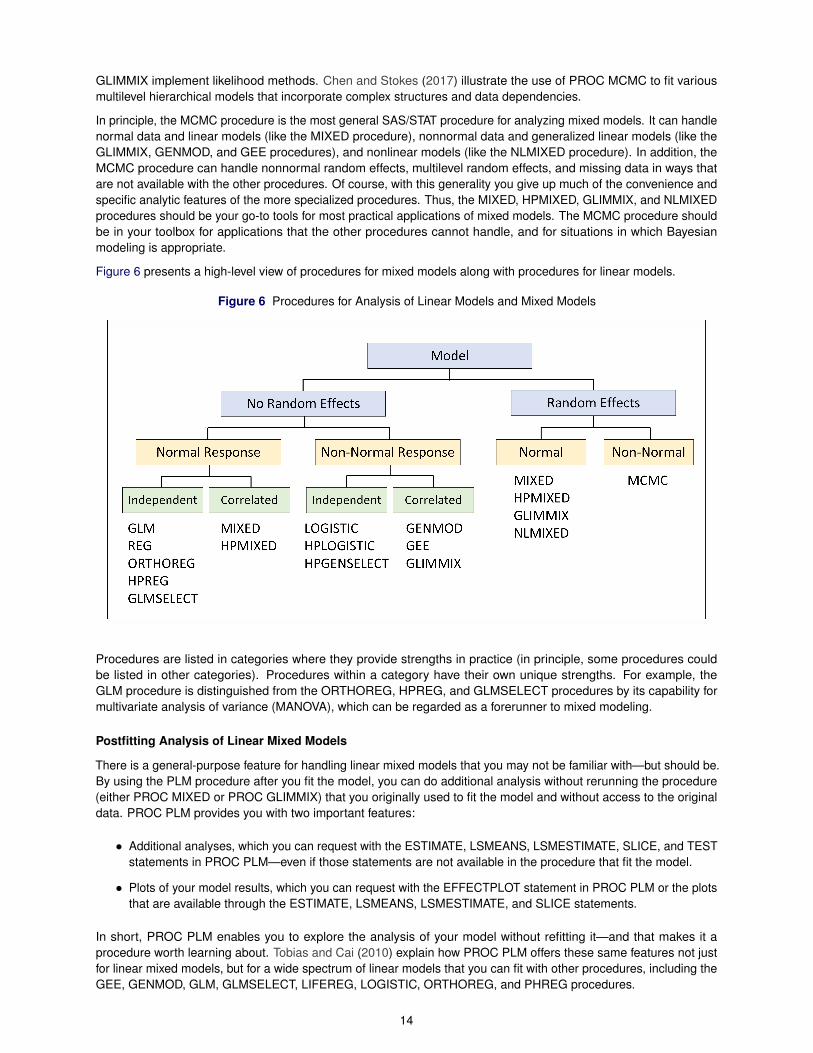
Figure 6 presents a high-level view of procedures for mixed models along with procedures for linear models.

Figure 6 Procedures for Analysis of Linear Models and Mixed Models

Procedures are listed in categories where they provide strengths in practice (in principle, some procedures couldbe listed in other categories). Procedures within a category have their own unique strengths. For example, theGLM procedure is distinguished from the ORTHOREG, HPREG, and GLMSELECT procedures by its capability formultivariate analysis of variance (MANOVA), which can be regarded as a forerunner to mixed modeling.

Postfitting Analysis of Linear Mixed Models

There is a general-purpose feature for handling linear mixed models that you may not be familiar with—but should be.By using the PLM procedure after you fit the model, you can do additional analysis without rerunning the procedure(either PROC MIXED or PROC GLIMMIX) that you originally used to fit the model and without access to the originaldata. PROC PLM provides you with two important features:

� Additional analyses, which you can request with the ESTIMATE, LSMEANS, LSMESTIMATE, SLICE, and TESTstatements in PROC PLM—even if those statements are not available in the procedure that fit the model.

� Plots of your model results, which you can request with the EFFECTPLOT statement in PROC PLM or the plotsthat are available through the ESTIMATE, LSMEANS, LSMESTIMATE, and SLICE statements.

In short, PROC PLM enables you to explore the analysis of your model without refitting it—and that makes it aprocedure worth learning about. Tobias and Cai (2010) explain how PROC PLM offers these same features not justfor linear mixed models, but for a wide spectrum of linear models that you can fit with other procedures, including theGEE, GENMOD, GLM, GLMSELECT, LIFEREG, LOGISTIC, ORTHOREG, and PHREG procedures.

14

Summary

This paper describes important new tools that SAS/STAT has added in four areas:

� Regression model building� Inferential analysis of generalized linear models� Survival analysis� Analysis of mixed models

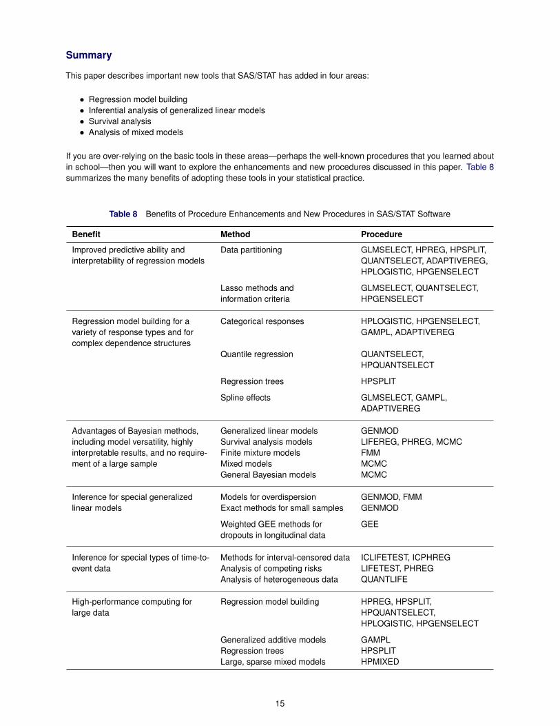
If you are over-relying on the basic tools in these areas—perhaps the well-known procedures that you learned aboutin school—then you will want to explore the enhancements and new procedures discussed in this paper. Table 8summarizes the many benefits of adopting these tools in your statistical practice.

Table 8 Benefits of Procedure Enhancements and New Procedures in SAS/STAT Software

Benefit Method Procedure

Improved predictive ability and Data partitioning GLMSELECT, HPREG, HPSPLIT,interpretability of regression models QUANTSELECT, ADAPTIVEREG,

HPLOGISTIC, HPGENSELECT

Lasso methods and GLMSELECT, QUANTSELECT,information criteria HPGENSELECT

Regression model building for a Categorical responses HPLOGISTIC, HPGENSELECT,variety of response types and for GAMPL, ADAPTIVEREGcomplex dependence structures

Quantile regression QUANTSELECT,HPQUANTSELECT

Regression trees HPSPLIT

Spline effects GLMSELECT, GAMPL,ADAPTIVEREG

Advantages of Bayesian methods, Generalized linear models GENMODincluding model versatility, highly Survival analysis models LIFEREG, PHREG, MCMCinterpretable results, and no require- Finite mixture models FMMment of a large sample Mixed models MCMC

General Bayesian models MCMC

Inference for special generalized Models for overdispersion GENMOD, FMMlinear models Exact methods for small samples GENMOD

Weighted GEE methods for GEEdropouts in longitudinal data

Inference for special types of time-to- Methods for interval-censored data ICLIFETEST, ICPHREGevent data Analysis of competing risks LIFETEST, PHREG

Analysis of heterogeneous data QUANTLIFE

High-performance computing for Regression model building HPREG, HPSPLIT,large data HPQUANTSELECT,

HPLOGISTIC, HPGENSELECT

Generalized additive models GAMPLRegression trees HPSPLITLarge, sparse mixed models HPMIXED

15

Keeping Up with New Releases of SAS/STAT

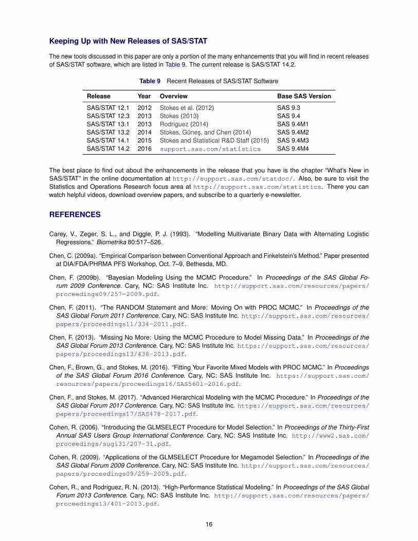
The new tools discussed in this paper are only a portion of the many enhancements that you will find in recent releasesof SAS/STAT software, which are listed in Table 9. The current release is SAS/STAT 14.2.

Table 9 Recent Releases of SAS/STAT Software

Release Year Overview Base SAS Version

SAS/STAT 12.1 2012 Stokes et al. (2012) SAS 9.3SAS/STAT 12.3 2013 Stokes (2013) SAS 9.4SAS/STAT 13.1 2013 Rodriguez (2014) SAS 9.4M1SAS/STAT 13.2 2014 Stokes, Günes, and Chen (2014) SAS 9.4M2SAS/STAT 14.1 2015 Stokes and Statistical R&D Staff (2015) SAS 9.4M3SAS/STAT 14.2 2016 support.sas.com/statistics SAS 9.4M4

The best place to find out about the enhancements in the release that you have is the chapter “What’s New inSAS/STAT” in the online documentation at http://support.sas.com/statdoc/. Also, be sure to visit theStatistics and Operations Research focus area at http://support.sas.com/statistics. There you canwatch helpful videos, download overview papers, and subscribe to a quarterly e-newsletter.

REFERENCES

Carey, V., Zeger, S. L., and Diggle, P. J. (1993). “Modelling Multivariate Binary Data with Alternating LogisticRegressions.” Biometrika 80:517–526.

Chen, C. (2009a). “Empirical Comparison between Conventional Approach and Finkelstein’s Method.” Paper presentedat DIA/FDA/PHRMA PFS Workshop, Oct. 7–9, Bethesda, MD.

Chen, F. (2009b). “Bayesian Modeling Using the MCMC Procedure.” In Proceedings of the SAS Global Fo-rum 2009 Conference. Cary, NC: SAS Institute Inc. http://support.sas.com/resources/papers/proceedings09/257-2009.pdf.

Chen, F. (2011). “The RANDOM Statement and More: Moving On with PROC MCMC.” In Proceedings of theSAS Global Forum 2011 Conference. Cary, NC: SAS Institute Inc. http://support.sas.com/resources/papers/proceedings11/334-2011.pdf.

Chen, F. (2013). “Missing No More: Using the MCMC Procedure to Model Missing Data.” In Proceedings of theSAS Global Forum 2013 Conference. Cary, NC: SAS Institute Inc. https://support.sas.com/resources/papers/proceedings13/436-2013.pdf.

Chen, F., Brown, G., and Stokes, M. (2016). “Fitting Your Favorite Mixed Models with PROC MCMC.” In Proceedingsof the SAS Global Forum 2016 Conference. Cary, NC: SAS Institute Inc. https://support.sas.com/resources/papers/proceedings16/SAS5601-2016.pdf.

Chen, F., and Stokes, M. (2017). “Advanced Hierarchical Modeling with the MCMC Procedure.” In Proceedings of theSAS Global Forum 2017 Conference. Cary, NC: SAS Institute Inc. https://support.sas.com/resources/papers/proceedings17/SAS478-2017.pdf.

Cohen, R. (2006). “Introducing the GLMSELECT Procedure for Model Selection.” In Proceedings of the Thirty-FirstAnnual SAS Users Group International Conference. Cary, NC: SAS Institute Inc. http://www2.sas.com/proceedings/sugi31/207-31.pdf.

Cohen, R. (2009). “Applications of the GLMSELECT Procedure for Megamodel Selection.” In Proceedings of theSAS Global Forum 2009 Conference. Cary, NC: SAS Institute Inc. http://support.sas.com/resources/papers/proceedings09/259-2009.pdf.

Cohen, R., and Rodriguez, R. N. (2013). “High-Performance Statistical Modeling.” In Proceedings of the SAS GlobalForum 2013 Conference. Cary, NC: SAS Institute Inc. http://support.sas.com/resources/papers/proceedings13/401-2013.pdf.

16

Cox, D. R. (1970). Analysis of Binary Data. London: Metheun.

Fine, J. P., and Gray, R. J. (1999). “A Proportional Hazards Model for the Subdistribution of a Competing Risk.” Journalof the American Statistical Association 94:496–509.

Finkelstein, D. M. (1986). “A Proportional Hazards Model for Interval-Censored Failure Time Data.” Biometrics42:845–854.

Fitzmaurice, G. M., Laird, N. M., and Ware, J. H. (2011). Applied Longitudinal Analysis. 2nd ed. Hoboken, NJ: JohnWiley & Sons.

Friedman, J. H. (1991). “Multivariate Adaptive Regression Splines.” Annals of Statistics 19:1–67.

Gelfand, A. E., Hills, S. E., Racine-Poon, A., and Smith, A. F. M. (1990). “Illustration of Bayesian Inference in NormalData Models Using Gibbs Sampling.” Journal of the American Statistical Association 85:972–985.

Gibbs, P., Tobias, R., Kiernan, K., and Tao, J. (2013). “Having an EFFECT: More General Linear Modeling and Analysiswith the New EFFECT Statement in SAS/STAT Software.” In Proceedings of the SAS Global Forum 2013 Conference.Cary, NC: SAS Institute Inc. https://support.sas.com/resources/papers/proceedings13/437-2013.pdf.

Gray, R. J. (1988). “A Class of K-Sample Tests for Comparing the Cumulative Incidence of a Competing Risk.” Annalsof Statistics 16:1141–1154.

Groeneboom, P., and Wellner, J. A. (1992). Information Bounds and Nonparametric Maximum Likelihood Estimation.Basel: Birkhäuser.

Günes, F. (2015). “Penalized Regression Methods for Linear Models in SAS/STAT.” In Proceedings of the SAS GlobalForum 2015 Conference. Cary, NC: SAS Institute Inc. http://support.sas.com/rnd/app/stat/papers/2015/PenalizedRegression_LinearModels.pdf.

Guo, C., So, Y., and Johnston, G. (2014). “Analyzing Interval-Censored Data with the ICLIFETEST Procedure.” InProceedings of the SAS Global Forum 2014 Conference. Cary, NC: SAS Institute Inc. http://support.sas.com/resources/papers/proceedings14/SAS279-2014.pdf.

Hastie, T., Tibshirani, R., and Wainwright, M. (2015). Statistical Learning with Sparsity: The Lasso and Generalizations.Boca Raton, FL: CRC Press.

Johnston, G., and Rodriguez, R. N. (2015). “Introducing the HPGENSELECT Procedure: Model Selection forGeneralized Linear Models and More.” In Proceedings of the SAS Global Forum 2015 Conference. Cary, NC: SASInstitute Inc. http://support.sas.com/resources/papers/proceedings15/SAS1742-2015.pdf.

Kessler, D., and McDowell, A. (2012). “Introducing the FMM Procedure for Finite Mixture Models.” In Proceedings of theSAS Global Forum 2012 Conference. Cary, NC: SAS Institute Inc. http://support.sas.com/resources/papers/proceedings12/328-2012.pdf.

Kiernan, K., Tao, J., and Gibbs, P. (2016). “Tips and Strategies for Mixed Modeling with SAS/STAT Procedures.” InProceedings of the SAS Global Forum 2016 Conference. Cary, NC: SAS Institute Inc. http://support.sas.com/resources/papers/proceedings16/SAS6403-2016.pdf.

Koenker, R., and Bassett, G. W. (1978). “Regression Quantiles.” Econometrica 46:33–50.

Koenker, R., and Geling, O. (2001). “Reappraising Medfly Longevity: A Quantile Regression Survival Analysis.”Journal of the American Statistical Association 96:458–468.

Kuhfeld, W., and Cai, W. (2013). “Introducing the New ADAPTIVEREG Procedure for Adaptive Regression.” InProceedings of the SAS Global Forum 2013 Conference. Cary, NC: SAS Institute Inc. https://support.sas.com/resources/papers/proceedings13/457-2013.pdf.

Kuhfeld, W. F., and So, Y. (2013). “Creating and Customizing the Kaplan-Meier Survival Plot in PROC LIFETEST.” InProceedings of the SAS Global Forum 2013 Conference. Cary, NC: SAS Institute Inc. https://support.sas.com/resources/papers/proceedings13/427-2013.pdf.

Liang, K.-Y., and Zeger, S. L. (1986). “Longitudinal Data Analysis Using Generalized Linear Models.” Biometrika73:13–22.

17

Lin, G., and Rodriguez, R. N. (2013). “Using the QUANTLIFE Procedure for Survival Analysis.” In Proceedings of theSAS Global Forum 2013 Conference. Cary, NC: SAS Institute Inc. https://support.sas.com/resources/papers/proceedings13/421-2013.pdf.

Lin, G., and Rodriguez, R. N. (2014). “Weighted Methods for Analyzing Missing Data with the GEE Procedure.” InProceedings of the SAS Global Forum 2014 Conference. Cary, NC: SAS Institute Inc. http://support.sas.com/resources/papers/proceedings14/SAS166-2014.pdf.

Preisser, J. S., Lohman, K. K., and Rathouz, P. J. (2002). “Performance of Weighted Estimating Equations forLongitudinal Binary Data with Drop-Outs Missing at Random.” Statistics in Medicine 21:3035–3054.

Robins, J. M., and Rotnitzky, A. (1995). “Semiparametric Efficiency in Multivariate Regression Models with MissingData.” Journal of the American Statistical Association 90:122–129.

Rodriguez, R. N. (2014). “SAS/STAT 13.1: Round-Up.” In Proceedings of the SAS Global Forum 2014 Conference.Cary, NC: SAS Institute Inc. http://support.sas.com/resources/papers/proceedings14/SAS181-2014.pdf.

Rodriguez, R. N., and Yao, Y. (2017). “Five Things You Should Know about Quantile Regression.” In Proceedings of theSAS Global Forum 2017 Conference. Cary, NC: SAS Institute Inc. http://support.sas.com/resources/papers/proceedings17/SAS525-2017.pdf.

Schabenberger, O. (2005). “Introducing the GLIMMIX Procedure for Generalized Linear Mixed Models.” In Proceedingsof the Thirtieth Annual SAS Users Group International Conference. Cary, NC: SAS Institute Inc. http://www2.sas.com/proceedings/sugi30/196-30.pdf.

So, Y., Lin, G., and Johnston, G. (2015). “Using the PHREG Procedure to Analyze Competing-Risks Data.” InProceedings of the SAS Global Forum 2015 Conference. Cary, NC: SAS Institute Inc. http://support.sas.com/resources/papers/proceedings15/SAS1855-2015.pdf.

Stokes, M. (2013). “Current Directions in SAS/STAT Software Development.” In Proceedings of the SAS GlobalForum 2013 Conference. Cary, NC: SAS Institute Inc. http://support.sas.com/resources/papers/proceedings13/432-2013.pdf.

Stokes, M., Chen, F., Yuan, Y., and Cai, W. (2012). “Look Out: After SAS/STAT 9.3 Comes SAS/STAT 12.1!” InProceedings of the SAS Global Forum 2012 Conference. Cary, NC: SAS Institute Inc. http://support.sas.com/resources/papers/proceedings12/313-2012.pdf.

Stokes, M., Günes, F., and Chen, F. (2014). “An Introduction to Bayesian Analysis with SAS/STAT Software.” InProceedings of the SAS Global Forum 2014 Conference. Cary, NC: SAS Institute Inc. http://support.sas.com/resources/papers/proceedings14/SAS400-2014.pdf.

Stokes, M., and Statistical R&D Staff (2015). “SAS/STAT 14.1: Methods for Massive, Missing, or Multifaceted Data.” InProceedings of the SAS Global Forum 2015 Conference. Cary, NC: SAS Institute Inc. http://support.sas.com/resources/papers/proceedings15/SAS1940-2015.pdf.

Tibshirani, R. (1996). “Regression Shrinkage and Selection via the Lasso.” Journal of the Royal Statistical Society,Series B 58:267–288.

Tobias, R. D., and Cai, W. (2010). “Introducing PROC PLM and Postfitting Analysis for Very General Linear Modelsin SAS/STAT 9.22.” In Proceedings of the SAS Global Forum 2010 Conference. Cary, NC: SAS Institute Inc.http://support.sas.com/resources/papers/proceedings10/258-2010.pdf.

Turnbull, B. W. (1976). “The Empirical Distribution Function with Arbitrarily Grouped, Censored, and Truncated Data.”Journal of the Royal Statistical Society, Series B 38:290–295.

Wang, T., and Tobias, R. D. (2009). “All the Cows in Canada: Massive Mixed Modeling with the HPMIXED Procedurein SAS 9.2.” In Proceedings of the SAS Global Forum 2009 Conference. Cary, NC: SAS Institute Inc. https://support.sas.com/resources/papers/proceedings09/256-2009.pdf.

Wood, S. (2003). “Thin Plate Regression Splines.” Journal of the Royal Statistical Society, Series B 65:95–114.

Wood, S. (2004). “Stable and Efficient Multiple Smoothing Parameter Estimation for Generalized Additive Models.”Journal of the American Statistical Association 99:673–686.

Wood, S. (2006). Generalized Additive Models. Boca Raton, FL: Chapman & Hall/CRC.

18

Acknowledgments

The authors are grateful to Susan Rodriguez for editorial assistance and to Weijie Cai, Fang Chen, Changbin Guo,Michael Lamm, and Maura Stokes for helpful suggestions.

Contact Information

Your comments and questions are valued and encouraged. You can contact the authors at the following addresses:

Robert N. Rodriguez Phil Gibbs Randy TobiasSAS Institute Inc. SAS Institute Inc. SAS Institute Inc.SAS Campus Drive SAS Campus Drive SAS Campus DriveCary, NC 27513 Cary, NC 27513 Cary, NC 27513Bob.Rodriguez@sas.com Phil.Gibbs@sas.com Randy.Tobias@sas.com

SAS and all other SAS Institute Inc. product or service names are registered trademarks or trademarks of SASInstitute Inc. in the USA and other countries. ® indicates USA registration. Other brand and product names aretrademarks of their respective companies.

19