STEM Careers and Technological Change

David J. DemingHarvard University and NBER

Kadeem NorayHarvard University∗

September 2018

Abstract

Science, Technology, Engineering, and Math (STEM) jobs are a key contributor to eco-nomic growth and national competitiveness. Yet STEM workers are perceived to be inshort supply. This paper shows that the “STEM shortage” phenomenon is explainedby technological change, which introduces new job tasks and makes old ones obsolete.We find that the initially high economic return to applied STEM degrees declines bymore than 50 percent in the first decade of working life. This coincides with a rapidexit of college graduates from STEM occupations. Using detailed job vacancy data,we show that STEM jobs changed especially quickly over the last decade, leading toflatter age-earnings profiles as the skills of older cohorts became obsolete. Our findingshighlight the importance of technology-specific skills in explaining life-cycle returns toeducation, and show that STEM jobs are the leading edge of technology diffusion inthe labor market.

∗Emails: david_deming@harvard.edu; knoray@g.harvard.edu. Thanks to seminar participants at George-town University and Harvard University for helpful comments. We also thank Bledi Taska and the staff atBurning Glass Technologies for generously sharing their data, and Suchi Akmanchi for excellent researchassistance. All errors are our own.

1 Introduction

Science, Technology, Engineering, and Math (STEM) jobs are a key contributor to innova-

tion and productivity growth in most advanced economies (e.g. Griliches 1992, Jones 1995,

Carnevale et al. 2011, Peri et al. 2015). Despite the high labor market payoff for college

students majoring in STEM fields, there is a widespread perception that STEM workers are

in short supply (Arcidiacono 2004, Carnevale et al. 2012, Kinsler and Pavan 2015, Cappelli

2015, Arcidiacono et al. 2016). Yet STEM employment in the U.S. has grown slowly in the

past two decades, and 58 percent of STEM graduates leave the field within 10 years after

receiving their degree (Carnevale et al. 2011, Charette 2013, Deming 2017).

In this paper we argue that perceived skill shortages, high initial returns for STEMmajors

and exit from STEM careers over time have a common cause - technological change, which

introduces new job tasks and makes old tasks obsolete (e.g. Rosen 1975). STEM graduates

in applied subjects such as engineering and computer science earn higher wages initially,

because they learn job-relevant skills in school. Yet over time, new technologies replace the

skills and tasks originally learned by older graduates, causing them to experience flatter

wage growth and eventually exit the STEM workforce. Faster technological progress creates

a greater sense of shortage, but it is the new STEM skills that are scarce, not the workers

themselves.

We document several new facts about labor market returns for STEM majors, which

corroborate the argument above. The earnings premium for STEM majors is highest at

labor market entry, and declines by more than 50 percent in the first decade of working life.

This pattern holds for “applied” STEMmajors such as engineering and computer science, but

not for “pure” STEM majors such as biology, chemistry, physics and mathematics. Flatter

wage growth coincides with a relatively rapid exit of STEM majors from STEM occupations.

While some STEM majors move on to higher-paying occupations such as management, most

do not. We show that the STEM premium holds primarily for STEM jobs – as opposed to

STEM majors – and that STEM jobs are disproportionately held by younger workers. These

1

patterns are present in multiple data sources - both cross-sectional and longitudinal - and are

robust to controls for important determinants of earnings such as ability and family income,

selection into graduate school, and other factors.

We provide direct evidence on the changing technological requirements of jobs using a

near-universe of online job vacancy data collected by the employment analytics firm Burning

Glass Technologies (BGT). We use the BGT data to calculate a detailed measure of job task

change over the 2007-2017 period. This measure captures how much the skill and task mix

of an occupation has changed over a decade, and in what ways. We show that STEM jobs

indeed have the highest rates of task change, and that this change is driven by the rise and

decline of specific software and business processes requested by employers.

We interpret these patterns with a simple, stylized model of education and career choice.

In our model, workers learn career-specific skills in school and are paid a competitive wage in

the labor market according to the skills they have acquired. Workers also learn on-the-job at

different rates according to their ability. Over time, the productivity gains from on-the-job

learning are lower in careers with higher rates of task change, because more of the tasks

learned in past years become obsolete. The model predicts that jobs with high rates of task

change will have flatter age-earnings profiles, and that they will disproportionately employ

young workers. We find strong support for these predictions in the data, for both STEM and

non-STEM occupations.

Our model also predicts that the highest ability workers will choose STEM careers ini-

tially, but exit them over time. This is because the return to ability is higher in careers with

low rates of change, where knowledge can accumulate. Consistent with this prediction, we

find that worker with one standard deviation higher ability are 8 percentage points more

likely to work in STEM at age 24, but no more likely to work in STEM at age 40. We also

find that the wage return to ability decreases strongly with age for STEM majors.

While the BGT data only go back to 2007, we calculate a similar measure of job task

change using a historical dataset of classified job ads assembled by Atalay et al. (2018).

2

We show that the computer and IT revolution of the 1980s coincided with higher rates of

technological change in STEM jobs, and that young STEM workers were also paid relatively

high wages during this same period. This matches the pattern of evidence for the 2007-

2017 period and confirms that the relationship between STEM careers, job change and

age-earnings profiles is not specific to the most recent decade.

This paper makes three main contributions. First, we introduce new evidence on the

economic payoff to STEM majors and STEM careers, and we argue that it is consistent with

the returns to technology-specific human capital becoming less valuable as new tasks are

introduced to the workplace.1

Second, our results provide an empirical foundation for a large body of work in economics

on vintage capital and technology diffusion (e.g. Griliches 1957, Chari and Hopenhayn 1991,

Parente 1994, Jovanovic and Nyarko 1996, Violante 2002, Kredler 2014. In vintage capital

models, the rate of technological change governs the diffusion rate and the extent of economic

growth (Chari and Hopenhayn 1991, Kredler 2014). We provide direct empirical evidence on

this important parameter, and our results match some of the key predictions of these classic

models.2 Consistent with our findings, Krueger and Kumar (2004)show that an increase in

the rate of technological change increases the optimal subsidy for general vs. vocational

education, because general education facilitates the learning of new technologies.

Third, the results enrich our understanding of the impact of technology on labor markets.

Past work either assumes that technological change benefits skilled workers because they1Most existing work focuses on the determinants of college major choice when students have heteroge-

neous preferences and/or learn over time about their ability (e.g. Altonji, Blom and Meghir 2012, Webber2014, Silos and Smith 2015, Altonji, Arcidiacono and Maurel 2016, Arcidiacono et al. 2016, Ransom 2016,Leighton and Speer 2017). An important exception is Kinsler and Pavan (2015), who develop a structuralmodel with major-specific human capital and show that science majors earn much higher wages in sciencejobs even after controlling for SAT scores, high school GPA and worker fixed effects. Hastings et al. (2013)and Kirkeboen et al. (2016) find large impacts of major choice on earnings after accounting for self-selection,although neither study explores the career dynamics of earnings gains from majoring in STEM fields.

2In Chari and Hopenhayn (1991) and Kredler (2014), new technologies require vintage-specific skills,and an increase in the rate of technological change raises the returns for newer vintages and flattens theage-earnings profile. However, the equilibria in these models requires newer vintages to have lower startingwages but faster wage growth. A key difference in our model is that we allow for learning in school, whichhelps explain the initially high wage premium for STEM majors. In Gould et al. (2001), workers makeprecautionary investments in general education to insure against obsolescence of technology-specific skills.

3

adapt more quickly, or links a priori theories about the impact of computerization to shifts

in relative employment and wages across occupations with different task requirements (e.g.

Galor and Tsiddon 1997, Caselli 1999, Autor et al. 2003, Firpo et al. 2011, Deming 2017).

We measure changing job task requirements directly and within narrowly defined occupation

categories, rather than inferring it indirectly from changes in relative wages and skill supplies

(Card and DiNardo 2002). A large body of work in economics has shown how technological

change at the macro level leads to fundamental changes in job tasks such as greater use

of computers, more emphasis on lateral communication and decentralized decision-making

with the firm (e.g. Autor et al. 2002, Bresnahan et al. 2002, Bartel et al. 2007). Our results

broadly corroborate the findings of this literature, while also highlighting how STEM jobs

are the leading edge of technology diffusion in the labor market.

This paper builds on a line of work studying skill obsolescence, beginning with Rosen

(1975). McDowell (1982) studies the decay rate of citations to academic work in different

fields, finding higher decay rates for physics and chemistry compared to history and En-

glish. Neuman and Weiss (1995) infer skill obsolescence from the shape of wage profiles in

“high-tech” fields, and Thompson (2003) studies changes in the age-earnings profile after the

introduction of new technologies in the Canadian Merchant Marine in the late 19th century.

Our results are also related to a small number of studies of the relationship between age and

technology adoption. MacDonald and Weisbach (2004) develop a “has-been” model where

skill obsolescence among older workers is increasing in the pace of technological change, and

they use the inverted age-earnings profile of architects as a motivating example.3 Friedberg

(2003) and Weinberg (2004) study age patterns of computer adoption in the workplace, while

Aubert et al. (2006) find that innovative firms are more likely to hire younger workers.

Advanced economies differ widely in the policies and institutions that support school-to-3MacDonald and Weisbach (2004) argue that “Advances in computing have revolutionized the

field....Older architects have found it uneconomic to master the complex computer skills that enable theyoung to produce architectural services so easily and flexibly...Thus these advances have allowed youngerarchitects to serve much of the market for architectural services, causing the older generation to lose much ofits business.” Similarly, Galenson and Weinberg (2000) show that changing demand for fine art in the 1950scaused a decline in the age at which successful artists typically produced their best work.

4

work transitions for young people (Ryan 2001). Hanushek et al. (2017) find that countries

emphasizing apprenticeships and vocational training have lower youth unemployment rates

at labor market entry but higher rates later in life, suggesting a tradeoff between general and

specific skills. Our results show that this tradeoff also holds for field of study in U.S. four-

year colleges. Applied STEM degrees provide high-skilled vocational education, which pays

off in the short-run because it is at the technological frontier. However, since technological

progress erodes the value of these skills over time, the long-run payoff to STEM majors is

likely much smaller than short-run comparisons suggest. More generally, the labor market

impact of rapid technological change depends critically on the extent to which schooling and

“lifelong learning” can help build the skills of the next generation (Selingo 2018).

The remainder of the paper proceeds as follows. Section 2 describes the data and doc-

uments the main empirical patterns described above. Section 3 presents the model and

develops a set of empirical predictions. Section 4 presents the main results and connects

them to the predictions of the model. Section 5 studies job task change in earlier periods.

Section 6 concludes.

2 Data

2.1 Labor Market Data and Descriptive Statistics

Our main data source is the 2009-2016 American Community Surveys (ACS), extracted from

the Integrated Public Use Microdata Series (IPUMS) 1 percent samples (Ruggles et al. 2017).

The ACS has collected data on college major since 2009. Following Peri et al. (2015), we

adopt the definition of STEM major used by the U.S. Department of Homeland Security in

determining visitor eligibility for an F-1 Optional Practical Training (OPT) extension.4 This

definition is relatively restrictive and excludes majors such as psychology, economics and4https://www.ice.gov/sites/default/files/documents/Document/2016/stem-list.pdf. Peri et al. (2015)

create a crosswalk between these codes and those collected by the ACS. We use their crosswalk, exceptwe further exclude Psychology and some Health Science and Agriculture-related majors.

5

nursing used in past work (e.g. Carnevale et al. 2011). We further classify STEM majors into

two groups - “applied” science, which includes computer science, engineering and engineering

technologies, and “pure” science, which includes biology, chemistry, physics, environmental

science, mathematics and statistics. We use the 2010 Census Bureau definition of STEM

occupations in all of our analyses.5

We also use data from the 1993-2013 waves of the National Survey of College Graduates

(NSCG), a survey administered by the National Science Foundation (NSF). The NSCG is

a stratified random sample of college graduates which employs the decennial Census as an

initial frame, while oversampling individuals in STEM majors and occupations. The major

classifications in the NSCG are very similar to the ACS, and we use a consistent definition

of STEM major across the two data sources. However, the NSCG occupation definitions are

coarse and do not map cleanly to the ACS. Finally, for some analyses we use data from the

Annual Social and Economic Supplement (ASEC) of the Current Population Survey (CPS).

The CPS covers a longer time period than the ACS, but does not collect data on college

major.

Our main outcome of interest in the ACS is the natural log of wage and salary income

for workers who are employed at the time of the survey and report working at least 40 weeks

in the previous year. The NSCG only asks about annual salary in the current job, and asks

workers who are not paid a salary to estimate their annual earnings. However, the NSCG does

ask about (current) full-time employment, and we restrict the sample to full-time employed

workers in our main results. In both samples we adjust earnings to constant 2016 dollars

using the Consumer Price Index (CPI).

We restrict our main analysis sample to men with at least a bachelor’s degree between

the ages 23 to 50 in the ACS and CPS, and ages 25-50 in the NSCG.6 We are interested

in studying the life-cycle profile of returns to STEM degrees, and large changes across birth5The list can be found here: https://www.census.gov/topics/employment/industry-

occupation/guidance/code-lists.html.6The sample design of the NSCG resulted in very few college graduates age 23-24, so we exclude this

small group from our analysis.

6

cohorts in educational attainment for women, as well as cohort differences in the age profile

of female labor force participation make comparisons over time difficult (e.g. Goldin et al.

2006, Black et al. 2017).7 Finally, to maximize consistency across data sources, we restrict

the sample to non-veteran US-born citizens who are not living in group quarters and not

currently enrolled in school. Our ACS results are not sensitive to these sample restrictions.

We supplement these two large, cross-sectional data sources with the 1979 and 1997

waves of the National Longitudinal Survey of Youth (NLSY), two nationally representative

longitudinal surveys which include detailed measures of pre-market skills, schooling experi-

ences and wages. The NLSY-79 starts with a sample of youth ages 14 to 22 in 1979, while

the NLSY-97 starts with youth age 12-16 in 1997. The NLSY-79 was collected annually from

1979 to 1993 and biannually thereafter, whereas the NLSY-97 was always biannual. We re-

strict our NLSY analysis sample to ages 23-34 to exploit the age overlap across waves. We

use respondents’ standardized scores on the Armed Forces Qualifying Test (AFQT) to proxy

for ability, following many other studies (e.g. Neal and Johnson 1996, Altonji, Bharadwaj

and Lange 2012).8 Our main outcome is the real log hourly wage (in constant 2016 dollars),

and we trim values of the real hourly wage that are below 3 and above 200, following Altonji,

Bharadwaj and Lange (2012). We follow the major classification scheme for the NLSY used

by Altonji, Kahn and Speer (2016). Finally, we generate consistent occupation codes (and

STEM classifications) across NLSY waves using the Census occupation crosswalks developed

by Autor and Dorn (2013).7From 1995 to 2015, the share of women age 25+ with a BA or higher grew from 20.2 percent to 32.7

percent, more than double the rate of growth for men (Digest of Education Statistics, 2017). AppendixFigures A1 and A2 present results for women, which are broadly similar to results for men over the 23-35age period.

8Altonji, Bharadwaj and Lange (2012)construct a mapping of the AFQT score across NLSY waves thatis designed to account for differences in age-at-test, test format and other idiosyncracies. We take the rawscores from Altonji, Bharadwaj and Lange (2012) and normalize them to have mean zero and standarddeviation one.

7

2.2 Declining Life-Cycle Returns to STEM

Table 1 presents population-weighted descriptive statistics by college major and age, us-

ing the ACS. The odd-numbered columns show average earnings, while the even-numbered

columns show share working in a STEM occupation. Columns 1-4 present results that com-

pare STEM majors to all other non-STEM majors, while Columns 5-6 and 7-8 show “Pure”

and “Applied” Science majors respectively. While earnings increase substantially over the

life-cycle for all college graduates regardless of major, STEM majors earn substantially more

at labor market entry and experience relatively slower wage growth over the first decade of

working life. Dividing Column 3 by Column 1 yields a STEM wage premium of 30 percent

at age 24 but only 18 percent at age 35.

The age pattern of earnings is starkly different by STEM major type. Applied Science

majors such as computer science and engineering earn the highest starting salaries, yet they

also experience the flattest wage growth. The earnings premium for an Applied Science major

relative to a non-STEM major is 44 percent at age 24, but drops to 14 percent by age 35.9

In contrast, Pure Science majors such as biology, chemistry, physics and mathematics earn

a relatively small initial wage premium that grows with time.

This pattern of flatter wage growth for Applied Science majors closely matches their

exit from STEM occupations over time. The share of Applied Science majors holding STEM

jobs declines from 89 percent at age 24 to 71 percent at age 35, and continues to decline

thereafter. The share of Pure Science majors in STEM jobs also declines, from 35 percent at

age 24 to 27 percent at age 35. The share of non-STEM majors in STEM jobs stays constant

at around 12 percent.

To examine these patterns more systematically, we estimate regressions of the following

general form:9The ACS does not collect information about the type of college attended. Thus one explanation for part

of the high initial earnings premium for STEM majors is that they are drawn heavily from more selectivecolleges, which also have higher on-time graduation rates and (by implication) full-time workers by age 23(e.g. Hoxby 2017).

8

ln yit = αit +A∑a

βaAit +A∑a

γa (Ait ∗ ASit) +A∑a

δa (Ait ∗ PSit) + ζXit + θt + ϵit (1)

where ait is an indicator function I (Age = a)it that is equal to one if respondent i in

year t is either age in two year bins a, going from ages 23-24 to ages 49-50. ait ∗ ASit and

ait ∗ PSit are interactions between age bins and indicator functions that are equal to one

if a respondent has an Applied Science or Pure Science major respectively. The γ and δ

coefficients can be interpreted as the wage premium for Applied Science and Pure Science

majors relative to all other college majors, for each age group. The X vector includes controls

for race and ethnicity and years of completed education, θt represents year fixed effects, and

ϵit is an error term.

Figure 1 presents population-weighted estimates of equation (1) for full-time working

men ages 23-50 with at least a bachelor’s degree. Panel A presents results using the ACS,

and Panel B presents results using the NSCG. Each point in Figure 1 is a γ or δ coefficient

and associated 95 percent confidence interval. The ACS and NSCG are both nationally

representative, but for different years, with the ACS covering 2009-2016 and the NSCG

covering 1993-2013.10

We find a strong life-cycle pattern in the labor market payoff to Applied Science degrees.

In the ACS, college graduates with degrees in engineering and computer science earn about 39

percent more than non-STEM degree holders at ages 23-24. This earnings premium declines

to about 26 percent by age 30 and 17.5 percent by age 40, leveling off thereafter. In contrast,

the return to a Pure Science degree is near zero initially but start to grow beginning in the

mid 30s, reaching 12 percent at 40 and 16 percent at age 50. This is largely explained by

the high rate of graduate degree attainment - 52 percent by age 35, compared to 28 percent

and 32 percent for Applied Science and non-STEM degrees respectively.11

10The results are very similar when we restrict the NSCG sample to years after or before 2008, coveringthe cases that do and do not overlap with the ACS respectively.

11Appendix Figure A5 shows that excluding workers with graduate degrees flattens the return to pure

9

Panel B shows very similar patterns in the NSCG sample. Applied Science majors earn

a premium of about 46 percent at ages 25-26. This declines to 27 percent by age 30 and 21

percent by age 40, and again levels off over the next decade. The returns to a Pure Science

degree in the NSCG are initially near zero but grow modestly over time.

Overall, the payoff to Engineering and Computer Science degrees is initially very high,

but declines by more than 50 percent in the first decade of working life. Appendix Figure A3

shows estimates of equation (1), but with an indicator for working in a STEM occupation as

the outcome variable. Applied Science degree holders exit from STEM occupations rapidly

in the first 10-15 years after college, and timing coincides closely with the earnings results

in Figure 1. Appendix Figure A4 shows that the probability of full-time employment also

declines over the life-cycle for Applied Science majors, while the opposite holds for Pure

Science.

The results in Figure 1 are robust to a variety of alternative specifications and sam-

ple definitions.12 Appendix Figures A5, A6 and A7 presents results that include part-time

workers, that exclude workers with graduate degrees, and that add industry fixed effects

respectively. These yield very similar results. Appendix Figures A8 and A9 show results that

group all STEM degrees together and that separate out engineering and computer science

respectively.

Figure 2 presents estimates of equation (1) where age is interacted with indicators for

working in a STEM occupation, using the ACS, the NSCG and the CPS (which does not

include information on college major). Despite the fact that each data source spans different

years and has a different sampling frame, each shows the same pattern of declining life-cycle

science degrees, suggesting that part of the growth in Figure 1 reflects selection into graduate school overtime. Appendix Table A1 studies selection into graduate school using the NLSY. We find that while graduateschool attendance is overall more common in later years (e.g. the NLSY97 vs. the NLSY79), selection intograduate school by ability has not changed over time. While high-ability college graduates are more likelyto attend graduate school, this is modestly less true for STEM majors.

12Hanson and Slaughter (2016) document the rising share of high-skilled immigrants in U.S. STEM fields.To the extent that immigrants are a better substitute for younger workers, rising immigration over time willtend to depress relative wages for younger workers, which works against our findings. Additionally, we findthat the share of college graduates in STEM fields has not changed very much over the cohorts we study inthe ACS.

10

returns to working in a STEM occupation.

Is declining returns an inherent feature of STEM jobs, or is it something about the

characteristics of students who choose to major in STEM? To disentangle majors from occu-

pations, we estimate a version of equation (1) that adds interactions between age categories

and indicators for being employed in a STEM occupation, as well as three-way interactions

between age, an Applied Science major and STEM employment.13 This allows us to sepa-

rately estimate the relative earnings premia for Applied Science degree-holders working in

non-STEM jobs, for other majors working in STEM jobs, and for Applied Science majors in

STEM jobs.

The results are in Figure 3. Declining relative returns to STEM is a feature of the job, not

the major. Applied Science degree holders working in non-STEM occupations earn around

15 percent more than those with other majors, and this premium is relatively constant

throughout their working life. The STEM major premium could reflect differences in un-

observed ability across majors, or differences in other job characteristics (e.g. Kinsler and

Pavan 2015).14

In contrast, we find a strong life-cycle earnings pattern for STEM workers with other

majors. The earnings premium for non-STEM majors in STEM occupations is about 32

percent at ages 23-24 but declines rapidly to 7.5 percent within a decade. The pattern is

similar for Applied Science majors in STEM jobs, with earnings premia declining from 59

percent to around 17 percent by age 40. Within a decade of college graduation, Applied

Science majors earn the same amount in STEM and non-STEM occupations.

The patterns in Figure 3 yield three key insights. First, STEM jobs pay relatively higher

wages to younger workers, and this is true for Applied Science degree holders but also for13The results for Applied Science are very similar when we also include similar interactions for Pure

Science majors and STEM occupations, although we exclude these interactions for simplicity. Unfortunately,the measures of occupation are too coarse and non-standard in the NSCG to estimate equation (2) in a waythat is comparable to the ACS.

14Appendix Figure A10 adds industry fixed effects to the results in Figure 3, which produces generallysimilar results except that the return to Applied Science majors in non-STEM occupations drops by about50 percent.

11

other majors as well. Second, this benefit dissipates within 10-15 years after labor market

entry, after which time there is little or no payoff to working in a STEM job regardless of

one’s college major. Third, the flatter age-earnings profile holds for STEM occupations, not

STEM majors.

2.3 Measuring Technological Change at the Job Task Level

Why do STEM careers have flatter age-earnings profiles? One possible reason is that the

requirements of STEM jobs change over time, rendering previously learned job tasks obsolete.

In order to study obsolescence directly, it is necessary to measure changing job task demands

within narrowly defined job categories (e.g. Autor and Handel 2013).

We study changing job requirements using data from Burning Glass Technologies (BG),

an employment analytics and labor market information firm that scrapes job vacancy data

from more than 40,000 online job boards and company websites. BG applies an algorithm

to the raw scraped data that removes duplicate postings and parses the data into a number

of fields, including job title and six digit Standard Occupational Classification (SOC) code,

industry, firm, location, and education and work experience. BG also codes key words and

phrases into a very large number of unique skill requirements. More than 93 percent of all

job ads have at least one skill requirement, and the average number is 9. These range from

vague and general (e.g Detail-Oriented, Problem-Solving, Communication Skills) to detailed

and job-specific (e.g. Phlebotomy, Javascript, Truck Driving). BG began collecting data in

2007, and our data span the 2007-2017 period.15

Vacancy data are ideal for measuring the changing task requirements of jobs, for two

reasons. First, vacancies directly measure employer demand. Second, vacancy data allow

for a detailed study of changing task demands within occupations over time. Due to data15See Hershbein and Kahn (2018) and Deming and Kahn (2018) for more detail on the coverage of BG

data and comparisons to other sources such as the Job Openings and Labor Force Turnover (JOLTS) survey.BG data closely match JOLTS and other sources for professional, managerial and technical occupations - ingeneral, jobs that require a bachelor’s degree. The coverage is less comprehensive for lower-skilled occupationssuch as food service, construction, and personal care.

12

limitations, most prior work in economics studies changes in demand across occupations.

Autor et al. (2003) show how the falling price of computing power lowered the demand

for routine tasks, causing the number of jobs that are routine-task intensive to decline.

Deming (2017) conducts a similar analysis studying rising demand for social skill-intensive

occupations since 1980. Both studies rely on certain occupations becoming more or less

numerous over time.

We study how the mix of task demands within each occupation changes between 2007

and 2017.16 For each year, we collect all the tasks that ever appear in a job vacancy for a

particular occupation. We then calculate the share of job ads in which each task appears in

each year. This includes tasks that never appear - either because they are new to 2017 or

because they disappear over the decade. We calculate the absolute value of the difference in

shares for each task, divide by the total in both years, and then sum these shares to obtain

an overall measure of task change at the occupation level:17

TaskChangeo =

∑Tt=1

{Abs

[(Taskto

JobAdso

)2017

−(

TasktoJobAdso

)2007

]}∑T

t=1

[(Taskto

JobAdso

)2017

+(

TasktoJobAdso

)2007

] (2)

Conceptually, equation (2) measures the replacement rate of tasks for an occupation. A

value of zero indicates a job that requires exactly the same tasks in 2007 and 2017, while a

value of one indicates a job that requires a completely new set of tasks. Table 2 presents the 3

and 6 digit (SOC) occupation codes with the highest and lowest measures of TaskChangeo.

We restrict the sample in Table 2 to professional occupations (SOC codes that begin with a

1 or a 2) with at least 25,000 total vacancies in the 3-digit case and 10,000 total vacancies16Our results are similar when we calculate changing task demands at the occupation-by-industry level.

However, the BG data lack industry designations in a relatively large number of cases, so calculate taskchange at the occupation level in our main analysis.

17Over the 2007-2017 period, some occupations experience large changes in the average number of tasksper vacancy. Conversations with BG staff suggest this may be partly due to differences over time in wherejob vacancies are posted and how specifically they are written. We account for this by calculating the numberof tasks per job in each year and then multiplying the TaskChangeo measure times the ratio of tasks perjob ad in 2007 compared to 2017. This downweights instances where TaskChangeo is large because anoccupation started requiring more skills overall. The occupation-level correlation between this measure andthe unadjusted measure is 0.95, and our results are robust to using either version.

13

in the six-digit case. This is for ease of presentation only, and we include all of the SOC

codes in our analysis. The vacancy-weighted mean value for TaskChangeo is 0.127, and the

standard deviation for 6 (3) digit occupations is 0.056 (0.040).

Overall, STEM jobs have a rate of task change that is about one standard deviation

higher than all other occupations (0.165 vs. 0.120 for 3 digit SOCs). Column 1 of Panel A

shows the 3 digit SOC codes with the highest values of TaskChangeo. STEM jobs com-

prise six of the ten professional occupations with the highest rate of task change over the

2007-2017 period.18 These include Lawyers and Judges, Architects and Surveyors, Physical

Scientists, Life Scientists, Engineers, Drafters and Engineering Techicians, and Mathemati-

cal Scientists (including Statisticians). Moving to 6 digit occupation codes in Panel B, the

6-digit SOC codes with the highest values of TaskChangeo include Mechanical Drafters,

Computer Programmers, Architectural and Civil Drafters, Software Developers, Advertising

and Promotions Managers, Environmental Engineers, and Insurance Underwriters.

Panels C and D of Table 2 show the 3 and 6 digit professional occupations with the least

task change between 2007 and 2017.19 The professional occupations with the least amount

of task change include social scientists, health practitioner jobs (including nurses, physicians

and dentists), teachers, managers, health and life science technicians, and counselors and

social workers.

At the 6 digit level, the occupations with the lowest values of TaskChangeo include

mostly health and education jobs such as Pediatricians, Nurses, Dentists, Veterinarians,

Physicians and Surgeons, Psychiatrists and Teachers. Notably, many of these jobs require

some form of occupational license. In jobs with formal barriers to entry such as licensing and18The 3 digit non-professional occupations with the highest values of TaskChangeo include Occupational

and Physical Therapy Assistants, Office and Administrative Support Workers, Electrical and ElectronicEquipment Mechanics, Metals and Plastics Workers, Financial Clerks, and Secretaries and AdministrativeAssistants.

19The 3 digit non-professional occupations with the lowest values of TaskChangeo are (in order fromlowest to highest) Motor Vehicle Operators, Other Food Preparation Workers, Cooks and Food Preparation,Food and Beverage Serving Workers, Food Processing Workers, Retail Sales Workers, Materials MovingWorkers, Entertainment Attendants, Personal Appearance Workers, Supervisors of Food Prep Workers,Other Protective Service Workers, and Nursing and Home Health Aides.

14

degree requirements, task change might manifest through changes in training rather than

changes in task requirements. For example, if medical schools change the way they train

doctors over time, it might not be necessary to ask for new skills in job ads because employers

know that younger workers have learned them in school. Thus our measure TaskChangeo

may understate job task change in cases such as these.

We see two broad trends when digging into the details of changing occupational require-

ments. First, following Deming (2017) and Deming and Kahn (2018), we see large overall

increases in the share of job vacancies requiring teamwork, communication and “social skills”.

These increases are particularly large for STEM jobs. Second, specific software and business

processes fall in and out of favor. For engineering and architecture occupations, rapidly grow-

ing skill requirements include computer-aided design programs such as AutoCAD and Revit,

and process improvement schema such as Six Sigma and Root Cause Analysis. For computer

occupations, the fastest growing tasks are softwares such as Python and JavaScript as well as

general terms related to data analysis (including machine learning) and data management.

Specific software and business process requirements are more frequently listed for STEM

occupations overall, and they also change more rapidly. Some examples of tasks that became

much less frequently required between 2007 and 2017 are specific softwares such as UNIX,

SAP, Oracle Pro/Engineer and Adobe Flash. Overall, specific software requirements account

for about 12 percent of the total change, and most of the fastest growing tasks between

2007 and 2017 are software-related. The occupation-level correlation between the baseline

TaskChangeo measure and one that only includes software is 0.72.20

Software is a particularly important measure of occupational change, for three reasons.20Appendix Table A2 presents a version of Table 2 that ranks occupations by TaskChangeo when the

calculation is restricted only to software skills. The fastest-changing three digit occupations for software skillsare Architects, Computer Occupations, Drafters and Engineering Technicians, Engineers and MathematicalScientists. After that, a number of occupation groups appear that are not in Table 2, such as Art andDesign Workers, Media and Communications Workers, and Financial Specialists. Like Table 2, most of theslowest-changing occupations are in health care and education. In results not reported, we compare our listof fastest-growing software skills to trend data from Stack Overflow, a website where software developers askand answer questions and share information. We find a very close correspondence between the fastest-growingsoftware requirements in BG data and the software packages experiencing the highest growth in developerqueries.

15

First, business innovation is increasingly driven by improvements in software, in the infor-

mation technology (IT) sector in particular but also in more traditional areas such as manu-

facturing (Arora et al. 2013, Branstetter et al. 2018). Second, because software requirements

are specific and verifiable, they are most likely to signal substantive changes in job tasks.

One concern is that some task requirements (e.g. “Big Data”, “Patient Care Monitoring”)

simply represent a relabeling of existing job functions. In contrast, firms will probably only

require a specific software program in a job description if they expect a new hire to use it

on the job. Third and related, new software requirements may capture broader shifts in job

tasks that are not well measured in BG data.

3 Model

The results in Section 2 show that the returns to STEM careers decline over the life-cycle, and

that the tasks required in STEM jobs also change relatively rapidly over time. In Section 3, we

develop a stylized model of educational choice and learning (both in school and on-the-job)

that can account for the empirical patterns described above. The key parameter in our model

is the replacement rate of job tasks over time. As new tasks replace old tasks, workers’ skills

become obsolete, pushing down earnings relative to careers in which technological progress

is slower.

3.1 Model Setup

Consider a large number of perfectly competitive industries or industry-occupation pairs j in

each year t, each of which produces a unique final good Yjt according to a linear technology

that aggregates output over a continuum of tasks spanning the unit interval:

Yjt =

∫ 1

0

yjt(i)di (3)

The “service" or production level yjt (i) of task i in industry or occupation j at time

16

t is defined as the marginal productivity in each task αjt times the total amount of labor

supplied for each task, ljt (Acemoglu and Autor 2011). Following Neal (1999) and Pavan

(2011), we refer to an occupation-industry pair as a “career” and refer to j as indexing

“careers” throughout.

Each career contains a large number of identical profit-maximizing firms. Labor is the

only factor of production, so profits are just total revenue minus total wages. The zero profit

condition ensures that workers are paid their marginal product over the tasks they perform

in each career, with market wages that are equal to Yjt times an exogenous output price P ∗.

3.2 Schooling and Labor Supply

There are many individuals, each endowed with ability a and a taste parameter u, who

graduate from college and enter the job market at time t = 0.21 Before entering the job

market, individuals choose a field of study s ∈ (0, 1). We conceptualize s as the share of

time in school spent studying technical subjects. Fields of study or “majors” exist along

the s ∈ (0, 1) space, with low values of s representing non-technical fields such as English

Literature and high values representing Engineering or Computer Science. The parameter

u represents a taste for technical fields, and is a random variable that is joint uniformly

dstributed with a.

After choosing a field of study, individuals enter the job market and supply a single

unit of labor to career j in each subsequent year t ≥ 0.22 As described earlier, workers earn

wages according to their productivity schedule over tasks αjt. Thus we can write the worker’s

problem as:

Maxs,jt

{[T∑t=0

PDV

(Wjt(a, s, αjt)

)]− C(a, u, s)

}(4)

21We study a single cohort of job market entrants to simplify the presentation of the model. However, allof the results generalize to adding multiple cohorts of job market entrants.

22There is no labor supply decision on either the extensive or intensive margin. Workers allocate all oftheir labor to a single industry in any year, but can work in different industries over time.

17

Each worker chooses an initial field of study and a career in each year to maximize

the presented discounted value of her lifetime earnings W , minus her field-specific cost of

schooling. Workers of the same (a, u) type make identical schooling and career choices, so

we suppress individual subscripts for convenience. Individuals are perfectly informed about

their own ability and have full knowledge of the profile of future returns, so the initial choice

of s fully determines the profile jt that workers enter over time. Following Spence (1978), we

assume that the cost of schooling is decreasing in ability and that technical fields of study are

relatively more costly to study for lower ability individuals, so C > 0, ∂C∂a

< 0 and ∂2C∂a∂s

< 0 .

3.3 Task Production Function

An individual’s productivity in task i takes the following general form:

αjt(i) = f (a, s, Fj,∆j) (5)

Productivity depends on individual ability, the schooling choice, and a set of career-

specific parameters Fj and ∆j. Fj represents the amount of career-specific learning that

happens in school. Fj will be higher in some careers than others if learning in those careers

is more rewarded in the labor market. We assume that Fj is increasing in s, so that more

career-specific learning happens in technical fields.

We define careers along the sj ∈ (0, 1) “field of study” space from less to more technical.

Workers learn more career-specific tasks when their realized schooling choice is more closely

aligned with the technical complexity of their chosen career sj. Specifically, let the worker’s

realized productivity level after graduating from school be FjS∗, where S∗ is a loss function

that penalizes learning in fields that are more distant in s space from the worker’s chosen

career.23

Workers also learn on the job. Each year that an individual works in career j, her produc-23For example, we could let S∗ = [1− abs (s− sj)] so that workers learn exactly Fj when the fit between

field of study and industry is exact.

18

tivity in the tasks existing at time t increases by a, the worker’s ability. The functional form

of a is arbitrary, and we assume a ≥ 1 for simplicity. It is only necessary that the tenure

premium is increasing in ability, which amounts to assuming that higher ability workers

learn job tasks more quickly (e.g. Nelson and Phelps 1966, Galor and Tsiddon 1997, Caselli

1999). While ability does not directly affect FjS∗, it affects it indirectly through the worker’s

chosen field of study.

We define ∆j ∈ [0, 1] as a career-specific rate of task change. At the start of each year,

a fraction ∆j of tasks that were in the production function for Yjt are replaced by new

tasks in Yjt+1. We refer to the year that a task was introduced as the task’s vintage v, with

t ≥ v ≥ 0. Since tasks are replaced in constant proportions in each year, we can write a

simple expression gjt(v) for the share of tasks coming from each vintage v at any time t:24

gjt(0) = (1−∆j)t; v = 0 (6)

gjt(v) = ∆j(1−∆j)(t−v); v > 0 (7)

Equation (6) describes the share of tasks from some initial period v = 0 that are still in

the production function in each future year t > v. Equation (7) gives the same expression for

later vintages. Since tasks are replaced in constant proportions each year, old task vintages

diminish in importance but never totally vanish (Chari and Hopenhayn 1991).24The proportion of tasks from each vintage at a given time t can be written as:

t = 0 i0 ∈ [0, 1]

t = 1 i0 ∈ [0, 1−∆j ] i1 ∈ (1−∆j , 1]

t = 2 i0 ∈ [0, (1−∆j)2] i1 ∈ ((1−∆j)

2, (1−∆j)] i2 ∈ ((1−∆j), 1]

t = n i0 ∈ [0, (1−∆j)t] iv ∈ ((1−∆j)

(t−v+1), (1−∆j)(t−v)] it ∈ ((1−∆j), 1]

with iv just denoting the set of tasks in vintage v. With a constant share of tasks ∆j replaced in eachperiod, the share of tasks coming from each vintage v at any time t can be written as gjt(v) = (1−∆j)

(t−v)−(1−∆j)

(t−v+1) = ∆j(1−∆j)(t−v).

19

Putting this all together, the worker’s productivity in each task, industry and year is:

αjt (i) =

(FjS

∗) + [a(t+ 1)] = αPREjt if v = 0

a(t− v + 1) = αPOST (v)jt if v > 0.

(8)

The expression for αPREjt represents tasks that are learned in school and on the job - these

are from vintages equal to or earlier than the year an individual graduates. Later vintage

tasks - represented by αPOST (v)jt - are learned only on the job.

3.4 Equilibrium Task Prices and Individual Wages

The linear task services production function in (3) combined with the zero profit conditions

required by perfect competition means that equilibrium task prices can be written as:

pijt = αijt(a, s). (9)

Equation (9) shows that workers of the same (a, s) type are paid the same price for each

task. However, since the production function in (3) is career- and time-specific, workers will

be paid differently for the same tasks. We obtain the equilibrium wages paid to each type

by integrating over the prices for tasks performed in career j and time t, with the weights

given by gjt(v):

Wjt =

∫ 1

0

pijtdi =

∫ 1

0

αijt(a, s)di

={(1−∆j)

t αPREjt

}+

{t;t>0∑v=1

∆j (1−∆j)t−v α

POST (v)jt

} (10)

The first term represents the worker’s productivity in task vintages that existed in the

year they graduated. In the year of job market entry t = 0, Wj,t=0 = FjS∗ + a. In t = 1, the

worker becomes more productive in these initial task vintages through on-the-job learning.

However, these learning gains are counterbalanced by the share (∆j) of initial tasks being

20

replaced by newer tasks, which the worker has not had as much time to learn. The full

expression for wages in year one is Wj,t=1 = (1−∆j) (FjS∗ + 2a) + ∆ja. The expression for

Wjt expands thereafter, with increased productivity in older tasks weighing against declining

task shares and increasing entry of new tasks.

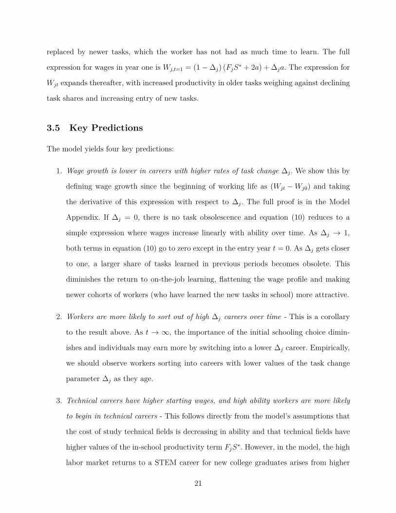
3.5 Key Predictions

The model yields four key predictions:

1. Wage growth is lower in careers with higher rates of task change ∆j. We show this by

defining wage growth since the beginning of working life as (Wjt −Wj0) and taking

the derivative of this expression with respect to ∆j. The full proof is in the Model

Appendix. If ∆j = 0, there is no task obsolescence and equation (10) reduces to a

simple expression where wages increase linearly with ability over time. As ∆j → 1,

both terms in equation (10) go to zero except in the entry year t = 0. As ∆j gets closer

to one, a larger share of tasks learned in previous periods becomes obsolete. This

diminishes the return to on-the-job learning, flattening the wage profile and making

newer cohorts of workers (who have learned the new tasks in school) more attractive.

2. Workers are more likely to sort out of high ∆j careers over time - This is a corollary

to the result above. As t → ∞, the importance of the initial schooling choice dimin-

ishes and individuals may earn more by switching into a lower ∆j career. Empirically,

we should observe workers sorting into careers with lower values of the task change

parameter ∆j as they age.

3. Technical careers have higher starting wages, and high ability workers are more likely

to begin in technical careers - This follows directly from the model’s assumptions that

the cost of study technical fields is decreasing in ability and that technical fields have

higher values of the in-school productivity term FjS∗. However, in the model, the high

labor market returns to a STEM career for new college graduates arises from higher

21

in-school learning as well as ability sorting. We test the relative importance of these

two explanations using data on ability on college major choice from the NLSY.

4. Higher ability workers are more likely to sort out of high ∆j careers over time - Many

other studies have found that STEM majors are positively selected on ability (e.g.

Altonji, Blom and Meghir 2012, Kinsler and Pavan 2015, Arcidiacono et al. 2016). A

less obvious prediction of the model is that high ability workers who start in STEM

careers are more likely to switch out of STEM careers over time. The Model Appendix

develops a simple three-period model that allows for endogenous schooling choices and

sorting across careers over time. We find that among workers who initially choose

STEM careers, those with the highest ability are more likely to sort out of STEM over

time. Intuitively, the return to ability is higher in careers where more of the gains from

on-the-job learning accumulate over time, and so higher-ability workers are more likely

to pay the short-run cost of switching out of STEM in order to recoup longer-run gains.

The Model Appendix proves this result and shows the intuition in Figure M.A1.

Section 4 presents empirical evidence that supports each of these predictions.

To develop some intuition for the model’s results, Figure 4 presents a simple simulation of

worker wage profiles, holding different elements of Wjt constant. Panel A shows the impacts

of field of study and career choice at different points in the life cycle. The solid blue line

represents a career with high initial productivity (FjS∗ = 6) and a relatively high rate of

task change (∆j = 0.2).25 With high starting wages and a high rate of task change, we can

think of the solid blue line as a STEM career.

The dashed red line shows the impact of reducing FjS∗ by half, holding ∆j constant.

This leads to a large initial difference in wages that narrows over time, with the two curves

intersecting as t → ∞. Intuitively, tasks learned in school gradually disappear from the

production function, leaving only the newer vintages and diminishing the impact of the25We fix a = 2 in all three scenarios.

22

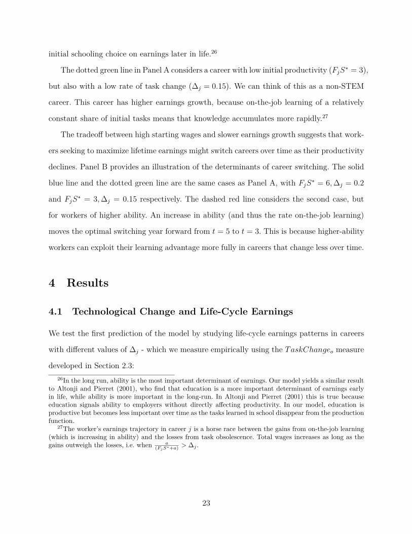
initial schooling choice on earnings later in life.26

The dotted green line in Panel A considers a career with low initial productivity (FjS∗ = 3),

but also with a low rate of task change (∆j = 0.15). We can think of this as a non-STEM

career. This career has higher earnings growth, because on-the-job learning of a relatively

constant share of initial tasks means that knowledge accumulates more rapidly.27

The tradeoff between high starting wages and slower earnings growth suggests that work-

ers seeking to maximize lifetime earnings might switch careers over time as their productivity

declines. Panel B provides an illustration of the determinants of career switching. The solid

blue line and the dotted green line are the same cases as Panel A, with FjS∗ = 6,∆j = 0.2

and FjS∗ = 3,∆j = 0.15 respectively. The dashed red line considers the second case, but

for workers of higher ability. An increase in ability (and thus the rate on-the-job learning)

moves the optimal switching year forward from t = 5 to t = 3. This is because higher-ability

workers can exploit their learning advantage more fully in careers that change less over time.

4 Results

4.1 Technological Change and Life-Cycle Earnings

We test the first prediction of the model by studying life-cycle earnings patterns in careers

with different values of ∆j - which we measure empirically using the TaskChangeo measure

developed in Section 2.3:26In the long run, ability is the most important determinant of earnings. Our model yields a similar result

to Altonji and Pierret (2001), who find that education is a more important determinant of earnings earlyin life, while ability is more important in the long-run. In Altonji and Pierret (2001) this is true becauseeducation signals ability to employers without directly affecting productivity. In our model, education isproductive but becomes less important over time as the tasks learned in school disappear from the productionfunction.

27The worker’s earnings trajectory in career j is a horse race between the gains from on-the-job learning(which is increasing in ability) and the losses from task obsolescence. Total wages increases as long as thegains outweigh the losses, i.e. when a

(FjS∗+a) > ∆j .

23

ln (earn)it = αit +A∑a

βaait +A∑a

γa (ait ∗ TaskChangeoit) + δXit + θt + ϵit (11)

This follows a similar format to equation (1) and Figure 1, except that instead of

using indicators for STEM major we directly interact the technological change measure

TaskChangeo with two-year age bins. The results are in Figure 5. We present separate

estimates of equation (11) for STEM and non-STEM occupations. As in Figure 1, the γ

coefficients can be interpreted as the relative earnings return to jobs with higher rates of

technological change, for each age group.

We find the same life-cycle patterns as in Figures 1, 2 and 3 - jobs with higher rates of

task change have flatter age-earnings profiles. The estimates imply that occupations with a

one standard deviation higher value of TaskChangeo (0.056) pay 15 percent higher wages

at ages 23-24 but only 4.5 percent higher wages at ages 39-40.

Importantly, this pattern holds equally for STEM and non-STEM occupations. While

the scale is different because STEM jobs have higher average values of TaskChangeo, the

pattern of declining returns over the first decade of working life is clear in both cases. Thus

the relationship between technological change and higher relative wages for recent college

graduates appears to be a general phenomenon that is not limited to STEM. Appendix

Figure A11 shows that these results are robust to controlling for industry fixed effects.

Appendix Figure A12 shows that we find a life-cycle pattern in wage returns when we

calculate TaskChangeo using only measures of software usage. Finally, Appendix Figure

A13 shows similar results when separating the sample by STEM/non-STEM majors rather

than STEM/non-STEM jobs.

Figure 6 tests the second prediction of the model by studying occupational sorting di-

rectly. We estimate:

TaskChangeoit = αit +

a=49,50∑a=23,24

βaait + δXit + θt + ϵit (12)

24

Equation (12) asks whether young people are relatively more likely to be employed in

occupations with high rates of technological change. One issue is that workers move up the

occupational ladder as they age, and higher-paying professional occupations also tend to have

higher values of TaskChangeo. To account for occupational upgrading, Figure 6 presents two

different estimates of equation (12). The first restricts the sample to professional occupations,

while the second restricts the sample to STEM majors.

The dashed line in Figure 6 shows that professional occupations with higher values of

TaskChangeo have younger workforces. The estimates imply that workers in jobs with a one

standard deviation higher value of TaskChangeo are about 1 percentage point more likely

to be ages 25-26 than ages 39-40. Since each two-year age group comprises about 7 percent

of our sample, a 1 percentage point difference is large relative to a baseline where all age

groups are evenly distributed across occupations.

The solid line in Figure 6 restricts the sample to STEM majors, regardless of occupation.

We find a very similar pattern. The difference between age 25-26 and age 39-40 implies that

STEM majors in jobs with a one standard deviation higher value of TaskChangeo are about

1.5 percentage points more likely to be ages 25-26 than ages 39-40. In results not reported,

we also find that this pattern holds for all workers (not just STEM majors) when we control

directly for the average wage of the occupation.

Overall, we find strong evidence of higher employment and relative wages for young work-

ers in jobs with higher rates of task change, confirming the first two predictions of the model.

Appendix Figure A14 shows that this pattern also holds when we measure TaskChangeo

using only software.

25

4.2 Accounting for Ability Differences by Major

We find that STEM majors are positively selected on ability, in both waves of the NLSY.28

This suggests that the high labor market return to a STEM degree might be confounded

by differences in academic ability across majors (e.g. Arcidiacono 2004, Kinsler and Pavan

2015). To account for ability differences, we estimate regressions of log wages on major choice,

using microdata from both waves of the NLSY:

ln (earn)it = αit + βASi + γPSi + δXit + ϵit (13)

The Xit vector includes controls for race, years of completed education, an indicator

variable for NLSY wave, and age and year fixed effects. The unit of observation in the

NLSY is a person-year, with standard errors clustered at the individual level. The sample is

restricted to ages 23-34 to ensure comparability across survey waves.

Column 1 of Table 3 presents results from the basic model in equation (13). Applied Sci-

ence majors earn about 18 percent more per year than non-STEM majors, while Pure Science

majors earn 10 percent less. Column 2 adds controls for cognitive skills (i.e. AFQT score),

social skills and “non-cognitive” skills.29 While each skill measure strongly and independently

predicts wages, adding them as controls does not meaningfully change the earnings premia

for both types of STEM majors. This suggests that higher wages in STEM careers cannot

be explained only by ability sorting.

Column 3 adds an indicator variable for employment in a STEM occupation. Earnings are

about 24 percent higher for STEM workers, regardless of major. Controlling for occupation

choice lowers the return to holding an Applied Science degree from 18 percent to 7 percent.

Column 4 adds industry fixed effects, which further shrinks the premium for Applied Science

majors to 3.4 percent.28Appendix Table A3 presents results that regress AFQT score on indicators for major type and major

interacted with NLSY wave. We find that STEM majors of both type score about 0.08 standard deviationshigher on the AFQT than non-STEM majors, but that this has not changed significantly across NLSY waves.

29We adopt the measures of social and “non-cognitive” skills from Deming (2017).

26

Column 5 adds interactions between STEM majors and STEM occupations. After con-

trolling for ability, Applied Science majors in non-STEM jobs earn only about 1.3 percent

more than non-STEM majors, and the difference is statistically insignificant. Non-STEM

majors in STEM jobs continue to earn a premium of about 12 percent (p<0.001), compared

to 19 percent for Applied Science majors in STEM jobs. The interaction term is statisti-

cally insignificant, suggesting that wages in STEM jobs are similar for workers with different

majors. Finally, Column 6 estimates the return to college major controlling for ability and

occupation-by-industry fixed effects, yielding coefficients on both STEM major types that

are statistically indistinguishable from zero.

In our model, high ability workers are more likely to major in STEM because they have

a lower cost of learning technical subjects. Yet higher earnings in STEM fields are driven

by the specific human capital accumulated in school, not by ability directly. The pattern of

results in Table 3 is consistent with our model, and inconsistent with a simpler story where

ability alone determines both major choice and earnings. Our results are also consistent with

Kinsler and Pavan (2015), who show that most of the return to a science major is driven by

the higher return to working in a closely-related job.

We also test whether the pattern of declining returns for STEM majors shown in Figures

1-3 holds when controlling for worker skills. The results are in Figure 7. Across both NLSY

waves, Applied Science majors earn about 21-24 percent more than non-STEM majors at

ages 23-26, compared to only about 5-12 percent at ages 31-34, a difference that is jointly

significant at the 5 percent level (p=0.041) despite the relatively small sample sizes in the

NLSY.

4.3 High ability workers sort out of STEM over time

The final prediction of the model is that high-ability workers will sort out of STEM careers

over time. The intuition is the returns to being a fast learner are greater in jobs with lower

rates of task change. Put another way, jobs with high rates of skill change erode the advantage

27

gained by learning more skills in each period on the job. Empirically, we should observe high

ability workers sorting into STEM careers initially, but sorting out of STEM careers later in

life. We test this by using the NLSY to estimate regressions of the form:

yit = αit + AGEit + βSTEMi + γAFQTi + θAGEi ∗ AFQTi + δXit + ϵit (14)

where AGEitis a linear age control for worker i in year t (scaled so that age 23=0, for

ease of interpretation), STEMi is an indicator for STEM major, and AGEi ∗AFQTi is the

interaction between age and cognitive ability. The Xit vector includes controls for race, years

of completed education, an indicator variable for NLSY wave, year fixed effects and cognitive,

social and non-cognitive skills. As with other results using the NLSY, the age range is 23-34,

observations are in person-years and we cluster standard errors at the individual level.

The results are in Table 4. The outcome in Columns 1 and 2 is an indicator for working

in a STEM occupation. Column 1 presents the baseline estimate of equation (14). We find

a positive and statistically significant coefficient on AFQTi but a negative and statistically

significant coefficient on the interaction term AGEi ∗ AFQTi. This confirms the prediction

that high-ability workers sort into STEM jobs initially but sort out over time. The results

imply that a worker with cognitive ability one standard deviation above average is 8.4 per-

centage points more likely to work in STEM at age 23, but only 3 percentage points more

likely to be working in an STEM job by age 34.

Column 2 studies sorting in more detail by adding AGEit ∗STEMi, AGEit ∗AFQTi and

AGEit ∗ STEMi ∗ AFQTi interactions to equation (14). This tests whether ability sorting

in and out of STEM occupations is different for STEM majors. We find that it is not -

the coefficient on the triple interaction AGEit ∗ STEMi ∗ AFQTi is almost exactly zero,

suggesting that the pattern of ability sorting holds regardless of major.

Columns 3 and 4 of Table 4 repeat the pattern above, except with log wages as the

outcome. Column 3 shows that there is a positive overall return to ability and that it is

increasing in age, consistent with the basic framework of the model. Column 4 adds the

28

interactions above. We find that the the coefficient on the key triple interaction term AGEit∗

STEMi ∗ AFQTi is large and negative, implying that the return to ability is much flatter

over time for STEM majors.

Summing the coefficients in Column 4 suggests that for a worker with cognitive ability one

standard deviation above average, STEM majors earn about 21 percent more than average at

age 23 and 40 percent more at age 35. In contrast, non-STEM majors of equal ability earn a

2 percent return at age 23 that grows rapidly to a 39 percent premium at age 35, completely

erasing the earnings advantage for STEM majors. Similar computations for AFQTi > 1

imply an earlier crossing point, an empirical result that is predicted by the stylized model

simulation in Figure 4B.

Thus the results in Table 4 confirm the fourth prediction of the model that high-ability

college graduates will choose STEM fields initially and exit for lower ∆j careers over time.

In results not reported, we show very similar results when we substitute STEM majors for

STEM occupations in Columns 3 and 4.30

5 Job Task Change in Earlier Periods

Our model predicts that increases in the rate of task change ∆j should flatten the age-

earnings profile of careers. The empirical application in Section 4 was a comparison of STEM

and non-STEM careers, but the prediction should also hold within careers over time. Specif-

ically, periods of relatively rapid technological change such as the computer/IT revolution

of the 1980s should correspond to an increase in the rate of task change and a rising relative

return for young workers in STEM careers.

The BG data only allow us to calculate detailed measure of job task changes for the 2007-

2017 period. We study the impact of technological change in earlier years using a database

of classified job ads assembled by Atalay et al. (2018). Atalay et al. (2018) assemble the30All the interactions have the same sign, although the implied convergence rates are much slower, perhaps

because of endogenous switching across STEM and non-STEM occupations based on expected returns.

29

full text of job advertisements in the New York Times, Wall Street Journal and Boston

Globe between 1940 and 2000, and they create measures of job task content and relate job

title to SOC codes using a text processing algorithm.31 Atalay et al. (2018) map words and

phrases to widely-used existing task content measures such as the Dictionary of Occupational

Titles (DOT) and the Occupational Information Network (O*NET), as well as the job task

classification schema used in past studies such as Autor et al. (2003), Spitz-Oener (2006),

Firpo et al. (2011) and Deming and Kahn (2018).

We estimate a version of TaskChangeo from equation (2) using the Atalay et al. (2018)

data and job task classifications.32 Since there is no natural mapping between our BG data

and the classified ads collected by Atalay et al (2018), we cannot create a directly comparable

measure. Our preferred approach is to use all of the task measures computed by Atalay et al.

(2018), although the results are not sensitive to other choices.33 We calculate TaskChangeo

for 5 year periods starting with 1973-1978 and ending with 1993-1998. Finally, to account

for fluctuations in the data we smooth each beginning and end point into a 3 year moving

average (e.g. 1998 is actually 1997-1999). 5 year bins starting with 1973-1978 and through

1993-1998.

We calculate TaskChangeo for each time period and occupation (6 digit SOC code) in

the Atalay et al. (2018) data, and then compute the vacancy-weighted average in each period

for STEM and non-STEM occupations. The results - in Panel A of Figure 7 - show three

main findings. First, the rate of task change for non-STEM occupations is relatively constant

at around 0.4 in each period.31Atalay et al. (2018)use a model called Continuous Bag of Words (CBOW), which finds synonyms for

words and phrases based how often they each appear next to similar words and phrases. The example given inAtalay et al. (2018) is as follows: “For example, to the extent that ’iv nurse,’ ’icu nurse,’ and ’rn coordinator’all tend to appear next to words like ’patient’,’care’, or ’blood’ one would conclude that ’rn’ and ’nurse’ havesimilar meanings to one another.” The exact CBOW model estimation details are in Appendix C.3 of Atalayet al. (2018).

32The data and programs can be found on the authors’ public data page -https://ssc.wisc.edu/~eatalay/occupation_data.html

33The BG data are much richer and more detailed than the classified ad data from Atalay et al. (2018).We use the largest number of skills to maximize comparability to later periods, while recognizing that onlycomparisons within datasets are trustworthy. Other approaches such as using only DOT and/or O*NET, oronly the skill measures that we can find in both data sources, yield broadly similar results.

30

Second, the rate of task change in STEM occupations fluctuates markedly, with peaks

that occur during the technological revolution of the 1980s. The TaskChangeo measure

more than doubles from 0.26 to 0.53 between the 1973-1978 and 1978-1983 periods, and

then increases again to 0.73 for 1983-1988 before falling again during the 1990s. Card and

DiNardo (2002) date the beginning of the “computer revolution” to the introduction of the

IBM-PC in 1981, and Autor et al. (1998) document a rapid increase in computer usage at

work starting in the 1980s.

Third, while 2007-2017 cannot be easily compared to earlier periods in levels due to

differences in the data, it is notable that the relatively higher value of TaskChangeo for

STEM occupations holds for the 2007-2017 period and the 1980s, but not the late 1970s

or 1990s. This suggests that new technologies may diffuse first through STEM occupations

before spreading gradually throughout the rest of the economy.

Our model predicts that periods with higher rates of task change will yield relatively

higher labor market returns for younger workers, especially in STEM occupations. We test

this by lining up the evidence in Panel A of Figure 7 with wage trends for young workers in

STEM jobs over the same period, using the CPS for years 1974-2016. We estimate population-

weighted regressions of the form:

ln (earn)it = αit+C∑c

γc (cit ∗ Yit)+C∑c

ζc (cit ∗ STit)+C∑c

ηc (cit ∗ Yit ∗ STit)+δXit+ϵit (15)

where cit is an indicator function I (year = c)it that is equal to one if respondent i is in

each of the five-year age bins starting with 1974-1978 and extending to 2009-2016 (with the

last period being slightly longer to maximize overlap with the BG data). Yit is an indicator

function that is equal to one if the respondent is “young”, defined as between the ages of

23 and 26 in the year of the survey, and STit is an indicator for whether the respondent is

working in a STEM occupation. The X vector includes controls for race and ethnicity, years

31

of completed education, and age and year fixed effects, as well as controls for the main effects

cit and STEMit. Thus the γ and ζ coefficients represent the wage premium for young workers

and older STEM workers relative to the base period of 1974-1978, while the η coefficients

represent the earnings premium for young STEM workers relative to older STEM workers

in each period.

The results are in Panel B of Figure 7. Each bar displays coefficients and 95% confidence

intervals for estimates of γ, ζ and η in equation (15). Comparing the timing to Panel A,

we see that the relative return to STEM for young workers is highest in periods with the

highest rate of task change. The premium for STEM workers age 23-26 relative to ages 27-50

is small and close to zero during the 1974-1978 period (when TaskChangeo in Panel A was

low), but jumps up to 18 percent and 24 percent in the 1979-1983 and 1983-1988 periods

respectively. It then falls to 16 percent for 1989-1993 and 8 percent for 1994-1998, exactly

when the rate of change falls again in Panel A.

Thus the results in Figure 7 confirm the predictions of the model that young STEM

workers earn relatively higher wages during periods of rapid task change, when their skills

are newer and relatively more valuable.34 In contrast, we do not find similar patterns of

fluctuating wage premia for older STEM workers (the second set of bars) or for young workers

in non-STEM occupations. The main effect of STEMit implies an overall wage premium of

around 24 percent for STEM occupations, but this changes very little over the 1974-2016

period.

Similarly, we find no consistent evidence that wages for young non-STEM workers move

in any systematic way with the rate of occupational task change. Finally, although we do

not have the data to calculate TaskChangeobetween 2000 and 2007, we find that a very

high return for young STEM workers during the 1999-2003 period, which coincides with the34One limitation of the CPS is that we do not know college major, and so it is possible that the patterns

we find are driven by selection of high-ability workers (including those who did not major in STEM) intoSTEM jobs. However, this would not by itself explain why selection would only occur among younger workers.Grogger and Eide (1995) show that about 25 percent of the rise in the college premium during the 1980scan be accounted for by an increase in the STEM skills acquired in college.

32

technology boom of the late 1990s (e.g. Beaudry et al. 2016).

6 Conclusion

This paper presents new evidence on the life-cycle returns to STEM education. We show that

the economic payoff to majoring in applied STEM fields such as engineering and computer

science is initially very high, but declines by more than 50 percent in the first decade after

college. STEM majors have flatter age-earnings profiles than college graduates who major in

other subjects, even after controlling for cognitive ability and other important determinants

of earnings.

We argue that the lower return to experience in STEM fields is due to the changing nature

of STEM jobs themselves. We calculate detailed measures of job task requirements using job

vacancy postings over the 2007-2017 period, and show that STEM jobs have relatively high

rates of job task change over the most recent decade. Both STEM and non-STEM occupations

that rank higher on our new measure of job task change employ younger workforces, and

have flatter age-earnings profiles.

We formalize the key mechanism of job task change with a simple model of education

and career choice. Intuitively, on-the-job learning is more difficult in careers where the job

functions themselves are constantly changing. Although STEM majors gain an initial earn-

ings advantage because they learn job-relevant skills in school, the advantage is eroded over

time by the introduction of new job tasks that make the old one obsolete. Our model predicts

that the highest-ability individuals will major in STEM and enter STEM careers initially,

but that they will be more likely to exit STEM over time. We find strong support for this

prediction using longitudinal data from the NLSY.

We use historical data on job vacancies assembled by Atalay et al. 2018 to test whether

the predictions of our framework hold during earlier periods, such as the computer and IT

revolution of the 1980s. We find large increases in the rate of task change for STEM jobs

33

during the 1980s, a period that coincides closely with important technological developments

such as the introduction of the personal computer. We also show that relative wages spiked

during this period for young STEM workers, a finding that is supported by the predictions

of the model.

This paper contributes to the ongoing policy debate over the “STEM shortage” by show-

ing that it is the new job-relevant skills that are scarce, not necessarily the STEM workers

themselves. In fact, faster technological progress contributes directly to the perception of

skill shortages by hastening skill obsolescence among older workers. Our approach of us-

ing vacancy data to measure job task change also makes a contribution to the study of

technological change, to the extent that progress manifests itself in the changing nature of

work.

Finally, our results inform policy tradeoffs between investment in specific and general edu-

cation. The high-skilled vocational preparation provided by STEM degrees paves a smoother

transition for college graduates entering the workforce. Yet at the same time, rapid techno-

logical change can lead to a short shelf life for technical skills. The rise of coding bootcamps,

stackable credentials and other attempts at “lifelong learning” can be seen as a market

response to anticipated skill obsolescence (Selingo 2018). This tradeoff between technology-

specific and general skills is an important consideration for policymakers and colleges seeking

to educate the workers of today, while also building the skills of the next generation.

References

Acemoglu, D. and Autor, D.: 2011, Skills, tasks and technologies: Implications for employ-

ment and earnings, Handbook of labor economics, Vol. 4, Elsevier, pp. 1043–1171. 3.1

Altonji, J. G., Arcidiacono, P. and Maurel, A.: 2016, The analysis of field choice in college and

graduate school: Determinants and wage effects, Handbook of the Economics of Education,

Vol. 5, Elsevier, pp. 305–396. 1

34

Altonji, J. G., Bharadwaj, P. and Lange, F.: 2012, Changes in the characteristics of american

youth: Implications for adult outcomes, Journal of Labor Economics 30(4), 783–828. 2.1,

8

Altonji, J. G., Blom, E. and Meghir, C.: 2012, Heterogeneity in human capital investments:

High school curriculum, college major, and careers, Annu. Rev. Econ. 4(1), 185–223. 1, 4

Altonji, J. G., Kahn, L. B. and Speer, J. D.: 2016, Cashier or consultant? entry labor market

conditions, field of study, and career success, Journal of Labor Economics 34(S1), S361–

S401. 2.1

Altonji, J. G. and Pierret, C. R.: 2001, Employer learning and statistical discrimination, The

Quarterly Journal of Economics 116(1), 313–350. 26

Arcidiacono, P.: 2004, Ability sorting and the returns to college major, Journal of Econo-

metrics 121(1-2), 343–375. 1, 4.2

Arcidiacono, P., Aucejo, E. M. and Hotz, V. J.: 2016, University differences in the gradu-

ation of minorities in stem fields: Evidence from california, American Economic Review

106(3), 525–62. 1, 4

Arora, A., Branstetter, L. G. and Drev, M.: 2013, Going soft: How the rise of software-based

innovation led to the decline of japan’s it industry and the resurgence of silicon valley,

Review of Economics and Statistics 95(3), 757–775. 2.3

Atalay, E., Phongthiengtham, P., Sotelo, S. and Tannenbaum, D.: 2018, The evolving us

occupational structure. 1, 5, 31, 33, 6

Aubert, P., Caroli, E. and Roger, M.: 2006, New technologies, organisation and age: firm-level

evidence, The Economic Journal 116(509). 1

Autor, D. and Dorn, D.: 2013, The growth of low-skill service jobs and the polarization of

the us labor market, American Economic Review 103(5), 1553–97. 2.1

35

Autor, D. H. and Handel, M. J.: 2013, Putting tasks to the test: Human capital, job tasks,

and wages, Journal of Labor Economics 31(S1), S59–S96. 2.3

Autor, D. H., Katz, L. F. and Krueger, A. B.: 1998, Computing inequality: have computers

changed the labor market?, The Quarterly Journal of Economics 113(4), 1169–1213. 5

Autor, D. H., Levy, F. and Murnane, R. J.: 2002, Upstairs, downstairs: Computers and skills

on two floors of a large bank, ILR Review 55(3), 432–447. 1

Autor, D. H., Levy, F. and Murnane, R. J.: 2003, The skill content of recent technological

change: An empirical exploration, The Quarterly journal of economics 118(4), 1279–1333.

1, 2.3, 5

Bartel, A., Ichniowski, C. and Shaw, K.: 2007, How does information technology affect pro-

ductivity? plant-level comparisons of product innovation, process improvement, and worker

skills, The quarterly journal of Economics 122(4), 1721–1758. 1

Beaudry, P., Green, D. A. and Sand, B. M.: 2016, The great reversal in the demand for skill

and cognitive tasks, Journal of Labor Economics 34(S1), S199–S247. 5

Black, S. E., Schanzenbach, D. W. and Breitwieser, A.: 2017, The recent decline in women’s

labor force participation, Driving Growth through Women’s Economic Participation p. 5.

2.1

Branstetter, L. G., Drev, M. and Kwon, N.: 2018, Get with the program: Software-driven

innovation in traditional manufacturing, Management Science . 2.3

Bresnahan, T. F., Brynjolfsson, E. and Hitt, L. M.: 2002, Information technology, workplace

organization, and the demand for skilled labor: Firm-level evidence, The Quarterly Journal

of Economics 117(1), 339–376. 1

Cappelli, P. H.: 2015, Skill gaps, skill shortages, and skill mismatches: Evidence and argu-

ments for the united states, ILR Review 68(2), 251–290. 1

36

Card, D. and DiNardo, J. E.: 2002, Skill-biased technological change and rising wage in-

equality: Some problems and puzzles, Journal of labor economics 20(4), 733–783. 1, 5

Carnevale, A. P., Cheah, B. and Strohl, J.: 2012, College Majors, Unemployment and Earn-

ings: Not all college degrees are created equal, Georgetown University Center on Educaiton

and the Workforce. 1

Carnevale, A. P., Smith, N. and Melton, M.: 2011, Stem: Science technology engineering

mathematics., Georgetown University Center on Education and the Workforce . 1, 2.1

Caselli, F.: 1999, Technological revolutions, American economic review 89(1), 78–102. 1, 3.3

Charette, R. N.: 2013, The stem crisis is a myth, IEEE Spectrum 50(9), 44–59. 1

Chari, V. V. and Hopenhayn, H.: 1991, Vintage human capital, growth, and the diffusion of

new technology, Journal of political Economy 99(6), 1142–1165. 1, 2, 3.3

Deming, D. J.: 2017, The growing importance of social skills in the labor market, The Quar-

terly Journal of Economics 132(4), 1593–1640. 1, 2.3, 2.3, 29

Deming, D. and Kahn, L. B.: 2018, Skill requirements across firms and labor markets: Evi-

dence from job postings for professionals, Journal of Labor Economics 36(S1), S337–S369.

15, 2.3, 5

Firpo, S., Fortin, N. and Lemieux, T.: 2011, Occupational tasks and changes in the wage

structure. 1, 5

Friedberg, L.: 2003, The impact of technological change on older workers: Evidence from

data on computer use, ILR Review 56(3), 511–529. 1

Galenson, D. W. and Weinberg, B. A.: 2000, Age and the quality of work: The case of modern

american painters, Journal of Political Economy 108(4), 761–777. 3

37

Galor, O. and Tsiddon, D.: 1997, Technological progress, mobility, and economic growth,

The American Economic Review pp. 363–382. 1, 3.3

Goldin, C., Katz, L. F. and Kuziemko, I.: 2006, The homecoming of american college women:

The reversal of the college gender gap, Journal of Economic perspectives 20(4), 133–156.

2.1

Gould, E. D., Moav, O. and Weinberg, B. A.: 2001, Precautionary demand for education,

inequality, and technological progress, Journal of Economic Growth 6(4), 285–315. 2

Griliches, Z.: 1957, Hybrid corn: An exploration in the economics of technological change,

Econometrica, Journal of the Econometric Society pp. 501–522. 1

Griliches, Z.: 1992, Introduction to” output measurement in the service sectors”, Output

measurement in the service sectors, University of Chicago Press, pp. 1–22. 1

Grogger, J. and Eide, E.: 1995, Changes in college skills and the rise in the college wage

premium, Journal of Human Resources pp. 280–310. 34

Hanson, G. H. and Slaughter, M. J.: 2016, High-skilled immigration and the rise of stem

occupations in us employment, Technical report, National Bureau of Economic Research.

12

Hanushek, E. A., Schwerdt, G., Woessmann, L. and Zhang, L.: 2017, General education,

vocational education, and labor-market outcomes over the lifecycle, Journal of Human

Resources 52(1), 48–87. 1

Hastings, J. S., Neilson, C. A. and Zimmerman, S. D.: 2013, Are some degrees worth more

than others? evidence from college admission cutoffs in chile, Technical report, National

Bureau of Economic Research. 1

Hershbein, B. and Kahn, L. B.: 2018, Do recessions accelerate routine-biased technological

change? evidence from vacancy postings, American Economic Review 108(7), 1737–72. 15

38

Jones, C. I.: 1995, R & d-based models of economic growth, Journal of political Economy

103(4), 759–784. 1

Jovanovic, B. and Nyarko, Y.: 1996, Learning by doing and the choice of technology, Econo-

metrica 64(6), 1299–1310. 1

Kinsler, J. and Pavan, R.: 2015, The specificity of general human capital: Evidence from

college major choice, Journal of Labor Economics 33(4), 933–972. 1, 2.2, 4, 4.2, 4.2

Kirkeboen, L. J., Leuven, E. and Mogstad, M.: 2016, Field of study, earnings, and self-

selection, The Quarterly Journal of Economics 131(3), 1057–1111. 1

Kredler, M.: 2014, Experience vs. obsolescence: A vintage-human-capital model, Journal of

Economic Theory 150, 709–739. 1, 2

Krueger, D. and Kumar, K. B.: 2004, Skill-specific rather than general education: A reason

for us–europe growth differences?, Journal of economic growth 9(2), 167–207. 1

Leighton, M. and Speer, J.: 2017, Labor market returns to college major specificity. 1

MacDonald, G. and Weisbach, M. S.: 2004, The economics of has-beens, Journal of Political

Economy 112(S1), S289–S310. 1, 3

McDowell, J. M.: 1982, Obsolescence of knowledge and career publication profiles: Some

evidence of differences among fields in costs of interrupted careers, The American Economic

Review 72(4), 752–768. 1

Neal, D.: 1999, The complexity of job mobility among young men, Journal of Labor Eco-

nomics 17(2), 237–261. 3.1

Neal, D. A. and Johnson, W. R.: 1996, The role of premarket factors in black-white wage

differences, Journal of political Economy 104(5), 869–895. 2.1

39

Nelson, R. R. and Phelps, E. S.: 1966, Investment in humans, technological diffusion, and

economic growth, The American economic review 56(1/2), 69–75. 3.3

Neuman, S. and Weiss, A.: 1995, On the effects of schooling vintage on experience-earnings

profiles: Theory and evidence, European economic review 39, 943–955. 1

Parente, S. L.: 1994, Technology adoption, learning-by-doing, and economic growth, Journal

of economic theory 63(2), 346–369. 1

Pavan, R.: 2011, Career choice and wage growth, Journal of Labor Economics 29(3), 549–587.

3.1

Peri, G., Shih, K. and Sparber, C.: 2015, Stem workers, h-1b visas, and productivity in us

cities, Journal of Labor Economics 33(S1), S225–S255. 1, 2.1, 4

Ransom, T.: 2016, Selective migration, occupational choice, and the wage returns to college

majors. 1

Rosen, S.: 1975, Measuring the obsolescence of knowledge, Education, income, and human

behavior, NBER, pp. 199–232. 1

Ruggles, S., Genadek, K., Goeken, R., Grover, J. and Sobek, M.: 2017, Integrated public use

microdata series: Version 6.0 [dataset]. minneapolis: University of minnesota, 2015. 2.1

Ryan, P.: 2001, The school-to-work transition: a cross-national perspective, Journal of eco-

nomic literature 39(1), 34–92. 1

Silos, P. and Smith, E.: 2015, Human capital portfolios, Review of Economic Dynamics

18(3), 635–652. 1

Spitz-Oener, A.: 2006, Technical change, job tasks, and rising educational demands: Looking

outside the wage structure, Journal of labor economics 24(2), 235–270. 5

40

Thompson, P.: 2003, Technological change and the age–earnings profile: Evidence from the

international merchant marine, 1861–1912, Review of Economic Dynamics 6(3), 578–601.

1

Violante, G. L.: 2002, Technological acceleration, skill transferability, and the rise in residual

inequality, The Quarterly Journal of Economics 117(1), 297–338. 1

Webber, D. A.: 2014, The lifetime earnings premia of different majors: Correcting for selection

based on cognitive, noncognitive, and unobserved factors, Labour economics 28, 14–23. 1

Weinberg, B. A.: 2004, Experience and technology adoption. 1

41

Age WagesShare in

STEM JobWages

Share in

STEM JobWages

Share in

STEM JobWages

Share in

STEM Job

(1) (2) (3) (4) (5) (6) (7) (8)

23 32,236 0.122 42,277 0.699 32,840 0.337 47,007 0.880

24 36,632 0.123 47,608 0.727 35,909 0.353 52,727 0.891

25 43,354 0.125 54,149 0.715 44,849 0.334 58,188 0.881

26 46,918 0.123 57,971 0.725 49,472 0.360 61,558 0.880

27 51,722 0.125 62,324 0.716 53,181 0.309 66,286 0.893

28 54,856 0.124 65,621 0.676 57,243 0.297 69,590 0.856

29 58,389 0.120 69,961 0.658 62,651 0.304 73,765 0.843

30 62,787 0.124 73,772 0.651 69,109 0.293 76,309 0.845

31 67,567 0.122 80,097 0.613 79,274 0.275 80,546 0.798

32 71,933 0.123 82,266 0.617 79,894 0.271 83,536 0.802

33 74,608 0.121 89,800 0.598 91,085 0.268 89,109 0.776

34 79,971 0.117 94,009 0.578 98,442 0.265 91,542 0.753

35 85,897 0.116 101,143 0.546 105,914 0.267 98,291 0.712

36 89,875 0.119 103,950 0.546 111,807 0.261 99,114 0.722

37 93,259 0.125 108,221 0.531 114,927 0.286 103,804 0.693

38 94,453 0.123 112,042 0.510 117,943 0.260 108,081 0.678

39 99,481 0.111 114,797 0.508 121,372 0.253 110,477 0.675

40 99,952 0.116 116,127 0.485 123,224 0.256 111,678 0.629

41 103,447 0.112 117,203 0.474 123,281 0.253 113,388 0.613

42 104,068 0.116 116,886 0.500 122,578 0.270 113,511 0.637

43 106,122 0.116 124,672 0.478 132,626 0.267 120,005 0.603

44 108,777 0.108 124,720 0.487 129,115 0.267 122,278 0.609

45 111,802 0.104 126,337 0.502 136,001 0.273 121,420 0.619

46 111,235 0.103 128,250 0.458 141,341 0.232 121,746 0.571

47 112,430 0.100 129,106 0.485 136,539 0.274 125,350 0.591

48 112,002 0.096 129,968 0.481 136,772 0.283 126,601 0.579

49 112,347 0.096 130,408 0.469 139,118 0.278 126,111 0.564

50 111,754 0.098 130,289 0.461 137,439 0.273 126,606 0.557

Table 1: Life-Cycle Earnings and Employment for STEM Majors

Notes: This table presents population-weighted average annual wage and salary income and employment shares in Science,

Technology, Engineering and Mathematics (STEM) occupations by age, using the 2009-2016 American Community Survey

Integrated Public Use Microdata Series (IPUMS, Ruggles et al 2017). The sample is restricted to men with at least a college

degree who were employed at the time of the survey and worked at least 40 weeks during the year. Earnings are in constant

2016 dollars. STEM majors are defined following Peri, Shih and Sparber (2015), and STEM jobs are defined using the 2010

Census Bureau classification. "Pure" Science includes biology, chemistry, physics, mathematics and statistics, while

"Applied" Science includes engineering and computer science.

Non-STEM Major STEM Major "Pure" Science "Applied" Science

SOC code Occupation TitleRate of Task

ChangeSOC code Occupation Title

Rate of Task

Change

231 Lawyers, Judges and Related Workers 0.239 173013 Mechanical Drafters 0.404

171 Architects and Surveyors 0.217 151131 Computer Programmers 0.355

192 Physical Scientists 0.207 173011 Architectural and Civil Drafters 0.344

191 Life Scientists 0.203 151133 Software Developers, Systems Software 0.301

172 Engineers 0.197 112011 Advertising and Promotions Managers 0.282

173 Drafters and Engineering Technicians 0.197 172081 Environmental Engineers 0.281

152 Mathematical Scientists 0.184 132053 Insurance Underwriters 0.281

113 Operations Specialties Managers 0.173 291051 Pharmacists 0.281

254 Librarians, Curators and Archivists 0.172 173012 Electrical and Electronics Drafters 0.274

232 Legal Support Workers 0.165 152011 Actuaries 0.244

SOC code Occupation TitleRate of Task

ChangeSOC code Occupation Title

Rate of Task

Change

193 Social Scientists and Related Workers 0.099 291065 Pediatricians 0.030

291 Health Diagnosing and Treating Practitioners 0.101 291171 Nurse Practitioners 0.050

252 Pre-K, Primary and Secondary School Teachers 0.104 291021 Dentists 0.052

259 Other Education, Training and Library Occupations 0.105 193031 Clinical Psychologists 0.054

253 Other Teachers and Instructors 0.109 291131 Veterinarians 0.054

292 Health Technologists and Technicians 0.117 292052 Pharmacy Technicians 0.056

111 Managers and Executives 0.122 252059 Special Education Teachers, All Other 0.056

194 Life, Physical and Social Science Technicians 0.126 291066 Psychiatrists 0.057

299 Other Healthcare Practitioners 0.128 291069 Physicians and Surgeons, All Other 0.063

211 Counselors and Social Workers 0.131 291151 Nurse Anesthetists 0.067

Notes: This table uses online job vacancy data from Burning Glass Technologies (BG) to calculate the rate of task change between 2007 and 2017 for each 3- and 6-digit

Standard Occupational Classification (SOC) code. The task change measure ranges between 0 and 1, with zero indicating that the tasks demanded by employers in the

occupation in 2007 were exactly the same as in 2017, and 1 indicating that the job has a completely different set of task demands. The average value of the task change

measure is 0.13 - see the text for details. Professional Occupations are SOC codes where the first digit begins with a 1 or a 2.

Table 2: Occupations with the Highest and Lowest Rates of Task Change

Panel B: Fastest-Changing Professional Occupations (6-digit)

Panel D: Slowest-Changing Professional Occupations (6-digit)Panel C: Slowest-Changing Professional Occupations (3-digit)

Panel A: Fastest-Changing Professional Occupations (3-digit)

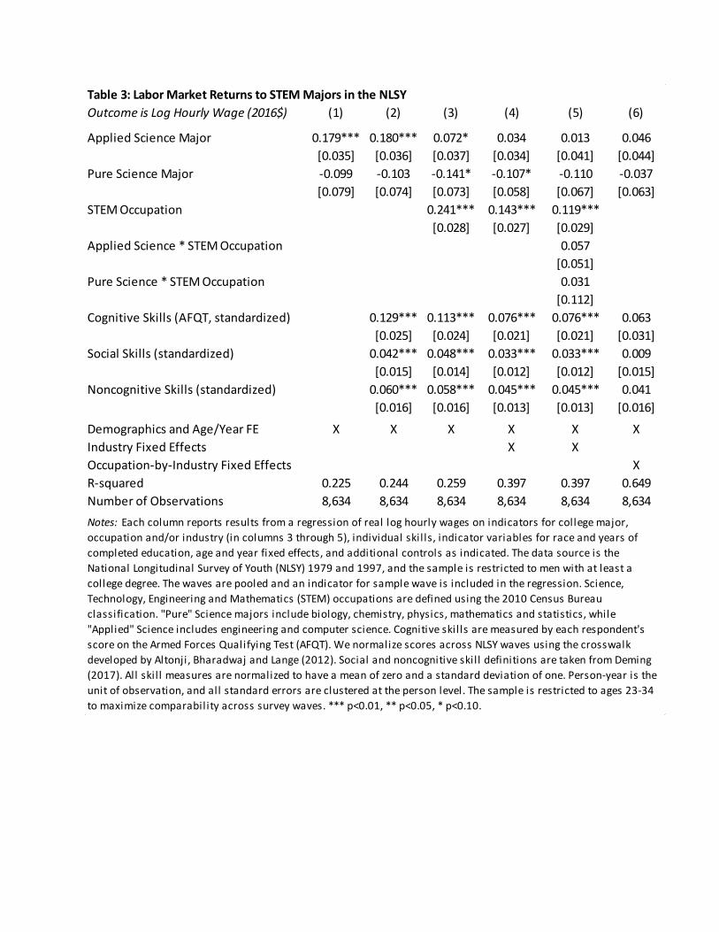
Table 3: Labor Market Returns to STEM Majors in the NLSY

Outcome is Log Hourly Wage (2016$) (1) (2) (3) (4) (5) (6)

Applied Science Major 0.179*** 0.180*** 0.072* 0.034 0.013 0.046

[0.035] [0.036] [0.037] [0.034] [0.041] [0.044]

Pure Science Major -0.099 -0.103 -0.141* -0.107* -0.110 -0.037

[0.079] [0.074] [0.073] [0.058] [0.067] [0.063]

STEM Occupation 0.241*** 0.143*** 0.119***

[0.028] [0.027] [0.029]

Applied Science * STEM Occupation 0.057

[0.051]

Pure Science * STEM Occupation 0.031

[0.112]

Cognitive Skills (AFQT, standardized) 0.129*** 0.113*** 0.076*** 0.076*** 0.063

[0.025] [0.024] [0.021] [0.021] [0.031]

Social Skills (standardized) 0.042*** 0.048*** 0.033*** 0.033*** 0.009

[0.015] [0.014] [0.012] [0.012] [0.015]

Noncognitive Skills (standardized) 0.060*** 0.058*** 0.045*** 0.045*** 0.041

[0.016] [0.016] [0.013] [0.013] [0.016]

Demographics and Age/Year FE X X X X X X

Industry Fixed Effects X X

Occupation-by-Industry Fixed Effects X

R-squared 0.225 0.244 0.259 0.397 0.397 0.649

Number of Observations 8,634 8,634 8,634 8,634 8,634 8,634

Notes: Each column reports results from a regression of real log hourly wages on indicators for college major,

occupation and/or industry (in columns 3 through 5), individual skil ls, indicator variables for race and years of

completed education, age and year fixed effects, and additional controls as indicated. The data source is the

National Longitudinal Survey of Youth (NLSY) 1979 and 1997, and the sample is restricted to men with at least a

college degree. The waves are pooled and an indicator for sample wave is included in the regression. Science,

Technology, Engineering and Mathematics (STEM) occupations are defined using the 2010 Census Bureau

classification. "Pure" Science majors include biology, chemistry, physics, mathematics and statistics, while

"Applied" Science includes engineering and computer science. Cognitive skil ls are measured by each respondent's

score on the Armed Forces Qualifying Test (AFQT). We normalize scores across NLSY waves using the crosswalk

developed by Altonji, Bharadwaj and Lange (2012). Social and noncognitive skil l definitions are taken from Deming

(2017). All skil l measures are normalized to have a mean of zero and a standard deviation of one. Person-year is the

unit of observation, and all standard errors are clustered at the person level. The sample is restricted to ages 23-34

to maximize comparability across survey waves. *** p<0.01, ** p<0.05, * p<0.10.

Table 4: STEM Majors, Relative Wages and Ability Sorting in the NLSY

(1) (2) (3) (4)

STEM Major 0.352*** 0.170*** 0.116*** 0.005

[0.035] [0.055] [0.034] [0.120]

AFQT (Standardized) 0.084*** 0.066*** 0.063* 0.017

[0.016] [0.014] [0.033] [0.032]

Age (Linear) 0.002 -0.001 0.013 0.007

[0.005] [0.004] [0.008] [0.009]

Age * AFQT -0.005** -0.006*** 0.013*** 0.024***

[0.002] [0.002] [0.005] [0.005]

Age * STEM Major 0.015* 0.027*

[0.008] [0.014]

STEM Major * AFQT 0.095** 0.187*

[0.048] [0.097]

STEM Major * AFQT * Age 0.000 -0.041***

[0.007] [0.013]

R-squared 0.183 0.190 0.237 0.242

Number of Observations 11,214 11,214 8,685 8,685

Notes: Each column reports results from a regression of indicators for working in a

STEM occupation (Columns 1 and 2) or real log hourly wages (Columns 3 and 4) on

indicators for majoring in a Science, Technology, Engineering and Mathematics (STEM)

field, cognitive, social and noncognitive skil ls, indicator variables for race and years of

completed education, year fixed effects, and additional controls as indicated. The data

source is the National Longitudinal Survey of Youth (NLSY) 1979 and 1997, and the

sample is restricted to men with at least a college degree. The waves are pooled and an

indicator for sample wave is included in the regression. STEM majors are defined

following Peri, Shih and Sparber (2015), and STEM occupations are defined using the

2010 Census Bureau classification. Cognitive skil ls are measured by each respondent's

score on the Armed Forces Qualifying Test (AFQT). We normalize scores across NLSY

waves using the crosswalk developed by Altonji, Bharadwaj and Lange (2012). Social

and noncognitive skil l definitions are taken from Deming (2017). All skil l measures are

normalized to have a mean of zero and a standard deviation of one. Person-year is the

unit of observation, and all standard errors are clustered at the person level. The

sample is restricted to ages 23-34 to maximize comparability across survey waves. ***

p<0.01, ** p<0.05, * p<0.10.

Ln (Wages)In a STEM Job

Figure 1

Notes: The figure plots coefficients and 95 percent confidence intervals from an estimate of the returns to majors

over time, following equation (1) in the paper. "Pure" Science includes biology, chemistry, physics, mathematics

and statistics, while "Applied" Science includes engineering and computer science.

-.1

0.1

.2.3

.4

25 30 35 40 45 50Age (2 -year bins)

2009-2016 American Community Survey

.5.3

.1-.

1

25 30 35 40 45 50Age (2 -year bins)

Applied Science Majors Pure Science Majors

Samples are full-time working men with a college degree; outcome is log wages

Left-out category is all other majors; includes demographic controls and age and year fixed effects

1993-2013 National Survey of College Graduates

Life-Cycle Returns to STEM Majors

Figure 2

Notes: The figure plots coefficients and 95 percent confidence intervals from three separate estimates of equation (1) in the paper, except we interact

age bins with indicators for working in a STEM occupation rather than earning a STEM degree. STEM occupations are defined using the 2010 Census

Bureau classification. The three data sources are the 2009-2016 American Community Survey, the 1993-2013 National Survey of College Graduates,

and the 1973-2016 Current Population Survey.

.1.2

.3.4

.5

25 30 35 40 45 50Age (2 -year bins)

ACS NSCG CPS

Sample is full-time working men with at least a college degree

Left-out category is all other majors; includes demographic controls and age and year fixed effects

Outcome is Log Wages

Life-Cycle Returns to Working in a STEM Occupation Across 3 Data Sources

Figure 3

Notes: The figure plots coefficients and 95 percent confidence intervals from an estimate of the returns to majors over time, following equation (1) in

the paper, but adding occupation and major interactions. "Applied" Science majors include engineering and computer science.

0.2

.4.6

25 30 35 40 45 50Age (2 -year bins)

Appl Sci, non-STEM job Other Major, STEM Job Appl Sci, STEM Job

Left-out category is other major, non-STEM job; includes demographic controls and age and year fixed effects

Sample is full-time working men with at least a college degree; 2009-2016 ACS

Outcome is Log Wages

Declining Returns for STEM Jobs, not STEM Majors

Figure 4A

Notes: This Figure simulates earnings growth from the model in Section 3 of the paper when 𝐹𝑗𝑆∗ = 6 (high in-school productivity) or 𝐹𝑗𝑆

∗ = 3 (low

in-school productivity) and the rate of task change ∆𝑗 is equal to 0.20 or 0.15. See the text for details.

Impact of schooling diminishes over time

High delta = lower earnings growth

FjS*+a

(1/2)FjS* + a

Wag

es (

Wjt)

0 5 10 15Years since graduation

High in-school productivity; delta=0.2

Low in-school productivity; delta=0.2

Low in-school productivity; delta=0.15

Figure 4B

Notes: This Figure simulates earnings growth from the model in Section 3 of the paper when 𝐹𝑗𝑆∗ = 6 (high in-school productivity) or 𝐹𝑗𝑆

∗ = 3 (low

in-school productivity), the rate of task change ∆𝑗 is equal to 0.20 or 0.15, and for a high vs. low ability worker. See the text for details.

High ability workers learn more on the job, switch earlier into low delta fields

FjS*+a

(1/2)FjS*+a

Wag

es (

Wjt)

0 5 10 15Years since graduation

High in-school productivity; delta=0.2

Low in-school productivity, delta=0.15

Low in-school productivity, higher ability, delta=0.15

Figure 5

Notes: The figure plots coefficients and 95 percent confidence intervals from equation (10) in the paper, a regression of log wages on interactions

between age and the task change measure ∆𝑗 that is estimated using 2007-2017 online job vacancy data from Burning Glass Technologies. STEM

occupations are defined using the 2010 Census Bureau classification. See the text for details.

2.5

1.5

.50

-.5

12

25 30 35 40 45 50Age (2-year bins)

STEM Occupations Non-STEM Occupations

Sample: Full-time working men with at least a college degree; 2009-2016 ACS

Iincludes demographic controls and age and year fixed effects; SD(task change) = 0.056

Wage Returns to Changing Task Demands in an Occupation

Jobs with Higher Rates of Task Change Pay More to Younger Workers

Figure 6

Notes: The figure plots coefficients and 95 percent confidence intervals from equation (11) in the paper, a regression of the task change measure ∆𝑗

(which is estimated using 2007-2017 online job vacancy data from Burning Glass Technologies) on occupation by age group interactions. STEM

occupations are defined using the 2010 Census Bureau classification. See the text for details.

-.0

02

5

0

.002

5.0

05

.007

5

.01

25 30 35 40 45 50Age (2-year bins)

All Majors; Professional Occupations STEM Majors

Sample: Full-time working men with at least a college degree; 2009-2016 ACS

Left-out category is age 49-50; includes demographic controls and age and year fixed effects

Outcome is the Task Change Measure

Jobs with Changing Task Demands Employ Younger Workers

Figure 7

Notes: The figure plots coefficients and 95 percent confidence intervals from an estimate of the returns to Applied Science majors over time, following

equation (1) in the paper. "Applied" Science includes engineering and computer science majors. The regression is estimated at the person-year level

and standard errors are clustered at the individual level. The sample is restricted to ages 23-34 to ensure comparability across NLSY waves.

-.1

0.1

.2.3

24 26 28 30 32 34Age (2 -year bins)

Sample is full-time working men with at least a college degree; NLSY79 and NLSY97 (Pooled)

Includes demographic controls, age and year fixed effects, AFQT and noncognitive skills

Outcome is Log Wages

Declining Life-Cycle Returns to Applied Science Majors

Figure 8

Notes: Panel A presents estimates of the task change measure ∆𝑗 calculated using data from Atalay et al (2018) on the text of classified job ads

between the years of 1977 and 1999. Panel B presents coefficients and 95 percent confidence intervals from a regression of log wages on age (23-26 vs. 27-50) by STEM occupation interactions for successive five year periods that match the job ad data, using the CPS. STEM occupations are defined using the 2010 Census Bureau classification. See the text for details.

Task data from text of classified ads, as in Atalay et al (2018)

Task data from online job vacancies, 2007-2017

0.2

.4.6

.8

1978 1983 1988 1993 1998 2017

Non-STEM Occupations STEM Occupations

Calculated over five year periods beginning with 1973-1978; see text for details

1973-1998 data taken from Atalay et al (2018); 2007-2017 data from Burning Glass

Rate of Within-Occupation Task Change, by Period

-.1

0.1

.2.3

1978 1983 1988 1993 1998 2003 2008 2016

Young STEM workers Older STEM workers Young non-STEM workers

Sample is full-time men with at least a college degree; 1973-2016 CPS

Outcome is log wages; includes controls for demographics and age and year fixed effects; "young" is age 23-26

Young STEM Workers Earn More During Periods of Rapid Task Change

Appendix Results

NOT FOR PUBLICATION

Table A1: Selection into Graduate School in the NLSY

Outcome is an indicator for graduate education (1) (2) (3)

Cognitive Skill (AFQT, standardized) 0.099*** 0.099*** 0.131***

[0.022] [0.022] [0.032]

STEM Major -0.034 -0.110*** -0.013

[0.032] [0.041] [0.073]

NLSY Wave 0.103*** 0.063** 0.089*

[0.027] [0.031] [0.051]

STEM Major * NLSY Wave 0.181*** 0.162

[0.064] [0.121]

AFQT * NLSY Wave -0.028

[0.044]

STEM Major * AFQT -0.100*

[0.062]

STEM Major * AFQT * NLSY Wave 0.027

[0.100]

R-squared 0.030 0.035 0.038

Number of Observations 1,360 1,360 1,360

Notes: Each column reports results from a regression of an indicator for graduate

school attendance on the Armed Forces Qualifying Test (AFQT) score, indicators for

college major, an indicator for whether the respondent is in the National Longitudinal

Survey of Youth (NLSY) 1997 survey wave, and other variables as shown. The regression

also includes controls for race. The sample pools the 1979 and 1997 NLSY waves

together and is restricted to men with at least a college degree. STEM majors are defined

following Peri, Shih and Sparber (2015). "Pure" Science majors include biology,

chemistry, physics, mathematics and statistics, while "Applied" Science includes

engineering and computer science. We normalize scores across NLSY waves using the

crosswalk developed by Altonji, Bharadwaj and Lange (2012). The sample is restricted to

ages 23-34 to maximize comparability across survey waves. *** p<0.01, ** p<0.05, *

p<0.10.

SOC code Occupation TitleSoftware

Task ChangeSOC code Occupation Title

Software Task

Change

171 Architects and Surveyors 0.062 151131 Computer Programmers 0.140

151 Computer Occupations 0.058 151133 Software Developers, Systems Software 0.133

173 Drafters and Engineering Technicians 0.030 151134 Web Developers 0.098

172 Engineers 0.030 173011 Architectural and Civil Drafters 0.094

152 Mathematical Scientists 0.029 173013 Mechanical Drafters 0.094

271 Art and Design Workers 0.028 271014 Multimedia Artists and Animators 0.076

273 Media and Communications Workers 0.025 151142 Network and Computer Systems Administrators 0.069

274 Media and Communications Equipment Workers 0.024 271024 Graphic Designers 0.067

131 Business Operations Specialists 0.022 151141 Database Administrators 0.065

132 Financial Specialists 0.019 151141 Software Developers, Applications 0.065

SOC code Occupation TitleSoftware

Task ChangeSOC code Occupation Title

Software Task

Change

291 Health Diagnosing and Treating Practitioners 0.002 291065 Pediatricians 0.000

252 Pre-K, Primary and Secondary School Teachers 0.004 291151 Nurse Anesthetists 0.000

253 Other Teachers and Instructors 0.004 292021 Dental Hygienists 0.001

292 Health Technologists and Technicians 0.004 291131 Veterinarians 0.001

211 Counselors and Social Workers 0.008 291171 Nurse Practitioners 0.001

251 Postsecondary Teachers 0.009 291066 Psychiatrists 0.001

259 Other Education, Training and Library Occupations 0.010 252011 Preschool Teachers 0.001

299 Other Healthcare Practitioners 0.010 291021 Dentists 0.001

191 Life Scientists 0.010 292055 Surgical Technologists 0.001

193 Social Scientists 0.010 291062 Family and General Practitioners 0.001

Notes: This table uses online job vacancy data from Burning Glass Technologies (BG) to calculate the rate of change for software-related tasks between 2007 and 2017 for

each 3- and 6-digit Standard Occupational Classification (SOC) code. The task change measure ranges between 0 and 1, with zero indicating that the tasks demanded by

employers in the occupation in 2007 were exactly the same as in 2017, and 1 indicating that the job has a completely different set of task demands. We restrict the set of

occupations in the table to those with at least 10,000 total vacancies posted in both 2007 and 2017. The average value of the software task change measure is 0.016 - see

the text for details. Professional Occupations are SOC codes where the first digit begins with a 1 or a 2.

Table A2: Occupations with the Highest and Lowest Rates of Software-Related Task Change

Panel A: Fastest-Changing Professional Occupations (3-digit) Panel B: Fastest-Changing Professional Occupations (6-digit)

Panel C: Slowest-Changing Professional Occupations (3-digit) Panel D: Slowest-Changing Professional Occupations (6-digit)

Table A3: Ability Sorting into STEM Majors in the NLSY

Outcome is AFQT Score (standardized) (1) (2) (3)

STEM Major 0.083** 0.076

[0.039] [0.051]

NLSY 97 Wave 0.048 0.044 0.051

[0.053] [0.056] [0.055]

STEM Major * NLSY Wave 0.019

[0.079]

Applied Science Major 0.083

[0.056]

Applied Science Major * NLSY Wave -0.021

[0.089]

R-squared 0.217 0.217 0.217

Number of Observations 1,360 1,360 1,360

Notes: Each column reports results from a regression of the Armed Forces Qualifying

Test (AFQT) score on indicators for college major and an indicator for whether the

respondent is in the National Longitudinal Survey of Youth (NLSY) 1997 survey wave.

The regression also includes controls for race and the age at which the test was taken.

The sample pools the 1979 and 1997 NLSY waves together and is restricted to men

with at least a college degree. STEM majors are defined following Peri, Shih and

Sparber (2015). "Pure" Science majors include biology, chemistry, physics,

mathematics and statistics, while "Applied" Science includes engineering and

computer science. We normalize scores across NLSY waves using the crosswalk

developed by Altonji, Bharadwaj and Lange (2012). The sample is restricted to ages 23-

34 to maximize comparability across survey waves. *** p<0.01, ** p<0.05, * p<0.10.

Figure A1

Notes: The figure plots coefficients and 95 percent confidence intervals from an estimate of the returns to majors over time for women, following

equation (1) in the paper. "Pure" Science includes biology, chemistry, physics, mathematics and statistics, while "Applied" Science includes

engineering and computer science.

-.1

0.1

.2.3

.4

25 30 35 40 45 50Age (2 -year bins)

Applied Science Majors Pure Science Majors

Sample is full-time working women with at least a college degree; 2009-2016 ACS

Left-out category is all other majors; includes demographic controls and age and year fixed effects

Outcome is Log Wages

Declining Life-Cycle Returns to Majoring in STEM

Figure A2

Notes: The figure plots coefficients and 95 percent confidence intervals from an estimate of equation (1) in the paper, except with an indicator for

working in a STEM occupation as the outcome. "Pure" Science includes biology, chemistry, physics, mathematics and statistics, while "Applied"

Science includes engineering and computer science. STEM occupations are defined using the 2010 Census Bureau classification.

0.2

.4.6

.8

25 30 35 40 45 50Age (2 -year bins)

Applied Science Majors Pure Science Majors

Sample is full-time working women with at least a college degree; 2009-2016 ACS

Left-out category is all other majors; includes demographic controls and age and year fixed effects

Outcome is an indicator for being employed in a STEM job

STEM Majors Less Likely to Work in STEM Jobs Over Time

Figure A3

Notes: The figure plots coefficients and 95 percent confidence intervals from an estimate of equation (1) in the paper, except with an indicator for

working in a STEM occupation as the outcome. "Pure" Science includes biology, chemistry, physics, mathematics and statistics, while "Applied"

Science includes engineering and computer science. STEM occupations are defined using the 2010 Census Bureau classification.

0.2

.4.6

.8

25 30 35 40 45 50Age (2 -year bins)

Applied Science Majors Pure Science Majors

Sample is full-time working men with at least a college degree; 2009-2016 ACS

Left-out category is all other majors; includes demographic controls and age and year fixed effects

Outcome is an indicator for being employed in a STEM job

STEM Majors Less Likely to Work in STEM Jobs Over Time

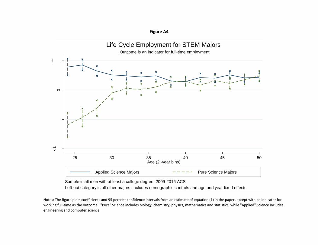
Figure A4

Notes: The figure plots coefficients and 95 percent confidence intervals from an estimate of equation (1) in the paper, except with an indicator for

working full-time as the outcome. "Pure" Science includes biology, chemistry, physics, mathematics and statistics, while "Applied" Science includes

engineering and computer science.

-.1

-.0

5

0

.05

25 30 35 40 45 50Age (2 -year bins)

Applied Science Majors Pure Science Majors

Sample is all men with at least a college degree; 2009-2016 ACS

Left-out category is all other majors; includes demographic controls and age and year fixed effects

Outcome is an indicator for full-time employment

Life Cycle Employment for STEM Majors

Figure A5

Notes: The figure plots coefficients and 95 percent confidence intervals from an estimate of equation (1) in the paper, except the sample includes all

working men (not just full-time). "Pure" Science includes biology, chemistry, physics, mathematics and statistics, while "Applied" Science includes

engineering and computer science.

-.2

0.2

.4.6

25 30 35 40 45 50Age (2 -year bins)

Applied Science Majors Pure Science Majors

Sample is all working men with at least a college degree; 2009-2016 ACS

Left-out category is all other majors; includes demographic controls and age and year fixed effects

Outcome is Log Wages

Life-Cycle Returns to STEM Majors

Figure A6

Notes: The figure plots coefficients and 95 percent confidence intervals from an estimate of equation (1) in the paper, except the sample is restricted

to full-time working men with exactly a bachelor’s degree. "Pure" Science includes biology, chemistry, physics, mathematics and statistics, while

"Applied" Science includes engineering and computer science.

-.1

0.1

.2.3

.4

25 30 35 40 45 50Age (2 -year bins)

Applied Science Majors Pure Science Majors

Sample is full-time working men with exactly a college degree; 2009-2016 ACS

Left-out category is all other majors; includes demographic controls and age and year fixed effects

Outcome is log wages

Life-Cycle Returns to STEM Majors

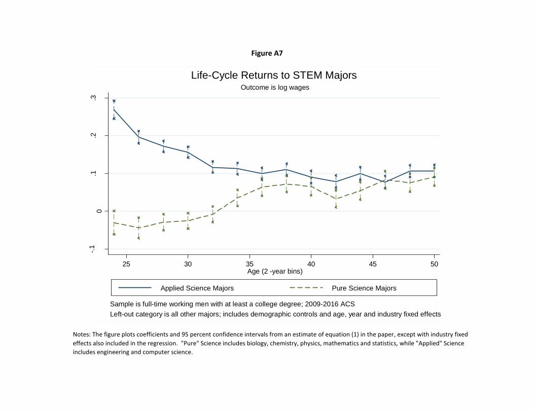
Figure A7

Notes: The figure plots coefficients and 95 percent confidence intervals from an estimate of equation (1) in the paper, except with industry fixed

effects also included in the regression. "Pure" Science includes biology, chemistry, physics, mathematics and statistics, while "Applied" Science

includes engineering and computer science.

-.1

0.1

.2.3

25 30 35 40 45 50Age (2 -year bins)

Applied Science Majors Pure Science Majors

Sample is full-time working men with at least a college degree; 2009-2016 ACS

Left-out category is all other majors; includes demographic controls and age, year and industry fixed effects

Outcome is log wages

Life-Cycle Returns to STEM Majors

Figure A8

Notes: The figure plots coefficients and 95 percent confidence intervals from an estimate of equation (1) in the paper. The definition of STEM majors

is taken from Peri, Shih and Sparber (2015).

.1.1

5.2

.25

.3

25 30 35 40 45 50Age (2 -year bins)

STEM Majors

Sample is full-time working men with at least a college degree; 2009-2016 ACS

Left-out category is all other majors; includes demographic controls and age and year fixed effects

Outcome is log wages

Life-Cycle Returns to STEM Majors

Figure A9

Notes: The figure plots coefficients and 95 percent confidence intervals from an estimate of equation (1) in the paper, except with Engineering and

Computer Science majors estimated separately.

.1.2

.3.4

.5

25 30 35 40 45 50Age (2 -year bins)

Engineering Majors Computer Science Majors

Sample is full-time working men with at least a college degree; 2009-2016 ACS

Left-out category is all other majors; includes demographic controls and age and year fixed effects

Outcome is log wages

Life-Cycle Returns to STEM Majors

Figure A10

Notes: The figure plots coefficients and 95 percent confidence intervals from an estimate of the returns to majors over time, following equation (1) in

the paper, but adding occupation and major interactions as well as industry fixed effects. "Applied" Science majors include engineering and computer

science.

-.1

0.1

.2.3

.4

25 30 35 40 45 50Age (2 -year bins)

Applied Sci, non-STEM Job Other Major, STEM Job Applied Sci, STEM Job

Sample is full-time working men with at least a college degree; 2009-2016 ACS

Left-out category is all other majors; includes demographic controls and age, year and industry fixed effects

Outcome is Log Wages

Declining Returns for STEM Jobs, not STEM Majors

Figure A11

Notes: The figure plots coefficients and 95 percent confidence intervals from equation (10) in the paper, a regression of log wages on interactions

between age and the task change measure ∆𝑗 that is estimated using 2007-2017 online job vacancy data from Burning Glass Technologies. This figure

also adds industry fixed effects. STEM occupations are defined using the 2010 Census Bureau classification. See the text for details.

0.5

11

.5

25 30 35 40 45 50Age (2-year bins)

Wage Returns to Changing Task Demands in an Occupation

Sample: Full-time working men with at least a college degree; 2009-2016 ACS

Includes demographic controls and age, year and industry fixed effects; SD(task change) = 0.056

Wage Returns to Changing Task Demands in an Occupation

Jobs with Higher Rates of Task Change Pay Less to Older Workers

Figure A12

Notes: The figure plots coefficients and 95 percent confidence intervals from equation (10) in the paper, a regression of log wages on interactions

between age and the task change measure ∆𝑗 that is estimated using 2007-2017 online job vacancy data from Burning Glass Technologies. In this

figure, the task change measure is restricted to software requirements. STEM occupations are defined using the 2010 Census Bureau classification.

See the text for details.

.1.1

5.2

.25

.3.3

5

25 30 35 40 45 50Age (2-year bins)

Wage Return to Changing Software Requirements in an Occupation

Sample: Full-time working men with at least a college degree; 2009-2016 ACS

Includes demographic controls and age and year fixed effects; SD(software change) = 0.016

Changing Software Requirements and Life-Cycle Wage Returns

Figure A13

Notes: The figure plots coefficients and 95 percent confidence intervals from equation (10) in the paper, a regression of log wages on interactions

between age and the task change measure ∆𝑗 that is estimated using 2007-2017 online job vacancy data from Burning Glass Technologies. In this

figure, we interact age with indicators for STEM major rather than occupation. The STEM major definition comes from Peri, Shih and Sparber (2015).

See the text for details.

-10

12

3

25 30 35 40 45 50Age (2-year bins)

STEM Majors Non-STEM Majors

Sample: Full-time working men with at least a college degree; 2009-2016 ACS

Includes demographic controls and age and year fixed effects; SD(task change) = 0.056

Wage Returns to Changing Task Demands in an Occupation

Jobs with Higher Rates of Task Change Pay Less to Older Workers

Figure A14

Notes: The figure plots coefficients and 95 percent confidence intervals from equation (11) in the paper, a regression of the task change measure ∆𝑗

(which is estimated using 2007-2017 online job vacancy data from Burning Glass Technologies) on occupation by age group interactions. In this figure,

the task change measure is restricted to software requirements. STEM occupations are defined using the 2010 Census Bureau classification. The

definition of STEM majors is from Peri, Shih and Sparber (2015). See the text for details.

-.0

2

0

.02

.04

25 30 35 40 45 50Age (2-year bins)

All Majors; Professional Occupations STEM Majors

Sample: Full-time working men with at least a college degree; 2009-2016 ACS

Left-out category is age 49-50; Includes demographic controls and age and year fixed effects

Outcome is the Software Task Change Measure

Jobs with Changing Software Demands Employ Younger Workers