status quo bias in decision making - mitweb.mit.edu/curhan/www/docs/articles/biases/1_j... ·...
TRANSCRIPT
Journal of Risk and Uncertainty, 1: 7-59 (1988) 0 1988 Kluwer Academic Publishers, Boston
Status Quo Bias in Decision Making
WILLIAM SAMUELSON Boston University
RICHARD ZECKHAUSER Harvard University
Key words: decision making, experimental economics, status quo bias, choice model, behavioral economics, rationality
Abstract
Most real decisions, unlike those of economics texts, have a status quo alternative-that is, doing noth- ing or maintaining one’s current or previous decision. A series of decision-making experiments shows that individuals disproportionately stick with the status quo. Data on the selections of health plans and retirement programs by faculty members reveal that the status quo bias is substantial in important real decisions. Economics, psychology, and decision theory provide possible explanations for this bias. Ap- plications are discussed ranging from marketing techniques, to industrial organization, to the advance of science.
“To do nothing is within the power of all men.” Samuel Johnson
How do individuals make decisions? This question is of crucial interest to researchers in economics, political science, psychology, sociology, history, and law. Current economic thinking embraces the concept of rational choice as a pre- scriptive and descriptive paradigm. That is, economists believe that economic agents-individuals, managers, government regulators-should (and in large part do) choose among alternatives in accordance with well-defined preferences.
In the canonical model of decision making under certainty, individuals select one of a known set of alternative choices with certain outcomes. They are endowed with preferences satisfying the basic choice axioms-that is, they have a transitive ranking of these alternatives. Rational choice simply means that they select their most preferred alternative in this ranking. If we know the decision maker’s rank- ing, we can predict his or her choice infallibly. For instance, an individual’s choice should not be affected by removing or adding an irrelevant (i.e., not top-ranked) alternative. Conversely, when we observe his or her actual choice, we know it was his or her top-ranked alternative.
8 WILLIAM SAMUELSON AND RICHARD ZECKHAUSER
The theory of rational decision making under uncertainty, first formalized by Savage (19.54) requires the individual to assign probabilities to the possible out- comes and to calibrate utilities to value these outcomes. The decision maker selects the alternative that offers the highest expected utility. A critical feature of this approach is that transitivity is preserved for the more general category, deci- sion making under uncertainty. Most of the decisions discussed here involve what Frank Knight referred to as risk (probabilities of the outcomes are well defined) or uncertainty (only subjective probabilities can be assigned to outcomes). In a num- ber of instances, the decision maker’s preferences are uncertain.
A fundamental property of the rational choice model, under certainty or uncer- tainty, is that only preference-relevant features of the alternatives influence the in- dividual’s decision. Thus, neither the order in which the alternatives are presented nor any labels they carry should affect the individual’s choice. Of course, in real- world decision problems the alternatives often come with influential labels. In- deed, one alternative inevitably carries the label status quo-that is, doing nothing or maintaining one’s current or previous decision is almost always a possibility. Faced with new options, decision makers often stick with the status quo altema- tive, for example, to follow customary company policy, to elect an incumbent to still another term in office, to purchase the same product brands, or to stay in the same job. Thus, with respect to the canonical model, a key question is whether the framing of an alternative-whether it is in the status quo position or not-will significantly affect the likelihood of its being chosen.’
This article reports the results of a series of decision-making experiments designed to test for status quo effects. The main finding is that decision makers ex- hibit a significant status quo bias. Subjects in our experiments adhered to status quo choices more frequently than would be predicted by the canonical model.
The vehicle for the experiments was a questionnaire consisting of a series of decision problems, each requiring a choice from among a fixed number of alter- natives. While controlling for preferences and holding constant the set of choice alternatives, the experimental design varied the framing of the alternatives. Under neutralframing, a menu of potential alternatives with no specific labels attached was presented; all options were on an equal footing, as in the usual depiction of the canonical model. Under status quo framing, one of the choice alternatives was placed in the status quo position and the others became alternatives to the status quo. In some of the experiments, the status quo condition was manipulated by the experimenters. In the remainder, which involved sequential decisions, the sub- ject’s initial choice self-selected the status quo option for a subsequent choice.
In both parts of the experiment, status quo framing was found to have predict- able and significant effects on subjects’ decision making. Individuals exhibited a significant status quo bias across a range of decisions. The degree of bias varied with the strength of the individual’s discernible preference and with the number of alternatives in the choice set. The stronger was an individual’s preference for a se- lected alternative, the weaker was the bias. The more options that were included in the choice set, the stronger was the relative bias for the status quo.

STATUS QUO BIAS IN DECISION MAKING 9
To illustrate our findings, consider an election contest between two candidates who would be expected to divide the vote evenly if neither were an incumbent (the neutral setting). (This example should be regarded as a metaphor; we do not claim that our experimental results actually explain election outcomes.‘) Now suppose that one of these candidates is the incumbent office holder, a status generally ack- nowledged as a significant advantage in an election. An extrapolation of our ex- perimental results indicates that the incumbent office holder (the status quo alter- native) would claim an election victory by a margin of 59% to 41%. Conversely, a candidate who would command as few as 39% of the voters in the neutral setting could still earn a narrow election victory as an incumbent. With multiple can- didates in a plurality election, the status quo advantage is more dramatic. Con- sider a race among four candidates, each of whom would win 25% of the vote in the neutral setting. Here, the incumbent earns 38.5% of the vote, and each challenger 20.5%. In turn, an incumbent candidate who would earn as little as 9% of the vote in a neutral election can still earn a 25.4% plurality.
The finding that individuals exhibit significant status quo bias in relatively sim- ple hypothetical decision tasks challenges the presumption (held implicitly by many economists) that the rational choice model provides a valid descriptive model for all economic behavior. (In Section 3, we explore possible explanations for status quo bias that are consistent with rational behavior.) In particular, this find- ing challenges perfect optimizing models that claim (at least) allegorical signifi- cance in explaining actual behavior in a complicated imperfect world. Even in simple experimental settings, perfect models are violated.
In themselves, the experiments do not address the larger question of the impor- tance of status quo bias in actual private and public decision making. Those who are skeptical of economic experiments purporting to demonstrate deviations from rationality contend that actual economic agents, with real resources at stake, will make it their business to act rationally. For several reasons, however, we believe that the skeptic’s argument applies only weakly to the status quo findings. First, the status quo bias is not a mistake-like a calculation error or an error in maxi- mizing-that once pointed out is easily recognized and corrected. This bias is con- siderably more subtle. In the debriefing discussions following the experiments, subjects expressed surprise at the existence of the bias. Most were readily per- suaded of the aggregate pattern of behavior (and the reasons for it), but seemed un- aware (and slightly skeptical) that they personaly would fall prey to this bias. Furthermore, even if the bias is recognized, there appear to be no obvious ways to avoid it beyond calling on the decision maker to weigh all options evenhandedly.
Second, we would argue that the controlled experiments’ hypothetical decision tasks provide fewer reasons for the expression of status quo bias than do real- world decisions. Many, if not most, subjects did not consciously perceive the dif- ferences in framing across decision problems in the experiment. When they did recognize the framing, they stated that it should not make much of a difference. By contrast, one would expect the status quo characteristic to have a much greater im- pact on actual decision making. Despite a desire to weigh all options evenhand-

10 WILLIAM SAMUELSON AND RICHARD ZECKHAUSER
edly, a decision maker in the real world may have a considerable commitment to, or psychological investment in, the status quo option. The individual may retain the status quo out of convenience, habit or inertia, policy (company or govern- ment) or custom, because of fear or innate conservatism, or through simple rationalization. His or her past choice may have become known to others and, un- like the subject in a compressed-time laboratory setting, he or she may have lived with the status quo choice for some time. Moreover, many real-world decisions are made by a person acting as part of an organization or group, which may exert ad- ditional pressures for status quo choices. Finally, in our experiments, an alterna- tive to the status quo was always explicitly identified. In day-to-day decision mak- ing, by contrast, a decision maker may not even recognize the potential for a choice. When, as is often the case in the real world, the first decision is to recog- nize that there is a decision, such a recognition may not occur, and the status quo is then even more likely to prevail. In sum, many of the forces that would encourage status quo choices in the real world are not reproduced in a laboratory setting.3
Critics might complain, however, that our laboratory decisions were unrep- resentative. To this charge we have no definitive answer. However, in Section 2, we report on two field studies involving the actual choices of employees of Harvard University in choosing health coverage and of faculty members nationwide on the division between TIAA (bonds) and CREF (stocks) for their retirement in- vestments. Both studies discovered significant status quo bias. We leave to future research the task of identifying the characteristics of decisions that make a strong status quo bias likely.
The range of explanations for the existence of status quo bias (Section 3 presents an extensive discussion) suggests that this phenomenon will be far more pervasive in actual decision making than the experimental results alone would suggest. The status quo bias is best viewed as a deeply rooted decision-making practice stem- ming partly from a mental illusion and partly from psychological inclination.
Some examples of status quo effects in practice should be instructive. A small town in Germany. Some years ago, the West German government under- took a strip-mining project that by law required the relocation of a small town underlain by the lignite being mined. At its own expense, the government of- fered to relocate the town in a similar valley nearby. Government specialists suggested scores of town planning options, but the townspeople selected a plan extraordinarily like the serpentine layout of the old town-a layout that had evolved over centuries without (conscious) rhyme or reason.4 Decision making by habit. For 26 years, a colleague of ours chose the same lunch every working day: a ham and cheese sandwich on rye at a local diner. On March 3, 1968 (a Thursday), he ordered a chicken salad sandwich on whole wheat; since then he has eaten chicken salad for lunch every working day. Brand allegiance. In 1980, the Schlitz Brewing Company launched a series of live beer taste tests on network television (during half times of National Football

STATUS QUO BIAS IN DECISION MAKING 11
League games) in an effort to regain its reputation as a premium beer. (It had fallen from second to fourth place in market share.) A panel of 100 confirmed Budweiser drinkers (each had signed an affidavit that he drank at least two six- packs of Bud a week) were served Budweiser and Schlitz in unmarked con- tainers and asked which they preferred. Schlitz’s advertising gamble paid off. On live television, between 45 percent and 55 percent of confirmed Budweiser drinkers said they preferred Schlitz. Similar results were obtained when con- firmed Miller drinkers participated in the test.5
The decisions made in these examples display a strong affinity for the status quo. Offered a score of plans, citizens duplicated the layout of their town. The lunchtime diner’s relationship with his chosen sandwich has outlasted several marriages. Taste notwithstanding, beer drinkers are loyal to their chosen brands. In each case, status quo bias appears to be operating. The historical layout of the town, owing little or nothing to city planning, is likely to be highly inefficient for twentieth-century life. Nonetheless, the old plan is preferred to presumably superi- or alternatives, even when the cost of switching is negligible. Conceivably, any layout would have been retained simply by virtue of a centuries-long history. If so, this is a violation of the canonical model of decision making.
Similarly our lunchtime companion appears to be a creature of habit, which may rule out any meaningful exploration of his genuine preferences. How does one explain the one-time switch in his consumption decision? Did he abandon ham and cheese deliberately or on a whim? Or was ham unavailable that day, forc- ing him to accept an alternative choice, which he then discovered he preferred?
Beer drinkers are not the only consumer segment loyal to its chosen brands. The greatest marketing error in recent decades-the substitution of “new” for “old’ Coca Cola-stemmed from a failure to recognize status quo bias.6 In blind taste tests, consumers (including loyal Coke drinkers) were found to prefer the sweeter taste of new Coke over old by a large margin. But the company did not think about informed consumer preferences-that is, their reactions when fully aware of the brands they were tasting. Coke drinkers’loyalty to the status quo (Coke Classic currently outsells new Coke by three to one) far outweighed the taste distinctions recorded in blind taste tests. In short, so far as marketing was concerned, blind taste tests, despite their objectivity (or, more aptly, because of it), proved to be irrelevant.
We have attempted to test the strength of status quo effects experimentally and to speculate on their significance. The paper is organized as follows: Section 1 con- tains a discussion and analysis of the controlled experiments. Section 2 examines status quo bias in two field studies. One study examines the choice of health in- surance plans by Harvard employees. The other examines the division of retire- ment contributions between TIAA and CREF funds of faculty throughout the na- tion. To examine status quo bias in each case, we compare the choices of new enrollees as opposed to those who have already made choices. Section 3 draws on economics and psychology to provide explanations for the status quo bias. Section 4 considers a range of applications.
12 WILLIAM SAMUELSON AND RICHARD ZECKHAUSER
1. Experimental tests
Controlled experiments were conducted using a questionnaire consisting of a series of decision questions. Each question begins with a brief description of a decision facing an individual, a manager, or a government policymaker, followed by a set of mutually exclusive alternative actions or policies from which to choose. The subject plays the role of the decision maker and is asked to indicate his pre- ferred choice among the alternatives. In many of the decisions, one alternative oc- cupies the status quo position. In Part One of the questionnaire, the wording of the decision problem frames one of the alternatives as the status quo. That is, the status quo labeling is exogenously given. In Part Two, subjects face a sequential decision task. In an initial decision, each subject chooses from a set of alternatives. This choice becomes the self-selected status quo point for a subsequent decision.
1.1 Test design
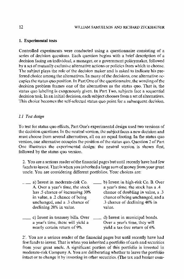
To test for status quo effects, Part One’s experimental design used two versions of the decision questions. In the neutral version, the subject faces a new decision and must choose from several alternatives, all on an equal footing. In the status quo version, one alternative occupies the position of the status quo. Question 2 of Part One illustrates the experimental design: the neutral version is shown first, followed by the status quo version.
2. You are a serious reader of the financial pages but until recently have had few funds to invest. That is when you inherited a large sum of money from your great uncle. You are considering different portfolios. Your choices are:
__ a) Invest in moderate-risk Co. - b) Invest in high-risk Co. B. Over A. Over a year’s time, the stock a year’s time, the stock has a .4 has .5 chance of increasing 30% chance of doubling in value, a .3 in value, a .2 chance of being chance of being unchanged, and a unchanged, and a .3 chance of .3 chance of declining 40% in declining 20% in value. value.
__ c) Invest in treasury bills. Over __ d) Invest in municipal bonds. a year’s time, these will yield a Over a year’s time, they will nearly certain return of 9%. yield a tax-free return of 6%.
2’. You are a serious reader of the financial pages but until recently have had few funds to invest. That is when you inherited a portfolio of cash and securities from your great uncle. A significant portion of this portfolio is invested in moderate-risk Company A. You are deliberating whether to leave the portfolio intact or to change it by investing in other securities. (The tax and broker com-
STATUS QUO BIAS IN DECISION h4AKING 13
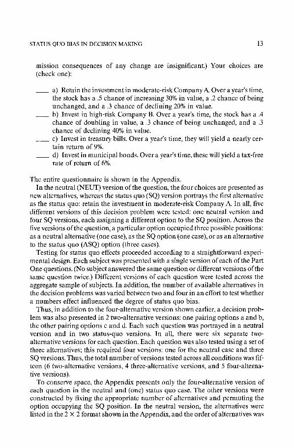
mission consequences of any change are insignificant.) Your choices are (check one):
__ a) Retain the investment in moderate-risk Company A. Over a year’s time, the stock has a .5 chance of increasing 30% in value, a .2 chance of being unchanged, and a .3 chance of declining 20% in value.
__ b) Invest in high-risk Company B. Over a year’s time, the stock has a .4 chance of doubling in value, a .3 chance of being unchanged, and a .3 chance of declining 40% in value.
- c) Invest in treasury bills. Over a year’s time, they will yield a nearly cer- tain return of 9%.
- d) Invest in municipal bonds. Over a year’s time, these will yield a tax-free rate of return of 6%.
The entire questionnaire is shown in the Appendix. In the neutral (NEUT) version of the question, the four choices are presented as
new alternatives, whereas the status quo (SQ) version portrays the first alternative as the status quo: retain the investment in moderate-risk Company A. In all, five different versions of this decision problem were tested: one neutral version and four SQ versions, each assigning a different option to the SQ position. Across the five versions of the question, a particular option occupied three possible positions: as a neutral alternative (one case), as the SQ option (one case), or as an alternative to the status quo (ASQ) option (three cases).
Testing for status quo effects proceeded according to a straightforward experi- mental design. Each subject was presented with a single version of each of the Part One questions. (No subject answered the same question or different versions of the same question twice.) Different versions of each question were tested across the aggregate sample of subjects. In addition, the number of available alternatives in the decision problems was varied between two and four in an effort to test whether a numbers effect influenced the degree of status quo bias.
Thus, in addition to the four-alternative version shown earlier, a decision prob- lem was also presented in 2 two-alternative versions: one pairing options a and b, the other pairing options c and d. Each such question was portrayed in a neutral version and in two status-quo versions. In all, there were six separate two- alternative versions for each question. Each question was also tested using a set of three alternatives; this required four versions: one for the neutral case and three SQ versions. Thus, the total number of versions tested across all conditions was fif- teen (6 two-alternative versions, 4 three-alternative versions, and 5 four-alterna- tive versions).
To conserve space, the Appendix presents only the four-alternative version of each question in the neutral and (one) status quo case. The other versions were constructed by fixing the appropriate number of alternatives and permuting the option occupying the SQ position. In the neutral version, the alternatives were listed in the 2 X 2 format shown in the Appendix, and the order of alternatives was
14 WILLIAM SAMUELSON AND RICHARD ZECKHAUSER
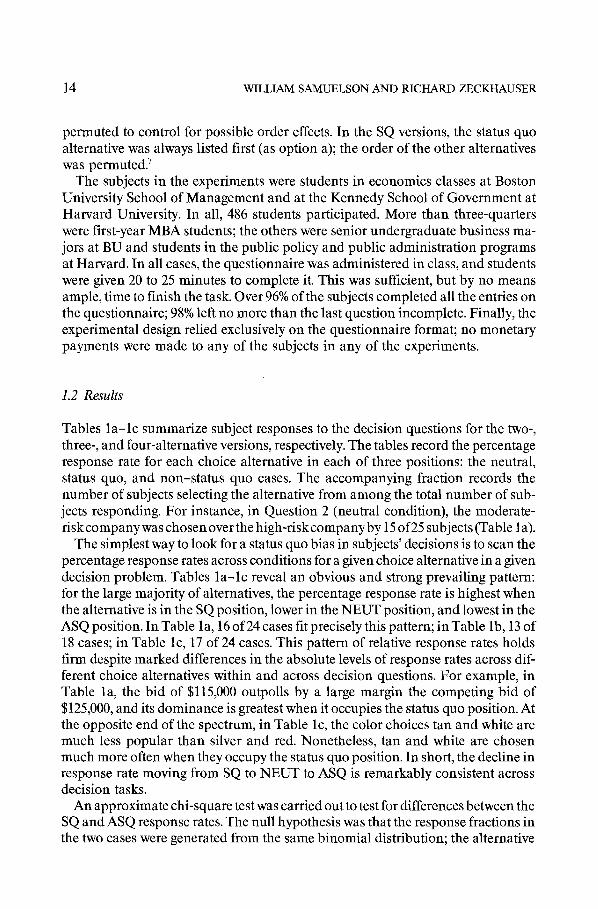
permuted to control for possible order effects. In the SQ versions, the status quo alternative was always listed first (as option a); the order of the other alternatives was permuted.7
The subjects in the experiments were students in economics classes at Boston University School of Management and at the Kennedy School of Government at Harvard University. In all, 486 students participated. More than three-quarters were first-year MBA students; the others were senior undergraduate business ma- jors at BU and students in the public policy and public administration programs at Harvard. In all cases, the questionnaire was administered in class, and students were given 20 to 25 minutes to complete it. This was sufficient, but by no means ample, time to finish the task. Over 96% of the subjects completed all the entries on the questionnaire; 98% left no more than the last question incomplete. Finally, the experimental design relied exclusively on the questionnaire format; no monetary payments were made to any of the subjects in any of the experiments.
1.2 Results
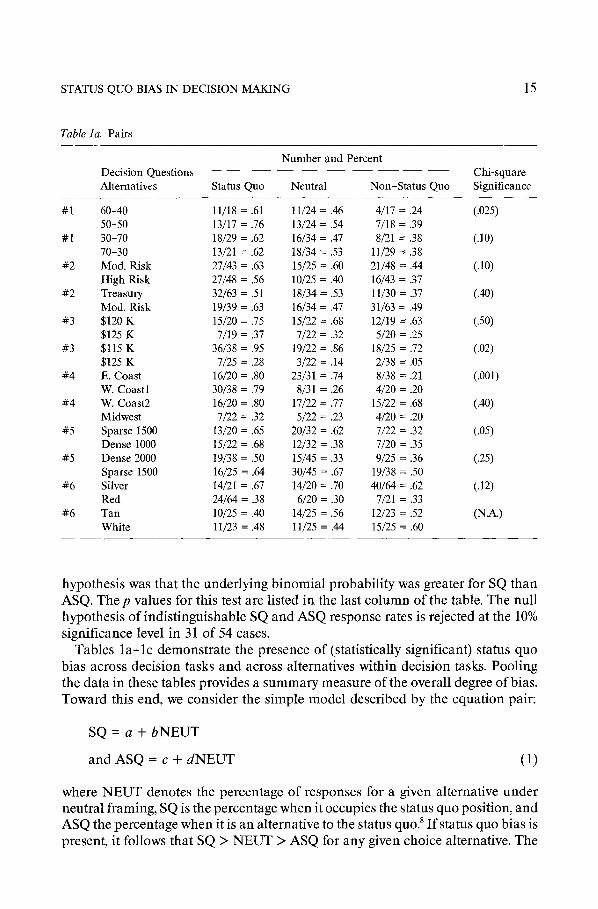
Tables la-lc summarize subject responses to the decision questions for the two-, three-, and four-alternative versions, respectively. The tables record the percentage response rate for each choice alternative in each of three positions: the neutral, status quo, and non-status quo cases. The accompanying fraction records the number of subjects selecting the alternative from among the total number of sub- jects responding. For instance, in Question 2 (neutral condition), the moderate- riskcompanywas chosenoverthe high-riskcompany by 15 of25 subjects (Table la).
The simplest way to look for a status quo bias in subjects’ decisions is to scan the percentage response rates across conditions for a given choice alternative in a given decision problem. Tables la-lc reveal an obvious and strong prevailing pattern: for the large majority of alternatives, the percentage response rate is highest when the alternative is in the SQ position, lower in the NEUT position, and lowest in the ASQ position. In Table la, 16 of 24 cases fit precisely this pattern; in Table lb, 13 of 18 cases; in Table lc, 17 of 24 cases. This pattern of relative response rates holds firm despite marked differences in the absolute levels of response rates across dif- ferent choice alternatives within and across decision questions. For example, in Table la, the bid of $115,000 outpolls by a large margin the competing bid of $125,000, and its dominance is greatest when it occupies the status quo position. At the opposite end of the spectrum, in Table lc, the color choices tan and white are much less popular than silver and red. Nonetheless, tan and white are chosen much more often when they occupy the status quo position. In short, the decline in response rate moving from SQ to NEUT to ASQ is remarkably consistent across decision tasks.
An approximate chi-square test was carried out to test for differences between the SQ and ASQ response rates. The null hypothesis was that the response fractions in the two cases were generated from the same binomial distribution; the alternative
STATUS QUO BIAS IN DECISION MAKING 15
Table la. Pairs
Decision Questions Alternatives
Number and Percent Chi-square
Status Quo Neutral Non-Status Quo Significance
#l
#I
#2
#2
#3
#3
#4
#4
#5
#5
#6
#6
60-40 50-50 30-70 70-30 Mod. Risk High Risk Treasury Mod. Risk $120 K $125 K $115 K $125 K E. Coast W. Coast1 W. Coast2 Midwest Sparse 1500 Dense 1000 Dense 2000 Sparse 1500 Silver Red Tan White
11/18 = .61 13117 = .76 18/29 = .62 13/21 = .62 21143 = .63 27148 = .56 32/63 = .51 19139 = .63 15/20 = .75
7/19 = .37 36138 = .95
7125 = .28 16/20 = .80 30/38 = .I9 16/20 = 230
7/22 = .32 13120 = .65 15122 = .68 19/38 = .50 16125 = .64 14121 = .67 24164 = .38 10125 = .40 11/23 = .48
11124 = .46 13124 = .54 16134 = .41 18134 = .53 15/25 = .60 lo/25 = .40 18134 = .53 16134 = .47 15122 = .68 7122 = .32
19122 = .86 3122 = .14
23131 = .74 8131 = .26
Ill22 = .77 5122 = .23
20132 = .62 12132 = .38 15145 = .33 30145 = .67 14/20 = .70
6120 = .30 14125 = .56 11125 = .44
4117 = .24 II18 = .39 8121 = .38
11129 = .38 21148 = .44 16143 = .37 11/30 = .37 31163 = .49 12119 = .63
5120 = .25 18125 = .I2
2138 = .OS 8f38 = .21 4f20 = .20
15122 = .68 4120 = .20 7122 = .32 7120 = .35 9125 = .36
19/38 = .50 40164 = .62
7121 = .33 12123 = .52 15125 = .60
(.025)
(JO)
(JO)
(.40)
(.50)
W)
(.OOl)
(.40)
(.05)
(.25)
w
(N.-w
hypothesis was that the underlying binomial probability was greater for SQ than ASQ. Thep values for this test are listed in the last column of the table. The null hypothesis of indistinguishable SQ and ASQ response rates is rejected at the 10% significance level in 31 of 54 cases.
Tables la-lc demonstrate the presence of (statistically significant) status quo bias across decision tasks and across alternatives within decision tasks. Pooling the data in these tables provides a summary measure of the overall degree of bias. Toward this end, we consider the simple model described by the equation pair:
SQ=a+bNEUT
and ASQ = c + dNEUT (1)
where NEUT denotes the percentage of responses for a given alternative under neutral framing, SQ is the percentage when it occupies the status quo position, and ASQ the percentage when it is an alternative to the status quo.8 If status quo bias is present, it follows that SQ > NEUT > ASQ for any given choice alternative. The
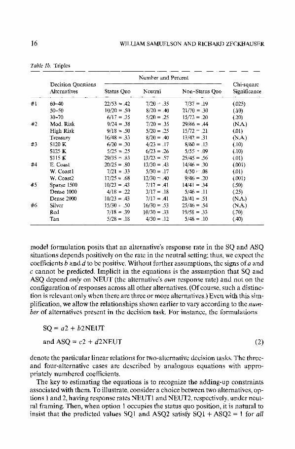
16 WILLIAM SAMUELSON AND RICHARD ZECKHAUSER
Table lb. Triples
Decision Questions Number and Percent
Chi-square
#l
#2
#3
#4
#5
#6
Alternatives Status Quo
60-40 22153 = .42 50-50 10/20 = .50 30-70 6117 = .35 Mod. Risk 9124 = .38 High Risk 9/18 = .50 Treasury 16/48 = .33 $120 K 6120 = .30 $125 K 5125 = .25 $115 K 29135 = .83 E. Coast 20125 = .80 W. Coast1 7121 = .33 W. Coast2 17125 = .68 Sparse 1500 10123 = .43 Dense 1000 4/18 = .22 Dense 2000 lo/23 = .43 Silver 15130 = .50 Red 7118 = .39 Tan 5/28 = .18
Neutral
7120 = .35 8/20 = 40 5120 = .25 7120 = .35 5120 = .25 8/20 = .40 4123 = .17 6123 = .26
13123 = .57 13/30 = .43 5130 = .17
12130 = .40 7117 = .41 3/17 = .18 7117 = .41
16130 = .53 10/30 = .33
4130 = .I2
Non-Status Quo
7137 = .19
21170 = .30 15173 = .20 29166 = .44 15172 = .21 13142 = .31 8160 = .13 5155 = .09
25145 = .56 14/46 = .30
4150 = .08 9146 = .20
14141 = .34 5146 = .ll
21/41 = .51 25146 = .54 19/58 = .33
5/48 = .lO
Significance
(.025)
cw c-w O\J.N co11 WA.1 (.W UO) cw (.OOl)
cw (.OOl)
(.50) (.25) WA.) WA) (.70) (.40)
model formulation posits that an alternative’s response rate in the SQ and ASQ situations depends positively on the rate in the neutral setting; thus, we expect the coefficients b and d to be positive. Without further assumptions, the signs of a and c cannot be predicted. Implicit in the equations is the assumption that SQ and ASQ depend on2y on NEUT (the alternative’s owlz response rate) and not on the configuration of responses across all other alternatives. (Of course, such a distinc- tion is relevant only when there are three or more alternatives.) Even with this sim- plification, we allow the relationships shown earlier to vary according to the num- ber of alternatives present in the decision task. For instance, the formulations
SQ = a2 + b2NEUT
and ASQ = c2 + d2NEUT (2)
denote the particular linear relations for two-alternative decision tasks. The three- and four-alternative cases are described by analogous equations with appro- priately numbered coefficients.
The key to estimating the equations is to recognize the adding-up constraints associated with them. To illustrate, consider a choice between two alternatives, op- tions 1 and 2, having response rates NEUTl and NEUT2, respectively, under neut- ral framing. Then, when option 1 occupies the status quo position, it is natural to insist that the predicted values SQl and ASQ2 satisfy SQl + ASQ2 = 1 for all

STATUS QUO BIAS IN DECISION MAKING
Table Ic. Quads
Number and Percent Decision Questions Alternatives Status Quo Neutral Non-Status Quo
17
Chi-square Significance
#l
#2
#3
#4
#5
#6
60-40 SO-50 30-70 70-30 Mod. Risk High Risk Treasury Municipal $120 K $125 K $115 K $130 K E. Coast W. Coast1 W. Coast2 Midwest Sparse 1500 Dense 1000 Dense 2000 Sparse 1500 Silver Red Tan White
7119 = .37 12137 = .32 13124 = .54 25148 = .52
7118 = .39 8129 = 28
13145 = .29 9119 = .41
20162 = .32 13/50 = .26 41154 = .76
3128 = .11 13120 = 65 3125 = .12
19/29 = .66 9160 = .15
12119 = .63 4124 = .17
10129 = .34 6120 = .30
32/42 = .I6 24145 = .53
S/38 = .13 15154 = .28
6128 = .21 6f28 = .21
11/28 = .39 5/28 = .18 9128 = .32 5128 = .18 5/28 = .18 9128 = .32 5/31 = .I6 6131 = .19
18/31 = .58 2131 = .06
24146 = .52 l/46 = .02
18/46 = .39 3146 = .07 9122 = .41 2122 = 39 6122 = .21 5122 = .23
12123 = .52 5123 = .22 2123 = .09 4/23 = .17
7/109 = .06 22191 =.24
29/104 = .28 13/80 =.16 21193 = .29 17/82 = .21 11166 = .17 19192 = .21
281122 = .23 20/142 = .14 631140 = .45
6/166 = .04 33/114 = .29
9/109 = .08 42/105 = .40
7174 = .09 25173 = .34
2168 = .03 21163 = .33 12/72 = .17
681137 = .50 20/134 = .I5
3/141 = .02 1 l/125 = .09
(.OOl) C35) (.W (.OOl) (.40) C50) (.15) w4 W) (.05) (.OOl) C.10) (.005)
(.W W) (.30) (.025)
CO2) (.95) (W (.OOS) (.OOl) (.05) (.OOl)
NEUTl and NEUT2 such that NEUTl + NEUT2 = 1. But this requirement is satisfied if and only if b2 = d2 and a2 + c2 + d2 = 1. This is shown by simply ad- ding the equations and making a substitution to obtain
SQl + ASQ2 = (a2 + c2 + d2) + (b2 - d2)NEUTl (3)
Since the left-hand side must sum to unity, so too must the right (for any value of NEUTl), implying the coefficient restrictions listed earlier. The analogous restric- tions for the three- and four-alternative cases are
b3 = d3, a3 + 2~3 + d3 = 1 and b4 = d4, a4 + 3~4 + d4 = 1 (4)
Besides the intercept restrictions, the important constraint is that the equations for SQ and ASQ have equal slopes?
We used the pooled data in Tables la- lc to estimate the coefficients in the linear model subject to the coefficient restrictions noted earlier. Under the working hypothesis that variations in SQ and ASQ (unaccounted for by NEUT) were ran-
18 WILLIAM SAMUELSON AND RICHARD ZECKHAUSER
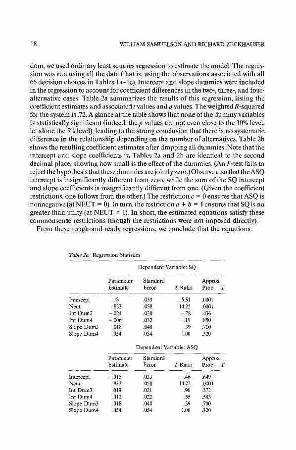
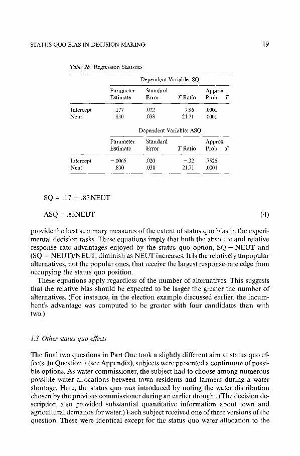
dom, we used ordinary least squares regression to estimate the model. The regres- sion was run using all the data (that is, using the observations associated with all 66 decision choices in Tables la-lc). Intercept and slope dummies were included in the regression to account for coefficient differences in the two-, three-, and four- alternative cases. Table 2a summarizes the results of this regression, listing the coefficient estimates and associated t values andp values. The weightedR-squared for the system is .72. A glance at the table shows that none of the dummy variables is statistically significant (indeed, the p values are not even close to the 10% level, let alone the 5% level), leading to the strong conclusion that there is no systematic difference in the relationship depending on the number of alternatives. Table 2b shows the resulting coefficient estimates after dropping all dummies. Note that the intercept and slope coefficients in Tables 2a and 2b are identical to the second decimal place, showing how small is the effect of the dummies. (An F-test fails to reject the hypothesis that these dummies are jointly zero.) Observe also that the ASQ intercept is insignificantly different from zero, while the sum of the SQ intercept and slope coefficients is insignificantly different from one. (Given the coefficient restrictions, one follows from the other.) The restriction c = 0 ensures that ASQ is nonnegative (at NEUT = 0). In mm, the restriction a + b = 1 ensures that SQ is no greater than unity (at NEUT = 1). In short, the estimated equations satisfy these commonsense restrictions (though the restrictions were not imposed directly).
From these rough-and-ready regressions, we conclude that the equations
Table 2a. Regression Statistics
Dependent Variable: SQ
Parameter Estimate
Standard Error
Approx 7’ Ratio Prob T
Intercept .18 ,033 5.51 .OOOl Neut .833 ,058 14.22 .OOOl Int Dum3 -.024 ,030 -.78 ,436 Int Dum4 -.006 .032 -.19 ,850 Slope Dum3 ,018 ,048 .39 .700 Slope Dum4 ,054 ,054 1.00 .320
Dependent Variable: ASQ
Parameter Standard Estimate Error T Ratio
Approx Prob T
Intercept -.015 ,033 -.46 .649 Neut ,833 .058 14.22 .OOOl Int Dum3 ,019 ,021 .90 ,312 Int Dum4 .012 ,022 .55 ,583 Slope Dum3 ,018 ,048 .39 .700 Slope Dum4 ,054 ,054 1.00 ,320
STATUS QUO BIAS IN DECISION MAKING 19
Table 2b. Regression Statistics
Dependent Variable: SQ
Parameter Standard Approx Estimate Error T Ratio Prob T
Intercept ,177 ,022 1.96 .OOOl Neut ,830 ,038 21.71 .Oool
Intercept Neut
Dependent Variable: ASQ
Parameter Standard Approx Estimate Error T Ratio Prob T
-.0065 .020 -.32 .I525 ,830 .038 21.71 .OOOl
SQ = .17 + .83NEUT
ASQ = .83NEUT (4)
provide the best summary measures of the extent of status quo bias in the experi- mental decision tasks. These equations imply that both the absolute and relative response rate advantages enjoyed by the status quo option, SQ - NEUT and (SQ - NEUT)/NEUT, diminish as NEUT increases. It is the relatively unpopular alternatives, not the popular ones, that receive the largest response-rate edge from occupying the status quo position.
These equations apply regardless of the number of alternatives. This suggests that the relative bias should be expected to be larger the greater the number of alternatives. (For instance, in the election example discussed earlier, the incum- bent’s advantage was computed to be greater with four candidates than with two.)
1.3 Other status quo effects
The final two questions in Part One took a slightly different aim at status quo ef- fects. In Question 7 (see Appendix), subjects were presented a continuum of possi- ble options. As water commissioner, the subject had to choose among numerous possible water allocations between town residents and farmers during a water shortage. Here, the status quo was introduced by noting the water distribution chosen by the previous commissioner during an earlier drought. (The decision de- scription also provided substantial quantitative information about town and agricultural demands for water.) Each subject received one of three versions of the question. These were identical except for the status quo water allocation to the

20 WILLIAM SAMUELSON AND RICHARD ZECKHAUSER
town, which was either 100,000,200,000, or 300,000 acre-feet. We sought to isolate the impact of status quo anchoring (relative to the influence of other sources of in- formation) by comparing response results across the three versions. Our working hypothesis was that, other things equal, the greater the status quo allocation to the town, the greater would be the actual allocation.
Table 3, which lists the distribution of responses by version, strongly bears out this hypothesis. Starting from a 100,000 acre-feet SQ allocation and proceeding to larger ones, each subsequent distribution of responses stochastically dominates (i.e., can be formed by rightward shifts in) its predecessor. A chi-square test strongly rejects the hypothesis that the responses across versions are drawn from the same multinomial distribution. A simple way to gauge the impact of the SQ is to compare the mean allocations across the versions. These are 153,000, 183,000, and 200,000 in order of ascending SQ allocations. The influence of the SQ alloca- tion is obvious. Note, however, that subject decisions are only partially anchored to the status quo point; that is, they are moved by other factors as well. Thus, a 200,000 (i.e., 300,000 - 100,000) difference in the SQ allocation implies roughly a 50,000 acre-foot impact on the chosen allocation.
Question 8 measures the value consequences of status quo bias. As chief of a consulting firm, subjects were asked to report their willingness to pay to relocate their office quarters from an older to a newer (more conveniently located) build- ing. In a second version, all information was the same except that the company’s present quarters were in the newer building and the proposed move was to the older building. In either case, the description stated that as an inducement the company’s moving costs and other expenses would be paid by the landlord-to-be. Compensating values were expressed as a percentage of the current rental rate (which was left unspecified). Letx denote the percentage rent increase the subject would be just willing to pay for a move from old to new;y denotes the required rent
Table 3. Water Allocations
a) 100,000 a-f (60 subjects)
Status Quo Allocation b) 200,000 a-f
(67 subjects) c) 300,000 a-f
(61 subjects)
Town Allocation chosen by subjects Percentage of Responses
50,000 3 1 2 100,000 21 4 5 150,000 52 30 21 200,000 17 48 46 250,000 5 12 20 300,000 2 5 6
Total 100 100 100
STATUS QUO BIAS IN DECISION MAKING 21
percentage reduction for a move from new to old. If the subjects show no bias in evaluating the move, these values should be the same when expressed relative to the same base: y = x/(1 + x). That is, for bias-free subjects, y should be nearly equal to (but slightly less than) X. On the other hand, if status quo bias is signifi- cant, one would expecty > x, reflecting a preference for the status quo (regardless of what the status quo is). Thus, the subject would insist on a large rent reduction to induce a move from new to old but would tolerate only a small rent increase for a move in the opposite direction.
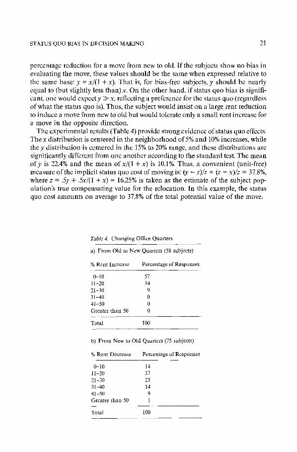
The experimental results (Table 4) provide strong evidence of status quo effects. The x distribution is centered in the neighborhood of 5% and 10% increases, while the y distribution is centered in the 15% to 20% range, and these distributions are significantly different from one another according to the standard test. The mean of y is 22.4% and the mean of x/(1 + X) is 10.1%. Thus, a convenient (unit-free) measure of the implicit status quo cost of moving is: Cy - z)/z = (z - x)/z = 37.8%, where z = .5y -I- .5x/(1 + x) = 16.25% is taken as the estimate of the subject pop- ulation’s true compensating value for the relocation. In this example, the status quo cost amounts on average to 37.8% of the total potential value of the move.
Table 4. Changing Office Quarters
a) From Old to New Quarters (58 subjects)
% Rent Increase Percentage of Responses
O-10 51 11-20 34 21-30 9 31-40 0 41-50 0 Greater than 50 0
Total 100
b) From New to Old Quarters (75 subjects)
% Rent Decrease Percentage of Responses
O-10 14 11-20 37 21-30 25 31-40 14 41-50 9 Greater than 50 1
Total 100
22 WILLIAM SAMUELSON AND RICHARD ZECKHAUSER
1.4 Sequential decisions
Subject responses in Part One of the questionnaire provide a strong demonstra- tion of individual decision bias in the case of an exogenously determined status quo. Part Two sought to test whether a similar bias occurs when subjects self-select their own status quo options. The Appendix reproduces the decision problem (Part Two, 1) that was used for this purpose. It can be summarized as follows. As a member of top management of a regional airline, the subject was asked to decide the number and type of aircraft to lease in each of two years. There was no cost to switching leases between the two years. Because the airline must commit to its lease decision a year in advance, it will be uncertain about economic conditions over the lease period, though it has limited information (economic forecasts) about these conditions. For each year, subjects received one of two forecasts: good conditions (high demand and stable air fares) or bad conditions (lower demand and price wars).
To test for status quo effects, we compared results across two versions of the questionnaire differing with respect to the order of the economic conditions. In one version, the subject received forecasts of good conditions in year one (first deci- sion). After making a decision (and passing in his or her questionnaire sheet), he or she received a second sheet requesting his or her lease decision for year two, this time under bad conditions. In the other version, the order of economic conditions was reversed: the subject received a bad forecast for the year one decision and a good forecast for year two.
Consider the first version: a good forecast followed by a bad one. Subjects would presumably tend to lease large fleets in year one (under good conditions). As a result, when it comes to the second decision, a large fleet will occupy the status quo position. Given a forecast of bad conditions, the airline should choose to lease a small fleet. However, this inclination will be reduced by any status quo inertia. To be more specific, if a status quo bias exists, one would observe lager fleets under bad conditions in year two (after good conditions) than in year one under bad con- ditions. Similarly, one would observe smaller fleets under good conditions in year two (following bad conditions) than in year one under good conditions. To sum up, status quo bias would be manifested in an anchoring effect-second-year deci- sions would be anchored in part to first-year decisions. By changing the order of the economic conditions, we manipulate the position of the anchor.
The results of Part Two are displayed in Tables 5 through 8. Table 5 depicts a se- quential decision involving binary choices: a small fleet (six loo-seat aircraft and no 150-seat aircraft: 6-O) or a large (6-4) fleet in year one with the same choice alter- natives repeated in year two. The table lists the number and percentage of re- sponses associated with each of the possible sequential decisions. For instance, in Table 5a, 50% of the subjects chose six loo-seat aircraft and four 150-seat aircraft in year one under good conditions and held to this choice in year two under bad con- ditions. The percentages represent joint probabilities (not conditional prob- abilities) and thus sum to 100% across the table. Marginal probabilities are shown in the row and column margins.

STATUS QUO BIAS IN DECISION MAKING 23
Table 5. Leasing an Air Fleet (Version 1)
a) Good then Bad (28 subjects)
Year One (Good Conditions)
Year Two (Bad Conditions)
6-O 6-4 Total
6-O 29% 7% 36% 6-4 14% 50% 64%
Total 43% 57% 100%
b) Bad then Good (23 subjects)
Year One (Bad Conditions)
Year Two (Good Conditions)
6-O 6-4 Total
6-O 43% 14% 57% 6-4 0% 43% 43%
Total 43% 57% 100%
The results in Table 5 are consistent with the expected qualitative effects. In year one, a large fleet was the majority choice under good conditions and the minority choice under bad conditions. Between years one and two, there was a significant extent of status quo inertia-79% (.29 + .50) of the subjects retained their previous choice in Table 5a, 86% (.43 + .43) in Table 5b. We emphasize, however, that status quo inertia is not itself evidence of status quo bias. It is perfectly possible that some subjects prefer the 6-O fleet (or the 6-4 fleet) under any economic conditions. A test of status quo bias requires a comparison of the appropriate marginal probabilities. Let Pr(6-41G) denote the percentage of subjects making this fleet choice in year one under good conditions. Similarly, let Pr(6-4jG after B) denote the percentage in year two under good conditions after bad conditions in year one. From the table, these probabilities are Pr(6-41G) = 64 and Pr(6-41G after B) = .57. These percentages are consistent with a status quo bias: the prior year’s bad conditions induce smaller fleets not only then but also during the next year, other things (good conditions) equal. Though in the expected direction, the difference in pro- babilities is not statistically significant. (The chi-square test with respect to the hypothesis of no difference has a p value of .60.) In addition, we find that Pr(6-4lB) = .43 and Pr(6-4lB after G) = .57. Again thte ranking of probabilities is consistent with status quo anchoring. However, the relation still falls short of the 10% significance level; the p value is .35.
The results of a second version of the sequential decision are listed in Tables 6 and 7. Here, with four alternatives available in the second decision, we hypothe- sized that, for reasons of bounded rationality, status quo effects might be stronger

24 WILLIAM SAMUELSON AND RICHARD ZECKHAUSER
Table 6. Leasing an Air Fleet (Version 2)
a) Good then Bad (39 subjects)
Year One (Good Conditions) o-4
Year Two (Bad Conditions)
6-O 6-4 6-4A Total
6-O 6-4
Total
0% 18% 3% 5% 26% 20% 13% 0% 41% 74%
20% 31% 3% 46% 100%
b) Bad then Good (56 subjects)
Year One (Good Conditions) o-4
Year Two (Bad Conditions)
6-O 6-4 6-4A Total
6-O 13% 33% 3% 18% 66% 6-4 14% 3% 0% 16% 34%
Total 27% 36% 3% 34% 100%
Table 7. Leasing an Air Fleet (Version 3)
a) Good then Bad (19 subjects)
Year One (Good Conditions)
o-4 6-4A
o-4
21% 0%
Year Two (Bad Conditions)
6-O 6-4 6-4A Total
16% 0% 5% 42% 5% 10% 43% 58%
Total 21% 21% 10% 48% 100%
b) Bad then Good (29 subjects)
Year One (Bad Conditions) o-4
Year Two (Good Conditions)
6-O 6-4 6-4A Total
o-4 21% 3% 3% 7% 34% 6-4A 0% 7% 7% 52% 66%
Total 21% 10% 10% 59% 100%
STATUS QUO BIAS IN DECISION MAKING 25
Table 8. Leasing an Air Fleet (Version 4)
a) Good then Bad (75 subjects)
Year Two (Bad Conditions) Year One (Good Conditions) o-4 l-4 6-3 6-4 Total
o-4 5% 5% 3% 0% 13% 6-4 1% 10% 32% 44% 87%
Total 6% 15% 35% 44% 100%
b) Bad then Good (50 subjects)
Year One (Bad Conditions) o-4
Year Two (Good Conditions)
l-4 6-3 6-4 Total
o-4 14% 14% 10% 0% 38% 6-4 0% 6% 22% 34% 62%
Total 14% 20% 32% 34% 100%
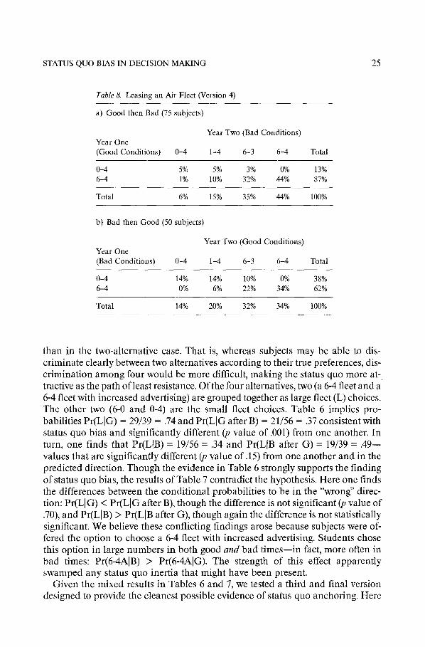
than in the two-alternative case. That is, whereas subjects may be able to dis- criminate clearly between two alternatives according to their true preferences, dis- crimination among four would be more difficult, making the status quo more at- tractive as the path of least resistance. Of the four alternatives, two (a 6-4 fleet and a 6-4 fleet with increased advertising) are grouped together as large fleet (L) choices. The other two (6-O and O-4) are the small fleet choices. Table 6 implies pro- babilities Pr(LIG) = 29/39 = .74 and Pr(LIG after B) = 21/56 = .37 consistent with status quo bias and significantly different (p value of .OOl) from one another. In turn, one finds that Pr(L1B) = 19/56 = .34 and Pr(LIB after G) = 19/39 = .49- values that are significantly different (p value of .15) from one another and in the predicted direction. Though the evidence in Table 6 strongly supports the finding of status quo bias, the results of Table 7 contradict the hypothesis. Here one finds the differences between the conditional probabilities to be in the “wrong” direc- tion: Pr(LI G) < Pr(LI G after B), though the difference is not significant @ value of .70), and Pr(LIB) > Pr(LIB after G), though again the difference is not statistically significant. We believe these conflicting findings arose because subjects were of- fered the option to choose a 6-4 fleet with increased advertising. Students chose this option in large numbers in both good and bad times-in fact, more often in bad times: Pr(6-4AlB) > Pr(6-4AIG). The strength of this effect apparently swamped any status quo inertia that might have been present.
Given the mixed results in Tables 6 and 7, we tested a third and final version designed to provide the cleanest possible evidence of status quo anchoring. Here
26 WILLIAM SAMUELSON AND RICHARD ZECKHAUSER
the initial alternatives were fleets of O-4 and 6-4, and the second-period alternatives were O-4, l-4,6-3, and 6-4. The results in Table 8 provide the strongest evidence of status quo anchoring. In year one, 87% of subjects chose the large fleet under good conditions. Under bad conditions in the following year, the vast majority of these same subjects retained a large fleet. Not all were anchored fast to 6-4; almost half the group dragged the anchor slightly and settled on 6-3. Similarly, under bad con- ditions in year one, a sizeable minority chose O-4 and then retained a small fleet (either O-4 or l-4) in year two when conditions were good. A comparison of the conditional probabilities shows that Pr(L(G) = 65/75 = 87, and this is signifi- cantly greater (p value of .Ol) than Pr(LIG after B) = 33/50 = .66. In turn, one finds that Pr(LIB) = 3 l/50 = .62, and this is significantly less (p value of .05) than Pr(LIB after G) = 59/75 = .79.
Taking together the results of Tables 5 and 7 (which fail the test of significance) and Tables 6 and 8 (which find statistically significant anchoring effects), we con- clude that the sequential decision tasks show some evidence of status quo bias, most prominently in cases that involve many alternatives.”
2. Field studies
Many people make the same choices year after year in important periodic decisions. It is the rare individual who fine-tunes such choices to changing economic circumstances, even though the transition costs may be small and the importance great. This section examines the incidence of status quo inertia in two kinds of periodic decisions: individual health plan choices and contributions to retirement funds.
2.1 Harvard University health plans
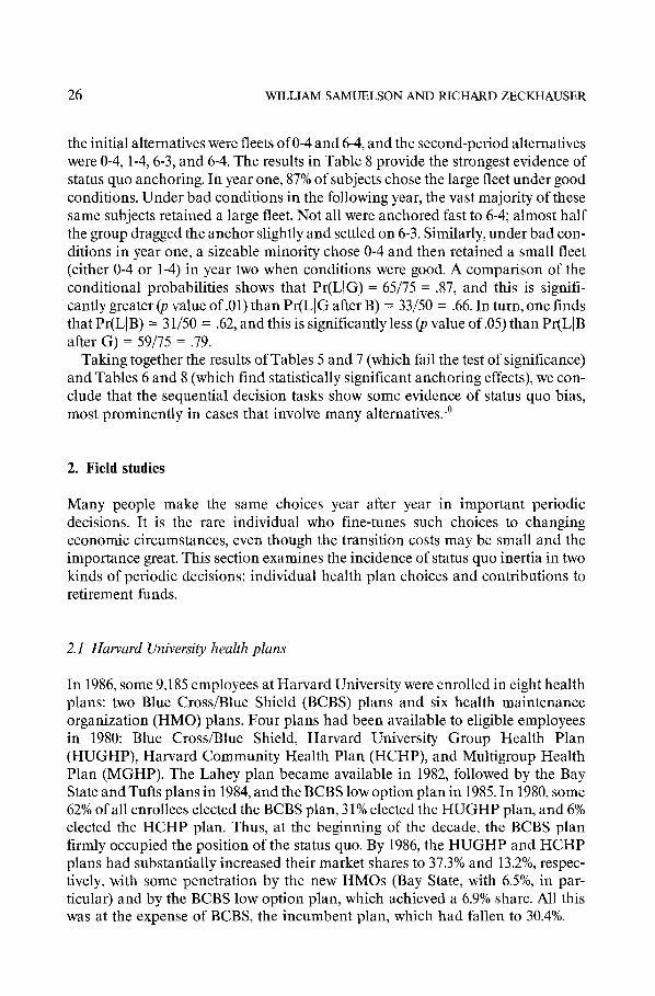
In 1986, some 9,185 employees at Harvard University were enrolled in eight health plans: two Blue Cross/Blue Shield (BCBS) plans and six health maintenance organization (HMO) plans. Four plans had been available to eligible employees in 1980: Blue Cross/Blue Shield, Harvard University Group Health Plan (HUGHP), Harvard Community Health Plan (HCHP), and Multigroup Health Plan (MGHP). The Lahey plan became available in 1982, followed by the Bay State and Tufts plans in 1984, and the BCBS low option plan in 1985. In 1980, some 62% of all enrollees elected the BCBS plan, 3 1% elected the HUGHP plan, and 6% elected the HCHP plan. Thus, at the beginning of the decade, the BCBS plan firmly occupied the position of the status quo. By 1986, the HUGHP and HCHP plans had substantially increased their market shares to 37.3% and 13.2%, respec- tively, with some penetration by the new HMOs (Bay State, with 6.5%, in par- ticular) and by the BCBS low option plan, which achieved a 6.9% share. All this was at the expense of BCBS, the incumbent plan, which had fallen to 30.4%.
STATUS QUO BIAS IN DECISION MAKING 27
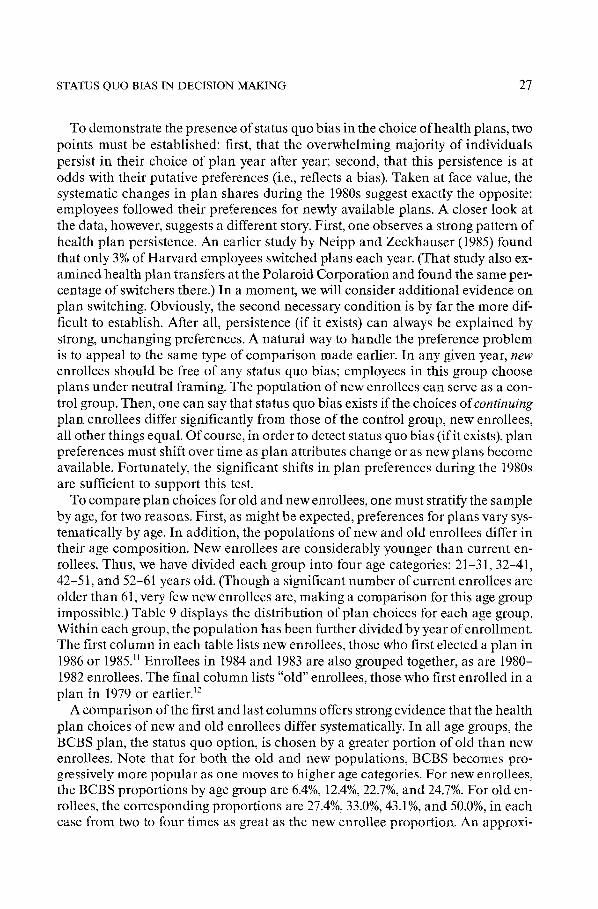
To demonstrate the presence of status quo bias in the choice of health plans, two points must be established: first, that the overwhelming majority of individuals persist in their choice of plan year after year; second, that this persistence is at odds with their putative preferences (i.e., reflects a bias). Taken at face value, the systematic changes in plan shares during the 1980s suggest exactly the opposite: employees followed their preferences for newly available plans. A closer look at the data, however, suggests a different story. First, one observes a strong pattern of health plan persistence. An earlier study by Neipp and Zeckhauser (1985) found that only 3% of Harvard employees switched plans each year. (That study also ex- amined health plan transfers at the Polaroid Corporation and found the same per- centage of switchers there.) In a moment, we will consider additional evidence on plan switching. Obviously, the second necessary condition is by far the more dif- ficult to establish. After all, persistence (if it exists) can always be explained by strong, unchanging preferences. A natural way to handle the preference problem is to appeal to the same type of comparison made earlier. In any given year, new enrollees should be free of any status quo bias; employees in this group choose plans under neutral framing. The population of new enrollees can serve as a con- trol group. Then, one can say that status quo bias exists if the choices of continuing plan enrollees differ significantly from those of the control group, new enrollees, all other things equal. Of course, in order to detect status quo bias (if it exists), plan preferences must shift over time as plan attributes change or as new plans become available. Fortunately, the significant shifts in plan preferences during the 1980s are sufficient to support this test.
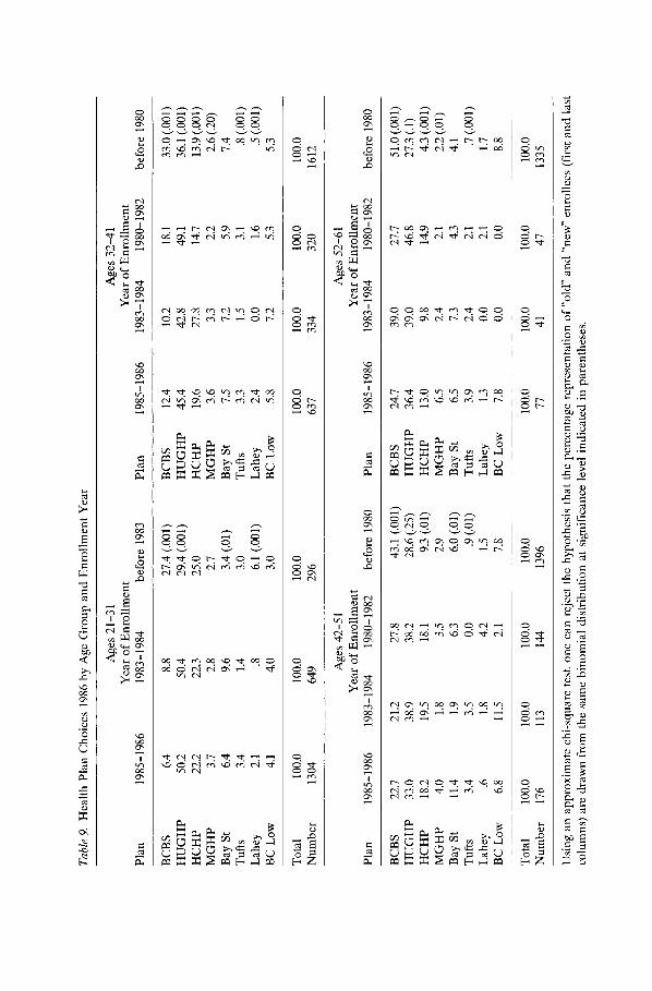
To compare plan choices for old and new enrollees, one must stratify the sample by age, for two reasons. First, as might be expected, preferences for plans vary sys- tematically by age. In addition, the populations of new and old enrollees differ in their age composition. New enrollees are considerably younger than current en- rollees. Thus, we have divided each group into four age categories: 21-31, 32-41, 42-51, and 52-61 years old. (Though a significant number of current enrollees are older than 61, very few new enrollees are, making a comparison for this age group impossible.) Table 9 displays the distribution of plan choices for each age group. Within each group, the population has been further divided by year of enrollment. The first column in each table lists new enrollees, those who first elected a plan in 1986 or 1985.” Enrollees in 1984 and 1983 are also grouped together, as are 1980- 1982 enrollees. The final column lists “old” enrollees, those who first enrolled in a plan in 1979 or earlier.”
A comparison of the first and last columns offers strong evidence that the health plan choices of new and old enrollees differ systematically. In all age groups, the BCBS plan, the status quo option, is chosen by a greater portion of old than new enrollees. Note that for both the old and new populations, BCBS becomes pro- gressively more popular as one moves to higher age categories. For new enrollees, the BCBS proportions by age group are 6.4%, 12.4%, 22.7%, and 24.7%. For old en- rollees, the corresponding proportions are 27.4%, 33.0%, 43.1%, and 50.0%, in each case from two to four times as great as the new enrollee proportion. An approxi-
Tabl
e 9.
He
alth
Plan
Ch
oice
s 19
86
by
Age
Grou
p an
d En
rollm
ent
Year
Plan
19
85-1
986
Ages
21
-31
Ages
32
-41
Year
of
En
rollm
ent
Year
of
En
rollm
ent
1983
-198
4 be
fore
19
83
Plan
19
85-1
986
1983
-198
4 19
80-1
982
befo
re
1980
BCBS
6.
4 8.
8 27
.4
(.OOl
) BC
BS
12.4
10
.2
18.1
33
.0
(.OOl
) HU
GHP
50.2
50
.4
29.4
(.O
Ol)
HUGH
P 45
.4
42.8
49
.1
36.1
(.O
Ol)
HCHP
22
.2
22.3
25
.0
HCHP
19
.6
27.8
14
.7
13.9
(0
01)
MGHP
3.
7 2.
8 2.
1 MG
HP
3.6
3.3
2.2
2.6
(.20)
Ba
y St
6.
4 9.
6 3.
4 (.O
l) Ba
y St
7.
5 1.
2 5.
9 7.
4 Tu
fts
3.4
1.4
3.0
Tufts
3.
3 1.
5 3.
1 .8
(.O
Ol)
Lahe
y 2.
1 .8
6.
1 (.O
Ol)
Lahe
y 2.
4 0.
0 1.
6 .5
(.O
Ol)
BC
Low
4.1
4.0
3.0
BC
Low
5.8
1.2
5.3
5.3
Tota
l 10
0.0
100.
0 10
0.0
100.
0 10
0.0
100.
0 10
0.0
Num
ber
1304
64
9 29
6 63
7 33
4 32
0 16
12
Plan
19
85-1
986
Ages
42
-5
1 Ag
es
52-6
1 Ye
ar
of
Enro
llmen
t Ye
ar
of
Enro
llmen
t 19
83-1
984
1980
-198
2 be
fore
19
80
Plan
19
85-1
986
1983
-198
4 19
80-1
982
befo
re
1980
BCBS
22
.7
21.2
27
.8
43.1
(.O
Ol)
BCBS
24
.1
39.0
27
.7
51.0
(.O
Ol)
HUGH
P 33
.0
38.9
38
.2
28.6
(.2
5)
HUGH
P 36
.4
39.0
46
.8
27.3
(.l
) HC
HP
18.2
19
.5
18.1
9.
3 (.O
l) HC
HP
13.0
9.
8 14
.9
4.3
(.OOl
) MG
HP
4.0
1.8
3.5
2.9
MGHP
6.
5 2.
4 2.
1 2.
2 (.O
l) Ba
y St
11
.4
1.9
6.3
6.0
(.Ol)
Bay
St
6.5
7.3
4.3
4.1
Tufts
3.
4 3.
5 0.
0 .9
(01
) Tu
fts
3.9
2.4
2.1
.7 (
.OOl
) La
hey
.6
1.8
4.2
1.5
Lahe
y 1.
3 0.
0 2.
1 1.
7 BC
Lo
w 6.
8 11
.5
2.1
7.8
BC
Low
7.8
0.0
0.0
8.8
Tota
l 10
0.0
100.
0 10
0.0
100.
0 10
0.0
100.
0 10
0.0
100.
0 Nu
mbe
r 17
6 11
3 14
4 13
96
77
41
41
1335
Usin
g an
ap
prox
imat
e ch
i-squ
are
test
, on
e ca
n re
ject
th
e hy
poth
esis
that
th
e pe
rcen
tage
re
pres
enta
tion
of
“old”
an
d “n
ew”
enro
llees
(fi
rst
and
last
co
lum
ns)
are
draw
n fro
m
the
sam
e bi
nom
ial
dist
ribut
ion
at
signi
fican
ce
leve
l in
dica
ted
in
pare
nthe
ses.

STATUS QUO BIAS IN DECISION MAKING 29
mate chi-square test rejects (at the .OOl confidence level) the hypothesis that the new and old BCBS population proportions are drawn from a common bino- mial distribution.
Next consider HUGHP and HCHP enrollees. New enrollees in all age groups are more likely to elect each of these plans than are their counterparts enrolled be- fore 1980. For HUGHP, the participation differences between the two groups are more pronounced in the two lower age groups; for HCHP, the greatest differences come in the two older age groups. (Note also that the rate of participation in these plansfallswithage.)Thus,the trendinthe 1980s towardgreaterparticipationinthese plans is mainly fueled by new enrollees, not by transfers of current enrollees. Finally, the MGHP plan shows minor gains among new enrollees relative to old (though the differences are statistically significant only in the 52-61 age category).
Among the new plans, the main patterns of participation are consistent with status quo inertia. Bay State, the most popular new plan, has achieved significant (and growing) market shares among new enrollees in all age groups. But for old en- rollees (hired before 1980) the shares in all age categories are significantly less. The Tufts plan shows a similar pattern: an average 3% share among new enrollees, less than 1% among old enrollees. The Lahey Clinic plan has attracted few participants. Indeed, its election rate is lower among new enrollees than among old. Finally, for the BCBS low option plan, the participation rates among new and old enrollees are virtually identical.
Like Sherlock Holmes’s dog that didn’t bark in the night, the minimal status quo bias in the BCBS low option case is highly significant. Current enrollees in the standard BCBS coverage transferred in significant numbers to BCBS low option. Why might they have done so? The low option plan retains the basic BCBS feature of physician choice (promoting long-term doctor-patient relationships) at signili- cantly lower annual premiums and higher deductibles. For current BCBS policy- holders, the low option plan offers premiums competitive with the low annual HMO rates but is still a familiar BCBS plan. Thus, for a host of reasons that we ex- plore in the following section (anchoring, in particular), current holders might pre- fer to transfer to the low option but be unwilling to consider any of the new HMO plans. Calculation costs and the number of HMO plans probably also have an in- fluence. Given the difficulties in trying to evaluate the individual pros and cons of three HMO plans, it is easier for a BCBS plan holder to make a marginal change to the low option plan.
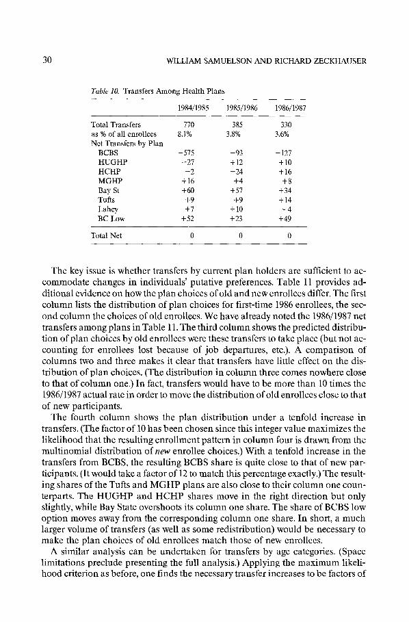
Direct data on individual transfers among plans provide further evidence on the incidence of status quo bias. Table 10 lists the total transfers and net transfers by plan between the years 1984/1985,1985/1986, and 1986/1987. In the last two periods, the percentages of transfers were 3.8% and 3.6%, respectively. The first-time availability of the BCBS low option plan in 1985 accounts for the larger transfer percentage, 8.1%, in 1984/1985. Some 466 of these transfers (amounting to 5%) were from BCBS to BCBS low option. While the total number of transfers is relatively small, the net transfers between plans are fewer still. Excepting transfers between the BCBS plans, no plan gained or lost more than 60 enrollees-less than 0.7% of the total-in any year. (If Bay State is excluded, the number is 27.)
30 WILLIAM SAMUELSON AND RICHARD ZECKHAUSER
Table IO. Transfers Among Health Plans
1984/1985 1985/1986 198611987
Total Transfers as % of all enrollees Net Transfers by Plan
BCBS HUGHP HCHP MGHP Bay St Tufts Lahey BC Low
110 385 330 8.1% 3.8% 3.6%
-575 -93 -127 -27 +12 +10
-2 -24 +16 +16 +4 +8 +60 +57 +34
+9 $9 +14 +7 +10 -4
+52 +23 +49
Total Net 0 0 0
The key issue is whether transfers by current plan holders are sufficient to ac- commodate changes in individuals’ putative preferences. Table 11 provides ad- ditional evidence on how the plan choices of old and new enrollees differ. The first column lists the distribution of plan choices for first-time 1986 enrollees, the sec- ond column the choices of old enrollees. We have already noted the 1986/1987 net transfers among plans in Table 11. The third column shows the predicted distribu- tion of plan choices by old enrollees were these transfers to take place (but not ac- counting for enrollees lost because of job departures, etc.). A comparison of columns two and three makes it clear that transfers have little effect on the dis- tribution of plan choices. (The distribution in column three comes nowhere close to that of column one.) In fact, transfers would have to be more than 10 times the 1986/1987 actual rate in order to move the distribution of old enrollees close to that of new participants.
The fourth column shows the plan distribution under a tenfold increase in transfers. (The factor of 10 has been chosen since this integer value maximizes the likelihood that the resulting enrollment pattern in column four is drawn from the multinomial distribution of new enrollee choices.) With a tenfold increase in the transfers from BCBS, the resulting BCBS share is quite close to that of new par- ticipants. (It would take a factor of 12 to match this percentage exactly.) The result- ing shares of the Tufts and MGHP plans are also close to their column one coun- terparts. The HUGHP and HCHP shares move in the right direction but only slightly, while Bay State overshoots its column one share. The share of BCBS low option moves away from the corresponding column one share. In short, a much larger volume of transfers (as well as some redistribution) would be necessary to make the plan choices of old enrollees match those of new enrollees.
A similar analysis can be undertaken for transfers by age categories. (Space limitations preclude presenting the full analysis.) Applying the maximum likeli- hood criterion as before, one finds the necessary transfer increases to be factors of

STATUS QUO BIAS IN DECISION MAKING 31
Table Il. Effects of 1986/1987 Transfers on Percentage Enrollments
Plan 1986 Enrollees All Others Add Transfers Add Transfers X 10
BCBS 9.8 31.0 29.2 13.2 HUGHP 48.2 31.7 31.9 39.1 HCHP 19.3 13.2 13.4 15.4 MGHP 3.6 2.1 2.8 3.8 Bay St 3.8 6.6 7.1 11.3 Tufts 3.4 1.2 1.4 3.2 Lahey 1.9 1.5 1.5 1.0 BC Low 5.5 6.2 6.9 13.0
Total 100.0 100.0 100.0 100.0
2,11,13, and 6 for the respective age categories. Two reasons account for the small size of the factor for the 21-31 age group. First, the preference differences between new and old enrollees in this group are relatively small. Second, the rate of transfer for this group is relatively high. These effects tend to reduce the incidence of status quo bias.
To sum up, a comparison of plan choices between new and old enrollees pro- vides strong evidence of status quo bias. Old enrollees persist in electing the in- cumbent plan, BCBS, much more frequently than do new enrollees, and enroll in the new HMO plans (as well as HUGHP and HCHP plans) much less frequently. The very low rate of transfer among plans is further evidence of status quo inertia. However, little or no bias is evident in transfers between BCBS plans.
2.2 TWCREF retirement funds
In 1986, the Teachers Insurance and Annuity Association (TWA) counted some 850,000 participants in its retirement plans. Besides determining the amount of his or her annual contribution, a participant’s principal decision is to divide his or her premium between the TIAA fund (a portfolio of bonds, commercial loans, mortgages, and real estate) and CREF (a broadly diversified common stock fund). Each year, a participant can change his or her distribution (applying to future, but not past, premiums) between the funds at no cost. It is this periodic decision that provides a natural test of status quo persistence.
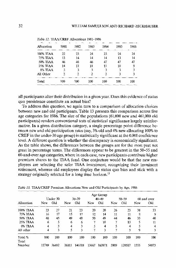
Table 12 shows the proportions of participants choosing particular premium allocations between TIAA and CREF for the years 1981-1986. Note that the changes in allocations year by year are insignificant-despite large variations in TIAA and CREF rates of return, in both absolute and relative terms. In fact, a TIM study (1986) finds that only 28% of those surveyed had ever changed their distribution of premium between the funds (8% had changed more than once, 20% exactly once). Given a 12-year average length of participation, fewer than 2.5% of
32 WILLIAM SAMUELSON AND RICHARD ZECKHAUSER
Tab/e 12. TIAA/CREF Allocations 1981-1986
Allocation 1981 1982 1983 1984 1985 1986
100% TIAA 22 23 24 23 24 24 75% TIAA 13 14 14 14 13 14 50% TIAA 46 46 46 47 47 47 25% TIAA 14 12 11 11 10 9
0% TIAA 3 3 3 3 3 3 All Other 2 2 2 2 3 3
Total 100 loo 100 100 100 100
all participants alter their distribution in a given year. Does this evidence of status quo persistence constitute an actual bias?
To address this question, we again turn to a comparison of allocation choices between new and old participants. Table 13 presents this comparison across five age categories for 1986. The size of the populations (61,000 new and 461,000 old participants) renders conventional tests of statistical significance largely uninfor- mative. In a given distribution category, a single percentage point difference be- tween new and old participation rates (say, 3% old and 4% new allocating 100% to CREF in the under-30 age group) is statistically significant at the 0.001 confidence level. A different question is whether the discrepancy is economically significant. As the table shows, the differences between the groups are for the most part not great in percentage terms. The differences appear to be greatest in the 50-55 and 60-and-over age categories, where in each case, new participants contribute higher premium shares to the TIAA fund. One conjecture would be that the new em- ployees are selecting the safer TIAA investment, recognizing their imminent retirement, whereas old employees display the status quo bias and stick with a strategy originally selected for a long time horizon.‘3
Table 13. TIAAKXEF Premium Allocations New and Old Participants by Age, 1986
Allocation
Age Group Under 30 30-39 40-49 50-59 60 and over
New Old New Old New Old New Old New Old
100% TIAA 23 27 21 23 20 20 26 23 38 33 15% TIAA 16 17 15 17 12 14 11 11 8 9 50% TIAA 48 45 49 48 50 49 44 46 35 40 25% TIAA 6 5 6 6 7 10 7 13 5 11
0% TIAA 4 3 4 3 5 4 5 4 5 4 All other 4 3 5 3 7 3 7 3 9 3
Total % Total Number
100 100 100 100 100 100 100 100 100 100
12749 36482 26111 146318 13667 163971 5909 120587 1553 54873

STATUS QUO BIAS IN DECISION MAKING 33
As noted earlier, one cannot test for status quo bias unless thte choices of new participants change significantly over time. Otherwise one would expect the un- changing behavior of old participants to track closely the unchanging behavior of new entrants. For most participants, the distribution of retirement contributions is a particularly thorny decision under uncertainty. According to TIAA’s 1986 survey results, almost all surveyed participants were aware that changes between the funds could be made annually at no cost. Nonetheless, participants found it dif- ficult to explain or justify their choices. For instance, only one in three participants surveyed felt his or her initial allocation was an informed choice. One in four said it was a guess, with the others characterizing it as something in between. (Indeed, almost half of all participants elect the simple allocation of 50% TIAA and 50% CREF.)
In light of this finding, it is difticult to characterize retention of the status quo allocation as a rational operating rule of thumb. Most of those who changed their allocation did so for a reason (primarily because of stock market performance). But very few participants had a particular reason for not changing their alloca- tion. As Samuel Johnson observed, it is easy to “decide” to do nothing.
Finally, the information provided by TIM may contribute to status quo persis- tence. Each participant receives an annual summary of plan performance and an illustrative calculation (with accompanying assumptions) of future accumulation at retirement age based on his or her current allocation. It would be a simple mat- ter for TIM to provide similar predictions under other premium allocations. One wonders what would happen if the comparison of alternative allocations failed to identify the participant’s current choice. Individuals’ bias for the status quo might be substantially reduced.
3. Explaining the status quo bias
Explanations for the status quo bias fall into three main categories. The effect may be seen as the consequence of (1) rational decision making in the presence of tran- sition costs and/or uncertainty; (2) cognitive misperceptions; and (3) psychologi- cal commitment stemming from misperceived sunk costs, regret avoidance, or a drive for consistency.
3.1 Rational decision making
Under several intepretations, an affinity for the status quo is perfectly consistent with rational decision making. For instance, consider decision makers who repli- cate their earlier choice in a second decision. A trivial explanation might be that they make the same decision because they are facing independent and identical decision settings (i.e., their preferences and choice sets are the same, or sufficiently similar, in each). In such a case, rationality requires them to make identical
34 WILLIAM SAMUELSON AND RICHARD ZECKHAUSER
choices. A more substantive explanation occurs when the sequential decisions are not independent-that is, the individual’s initial choice affects his or her preferen- ces or choice set in the subsequent decision. Transition costs, for example, may make any switch from the status quo costly in itself. Such transition costs in- troduce a status quo bias whenever the cost of switching exceeds the efficiency gain associated with a superior alternative.
Transition costs are pervasive and come in many forms. At the societal level, many nonproductive conventions endure mainly because any change would be costly. Thus, hundreds of languages persist worldwide despite the advantages in principle of a universal language such as Esperanto. More efficient alternatives seem to have little chance of replacing the classic typewriter keyboard.14 In the United States, nonmetric measurement persists despite metric’s clear advantage. More generally, many American institutions, such as the structure of public education and the four-year presidency, owe their existence largely to historical tradition and seem impervious to wholesale review or change.
Transition costs that support the status quo are prevalent in the private sector as well. Any economic transaction that requires an irreversible (or partially irrevers- ible) investment falls into this category. Because of the resource requirements in establishing, monitoring, and enforcing ongoing contracts, long-term buyer-seller agreements are to some degree resistant to competition. (If a member were to select a new partner, resources would have to be invested anew to establish a relation- ship.) Employer and worker are linked by mutual investments made in job- or firm-specific training. A buyer of a computer system is predisposed to favor the same or compatible systems in future purchases, since replacing it in toto may be prohibitively expensive.
A related explanation for status quo inertia is the presence of uncertainty in the decision-making setting. In the classic search problem, for example, the set of pos- sible choice alternatives is unknown before the fact: alternatives must be dis- covered. An individual may well stick to a low-paying job if the process of search- ing for a better one is slow, uncertain, and/or costly. Even when no explicit costs are associated with search or switching, uncertainty can lead to status quo inertia. Consider consumers who must choose one of many product brands. At the outset, they are uncertain about the utility they would derive from any brand. Only use will give them knowledge of a brand’s utility. Subsequently, they may switch brands and experience a different alternative. An optimal decision takes the form of a cutoff strategy: individuals stick with their current choice if their utility from it is sufficiently high; otherwise, they try another brand.
In some circumstances, following the optimal search rule can bestow a substan- tial advantage on a brand chosen early. For instance, Schmalensee (1982) analyzes a simple model in which a consumer must choose between two brands that are identical ex ante but offer uncertain utility. If the product proves to be reliable, consumers earn a high utility; if the product fails, they earn a low utility. While the initial choice of brand is a matter of indifference, consumers will remain loyal to the chosen brand in subsequent decisions if it proves reliable. Thus, if the chance
STATUS QUO BIAS IN DECISION MAKING 35
of failure is low, status quo inertia in consumer choices will be the norm.15 A model such as this helps explain why many families return to the same vacation spot each year (it is reliable, though not necessarily optimal). For similar reasons, many individuals buy the same model of automobile repeatedly and continue to pat- ronize the same mechanic.
One can describe a related reason for status quo persistence by replacing the cost of search with the cost of analysis in the earlier discussion. It has long been recognized that the choice to undertake a decision analysis is itself a decision. If the costs of such an analysis are high, it may well be optimal for individuals to per- form an analysis once, at their initial point of decision, and defer to the status quo choice in subsequent decisions, barring significant changes in the relevant cir- cumstances. Even individuals suffering from imperfect memory, who have forgot- ten the analysis behind their original decision, might rationally presume that the status quo choice was made on rational grounds. Consequently, they retain it, sav- ing the cost of reanalysis.
Since neither transition costs nor uncertainty plays an essential role in the hypothetical questions discussed in Section 1, the rational explanations are inade- quate to explain status quo inertia. Transition costs are ruled out either explicitly or by virtue of the decision context. (There is no cost to changing the budget alloca- tion, portfolio, bidding strategy, car color, or to building a new prison.16) Nor is there any obvious information asymmetry between the status quo choice and the new alternatives. Unless subjects were reading these factors into the decisions, the observed status quo effects cannot be explained as a rational decision response. One could hypothesize that the cost of analysis is a potential source of bias in several of the decision settings, particularly Questions 1 and 5. Since little or no in- formation is provided to choose between the safety budget allocations, a subject could plausibly retain the status quo, reasoning that it must have been picked for good reason. A similar inference might be drawn about expanding the old prison. In each case, the implicit rationality behind the status quo choice could be taken to outweigh the other pros and cons (such as they are described).
3.2 Cognitive misperceptions
In a variety of experimental settings, Kahneman and Tversky (1979, 1984) have shown that individuals weigh losses heavier than gains in making decisions. This phenomenon they label loss aversion. For example, in decisions whose outcomes are limited to monetary consequences, individual preferences are best described by a value function that is concave over monetary gains and convex over losses. (Thus, the individual is risk averse with respect to gains but risk seeking with re- spect to losses.) Since preferences depend on how outcomes are framed, this behavior violates the axioms of standard utility theory. Now consider the choice between retaining the status quo or opting for a new alternative. Taking the status quo as the reference point, the individual weighs potential losses from switching as
36 WILLIAM SAMUELSON AND RICHARD ZECKHALJSER
larger than potential gains. Because of loss aversion, the individual is biased in favor of the status quo. Thaler (1980), the first researcher to discuss this bias, calls it the endowment eflct.
Our findings of prevailing status quo bias parallel the experimental results test- ing loss aversion. However, there is an interesting and important difference. Status quo bias attributed to loss aversion depends directly on the framing of gains and losses. Thus, Thaler (1980) has argued that loss aversion explains the large positive differences found between individuals’ selling prices (the least compensation necessary to induce them to give up an item) and buying prices (the highest price willingly paid to obtain the item), and, more generally, reluctance to trade (Knetsch, Thaler, and Kahneman, 1987). Similarly, loss aversion contributes to status quo bias in multiattribute and intertemporal decisions (see Kahneman and Tversky, 1984; Quattrone and Tversky, 1987; Loewenstein, 1985). Consider a pair of alternatives involving two attributes, where each is better on one attribute and worse on the other. Most subjects assigned the first alternative as the status quo chose to retain it rather than switch. Those assigned the second alternative ex- hibited the same behavior. The framing of gains and losses in each case accounts for this result.
Our results show the presence of status quo bias even when there are no explicit gain/loss framing effects. Such framing is entirely absent in the budget problem, the car color choice, and the airline leasing decision. The job choice relies only on qualitative pros and cons. In the remaining Part One questions, quantitative infor- mation is provided but not framed in terms of gains and losses. (Nor does it appear that subjects could readily translate the descriptions mentally into gain/loss frames.) Thus, we conclude that status quo bias is a general experimental finding-consistent with, but not solely prompted by, loss aversion.
A second kind of fundamental cognitive misperception is termed anchoring. This effect is most obvious when the decision takes the form of choosing (or es- timating) an optimal value of one or more continuous variables, typically (but not limited to) some kind of quantity or price. A common strategy is to take an initial decision value as a starting point and to adjust this value in response to the economic facts of the problem to yield a hnal decision value. Though most such adjustments are in the right direction (i.e., toward the optimum) they are typically insufficient (see Tversky and Kahneman, 1974). Such anchoring might apply here to probabilistic forecasts that lead to a particular decision. As discussed earlier, the response rate results in Question 7 (water allocation) and version 3 of the fleet leas- ing question bear out this anchoring effect. Clearly, Questions 1,2, and 3 could be recast in continuous form to test for similar anchoring effects.
Finally, we note that a variant of anchoring can occur in decision tasks with dis- crete alternatives when, for reasons of bounded rationality, individuals undertake partial analysis of their available options. For instance, consider again the uni- versity employee in Section 2 who can choose among a number of alternative health plans. Since gaining a good understanding of the pros and cons of a single plan is a lengthy and complex undertaking, the individual can hardly be expected
STATUS QUO BIAS IN DECISION MAKING 37
to carry out a complete analysis of all plans. Assuming that he or she understands his or her current plan, a reasonable strategy would be to undertake a comparative analysis including only some subset of competing plans (ignoring the others altogether). Thus, the status quo alternative gains a decision advantage by virtue of the asymmetric position it holds in the decision reckoning.
3.3 Psychological commitment
A growing body of laboratory experiments conducted by psychologists and economists shows that, contrary to the model of rational man, individual choices are affected by sunk costs (and benefits). A good summary of this research is pro- vided by Brockner and Rubin (1982). In sequential decisions, continuance of status quo choices may be motivated by the individual’s reluctance to “cut his losses” or more generally by a desire to justify previous commitments to a (perhaps failing) course of action by making subsequent commitments. One of the earliest lessons in economics is that decisions should be based on incremental benefits and costs. Anyone who has taught this topic in an introductory course, however, knows that it must compete with an alternative intuition: the larger the past resource investment in a decision, the greater the inclination to continue the commitment in subsequent decisions. ” Thaler (1980) cites some familiar exam- ples: a subscriber who has prepaid for a concert series feels she must attend each concert despite conflicting engagements-but she would not attend if the tickets had been given to her free. To recover his annual membership fee, a yuppie con- tinues to play tennis three times a week, despite a painful tennis elbow. A car owner who has recently paid for new brakes and transmission reluctantly spends $1,000 for major engine repair.
Such anecdotal evidence can be supplemented with examples drawn from policy decisions. The investigation of the Teton Dam disaster found that the Bureau of Reclamation had never halted construction of a dam once started, de- spite safety flaws uncovered during construction. Lockheed continued to build the unprofitable L-101 1 aircraft (with the aid of Congressional funds) in a vain hope to recover its past investment. The day following the announcement of its can- cellation, Lockheed shares rose 18%. Many historians believe that the huge invest- ment in resources and lives helped motivate the continuing escalation of the Viet- nam conflict in the hope of gaining a military victory. Finally, it has been argued that the overriding consideration in Truman’s decision to use atomic weapons against Japan in World War II was that the billion dollars spent on the Manhattan project would be wasted if its “fruits” were not used to end the war (Schoenberger, 1979). Once it became clear that the Manhattan project would succeed, there was never any doubt in the minds of advisers and decision makers that atomic weapons would be used.‘*
As these examples illustrate, the presence of sunk costs or other resource in- vestments contributes to status quo bias in decision making. The greater the in- vestment in the status quo alternative, the more strongly it will be retained. Thus,
38 WILLIAM SAMUELSON AND RICHARD ZECKHAUSER
the degree of status quo bias in Question 4 (the job-switch decision facing the academic) may derive in part from the investment in time and effort made by the assistant professor at his current institution. One might predict that, all other things equal, the longer one has spent in a given job or profession, the less likely one is to switch. Similarly, in Question 5, a large capital investment in the current prison (no information on this point was provided) would induce a greater degree of status quo bias.
Another factor contributing to psychological commitment is regret avoidance. From time to time, individuals find themselves in the unpleasant position of regretting the outcomes of past decisions. Such lessons of experience teach them to avoid, if possible, regrettable consequences. In fact, there is substantial evidence (see Bell, 1982; Kahneman and Tversky, 1982) that regret avoidance influences decision making. Thus, individuals tend to avoid consequences in which they could appear after the fact to have made the wrong choice, even if in advance the decision appeared correct given the information available at the time. As Kahne- man and Tversky (1982) argue, individuals feel stronger regret for bad outcomes that are the consequence of new actions taken than for similar bad consequences resulting from inaction. I9 Avoidance of decision regret is thus one cause of status quo bias. It favors adherence to status quo norms or routine behavior at the ex- pense of innovation, and it reinforces to the individual’s inclination to conform to social norms. For instance, most parents would not dream of leaving a baby alone, sleeping in its crib, while they took a 15-minute auto trip to run an errand. In the extremely unlikely case that the child was killed in a fire, the parents would feel tremendous regret and guilt. However, many of the same parents would not hesi- tate to take the child along in the car, though the safety risk in the car is arguably an order of magnitude greater than in the house. The element of guilt associated with a bad consequence would be considerably less.*’ Norms may be more impor- tant in explicit social settings. Individuals often find that the path of least resis- tance is to conform to the institutional status quo-be it company policy, standard operating procedure, or the social norm-whether or not this constitutes an op- timal decision in the circumstances.
Many choices are made within group and organizational settings, where in- dividuals’ interests do not fully coincide. A decision maker may opt to retain a pre- vious choice to maintain his or her reputation and decision-making authority. To reverse his or her position might suggest that he or she had made a poor choice originally.
Of the decision tasks in Part One, decision regret would appear to be a factor in Questions 2,3, and 4. (In the other decision questions, the outcomes of actions not taken will remain unknown after the fact.) The individual would feel obvious regret for bad consequences that come with replacing his or her portfolio (possibly reinforced by family criticism), altering company bidding policy, or switching academic positions. In each of these questions, subject responses display a signifi- cant degree of status quo bias.
A drive for consistency can also create psychological commitment. The theory of

STATUS QUO BL4S IN DECISION MAKING 39
cognitive dissonance is central to many of the behavioral models employed by psy- chologists, sociologists, political scientists, and students of organizational be- havior.21 Indeed, it enjoys much the same status in social psychology that the model of rational, optimizing man holds in economics. With the notable excep- tion of Akerlof and Dickens (1982), few attempts have been made to incorporate this theory (and the accompanying empirical findings about individual behav- ior) into economic models. We believe that the individual’s drive to avoid cogni- tive dissonance in his or her role as decision maker contributes to status quo bias.
The basic tenet of cognitive dissonance theory is that the individual finds it dif- ficult to maintain two conflicting stances or ideas simultaneously and consequent- ly seeks cognitive consistency. One manifestation of this drive is a preference for certain beliefs-that is, individuals choose their beliefs in accordance with a wish to minimize cognitive dissonance. In particular, their interpretation of current in- formation and their receptivity to new sources of information are influenced in this way.
In the domain of personal choice, the individual is motivated to attain decision consistency. With his or her self-image as a serious and able decision maker comes a need to justify current and past decisions, whether or not they proved successful. Past choices are rationalized, and the rationalization process extends to current and future choices. Thus, an individual tends to discard or mentally suppress in- formation that indicates a past decision was in error (since such information would conflict with his or her self-image as a good decision maker).
Self-perception theory provides a closely related explanation for status quo persis- tence.22 The theory holds that individuals survey their own behavior much as an outsider would in order to draw inferences about their owyl underlying attitudes and preferences. (The economist will identify this notion as an instance of revealed preference applied to one’s own, presumably uncertain, preferences.) One manifestation of this kind of self-perception is to defer to past decisions as a guide to present and future choices. “If it was good enough for me then, it is (must be) good enough for me now.” By this reckoning, the individual tends to persist with the status quo. We noted earlier that adopting such a rule of thumb could well be a rational decision response in the presence of significant costs of analysis. In many cases, discrimination in decision making is costly; by its very nature, a rule of thumb is meant to be used indiscriminately and is therefore inexpensive. (There is a link here to situations where guidelines cannot be adjusted to each change in cir- cumstance. The fallback guideline is rule utilitarianism: selecting the rule that yields the highest value on average.) Certainly, the status quo is often maintained in the name of company policy, in adherence to standard operating routines, or for reasons of historical precedent or tradition.
It is difficult to disprove the hypothesis that adherence to the status quo may constitute rational behavior. Nonetheless, the psychological evidence on self- perception suggests the opposite conclusion. Experiments have shown that even where initial choices are imposed, subjects will create inferences suggesting that the

40 WILLIAM SAMUELSON AND RICHARD ZECKHAUSER
original choice was appropriate, (In similar fashion, randomly generated actions are self-perceived as satisfactory.) In drawing inferences from past behavior, in- dividuals fail to discriminate to some degree between imposed actions, random selections, and choices voluntarily (and thoughtfully) undertaken.
A classic experiment by Festinger and Carlsmith (1959) shows the effects of im- posed actions. Subjects were first required to perform long and tedious tasks in in- dividual sessions. Each subject was then paid to tell a waiting fellow student (a stooge) that the tasks were enjoyable and interesting. In one group, subjects were paid $1; in the other, they were paid $20. After the experiment, each subject in- dicated how much he or she had enjoyed the tasks. The results show that subjects paid $1 evaluated the tasks as significantly more enjoyable than subjects who were paid $20. Self-perception theory offers a cogent explanation of this anomalous result. Subjects draw inferences about their true attitudes by observing their ac- tions as an outsider would. Such an observer hears the statement that the task was pleasurable. A $1 payment does not seem sufficient financial incentive to induce the statement. Thus, the inference is that the statement is genuine. At $20 pay, the incentive to misrepresent appears sufficient so that no such inference can be made about the individual’s true attitude. Thus, the revealed preference for the task of $1 subjects is greater than that of $20 subjects. The strong message of this and a host of other experiments is that subjects often draw incorrect or misleading inferences from past actions.
Status quo bias in individual decision making is explained in part by cognitive dissonance theory. The act of choosing an alternative raises its value to some de- gree. Other things equal, this induces a bias toward retaining the choice in subse- quent decisions even under changed conditions. Moreover, the theory predicts that other things will not be equal. The individual will be biased in interpreting subsequent information in favor of the status quo choice. His or her propensity to retain the status quo option is increased. In a similar vein, self-perception theory promotes status quo inertia. Individuals who infer their attitudes and preferences from past actions (whether rationally chosen or not) will tend to persist in these actions. One could hypothesize that cognitive dissonance and self-perception theory are both potential explanations of status quo bias in the airline leasing problem. The latter theory could also explain status quo bias in the car color deci- sion, where the status quo choice is arbitrarily imposed.
A third type of psychological commitment contributing to status quo bias stems from efforts to feel in control. Making a decision enforces the individual’s percep- tion that he or she controls the situation. Langer (1983, pp. 68-72) describes a series of experiments in which subjects maintain the illusion of control by stick- ing with their status quo choices. Each of 27 subjects holds a football card. One of the 27 cards will be drawn randomly by lottery to determine which subject will win a $50 prize. In one (27-member) group, each subject is permitted to choose his or her card from a large pool of football cards. In another group, each subject is assigned a card. Before the lottery, each subject is asked to name a price for giving up his or her card. (The actuarially fair price is $1.85.) In the experiment, the aver-

STATUS QUO BIAS IN DECISION MAKING 41
age price in the “no choice” group was found to be $1.96 (about what one might ex- pect). But the average price in the “choice” group was $8.67, more than four times the fair price. The bias stemming from the illusion of control is a significant poten- tial source of status quo inertia.
In sum, status quo bias is pervasive. It is a natural consequence of many well- known psychologically based deviations from the rational choice model. As a result the canonical choice model is unlikely to provide a reliable explanation for a substantial range of behavior, including economic behavior.
4. Applications
The controlled experiments demonstrate that for a variety of decision situations individuals exhibit a significant and predictable status quo bias. This bias in- creases (in relative terms) with the number of choice alternatives. Although this af- finity for the status quo might be interpreted as a rational response to real transi- tion costs and to uncertain outcomes, the experiments (by abstracting from these factors) suggest strongly that the answer lies elsewhere. In our view, the best ex- planation is that the status quo choice acts as a psychological anchor. Roughly speaking, the stronger the individual’s previous commitment to the status quo, the stronger the anchoring effect.
As outlined in the previous section, a host of observable factors help explain status quo inertia. With these factors in mind, a natural next step in the analysis would be to characterize the potential strength of status quo effects across different decision settings. In this respect, the present approach has some advantages over other models of bounded or quasi-rationality. For instance, Simon’s (1957) model of satisticing behavior, while offering a plausible alternative to instantaneous op- timization, is far less satisfactory in generating testable predictions about be- havior. When and how do individuals satisfice? When they do, how great is the shortfall from optimal behavior? There is a strong parallel between the present analysis and the satisficing model; both account for suboptimal behavior. Our analysis, however, can trace the preconditions for and the extent of such behavior. Similarly, the status quo bias can be viewed as an obstacle in the transition to bet- ter allocational decisions. As such, it has the same effect as the transaction (or transition) cost so often invoked by economists. Here, however, costs to switch from the status quo are perceived by decision makers but not actually borne by them. Thus, the cost associated with status quo inertia is the welfare loss stemming from efficient decisions not taken. Should the individual succeed in making un- biased decisions, this cost would disappear.
We believe that a decision-making model incorporating status quo effects pro- vides a better description of economic behavior in many settings than does the stan- dard choice model with or without transaction costs. We conclude by noting several important economic applications of this model and by discussing its implications for individual decisions, public policymaking, and the advance of knowledge.

42 WILLIAM SAMUELSON AND RICHARD ZECKHAUSER
4.1 Periodic decisions
The field studies in Section 2 indicate the role of status quo bias in periodic or recurring decisions. Similarly, over extended periods of time, individuals tend to retain unchanging dollar amounts of insurance (auto, house, or life) from the same provider, make standard contributions to savings accounts, and so on. Fund- raisers for schools and charities exploit status quo effects in their efforts to max- imize revenues. The most important determinant of an individual’s lifetime con- tribution is the early establishment of an unbroken chain of year-by-year gifts. Once initiated, a year-by-year donation becomes firmly entrenched as the status quo. Thus, fund-raisers emphasize donation frequency rather than size in their campaigns.
For example, Pacific Gas and Electric Company sought to determine residen- tial customers’ preferences relating to interruptable-rate electricity schedules. It surveyed 2,200 households, asking each to choose among six schedules. A prob- abilistic choice model, using contract and customer attributes as explanatory variables, found that current choice was the most important predictor of the service schedule chosen. Customers were reluctant to give up their existing service schedule to get cheaper rates. (This explains the high outage costs implied by the choice of service option, costs that far exceed customer survey results.) The authors conclude that recognizing the status quo effect is crucial for decisions on utility capacity and rates (Doane et al., 1987).
4.2 Search
Status quo effects also have direct implications for the theory and practice of search. Status quo bias could be expected to lead individuals and firms to partake in less search than would be optimal. (Schotter and Braunstein (1981) found evidence of theoretically insufficient search in several experiments.) Search pro- cesses are central to models of technological innovation. For instance, the evolutionary theory of economic change advanced by Nelson and Winter (1982) posits nonoptimizing firms that undertake adaptive search over alternative technologies and production plans. This search combined with the economic natural selection of more profitable firms generates convergence to a prolit- maximizing economic equilibrium. If status quo effects impede firms’ adaptive search, such an equilibrium may not be attained, particularly if there is some con- tinuing change in the environment.
In consumption decisions under uncertainty, searches by individuals for better prices induce competition among firms. Thus, given optimal search on the part of consumers, one can predict that price dispersion among competing firms will vary substantially with search costs. However, a study by Pratt, Wise, and Zeckhauser (1979) found that across a large sample of different products, the standard devia- tion of competing prices varies directly with price. Large-ticket items show a much
STATUS QUO BIAS IN DECISION MAKING 43
greater price dispersion than small-ticket items. Search costs do not vary suflicien- tly with the prices of products to explain this finding. The standard search model tells at most only a small part of the story. The pattern is consistent, however, with the presence of status quo bias. If the offer received at the first or second store becomes the status quo, for example, the customer may choose not to search further. To the extent that rational consumer search is impeded, greater price dis- persion will be the equilibrium result. (Insufficient effort to search for high-price goods may also be explained by consumer tendencies to measure and value price gains in percentage rather than absolute terms.)
4.3 Soft selling
A variety of soft-sell techniques used in business exploit status quo effects. Many of the most effective techniques lead the consumer to make a psychological invest- ment in the buying process. For instance, Thaler (1980) points out that a common inducement is the trial purchase without obligation; the item may be returned for a full refund. To the consumer, this appears to be a “no lose” proposition. Arguably it is, but for the seller. For the duration of the purchase, consumers abandon the search for better alternatives, while increasing their psychological investment in the purchase. In their self-perception, they made the purchase for a deliberate pur- pose: not simply as a trial, but because the item satisfied their needs. The epitome of this device is the free baby picture offer. (The proud parents are under no obligation to buy the other portraits. But look how cute they are. Isn’t it a shame that the shots will be wasted?) Similarly, order-takers always try to obtain a deposit from the customer, not because it is necessary to reserve an item, but because it is the surest way to secure a sale. The deposit can be completely refund- able or can be for a nominal amount; the key is to induce the consumer to part with it.
A variant of these practices occurs in the pricing of multiple telephone and cable television service options. Providers of these services typically charge cus- tomers a one-time transition fee for switches to an upgraded package (e.g., adding cable channels) but levy no transition fee for downgrading. In this way they hope to persuade the customer that it is wise to begin with the upgraded package for a trial period. Thus, these expensive packages become (and subsequently remain) the status quo alternative for a predictable number of customers.
A final tying tactic is typified by the S&H green stamp and frequent flyer pro- grams. It would appear that travelers are tied to their chosen airlines as much by il- lusory factors as by real ones. By offering large mileage bonuses upon initial en- rollment and by setting many intermediate awards as mileage accumulates, airlines’ coupon plans emphasize pseudosunk costs and offer plan members strong psychological inducements to accumulate mileage, even though the ul- timate awards are small.
44 WILLIAM SAhKJELSON AND RICHARD ZECKHAUSER
4.4 Sticky prices and exit barriers
The presence of status quo bias, like real transition costs, introduces friction into otherwise fiictionless economic models of resource allocation. Thus, this model would predict significant inertia in the movement of resources in response to market signals. At the most fundamental level, status quo framing has a signiti- cant influence on the determination of wages paid to labor. Negotiating percent- age wage increases over three-year labor contracts is quite a different thing from negotiating wage levels year by year. (The recent record of wage negotiations sug- gests that management has succeeded in part in turning the focus toward levels.) Recent research by Kahneman, Knetsch, and Thaler (1986) indicates that con- sumers and producers view the terms of current (i.e., status quo) transactions as entitlements that govern community standards of fairness when it comes to changes in these terms. This notion of status quo entitlements explains why the ad- justment of prices and wages is sluggish and incomplete (and not a continuous auction). The authors find that, according to community standards, it is accept- able for firms to raise prices if profits are threatened or to maintain prices when costs diminish. But it is unfair to exploit shifts in demand by raising prices or cut- ting wages. Thus, interpretations of fair price adjustments vis-a-vis the status quo provide a partial answer to one of the enduring questions in economics: why wages exhibit downward stickiness in the presence of unemployment.
Our results also imply that the exit of firms from industries or product lines or of workers from jobs will be slower and less frequent than would be predicted by the canonical choice model, with and without transition costs. The management science literature contains ample evidence of management’s reluctance to ter- minate unprofitable products, sell loss-making divisions, or leave noncompetitive industries. While workers show considerable mobility between jobs and across geographic regions, studies indicate there is considerably less lifetime mobility be- tween professions-less, in our view than can be accounted for by the canonical model, even including job-change costs and nontransferable investments in job training and human capital. A dramatic example is provided by workers in high- risk occupations. Many long-time benzene workers, when interviewed, rational- ized their job choice by denying any abnormal risk (Ben-Horin, 1979). This rationalization persisted despite freely available information about job-related safety risks.
4.5 Market competition
Consumers display brand loyalty for a host of products. Indeed, a major objective of firms’ marketing and advertising is to create and maintain brand loyalty. In re- cent years, stochastic models of brand-switching have sought to describe the statis- tical properties of this behavior. Recent findings in this area (for example, Jeuland, 1979) suggest there is considerable brand choice inertia. That is, initial purchase
STATUS QUO BIAS IN DECISION MAKING 45
and use of a brand significantly increase the likelihood of repurchase in a subse- quent consumption decision. Clearly, status quo effects contribute to this behavior.
Status quo bias may also help explain the empirical finding that pioneering brands earn a long-run market share advantage (Urban et al., 1986). Although a number of contributing factors-product positioning and marketing advantages, brand name recognition, learning curve effects-have been suggested as ex- planations, no empirical studies have yet pinpointed the sources of the pioneer’s advantage. Clearly, status quo bias is a potential factor in such an explanation. Urban et al. (1986) present empirical estimates showing that the pioneering brand obtains a market share of 58.5% after a second firm enters, 43.6% after a third firm enters, and 35.7% after a fourth firm enters. Is it merely a coincidence that these es- timates are close to the experimental predictions in Section l?
Finally, recognition of status quo bias suggests a novel conjecture about the measurement of market competition-one that runs contrary to the standard economic prediction. If status quo effects are significant, it could well be that an increase in the number of competitors reduces the degree of market competition. That is, with the entrance of new firms, dominant producers (those with dispropor- tionate market shares) may become more dominant. For instance, the enormous number of producers and products in the rapidly growing personal computer market undoubtedly contributed to the emergence of IBM as the industry stan- dard. A similar phenomenon may account for the state of competition in the long- distance telephone market. Households across the country have been asked to select via ballot their preferred long-distance carrier. In some parts of the country, consumers can choose from more than 15 companies. This competition not- withstanding, returns to date show that AT&T (the status quo alternative for most consumers) will be chosen by 75% to 80% of all customers. This outcome is under- standable in view of the large numbers and relatively small individual sizes of AT&T’s competitors. (Presumably, AT&T would prefer to have numerous small competitors rather than a few more formidable rivals accounting for the same market share.) Thus, in the presence of status quo effects, more numerous alter- natives may not bring either better-informed consumer choices or increased competition.
4.6 Public policy
Status quo effects also influence policymaking within organizations, both public and private. Once made, policies frequently persist and become codified implicitly or explicitly in the form of decision-making rules of thumb, company policy, stan- dard operating procedures, and the like. Public program review is an important case in point. Far less than 1% of the funds allocated to public programs is devoted to program review or performance evaluations. When Gilbert, Light, and Mos- teller (1977) reviewed 29 large-scale social programs (including the Salk vaccina-
46 WILLIAM SAMUELSON AND RICHARD ZECKHAUSER
tion program and the New Jersey negative income tax experiment), they found the vast majority of program evaluations to be inconclusive respecting the relative benefits and costs of the programs. Nonetheless, policymakers were inclined to view these programs as successes, and program evaluations (such as they were) buttressed this belief. Of course, many programs receive little or no evaluation. Without such evaluation, given the difficulty of terminating spending on items that have become part of an authorized budget, long-standing programs often have a life of their own (though they would have little chance of passing a new pro- gram cost-benefit test).
Status quo effects are likely to be of significance in the domain of negotiated public policy outcomes. The presence of multiple interests creates a different pres- sure for sticking with the status quo. The Coase theorem holds that, in the absence of markets, assuming zero transaction costs, economic efficiency can be achieved by means of voluntary negotiated agreements. To the extent that status quo effects impede such agreements, this conclusion will be attenuated. For instance, the failure to reach negotiated agreements between state governments and towns for the location of hazardous waste processing facilities has been extensively docu- mented by O’Hare et al. (1983). To the extent that property rights become es- tablished in the status quo, any attempt to move away will be blocked. Economists are prone to talk about potential Pareto improvements, side payments, and the like. But the world prohibits cash side payments in many contexts, in-kind payments are too inefficient, and potentially compensable changes have no moral standing. The status quo persists, and those who propose a change merely incur the wrath of others.
Indeed, preference reversals are often observed in the valuation of public goods where entitlements are involved. Thus, it is not uncommon that an individual’s (or a community’s) required compensation for bearing a negative externality is an order of magnitude greater than its willingness to pay for relief from the same ex- ternality. Rowe, d’Arge, and Brookshire (1980) provide empirical estimates of these compensating measures for individual valuation of improved visibility due to reduced air pollution. Although other explanations (income and endowment ef- fects) are possible, these reversals are easily accounted for by significant status quo bias.
4.7 Scien t$c advancement
The progress of science is commonly perceived as a continuous, incremental ad- vance, as new discoveries are added to the accumulated body of scientific knowl- edge. However, Thomas Kuhn (1962) has argued that the history of science tells a different story, in which discontinuities are crucial. Science proceeds by a series of revolutions. A prevailing theory or paradigm is not overthrown by the accumula- tion of contrary evidence but rather by a new paradigm that, for whatever reasons, begins to be accepted by scientists. Between such revolutions, old ideas and beliefs persist and form barriers of resistance to alternative explanations.
STATUS QUO BIAS IN DECISION MAKING 47
As Kuhn notes, the men who called Copernicus mad because he proclaimed that the earth moved were not just wrong. More to the point, what they meant by earth was fixed position. Their earth could not move. A similar example occurs much later in the history of astronomy. The planet Uranus was discovered (that is, recognized as a planet) only after being variously sighted and then dismissed dur- ing the preceding 90 years by 17 observers, all influenced by the prevailing view that there were, and could be, no planets in that region of the solar system. In other scientific fields, Lavoisier’s oxygen law met strong resistance from phlogiston theory. Newtonian mechanics clashed with older, time-honored explanations of gravity. More recently, Einstein’s general theory was slow to be accepted by the scientific community. Many of its new proponents were attracted largely on aesthetic, not evidential, grounds. In these cases, the battle between old and new theories was resolved not by the power of proof, by verification or falsification, but ultimately by degree of belief. Perhaps this observation should give pause to con- temporary economists. Have we so enshrined rationality that we fail to acknowl- edge important psychological factors in behavior?
In this view, scientific scholars are subject to status quo persistence. Far from being objective decoders of the empirical evidence, scientists have decided pref- erences about the scientific beliefs they hold. From a psychological perspective, this preference for beliefs can be seen as a reaction to the tensions caused by cogni- tive dissonance. Moreover, it is a common observation that in the practice of “nor- mal” science (to use Kuhn’s term), scientists will have accumulated a significant investment in received theory. From the viewpoint of science as a whole, these in- vestments might rightly be viewed as sunk costs and so be written off in the face of superior theories and methods. But this is hardly the case for the individual scien- tist, who may find it impossible to abandon his or her old work and be “born again” into a new scientific paradigm. An apt expression of status quo persistence is captured in a well-known statement by Max Planck. In his autobiography, he writes that “a new scientific truth does not triumph by convincing its opponents and making them see the light, but rather because its opponents eventually die, and a new generation grows up that is familiar with it.” Or, as Aldous Huxley said, “It is the fate of new truths to begin as heresies and end as superstitions.”
5. Conclusions
In choosing among alternatives individuals display a bias toward sticking with the status quo. Survey results using questionnaires confirm findings derived from ob- serving economic phenomena and the tabulations of actual choices on retirement and health plans. Rational explanations can be provided for the status quo bias. However, a variety of psychologically based theories provide more robust ex- planations; that is, their more specific predictions are validated. The two classes of explanations, we believe, are complementary. Assuming the status quo bias proves important, rational models will present excessively radical conclusions, exaggerat- ing individuals’ responses to changing economic variables and predicting greater
48 WILLIAM SAMUELSON AND RICHARD ZECKHAUSER
instability than is observed in the world. Status quo effects account for diverse economic phenomena: the difficulty of changing public policies, preferred types of marketing techniques, and the nature of competition in markets.
Samuelson’s research was supported by NSF grant SES8511221. Zeckhauser’s research was supported by the Business and Government Research Center, Harvard University. We thank Beth Quigley, Har- vard University, and Stuart Whalen and James M. Mulanaphy, TIAA-CREF, for providing us with data. Paul Andreassen, Michael Barzelay, Robert Klitgaard, George Loewenstein, Yasuhiro Sakai, Thomas Schelling, Kenneth Shepsle, Richard Thaler, Amos Tversky, Ray Vernon, W. Kip Viscusi, and participants in seminars at the University of California, San Diego, UCLA, Boston University, Harvard University, University of Maryland, the Nikko Conference on International Economics, and the Inter- national Symposium on Forecasting (Boston) provided helpful comments.
Notes
1. Readers familiar with the experimental research on decision making under uncertainty will recognize framing as an important influence with respect to individual probabilistic prediction (Tversky and Kahneman, 1974) and preference assessment (Kahneman and Tversky, 1979). Our study owes a considerable intellectual debt to the growing body of research in experimental psychology and economics aimed at testing the normative model of rational decision making. For collected articles in this area, see Kahneman, Slavic, and Tversky (1982).
2. But see also Quattrone and Tversky (1987) for other evidence on incumbency effects. 3. Robert Klitgaard remarked to us that it was particularly surprising to find a status quo bias in such
a wide range of settings given the frequently expressed penchant to search for variety in some cir- cumstances, leading to such expressions as: “Variety is the spice is life,” and “The grass is always greener.”
4. This anecdote is borrowed from O’Hare et al. (1983). 5. See Louis (1981). 6. For an account of Coke’s marketing travails, see “Saying No to New Coke” (1985). 7. We chose to list the status quo option first (rather than to randomly place it among the other op-
tions) in order to minimize subject confusion about which alternative was the status quo. Clearly, an order effect could potentially contribute to the finding of status quo bias. However, order effects were found to be nonexistent both for choices in the neutral setting and among the alternatives to the SQ op- tion (where in each case the order of alternatives was permuted).
8. We chose a linear regression model as a simple description of the pattern of status quo bias. Our tests of hypotheses should be interpreted cautiously. For instance, the dependent and independent variables, shown as percentages, are necessarily constrained to fall between 0 and 1; the regression analysis does not recognize these constraints. (As a practical matter, this did not prove to be a problem in our regression predictions.) An alternative would be to perform a logit analysis on the responses. Because of data limitations, we pooled the responses to all Part One questions and did not include dummies for individual questions.
9. Linear specifications satisfy these essential adding-up constraints, while others (for example, a log-linear specification) do not. This provides a further justification for the linear form.
10. This pattern of responses could also be explained as a kind of forecast adjustment. For instance, it is possible that subjects might put less trust in a period-two forecast of good conditions when con- ditions had been bad in the first period than they would in a favorable forecast for the first period. Con- sequently, the subjects would rationally choose smaller fleets in the former case than in the latter. The wording of our problem was designed to minimize this effect by stating (in the second year) that the first year’s forecast had been on target. This information should allow subjects to be more confident of second-year forecasts, counteracting the aforementioned effect.
STATUS QUO BIAS IN DECISION MAKING 49
11. The distributions of plan choices for 1986 and 198.5 enrollees were not significantly different from one another. Therefore, in the interest of increasing the sample size, the two populations were combined.
12. For the age group 21-31, there were very few enrollees before 1980. The reason is simple. Such in- dividuals would have been no older than 2.5 when hired. This group is small to begin with. The number electing a health plan and employed by the university six or more years later is smaller still. Again, for reasons of sample size, we have grouped all enrollees in 1982 or earlier as the “old” group.
13. The differences in allocations would be more dramatic if “all other” allocations were removed from the analysis.
14. See David (1985) for an illuminating account of the history of the standard keyboard. See Schell- ing (1960) for a more general discussion of how individuals tacitly coordinate their choices.
15. It is important to note, however, that in two-armed bandit problems (Degroot, 1970) an optimal strategy for the individual calls for sampling alternative choices from time to time, even when extensive experience with the status quo alternative indicates that in all probability it is superior. To take a simple example, the reluctance of individuals to sample (or resample) new foods not included in their regular diet flies in the face of optimal sampling behavior. Certainly, the lunchtime diner in our earlier exam- ple, admittedly an extreme case, should have sampled new fare at least occasionally over the decades. In real-life situations resembling bandit problems, we would conjecture, very few people approximate an optimal strategy. Quite apart from status quo bias, we believe the strategy to be strongly counterintuitive.
16. In response to queries from seminar participants about the potential significance of transition costs, we presented alternatively worded versions of Questions 2, 3, and 6 and the aircraft question to subsets of subjects. In each case, the alternative version was written to minimize the suggestion of tran- sition costs. These alternatives are listed (in brackets) in the Appendix. In all cases, subject responses were insignificantly different across the versions. The figures shown in Tables 1 and 8 combine the results of all versions.
17. A simple classroom experiment, conducted on a number of occasions at Boston University, pre- sents a good illustration of the same bias on the production side of the model. Half the class receives a handout describing the pros and cons of launching a new product (which requires a significant mone- tary investment). Subjects record their decisions to launch or not. Since the pros greatly outnumber (and outweigh) the cons, over 90% of students launch the product. These students then receive a second handout describing events one year later. They learn that results to date have been unpromising; the cons now seem to outweigh the pros. Should the company continue its investment (a magnitude com- parable to the previous year’s) in the product? About 60% of students answer yes. The other half of the class receives an initial handout containing exactly the same one-year-later information, except that the first investment decision has been made for them by another management group within the company. Only about 35% of these students decide to continue the investment. One concludes that the initial in- vestment decision (an eminently rational one given the circumstances) causes a strong psychological commitment to continue the investment.
18. See Stimson (1947) however, for the argument that the decision to use atomic weapons was based solely on estimates of benefits and costs.
19. As an example, suppose you own stock worth $1,000 in Company A and can exchange it for $1,000 of stock in Company B. Given your investment assessment, you choose to hold your current shares. Your neighbor holds $1,000 in Company B and, for reasons similar to yours, decides to switch his shares for $1,000 of Company A. During the next six months, the value of each person’s stock in Company A falls to $700. Which one feels the greater regret?
20. Social norms may evolve to conform to market opportunities. In Europe, where the babysitter market is less developed, we are told, it is more acceptable for parents to leave children unattended for short periods. Victor Fuchs is undertaking interesting work on the demand for social norms in his assessment of gender relationships.
21. Our discussion can only provide a brief outline of cognitive dissonance theory. Indeed, what we speak of as a theory is better understood as a number of fundamental hypotheses about human
50 WILLIAM SAMUELSON AND RICHARD ZECKHAUSER
behavior that have been tested and confirmed by an extensive body of psychological experiments. Ap- plications and discussions can be found in Brehm (1956). Knox and Inkster (1968) and Bern (1972).
22. Bern (1972) provides a readable survey and overview of self-perception theory.
References
Akerlof, G. A. and Dickens, W. T. “The Economic Consequences of Cognitive Dissonance,“American Economic Review 72 (1982) 307-319.
Bell, D. E. “Regret in Decision Making Under Uncertainty,” Operations Research 30 (1982), 961-981. Bern, D. J. “Self-Perception Theory.” In: L. Berkowitz, ed., Advances in Experimental Social Psychology,
Vol. 6, Academic Press, 1972. Ben-Horin, D. “Dying to Work: Occupational Cynicism Plagues Chemical Workers,“Zn These Times 3
(June 27/July 3, 1979) 24. Brehm, J. “Postdecision Changes in the Desirability of Alternatives,” Journal of Abnormal Social Psy-
chology 52 (1956), 384-389. Brockner, J., and Rubin J. Z. Entrapment in Escalating Conflict. Springer-Verlag, 1982. David, P. “Clio and the Economics of QWERTY,” American Economic Review 75 (1985), 332-337. Degroot, M. Optimal Statistical Decisions. New York: McGraw-Hill, 1970. Doane, M. J., Hartman, R. S., and Woo, C. “Household Preference for Interruptible Rate Options and
the Revealed Value of Service Reliability,” mimeo, Boston University, 1987. Festinger, L., and Carlsmith, J. M. “Cognitive Consequences of Forced Compliance,” Journal ofAbnor-
ma1 and Social Psychology 58 (1959) 203-210. Gilbert, J. P., Light, R. J., and Mosteller, F. “Assessing Social Innovations: An Empirical Base for
Policy.” In: W. Fairley and F. Mosteller, eds., Statistics and Public Policy. Reading, Massachusetts: Addison-Wesley, 1977.
Jeuland, A P. “Brand Choice Inertia as One Aspect of the Notion of Brand Loyalty,” Management Science 25 (1979), 671-82.
Kahneman, D., Knetsch, J. L., and Thaler, R. “Fairness as a Constraint on Profit Seeking: Entitlements in the Market,” American Economic Review 76 (1986) 728-741.
Kahneman, D., Slavic, P., and Tversky, A. Judgment Under Uncertainq: Heuristics and Biases. Cam- bridge, England: Cambridge University Press, 1982.
Kahneman, D., and Tversky, A “Prospect Theory: An Analysis of Decision under Risk,” Econometrica 47 (1979) 263-281.
Kahneman, D., and Tversky, A. “The Psychology of Preference,” ScientiJicAmerican 246 (1982), 160-173. Kahneman, D., and Tversky, A “Choices, Values and Frames,“American Psychologist 39 (1984), 341-350. Knetsch, J., Thaler, R., and Kahneman, D. “Reluctance to Trade: An Experimental Refutation of the
Coase Theorem,” mimeo, 1987. Knox, R. E., and Inkster, J. A., “Post Decision Dissonance at Post Time,” Journal of Personality and So-
cial Psychology 8 (1968) 319-323. Kuhn, T. P. The Structure of Scientific Revolutions. Chicago: Chicago University Press, 1962. Langer, E. The Psychology of Control. Beverley Hills, CA: Sage Publications, 1983. Loewenstein, G. “Expectations and Intertemporal Choice,” Economics dissertation, Yale Universi-
ty, 1985. Louis, A M. ‘Schlitz’s Crafty Taste Test,” Fortune (June 26, 1981) 32-34. Mulanaphy, J. “Participants’ Allocation Change and CREF Transfer Practices,” Teachers Insurance
and Annuity Association, 1986. Neipp, J., and Zeckhauser, R. “Persistence in the Choice of Health Plans.” In R. Scheffler and L.
Rossiter, eds., Biased Selection in Health Care Markets. Greenwich, CT: JAI Press, 1985. Nelson, R., and Winter, S.An Evolutionary Theory ofEconomic Change. Cambridge, Massachusetts: Har-
vard University Press, 1982.
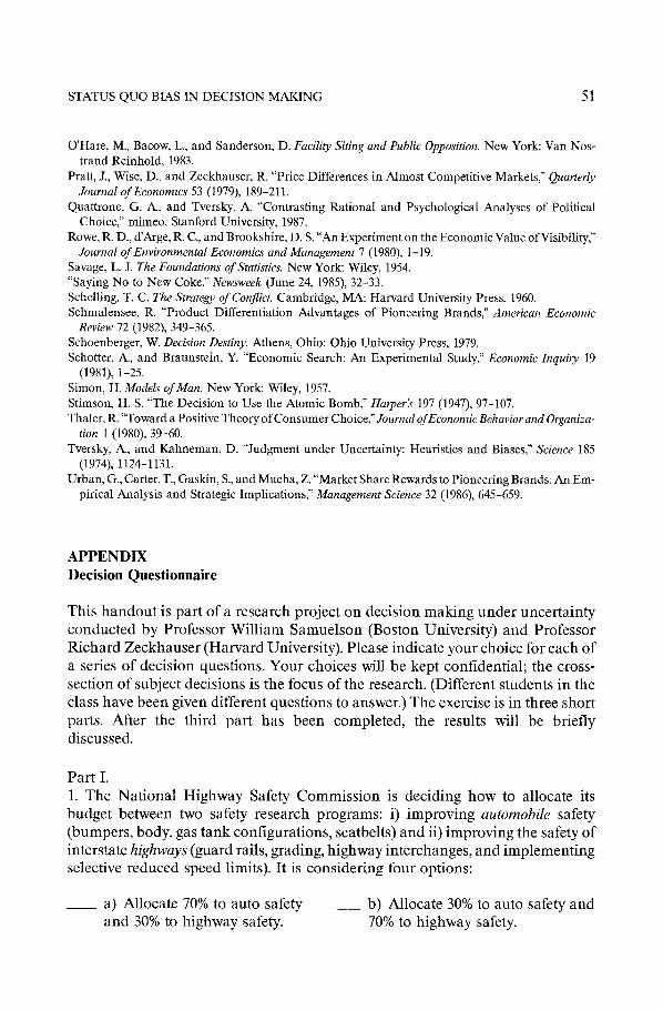
STATUS QUO BIAS IN DECISION MAKING 51
O’Hare, M., Bacow. L., and Sanderson, D. Facility Siting and Public Opposition. New York: Van Nos- trand Reinhold, 1983.
Pratt, J., Wise, D.. and Zeckhauser, R. “Price Differences in Almost Competitive Markets,” Quarterly Journal of Economics 53 (1979), 189-211.
Qua&one, G. A., and Tversky, A. “Contrasting Rational and Psychological Analyses of Political Choice,” mimeo, Stanford University, 1987.
Rowe, R. D., d’Arge, R. C., and Brookshire, D. S. “An Experiment on the Economic Value of Visibility,” Journal of Environmental Economics and Management 7 (1980) 1-19.
Savage, L. J. The Fourldations of Statistics. New York: Wiley, 1954. “Saying No to New Coke,” Newsweek (June 24, 1985), 32-33. Schelling, T. C. The Strategy of Conflict. Cambridge, MA: Harvard University Press. 1960. Schmalensee, R. “Product Differentiation Advantages of Pioneering Brands,” American Economic
Review 72 (1982), 349-365. Schoenberger, W. Decision Destiny. Athens, Ohio: Ohio University Press, 1979. Schotter, A., and Braunstein, Y. “Economic Search: An Experimental Study,” Economic Inquiry 19
(1981), l-25. Simon, H. Models of Man. New York: Wiley, 1957. Stimson, H. S. “The Decision to Use the Atomic Bomb,” Hurperk 197 (1947), 97-107. Thaler, R. “Toward a Positive Theory of Consumer Choice,” Journal ofEconomic Behavior and Organiza-
tion 1 (1980), 39-60. Tversky, A., and Kahneman, D. “Judgment under Uncertainty: Heuristics and Biases,” Science 185
(1974), 1124-1131. Urban, G., Carter, T., Gaskin, S.. and Mucha, Z. “Market Share Rewards to Pioneering Brands: An Em-
pirical Analysis and Strategic Implications,” Managemeflt Scietlce 32 (1986), 645-659.
APPENDIX Decision Questionnaire
This handout is part of a research project on decision making under uncertainty conducted by Professor William Samuelson (Boston University) and Professor Richard Zeckhauser (Harvard University). Please indicate your choice for each of a series of decision questions. Your choices will be kept confidential; the cross- section of subject decisions is the focus of the research. (Different students in the class have been given different questions to answer.) The exercise is in three short parts. After the third part has been completed, the results will be briefly discussed.
Part I. 1. The National Highway Safety Commission is deciding how to allocate its budget between two safety research programs: i) improving automobile safety (bumpers, body, gas tank configurations, seatbelts) and ii) improving the safety of interstate highways (guard rails, grading, highway interchanges, and implementing selective reduced speed limits). It is considering four options:
- a) Allocate 70% to auto safety - b) Allocate 30% to auto safety and and 30% to highway safety. 70% to highway safety.
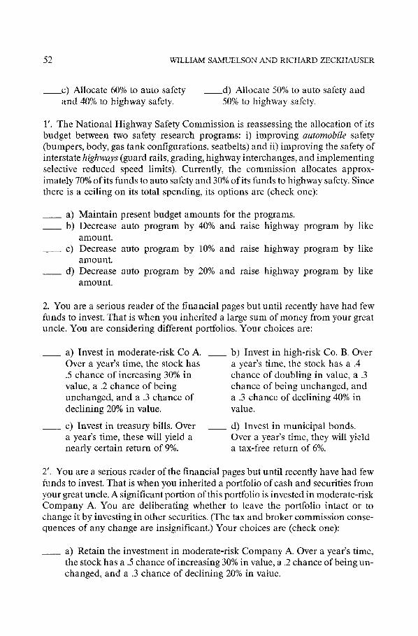
52 WILLIAM SAhJUELSBN MD RICHARD ZECKHALJSER
-c) Allocate 60% to auto safety -d) Allocate 50% to auto safety and and 40% to highway safety. 50% to highway safety.
1’. The National Highway Safety Commission is reassessing the allocation of its budget between two safety research programs: i) improving automobile safety (bumpers, body, gas tank configurations, seatbelts) and ii) improving the safety of interstate highways (guard rails, grading, highway interchanges, and implementing selective reduced speed limits). Currently, the commission allocates approx- imately 70% of its funds to auto safety and 30% of its funds to highway safety. Since there is a ceiling on its total spending, its options are (check one):
- a) Maintain present budget amounts for the programs. ___ b) Decrease auto program by 40% and raise highway program by like
amount. - c) Decrease auto program by 10% and raise highway program by like
amount. - d) Decrease auto program by 20% and raise highway program by like
amount.
2. You are a serious reader of the financial pages but until recently have had few funds to invest. That is when you inherited a large sum of money from your great uncle. You are considering different portfolios. Your choices are:
- a) Invest in moderate-risk Co A. - b) Invest in high-risk Co. B. Over Over a year’s time, the stock has a year’s time, the stock has a .4 .5 chance of increasing 30% in chance of doubling in value, a .3 value, a .2 chance of being chance of being unchanged, and unchanged, and a .3 chance of a .3 chance of declining 40% in declining 20% in value. value.
- c) Invest in treasury bills. Over - d) Invest in municipal bonds. a year’s time, these will yield a Over a year’s time, they will yield nearly certain return of 9%. a tax-free return of 6%.
2’. You are a serious reader of the financial pages but until recently have had few funds to invest. That is when you inherited a portfolio of cash and securities from your great uncle. A significant portion of this portfolio is invested in moderate-risk Company A. You are deliberating whether to leave the portfolio intact or to change it by investing in other securities. (The tax and broker commission conse- quences of any change are insignificant.) Your choices are (check one):
- a) Retain the investment in moderate-risk Company A. Over a year’s time, the stock has a .5 chance of increasing 30% in value, a .2 chance of being un- changed, and a .3 chance of declining 20% in value.
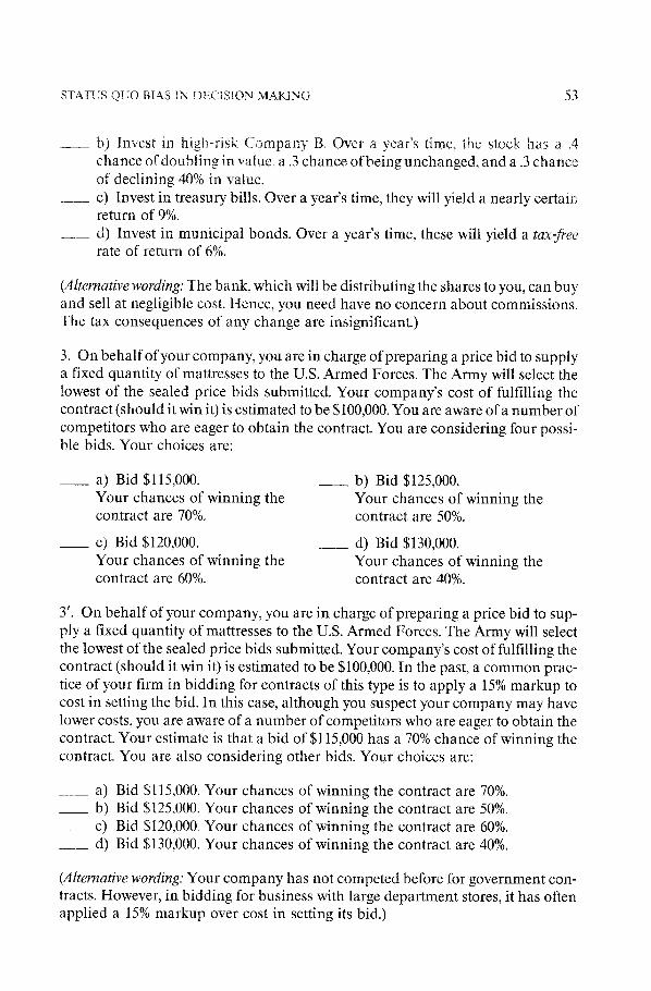
.- b) Invest in highrisk: !brqm-q- R. Over a year‘s time. the stock has a .4 chance of doubling in value. a .3 chance of being unchanged, and a .3 chance of declining 40% in value.
__ c) Invest in treasury bills. Over a year’s time, they will yield a nearly certain return of 9%.
__ d) Invest in municipal bonds. Over a year’s time, these will yield a tax-jkee rate of return of 6%.
(Alternative wording: The bank, which will be distributing the shares to you, can buy and sell at negligible cost. Hence, you need have no concern about commissions. The tax consequences of any change are insignificant.)
3. On behalf of your company, you are in charge of preparing a price bid to supply a fixed quantity of mattresses to the U.S. Armed Forces. The Army will select the lowest of the sealed price bids submitted. Your company’s cost of fulfilling the contract (should it win it) is estimated to be $100,000. You are aware of a number of competitors who are eager to obtain the contract. You are considering four possi- ble bids. Your choices are:
- a) Bid $115,000. __ b) Bid $125,000. Your chances of winning the Your chances of winning the contract are 70%. contract are 50%.
- c) Bid $120,000. ___ d) Bid $130,000. Your chances of winning the Your chances of winning the contract are 60%. contract are 40%.
3’. On behalf of your company, you are in charge of preparing a price bid to sup- ply a fixed quantity of mattresses to the U.S. Armed Forces. The Army will select the lowest of the sealed price bids submitted. Your company’s cost of fulfilling the contract (should it win it) is estimated to be $100,000. In the past, a common prac- tice of your firm in bidding for contracts of this type is to apply a 15% markup to cost in setting the bid. In this case, although you suspect your company may have lower costs, you are aware of a number of competitors who are eager to obtain the contract. Your estimate is that a bid of $115,000 has a 70% chance of winning the contract. You are also considering other bids. Your choices are:
~ a) Bid $115,000. Your chances of winning the contract are 70%. - b) Bid $125,000. Your chances of winning the contract are 50%. __ c) Bid $120,000. Your chances of winning the contract are 60%. -- d) Bid $130,000. Your chances of winning the contract are 40%.
(Alternative wording: Your company has not competed before for government con- tracts. However, in bidding for business with large department stores, it has often applied a 15% markup over cost in setting its bid.)

54 WILLIAM SAMUELSON AND RICHARD ZECISHAUSER
4. Having just completed your graduate degree, you have four offers of teaching jobs in hand. Your choices are:
- a) College A: midwest, low - b) College B: west coast, low prestige school, moderate salary, prestige school, high salary, good very good chance of tenure. chance of tenure.
- c) College C: east coast, very - d) College D: west coast, prestigious school, high salary, prestigious school, moderate fair chance of tenure. salary, good chance of tenure.
4’. You are currently an assistant professor at College A in the midwest. Recently, you have been approached by colleagues at other universities with job oppor- tunities. Your choices are:
- a) Remain at College A: low prestige school, moderate salary, very good chance of tenure.
- b) College B: west coast, low prestige school, high salary, good chance of tenure.
- c) College C: east coast, very prestigious school, high salary, fair chance of tenure.
- d) College D: west coast, prestigious school, moderate salary, good chance of tenure.
5. As chief of the governor’s task force, you are considering options for increasing the capacity of the state’s prisons. There are four alternatives.
- a) Build a new prison at Town - b) Build a new prison in Town B A (sparsely settled) to house (where the population is densely 1500 prisoners at a cost of $140 settled) to house 2000 prisoners at million. a cost of $150 million.
- c) Build a new prison at Town - d) Build a new prison in Town D C (sparsely settled) to house (where the population is densely 2000 prisoners at a cost of $200 settled) to house 1000 prisoners at million. a cost of $80 million.
5’. As chief of the governor’s task force, you are considering options for increasing the capacity of the state’s prisons. There are four alternatives.
- a) Expand the current prison at Town A (sparsely settled) to house 1500 prisoners at a cost of $140 million.
- b) Build a new prison at Town B (densely settled) to house 2000 prisoners at a cost of $150 million.
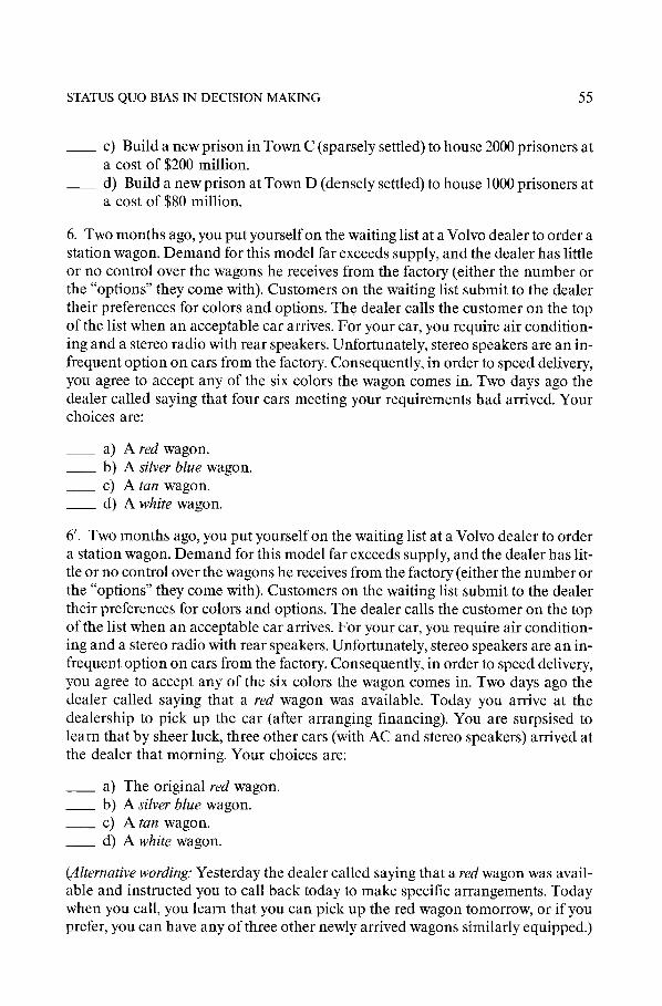
STATUS QUO BIAS IN DECISION MAKING 55
- c) Build a new prison in Town C (sparsely settled) to house 2000 prisoners at a cost of $200 million.
- d) Build a new prison at Town D (densely settled) to house 1000 prisoners at a cost of $80 million.
6. Two months ago, you put yourself on the waiting list at a Volvo dealer to order a station wagon. Demand for this model far exceeds supply, and the dealer has little or no control over the wagons he receives from the factory (either the number or the “options” they come with). Customers on the waiting list submit to the dealer their preferences for colors and options. The dealer calls the customer on the top of the list when an acceptable car arrives. For your car, you require air condition- ing and a stereo radio with rear speakers. Unfortunately, stereo speakers are an in- frequent option on cars from the factory. Consequently, in order to speed delivery, you agree to accept any of the six colors the wagon comes in. Two days ago the dealer called saying that four cars meeting your requirements had arrived. Your choices are:
~ a) A red wagon. __ b) A silver blue wagon. - c) A tan wagon. - d) A white wagon.
6’. Two months ago, you put yourself on the waiting list at a Volvo dealer to order a station wagon. Demand for this model far exceeds supply, and the dealer has lit- tle or no control over the wagons he receives from the factory (either the number or the “options” they come with). Customers on the waiting list submit to the dealer their preferences for colors and options. The dealer calls the customer on the top of the list when an acceptable car arrives. For your car, you require air condition- ing and a stereo radio with rear speakers. Unfortunately, stereo speakers are an in- frequent option on cars from the factory. Consequently, in order to speed delivery, you agree to accept any of the six colors the wagon comes in. Two days ago the dealer called saying that a red wagon was available. Today you arrive at the dealership to pick up the car (after arranging financing). You are surpsised to learn that by sheer luck, three other cars (with AC and stereo speakers) arrived at the dealer that morning. Your choices are:
- a) The original red wagon. ~ b) A silver blue wagon. - c) A tan wagon. - d) A white wagon.
(Alternative wording: Yesterday the dealer called saying that a red wagon was avail- able and instructed you to call back today to make specific arrangements. Today when you call, you learn that you can pick up the red wagon tomorrow, or if you prefer, you can have any of three other newly arrived wagons similarly equipped.)

56 WILLIAM SAMUELSON AND RICHARD ZECKHAUSER
7. Your first job as newly appointed water commissioner is to reassess the dis- tribution of water from a large auxiliary reservoir in the district. In three of the last ten years, drought conditions were so severe as to warrant drawing water from this reserve. Once again, the current year is marked by a prolonged drought. Two dis- tinct groups-agricultural growers and the residents of a nearby town-are clamoring for (and competing for) their share of the water. The 35,000 town residents are currently suffering under severe water rationing. For their part, the growers (operating some 120 farms) could lose between 20% and 60% of their out- put (depending upon the crop) without the extra water. Some 450,000 acre feet of water is available from the auxiliary reservoir. Unfortunately, the town’s demand for extra water is 260,000 acre feet, while the farmers say they need over 350,000 acre feet of extra water to limit their crop losses. Finally, you are also aware that during the last drought three years ago, the previous commissioner distributed 300,000 acre feet to the town and 150,000 acre feet to the farmers.
What is your distribution plan? (Check one of the plans below.)
0 acre feet to the town and 450,000 acre feet to the farmers.
- 50,000 acre feet to the town and 400,000 acre feet to the farmers.
__ lOO,OOO acre feet to the town and 350,000 acre feet to the farmers.
- 150,000 acre feet to the town and 300,000 acre feet to the farmers.
- 200,000 acre feet to the town and 250,000 acre feet to the farmers.
- 250,000 acre feet to the town and 200,000 acre feet to the farmers.
- 300,000 acre feet to the town and 150,000 acre feet to the farmers.
- 350,000 acre feet to the town and 100,000 acre feet to the farmers.
- 400,000 acre feet to the town and 50,000 acre feet to the farmers.
- 450,000 acre feet to the town and 0 acre feet to the farmers.
Version 2 of this question is the same as above except the allocations in the last line are: 200,000 acre feet to the town and 250,000 acre feet to the farmers.
Version 3 is the same as above except the allocations in the last line are: 100,000 acre feet to the town and 350,000 acre feet to the farmers.
8. You are the head of your own management consulting firm with a roster of three junior consultants and two support staff. You rent quarters in a small office building that is 15 minutes (in normal traffic) from your home, IO minutes from a cluster of clients on Route 128, and 30 minutes from the airport. Your current lease will be up shortly and you are considering moving to new quarters (having 10%

STATUS QUO BIAS IN DECISION MAKMG 57
more space) in a recently completed office complex. The new office is located 5 minutes from your home, 25 minutes from Route 128, and 20 minutes from the air- port. As an inducement to sign the new lease, your landlord-to-be has agreed to pay your company’s moving costs. You are aware that moving to the new quarters will mean an increase in your annual rental payment. How much more (than your current annual rental payment) would you be willing to pay for the new quarters? (At this price, you should be just indifferent between staying in your old quarters or moving to the new ones.) Check one of the alternatives below.
__ 0% to 10% higher - 11% to 20% higher - 21% to 30% higher
__ 31% to 40% higher __ 41% to 50% higher - more than 50% higher
Using your best judgment, write down the exact extra amount you would be willing to pay for the new space.
__ % more. (This amount should lie in the interval that you checked above.)
8’. You are the head of your own management consulting firm with a roster of three junior consultants and two support staff. You rent quarters in a new office complex that is 5 minutes (in normal traffic) from your home, 1.5 minutes from a cluster of clients on Route 128, and 20 minutes from the airport. Your current lease will be up shortly and you are considering moving to new quarters (having 10% less space) in a small, older office building. The new office is located 15 minutes from your home, 10 minutes from Route 128, and 30 minutes from the airport. As an inducement to sign the new lease, your landlord-to-be has agreed to pay your company’s moving costs. You are quite confident that you can acquire the space in the office building for a reduced annual rental payment. How much lower (relative to your current annual rental payment) would the new rent have to be for you to be willing to move to the new quarters? (At this price, you should be just indifferent between staying in your old quarters or moving to the new ones.) Check one of the alternatives below.
- 0% to 10% lower __ 11% to 20% lower ~ 21% to 30% lower
~ 31% to 40% lower __ 41% to 50% lower __ more than 50% lower
Using your best judgment, write down the exact amount you would be willing to pay for the new space.
__ % lower. (This amount should lie in the interval that you checked above.)
(Alternative wording: (For twenty-three subjects, the description in 8 and 8’ omitted the phrase, “As an inducement to sign the new lease, your landlord-to-be has agreed to pay your company’s moving costs.“)
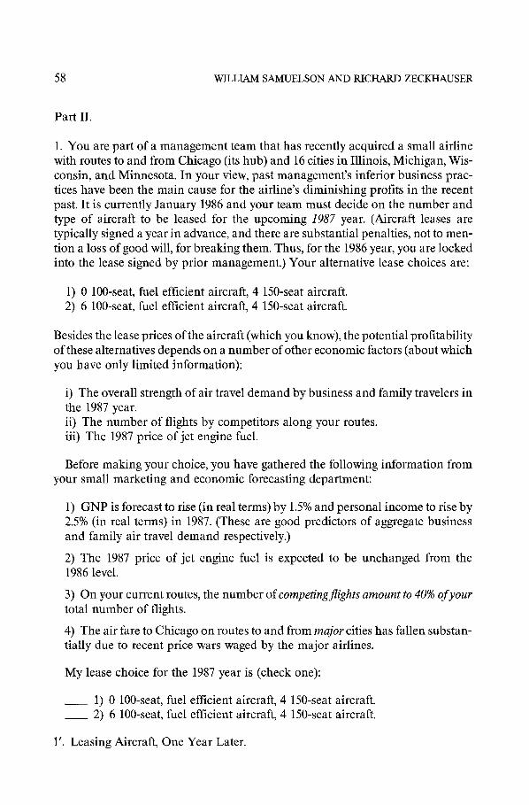
58 WILLIAM SAMUELSON AND RICHARD ZECKHAUSER
Part II.
1. You are part of a management team that has recently acquired a small airline with routes to and from Chicago (its hub) and 16 cities in Illinois, Michigan, Wis- consin, and Minnesota. In your view, past management’s inferior business prac- tices have been the main cause for the airline’s diminishing profits in the recent past. It is currently January 1986 and your team must decide on the number and type of aircraft to be leased for the upcoming 2987 year. (Aircraft leases are typically signed a year in advance, and there are substantial penalties, not to men- tion a loss of good will, for breaking them. Thus, for the 1986 year, you are locked into the lease signed by prior management.) Your alternative lease choices are:
1) 0 loo-seat, fuel efficient aircraft, 4 150-seat aircraft. 2) 6 loo-seat, fuel efficient aircraft, 4 150-seat aircraft.
Besides the lease prices of the aircraft (which you know), the potential profitability of these alternatives depends on a number of other economic factors (about which you have only limited information):
i) The overall strength of air travel demand by business and family travelers in the 1987 year. ii) The number of flights by competitors along your routes. iii) The 1987 price of jet engine fuel.
Before making your choice, you have gathered the following information from your small marketing and economic forecasting department:
1) GNP is forecast to rise (in real terms) by 1.5% and personal income to rise by 2.5% (in real terms) in 1987. (These are good predictors of aggregate business and family air travel demand respectively.)
2) The 1987 price of jet engine fuel is expected to be unchanged from the 1986 level.
3) On your current routes, the number of competing$ights amount to 40% ofyour total number of flights.
4) The air fare to Chicago on routes to and from major cities has fallen substan- tially due to recent price wars waged by the major airlines.
My lease choice for the 1987 year is (check one):
__ 1) 0 loo-seat, fuel efficient aircraft, 4 150-seat aircraft. __ 2) 6 loo-seat, fuel efficient aircraft, 4 150-seat aircraft.
1’. Leasing Aircraft, One Year Later.

STATUS QUO BIAS IN DECISION MAIGNG 59
Recall that your lease choice in question 1 was:
0 loo-seat, fuel efficient aircraj?, 4 150-seat aircraft.
It is now January 1987 and you must make your lease decision for the 1988 year. Your choices are the same as before. In addition to the previous information, you have the following new facts:
1) Over the past year, the airline has earned a modest profit, due (in your opi- nion) to your efforts to cut costs, revamp air routes, and lure back customers. Your prior forecasts of 1987 GNP and personal income appear to be about on target, though it is still too early to tell.
2) GNP is forecast to rise (in real terms) by 4.5% and personal income to rise by 4.0% (in real terms) in 1988.
3) The 1988 price of jet engine fuel is expected to be down slightly from the 1987 level.
4) On your current routes during the past year, the number of competing flights amounted to 50% of your total number of flights.
5) In recent months, the air fare to Chicago on routes to and from major cities has stayed at a high level due to the major airlines’ efforts to resist price wars.
My lease choice for the 1988 year is (check one):
- 1) Stick with 0 loo-seat, fuel efficient aircraft, 4 150-seat aircraft. __ 2) 6 loo-seat, fuel efficient aircraft, 0 150-seat aircraft.
END OF QUESTIONNAIRE
(Alternative wovding: There are no financial costs for changing your lease. The market for airline personnel, both pilots and flight attendants, is brisk. You can easily lay off or hire additional personnel. In addition to the previous information, you have the following new facts:
1) Over the past year, you have made effective efforts to cut costs, improve schedules, and provide quality service. Your prior forecasts appear to be on target, though it is still too early to tell.)