Statistics lecture 4

Relationships BetweenMeasurement Variables

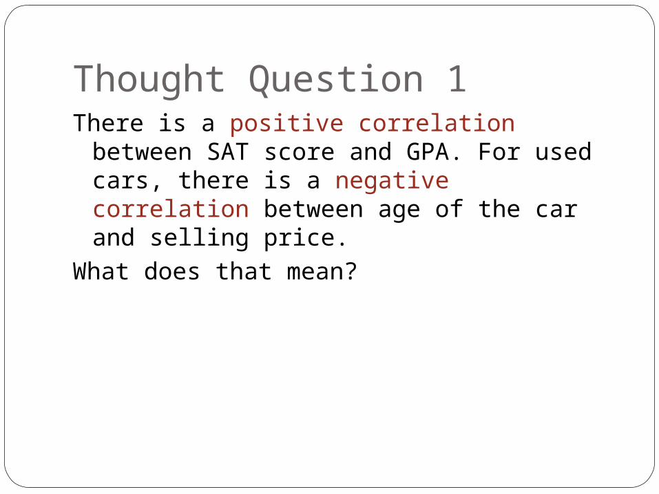
Thought Question 1There is a positive correlation between SAT

score and GPA. For used cars, there is a negative correlation between age of the car and selling price.

What does that mean?

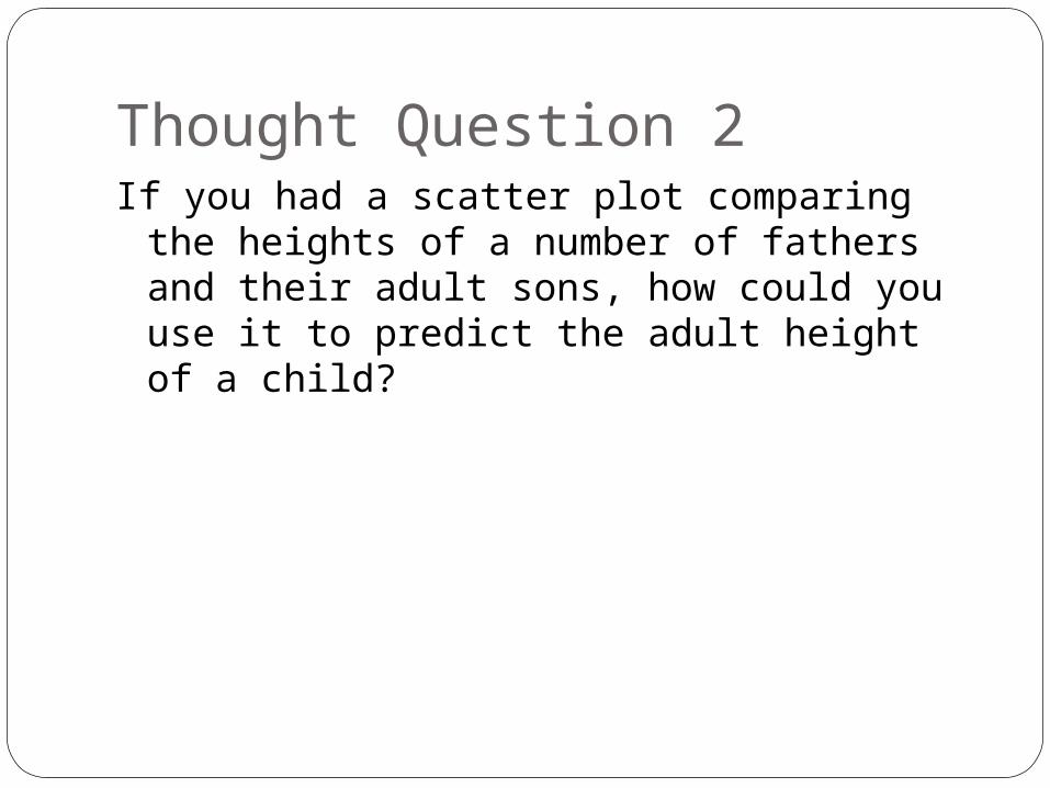
Thought Question 2If you had a scatter plot comparing the

heights of a number of fathers and their adult sons, how could you use it to predict the adult height of a child?

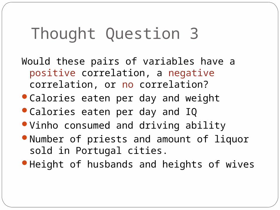
Thought Question 3

Would these pairs of variables have a positive correlation, a negative correlation, or no correlation?

Calories eaten per day and weightCalories eaten per day and IQVinho consumed and driving abilityNumber of priests and amount of liquor sold

in Portugal cities.Height of husbands and heights of wives

Goals for this lectureGet the idea of a statistical relationship and

statistical significanceUnderstand the meaning of correlation

between two measurement variablesLearn how to use the linear relationship

between two variables to predict one value, given the other

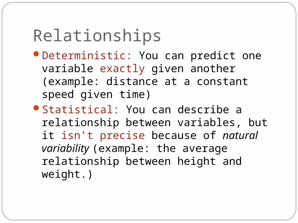
RelationshipsDeterministic: You can predict one variable

exactly given another (example: distance at a constant speed given time)

Statistical: You can describe a relationship between variables, but it isn’t precise because of natural variability (example: the average relationship between height and weight.)

Remember How to Build a Scatter Plot?

Doig

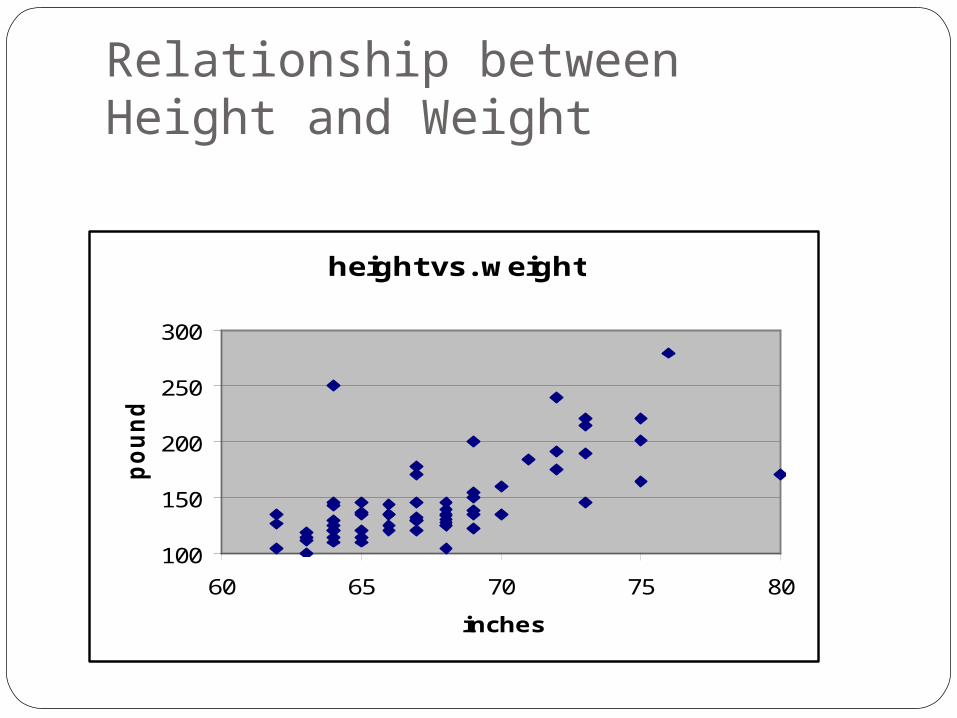
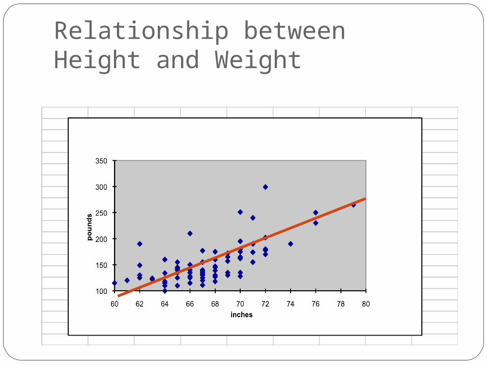
Relationship betweenHeight and Weight

height vs. weight

100

150

200

250

300

60 65 70 75 80

inches

po

un

ds

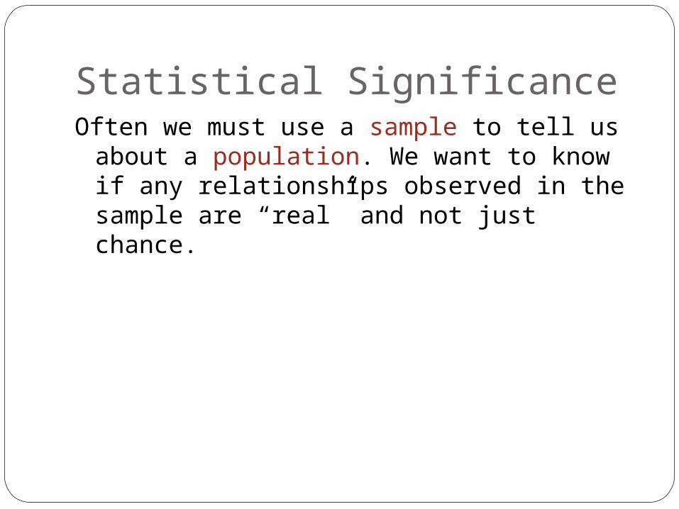
Statistical SignificanceOften we must use a sample to tell us about

a population. We want to know if any relationships observed in the sample are “real” and not just chance.

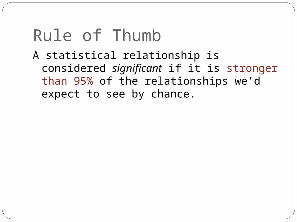
Rule of ThumbA statistical relationship is considered

significant if it is stronger than 95% of the relationships we’d expect to see by chance.

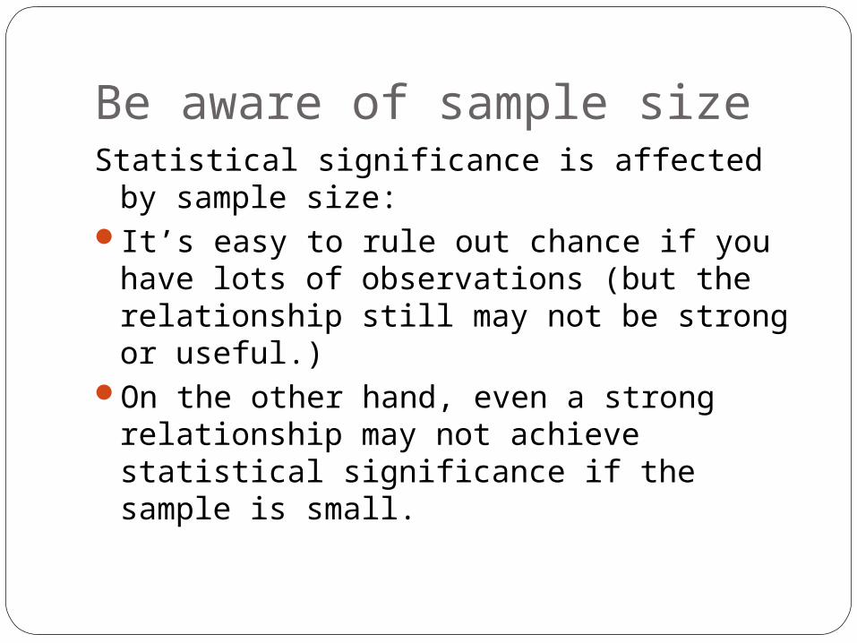
Be aware of sample sizeStatistical significance is affected by sample

size:It’s easy to rule out chance if you have lots

of observations (but the relationship still may not be strong or useful.)

On the other hand, even a strong relationship may not achieve statistical significance if the sample is small.

Relationship betweenHeight and Weight

Relationship betweenHeight and Weight

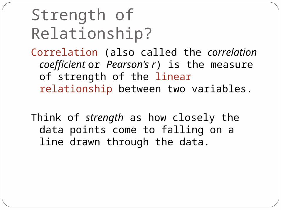
Strength of Relationship?Correlation (also called the correlation

coefficient or Pearson’s r) is the measure of strength of the linear relationship between two variables.

Think of strength as how closely the data points come to falling on a line drawn through the data.

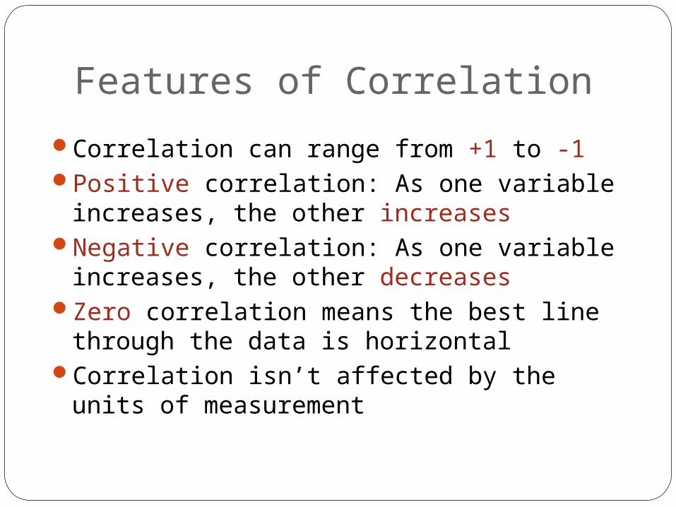
Features of Correlation

Correlation can range from +1 to -1Positive correlation: As one variable

increases, the other increasesNegative correlation: As one variable

increases, the other decreasesZero correlation means the best line

through the data is horizontalCorrelation isn’t affected by the units of

measurement

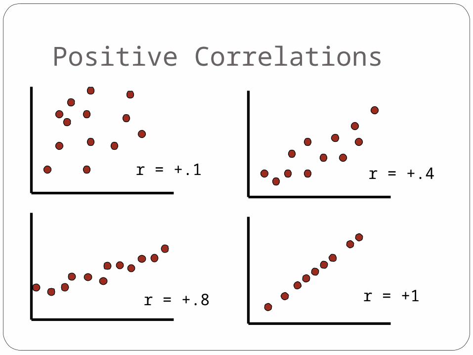
Positive Correlations

r = +.1 r = +.4

r = +.8 r = +1

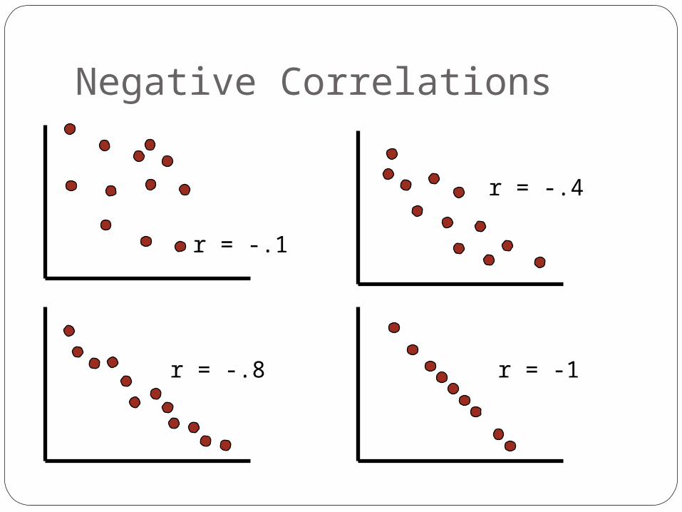
Negative Correlations

r = -.1

r = -.4

r = -.8 r = -1

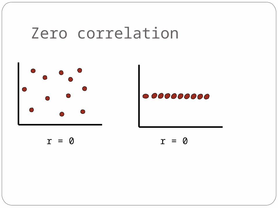
Zero correlation

r = 0 r = 0

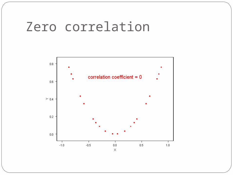
Zero correlation

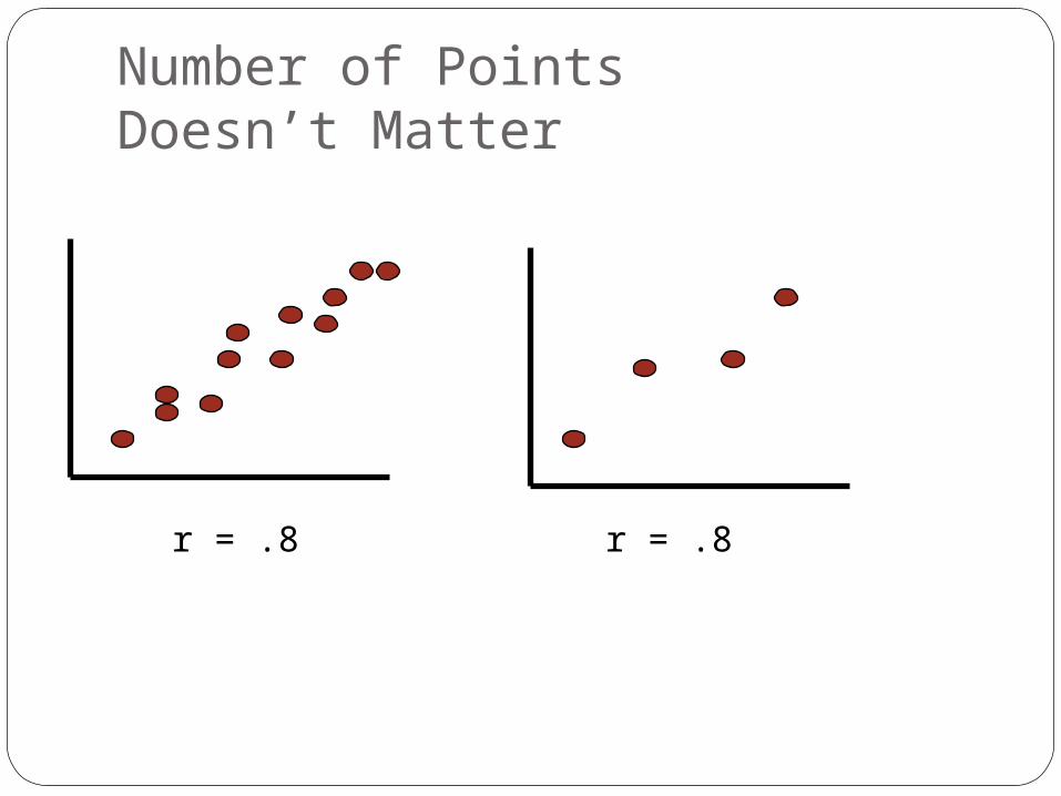
Number of PointsDoesn’t Matter

r = .8 r = .8

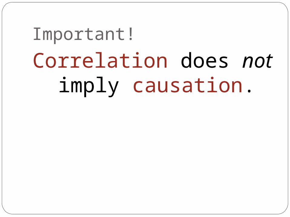
Important!

Correlation does not imply causation.

Linear RegressionIn addition to figuring the strength of the

relationship, we can create a simple equation that describes the best-fit line (also called the “least-squares” line) through the data.

This equation will help us predict one variable, given the other.

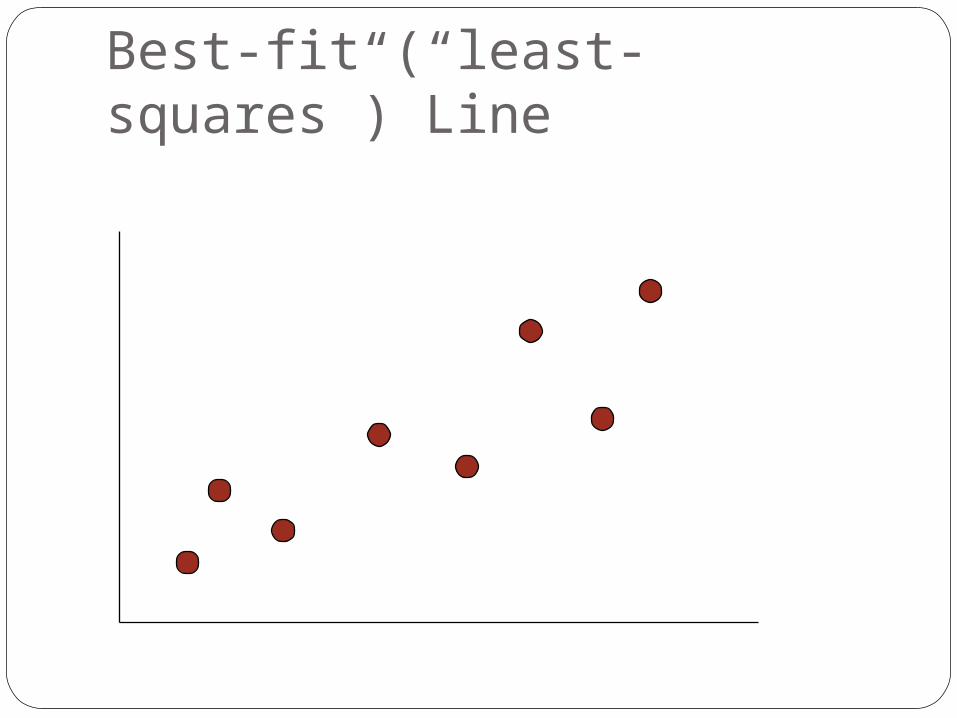
Best-fit (“least-squares”) Line

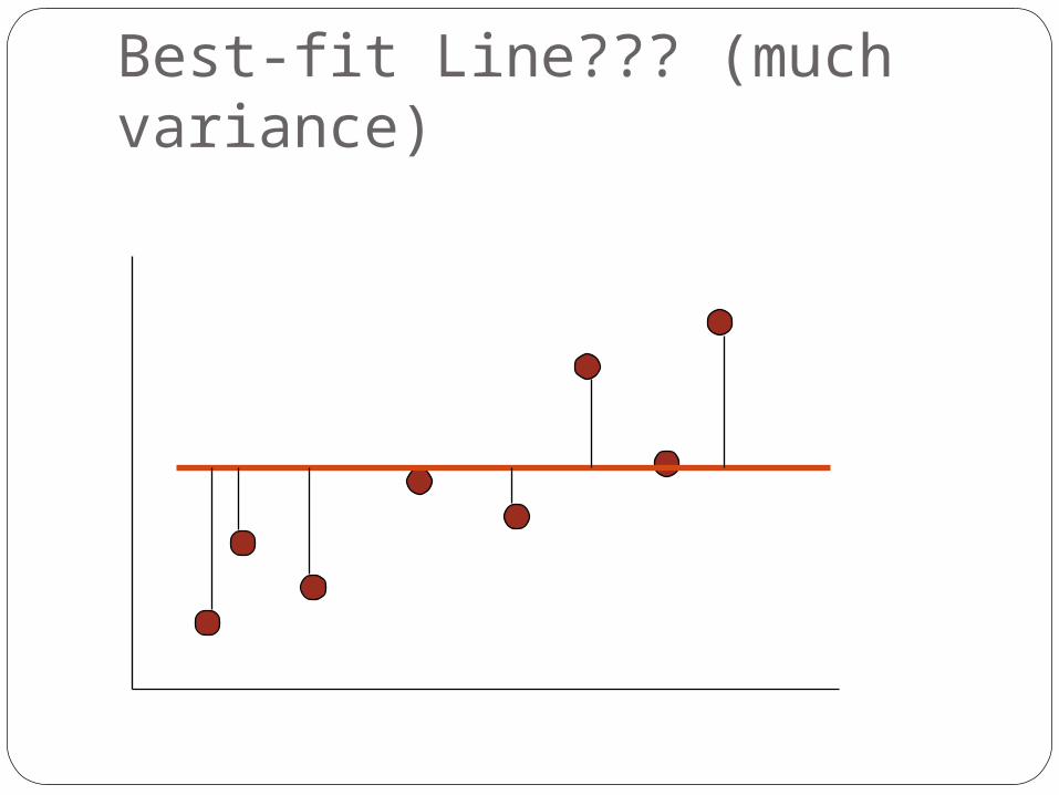
Best-fit Line??? (much variance)

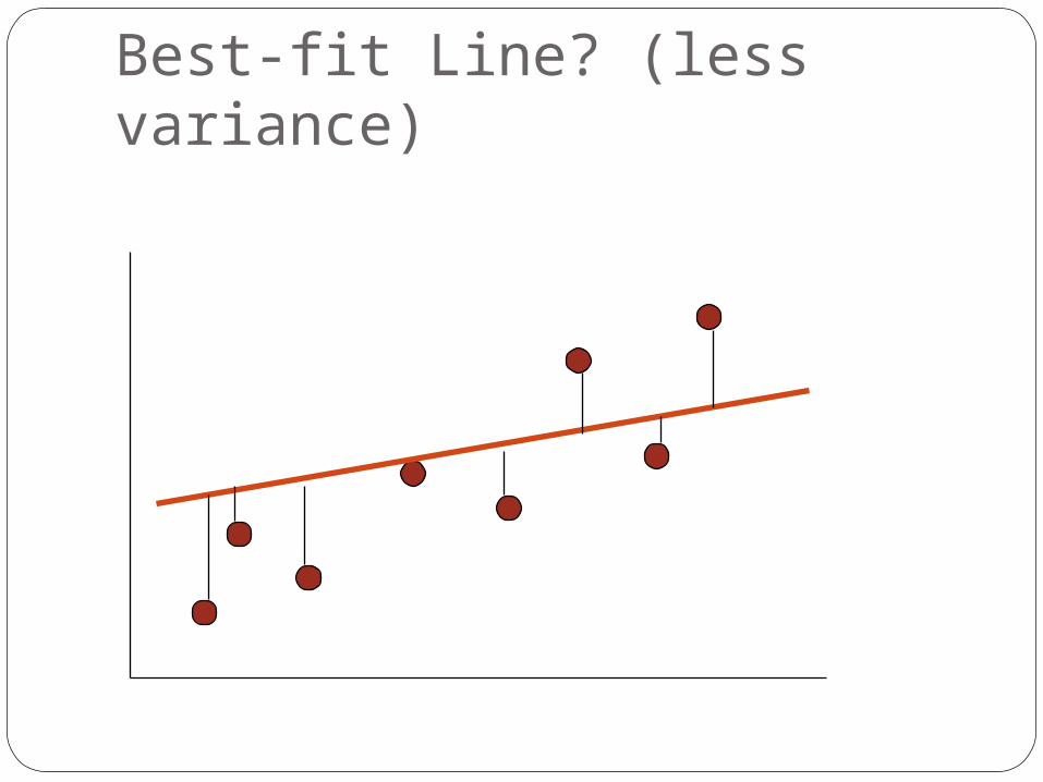
Best-fit Line? (less variance)

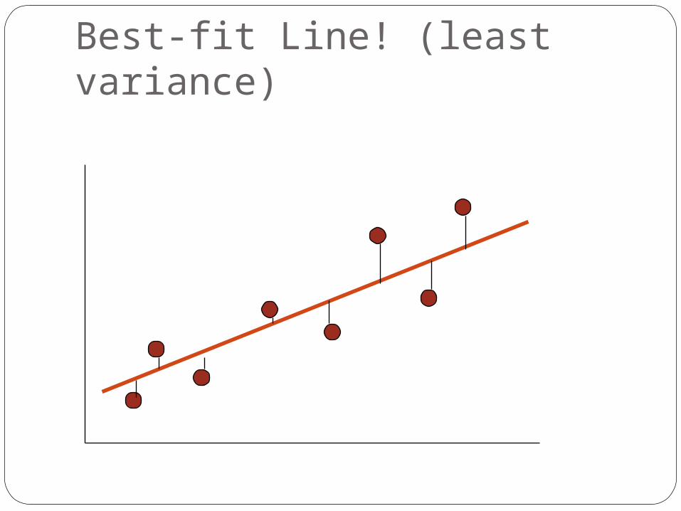
Best-fit Line! (least variance)

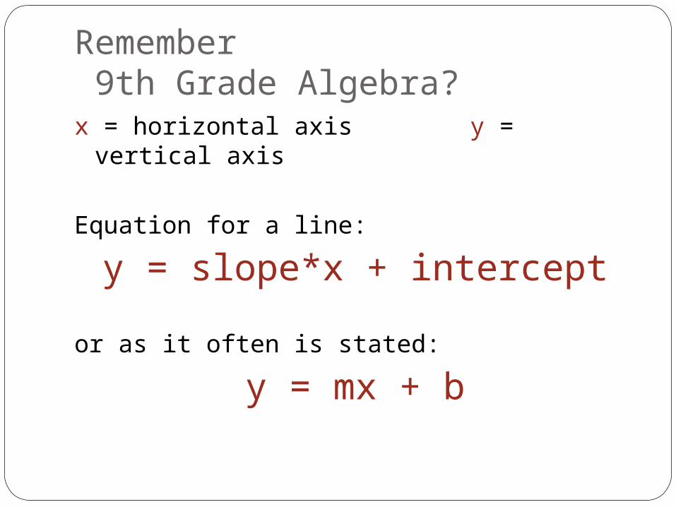
Remember 9th Grade Algebra?x = horizontal axis y = vertical axis

Equation for a line:

y = slope*x + intercept

or as it often is stated:

y = mx + b

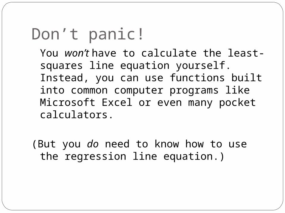
Don’t panic!You won’t have to calculate the least-squares line equation yourself. Instead, you can use functions built into common computer programs like Microsoft Excel or even many pocket calculators.

(But you do need to know how to use the regression line equation.)

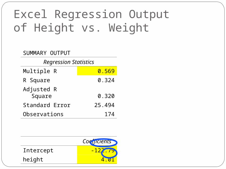
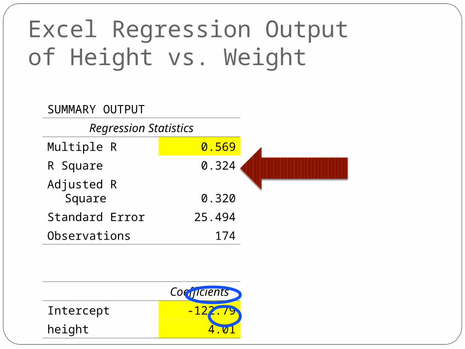
Excel Regression Outputof Height vs. Weight

SUMMARY OUTPUT

Regression Statistics

Multiple R 0.569

R Square 0.324

Adjusted R Square 0.320

Standard Error 25.494

Observations 174

  Coefficients

Intercept -122.79

height 4.01

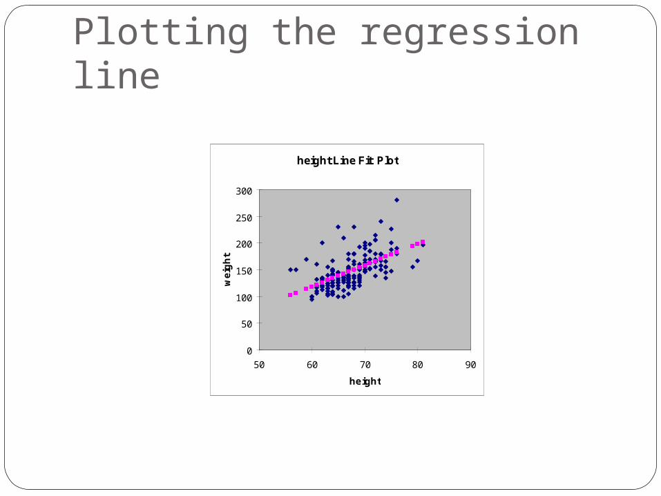
Plotting the regression line

height Line Fit Plot

0

50

100

150

200

250

300

50 60 70 80 90

height

we

igh

t

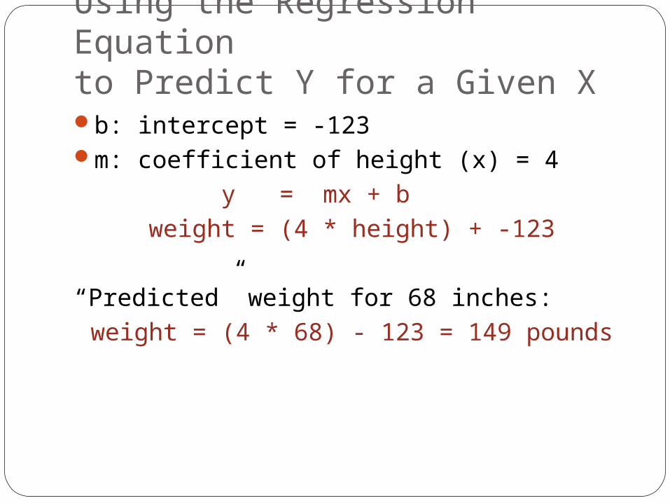
Using the Regression Equationto Predict Y for a Given Xb: intercept = -123m: coefficient of height (x) = 4

y = mx + b weight = (4 * height) + -123

“Predicted” weight for 68 inches: weight = (4 * 68) - 123 = 149 pounds

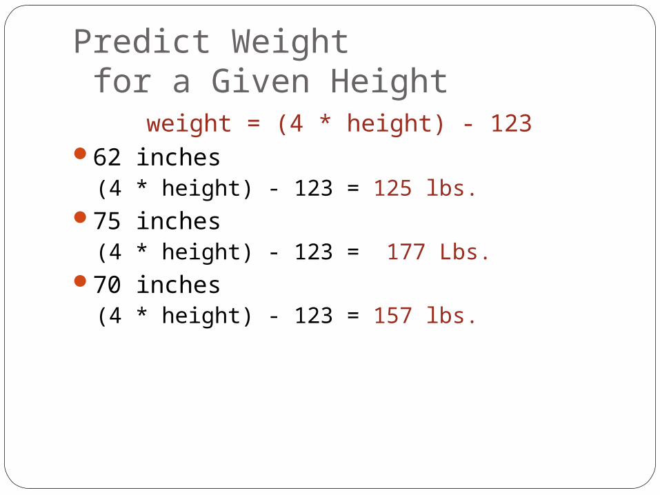
Predict Weight for a Given Height

weight = (4 * height) - 123 62 inches

(4 * height) - 123 = 125 lbs.75 inches

(4 * height) - 123 = 177 Lbs.70 inches

(4 * height) - 123 = 157 lbs.

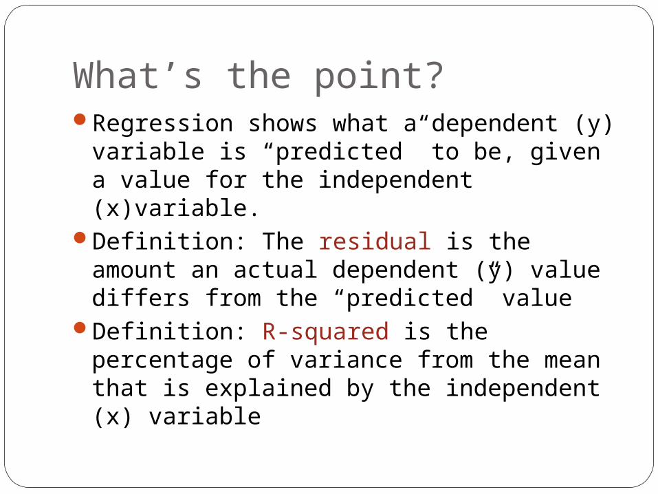
What’s the point?Regression shows what a dependent (y)

variable is “predicted” to be, given a value for the independent (x)variable.

Definition: The residual is the amount an actual dependent (y) value differs from the “predicted” value

Definition: R-squared is the percentage of variance from the mean that is explained by the independent (x) variable

Excel Regression Outputof Height vs. Weight

SUMMARY OUTPUT

Regression Statistics

Multiple R 0.569

R Square 0.324

Adjusted R Square 0.320

Standard Error 25.494

Observations 174

  Coefficients

Intercept -122.79

height 4.01

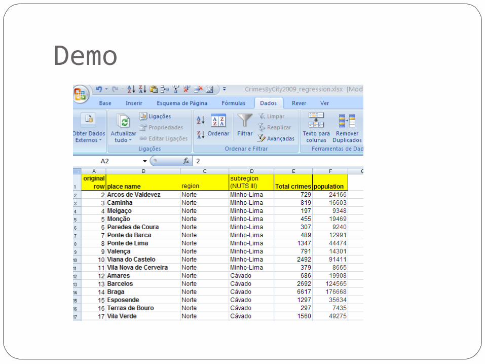
Demo

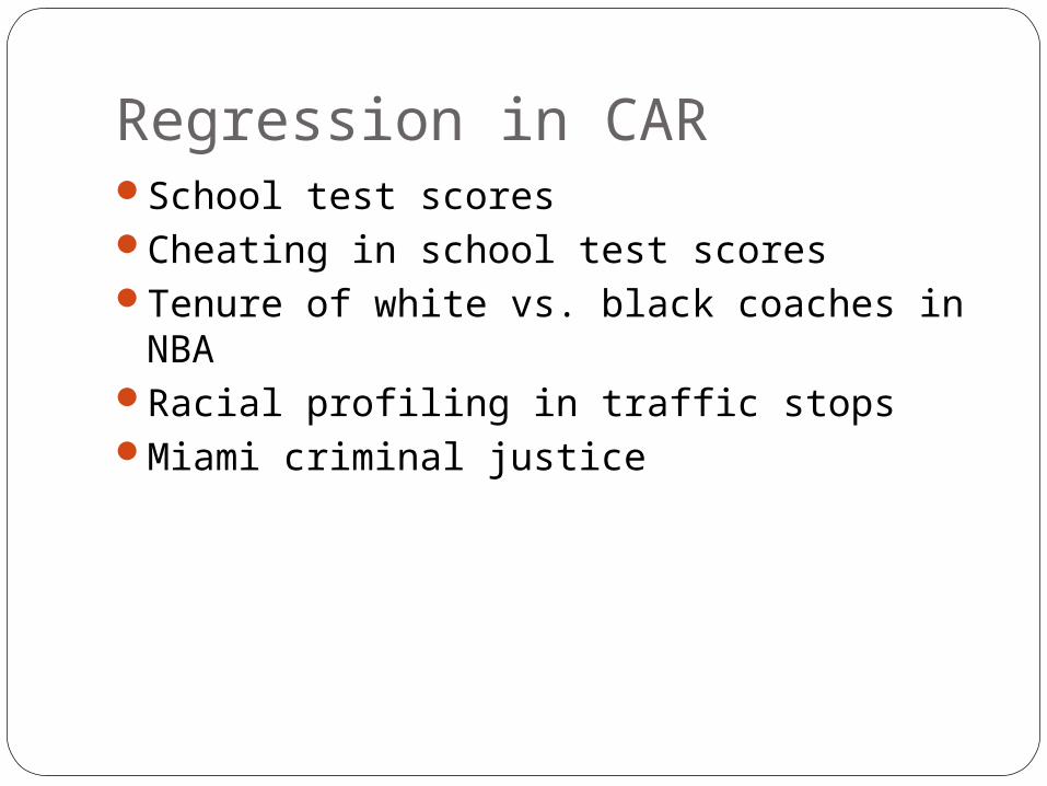
Regression in CARSchool test scoresCheating in school test scoresTenure of white vs. black coaches in NBARacial profiling in traffic stopsMiami criminal justice

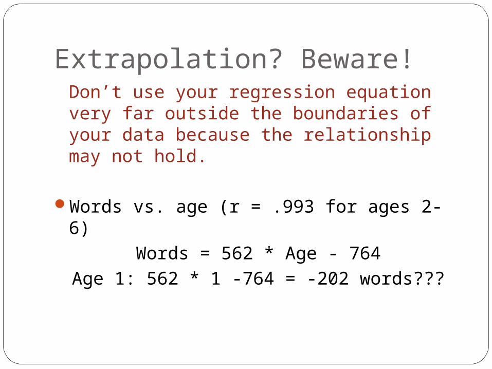
Extrapolation? Beware!Don’t use your regression equation very far outside the boundaries of your data because the relationship may not hold.

Words vs. age (r = .993 for ages 2-6)Words = 562 * Age - 764

Age 1: 562 * 1 -764 = -202 words???

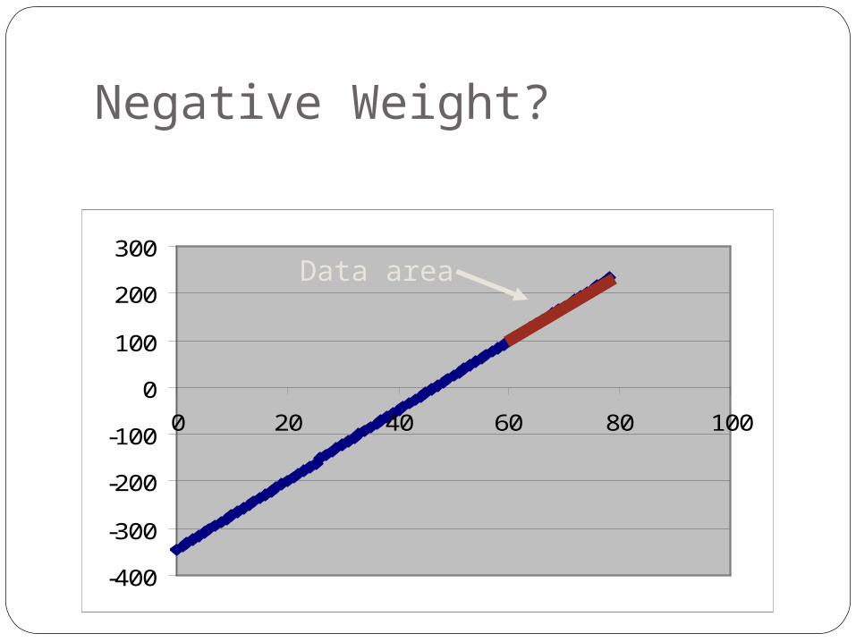
Negative Weight?

-400

-300

-200

-100

0

100

200

300

0 20 40 60 80 100

Data area

Mark Twain and the length of the Mississippi RiverFrom “Life on the Mississippi” (1884)In 176 years, the river was shortened by 403

kilometers, or about 2.3 kilometers per yearA million years ago, the Mississippi must

have been 2.2 million kilometers longIn 742 years, it will be 2.9 kilometers long,

joining Cairo, Illinois, and New OrleansTwain: “There is something fascinating about

science. One gets such wholesale returns of conjecture out of such a trifling investment of fact.”

Perguntas?