statistics 1 revision notes - wordpress.com · statistics 1 revision notes ... e.g. railway...

14/04/2013 Statistics 1 SDB 1

Statistics 1

Revision Notes

June 2012

2 14/04/2013 Statistics 1 SDB

Contents

1 Statistical modelling 6 Statistical modelling ............................................................................................................ 6

Definition ........................................................................................................................................................ 6 Advantages ..................................................................................................................................................... 6 Disadvantages ................................................................................................................................................. 6

2 Representation of sample data 7

Variables ............................................................................................................................. 7 Qualitative variables....................................................................................................................................... 7 Quantitative variables .................................................................................................................................... 7 Continuous variables ...................................................................................................................................... 7 Discrete variables ........................................................................................................................................... 7

Frequency distributions ....................................................................................................... 7 Frequency tables ............................................................................................................................................. 7 Cumulative frequency .................................................................................................................................... 7

Stem and leaf & back-to-back stem and leaf diagrams ....................................................... 8 Comparing two distributions from a back to back stem and leaf diagram. .................................................. 8

Grouped frequency distributions ......................................................................................... 8 Class boundaries and widths .......................................................................................................................... 8

Cumulative frequency curves for grouped data .................................................................. 9

Histograms .......................................................................................................................... 9

3 Mode, mean (and median) 11

Mode ................................................................................................................................. 11

Mean ................................................................................................................................. 11

Coding ............................................................................................................................... 12 Coding and calculating the mean ................................................................................................................. 12

Median .............................................................................................................................. 13

When to use mode, median and mean .............................................................................. 13 Mode ............................................................................................................................................................. 13 Median .......................................................................................................................................................... 13 Mean ............................................................................................................................................................. 13


4 Median (Q2), quartiles (Q1, Q3) and percentiles 14

Discrete lists and discrete frequency tables ...................................................................... 14 Interquartile range ........................................................................................................................................ 14 Discrete lists ................................................................................................................................................. 14 Discrete frequency tables ............................................................................................................................. 14

Grouped frequency tables, continuous and discrete data .................................................. 15 Grouped frequency tables, continuous data ................................................................................................. 15 Grouped frequency tables, discrete data ...................................................................................................... 16 Percentiles ..................................................................................................................................................... 17

Box Plots ........................................................................................................................... 17

Outliers ............................................................................................................................. 17

Skewness ........................................................................................................................... 18 Positive skew ................................................................................................................................................ 18 Negative skew .............................................................................................................................................. 19

5 Measures of spread 20

Range & interquartile range .............................................................................................. 20 Range ............................................................................................................................................................ 20 Interquartile range ........................................................................................................................................ 20

Variance and standard deviation ....................................................................................... 20 Proof of the alternative formula for variance .............................................................................................. 20 Rough checks, m ± s, m ± 2s ..................................................................................................................... 21 Coding and variance ..................................................................................................................................... 21

6 Probability 23

Relative frequency ............................................................................................................ 23

Sample spaces, events and equally likely outcomes ......................................................... 23

Probability rules and Venn diagrams ................................................................................ 23

Diagrams for two dice etc. ................................................................................................ 24

Tree diagrams ................................................................................................................... 25

Independent events ........................................................................................................... 26 To prove that A and B are independent ..................................................................................................... 26

Exclusive events ............................................................................................................... 27

Number of arrangements .................................................................................................. 27


7 Correlation 28

Scatter diagrams ................................................................................................................ 28 Positive, negative, no correlation & line of best fit. .................................................................................... 28

Product moment correlation coefficient, PMCC ............................................................. 28 Formulae ....................................................................................................................................................... 28 Coding and the PMCC ................................................................................................................................. 29 Interpretation of the PMCC ......................................................................................................................... 30

8 Regression 31

Explanatory and response variables .................................................................................. 31

Regression line .................................................................................................................. 31 Least squares regression line ....................................................................................................................... 31 Interpretation ................................................................................................................................................ 32

9 Discrete Random Variables 33

Random Variables ............................................................................................................. 33

Continuous and discrete random variables ....................................................................... 33 Continuous random variables ...................................................................................................................... 33 Discrete random variables ............................................................................................................................ 33

Probability distributions .................................................................................................... 33

Cumulative probability distribution .................................................................................. 34

Expectation or expected values ......................................................................................... 34 Expected mean or expected value of X. ....................................................................................................... 34 Expected value of a function ........................................................................................................................ 34 Expected variance ........................................................................................................................................ 34 Expectation algebra ...................................................................................................................................... 35

The discrete uniform distribution ...................................................................................... 36 Conditions for a discrete uniform distribution ............................................................................................ 36 Expected mean and variance ........................................................................................................................ 36 Non-standard uniform distribution .............................................................................................................. 37

10 The Normal Distribution N(μ, σ2) 38

The standard normal distribution N(0, 12) ...................................................................... 38

The general normal distribution N(μ, σ2) ....................................................................... 39 Use of tables ................................................................................................................................................. 39


11 Context questions and answers 42

Accuracy ........................................................................................................................... 42

Statistical models .............................................................................................................. 42

Histograms ........................................................................................................................ 43

Averages ........................................................................................................................... 43

Skewness ........................................................................................................................... 44

Correlation ........................................................................................................................ 45

Regression ......................................................................................................................... 46

Discrete uniform distribution ............................................................................................ 47

Normal distribution ........................................................................................................... 47

12 Appendix 49

–1 ≤ P.M.C.C. ≤ 1 ........................................................................................................... 49 Cauchy-Schwartz inequality ........................................................................................................................ 49 P.M.C.C. between –1 and +1 ....................................................................................................................... 49

Regression line and coding ............................................................................................... 50 Proof ............................................................................................................................................................. 50

Normal Distribution, Z = ......................................................................................... 51


1 Statistical modelling

Statistical modelling

Example: When a die is rolled, we say that the probability of each number is . This is a statistical model, but the assumption that each face is equally likely might not be true.

Suppose the die is weighted to increase the chance of a six. We might then find, after experimenting, that the probability of a six is and the probability of a one is , with the

probability of other faces remaining at . In this case we have refined, or improved, the model to give a truer picture.

Example: The heights of a large group of adults are measured. The mean is 172⋅3 cm and the standard deviation is 12⋅4 cm.

It is thought that the general shape of the histogram can be modelled by the curve

f (x) = · √

·

This might not give a true picture, in which case we would have to change the equation, or refine the model.

Definition A statistical model is a simplification of a real world situation. It can be used to make predictions about a real world problem. By analysing and refining the model an improved understanding may be obtained.

Advantages • the model is quick and easy to produce • the model helps our understanding of the real world problem • the model helps us to make predictions • the model helps us to control a situation – e.g. railway timetables, air traffic control etc.

Disadvantages • the model simplifies the situation and only describes a part of the real world problem. • the model may only work in certain situations, or for a particular range of values.


2 Representation of sample data

Variables

Qualitative variables Non-numerical - e.g. red, blue or long, short etc.

Quantitative variables Numerical - e.g. length, age, time, number of coins in pocket, etc

Continuous variables Can take any value within a given range - e.g. height, time, age etc.

Discrete variables Can only take certain values - e.g. shoe size, cost in £ and p, number of coins.

Frequency distributions

Frequency tables A list of discrete values and their frequencies.

Example: The number of M&M s is counted in several bags, and recorded in the frequency table below:

number of M&M s 37 38 39 40 41 42 43

frequency 3 8 11 19 13 7 2

Cumulative frequency Add up the frequencies as you go down the list

number of M&M s 37 38 39 40 41 42 43

frequency 3 8 11 19 13 7 2

cumulative frequency 3 11 22 41 54 61 63


Stem and leaf & back-to-back stem and leaf diagrams

Line up the digits on the leaves so that it looks like a bar chart. Add a key; e.g. 5|2 means 52, or 4|3 means 4⋅3 etc.

Comparing two distributions from a back to back stem and leaf diagram.

A B 8/1 = 81 8 1 2 2 4 5 6 7 8

3 1 0 7 2 3 5 6 7 7 8 8 9 9 9 3 2 2 1 1 6 1 3 4 5 5 6 6 7 8 8 8 9 9

7 6 5 5 3 3 5 0 0 1 2 3 4 5 6 8 9 8 7 4 3 0 0 4

8 7 5 3 1 1 3 9 9 7 4 2 2 5 4 3 2 1 1

8 7 0

1. The values in A are on average smaller than those in B 2. The values in A are more spread out than those in B.

Grouped frequency distributions

Class boundaries and widths When deciding class boundaries you must not leave a gap between one class and another, whether dealing with continuous or discrete distributions. For discrete distributions avoid leaving gaps between classes by using class boundaries as shown below: X 0, 1, 2, 3, 4, 5, 6, 7, …

Class interval – as given

Class contains

Class boundaries without gaps

0 – 4 0, 1, 2, 3, 4 0 – 4

5 – 9 5, 6, 7, 8, 9 4 – 9

10 – 12 10, 11, 12 9 – 12

etc

For continuous distributions the class boundaries can be anywhere.


Cumulative frequency curves for grouped data

class

interval class

boundaries frequency class cumulative frequency

0 - 4 0 to 4 ½ 27 ≤ 4 ½ 27

5 – 9 4 ½ to 9 ½ 36 ≤ 9 ½ 63

10 – 19 9 ½ to 19 ½ 54 ≤ 19 ½ 117

20 – 29 19 ½ to 29 ½ 49 ≤ 29 ½ 166

30 – 59 29 ½ to 59 ½ 24 ≤ 59 ½ 190

60 –99 59 ½ to 99 ½ 10 ≤ 99 ½ 200

Plot points at ends of intervals, (4 , 27), (9 , 63), (19 , 117) etc. and join points with a

smooth curve.

Histograms

Plot the axes with a continuous scale as normal graphs.

There are no gaps between the bars of a histogram.

Area equals frequency.

Note that the total area under a frequency histogram is N, the total number

and the area from a to b is the number of items between a and b.

To draw a histogram, first draw up a table showing the class intervals, class boundaries, class

widths, frequencies and then heights = – as shown below:

class interval

class boundaries

class width frequency height

0 - 4 0 to 4 4 27 6

5 – 9 4 to 9 5 36 7⋅2

10 – 19 9 to 19 10 54 5⋅4

20 – 29 19 to 29 10 49 4⋅9

30 – 59 29 to 59 30 24 0⋅8


60 –99 59 to 99 40 10 0⋅25

Example: A grouped frequency table for the weights of adults has the following entries:

weight kg … … 50 – 60 … 70 – 85 …

frequency … … 60 … 20 …

In a histogram, the bar for the class 50 – 60 kg is 2 cm wide and 9 cm high.

Find the width and height of the bar for the 70 – 85 kg class.

Solution: 50 – 60 is usually taken to mean 50 ≤ weight < 60

The width of the 50 – 60 class is 10 kg ≡ 2 cm

⇒ width of the 70 – 85 class is 15 kg ≡ × 2 = 3 cm

The area of the 50 – 60 bar is 2 × 9 = 18 cm2 ≡ frequency 60

⇒ the frequency of the 70 – 85 bar is 20 ≡ an area of × 18 = 6 cm2

⇒ the height of the 70 – 85 bar is area ÷ width = 6 ÷ 3 = 2 cm.

Answer width of 70 – 85 kg bar is 3 cm, and height is 2 cm.


3 Mode, mean (and median)

Mode The mode is the value, or class interval, which occurs most often.

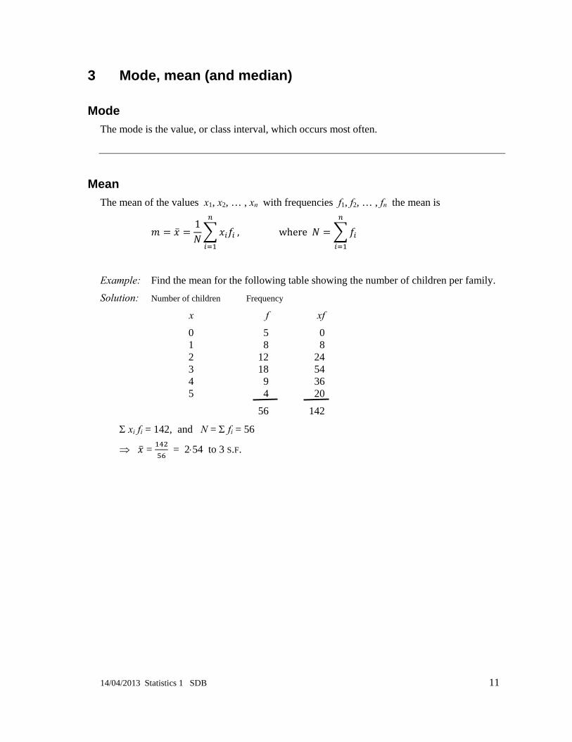
Mean The mean of the values x1, x2, … , xn with frequencies f1, f2, … , fn the mean is

1, where

Example: Find the mean for the following table showing the number of children per family.

Solution: Number of children Frequency

x f xf

0 5 0 1 8 8 2 12 24 3 18 54 4 9 36 5 4 20

56 142

Σ xi fi = 142, and N = Σ fi = 56

⇒ = = 2⋅54 to 3 S.F.


In a grouped frequency table you must use the mid-interval value. Example: The table shows the numbers of children in prep school classes in a town. Solution: Number Mid-interval Frequency

of children value

x f xf

1 - 10 5⋅5 5 27⋅5 11 - 15 13 8 104 16 – 20 18 12 216 21 - 30 25⋅5 18 459 31 - 40 35⋅5 11 390⋅5

54 1197 Σ xi fi = 1197, and N = Σ fi = 54

⇒ = = 22⋅2 to 3 S.F.

Coding

The weights of a group of people are given as x1, x2, … xn in kilograms. These weights are now changed to grammes and given as t1, t2, … tn .

In this case ti = 1000 × xi – this is an example of coding.

Another example of coding could be ti = 20

.

Coding and calculating the mean

With the coding, ti = 20

, we are subtracting 20 from each x-value and then dividing the result by 5.

We first find the mean for ti, and then we reverse the process to find the mean for xi ⇒ we find the mean for ti, multiply by 5 and add 20, giving = 5 + 20

Proof: ti = 20

⇒ xi = 5ti + 20

1

15 20

5

20


5 20 since 1

and

Example: Use the coding ti = 165

to find the mean weight for the following distribution.

Weight, kg Mid-interval Coded value Frequency

xi ti = 165

fi ti fi

140 - 150 145 –2 9 –18 150 - 160 155 –1 21 –21 160 - 170 165 0 37 0 170 - 180 175 1 28 28 180 - 190 185 2 11 22

106 11

⇒ =

and ti = 165 ⇒ = 10 + 165 = 10 × + 165 = 166⋅0377358

⇒ mean weight is 166⋅04 kg to 2 D.P. Here the coding simplified the arithmetic for those who like to work without a calculator!

Median

The median is the middle number in an ordered list. Finding the median is explained in the next section.

When to use mode, median and mean

Mode You should use the mode if the data is qualitative (colour etc.) or if quantitative (numbers) with a clearly defined mode (or bi-modal). It is not much use if the distribution is fairly even.

Median You should use this for quantitative data (numbers), particularly when there are extreme values (outliers).

Mean This is for quantitative data (numbers), and uses all pieces of data. It gives a true measure, but is affected by extreme values (outliers).


4 Median (Q2), quartiles (Q1, Q3) and percentiles

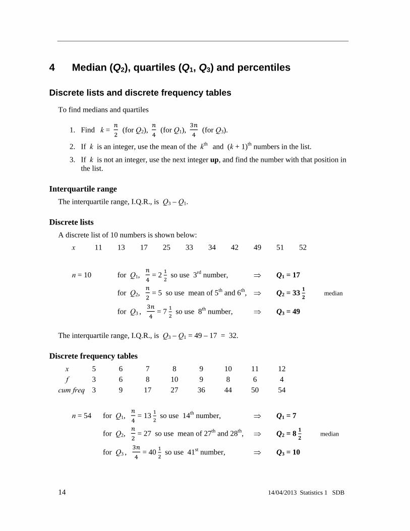
Discrete lists and discrete frequency tables

To find medians and quartiles

1. Find k = (for Q2), (for Q1), (for Q3).

2. If k is an integer, use the mean of the kth and (k + 1)th numbers in the list.

3. If k is not an integer, use the next integer up, and find the number with that position in the list.

Interquartile range The interquartile range, I.Q.R., is Q3 – Q1.

Discrete lists A discrete list of 10 numbers is shown below:

x 11 13 17 25 33 34 42 49 51 52

n = 10 for Q1, = 2 so use 3rd number, ⇒ Q1 = 17

for Q2, = 5 so use mean of 5th and 6th, ⇒ Q2 = 33 median

for Q3 , = 7 so use 8th number, ⇒ Q3 = 49

The interquartile range, I.Q.R., is Q3 – Q1 = 49 – 17 = 32.

Discrete frequency tables x 5 6 7 8 9 10 11 12 f 3 6 8 10 9 8 6 4 cum freq 3 9 17 27 36 44 50 54

n = 54 for Q1, = 13 so use 14th number, ⇒ Q1 = 7

for Q2, = 27 so use mean of 27th and 28th, ⇒ Q2 = 8 median

for Q3 , = 40 so use 41st number, ⇒ Q3 = 10


The interquartile range, I.Q.R., is Q3 – Q1 = 10 – 7 = 3.

Grouped frequency tables, continuous and discrete data

To find medians and quartiles

1. Find k = (for Q2), (for Q1), (for Q3). 2. Do not round k up or change it in any way. 3. Use linear interpolation to find median and quartiles – note that you must use the

correct intervals for discrete data (start at the s).

Grouped frequency tables, continuous data

class boundaries frequency cumulative frequency

0 ≤ x < 5 27 27 5 to 10 36 63 10 to 20 54 117 20 to 30 49 166 30 to 60 24 190 60 to 100 12 202

With continuous data, the end of one interval is the same as the start of the next – no gaps.

To find Q1, n = 202 ⇒ = 50 do not change it

From the diagram ⇒ Q1 = 5 + 5 × = 8⋅263888889 = 8⋅26 to 3 S.F.

5 Q1 10

27 50⋅5 63

23⋅5

36

Q1 – 5

5

class boundaries

cumulative frequencies


To find Q2, n = 202 ⇒ = 101 do not change it

From the diagram ⇒ Q2 = 10 + 10 × = 17⋅037…= 17⋅0 to 3 S.F.

Similarly for Q3, = 151⋅5, so Q3 lies in the interval (20, 30)

⇒ . ⇒ Q3 = 20 + 10 × .

= 27⋅0408… = 27⋅0 to 3 S.F.

Grouped frequency tables, discrete data The discrete data in grouped frequency tables is treated as continuous.

1. Change the class boundaries to the 4 , 9 etc. 2. Proceed as for grouped frequency tables for continuous data.

class interval

class boundaries frequency cumulative

frequency 0 – 4 0 to 4 ½ 25 25

5 – 9 4 ½ to 9 ½ 32 57

10 – 19 9 ½ to 19 ½ 51 108

20 – 29 19 ½ to 29 ½ 47 155

30 – 59 29 ½ to 59 ½ 20 175

60 –99 59 ½ to 99 ½ 8 183

To find Q1, n = 183 ⇒ = 45⋅75

From the diagram ·

10 Q2 20

63 101 117

class boundaries


4⋅5 Q1 9⋅5

25 45⋅75 57

class boundaries



⇒ Q1 = 4⋅5 + 5 × = 7⋅7421875…= 7⋅74 to 3 S.F. Q2 and Q3 can be found in a similar way.

Percentiles Percentiles are calculated in exactly the same way as quartiles. Example: For the 90th percentile, find and proceed as above.

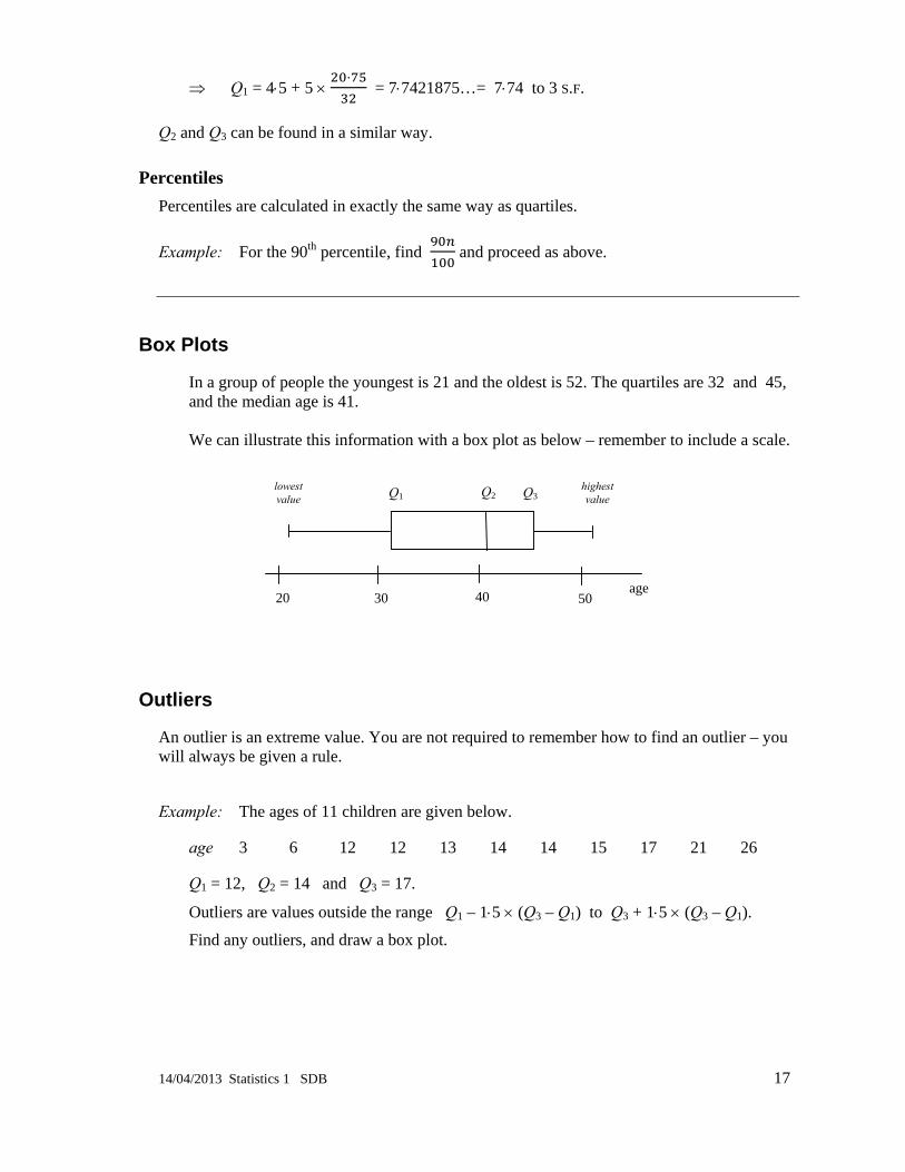
Box Plots

In a group of people the youngest is 21 and the oldest is 52. The quartiles are 32 and 45, and the median age is 41. We can illustrate this information with a box plot as below – remember to include a scale.

Outliers

An outlier is an extreme value. You are not required to remember how to find an outlier – you will always be given a rule.

Example: The ages of 11 children are given below.

age 3 6 12 12 13 14 14 15 17 21 26

Q1 = 12, Q2 = 14 and Q3 = 17.

Outliers are values outside the range Q1 – 1⋅5 × (Q3 – Q1) to Q3 + 1⋅5 × (Q3 – Q1).

Find any outliers, and draw a box plot.

lowest value

highestvalue Q3 Q1 Q2

20 30 40 50 age


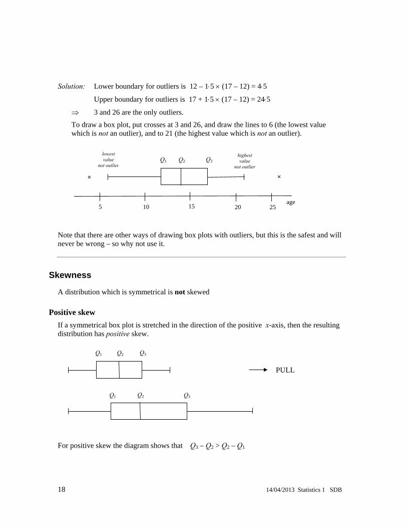
Solution: Lower boundary for outliers is 12 – 1⋅5 × (17 – 12) = 4⋅5

Upper boundary for outliers is 17 + 1⋅5 × (17 – 12) = 24⋅5

⇒ 3 and 26 are the only outliers.

To draw a box plot, put crosses at 3 and 26, and draw the lines to 6 (the lowest value which is not an outlier), and to 21 (the highest value which is not an outlier).

Note that there are other ways of drawing box plots with outliers, but this is the safest and will never be wrong – so why not use it.

Skewness

A distribution which is symmetrical is not skewed

Positive skew If a symmetrical box plot is stretched in the direction of the positive x-axis, then the resulting distribution has positive skew.

For positive skew the diagram shows that Q3 – Q2 > Q2 – Q1

Q3 Q1 Q2

Q3 Q1 Q2

PULL

lowest value

not outlier

highestvalue

not outlierQ3 Q1 Q2

5 10 15 20 age

25

× ×


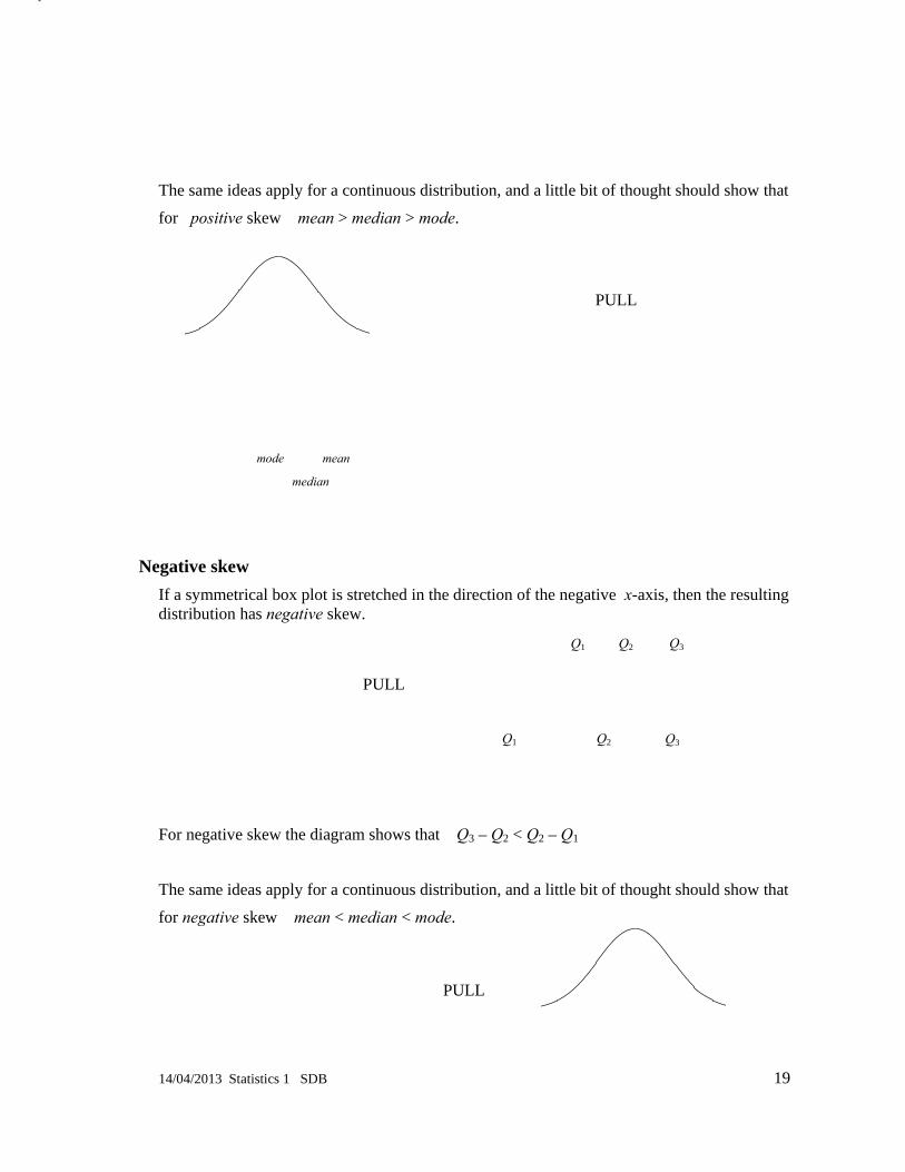
The same ideas apply for a continuous distribution, and a little bit of thought should show that

for positive skew mean > median > mode.

Negative skew If a symmetrical box plot is stretched in the direction of the negative x-axis, then the resulting distribution has negative skew.

For negative skew the diagram shows that Q3 – Q2 < Q2 – Q1

The same ideas apply for a continuous distribution, and a little bit of thought should show that

for negative skew mean < median < mode.

PULL

mode

median

mean

PULL

Q3 Q1 Q2

PULL

Q3 Q1 Q2


5 Measures of spread Range & interquartile range

Range The range is found by subtracting the smallest value from the largest value.

Interquartile range The interquartile range is found by subtracting the lower quartile from the upper quartile, so I.Q.R. = Q3 – Q1.

Variance and standard deviation

Variance is the square of the standard deviation.

1

, or

1

.

When finding the variance, it is nearly always easier to use the second formula. Variance and standard deviation measure the spread of the distribution.

Proof of the alternative formula for variance

1

1

2

1 1

2 1

1 2

since = ∑ and N = ∑

modemedian

mean


12

1

Rough checks, m ± s, m ± 2s When calculating a standard deviation, you should check that there is approximately

65 - 70% of the population within 1 s.d. of the mean and

approximately 95% within 2 s.d. of the mean.

These approximations are best for a fairly symmetrical distribution.

Coding and variance

Using the coding ti = we see that

xi = ati + k ⇒ = a + k

1

1

1

Notice that subtracting k has no effect, since this is equivalent to translating the graph, and therefore does not change the spread, and if all the x-values are divided by a, then we need to multiply st by a to find sx.

Example: Find the mean and standard deviation for the following distribution. Here the x-values are nasty, but if we change them to form ti = then the arithmetic in the last two columns becomes much easier.

x ti = f ti fi ti 2 fi

200 –2 12 –24 48 205 –1 23 –23 23 210 0 42 0 0 215 1 30 30 30 220 2 10 20 40

117 3 141 the mean of t is = ∑ = =


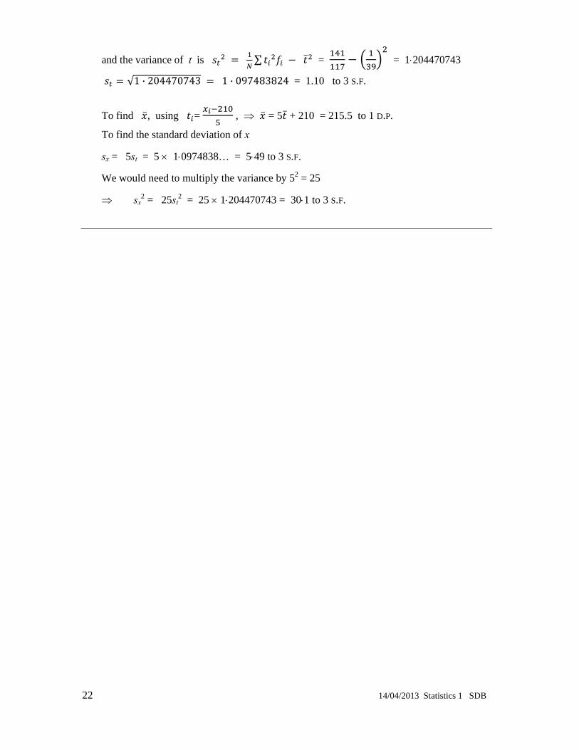
and the variance of t is ∑ = = 1⋅204470743

√1 · 204470743 1 · 097483824 = 1.10 to 3 S.F.

To find , using = , ⇒ = 5 + 210 = 215.5 to 1 D.P.

To find the standard deviation of x

sx = 5st = 5 × 1⋅0974838… = 5⋅49 to 3 S.F.

We would need to multiply the variance by 52 = 25

⇒ sx2 = 25st

2 = 25 × 1⋅204470743 = 30⋅1 to 3 S.F.


6 Probability Relative frequency

After tossing a drawing pin a large number of times the relative frequency of it landing point up is

;

this can be thought of as the experimental probability.

Sample spaces, events and equally likely outcomes

A sample space is the set of all possible outcomes, all equally likely. An event is a set of possible outcomes.

P(A) = NAnA )(

spacesampleinnumbertotalhappencanwaysofnumber

= , where N is number in sample space.

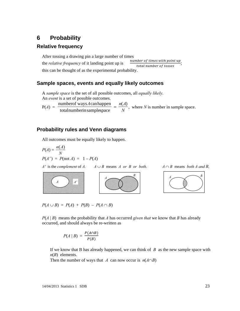
Probability rules and Venn diagrams

All outcomes must be equally likely to happen.

P(A) = NAn )(

P(A′ ) = P(not A) = 1 – P(A)

A′ is the complement of A. A ∪ B means A or B or both. A ∩ B means both A and B,

P(A ∪ B) = P(A) + P(B) – P(A ∩ B)

P(A | B) means the probability that A has occurred given that we know that B has already occurred, and should always be re-written as

P(A | B) =

If we know that B has already happened, we can think of B as the new sample space with n(B) elements. Then the number of ways that A can now occur is n(A∩B)

AB

A A′ A B


⇒ P(A | B) =

Diagrams for two dice etc.

When considering two dice, two spinners or a coin and a die, the following types of diagram are often useful – they ensure that all outcomes are equally likely to happen.

Two dice Coin and die Two coins Three coins green

6 × × × × × × 6 × × H H H H H 5 × × × × × × 5 × × H T H H T 4 × × × × × × 4 × × T H H T H 3 × × × × × × 3 × × T T T H H 2 × × × × × × 2 × × H T T 1 × × × × × × 1 × × T H T 1 2 3 4 5 6 red H T T T H T T T

From these diagrams it should be easy to see that

For two dice: P(total 10) = , P(red > green) = , P(total 10⏐4 on green) =

= .

For coin and die: P(Head and an even number) = .

For three dice: P(exactly two Heads) = .


Tree diagrams

The rules for tree diagrams are

Select which branches you need

Multiply along each branch

Add the results of each branch needed. Make sure that you include enough working to show which branches you are using (method).

Be careful to allow for selection with and without replacement.

Example: In the launch of a rocket, the probability of an electrical fault is 0⋅2. If there is an electrical fault the probability that the rocket crashes is 0⋅4, and if there is no electrical fault the probability that the rocket crashes is 0⋅3.

Draw a tree diagram. The rocket takes off, and is seen to crash. What is the probability that there was an electrical fault?

Solution:

We want to find P(E⏐C).

P(E⏐C) =

P(E∩C) = 0⋅2 × 0⋅4 = 0⋅08

and P(C) = 0⋅2 × 0⋅4 + 0⋅8 × 0⋅3 = 0⋅32

⇒ P(E⏐C) = = 0⋅25

C′

E

E′

C′

C

C

0⋅2

0⋅8

0⋅4

0⋅6

0⋅3

0⋅7


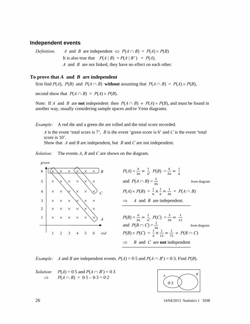
Independent events Definition. A and B are independent ⇔ P(A ∩ B) = P(A) × P(B) It is also true that P(A | B) = P(A | B′ ) = P(A). A and B are not linked, they have no effect on each other.

To prove that A and B are independent first find P(A), P(B) and P(A ∩ B) without assuming that P(A ∩ B) = P(A) × P(B),

second show that P(A ∩ B) = P(A) × P(B).

Note: If A and B are not independent then P(A ∩ B) ≠ P(A) × P(B), and must be found in another way, usually considering sample spaces and/or Venn diagrams. Example: A red die and a green die are rolled and the total score recorded.

A is the event ‘total score is 7’, B is the event ‘green score is 6’ and C is the event ‘total score is 10’. Show that A and B are independent, but B and C are not independent.

Solution: The events A, B and C are shown on the diagram.

green

6 × × × × × × P(A) = , P(B) =

5 × × × × × × and P(A ∩ B) = from diagram

4 × × × × × × P(A) × P(B) = = P(A ∩ B)

3 × × × × × × ⇒ A and B are independent.

2 × × × × × ×

1 × × × × × × P(B) = , P(C) =

and P(B ∩ C) = from diagram

1 2 3 4 5 6 red P(B) × P(C) = ≠ P(B ∩ C)

⇒ B and C are not independent Example: A and B are independent events. P(A) = 0⋅5 and P(A ∩ B′) = 0⋅3. Find P(B).

Solution: P(A) = 0⋅5 and P(A ∩ B′) = 0⋅3

⇒ P(A ∩ B) = 0⋅5 – 0⋅3 = 0⋅2

A

C

B

0⋅3

A B


But P(A ∩ B) = P(A) × P(B) ⇒ 0⋅2 = 0⋅5 × P(B)

⇒ P(B) = ··

= 0⋅4

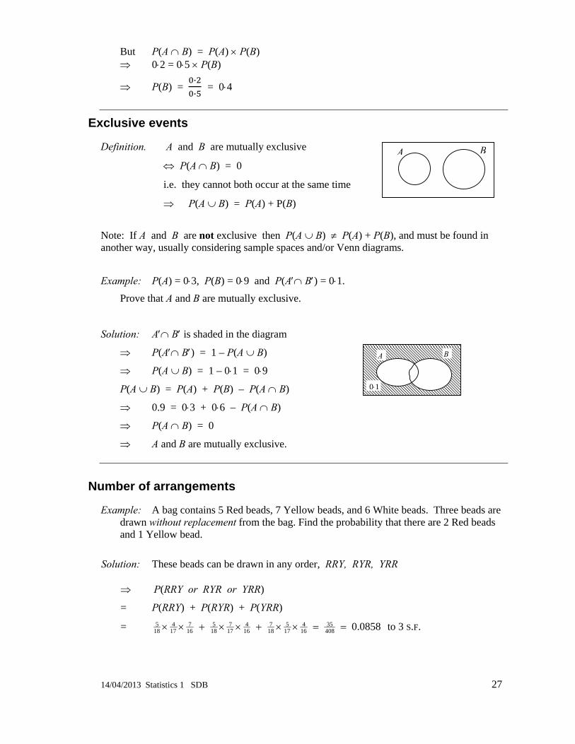
Exclusive events

Definition. A and B are mutually exclusive

⇔ P(A ∩ B) = 0

i.e. they cannot both occur at the same time

⇒ P(A ∪ B) = P(A) + P(B)

Note: If A and B are not exclusive then P(A ∪ B) ≠ P(A) + P(B), and must be found in another way, usually considering sample spaces and/or Venn diagrams.

Example: P(A) = 0⋅3, P(B) = 0⋅9 and P(A′∩ B′) = 0⋅1.

Prove that A and B are mutually exclusive.

Solution: A′∩ B′ is shaded in the diagram

⇒ P(A′∩ B′) = 1 – P(A ∪ B)

⇒ P(A ∪ B) = 1 – 0⋅1 = 0⋅9

P(A ∪ B) = P(A) + P(B) – P(A ∩ B)

⇒ 0.9 = 0⋅3 + 0⋅6 – P(A ∩ B)

⇒ P(A ∩ B) = 0

⇒ A and B are mutually exclusive.

Number of arrangements

Example: A bag contains 5 Red beads, 7 Yellow beads, and 6 White beads. Three beads are drawn without replacement from the bag. Find the probability that there are 2 Red beads and 1 Yellow bead.

Solution: These beads can be drawn in any order, RRY, RYR, YRR

⇒ P(RRY or RYR or YRR)

= P(RRY) + P(RYR) + P(YRR)

= 0858.040835

164

175

187

164

177

185

167

174

185 ==××+××+×× to 3 S.F.

A B

A B

0⋅1


You must always remember the possibility of more than one order. In rolling four DICE, exactly TWO SIXES can occur in six ways:

SSNN, SNSN, SNNS, NSSN, NSNS, NNSS, each of which would have the same

probability =

and so the probability of exactly two sixes with four dice is 6 × = .

7 Correlation Scatter diagrams

Positive, negative, no correlation & line of best fit.

no correlation positive correlation negative correlation

The pattern of a scatter diagram shows linear correlation in a general manner. A line of best fit can be draw by eye, but only when the points nearly lie on a straight line.

Product moment correlation coefficient, PMCC

Formulae The are all similar to each other and make other formulae simpler to learn and use:

Sxy = = Sxx = = Syy = =

The PMCC r = yyxx

xy

SS

S, –1 ≤ r ≤ +1 for proof, see appendix

To calculate the PMCC first calculate Sxx, Syy and Sxy using the second formula on each line. N.B. These formulae are all in the formula booklet.

1

1

1


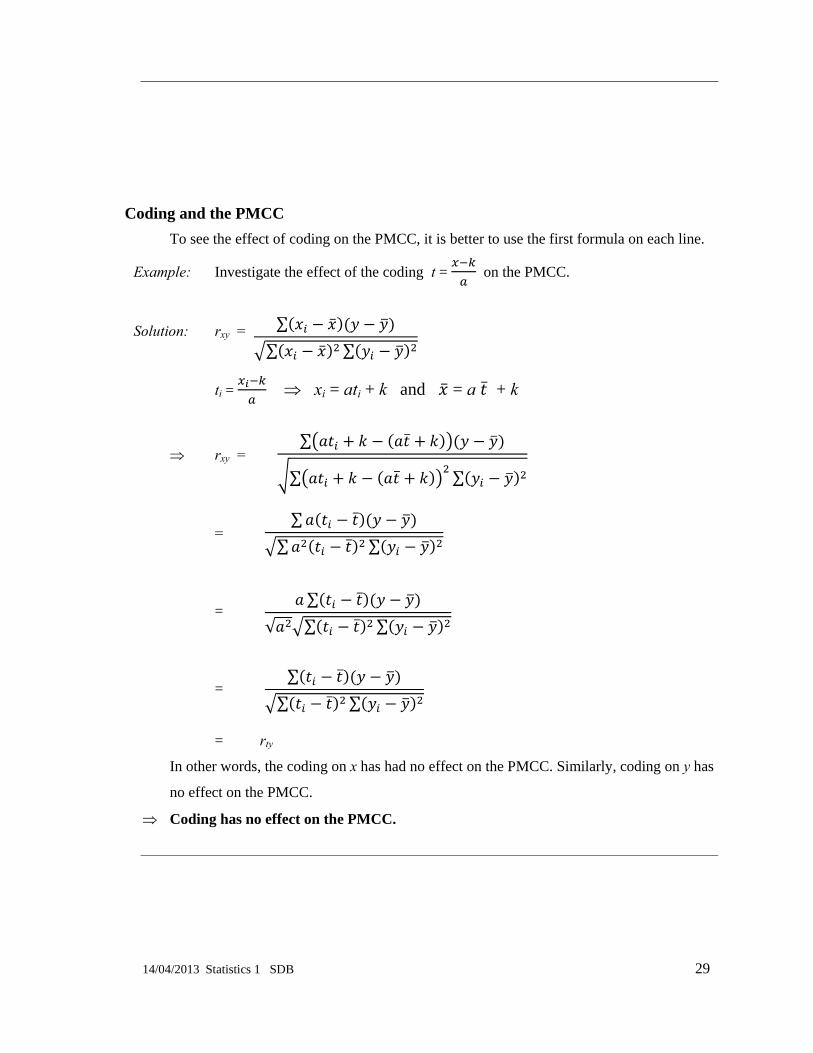
Coding and the PMCC To see the effect of coding on the PMCC, it is better to use the first formula on each line.

Example: Investigate the effect of the coding t = on the PMCC.

Solution: rxy =

ti = ⇒ xi = ati + k and = a + k

⇒ rxy =

=

=

=

= rty

In other words, the coding on x has had no effect on the PMCC. Similarly, coding on y has

no effect on the PMCC.

⇒ Coding has no effect on the PMCC.

∑∑ ∑

∑

∑ ∑

∑∑ ∑

∑

√ ∑ ∑

∑∑ ∑


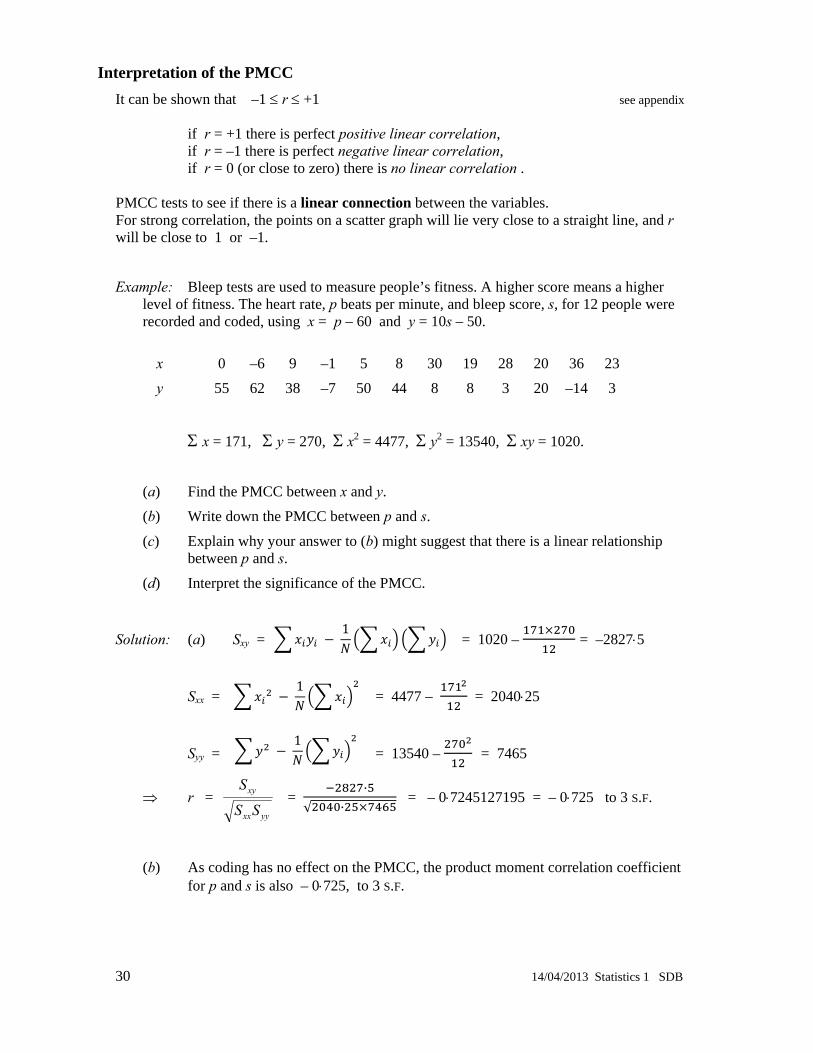
Interpretation of the PMCC It can be shown that –1 ≤ r ≤ +1 see appendix

if r = +1 there is perfect positive linear correlation, if r = –1 there is perfect negative linear correlation, if r = 0 (or close to zero) there is no linear correlation .

PMCC tests to see if there is a linear connection between the variables. For strong correlation, the points on a scatter graph will lie very close to a straight line, and r will be close to 1 or –1.

Example: Bleep tests are used to measure people’s fitness. A higher score means a higher level of fitness. The heart rate, p beats per minute, and bleep score, s, for 12 people were recorded and coded, using x = p – 60 and y = 10s – 50.

x 0 –6 9 –1 5 8 30 19 28 20 36 23

y 55 62 38 –7 50 44 8 8 3 20 –14 3

Σ x = 171, Σ y = 270, Σ x2 = 4477, Σ y2 = 13540, Σ xy = 1020.

(a) Find the PMCC between x and y.

(b) Write down the PMCC between p and s.

(c) Explain why your answer to (b) might suggest that there is a linear relationship between p and s.

(d) Interpret the significance of the PMCC.

Solution: (a) Sxy = = 1020 – = –2827⋅5

Sxx = = 4477 – = 2040⋅25

Syy = = 13540 – = 7465

⇒ r = yyxx

xy

SS

S =

·√ ·

= – 0⋅7245127195 = – 0⋅725 to 3 S.F.

(b) As coding has no effect on the PMCC, the product moment correlation coefficient for p and s is also – 0⋅725, to 3 S.F.

1

1

1


(c) r = – 0⋅725 is ‘quite close’ to –1, and therefore the points on a scatter diagram would lie close to a straight line

⇒ there is evidence of a linear relation between p and s.

(d) There is negative correlation between p and s, which means that as heart rate increases, the bleep score decreases, or people with higher heart rate tend to have lower bleep scores.

8 Regression Explanatory and response variables

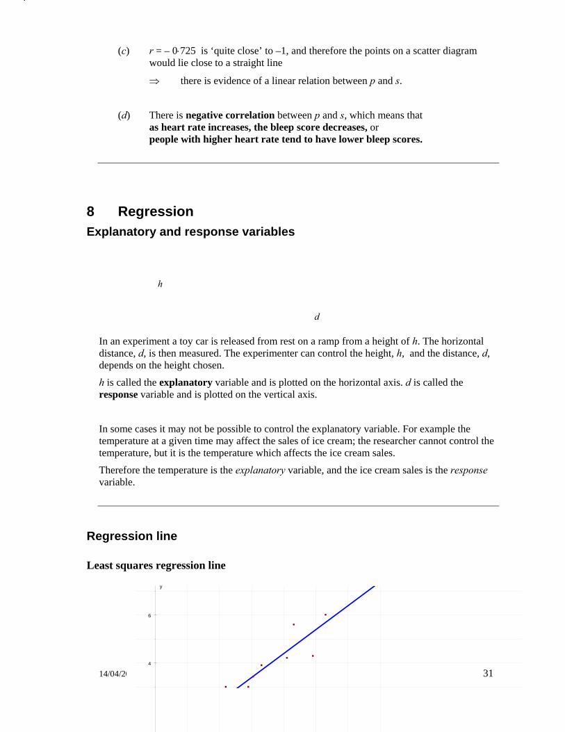
In an experiment a toy car is released from rest on a ramp from a height of h. The horizontal distance, d, is then measured. The experimenter can control the height, h, and the distance, d, depends on the height chosen.

h is called the explanatory variable and is plotted on the horizontal axis. d is called the response variable and is plotted on the vertical axis.

In some cases it may not be possible to control the explanatory variable. For example the temperature at a given time may affect the sales of ice cream; the researcher cannot control the temperature, but it is the temperature which affects the ice cream sales.

Therefore the temperature is the explanatory variable, and the ice cream sales is the response variable.

Regression line

Least squares regression line

h

d

,4

6

y


The scatter diagram shows the regression line of y on x. The regression line is drawn to minimise the sum of the squares of the vertical distances between the line and the points.

It can be shown that the regression line has equation y = a + bx, where b = xx

xy

SS

,

also that the regression line passes through the ‘mean point’, ( , ),

and so we can find a from the equation = a + b ⇒ a = – b

Interpretation In the equation y = a + bx

a is the value of y when x is zero (or when x is not present) b is the amount by which y increases for an increase of 1 in x.

You must write your interpretation in the context of the question.

Example: A local authority is investigating the cost of reconditioning its incinerators. Data from 10 randomly chosen incinerators were collected. The variables monitored were the operating time x (in thousands of hours) since last reconditioning and the reconditioning cost y (in £1000). None of the incinerators had been used for more than 3000 hours since last reconditioning.

The data are summarised below,

Σx = 25.0, Σx2 = 65.68, Σy = 50.0, Σy2 = 260.48, Σxy = 130.64.

(a) Find the equation of the regression line of y on x.

(b) Give interpretations of a and b.

Solution:

(a) = · = 2⋅50, =

· = 5⋅00,

Sxy = 130⋅64 – · · = 5⋅64, Sxx = 65.68 –

· = 3⋅18


⇒ b = = ..

= 1⋅773584906

⇒ a = – b = 5⋅00 – 1⋅773584906 × 2⋅50 = 0⋅5660377358

⇒ regression line equation is y = 0⋅566 + 1⋅77x to 3 S.F.

(b) a is the cost in £1000 of reconditioning an incinerator which has not been used, so the cost of reconditioning an incinerator which has not been used is £566. (a is the value of y when x is zero)

b is the increase in cost (in £1000) of reconditioning for every extra 1000 hours of use, so it costs an extra £1774 to recondition an incinerator for every 1000 hours of use. (b is the gradient of the line)

9 Discrete Random Variables Random Variables

A random variable must take a numerical value: Examples: the number on a single throw of a die the height of a person the number of cars travelling past a fixed point in a certain time But not the colour of hair as this is not a number

Continuous and discrete random variables

Continuous random variables A continuous random variable is one which can take any value in a certain interval; Examples: height, time, weight.

Discrete random variables

A discrete random variable can only take certain values in an interval Examples: Score on die (1, 2, 3, 4, 5, 6) Number of coins in pocket (0, 1, 2, ...)

Probability distributions

A probability distribution is the set of possible outcomes together with their probabilities,

similar to a frequency distribution or frequency table.


Example:

score on two dice, X 2 3 4 5 6 7 8 9 10 11 12

probability, f (x)

is the probability distribution for the random variable, X, the total score on two dice.

Note that the sum of the probabilities must be 1, i.e. 1)(12

2==∑

=xxXP .

Cumulative probability distribution

Just like cumulative frequencies, the cumulative probability, F, that the total score on two dice is less than or equal to 4 is F(4) = P(X ≤ 4) = .

Note that F(4.3) means P(X ≤ 4.3) and seeing as there are no scores between 4 and 4.3 this is the same as P(X ≤ 4) = F(4).

Expectation or expected values

Expected mean or expected value of X. For a discrete probability distribution the expected mean of X , or the expected value of X is

μ = E[X] =

Expected value of a function The expected value of any function, f (X), is defined as E[X] =

Note that for any constant, k, E[k] = k, since ∑ = k ∑ = k × 1 = k

Expected variance The expected variance of X is

Var , or σ 2 = Var[X] = E[(X – μ)2] = E[X 2] – μ 2 = E[X 2] – (E[X])2


Expectation algebra E[aX + b] =

= aE[X] + b since ∑ = μ, and ∑ 1

Var[aX + b] = E[(aX + b)2] – (E[(aX + b)])2

= E[(a2X 2 + 2abX + b2)]) – (aE[X] + b)2

= {a2 E[X 2] + 2ab E[X] + E[b2]} – {a2 (E[X])2 + 2ab E[X] + b2} = a2 E[X 2] – a2 (E[X])2 = a2{E[X 2] – (E[X])2} = a2 Var[X]

Thus we have two important results:

E[aX + b] = aE[X] + b

Var[aX + b] = a2 Var[X]

which are equivalent to the results for coding done earlier.

Example: A fair die is rolled and the score recorded.

(a) Find the expected mean and variance for the score, X.

(b) A ‘prize’ is awarded which depends on the score on the die. The value of the prize

is $Z = 3X – 6. Find the expected mean and variance of Z.

Solution: (a) score probability xi pi xi2pi

1

2

3

4

5

6

⇒ μ = E[X] = ∑ = = 3

and σ 2 = E[X 2] – (E[X])2 = – = = 2


⇒ The expected mean and variance for the score, X, are μ = 3 and σ 2 = 2

(b) Z = 3X – 6

⇒ E[Z] = E[3X – 6] = 3E[X] – 6 = 10 – 6 = 4

and Var[Z] = Var[3X – 6] = 32 Var[X] = 9 × = 26

⇒ The expected mean and variance for the prize, $Z, are μ = 4 and σ 2 = 26

The discrete uniform distribution

Conditions for a discrete uniform distribution • The discrete random variable X is defined over a set of n distinct values

• Each value is equally likely, with probability 1/n .

Example: The random variable X is defined as the score on a single die. X is a discrete

uniform distribution on the set {1, 2, 3, 4, 5, 6}

The probability distribution is

Score 1 2 3 4 5 6

Probability

Expected mean and variance For a discrete uniform random variable, X defined on the set {1, 2, 3, 4, ..., n},

X 1 2 3 4 ... ... n Probability

By symmetry we can see that the Expected mean = μ = E[X] = (n + 1),

or μ = E[X] = ∑ = 1 × + 2 × + 3 × + … + n ×

= (1 + 2 + 3 + … + n) × = n(n + 1) × = (n + 1)


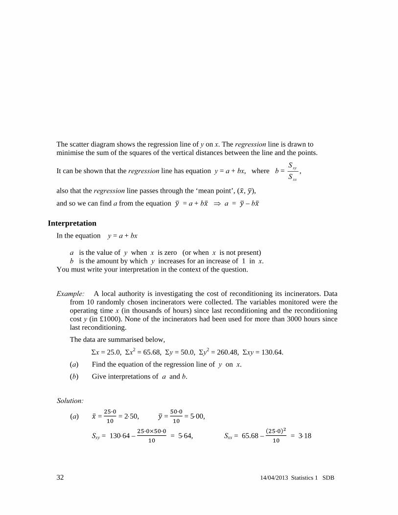
The expected variance,

Var[X] = σ 2 = E[X 2] – (E[X])2 = ∑

= (12 + 22 + 32 + … + n2) × − 1

= n(n + 1)(2n + 1) × − (n + 1) 2 since Σ i2 = n(n + 1)(2n + 1)

= (n + 1){(8n + 4) − (6n + 6)}

= (n + 1) (2n − 2)

⇒ Var[X] = σ 2 = (n2 − 1)

These formulae can be quoted in an exam (if you learn them!).

Non-standard uniform distribution The formulae can sometimes be used for non-standard uniform distributions. Example: X is the score on a fair 10 sided spinner. Define Y = 5X + 3.

Find the mean and variance of Y.

Y is the distribution {8, 13, 18, … 53}, all with the same probability .

Solution: X is a discrete uniform distribution on the set {1, 2, 3, …, 10}

⇒ E[X] = (n + 1) = 5

and Var[X] = (n2 − 1) = = 8

⇒ E[Y] = E[5X + 3] = 5E[X] + 3 = 30

and Var[X] = Var[5X + 3] = 52 Var[X] = 25 × = 206

⇒ mean and variance of Y are 27 and 206 .


10 The Normal Distribution N(μ, σ2)

The standard normal distribution N(0, 12)

To find other probabilities, sketch the curve and use your head

The diagram shows the standard normal distribution

Mean, μ, = 0

Standard deviation, σ, = 1

The tables give the area, Φ(z), from –∞ upto z;

Example: P(Z < –1⋅23)

= area upto –1⋅23 = Φ(–1⋅23)

= area beyond +1⋅23 = 1 – Φ(+1⋅23)

= 1 – 0⋅8907 = 0⋅1093 to 4 D.P. −1⋅23 1⋅23

z

-3 -2 -1 1 2 3z

-3 -2 -1 1 2 3z


The general normal distribution N(μ, σ2)

Use of tables

Example: The length of life (in months) of Blowdri’s hair driers is approximately Normally distributed with mean 90 months and standard deviation 15 months.

(a) Each drier is sold with a 5 year guarantee. What proportion of driers fail before the guarantee expires?

(b) The manufacturer decides to change the length of the guarantee so that no more than 1% of driers fail during the guarantee period. How long should he make the guarantee?

Solution:

(a) X is the length of life of drier ⇒ X ~ N(90, 152).

5 years = 60 months

⇒ we want P(X < 60) = area upto 60

⇒ Z = 0.215

9060−=

−=

−σμX

so we want area to left of Z = –2

= Φ(–2) = 1 – Φ(2)

= 1 – 0⋅9772 = 0⋅0228 to 4 D.P. from tables.

⇒ the proportion of hair driers failing during the guarantee period is 0.0288 to 4 D.P. (b) Let the length of the guarantee be t years

⇒ we need P(X < t) = 0⋅01.

To use the tables for a Normal distribution with

mean μ and standard deviation σ

We use Z σμ−

=X (see appendix) and look

in the tables under this value of Z μ-2σ μ -σ μ μ+σ μ+2σ

Z

60 90

t 90

0⋅01

-3 -2 -1 1 2 3z

x

x


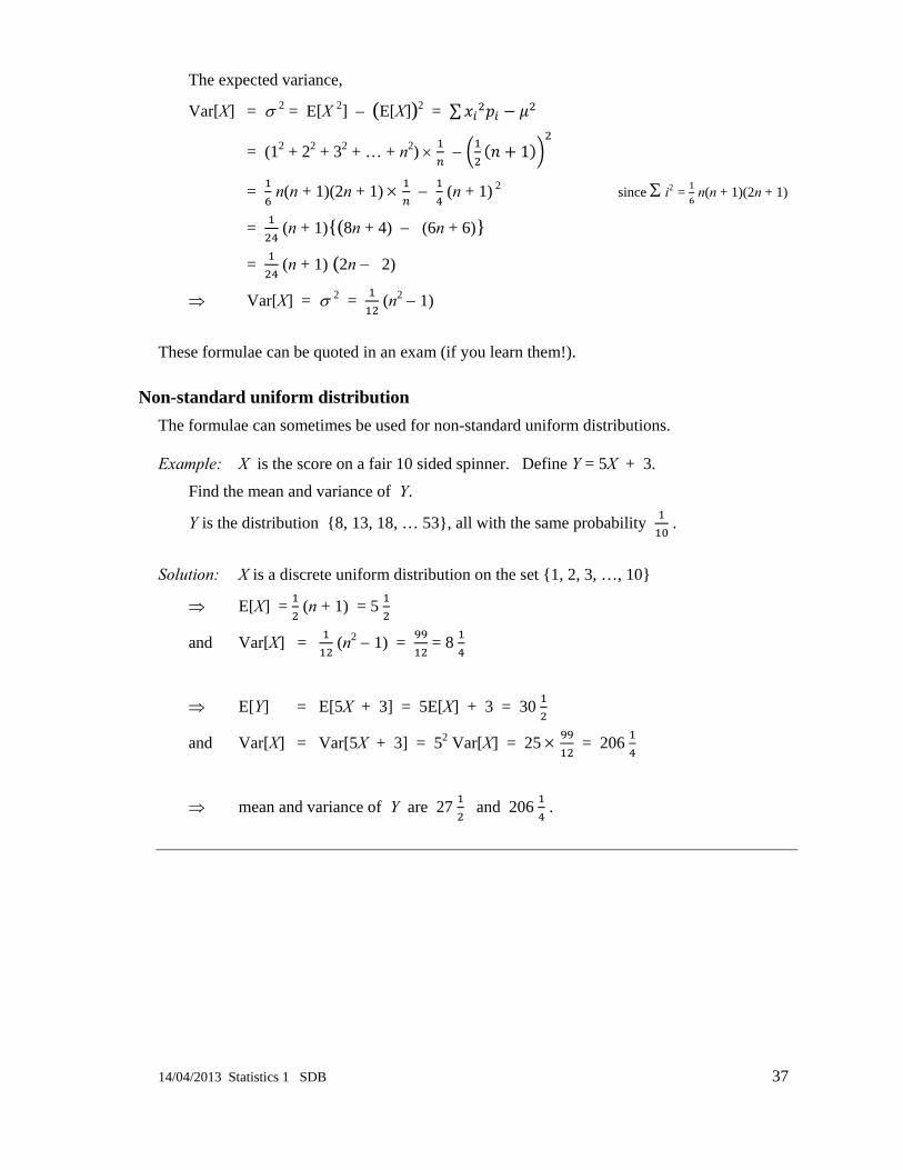
We need the value of Z such that Φ(Z) = 0⋅01

From the tables Z = –2⋅3263 to 4 D.P. from tables (remember to look in the small table

after the Normal tables)

Standardising the variable

⇒ Z = 15

90−=

− tXσμ

⇒ 3263215

90⋅−=

−t to 4 D.P. from tables

⇒ t = 55⋅1 to 3 S.F.

so the manufacturer should give a guarantee period of 55 months (4 years 7 months)

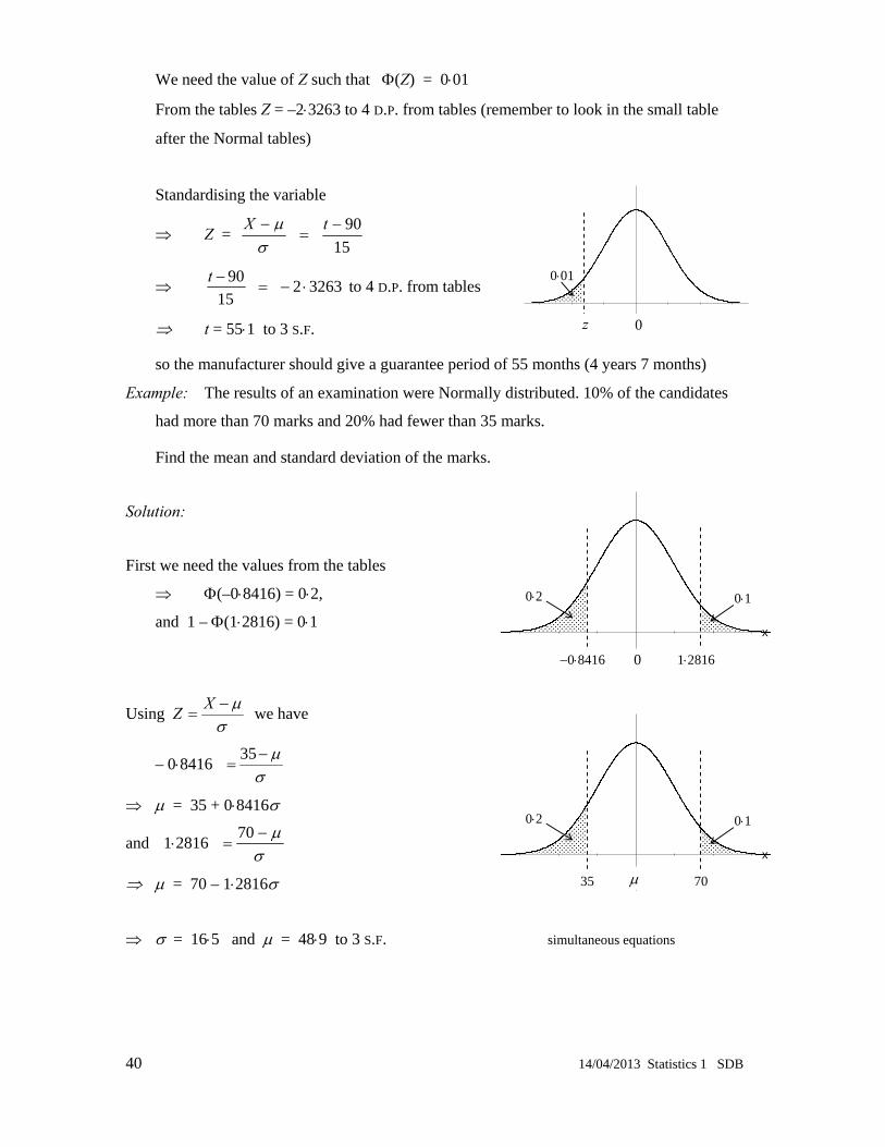
Example: The results of an examination were Normally distributed. 10% of the candidates

had more than 70 marks and 20% had fewer than 35 marks.

Find the mean and standard deviation of the marks.

Solution:

First we need the values from the tables

⇒ Φ(–0⋅8416) = 0⋅2,

and 1 – Φ(1⋅2816) = 0⋅1

Using Z σμ−

=X we have

– 0⋅8416 σμ−

=35

⇒ μ = 35 + 0⋅8416σ

and 1⋅2816 σ

μ−=

70

⇒ μ = 70 – 1⋅2816σ

⇒ σ = 16⋅5 and μ = 48⋅9 to 3 S.F. simultaneous equations

x

0

0⋅2 0⋅1

−0⋅8416 1⋅2816

x

μ

0⋅2 0⋅1

35 70

z 0

0⋅01


Example: The weights of chocolate bars are normally distributed with mean 205 g and

standard deviation 2⋅6 g. The stated weight of each bar is 200 g.

(a) Find the probability that a single bar is underweight.

(b) Four bars are chosen at random. Find the probability that fewer than two bars are underweight.

Solution:

(a) Let W be the weight of a chocolate bar, W ~ N(205, 2⋅62).

Z = = ·

= – 1⋅9230769…

P(W < 200) = P(Z < – 1⋅92) = 1 – Φ(1⋅92) = 1 – 0⋅9726

⇒ probability of an underweight bar is 0⋅0274.

(b) We want the probability that 0 or 1 bars chosen from 4 are underweight.

Let U be underweight and C be correct weight.

P(1 underweight) = P(CCCU) + P(CCUC) + P(CUCC) + P(UCCC)

= 4 × 0⋅0274 × 0⋅97263 = 0⋅1008354753

P(0 underweight) = 0⋅92764 = 0⋅7403600224

⇒ the probability that fewer than two bars are underweight = 0⋅841 to 3 S.F.


11 Context questions and answers

Accuracy

You are required to give your answers to an appropriate degree of accuracy.

There is no hard and fast rule for this, but the following guidelines should never let you down.

1. If stated in the question give the required degree of accuracy. 2. When using a calculator, give 3 S.F.

unless finding Sxx,, Sxy etc. in which case you can give more figures – you should use all figures when finding the PMCC or the regression line coefficients.

3. Sometimes it is appropriate to give a mean to 1 or 2 D.P. rather than 3 S.F. 4. When using the tables and doing simple calculations (which do not need a calculator),

you should give 4 D.P.

Statistical models

Question 1

(a) Explain briefly what you understand by

(i) a statistical experiment,

(ii) an event.

(b) State one advantage and one disadvantage of a statistical model.

Answer (a) a test/investigation/process for collecting data to provide evidence to test a

hypothesis.

A subset of possible outcomes of an experiment

(b) Quick, cheap can vary the parameters and predict

Does not replicate real world situation in every detail.


Question 2

Statistical models can be used to describe real world problems. Explain the process involved in the formulation of a statistical model.

Answer Observe real world problem

Devise a statistical model and collect data

Compare observed against expected outcomes and test the model

Refine model if necessary

Question 3

(a) Write down two reasons for using statistical models.

(b) Give an example of a random variable that could be modelled by

(i) a normal distribution,

(ii) a discrete uniform distribution.

Answer

(a) To simplify a real world problem

To improve understanding / describe / analyse a real world problem

Quicker and cheaper than using real thing

To predict possible future outcomes

Refine model / change parameters possible Any 2

(b) (i) height, weight, etc. (ii) score on a face after rolling a fair die

Histograms

Question 1

Give a reason to justify the use of a histogram to represent these data.

Answer

The variable (minutes delayed) is continuous.

Averages

Question 1

Write down which of these averages, mean or median, you would recommend the company to use. Give a reason for your answer.

Answer


The median, because the data is skewed.

Question 2

State whether the newsagent should use the median and the inter-quartile range or the mean and the standard deviation to compare daily sales. Give a reason for your answer.

Answer

Median & IQR as the data is likely to be skewed

Question 3

Compare and contrast the attendance of these 2 groups of students.

Answer

Median 2nd group < Median 1st group;

Mode 1st group > Mode 2nd group;

2nd group had larger spread/IQR than 1st group

Only 1 student attends all classes in 2nd group

Question 4

Compare and contrast these two box plots.

Answer

Median of Northcliffe is greater than median of Seaview.

Upper quartiles are the same

IQR of Northcliffe is less than IQR of Seaview

Northcliffe positive skew, Seaview negative skew

Northcliffe symmetrical, Seaview positive skew (quartiles) Range of Seaview greater than range of Northcliffe

any 3 acceptable comments

Skewness

Question 1

Comment on the skewness of the distribution of bags of crisps sold per day. Justify your answer.

Answer

Q2 − Q1 = 7; Q3 − Q2 = 11; Q3 − Q2 > Q2 − Q1 so positive skew.


Question 2

Give two other reasons why these data are negatively skewed.

Answer

For negative skew; Mean < median < mode: 49⋅4 < 52 < 56

Q3 – Q2 < Q2 – Q1: 8 < 17

Question 3

Describe the skewness of the distribution. Give a reason for your answer.

Answer No skew or slight negative skew.

0.22 = Q3 − Q2 ≈ Q2 − Q1 = 0.23 or 0.22 = Q3 − Q2 < Q2 − Q1 = 0.23

or mean (3.23) ≈ median (3.25), or mean (3.23) < median (3.25)

Correlation

Question 1

Give an interpretation of your PMCC (–0⋅976)

Answer As height increases, temperature decreases (must be in context).

Question 2

Give an interpretation of this value, PMCC = –0⋅862.

Answer As sales at one petrol station increases, sales at the other decrease (must be in context).

Question 3

Give an interpretation of your correlation coefficient, 0⋅874.

Answer Taller people tend to be more confident (must be in context).


Question 4

Comment on the assumption that height and weight are independent.

Answer

Evidence (in question) suggests height and weight are positively correlated / linked, therefore the assumption of independence is not sensible (must be in context).

Regression

Question 1

Suggest why the authority might be cautious about making a prediction of the reconditioning cost of an incinerator which had been operating for 4500 hours since its last reconditioning.

Answer 4500 is well outside the range of observed values, and there is no evidence that the model will apply.

Question 2

Give an interpretation of the slope, 0⋅9368, and the intercept, 19, of your regression line.

Answer

The slope, b – for every extra hour of practice on average 0⋅9368 fewer errors will be made

The intercept, a – without practice 19 errors will be made.

Question 3

Interpret the value of b (coefficient of x in regression line).

Answer

3 extra ice-creams are sold for every 1°C increase in temperature

Question 4

At 1 p.m. on a particular day, the highest temperature for 50 years was recorded. Give a reason why you should not use the regression equation to predict ice cream sales on that day.

Answer Temperature is likely to be outside range of observed values.


Question 5

Interpret the value of a, (regression line)

Answer Number of ……… sold if no money spent on advertising

Question 6

Give a reason to support fitting a regression model of the form y = a + bx to these data.

Answer

Points on the scatter graph lie close to a straight line.

Question 7

Give an interpretation of the value of b.

Answer

A flight costs £2.03 (or about £2) for every extra 100km or about 2p per extra km.

Discrete uniform distribution

Question 1

A discrete random variable is such that each of its values is assumed to be equally likely.

(a) Write down the name of the distribution that could be used to model this random variable.

(b) Give an example of such a distribution.

(c) Comment on the assumption that each value is equally likely.

(d) Suggest how you might refine the model in part (a).

Answer (a) Discrete uniform

(b) Example – Tossing a fair die /coin, drawing a card from a pack

(c) Useful in theory – allows problems to be modelled, but the assumption might not be true in practice

(d) Carry out an experiment to find the probabilities – which might not fit the model.

Normal distribution

Question 1

The random variable X is normally distributed with mean 177⋅0 and standard deviation 6⋅4.

It is suggested that X might be a suitable random variable to model the height, in cm, of adult males.


(a) Give two reasons why this is a sensible suggestion.

(b) Explain briefly why mathematical models can help to improve our understanding of real-world problems.

Answer (a) Male heights cluster round a central height of approx 177/178 cm

Height is a continuous random variable.

Most male heights lie within 177 ± 3× 6.4

(b) Simplifies real world problems

Enable us to gain some understanding of real world problems more quickly/cheaply.

Question 2

Explain why the normal distribution may not be suitable to model the number of minutes that motorists are delayed by these roadworks.

Answer For this data skewness is 3.9, whereas a normal distribution is symmetrical and has no skew.

Question 3

Describe two features of the Normal distribution

Answer Bell shaped curve; symmetrical about the mean; 95% of data lies within 2 s.d. of mean; etc. (any 2).

Question 4

Give a reason to support the use of a normal distribution in this case.

Answer Since mean and median are similar (or equal or very close), the distribution is (nearly)

symmetrical and a normal distribution may be suitable.

Allow mean or median close to mode/modal class ⇒ ), the distribution is (nearly) symmetrical and a normal distribution may be suitable.


12 Appendix

–1 ≤ P.M.C.C. ≤ 1

Cauchy-Schwartz inequality Consider (a1

2 + a22)(b1

2 + b22) – (a1b1 + a2b2)2

= a12 b1

2 + a12 b2

2 + a22 b1

2 + a22 b2

2 – a12 b1

2 – 2a1b1a2b2 – a22 b2

2

= a12 b2

2 – 2a1b1a2b2+ a22 b1

2

= (a1b2 – a2b1)2 ≥ 0

⇒ (a12 + a2

2)(b12 + b2

2) – (a1b1 + a2b2)2 ≥ 0

⇒ (a1b1 + a2b2)2 ≤ (a12 + a2

2)(b12 + b2

2)

This proof can be generalised to show that

(a1b1 + a2b2 + … + anbn)2 ≤ (a12 + a2

2 + … + an2)(b1

2 + b22 + … + bn

2)

or

P.M.C.C. between –1 and +1 In the above proof, take ai = (xi – ), and bi = (yi – )

⇒ Sxy = Σ (xi – )(yi – ) = Σ aibi

Sxx = Σ (xi – )2 = Σ ai2 and Syy = Σ (yi – )2 = Σ bi

2

P.M.C.C. = r =

⇒ r 2 = = ∑

∑ ∑ ≤ 1 using the Cauchy-Schwartz inequality


⇒ –1 ≤ r ≤ +1

Regression line and coding

The regression line of y on x has equation y = a + bx, where b = , and a = – b .

Using the coding x = hX + m, y = gY + n, the regression line for Y on X is found by writing

gY + n instead of y, and hX + m instead of x in the equation of the regression line of y on x,

⇒ gY + n = a + b(hX + m)

⇔ Y = + bX … … … … … equation I.

Proof = h + m, and = g + n

⇒ (x – ) = (hX + m) – (h + m) = (hX – h ), and similarly (y – ) = (gY – g ).

Let the regression line of y on x be y = a + bx, and

let the regression line of Y on X be Y = α + β X.

Then b = and a = – b

also β = and α = – β .

b = = ∑∑ ∑

∑ ∑∑ ∑

∑

⇒ b = β

⇒ β =

α = – β = = since a = – b

and so

Y = α + β X ⇔ Y = + bX

which is the same as equation I.


Normal Distribution, Z =

The standard normal distribution with mean 0 and standard deviation 1 has equation

√

The normal distribution tables allow us to find the area between Z1 and Z2.

1

√2

The normal distribution with mean μ and standard deviation σ has equation

√

1√2

Using the substitution z =

dz = dx, Z1 = and Z2 =

1

√2

= the area under the standard normal curve, which we can find from the tables using

Z1 = and Z2 = . Thus Φ Φ

x

μ X1 X2

f (x)

x

0 Z1 Z2

φ (z)

z


Index

accuracy, 41 box plots, 16 class boundaries, 7 correlation, 27

context questions, 44

cumulative frequency, 6 cumulative frequency curves, 8

cumulative probability distribution, 33 discrete uniform distribution, 35

context questions, 46 expected mean, 35 expected variance, 35

exclusive events, 26 expectation. See expected values expectation algebra, 33 expected values, 33

expected mean, 33 expected variance, 33

frequency distributions, 6 grouped frequency distributions, 7

histograms, 8 context questions, 42

independent events, 25 interquartile range, 13, 19 mean, 10

coding, 11 when to use, 12

median discrete lists and tables, 13 grouped frequency tables, 14 when to use, 12

mode, 10 when to use, 12

normal distribution, 37 context questions, 46 general normal distribution, 37 standard normal distribution, 37 standardising the variable, proof, 50

outliers, 16 percentiles, 16 probability

diagrams for two dice etc, 23 number of arrangements, 26 rules, 22 Venn diagrams, 22

probability distributions, 32 product moment correlation coefficient, 27

between -1 and +1, 48 coding, 28 interpretation, 28

quartiles discrete lists and tables, 13 grouped frequency tables, 14

random variables, 32 continuous, 32 discrete, 32

range, 19 regression, 30

context questions, 45 explanatory variable, 30 response variable, 30

regression line, 30 interpretation, 31

regression line and coding proof, 49

relative frequency, 22 sample spaces, 22 scatter diagrams, 27

line of best fit, 27

skewness, 17 context questions, 43

standard deviation, 19 statistical modelling, 5 statistical models

context questions, 41

stem and leaf diagrams, 7 tree diagrams, 24 variables

continuous variables, 6 discrete variables, 6 qualitative variables, 6 quantitative variables, 6

variance, 19 coding, 20

statistics 1 revision notes - wordpress.com · statistics 1 revision notes ... e.g. railway...

Documents