A&A 552, A138 (2013)DOI: 10.1051/0004-6361/201220456c© ESO 2013

Astronomy&

Astrophysics

Statistical seismology of transverse waves in the solar corona

E. Verwichte1,2, T. Van Doorsselaere2, R. S. White1, and P. Antolin2

1 Department of Physics, University of Warwick, Coventry CV4 7AL, UKe-mail: Erwin.Verwichte@warwick.ac.uk

2 Centre for Plasma Astrophysics, Department of Mathematics, Katholieke Universiteit Leuven, Celestijnenlaan 200B, 3001 Leuven,Belgium

Received 27 September 2012 / Accepted 27 February 2013

ABSTRACT

Context. Observations show that transverse oscillations commonly occur in solar coronal loops. The rapid damping of these waveshas been attributed to resonant absorption. The oscillation characteristics carries information of the structuring of the corona. However,self-consistent seismological methods that extract information from individual oscillations are limited because there are fewer observ-ables than unknown parameters in the model, and the problem is underdetermined. Furthermore, it has been shown that one-to-onecomparisons of the observed scaling of period and damping times with wave damping theories are misleading.Aims. We aim to investigate whether seismological information can be gained from the observed scaling laws in a statistical sense.Methods. A statistical approach is used whereby scaling laws are produced by forward modelling using distributions of values forkey loop cross-sectional structuring parameters. We study two types of observations: 1) transverse loops oscillations as seen mainlywith TRACE and SDO and 2) running transverse waves seen with the Coronal Multichannel Polarimeter (CoMP).Results. We demonstrate that the observed period-damping time scaling law does provide information about the physical dampingmechanism, if observations are collected from as wide range of periods as possible and a comparison with theory is performed in astatistical sense. The distribution of the ratio of damping time over period, i.e. the quality factor, has been derived analytically andfitted to the observations. A minimum value for the quality factor of 0.65 has been found. From this, a constraint linking the rangesof possible values for the density contrast and inhomogeneity layer thickness is obtained for transverse loop oscillations. If the layerthickness is not constrained, then the density contrast is at most equal to 3. For transverse waves seen by CoMP, it is found that theratio of maximum to minimum values for these two parameters has to be less than 2.06; i.e., the sampled values for the layer thicknessand Alfvén travel time come from a relatively narrow distribution.Conclusions. Now that more and more transverse loop oscillations have been analysed, a statistical approach to coronal seismologybecomes possible. Using the observed data cloud, we have found restrictions to the loop’s density contrast and inhomogeneity layerthickness. Surprisingly, for running waves, narrow distributions for loop parameters have been found.

Key words. Sun: oscillations – magnetohydrodynamics (MHD)

1. Introduction

Transverse waves are pervasive in the solar corona. They havebeen detected with confidence ever since 1998 (Aschwandenet al. 1999; Nakariakov et al. 1999) in the form of transverseloop oscillations (TLOs). To date, more than 50 TLOs havebeen reported with periods ranging between 100 s and 3 h(Aschwanden et al. 2002; Wang & Solanki 2004; Verwichte et al.2004; Hori et al. 2005, 2007; Van Doorsselaere et al. 2007, 2009;De Moortel & Brady 2007; Verwichte et al. 2009, 2010; Mrozek2011; White & Verwichte 2012; White et al. 2012; Verwichteet al. 2012). The majority of these oscillations have been stud-ied using EUV imagers, such as TRACE (Handy et al. 1999),EUVI/STEREO (Howard et al. 2008) and AIA/SDO (Lemenet al. 2012). They are reported to dampen quickly with oscil-lation quality factors in the range 0.6–5.4.

Tomczyk et al. (2007) used ground-based spectral mea-surements with the Coronal Multichannel Polarimeter (CoMP)(Tomczyk et al. 2008) to demonstrate that small-amplitude prop-agating transverse waves are ubiquitous in the solar corona. Thisresult seems to be supported by the recent report of runningtransverse waves in coronal loops by AIA/SDO (McIntosh et al.2011; Wang et al. 2012).

A widely accepted explanation for the rapid damping is themechanism of resonant absorption where the transverse wave

is considered to be an Alfvénic kink mode (or surface Alfvénmode Wentzel 1979; Goossens et al. 2012) whose nature evolvesthrough a resonance at a loop layer where its frequency matchesthe local Alfvén frequency, from a global transverse loop motionto a local, mainly azimuthal motion (Ruderman & Roberts 2002;Goossens et al. 2002). Once local, the mode cannot be observeddirectly and it then proceeds to dampen dissipatively, enhancedby phase-mixing (or alternatively collisionlessly). It is the rateof mode evolution from global to local that is observed as therapid damping of the transverse wave. The observed dampingtime depends on the structure of the Alfvén frequency across theloop.

Besides the loop’s average Alfvén speed and magnetic fieldstrength (Nakariakov & Ofman 2001), there is the potential forseismologically determining the loop cross-section profile, in-cluding the density contrast, which is difficult to measure di-rectly (e.g. Aschwanden et al. 2003; Schmelz et al. 2003; Terzo& Reale 2010). By combining the theories for the propagationand damping of the transverse wave it is possible to constrainthe unknown parameters in the problem (Verwichte et al. 2006)self-consistently. However, for the resonant absorption dampingmodel, the problem is under-determined and it is not possible todeduce both density contrast and the thickness of the inhomo-geneity layer independently (Arregui et al. 2007; Goossens et al.2008; Arregui & Asensio Ramos 2011).

Article published by EDP Sciences A138, page 1 of 9

A&A 552, A138 (2013)

Ofman & Aschwanden (2002) modelled the scaling rela-tions, e.g. between damping time and period, for different damp-ing mechanisms. They find that the observed scaling relationswere more compatible with phase mixing. However, it is pointedout by Arregui et al. (2008) that a one-to-one comparison be-tween the observed scaling and the linear scaling from resonantabsorption inherently makes the unrealistic assumption that allloops have the same cross-sectional structuring. In fact, by al-lowing the cross-sectional profile to vary between events, theyshow that the scaling from resonant absorption can easily de-part from linear. Thus, they conclude that scaling laws were notsufficient to distinguish damping mechanisms, because resonantabsorption can reproduce several dependencies using carefullychosen distributions of equilibrium parameters. However, nowit becomes possible to use the inverse approach. Since 2002(Aschwanden et al. 2002), the number of observations and therange of observed periods has increased. Given the observedscaling laws of periods and damping time, can we find infor-mation on the statistical distributions of equilibrium parametersof coronal loops that exist in the solar corona? In this article weshow that it is possible to use statistical and forward-modellingapproaches to model scaling laws of loops. This statistical, seis-mological information on the coronal loop ensemble can poten-tially help distinguish between different coronal loop models andheating mechanisms.

The paper is structured in two main parts. Section 2 statis-tically investigates the scaling of TLOs using two approaches.Section 3 studies the transverse waves seen by CoMP (Tomczyket al. 2007) statistically. We discuss our findings in Sect. 4.

2. Statistics of transverse loop oscillations

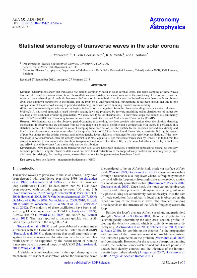
Since 2002, when Ofman & Aschwanden (2002) modelled thescaling relations for standing TLOs, many more observationshave been analysed. Table 1 lists 52 events of TLOs from13 studies. Figure 1 shows the distribution of damping times,τ, versus oscillation period, P. We can find a power-law rela-tionship between those two observed quantities as

τ = α Pγ, log10α = 0.44 ± 0.31, γ = 0.94 ± 0.12. (1)

Under the assumption of a loop where the density drops frominner to external conditions over a thin transition layer, the res-onant absorption rate is given by (e.g. Ionson 1978; Hollweg &Yang 1988; Goossens et al. 1992; Ruderman & Roberts 2002)

τ = ξE P , ξE(�/a, ζ) = F (�/a)−1 ζ + 1ζ − 1

, (2)

where F, �, a and ζ are parameters that describe the cross-sectional profile of the loop mass density, ρ(r). Here, we choosea half-wavelength sinusoidally varying transition layer, i.e.

ρ(r)ρi=

⎧⎪⎪⎪⎨⎪⎪⎪⎩1 r − a < −�/212

[(ζ−1 + 1) + (ζ−1 − 1) sin π(r−a)

�

]|r − a| ≤ �/2

ζ−1 r − a > �/2,

(3)

where ρi is the loop-axis equilibrium density and ζ the ratio ofthe loop-axis density over the external density, i.e. ζ = ρi/ρe.For such a profile, F = 2/π. Equation (2) is, strictly speaking,only valid in the regime where � � a, though Van Doorsselaereet al. (2004) shows that it still provides a relatively accurate ex-tension into the regime of finite resonance layer widths. Also,

Table 1. Characteristics of observed TLOs.

# P (s) τ (s) L(Mm) Reference1

1 261 870 168 A022 265 300 723 316 500 1744 277 400 2045 272 849 1626 435 600 2587 143 200 1668 423 800 4069 185 200 19210 396 400 146

11 234 714 350 ± 50 WS04

12 249 ± 33 920 ± 360 218 V0413 448 ± 18 1260 ± 500 21814 392 ± 31 1830 ± 790 22815 382 ± 12 1330 ± 528 23316 358 ± 30 1030 ± 570 23717 326 ± 45 980 ± 400 23518 357 ± 89 1320 ± 720 236

19 567 1500 400 ± 100 H05 & H0720 918 4200 800 ± 200

21 425 2300 384 VD0722 436 ± 4.5 2129 ± 280 400 ± 4023 243 ± 6.4 1200 400 ± 40

24 895 ± 2 521 ± 8 228 DMB07 & VD0925 452 ± 1 473 ± 6 228

26 630 ± 30 1000 ± 300 340 ± 15 V09

27 2418 ± 5 3660 ± 80 680 ± 50 V10

28 377 500 250 M11

29 225 ± 40 240 ± 45 121 ± 12 WV1230 215 ± 5 293 ± 18 111 ± 1131 213 ± 9 251 ± 36 132 ± 1332 216 ± 27 230 ± 23 113 ± 1133 520 ± 5 735 ± 53 396 ± 4034 596 ± 50 771 ± 336 374 ± 3735 212 ± 20 298 ± 30 279 ± 2836 256 ± 22 444 ± 105 240 ± 2437 135 ± 9 311 ± 85 241 ± 2438 115 ± 2 175 ± 30 159 ± 1639 103 ± 8 242 ± 114 132 ± 13

40 302 ± 14 306 ± 43 466 ± 50 W12

41 565 ± 4 666 ± 42 301 ± 30 V1242 222 ± 18 420 ± 360 274 ± 3043 474 ± 12 900 ± 120 400 ± 3044 1170 ± 6 1218 ± 48 400 ± 3045 623 ± 4 960 ± 60 270 ± 3046 150 ± 5 216 ± 60 188 ± 2047 122 ± 6 348 ± 360 160 ± 2048 273 ± 54 468 ± 36 171 ± 2049 282 ± 6 606 ± 186 122 ± 2050 491 ± 18 834 ± 6 262 ± 2051 348 ± 7 906 ± 288 238 ± 2052 340 ± 3 930 ± 144 200 ± 20

Notes. (1) The reference citations are listed in Fig. 1.

Eq. (2) does not describe any transient behaviour in the damping(Pascoe et al. 2012).

Equation (2) shows that the resonant absorption time-scalescales linearly with period. This matches the observed scalingwell. However, as pointed out by Arregui et al. (2008), a one-to-one comparison is problematic because Eq. (2) also depends

A138, page 2 of 9

E. Verwichte et al.: Statistical seismology of transverse waves in the solar corona

Fig. 1. Damping time versus period of measured TLOs. The thick lineis a power-law fit of the form τ = α Pγ. The parallel lines indicate con-tours of quality factor τ/P. The symbols correspond to the followingpublications reporting TLOs. A02: Aschwanden et al. (2002); WS04:Wang & Solanki (2004); V04: Verwichte et al. (2004); H05: Hori et al.(2005); H07: Hori et al. (2007); VD07: Van Doorsselaere et al. (2007);DMB07: De Moortel & Brady (2007); VD09: Van Doorsselaere et al.(2009); V09: Verwichte et al. (2009), V10: Verwichte et al. (2010);M11: Mrozek (2011); WV12: White & Verwichte (2012); W12: Whiteet al. (2012); V12: Verwichte et al. (2012).

on �/a and ζ, which will vary between loops. We can identify theobserved fit parameter α with ξE(�/a, ζ). What possible range ofvalues of �/a and ζ gives the best match between α and ξE?

2.1. Modelling the damping time-period scaling

To compare theoretical and observed scaling, the followingforward-modelling procedure is adopted. The hidden variablesare allowed to have a distribution of plausible values and are as-sumed to be independent. The distribution of the thickness ofthe inhomogeneity layer, �/a, and the density contrast, ζ, aremodelled as

d(�/a)dN

= H(�/a, (�/a)min, (�/a)max),

dζdN= H(ζ, ζmin, ζmax), (4)

where H(x, xmin, xmax) is the top-hat function defined as

H(x, xmin, xmax) =

{(xmax − xmin)−1 xmin ≤ x ≤ xmax0 x < xmin or x > xmax

· (5)

Alternatively, for ζ, we may also use a Jeffrey’s probability den-sity function, J(x), which is defined as

J(x, xmin, xmax) =

[x ln

(xmax

xmin

)]−1

· (6)

Inherently, the distributions do not depend on other physical pa-rameters or on the period. Thus, we make the assumption thatthe distribution of these parameters is the same for all sizes ofloops. Also, the oscillation period has a distribution

dlog10 P

dN= H(log10 P, log10 Pmax, log10 Pmin), (7)

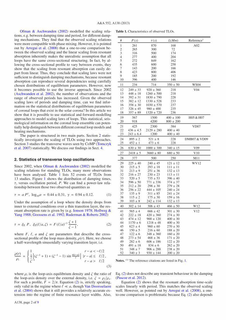
Fig. 2. Example of a realisation of a set of forward-modelled set of(Pi, τi) of the same number as currently reported TLOs. The grey cir-cles indicate a realisation of a 1000 sets. Here, ζ and �/a are sampleduniformly from the intervals [0, 4] and [0, 2], respectively.

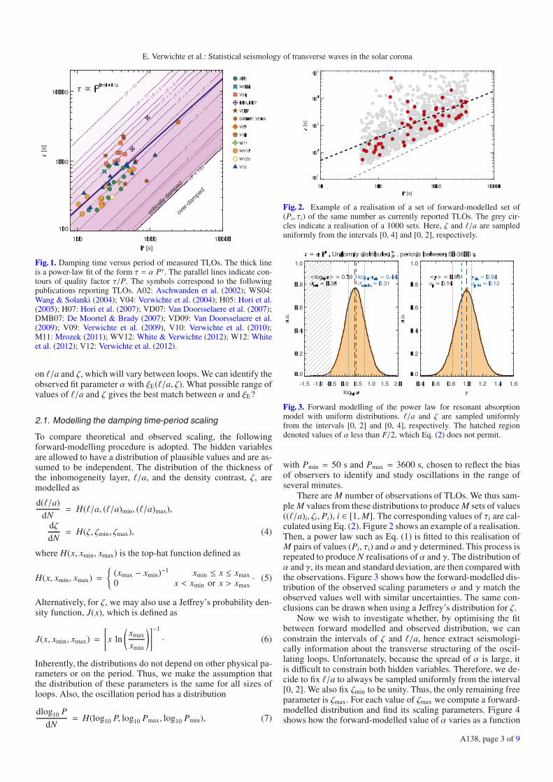
Fig. 3. Forward modelling of the power law for resonant absorptionmodel with uniform distributions. �/a and ζ are sampled uniformlyfrom the intervals [0, 2] and [0, 4], respectively. The hatched regiondenoted values of α less than F/2, which Eq. (2) does not permit.

with Pmin = 50 s and Pmax = 3600 s, chosen to reflect the biasof observers to identify and study oscillations in the range ofseveral minutes.

There are M number of observations of TLOs. We thus sam-ple M values from these distributions to produce M sets of values((�/a)i, ζi, Pi), i ∈ [1,M]. The corresponding values of τi are cal-culated using Eq. (2). Figure 2 shows an example of a realisation.Then, a power law such as Eq. (1) is fitted to this realisation ofM pairs of values (Pi, τi) and α and γ determined. This process isrepeated to produce N realisations of α and γ. The distribution ofα and γ, its mean and standard deviation, are then compared withthe observations. Figure 3 shows how the forward-modelled dis-tribution of the observed scaling parameters α and γ match theobserved values well with similar uncertainties. The same con-clusions can be drawn when using a Jeffrey’s distribution for ζ.

Now we wish to investigate whether, by optimising the fitbetween forward modelled and observed distribution, we canconstrain the intervals of ζ and �/a, hence extract seismologi-cally information about the transverse structuring of the oscil-lating loops. Unfortunately, because the spread of α is large, itis difficult to constrain both hidden variables. Therefore, we de-cide to fix �/a to always be sampled uniformly from the interval[0, 2]. We also fix ζmin to be unity. Thus, the only remaining freeparameter is ζmax. For each value of ζmax we compute a forward-modelled distribution and find its scaling parameters. Figure 4shows how the forward-modelled value of α varies as a function

A138, page 3 of 9

A&A 552, A138 (2013)

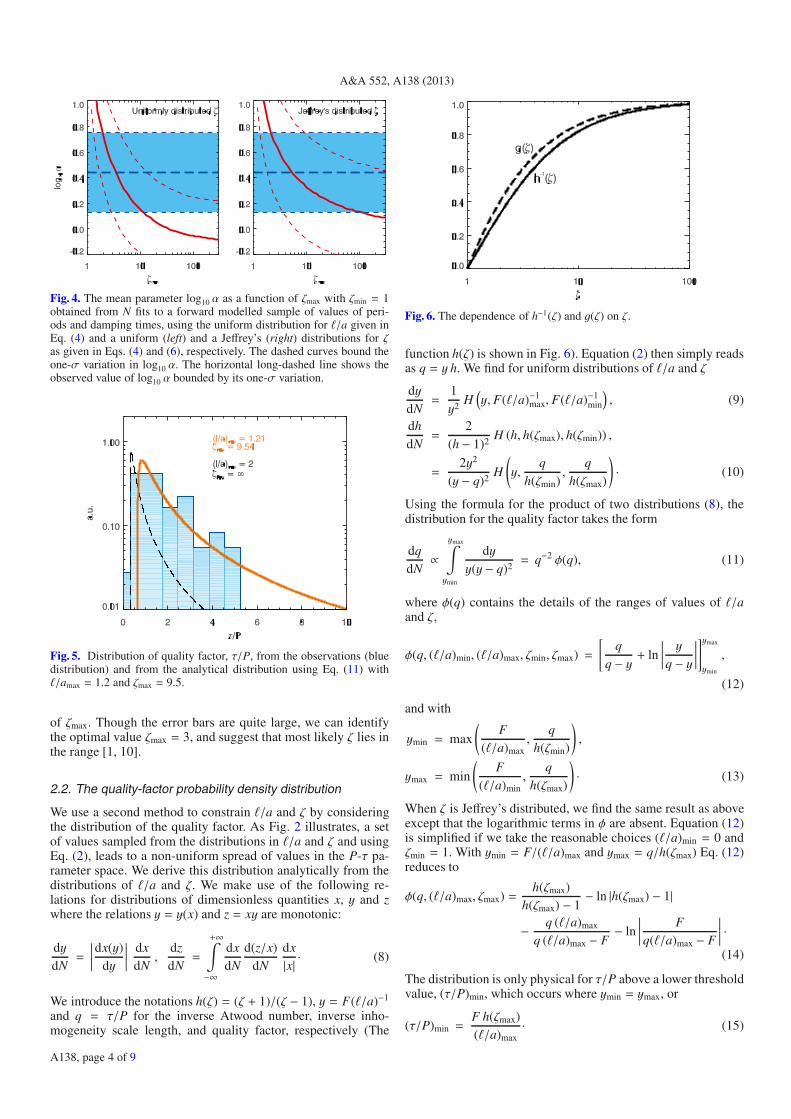
Fig. 4. The mean parameter log10 α as a function of ζmax with ζmin = 1obtained from N fits to a forward modelled sample of values of peri-ods and damping times, using the uniform distribution for �/a given inEq. (4) and a uniform (left) and a Jeffrey’s (right) distributions for ζas given in Eqs. (4) and (6), respectively. The dashed curves bound theone-σ variation in log10 α. The horizontal long-dashed line shows theobserved value of log10 α bounded by its one-σ variation.

Fig. 5. Distribution of quality factor, τ/P, from the observations (bluedistribution) and from the analytical distribution using Eq. (11) with�/amax = 1.2 and ζmax = 9.5.

of ζmax. Though the error bars are quite large, we can identifythe optimal value ζmax = 3, and suggest that most likely ζ lies inthe range [1, 10].

2.2. The quality-factor probability density distribution

We use a second method to constrain �/a and ζ by consideringthe distribution of the quality factor. As Fig. 2 illustrates, a setof values sampled from the distributions in �/a and ζ and usingEq. (2), leads to a non-uniform spread of values in the P-τ pa-rameter space. We derive this distribution analytically from thedistributions of �/a and ζ. We make use of the following re-lations for distributions of dimensionless quantities x, y and zwhere the relations y = y(x) and z = xy are monotonic:

dydN=

∣∣∣∣∣dx(y)dy

∣∣∣∣∣ dxdN,

dzdN=

+∞∫−∞

dxdN

d(z/x)dN

dx|x| · (8)

We introduce the notations h(ζ) = (ζ + 1)/(ζ − 1), y = F(�/a)−1

and q = τ/P for the inverse Atwood number, inverse inho-mogeneity scale length, and quality factor, respectively (The

Fig. 6. The dependence of h−1(ζ) and g(ζ) on ζ.

function h(ζ) is shown in Fig. 6). Equation (2) then simply readsas q = y h. We find for uniform distributions of �/a and ζ

dydN=

1y2

H(y, F(�/a)−1

max, F(�/a)−1min

), (9)

dhdN=

2(h − 1)2

H (h, h(ζmax), h(ζmin)) ,

=2y2

(y − q)2H

(y,

qh(ζmin)

,q

h(ζmax)

)· (10)

Using the formula for the product of two distributions (8), thedistribution for the quality factor takes the form

dqdN∝ymax∫ymin

dyy(y − q)2

= q−2 φ(q), (11)

where φ(q) contains the details of the ranges of values of �/aand ζ,

φ(q, (�/a)min, (�/a)max, ζmin, ζmax) =

[q

q − y + ln∣∣∣∣∣ yq − y

∣∣∣∣∣]ymax

ymin

,

(12)

and with

ymin = max

(F

(�/a)max,

qh(ζmin)

),

ymax = min

(F

(�/a)min,

qh(ζmax)

)· (13)

When ζ is Jeffrey’s distributed, we find the same result as aboveexcept that the logarithmic terms in φ are absent. Equation (12)is simplified if we take the reasonable choices (�/a)min = 0 andζmin = 1. With ymin = F/(�/a)max and ymax = q/h(ζmax) Eq. (12)reduces to

φ(q, (�/a)max, ζmax) =h(ζmax)

h(ζmax) − 1− ln |h(ζmax) − 1|

− q (�/a)max

q (�/a)max − F− ln

∣∣∣∣∣ Fq(�/a)max − F

∣∣∣∣∣ ·(14)

The distribution is only physical for τ/P above a lower thresholdvalue, (τ/P)min, which occurs where ymin = ymax, or

(τ/P)min =F h(ζmax)(�/a)max

· (15)

A138, page 4 of 9

E. Verwichte et al.: Statistical seismology of transverse waves in the solar corona

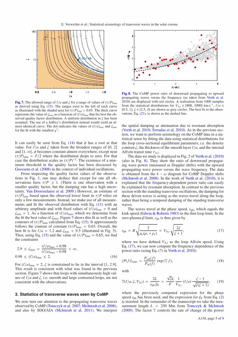
Fig. 7. The allowed range of �/a and ζ for a range of values of (τ/P)min

as derived using Eq. (15). The ranges exist to the left of each curveas illustrated with the shaded area for (τ/P)min = 0.65. The thick curverepresents the value of ζmax as a function of (�/a)max that fits best the ob-served quality factor distribution. A uniform distribution in ζ has beenassumed. The use of a Jeffrey’s distribution instead would yield an al-most identical curve. The dot indicates the values of (�/a)max and ζmax

for the fit with the smallest χ2.

It can easily be seen from Eq. (14) that φ has a root at thatvalue. For �/a and ζ taken from the broadest ranges of [0, 2]and [1,∞[, φ becomes constant almost everywhere, except near(τ/P)min = F/2 where the distribution drops to zero. For thatcase the distribution scales as (τ/P)−2. The existence of a min-imum threshold in the quality factor has been discussed byGoossens et al. (2008) in the context of individual oscillations.

From inspecting the quality factor values of the observa-tions in Fig. 1, one may deduce that except for one all ob-servations have τ/P ≥ 1. (There is one observation with asmaller quality factor, but the damping rate has a high uncer-tainty, Van Doorsselaere et al. 2009.) However, an estimate of(τ/P)min based upon the observed lower limit in τ/P relies ononly a few measurements. Instead, we make use of all measure-ments and fit the observed distribution with Eq. (11) with anarbitrary amplitude and with fixed values of (�/a)min = 0 andζmin = 1. As a function of (�/a)max, which we determine fromthe fit the best value of ζmax. Figure 7 shows this fit as well as thecontours of (τ/P)min calculated from Eq. (15). It approximatelyfollows the contour of constant (τ/P)min = 0.65. Overall, thebest fit is for �/a = 1.2 and ζmax = 9.5 (illustrated in Fig. 5).Then, using Eq. (15) and the value of (τ/P)min = 0.65, we findthe constraints

2.9 ≤ ζmax =(�/a)max + 0.98(�/a)max − 0.98

< ∞,0.98 ≤ (�/a)max ≤ 2. (16)

For (�/a)max = 2, ζ is constrained to lie in the interval [1, 2.9].This result is consistent with what was found in the previoussection. Figure 7 shows that loops with simultaneously high val-ues of �/a and ζ, i.e. smooth and large contrasted loops, are notconsistent with the observations.

3. Statistics of transverse waves seen by CoMP

We now turn our attention to the propagating transverse wavesobserved by CoMP (Tomczyk et al. 2007; McIntosh et al. 2008),and also by SDO/AIA (McIntosh et al. 2011). We interpret

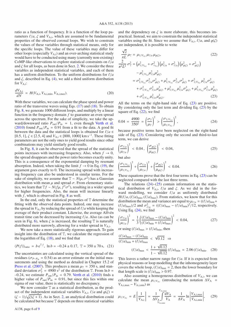
Fig. 8. The CoMP power ratio of downward propagating to upwardpropagating waves versus the frequency (as taken from Verth et al.2010) are displayed with red circles. A realisation from 1000 samplesfrom the statistical distributions for VA,i ∈ [800, 1000] km s−1, �/a ∈[0.5, 1], ζ ∈ [2.5, 4] are shown as grey circles. The best fit to the obser-vations, Eq. (21), is shown as the dashed line.

the spatial damping as attenuation due to resonant absorption(Verth et al. 2010; Terradas et al. 2010). As in the previous sec-tion, we want to perform seismology on the CoMP data in a sta-tistical sense by fitting the data using statistical distributions forthe loop cross-sectional equilibrium parameters, i.e. the densitycontrast ζ, the thickness of the smooth layer �/a, and the internalAlfvén transit time τA,i.

The data we study is displayed in Fig. 2 of Verth et al. (2010)(also in Fig. 8). They show the ratio of downward propagat-ing wave power (measured as Doppler shifts) with the upwardpropagating wave power versus the wave frequency. The datais obtained from the k − ω diagram for CoMP Doppler shifts(McIntosh et al. 2008). In the work of Verth et al. (2010), it isexplained that the frequency-dependent power ratio can easilybe explained by resonant absorption. In contrast to the previoussection with the standing transverse oscillations, the damping forthese driven waves is acting as the waves travel along the loop,rather than being a temporal damping of the standing transversewaves.

The waves travel at the phase speed, vph, which equals thekink speed (Edwin & Roberts 1983) in the thin loop limit. In thezero plasma-β limit, vph is thus given by

vph = B

√2

μo(ρi + ρe)= VA,i

√2ζζ + 1

, (17)

where we have defined VA,i as the loop Alfvén speed. UsingEq. (17), we can now compute the frequency dependence of thepower ratio (using Eq. (7) in Verth et al. 2010):

〈P( f )〉ratio =Pout( f )Pin( f )

exp (T f ), (18)

with

T(�/a, ζ,VA,i) =2Lvph ξE

=

√2LF

1VA,i

(�/a)ζ − 1√ζ(ζ + 1)

, (19)

where the previously computed expression for the phasespeed vph has been used, and the expression for ξE from Eq. (2)is inserted. In the remainder of the manuscript we take the mea-surement length L = 250 Mm from Tomczyk & McIntosh(2009). The factor T controls the rate of change of the power

A138, page 5 of 9

A&A 552, A138 (2013)

ratio as a function of frequency. It is a function of the loop pa-rameters �/a, ζ and VA,i, which are assumed to be fundamentalproperties of the observed coronal loops. We wish to constrainthe values of these variables through statistical means, only forthe specific loops. The value of these variables may differ forother loops (especially VA,i) and an over-arching statistical studywould have to be conducted using many (currently non-existing)CoMP-like observations to explore statistical constraints on �/aand ζ for all loops, as been done in Sect. 2. We consider the threevariables as independent statistical variables, and each of themhas a uniform distribution. To the uniform distributions for �/aand ζ, described in Eq. (4), we add a third uniform distributionfor VA,i:

dVA,i

dN= H(VA,i,VA,i,min,VA,i,max). (20)

With these variables, we can calculate the phase speed and powerratio of the transverse waves using Eqs. (17) and (18). To obtainFig. 8, we generate 1000 different loops, and multiply by a linearfunction in the frequency domain f to guarantee an even spreadacross the spectrum. For the sake of simplicity, we take the up-ward/downward ratio Pout/Pin = 1, even though Verth et al.(2010) found Pout/Pin = 0.91 from a fit to the data. A good fitbetween the data and the statistical loops is obtained for �/a ∈[0.5, 1], ζ ∈ [2.5, 4] and VA,i ∈ [800, 1000] km s−1. These fittingparameters are not the only ones to yield good results since othercombinations may yield similarly good results.

In Fig. 8, it can be observed that the spread of the statisticalpoints increases with increasing frequency. Also, when f → 0,the spread disappears and the power ratio becomes exactly unity.This is a consequence of the exponential damping by resonantabsorption. Indeed, when taking the limit f → 0 in Eq. (19), theargument goes exactly to 0. The increasing spread with increas-ing frequency can also be understood in similar terms. For thesake of simplicity, we assume that T ∼ N(μ, σ2) has a Gaussiandistribution with mean μ and spread σ. From elementary statis-tics, we learn that T f ∼ N( fμ, f 2σ2), resulting in a wider spreadfor higher frequencies. Also, the mean will increase linearlywith f , which is observed in Fig. 8 as well.

In the end, only the statistical properties of T determine thefitting with the observed data points. Indeed, one may increasethe spread in VA,i by reducing the spread of �/a while keeping theaverage of their product constant. Likewise, the average Alfvéntransit time can be decreased by increasing �/a. Also (as can beseen in Fig. 6), when ζ is increased, the resulting T is naturallydistributed more narrowly, allowing for a wider spread in VA,i.

We now take a more statistically rigorous approach. To gaininsight into the distribution of T, we calculate the regression ofthe logarithm of Eq. (18), and we find that

〈P( f )〉ratio = b eT f , ln b = −0.24 ± 0.17, T = 350 ± 70 s, (21)

The uncertainties are calculated using the vertical spread of theresidues (σP−Pfit = 0.54) as an error estimate on the initial mea-surements and using the method as detailed in Chapter 15.2 ofPress et al. (2007). This produces a mean μT = 350 s, and stan-dard deviation σ2

T= 4900 s2 of the distribution T. From ln b =

–0.24, we estimate Pout/Pin = 0.79. Verth et al. (2010) finds ahigher value of Pout/Pin = 0.91, but since this lies within onesigma of our value, there is statistically no discrepancy.

We now consider T as a statistical distribution, as the prod-uct of the independent statistical variables VA,i, �/a and g(ζ) =(ζ − 1)/

√ζ(ζ + 1). As in Sect. 2, an analytical distribution could

be calculated but because T depends on three statistical variables

and the dependency on ζ is more elaborate, this becomes im-practical. Instead, we aim to constrain the independent statisticalvariables using the fit. Since we assume that VA,i, �/a, and g(ζ)are independent, it is possible to write√

2πLμT = μ1/VA,i μ�/a μg(ζ), (22)

2π2L2

σ2T=

(μ2

1/VA,i+ σ2

τA,i

) (μ2�/a + σ

2�/a

) (μ2g(ζ) + σ

2g(ζ)

)− μ2

1/VA,iμ2�/aμ

2g(ζ)

= σ21/VA,iσ2�/aσ

2g(ζ) + μ

21/VA,iσ2�/aσ

2g(ζ) + σ

21/VA,iμ2�/aσ

2g(ζ)

+ σ21/VA,iσ2�/a μ

2g(ζ) + μ

21/VA,iμ2�/aσ

2g(ζ) + μ

21/VA,iσ2�/a μ

2g(ζ)

+ σ21/VA,iμ2�/a μ

2g(ζ). (23)

All the terms on the right-hand side of Eq. (23) are positive.By considering only the last term and dividing Eq. (23) by thesquare of Eq. (22), we find

0.04 =49003502

=

(σTμT

)2

>

(σ1/VA,i

μ1/VA,i

)2

, (24)

because positive terms have been neglected on the right-handside of Eq. (23). Considering only the second and third-to-lastterm, we can derive(σ�/a

μ�/a

)2

< 0.04 ,

(σg(ζ)

μg(ζ)

)2

< 0.04, (25)

but also(σ1/VA,i

μ1/VA,i

)2

+

(σ�/a

μ�/a

)2

+

(σg(ζ)

μg(ζ)

)2

< 0.04. (26)

These equations prove that the first four terms in Eq. (23) can beneglected compared with the last three terms.

The relations (24)–(25) contain information on the statis-tical distribution of VA,i, �/a and ζ. As we did in the for-ward modelling, we consider �/a as uniformly distributedH(�/a, (�/a)min, (�/a)max). From statistics, we know that for thisdistribution the mean and variance are equal to μ�/a = ((�/a)min+(�/a)max)/2 and σ2

�/a = ((�/a)max − (�/a)min)2/12, respectively.Using Eq. (24), we find(σ�/a

μ�/a

)2

=13

((�/a)max − (�/a)min

(�/a)min + (�/a)max

)2

< 0.04, (27)

or using (�/a)max > (�/a)min, then

(�/a)max − (�/a)min

(�/a)min + (�/a)max<√

0.12 ⇒

(�/a)max <1 +√

0.12

1 − √0.12(�/a)min = 2.06 (�/a)min. (28)

This leaves a rather narrow range for �/a. If it is expected fromphysical reasons or loop modelling that the inhomogeneity layercovers the whole loop, (�/a)max = 2, then the lower boundary forthat length scale is (�/a)min > 0.97.

Also assuming a homogeneous distribution of VA,i, we cancalculate the mean μ1/VA,i (introducing the notation ΔVA =VA,i,max − VA,i,min) as

μ1/VA,i = E

[1

VA,i

]=

1ΔVA

VA,i,max∫VA,i,min

dVA

VA=

1ΔVA

ln

∣∣∣∣∣∣VA,i,max

VA,i,min

∣∣∣∣∣∣, (29)

A138, page 6 of 9

E. Verwichte et al.: Statistical seismology of transverse waves in the solar corona

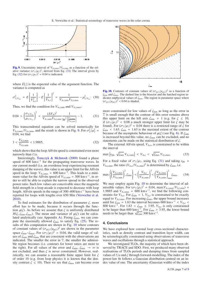
Fig. 9. Uncertainty interval of VA,i,max/VA,i,min as a function of the rel-ative variance (σT/μT)2, derived from Eq. (31) The interval given byEq. (32) for (σT/μT)2 = 0.04 is indicated.

where E[.] is the expected value of the argument function. Thevariance is computed as

σ21/VA,i

= E

⎡⎢⎢⎢⎢⎢⎣ 1

V2A,i

⎤⎥⎥⎥⎥⎥⎦ − E

[1

VA,i

]2

=1

VA,i,minVA,i,max− μ2

1/VA,i· (30)

Thus, we find the condition for VA,i,min and VA,i,max:

0.04 >

(σ1/VA,i

μ1/VA,i

)2

=(ΔVA)2

VA,i,minVA,i,max

1

ln2∣∣∣∣VA,i,max

VA,i,min

∣∣∣∣ − 1. (31)

This transcendental equation can be solved numerically forVA,i,max/VA,i,min, and the result is shown in Fig. 9. For σ2

T/μ2T=

0.04, we find

1 <VA,i,max

VA,i,min< 1.9885, (32)

which shows that the loop Alfvén speed is constrained even morenarrowly than �/a.

Interestingly, Tomczyk & McIntosh (2009) found a phasespeed of 600 km s−1 for the propagating transverse waves. Inour current model (i.e. an overdense loop experiencing resonantdamping of the waves), this value is an upper limit for the Alfvénspeed in the loop: VA,i,max = 600 km s−1. This leads to a mini-mum value for the Alfvén speed of VA,i,min = 300 km s−1, in or-der to still be able to explain the narrow spread in the observedpower ratio. Such low values are conceivable since the magneticfield strength in a loop arcade is expected to decrease with looplength. Alfvén speeds in the range of 300–400 km s−1 have beenreported for loops with lengths over 650 Mm (Verwichte et al.2010).

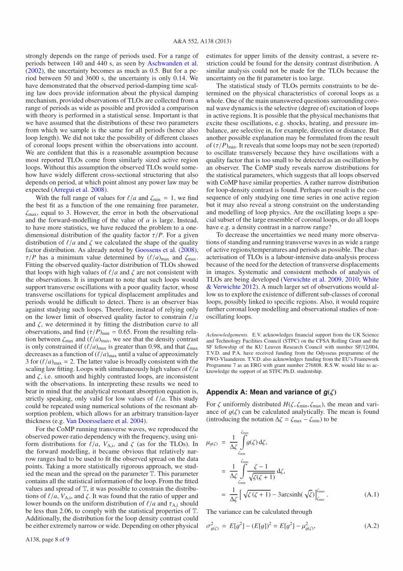
To find estimates for the distribution of parameter ζ, moreeffort has to be made, because it occurs through the func-tion g(ζ). As before we assume that ζ is uniformly distributedH(ζ, ζmin, ζmax). The mean and variance of g(ζ) can be calcu-lated analytically (see Appendix A). Fixing ζmin, we can com-pute the maximally allowed ζmax to satisfy Eq. (25). The re-sults of this computation are shown in Fig. 10 where contoursof constant values of (σg(ζ)/μg(ζ))2 are shown in the parameterspace ζmin−ζmax. For (σT/μT)2 = 0.04, the valid range of val-ues of ζmin and ζmax that are consistent with the observations areindicated. The smaller the error in T, the smaller the admissi-ble region becomes (i.e. contours for lower ratios are more tothe right). For all values of the error and ζmin, ζmax → ∞ isnot excluded, and thus ζ is never constrained. However, real-istically, we can assume a reasonable finite upper limit for ζof order 10 (e.g. from loop physics it is known that the den-sity contrast ζ ≤ 10). Then we see that ζmax can become even

Fig. 10. Contours of constant values of (σg(ζ)/μg(ζ))2 as a function ofζmin and ζmax. The dashed line is the bisector and the hatched region in-dicates unphysical values of ζmax. The region in parameter space where(σg(ζ)/μg(ζ))2 < 0.04 is shaded.

more constrained for low values of ζmin as long as the error inT is small enough that the contour of this error remains abovethis upper limit on the left axis ζmin = 1 (e.g. for ζ ≤ 10,if (σT/μT)2 < 0.08 a much stronger upper limit for ζ may befound). For (σT/μT)2 = 0.04 there is a restricted range of ζ forζmin < 1.63. ζmin = 1.63 is the maximal extent of the contourbecause of the asymptotic behaviour of g(ζ) (see Fig. 6). If ζminis increased beyond this value, no ζmax can be excluded, and nostatements can be made on the statistical distribution of ζ.

The external Alfvén speed, VA,e, is constrained to be withinthe interval

max{vph,

√ζmin VA,i,min

}< VA,e <

√ζmax VA,i,max. (33)

For a fixed value of σT/μT, using Eq. (31) and taking vph =

VA,i,min, the ratio (VA,e/VA,i,min)2 is determined by ζmin, i.e.

max

⎧⎪⎪⎨⎪⎪⎩(VA,i,max

VA,i,min

)2

, ζmin

⎫⎪⎪⎬⎪⎪⎭ <(

VA,e

VA,i,min

)2

<

(VA,i,max

VA,i,min

)2

max

ζmax. (34)

We may employ again Fig. 10 to determine the interval of ad-missible values. For (σT/μT)2 = 0.04, max(VA,i,max/VA,i,min) =1.9885 and VA,i,max = 600 km s−1, we find the following con-straints for VA,e. For ζmin = 1, VA,e is constrained to be exactlyequal to VA,i,max. For increasing ζmin, the upper bound increasesuntil for ζmin = 1.63 the interval becomes 600 km s−1 < VA,e <800 km s−1. For 1.63 < ζmin ≤ 3.95, VA,e is only constrainedto be larger than 600 km s−1. For ζmin > 3.95, the lower boundneeds to be larger than

√ζmin 300 km s−1.

4. Conclusions

We have explored how coronal loop cross-sectional character-istics, such as density contrast and transition layer width, canbe seismologically constrained using observations of transversewaves and oscillations through a statistical approach.

We investigated TLOs, the majority of which have been ob-served by TRACE and SDO. First, we produced many observedrealisations of TLOs periods and damping times from sampledvalues of �/a and ζ through forward-modelling. The index of thepower-law fit follows a Gaussian distribution centred on an in-dex value of one. The uncertainty (Gaussian width) of the index

A138, page 7 of 9

A&A 552, A138 (2013)

strongly depends on the range of periods used. For a range ofperiods between 140 and 440 s, as seen by Aschwanden et al.(2002), the uncertainty becomes as much as 0.5. But for a pe-riod between 50 and 3600 s, the uncertainty is only 0.14. Wehave demonstrated that the observed period-damping time scal-ing law does provide information about the physical dampingmechanism, provided observations of TLOs are collected from arange of periods as wide as possible and provided a comparisonwith theory is performed in a statistical sense. Important is thatwe have assumed that the distributions of these two parametersfrom which we sample is the same for all periods (hence alsoloop length). We did not take the possibility of different classesof coronal loops present within the observations into account.We are confident that this is a reasonable assumption becausemost reported TLOs come from similarly sized active regionloops. Without this assumption the observed TLOs would some-how have widely different cross-sectional structuring that alsodepends on period, at which point almost any power law may beexpected (Arregui et al. 2008).

With the full range of values for �/a and ζmin = 1, we findthe best fit as a function of the one remaining free parameter,ζmax, equal to 3. However, the error in both the observationaland the forward-modelling of the value of α is large. Instead,to have more statistics, we have reduced the problem to a one-dimensional distribution of the quality factor τ/P. For a givendistribution of �/a and ζ we calculated the shape of the qualityfactor distribution. As already noted by Goossens et al. (2008),τ/P has a minimum value determined by (�/a)max and ζmax.Fitting the observed quality-factor distribution of TLOs showedthat loops with high values of �/a and ζ are not consistent withthe observations. It is important to note that such loops wouldsupport transverse oscillations with a poor quality factor, whosetransverse oscillations for typical displacement amplitudes andperiods would be difficult to detect. There is an observer biasagainst studying such loops. Therefore, instead of relying onlyon the lower limit of observed quality factor to constrain �/aand ζ, we determined it by fitting the distribution curve to allobservations, and find (τ/P)min = 0.65. From the resulting rela-tion between ζmax and (�/a)max, we see that the density contrastis only constrained if (�/a)max is greater than 0.98, and that ζmaxdecreases as a function of (�/a)max until a value of approximately3 for (�/a)max = 2. The latter value is broadly consistent with thescaling law fitting. Loops with simultaneously high values of �/aand ζ, i.e. smooth and highly contrasted loops, are inconsistentwith the observations. In interpreting these results we need tobear in mind that the analytical resonant absorption equation is,strictly speaking, only valid for low values of �/a. This studycould be repeated using numerical solutions of the resonant ab-sorption problem, which allows for an arbitrary transition-layerthickness (e.g. Van Doorsselaere et al. 2004).

For the CoMP running transverse waves, we reproduced theobserved power-ratio dependency with the frequency, using uni-form distributions for �/a, VA,i, and ζ (as for the TLOs). Inthe forward modelling, it became obvious that relatively nar-row ranges had to be used to fit the observed spread on the datapoints. Taking a more statistically rigorous approach, we stud-ied the mean and the spread on the parameter T. This parametercontains all the statistical information of the loop. From the fittedvalues and spread of T, it was possible to constrain the distribu-tions of �/a, VA,i, and ζ. It was found that the ratio of upper andlower bounds on the uniform distribution of �/a and τA,i shouldbe less than 2.06, to comply with the statistical properties of T.Additionally, the distribution for the loop density contrast couldbe either extremely narrow or wide. Depending on other physical

estimates for upper limits of the density contrast, a severe re-striction could be found for the density contrast distribution. Asimilar analysis could not be made for the TLOs because theuncertainty on the fit parameter is too large.

The statistical study of TLOs permits constraints to be de-termined on the physical characteristics of coronal loops as awhole. One of the main unanswered questions surrounding coro-nal wave dynamics is the selective (degree of) excitation of loopsin active regions. It is possible that the physical mechanisms thatexcite these oscillations, e.g. shocks, heating, and pressure im-balance, are selective in, for example, direction or distance. Butanother possible explanation may be formulated from the resultof (τ/P)min. It reveals that some loops may not be seen (reported)to oscillate transversely because they have oscillations with aquality factor that is too small to be detected as an oscillation byan observer. The CoMP study reveals narrow distributions forthe statistical parameters, which suggests that all loops observedwith CoMP have similar properties. A rather narrow distributionfor loop-density contrast is found. Perhaps our result is the con-sequence of only studying one time series in one active regionbut it may also reveal a strong constraint on the understandingand modelling of loop physics. Are the oscillating loops a spe-cial subset of the large ensemble of coronal loops, or do all loopshave e.g. a density contrast in a narrow range?

To decrease the uncertainties we need many more observa-tions of standing and running transverse waves in as wide a rangeof active regions/temperatures and periods as possible. The char-acterisation of TLOs is a labour-intensive data-analysis processbecause of the need for the detection of transverse displacementsin images. Systematic and consistent methods of analysis ofTLOs are being developed (Verwichte et al. 2009, 2010; White& Verwichte 2012). A much larger set of observations would al-low us to explore the existence of different sub-classes of coronalloops, possibly linked to specific regions. Also, it would requirefurther coronal loop modelling and observational studies of non-oscillating loops.

Acknowledgements. E.V. acknowledges financial support from the UK Scienceand Technology Facilities Council (STFC) on the CFSA Rolling Grant and theSF fellowship of the KU Leuven Research Council with number SF/12/004,T.V.D. and P.A. have received funding from the Odysseus programme of theFWO-Vlaanderen. T.V.D. also acknowledges funding from the EU’s FrameworkProgramme 7 as an ERG with grant number 276808. R.S.W. would like to ac-knowledge the support of an STFC Ph.D. studentship.

Appendix A: Mean and variance of g(ζ)

For ζ uniformly distributed H(ζ, ζmin, ζmax), the mean and vari-ance of g(ζ) can be calculated analytically. The mean is found(introducing the notation Δζ = ζmax − ζmin) to be

μg(ζ) =1Δζ

ζmax∫ζmin

g(ζ) dζ,

=1Δζ

ζmax∫ζmin

ζ − 1√ζ(ζ + 1)

dζ,

=1Δζ

[ √ζ (ζ + 1) − 3arcsinh(

√ζ)

]ζmax

ζmin. (A.1)

The variance can be calculated through

σ2g(ζ) = E[g2] − (E[g])2 = E[g2] − μ2

g(ζ), (A.2)

A138, page 8 of 9

E. Verwichte et al.: Statistical seismology of transverse waves in the solar corona

where E[.] stands for the expected value of the argument func-tion. For g(ζ), we find

E[g2] =1Δζ

ζmax∫ζmin

g2(ζ) dζ,

=1Δζ

ζmax∫ζmin

(ζ − 1)2

ζ(ζ + 1)dζ,

=1Δζ

[ζ + ln (ζ) − 4 ln (ζ + 1)

]ζmax

ζmin, (A.3)

which is combined with Eq. (A.1) to compute Eq. (A.2).

References

Arregui, I., & Asensio Ramos, A. 2011, ApJ, 740, 44Arregui, I., Andries, J., Van Doorsselaere, T., Goossens, M., & Poedts, S. 2007,

A&A, 463, 333Arregui, I., Ballester, J. L., & Goossens, M. 2008, ApJ, 676, L77Aschwanden, M. J., Fletcher, L., Schrijver, C. J., & Alexander, D. 1999, ApJ,

520, 880Aschwanden, M. J., de Pontieu, B., Schrijver, C. J., & Title, A. M. 2002,

Sol. Phys., 206, 99Aschwanden, M. J., Nightingale, R. W., Andries, J., Goossens, M., &

Van Doorsselaere, T. 2003, ApJ, 598, 1375De Moortel, I., & Brady, C. S. 2007, ApJ, 664, 1210Edwin, P. M., & Roberts, B. 1983, Sol. Phys., 88, 179Goossens, M., Hollweg, J. V., & Sakurai, T. 1992, Sol. Phys., 138, 233Goossens, M., Andries, J., & Aschwanden, M. J. 2002, A&A, 394, L39Goossens, M., Arregui, I., Ballester, J. L., & Wang, T. J. 2008, A&A, 484, 851Goossens, M., Andries, J., Soler, R., et al. 2012, ApJ, 753, 111Handy, B. N., Acton, L. W., Kankelborg, C. C., et al. 1999, Sol. Phys., 187, 229Hollweg, J. V., & Yang, G. 1988, J. Geophys. Res., 93, 5423Hori, K., Ichimoto, K., Sakurai, T., Sano, I., & Nishino, Y. 2005, ApJ, 618, 1001

Hori, K., Ichimoto, K., & Sakurai, T. 2007, in New Solar Physics with Solar-BMission, eds. K. Shibata, S. Nagata, & T. Sakurai, ASP Conf. Ser., 369, 213

Howard, R. A., Moses, J. D., Vourlidas, A., et al. 2008, Space Sci. Rev., 136, 67Ionson, J. A. 1978, ApJ, 226, 650Lemen, J. R., Title, A. M., Akin, D. J., et al. 2012, Sol. Phys., 275, 17McIntosh, S. W., de Pontieu, B., & Tomczyk, S. 2008, Sol. Phys., 252, 321McIntosh, S. W., de Pontieu, B., Carlsson, M., et al. 2011, Nature, 475, 477Mrozek, T. 2011, Sol. Phys., 270, 191Nakariakov, V. M., & Ofman, L. 2001, A&A, 372, L53Nakariakov, V. M., Ofman, L., Deluca, E. E., Roberts, B., & Davila, J. M. 1999,

Science, 285, 862Ofman, L., & Aschwanden, M. J. 2002, ApJ, 576, L153Pascoe, D. J., Hood, A. W., de Moortel, I., & Wright, A. N. 2012, A&A, 539,

A37Press, W. H., Teukolsky, S. A., Vetterling, W. T., & Flannery, B. P. 2007,

Numerical Recipes: The Art of Scientific ComputingRuderman, M. S., & Roberts, B. 2002, ApJ, 577, 475Schmelz, J. T., Beene, J. E., Nasraoui, K., et al. 2003, ApJ, 599, 604Terradas, J., Goossens, M., & Verth, G. 2010, A&A, 524, A23Terzo, S., & Reale, F. 2010, A&A, 515, A7Tomczyk, S., & McIntosh, S. W. 2009, ApJ, 697, 1384Tomczyk, S., McIntosh, S. W., Keil, S. L., et al. 2007, Science, 317, 1192Tomczyk, S., Card, G. L., Darnell, T., et al. 2008, Sol. Phys., 247, 411Van Doorsselaere, T., Andries, J., Poedts, S., & Goossens, M. 2004, ApJ, 606,

1223Van Doorsselaere, T., Nakariakov, V. M., & Verwichte, E. 2007, A&A, 473, 959Van Doorsselaere, T., Birtill, D. C. C., & Evans, G. R. 2009, A&A, 508, 1485Verth, G., Terradas, J., & Goossens, M. 2010, ApJ, 718, L102Verwichte, E., Nakariakov, V. M., Ofman, L., & Deluca, E. E. 2004, Sol. Phys.,

223, 77Verwichte, E., Foullon, C., & Nakariakov, V. M. 2006, A&A, 452, 615Verwichte, E., Aschwanden, M. J., Van Doorsselaere, T., Foullon, C., &

Nakariakov, V. M. 2009, ApJ, 698, 397Verwichte, E., Foullon, C., & Van Doorsselaere, T. 2010, ApJ, 717, 458Verwichte, E., Van Doorsselaere, T., White, R., Bacon, A., & Williams, A. 2012,

A&AWang, T. J., & Solanki, S. K. 2004, A&A, 421, L33Wang, T., Ofman, L., Davila, J. M., & Su, Y. 2012, ApJ, 751, L27Wentzel, D. G. 1979, ApJ, 227, 319White, R. S., & Verwichte, E. 2012, A&A, 537, A49White, R. S., Verwichte, E., & Foullon, C. 2012, A&A, 545, A129

A138, page 9 of 9