statistical mechanics: an overvie · chapter 1 statistical mechanics: an overview 1.1 introduction...

Chapter 1

Statistical Mechanics: An overview

1.1 Introduction

Thermodynamics deals with the thermal properties of macroscopic system by deter-mining the relationship between different thermodynamic parameters of the system.In order to determine different relationships between the system parameters, the in-ternal structure of matter is completely ignored in thermodynamics. The motion ofatoms, molecules or ions of a system, their interactions with each other or with theexternal field are not considered in this subject. Thermodynamics is purely basedon principles formulated by generalizing experimental observations. On the otherhand, statistical mechanics describes the thermodynamic behaviour of macroscopicsystems from the laws which govern the behaviour of the constituent elements at themicroscopic level. In the formalism of statistical mechanics, a macroscopic propertyof a system is obtained by taking a “statistical average” (or “ensemble average”) ofthe property over all possible “microstates” of the system at thermodynamic equi-librium. A microstate of a system is defined by specifying the states of all of itsconstituent elements. Below, a brief statistical mechanical description of fluid andmagnetic systems will be given.

A macroscopic therodynamic system, generally, is composed of a large number (ofthe order of Avogadro number NA ≈ 6.022×1023 per mole) of microscopic elementssuch as atoms, molecules, dipole moments or magnetic moments, etc. Each elementmay have a large number of internal degrees of freedom associated with differenttypes of motion such as translation, rotation, vibration etc. The constituent elementsusually interact among each other via certain complex interactions. They may aswell interact with the external fields applied to the system. In the thermodynamic

limit, the macroscopic properties of a thermodynamic system is thus determinedby the properties of the constituent molecules, their internal interactions as well asinteraction with external fields.

The thermodynamic limit of a macroscopic system of density ρ with volume V and

1

Chapter 1. Statistical Mechanics: An overview

number of elements N is defined as

limN → ∞ limV → ∞ but ρ =N

V= finite. (1.1)

In this limit, the extensive parameters (such as volume, entropy, etc.) of the systembecome directly proportional to the size of the system (N or V ), while the intensiveparameters (such as pressure, teperature, external field, etc.) become independentof the size of the system.

1.2 Specification of microstates

The macroscopic state of a thermodynamic system at equilibrium is specified bythe values of a set of measurable thermodynamic parameters. For example, themacrostate of a fluid system can be specified by pressure P , temperature T andvolume V . For a magnetic system it can be described by external magnetic fieldB, magnetization M and temperature T . A microstate of a system, on the otherhand, is obtained by specifying the states of all of its constituent elements. However,it depends on the nature of the constituent elements (or particles) of the system.Specification of microstates are made differently for classical and quantum particles.We will describe both the situations below.

Microstates of classical particles: In order to specify the microstates of a systemof classical particles, one needs to specify the position q and the conjugate momen-tum p of each and every constituent particle of the system. In a classical system,the time evolution of q and p is governed by the classical Hamiltonian H(p, q) andHamilton’s equation of motion

qi =∂H (p, q)

∂piand pi = −∂H (p, q)

∂qi, i = 1, 2, 3, · · · , 3N (1.2)

for a system of N particles in 3-dimensions. The state of a single particle at any timeis then given by the pair of conjugate variables (qi, pi), a point in the phase space.Each single particle then constitutes a 6-dimensional phase space (3-coordinate and3-momentum). For N particles, the state of the system is then completely anduniquely defined by 3N canonical coordinates q1, q2, · · · , q3N and 3N canonical mo-ment p1, p, · · · , p3N . These 6N variables constitute a 6N -dimensional Γ-space orphase space of the system and each point of the phase space represents a mi-crostate of the system. The locus of all the points in Γ-space satisfying the conditionH(p, q) = E, total energy of the system, defines the energy surface.

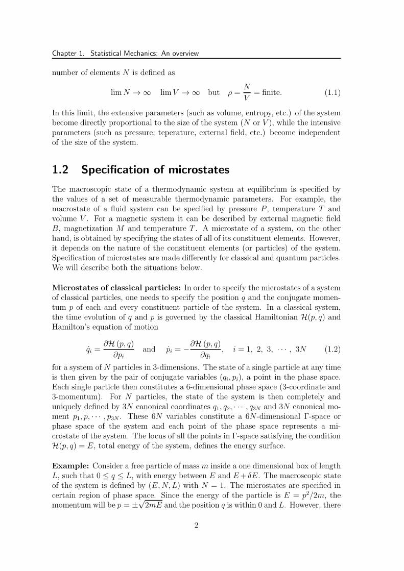
Example: Consider a free particle of mass m inside a one dimensional box of lengthL, such that 0 ≤ q ≤ L, with energy between E and E+ δE. The macroscopic stateof the system is defined by (E,N, L) with N = 1. The microstates are specified incertain region of phase space. Since the energy of the particle is E = p2/2m, themomentum will be p = ±

√2mE and the position q is within 0 and L. However, there

2

1.2 Specification of microstates

(a) (b)

Figure 1.1: (a) Accessible region of phase space for a free particle of mass m and energyE in a one dimensional box of length L. (b) Region of phase space for a one dimensionalharmonic oscillator with energy E, mass m and spring constant k.

is a small width in energy δE, so the particles are confined in small strips of widthδp =

√

m/2EδE as shown in Fig.1.1(a). Note that if δE = 0, the accessible region ofphase space representing the system would be one dimensional in a two dimensionalphase space. In order to avoid this artifact a small width in E is considered whichdoes not affect the final results in the thermodynamic limit. In Fig.1.1(b), the phasespace region of a one dimensional harmonic oscillator with mass m, spring constantk and energy between E and E + δE is shown. The Hamiltonian of the particle is:H = p2/2m + kq2/2 and for a given energy E, the accessible region is an ellipse:p2/(2mE)+ q2/(2E/k) = 1. With the energy between E and E+ δE, the accessibleregion is an elliptical shell of area 2π

√

m/kδE.

Microstates of quantum particles: For a quantum particle, the state is char-acterized by the wave function ψ (q1, q2, q3, · · · ). Generally, the wave function iswritten in terms of a complete orthonormal basis of eigenfunctions of the Hamilto-nian operator of the system. Thus, the wave function may be written as

Ψ =∑

n

cnφn, Hφn = Enφn (1.3)

where En is the eigenvalue corresponding to the state φn. The eigenstates φn,characterized by a set of quantum numbers n provides a way to count the microscopicstates of the system.

Example: Consider a localized magnetic ion of spin 1/2 and magnetic moment ~µ.The particle has two eigenstates, (1, 0) and (0, 1) associated with spin up (↑) and

down spin (↓) respectively. In the presence of an external magnetic field ~H , theenergy is given by

E = −~µ. ~H =

+µH for spin ↓−µH for spin ↑

Thus, the system with macrostate (N,H, T ) with N = 1 has two microstates with

3


energy −µH and +µH corresponding to up spin (parallel to ~H) and down spin

(antiparallel to ~H). If there are two such magnetic ions in the system, it will havefour microstates: ↑↑ with energy −2µH , ↑↓ & ↓↑ with zero energy and ↓↓ withenergy +2µH . For a system of N spins of spin-1/2, there are total 2N microstatesand specification of the spin-states of all the N spins will give one possible microstateof the system.

1.3 Statistical ensembles

An ensemble is a collection of a large number of replicas (or mental copies) ofthe microstates of the system under the same macroscopic condition or having thesame macrostate. However, the microstates of the members of an ensemble can bearbitrarily different. Thus, for a given macroscopic condition, a (classical) systemof an ensemble is represented by a point in the phase space. The ensemble ofa macroscopic system of given macrostate then corresponds to a large number ofpoints in the phase space. During time evolution of a macroscopic system in a fixedmacrostate, the microstate is supposed to pass through all these phase points.

Depending on the interaction of a system with the surroundings (or universe), athermodynamic system is classified as isolated, closed or open system. Similarly,statistical ensembles are also classified into three different types. The classificationof ensembles again depends on the type of interaction of the system with the sur-roundings which can either be by exchange of energy only or exchange of both energyand matter (particles or mass). In an isolated system, neither energy nor matteris exchanged and the corresponding ensemble is known as microcanonical ensemble.A closed system exchanging only energy (not matter) with its surroundings is de-scribed by canonical ensemble. Both energy and matter are exchanged between thesystem and the surroundings in an open system and the corresponding ensemble iscalled a grand canonical ensemble.

1.4 Statistical equilibrium

Consider an isolated system with the macrostate (E,N, V ). A point in the phasespace corresponds to a microstate of such a system and its internal dynamics isdescribed by the corresponding phase trajectory. The density of phase points ρ(p, q)is the number of microstates per unit volume of the phase space and it is the prob-ability to find a state around a phase point (p, q). At any time t, the number ofrepresentative points in the volume element d3Nqd3Np around the point (p, q) of thephase space is then given by

ρ(p, q)d3Nqd3Np. (1.4)

By Liouville’s theorem, in the absence of any source and sink in the phase space,the total time derivative in the time evolution of the phase point density ρ(p, q) is

4

1.5 Postulates of statistical mechanics

given bydρ

dt=∂ρ

∂t+ ρ,H = 0 (1.5)

where

ρ,H =

3N∑

i=1

(

∂ρ

∂qi

∂H∂pi

− ∂ρ

∂pi

∂H∂qi

)

(1.6)

is the Poisson bracket of the density function ρ and the HamiltonianH of the system.Thus, the cloud of phase points moves in the phase space like an incompressible fluid.

The ensemble is considered to be in statistical equilibrium if ρ(p, q) has no explicitdependence on time at all points in the phase space, i.e.; ∂ρ

∂t= 0.

Under the condition of equilibrium, therefore,

ρ,H =3N∑

i=1

(

∂ρ

∂qi

∂H∂pi

− ∂ρ

∂pi

∂H∂qi

)

= 0 (1.7)

and it will be satisfied if ρ is an explicit function of the Hamiltonian H(q, p) or ρ isa constant independent of p and q. That is

ρ(p, q) = constant. (1.8)

The condition of statistical equilibrium then requires no explicit time dependenceof the phase point density ρ(p, q) as well as uniform distribution of ρ(p, q) over therelevant region of phase space. The value of ρ(p, q) will, of course, be zero outsidethe relevant region of phase space. Physically the choice corresponds to an ensembleof systems which at all times are uniformly distributed over all possible microstatesand the resulting ensemble is referred to as the microcanonical ensemble. However,in canonical ensemble it can be shown that ρ(q, p) ∝ exp[−H(q, p)/kBT ].

1.5 Postulates of statistical mechanics

The principles of statistical mechanics and their applications are based on the fol-lowing two postulates.

Equal a priori probability: For a given macrostate (E,N, V ), specified by thenumber of particles N in the system of volume V and at energy E, there is usuallya large number of possible microstates of the system. In case of classical non-interacting system, the total energy E can be distributed among the N particles ina large number of different ways and each of these different ways corresponds to amicrostate. In the fixed energy ensemble, the density ρ(q, p) of the representativepoints in the phase space corresponding to these microstates is constant or the phasepoints are uniformly distributed. Thus, any member of the ensemble is equallylikely to be in any of the various possible microstates. In case of a quantum system,

5


the various different microstates are identified as the independent solutions of theSchrodinger equation of the system, corresponding to an eigenvalue E. At any timet, the system is equally likely to be in any one of these microstates. This isgenerally referred as the postulate of equal a priori probability for all microstates ofa given macrostate of the system.

Principle of ergodicity: The microstates of a macroscopic system are specifiedby a set of points in the 6N -dimensional phase space. At any time t, the system isequally likely to be in any one of the large number of microstates corresponding toa given macrostate, say (E,N, V ) as for an isolated system. With time, the systempasses from one microstate to another. After a sufficiently long time, the systempasses through all its possible microstates. In the language of statistical mechanics,the system is considered to be in equilibrium if it samples all the microstates withequal a priori probability. The equilibrium value of the observable X can be obtainedby the statistical or ensemble average

〈X〉 =∫ ∫

X(p, q)ρ(p, q)d3Nqd3Np∫

ρ(p, q)d3Nqd3Np. (1.9)

On the other hand, the mean value of an observable (or a property) is given by itstime-averaged value:

X = limT→∞

1

T

∫ T

0

X(t)dt. (1.10)

The ergodicity principle suggests that statistical average 〈X〉 and the mean valueX are equivalent: X ≡ 〈X〉.

1.6 Thermodynamics in different ensembles

1.6.1 Microcanonical ensemble (E,N,V)

In this ensemble, the macrostate is defined by the total energy E, the number ofparticles N and the volume V . However, for calculation purpose, a small range ofenergy E to E+ δE (with δE → 0) is considered instead of a sharply defined energyvalue E. The systems of the ensemble may be in any one of a large number ofmicrostates between E and E + δE. In the phase space, the representative pointswill lie within a hypershell defined by the condition E ≤ H(p, q) ≤ E + δE.

At statistical equilibrium, all representative points are uniformly distributed andthe phase point density ρ(q, p) is constant between E and E + δE otherwise zero.As per equal a priori probability, any accessible state is equally probable. Therefore,the probability Px to find a system in a state x corresponding to energy Ex between

6


E and E + δE is given by

Px =ρ(q, p)

∫ E+δE

Eρ(q, p)d3Nqd3Np

(1.11)

if E = Ex = E + δE, otherwise zero. One may note that∫ E+δE

EPxd

3Nqd3Np = 1.

The number of accessible microstates Ω is proportional to the phase space volumeenclosed within the hypershell and it is given by

Ω(E,N, V ) =1

h3N

∫ E+δE

E

d3Nqd3Np (1.12)

for a system of N particles and of total energy E. If the particles are indistinguish-able, the number of microstates Ω should be divided by N ! as the Gibb’s correction.The factor of 1/h3N suggests that a tiny volume element of h3N in the phase spacerepresents the microstates of the system. This means that a small displacementwithin the volume element h3N around the phase point does not correspond to anymeasurable change in the macrostate of the system. By Heisenberg’s uncertaintyprinciple (∆q∆p∼h) for quantum particles, it can be shown that h is the Planck’sconstant. However, if the energy states are discrete, the particles are distributedamong the different energy levels as, ni particles in the energy level εi and satisfiesthe following conditions

N =∑

i

ni and E =∑

i

niεi, (1.13)

The total number of possible distributions or microstates of N such particles is thengiven by

Ω =N !

n1!n2! · · ·. (1.14)

Hence, the micorcanonical phase-space density is given by

ρ(q, p) =

1

Ω(q, p)forE ≤ H(p, q) ≤ E + δE

0 otherwise(1.15)

The expectation value (ensemble average) of a thermodynamic quantity X(q, p)would be given by

〈X(q, p)〉 = 1

h3N

∫ ∫

X(q, p)ρ(q, p)d3Nqd3Np. (1.16)

The thermodynamic properties can be obtained by associating entropy S of thesystem to the number of accessible microstates Ω. The statistical definition of

7


entropy by Boltzmann is given by

S(E,N, V ) = kB ln Ω (1.17)

where kB is the Boltzmann constant, 1.38 × 10−23 JK−1. In a natural process theequilibrium corresponds to maximum Ω or equivalently maximum entropy S as isstated in the second law of thermodynamics. It is to be noted that, as T → 0,the system is going to be in its ground state and the value of Ω is going to be 1.Consequently, the entropy S → 0 which is the third law of thermodynamics.

It is important to note that the entropy defined in Eq. 2.17, can be obtained asensemble avergae of −kB ln ρ(q, p). Following the definition of ensemble average inmicrocanonical ensemble one has

S(E,N, V ) =1

h3N

∫ ∫

ρ(q, p) −kB ln ρ(q, p) d3Nqd3Np

=1

h3N

∫ E+δE

E

d3Nqd3Np1

Ω

(

−kB ln1

Ω

)

=Ω

Ω

(

−kB ln1

Ω

)

= kB ln Ω

(1.18)

Therefore, the definition of entropy in microcanonical ensemble can also be takenas S = 〈−kB ln ρ〉.

Since the thermodynamic potential such as entropy S is known in terms of thenumber of the microstates, the thermodynamic properties of the system can beobtained by taking suitable derivative of S with respect to the relevant parameters.Let us start from the differential form of the first law of thermodynamics given by

dE = TdS − PdV + µdN or dS =1

TdE +

P

TdV − µ

TdN (1.19)

where µ is the chemical potential. The thermodynamic parameters are then obtainedas

1

T=

(

∂S

∂E

)

V,N

= kB

(

∂ ln Ω

∂E

)

V,N

=kBΩ

(

∂Ω

∂E

)

V,N

(1.20)

P

T=

(

∂S

∂V

)

E,N

= kB

(

∂ ln Ω

∂V

)

E,N

=kBΩ

(

∂Ω

∂V

)

E,N

(1.21)

−µ

T=

(

∂S

∂N

)

E,V

= kB

(

∂ ln Ω

∂N

)

E,V

=kBΩ

(

∂Ω

∂N

)

E,V

(1.22)

8


1.6.2 Canonical ensemble for fluid system

In the micro-canonical ensemble, a microstate was defined by a fixed number ofparticles N , a fixed volume V and a fixed energy E. However, the total energy Eof a system is generally not measured. Furthermore, it is difficult to keep the totalenergy fixed. Instead of energy E, temperature T is a better alternate parameterof the system which is directly measurable and controllable. the correspondingensemble is known as canonical ensemble. In the canonical ensemble, the energyE can vary from zero to infinity. In addition to fixed temperature T , the volumeV and the number of particles N can also be kept fixed and such an ensemble iscalled constant volume canonical ensemble. Alternately, one may keep the pressureP and the number of particles N be fixed along with the fixed temperature T . Suchan ensemble is called constant pressure canonical ensemble. Below we will describestatistical thermodynamics for both the situations.

1.6.2.1 Constant volume canonical ensemble (N,V,T):

Let us consider an ensemble whose microstate is defined by N , V and T . The setof microstates can be continuous as in most classical systems or it can be discretelike the eigenstates of a quantum mechanical Hamiltonian. Each microstate s ischaracterised by the energy Es of that state. If the system is in thermal equilibriumwith a heat-bath at temperature T , then the probability ps that the system to be inthe microstate s is ∝ e−Es/kBT , the Boltzmann factor. Since the system has to bein a certain state, the sum of all ps has to be unity, i.e.;

∑

s ps = 1. The normalizedprobability

ps =exp(−Es/kBT )

∑

s exp(−Es/kBT )=

1

Ze−Es/kBT (1.23)

is the Gibbs probability and the normalization factor

Z (N, V, T ) =∑

s

e− Es

kBT =∑

s

e−βEs, where β =1

kBT(1.24)

is the constant volume canonical partition function or simply canonical par-tition function.

The expectation (or average) value of a macroscopic quantity X is given by

〈X〉 =∑

sXs exp(−βEs)∑

s exp(−Es/kBT )=

1

Z

∑

s

Xse−Es/kBT (1.25)

where Xs is the property X measured in the microstate s.

Since the energy of the system fluctuates from zero to infinity, the average energy

9


is then given by

〈E〉 = 1

Z

∑

s

Ese−βEs

= − ∂

∂β

ln

(

∑

s

e−βEs

)

= − ∂

∂βlnZ(N, V, T ).

(1.26)

Immediately, one could calculate a thermal response function, the specific heat atconstant volume CV as

CV =

(

∂E

∂T

)

V

(1.27)

where E ≡ 〈E〉.If the consecutive energy levels are very close and can be considered continuousas in a classical system, the summation in Eqs.2.24, 2.25 should be replaced byintegration. The Hamiltonian that describe the system of N number of particles offixed volume V is given by

H =N∑

i

Hi(qi, pi) (1.28)

where Hi is the Hamiltonian for the ith particle.

In this limit, the canonical partition function can be written as

Z(N, V, T ) =1

h3NN !

∫ ∫

exp −βH(p, q) d3Nqd3Np (1.29)

where the volume element d3Nqd3Np =N∏

i

d3qid3pi and N ! is for indistinguishable

particles only. Note that for non-interacting system of N particles, the partitionfunction Z can be written as Z = 1

N !ZN

1 where Z1 is the partition function for asingle particle. Consequently one obtains ideal gas behaviour for N → ∞.

The expectation value of X would be given by

〈X〉 = 1

Z(N, V, T )

∫ ∫

X(q, p) exp −βH(p, q) d3Nqd3Np. (1.30)

The Helmholtz free energy F (N, V, T ) = E − TS, where E is the internal energyand S is the entropy, is the appropriate potential or free energy to describe a ther-modynamic system of fixed volume V and fixed number of particles N is in thermalequilibrium with a heat-bath at temperature T . The statistical definition of entropyin the canonical ensemble can be obtained from the ensemble average of −kB ln ps,ps is the probability to find the system in the state s. The entropy S in terms of ps

10


then can be obtained as

S = 〈−kB ln ps〉 = −kB1

Z

∑

s

ln pse−βEs = −kB

∑

s

e−βEs

Zln ps

= −kB∑

s

ps ln ps

(1.31)

Following the definition of ps given in Eq. 2.23, one has

S = −kB∑

s

e−βEs

Z(−βEs − lnZ) =

1

T

(

1

Z

∑

s

Ese−βEs

)

+ kB lnZ

=E

T+ kB lnZ

(1.32)

where E ≡ 〈E〉. Therefore, the Helmholtz free energy F (N, V, T ) of the system isgiven by

F (N, V, T ) = E − TS = −kBT lnZ(N, V, T ). (1.33)

The thermal equilibrium of the system corresponds to the minimum free energy ormaximum entropy at finite temperature. All equilibrium thermodynamic propertiescan be calculated by taking appropriate derivatives of the free energy F (N, V, T )with respect to an apropriate parameter. Since the differential form of the first lawof thermodynamics given by

dE = TdS − PdV + µdN (1.34)

where µ is the chemical potential, the differential form of the Helmholtz free energyF (N, V, T ) is given by

dF = dE − SdT − TdS

= −SdT − PdV + µdN(1.35)

Then, the thermodynamic parameters of the system can be obtained as

S = −(

∂F

∂T

)

V,N

, P = −(

∂F

∂V

)

T,N

, µ =

(

∂F

∂N

)

T,V

(1.36)

Since we will be using these relations frequently, we present here different derivativesof the Helmholtz free energy F (N, V, T ) with respect to its parameters for a fluidsystem at constant volume in the following flowchart.

The thermodynamic response functions now can be obtained by taking secondderivatives of the Helmholtz free energy F (N, V, T ). The specific heat at constantvolume can be obtained as

CV = T

(

∂S

∂T

)

V,N

= −T(

∂2F

∂T 2

)

V,N

(1.37)

11


and the isothermal compressibility κT is given by

1

κT= −V

(

∂P

∂V

)

T,N

= V

(

∂2F

∂V 2

)

T,N

. (1.38)

Z(N, V, T ) = 1h3NN !

∫

e−βHd3Nqd3Np

F (N, V, T ) = −kBT lnZ(N, V, T )

F = E − TSdF = −SdT − PdV + µdN

EntropyS = −

(

∂F∂T

)

V,N

PressureP = −

(

∂F∂V

)

T,N

Chemical Potentialµ =

(

∂F∂N

)

T,V

Specific heat as fluctuation in energy: The fluctuation in energy is defined a

〈(∆E)2〉 = 〈(E − 〈E〉)2〉 = 〈E2〉 − 〈E〉2. (1.39)

By calculating 〈E2〉, it can be shown that

〈(∆E)2〉 = −∂〈E〉∂β

= kBT2CV or CV =

1

kBT 2(〈E2〉 − 〈E〉2). (1.40)

1.6.2.2 Constant pressure canonical ensemble (N,P,T):

The NPT ensemble is also called the isothermal-isobaric ensemble. It describessystems in contact with a thermostat at temperature T and a bariostat at pressureP . The system not only exchanges heat with the thermostat, it also exchangesvolume (and work) with the bariostat. The total number of particles N remainsfixed. But the total energy E and volume V fluctuate at thermal equilibrium.

In the NPT canonical ensemble, the energy E as well as the volume V can varyfrom zero to infinity. Each microstate s is now characterised by the energy Es ofthat state and the volume of the system V . The probability ps that the system tobe in the microstate s is propotional to e−(Es+PV )/kBT . Since the system has to bein a certain state, the sum of all ps has to be unity, i.e.;

∑

s ps = 1. The normalized

12


probability

ps =exp−(Es + PV )/kBT

∫∞0dV∑

s exp−(Es + PV )/kBT

=1

Z(N,P, T )e−(Es+PV )/kBT

(1.41)

is the Gibbs probability and the normalization factor

Z (N,P, T ) =

∫ ∞

0

dV∑

s

e− (Es+PV )

kBT

=

∫ ∞

0

dV∑

s

e−β(Es+PV )

(1.42)

where β = 1/(kBT ) and Z (N,P, T ) is the constant pressure canonical partitionfunction.

It can be noted here that the canonical partition function Z(N, V, T ) under constantvolume is related to the canonical partition function Z(N,P, T ) under constantpressure by the foillowing Laplace transform.

Z (N,P, T ) =

∫ ∞

0

dV∑

s

e−β(Es+PV ) =

∫ ∞

0

e−βPV dV∑

s

e−βEs

=

∫ ∞

0

Z (N, V, T ) e−βPV dV

(1.43)

The expectation (or average) value of a macroscopic quantity X is given by

〈X〉 =∫∞0dV∑

sXs exp−β(Es + PV )∫∞0dV∑

s exp−(Es + PV )/kBT

=1

Z(N,P, T )

∫ ∞

0

dV∑

s

Xse−(Es+PV )/kBT

(1.44)

where Xs is the property X measured in the microstate s when system volume is V .Under this macroscopic condition, both the enthalpy H = E + PV and the volumeV of the system fluctuate. The average enthalpy 〈H〉 of tye system is given by

〈H〉 = 〈E〉+ P 〈V 〉

=1

Z(N,P, T )

∫ ∞

0

dV∑

s

(Es + PV ) e−(Es+PV )/kBT

= − ∂

∂β

ln

(

∫ ∞

0

dV∑

s

e−β(Es+PV )

)

= − ∂

∂βlnZ(N,P, T )

(1.45)

Immediately, one could calculate a thermal response function, the specific heat at

13


constant pressure CP as

CP =

(

∂H

∂T

)

P

(1.46)

where H ≡ 〈H〉.In the continuum limit of the energy levels, the summations in the above expres-sions should be replaced by integrals. In this limit, the constant pressure canonicalpartition function can be written as

Z(N,P, T ) =1

h3NN !

∫ ∞

0

dV

∫ ∫

exp −β [H(p, q) + PV ] d3Nqd3Np (1.47)

where H =N∑

i

Hi(qi, pi) and the volume element d3Nqd3Np =N∏

i

d3qid3pi. N ! is for

indistinguishable particles only.

The expectation value of X is given by

〈X〉 = 1

Z(N,P, T )

∫ ∞

0

dV

∫ ∫

X(q, p) exp −β [H(p, q) + PV ] d3Nqd3Np (1.48)

The Gibbs free energy G(N,P, T ) = E − TS + PV is the appropriate potentialor free energy to describe a thermodynamic system of fixed number of particles inthermal equilibrium with a heat-bath at temperature T as well as in mechanicalequilibrium at a constant pressure P . The statistical definition of entropy S underthis macroscopic condition The statistical definition of entropy under this conditionscan be obtained from the ensemble average of −kB ln ps, ps is the probability to findthe system in the state s. The entropy S in terms of ps then can be obtained as

S = 〈−kB ln ps〉

= −kB1

Z

∫

dV∑

s

e−β(Es+PV ) ln ps

= −kB∫

dV∑

s

1

Ze−β(Es+PV )

ln ps

= −kB∫

dV∑

s

ps ln ps

(1.49)

Following the definition of ps given in Eq. 2.41, one has

S = −kB∫

dV∑

s

e−β(Es+PV )

Z−β(Es + PV )− lnZ

=1

T

1

Z

∫

dV∑

s

(Es + PV )e−β(Es+PV )

+ kB lnZ

=1

T(E + PV ) + kB lnZ

(1.50)

14


where E ≡ 〈E〉 and V ≡ 〈V 〉. Therefore, the Gibbs free energy G(N,P, T ) of thesystem is given by

G(N,P, T ) = E − TS + PV = −kBT lnZ(N,P, T ). (1.51)

The thermodynamic equilibrium here corresponds to the minimum of Gibbs free en-ergy. All equilibrium, thermodynamic properties can be calculated by taking appro-priate derivatives of the Gibbs free energy G(N,P, T ) with respect to an appropriateparameter of it. Since the differential form of the first law of thermodynamics givenby

dE = TdS − PdV + µdN (1.52)

where µ is the chemical potential, the differential form of the Gibbs free energyG(N,P, T ) = E − TS + PV is given by

dG = dE − SdT − TdS + PdV + V dP

= −SdT + V dP + µdN(1.53)

Then, the thermodynamic parameters of the system can be obtained as

S = −(

∂G

∂T

)

P,N

, V = −(

∂G

∂P

)

T,N

, µ =

(

∂G

∂N

)

T,P

(1.54)

Since we will be using these relations frequently, we present here different derivativesof the Gibbs free energy G(N,P, T ) with respect to its parameters for a fluid systemat constant pressure in the following flowchart.

Z(N,P, T ) = 1h3NN !

∫

dV∫

e−β(H+PV )d3Nqd3Np

G(N,P, T ) = −kBT lnZ(N,P, T )

G = E − TS + PVdG = −SdT + V dP + µdN

EntropyS = −

(

∂G∂T

)

P,N

VolumeV =

(

∂G∂P

)

T,N

Chemical Potentialµ =

(

∂G∂N

)

T,P

The thermodynamic response functions now can be calculated by taking secondderivatives of the Gibbs free energy G(N,P, T ). The specific heat at constant pres-

15


sure can be obtained as

CP = T

(

∂S

∂T

)

P,N

= −T(

∂2G

∂T 2

)

P,N

, (1.55)

the isothermal compressibility κT can be obtained as

κT = − 1

V

(

∂V

∂P

)

T,N

= − 1

V

(

∂2G

∂P 2

)

T,N

, (1.56)

and the volume expansion coefficient αP is given by

αP =1

V

(

∂V

∂T

)

P,N

=1

V

(

∂2G

∂T∂P

)

N

. (1.57)

1.6.3 Canonical ensemble for magnetic system

We will be using the second form of the first law dE = TdS + BdM and defineother state functions and thermodynamic potentials such as enthalpy H(N, S,B),the Helmholtz free energy F (N,M, T ) and the Gibbs free energy G(N,B, T ). Thedefinitions of these thermodynamics state functions and differential change in areversible change of state are given by

H(N, S,B) = E −MB and dH = TdS −MdBF (N,M, T ) = E − TS and dF = −SdT +BdMG(N,B, T ) = E − TS −MB and dG = −SdT −MdB

(1.58)

where explicit N dependence is also avoided. If one wants to take into account ofnumber of particles ther must me another term µdN in all differential forms of thestate functions. It can be noticed that the thermodynamic relations of a magneticsystem can be obtained from those in fluid system if V is replaced by −M and P isreplaced by B.

Note that if the other form of the first law dE = TdS−MdB is used, the differentialchange in Helmholtz free energy would be given by dF = −SdT − MdB sameas the differential change in Gibbs free energy given in Eq.2.58 considering dE =−TdS + BdM . The Helmholtz free energy becomes F (B, T ) function of B and Tinstead of F (M,T ) function of M and T . In many text books, F (B, T ) is usedas free energy and the reader must take a note that in this situation a differentdefinition of magnetic work and energy is used.

Now one can obtain all the thermodynamic parameters from the state functions by

16


taking appropriate derivatives as given below

T =

(

∂E

∂S

)

M

or T =

(

∂H

∂S

)

B

,

S = −(

∂F

∂T

)

M

or S = −(

∂G

∂T

)

B

,

B =

(

∂E

∂M

)

S

or B =

(

∂F

∂M

)

T

,

M = −(

∂H

∂B

)

S

or M = −(

∂G

∂B

)

T

.

(1.59)

Now, one needs to fix the parameters in order to define the canonical ensemble fora magnetic system. Let us first take (N,M, T ), the number of magnetic momentsN , the total magnetization M and the temperature T as our system parameters.Under such macroscopic condition, Helmholtz free energy F (N,M, T ) describes theequilibrium condition of the system. It is similar to the constant volume canonicalensemble for a fluid system. If a microstate s of the (N,M, T ) canonical ensembleis characterised by an energy Es and the system is in thermal equilibrium witha heat-bath at temperature T , then the probability ps that the system to be inthe microstate s must be ∝ e−Es/kBT , the Boltzmann factor. The constant fieldcanonical partition function Z(N,M, T ) would be given by

Z (N,M, T ) =∑

s

e− Es

kBT =∑

s

e−βEs (1.60)

where β = 1/(kBT ) and the Gibbs free energy is then given by

F (N,B, T ) = −kBT lnZ (N,M, T ) . (1.61)

Different derivatives of the Helmholtz free energy F (N,M, T ) with respect to itsparameters for a magnetic system at constant external field are given in the followingflowchart.

However, the natural parameters for a magnetic system are the number of magneticmoments N , the external magnetic induction B and the temperature T . Underthis macroscopic condition, the Gibbs free energy G(N,B, T ) of the system defibnesthe thermodynamics equilibrium. It is similar to the constant pressure canonicalensemble for a fluid system. One needs to calculate the constant field canonicalpartition function Z(N,B, T ) and which would be given by

Z (N,B, T ) =∑

s

e− Es

kBT =∑

s

e−βEs (1.62)

where β = 1/(kBT ) and the Gibbs free energy is then given by

G(N,B, T ) = −kBT lnZ (N,B, T ) . (1.63)

17


Different derivatives of the Gibbs free energy G(N,B, T ) with respect to its pa-rameters for a magnetic system at constant external field are given in the followingflowchart.

Z(N,M, T ) =∑

s e−βEs

F (N,M, T ) = −kBT lnZ(N,M, T )

F = E − TSdF = −SdT + BdM

EntropyS = −

(

∂F∂T

)

M

Magnetic fieldB =

(

∂F∂M

)

T

Z(N,B, T ) =∑

s e−βEs

G(N,B, T ) = −kBT lnZ(N,B, T )

G = E − TS + BMdG = −SdT − MdB

EntropyS = −

(

∂G∂T

)

B

MagnetizationM = −

(

∂G∂B

)

T

The magnetic response functions now can be calculated by taking second derivativesof the Gibbs free energy G(N,B, T ). The specific heat at constant magnetization

18


and constant external field B can be obtained as

CM = T

(

∂S

∂T

)

M,N

= −T(

∂2F

∂T 2

)

M,N

, (1.64)

and

CB = T

(

∂S

∂T

)

B,N

= −T(

∂2G

∂T 2

)

B,N

(1.65)

respectively. The isothermal susceptibility χT can be obtained as

χT =

(

∂M

∂B

)

T,N

= −(

∂2G

∂B2

)

T,N

, (1.66)

and the coefficient αB is given by

αB =

(

∂M

∂T

)

B,N

=

(

∂2G

∂T∂B

)

N

. (1.67)

Susceptibility as fluctuation in magnetization: It can be shown that theisothermal susceptibility is proportional to the fluctuation in magnetization

χT =kBT

N(〈M2〉 − 〈M〉2). (1.68)

1.6.4 Grand canonical ensemble (µ,V,T)

Consider a system in contact with an energy reservoir as well as a particle reser-voir and the system could exchange energy as well as particles (mass) with thereservoirs. Canonical ensemble theory has limitations in dealing these systems andneeds generalization. It comes from the realization that not only the energy E butalso the number of particles N of a physical system is difficult to measure directly.However, their average values 〈E〉 and 〈N〉 are measurable quantities. The systeminteracting with both energy and particle reservoirs comes to an equilibrium whena common temperature T and a common chemical potential µ with the reservoir isestablished. In this ensemble, each microstate (r, s) corresponds to energy Es andnumber of particles Nr in that state. If the system is in thermodynamic equilibriumat temperature T and chemical potential µ, the probability pr,s is given by

pr,s = C exp(−αNr − βEs), (1.69)

where α = −µ/kBT and β = 1/kBT . After normalizing,

pr,s =exp(−αNr − βEs)

∑

r,s exp(−αNr − βEs), since

∑

r,s

pr,s = 1 (1.70)

19


where the sum is over all possible states of the system. The numerator exp(−αNr−βEs) is the Boltzmann factor here and the denominator

Q =∑

rs

exp(−αNr − βEs) (1.71)

is called the grand canonical partition function. The grand canonical partitionfunction then can be written as

Q =∑

r,s

exp

(

µNr

kBT− Es

kBT

)

=∑

r,s

zNre−Es/kBT (1.72)

where z = eµ/kBT is the fugacity of the system. In case of a system of continuousenergy levels, the grand partition function can be written as

Q =

∞∑

N=1

1

h3NN !

∫ ∫

exp

−βH(p, q) +µN

kBT

d3Nqd3Np. (1.73)

Note that division by N ! is only for indistinguishable particles.

The mean energy 〈E〉 and the mean number of particle 〈N〉 of the system are thengiven by

〈E〉 =∑

r,sEs exp(−αNr − βEs)∑

r,s exp(−αNr − βEs)= − ∂

∂βln∑

r,s

e−αNr−βEs

= −∂ lnQ∂β

= − 1

Q

∂Q

∂β

(1.74)

and

〈N〉 =∑

r,sNr exp(−αNr − βEs)∑

r,s exp(−αNr − βEs)= − ∂

∂αln∑

r,s

e−αNr−βEs

= −∂ lnQ∂α

= − 1

Q

∂Q

∂α

(1.75)

where 〈E〉 ≡ E and 〈N〉 ≡ N are the internal energy and number of particles of thesystem respectively.

The grand potential Φ(T, V, µ) = E − TS − µN is the appropriate potential orfree energy to describe the thermodynamic system of fixed volume in equilibriumat constant temperature T and chemical potential µ. The statistical definition ofentropy under this conditions is given by

S = −kB∑

r,s

pr,s ln pr,s (1.76)

where pr,s is the probability to find the system in the state r, s. Following the

20


definition of pr,s given in Eq. 2.70, one has

S = −kB∑

r,s

e−αN−βEs

Z(−αN − βEs)− lnQ

=1

T

(

1

Q

∑

r,s

(Es − µNr) e(αNr−βEs)

)

+ kB lnQ

=1

T(E − µN) + kB lnQ

(1.77)

where E ≡ 〈E〉 and N ≡ 〈N〉. Therefore, the grand potential Φ(T, V, µ) of thesystem is given by

Φ(µ, V, T ) = E − µN − TS = −kBT lnQ. (1.78)

The thermodynamic equilibrium corresponds to minimum of the grand potentialΦ(µ, V, T ) under these macroscopic conditions. All equilibrium thermodynamicproperties can now be calculated by taking appropriate derivatives of the grandpotential Φ(T, V, µ) with respect to its parameters. Since dE = TdS−PdV +µdN ,the differential change of the grand potential can be expressed as

dΦ = dE − TdS − SdT − µdN −Ndµ = −SdT − PdV −Ndµ (1.79)

and the thermodynamic variables in terms of Φ(V, T, µ) are then obtained as

−S =

(

∂Φ

∂T

)

V,µ

, −P =

(

∂Φ

∂V

)

T,µ

, −N =

(

∂Φ

∂µ

)

T,V

. (1.80)

Response functions can be obtained by taking higher oder derivatives of the param-eters calculated.

Compressibility as fluctuation in number density: The fluctuation in numberof particles N is defined as

〈(∆N)2〉 = 〈(N − 〈N〉)2〉 = 〈N2〉 − 〈N〉2 = kBT∂〈N〉∂µ

=〈N〉2 kBT

VκT (1.81)

where κT is the isothermal compressibility. The isothermal compressibility is thenproportional to density fluctuation. If κ0T = V/(〈N〉KBT ), one has

κTκ0T

=

⟨

(N − 〈N〉)2⟩

〈N〉 . (1.82)

21


1.7 Quantum statistics

The ensemble theory developed so far is applicable to classical system or to quantummechanical systems composed of distinguishable entities. The complete descriptionof the state of a system in quantum mechanics is given by the wave function |ψ(r, t)〉,the solution of the Schrodinger equation

i~d|ψ(r, t)〉

dt= H|ψ(r, t)〉 (1.83)

where H is the Hamilton operator of the system in a suitable Hilbert space. Thewave function |ψ(r, t)〉 is thus the quantum-mechanical analogue of the point in phasespace of classical statistical mechanics. Any dynamical state or the wave function|ψ(r, t)〉 of the system can be expressed as a linear combination of the stationaryeigenstates |n〉 as

|ψ(r, t)〉 =∑

n

cn|n〉e−iEnt/~ (1.84)

where the coefficients cn(t) define a point in the (Hilbert) space of stationary eigen-states |n〉. The stationary eigenstates |n〉 are the solutions of the time independentSchrodinger equation and is given by

H|n〉 = En|n〉 (1.85)

where En is the energy of the system corresponding to the eigenstate state |n〉.

The expectation value of a physical observable A in quantum mechanics is given by

〈A〉 = 〈ψ(r, t)|A|ψ(r, t)〉 =∑

m,n

c∗ncm〈n|A|m〉 (1.86)

Note that averaging here is performed over a very large number of measurements,each performed on a system whose state is precisely specified by |ψ(r, t)〉. Thecollection of such states in quantum mechanics is called a pure ensemble.However, we are interested in statistical ensemble average of this quantum expecta-tion value. Quantum ensemble average is performed by constructing density matrix.

1.7.1 The density matrix

As the number of particles in the system increases, the separation between the energylevels decreases rapidly. In the thermodynamic limit, they become extremely close.On the other hand, the energy levels are never completely sharp. They are broadenedfor many reasons, including the uncertainty principle. In a macroscopic system (withextremely dense energy levels), the levels will thus always overlap. Consequently, amacroscopic system will never be in a strictly stationary quantum state (pure state),it will always be in a dynamical state, in a time-dependent mixture of stationarystates (mixed state). Let us assume that the system is ergodic and the time average

22


can be replaced by an ensemble average over many quantum systems at the sameinstance. The dynamical state is no longer a unique quantum state but is a statisticalmixture of quantum states.

Say, the system is in a compound state given by a wave function |ψs〉 correspondingto an energy Es. The compound state |ψs〉 is of course a linear combination of manyeigenstates |n〉 of the Hamiltonian (say) and can be written as

|ψs〉 =∑

n

csn|n〉. (1.87)

Then the pure ensemble average or the quantum expectation values of an observableA is given by

〈A〉 = 〈ψs|A|ψs〉 =∑

m,n

csn∗csm〈n|A|m〉 (1.88)

Note that the last expression holds for any complete set of states |n〉 even if theyare not the eigenstates of the Hamiltonian.

Now, the system could have many such possible microstates |ψs〉 corresponding tothe given macroscopic conditions. If the probability of finding the system in one ofthe microstate is ps, the quantum ensemble average of an observable A is given by

〈〈A〉〉 =∑

s

ps〈ψs|A|ψs〉

=∑

m,n

(

∑

s

pscsn∗csm

)

〈n|A|m〉(1.89)

Let us define the density matrix ρ, a statistical operator, as

ρ =∑

m,n

|m〉ρmn〈n| (1.90)

where ρmn = 〈m|ρ|n〉 =∑

s pscsn∗csm. Then, the quantum ensemble average of an

observable A is given by

〈〈A〉〉 =∑

m,n

〈m|ρ|n〉〈n|A|m〉

=∑

m

〈m|ρA|m〉 = Tr(

ρA)

= Tr(

Aρ)

.(1.91)

The density matrix, a statistical operator, has the following important properties:

1. The density matrix completely defines an ensemble of quantum systems and itcarries all the information that is available for a quantum statistical ensemble.

2. Its diagonal elements ρnn tell the probability that the system is in the state|n〉 whereas its off-diagonal elements ρmn tell the probability of a transition

23


from the state |n〉 to the state |m〉. For stationary states, thus, ρ has to bediagonal, it commutes with the Hamiltonian.

3. The density matrix is normalized,

Tr(ρ) = 1. (1.92)

The trace runs over any complete set of states |n〉 and is independent of thechoice of the basis set.

4. The dynamics of the system is completely described by

i~∂ρ

∂t=[

H, ρ]

. (1.93)

This is the Schrodinger equation of the density matrix.

1.7.2 Quantum mechanical ensembles

Now, we shall specify the density matrix and its relation to thermodynamic quanti-ties.

1.7.2.1 Quantum microcanonical ensemble

The energy of systems belonging to a microcanonical ensemble is fixed. Therefore,it is convenient to use the energy eigenstates as a basis and in this basis the densitymatrix is diagonal. According to the postulate of equal a priori probability, all thestates |n〉 with the energy En between E and E + δE are equally probable and letthere be Ω such states. The probability for the system being in one of these statesis ρ = 1/Ω and the entropy is equal to:

S = 〈−kB ln ρ〉. (1.94)

However, one must use the density matrix ρ instead of simple probabilities ρ andthe entropy of a quantum system is:

S = 〈−kB ln ρ〉 = −kBTr (ρ ln ρ) . (1.95)

Again, the average means ensemble and quantum averages, both averages cannotbe separated.

1.7.2.2 Quantum canonical ensemble

In the energy representation ρ is diagonal and one can use the same arguments asin the case of classical canonical distributions. The matrix elements are equal to:

ρmm =1

Ze−βEm with Z =

∑

m

e−βEm (1.96)

24


However, in an arbitrary basis, the density matrix can be written as

ρ =1

Ze−βH with Z = Tr

(

e−βH)

(1.97)

where ρ and H are operators and represented by matrices. Thus, for a canonicalensemble, the average (thermal and quantum mechanical) of an operator A is

A = 〈〈A〉〉 = Tr(

ρA)

=1

ZTr(

e−βHA)

(1.98)

In particular, the internal energy E is

E = 〈〈H〉〉 = 1

ZTr(

He−βH)

= − ∂

∂βln Tr

(

e−βH)

= − ∂

∂βlnZ.

(1.99)

The free energy isF = −kBT lnZ. (1.100)

All the thermodynamic relations are the same as before, the only difference is that

the partition function has to be calculated as Z = Tr(

e−βH)

.

1.7.2.3 Quantum grand-canonical ensemble

In the grand canonical ensemble the density operator ρ operates on a generalizedHilbert space which is the direct sum of all Hilbert spaces with fixed number ofparticles. The density matrix is given by

ρ =1

Qe−β(H−µN) (1.101)

where the grand partition function is

Q = Tr(

e−β(H−µN))

. (1.102)

Notice that now N is an operator in the generalized Hilbert space.

The ensemble average of an operator A in the grand canonical ensemble is given by

A = 〈〈A〉〉 = 1

QTr(

Ae−β(H−µN))

. (1.103)

1.7.3 Wave function and statistics

The ensemble theory developed in the language of operators and wave functionsreveals new physical concepts. The behaviour of even a non-interacting ideal gas

25


departs considerably from the results obtained in the classical ensemble theory. Inthe presence of interactions, the behaviour becomes even more complicated. How-ever, in the limit of high temperatures and low densities, the behaviour of all physicalsystems tends asymptotically to what is expected in classical treatments.Consider a gas of N non-interacting particles described by the Hamiltonian

H(q, p) =

N∑

i=1

Hi(qi, pi) (1.104)

where (qi, pi) are the coordinate and momentum of the ith particle, Hi is the Hamil-tonian operator. A stationary system of N particles in a volume V then can be inany one of the quantum states determined by the solutions of the time independentSchodinger equation

HψE(q) = EψE(q) (1.105)

where E is the eigenvalue of the Hamiltonian and ψE is the corresponding eigen-function.If there are ni particles in an eigenstate εi, then the distribution should satisfy

∑

i

ni = N and∑

i

niεi = E (1.106)

and the wave functions for N particles a1, a2, · · · aN with ai particle in the nithstate can be written as

(i) ψ (a1, a2, · · · aN) = 1√N !

∏Ni=1 φ

aini, Product

(ii) ψ (a1, a2, · · · aN) = 1√N !

∑∏Ni=1 φ

a1n1, Symmetric

(iii) ψ (a1, a2, · · · aN) = 1√N !

φa1n1

φa2n1

· · · φaNn1

φa1n2

φa2n2

· · · φaNn2

......

. . ....

φa1nN

φa2nN

· · · φaNn1

, Anti− symmetric

where φi is the eigenfunction of the single particle Hamiltonian Hi with eigenvalueεi. Each single particle wave function φi is always a linear combination of a set oforthonormal basis functions ϕj, φi =

∑

j cijϕj . The particles described by thesethree wave functions obey different statistics. (i) The particles described by theproduct function correspond to different microstate by interchanging particles be-tween states. These are then distinguishable particles and obey Maxwell-Boltzmannstatistics. (ii) In the case of symmetric wave functions, interchanging of particlesdoes not generate a new microstate. Thus, the particles are indistinguishable. Also,all the particles in a single state corresponds to a non-vanishing wave function. Thatmeans accumulation of all the particles in a single state is possible. These particlesobey Bose-Einstein statistics and are called bosons. (iii) For the anti-symmetricwave function, if the two particles are exchanged, the two columns of the deter-

26


minant are exchanged and leads to the same wave function with a different sign.Thus, the particles are again indistinguishable. However, if any two particles arein one state then the corresponding rows of the determinant are the same and thewave function vanishes. This means that a state cannot be occupied by more thanone particle. This is known as Pauli principle. These particles obey Fermi-Diracstatistics and they are called fermions.

1.7.4 Distribution functions

Consider an ideal gas of N identical particles. Let s represents the single particlestate and S denotes the state of the whole system. At the state S, the total energyES and the number of particles N are given by

ES =∑

s

nsεs and N =∑

s

ns.

The distribution functions can be calculated by obtaining the appropriate partitionfunction.

MB Statistics: In this case the particles are distinguishable. The logarithm ofcanonical partition function is given by

lnZ = N ln

(

∑

s

e−βεs

)

. (1.107)

The mean number of particles in state s is then given by

〈ns〉MB = − 1

β

∂ lnZ

∂εs=

Ne−βεs

∑

s e−βεs

. (1.108)

This is the Maxwell-Boltzmann (MB) distribution as already obtained in classicalstatistical mechanics.

BE Statistics: The grand canonical partition function Q of N indistinguishablebosons is given by

lnQ = −∑

s

ln(

1− e−β(εs−µ))

(1.109)

The number of particles in an grand canonical ensemble is given by

N =1

β

∂ lnQ

∂µ= − 1

β

∂

∂µ

∑

s

ln(

1− e−β(εs−µ))

=∑

s

〈ns〉 (1.110)

Thus the average number of molecules in the s level is

〈ns〉BE = − 1

β

∂

∂µ

ln(

1− e−β(εs−µ))

=e−β(εs−µ)

1− e−β(εs−µ)=

1

eβ(εs−µ) − 1. (1.111)

27


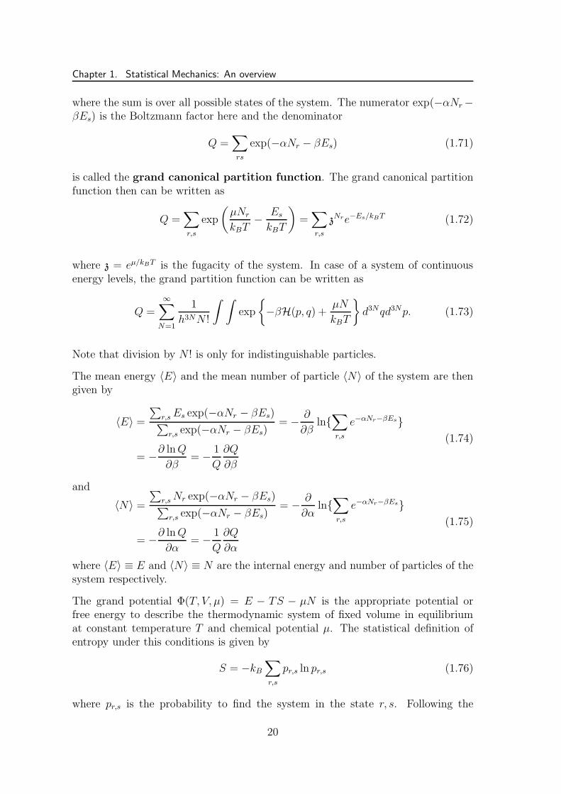
Figure 1.2: Plot of mean occupation number 〈ns〉 of a single-particle energy state εs ina system of non-interacting particles: curve 1 is for fermions, curve 2 for bosons and curve3 for the particles obeying Maxwell-Boltzmann statistics.

This is the Bose-Einstein (BE) distribution where always µ < εs, otherwise 〈ns〉could be negative.

FD Statistics: The fermions have only two states, ns = 0 or 1. Thus, the grandcanonical partition function for N indistinguishable fermions is given by

lnQ =∑

s

ln(

1 + e−β(εs−µ))

(1.112)

The number of particles is given by

N =1

β

∂ lnQ

∂µ=∑

s

e−β(εs−µ)

1 + e−β(εs−µ)=∑

s

〈ns〉 (1.113)

Thus the average number of molecules in the s level is

〈ns〉FD =1

eβ(εs−µ) + 1. (1.114)

This is the Fermi-Dirac (FD) Distribution. However, in the classical limit T → ∞and ρ→ 0,BE and FD statistics lead to the classical MB statistics.

28

statistical mechanics: an overvie · chapter 1 statistical mechanics: an overview 1.1 introduction...

Documents