statistical inference: clt, confidence intervals, p-values
TRANSCRIPT
Statistical inference: CLT, confidence intervals, p-values
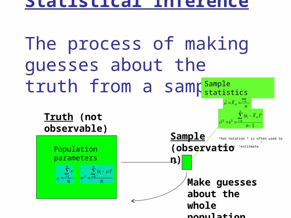
Statistical Inference The process of making guesses about the truth from a sample.
Sample (observation)
Make guesses about the whole population
Truth (not observable)
N
xN
ii
2
12
)(
N
xN
i 1
Population parameters
1
)(
ˆ
2
122
n
Xx
sn
n
ii
n
x
X
n
in
1̂
Sample statistics
*hat notation ^ is often used to indicate
“estitmate”
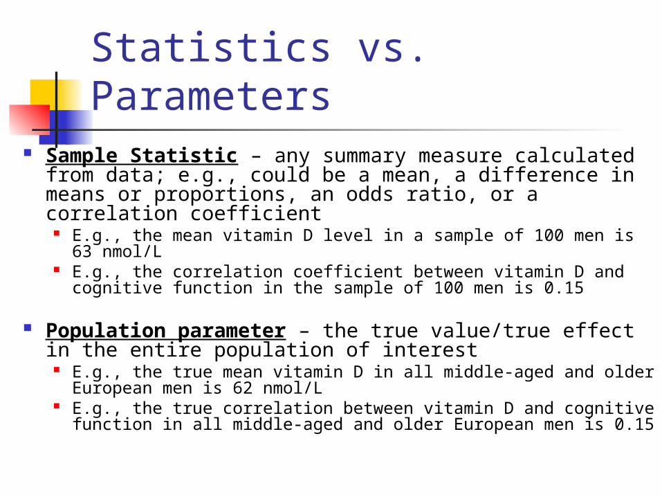
Statistics vs. Parameters Sample Statistic – any summary measure calculated
from data; e.g., could be a mean, a difference in means or proportions, an odds ratio, or a correlation coefficient
E.g., the mean vitamin D level in a sample of 100 men is 63 nmol/L
E.g., the correlation coefficient between vitamin D and cognitive function in the sample of 100 men is 0.15
Population parameter – the true value/true effect in the entire population of interest
E.g., the true mean vitamin D in all middle-aged and older European men is 62 nmol/L
E.g., the true correlation between vitamin D and cognitive function in all middle-aged and older European men is 0.15
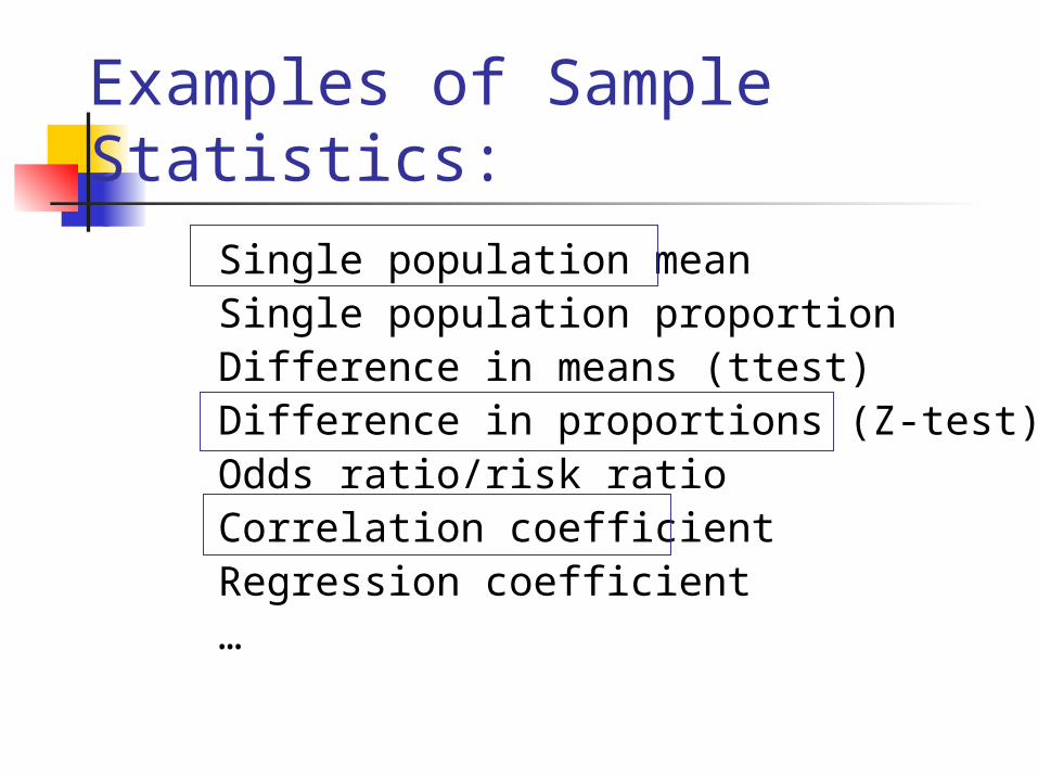
Examples of Sample Statistics:
Single population mean Single population proportionDifference in means (ttest)Difference in proportions (Z-test)Odds ratio/risk ratioCorrelation coefficientRegression coefficient…
Example 1: cognitive function and vitamin D Hypothetical data loosely based on [1]; cross-
sectional study of 100 middle-aged and older European men.
Estimation: What is the average serum vitamin D in middle-aged and older European men?
Sample statistic: mean vitamin D levels Hypothesis testing: Are vitamin D levels and
cognitive function correlated? Sample statistic: correlation coefficient between
vitamin D and cognitive function, measured by the Digit Symbol Substitution Test (DSST).
1. Lee DM, Tajar A, Ulubaev A, et al. Association between 25-hydroxyvitamin D levels and cognitive performance in middle-aged and older European men. J Neurol Neurosurg Psychiatry. 2009 Jul;80(7):722-9.
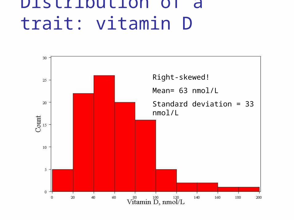
Distribution of a trait: vitamin D
Right-skewed!
Mean= 63 nmol/L
Standard deviation = 33 nmol/L
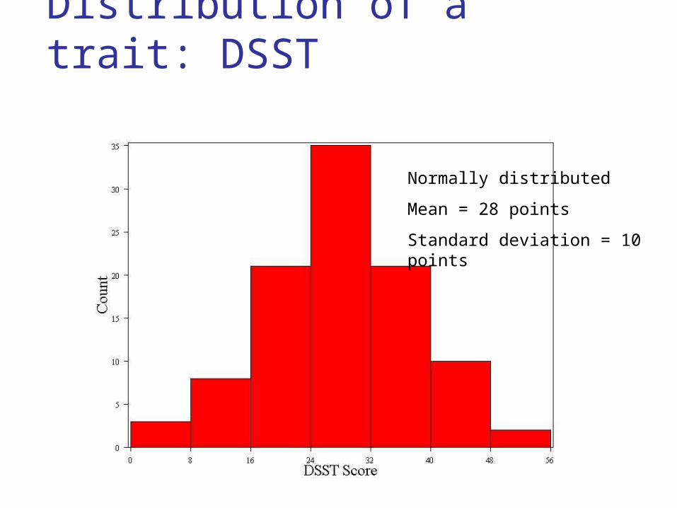
Distribution of a trait: DSST
Normally distributed
Mean = 28 points
Standard deviation = 10 points
Distribution of a statistic… Statistics follow distributions too… But the distribution of a statistic is a
theoretical construct. Statisticians ask a thought experiment: how
much would the value of the statistic fluctuate if one could repeat a particular study over and over again with different samples of the same size?
By answering this question, statisticians are able to pinpoint exactly how much uncertainty is associated with a given statistic.
Distribution of a statistic Two approaches to determine the
distribution of a statistic: 1. Computer simulation
Repeat the experiment over and over again virtually!
More intuitive; can directly observe the behavior of statistics.
2. Mathematical theory Proofs and formulas! More practical; use formulas to solve problems.
Example of computer simulation…
How many heads come up in 100 coin tosses?
Flip coins virtually Flip a coin 100 times; count the number
of heads. Repeat this over and over again a large
number of times (we’ll try 30,000 repeats!)
Plot the 30,000 results.
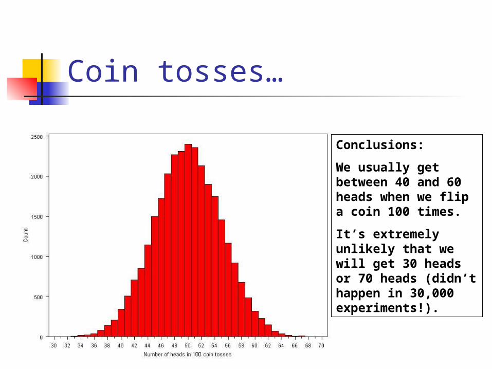
Coin tosses…
Conclusions:
We usually get between 40 and 60 heads when we flip a coin 100 times.
It’s extremely unlikely that we will get 30 heads or 70 heads (didn’t happen in 30,000 experiments!).
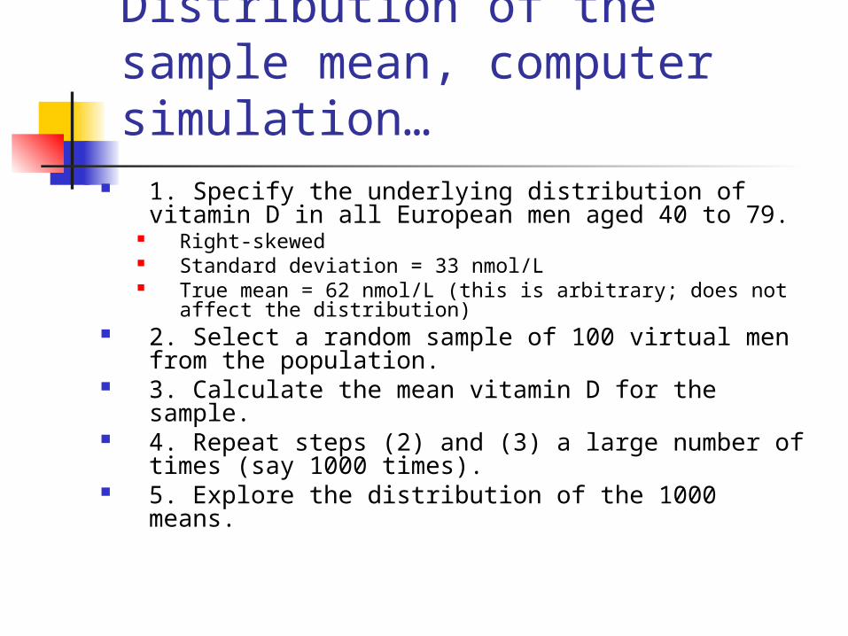
Distribution of the sample mean, computer simulation…
1. Specify the underlying distribution of vitamin D in all European men aged 40 to 79.
Right-skewed Standard deviation = 33 nmol/L True mean = 62 nmol/L (this is arbitrary; does not
affect the distribution) 2. Select a random sample of 100 virtual men
from the population. 3. Calculate the mean vitamin D for the
sample. 4. Repeat steps (2) and (3) a large number of
times (say 1000 times). 5. Explore the distribution of the 1000 means.
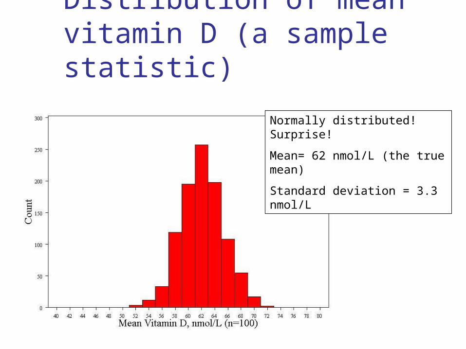
Distribution of mean vitamin D (a sample statistic)
Normally distributed! Surprise!
Mean= 62 nmol/L (the true mean)
Standard deviation = 3.3 nmol/L

Normally distributed (even though the trait is right-skewed!)
Mean = true mean Standard deviation = 3.3 nmol/L
The standard deviation of a statistic is called a standard error
The standard error of a mean =
Distribution of mean vitamin D (a sample statistic)
n
s
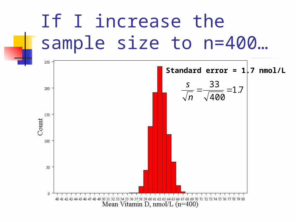
If I increase the sample size to n=400…
Standard error = 1.7 nmol/L
7.1400
33
n
s
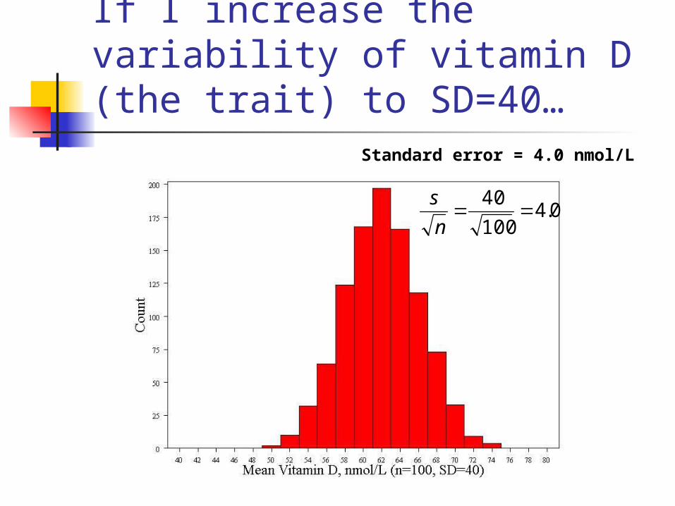
If I increase the variability of vitamin D (the trait) to SD=40…
Standard error = 4.0 nmol/L
0.4100
40
n
s
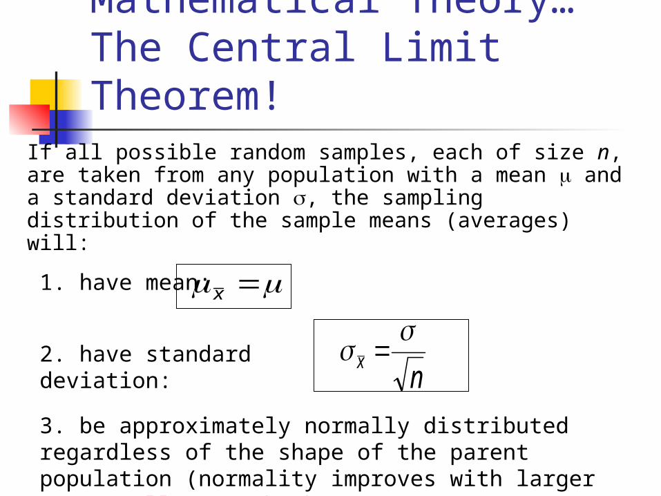
Mathematical Theory…The Central Limit Theorem!
If all possible random samples, each of size n, are taken from any population with a mean and a standard deviation , the sampling distribution of the sample means (averages) will:
x1. have mean:
nx
2. have standard deviation:
3. be approximately normally distributed regardless of the shape of the parent population (normality improves with larger n). It all comes back to Z!
Symbol Check
x The mean of the sample means.
x The standard deviation of the sample means. Also called “the standard error of the mean.”
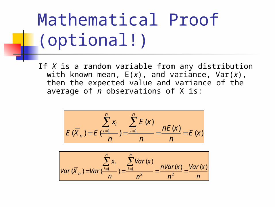
Mathematical Proof (optional!)If X is a random variable from any distribution with known
mean, E(x), and variance, Var(x), then the expected value and variance of the average of n observations of X is:
)()(
)(
)()( 11 xEn
xnE
n
xE
n
x
EXE
n
i
n
ii
n
n
xVar
n
xnVar
n
xVar
n
x
VarXVar
n
i
n
ii
n
)()()(
)()(22
11
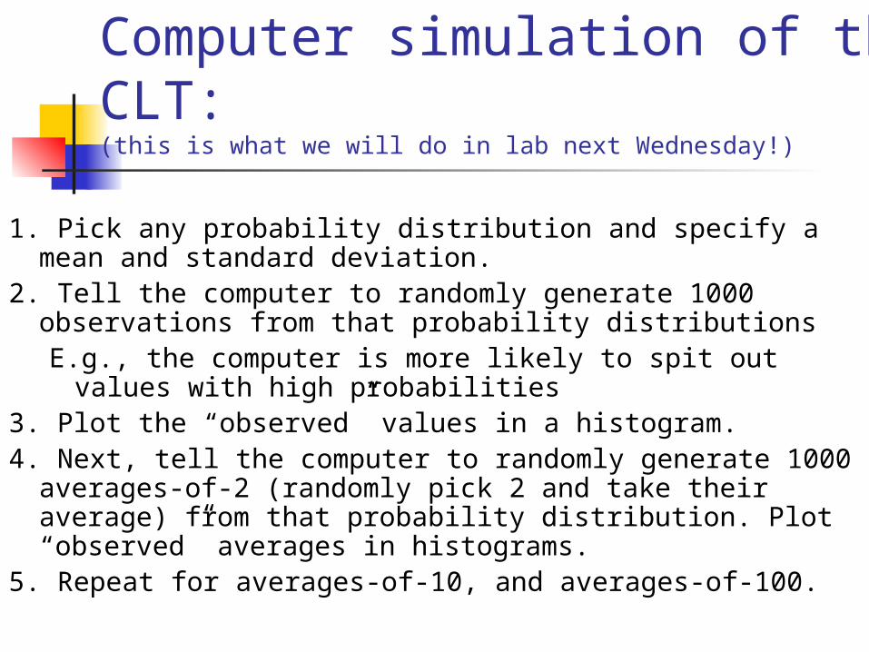
Computer simulation of the CLT:(this is what we will do in lab next Wednesday!)
1. Pick any probability distribution and specify a mean and standard deviation.
2. Tell the computer to randomly generate 1000 observations from that probability distributionsE.g., the computer is more likely to spit out values with
high probabilities3. Plot the “observed” values in a histogram.4. Next, tell the computer to randomly generate 1000
averages-of-2 (randomly pick 2 and take their average) from that probability distribution. Plot “observed” averages in histograms.
5. Repeat for averages-of-10, and averages-of-100.
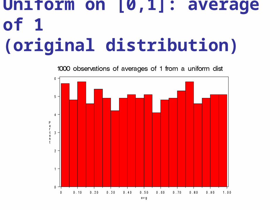
Uniform on [0,1]: average of 1(original distribution)
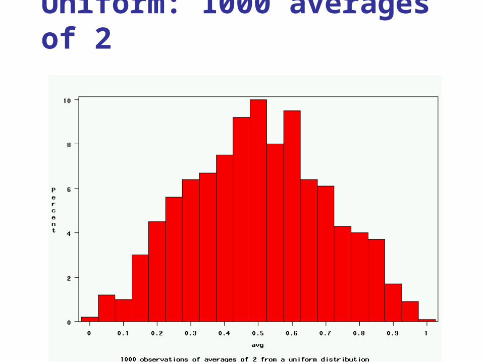
Uniform: 1000 averages of 2
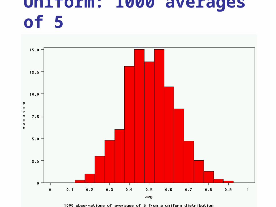
Uniform: 1000 averages of 5
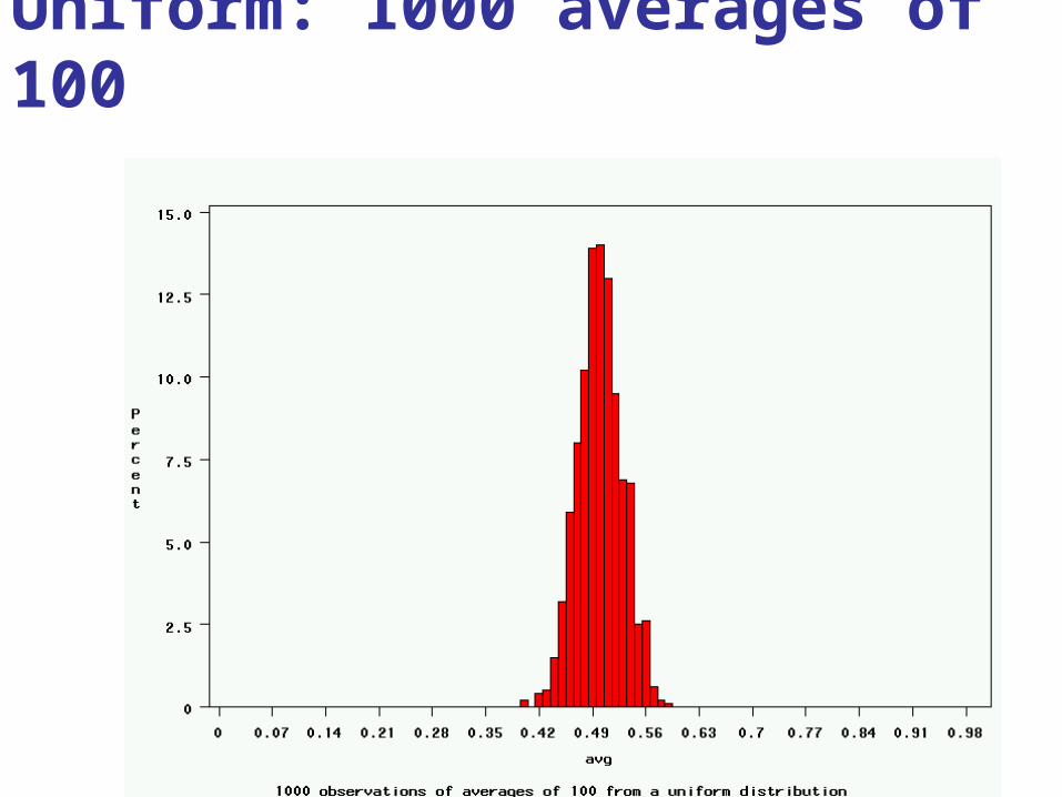
Uniform: 1000 averages of 100
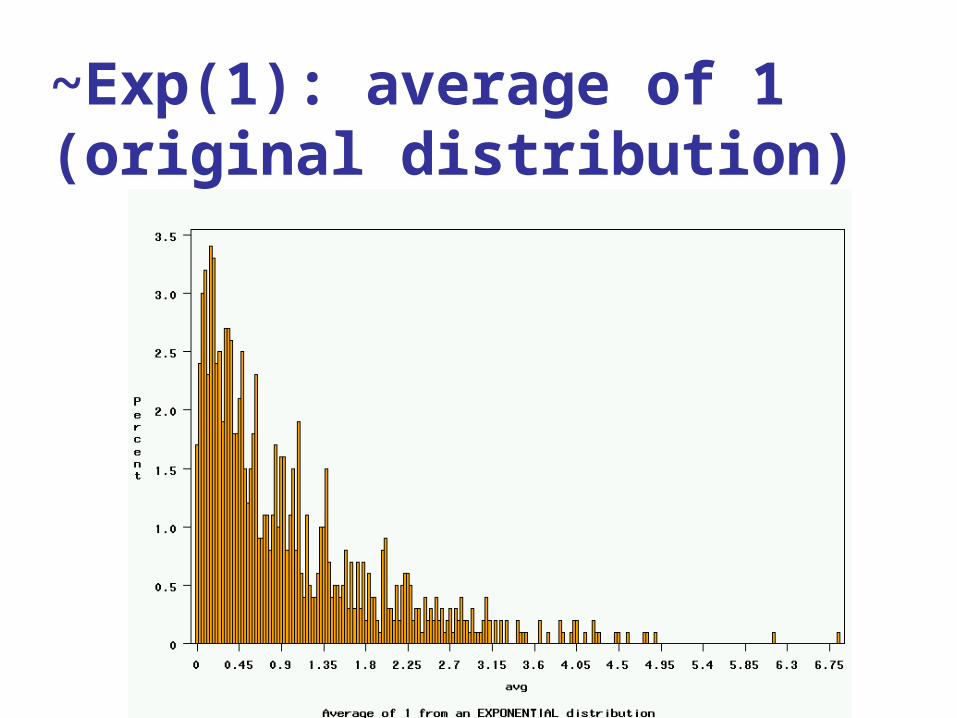
~Exp(1): average of 1(original distribution)
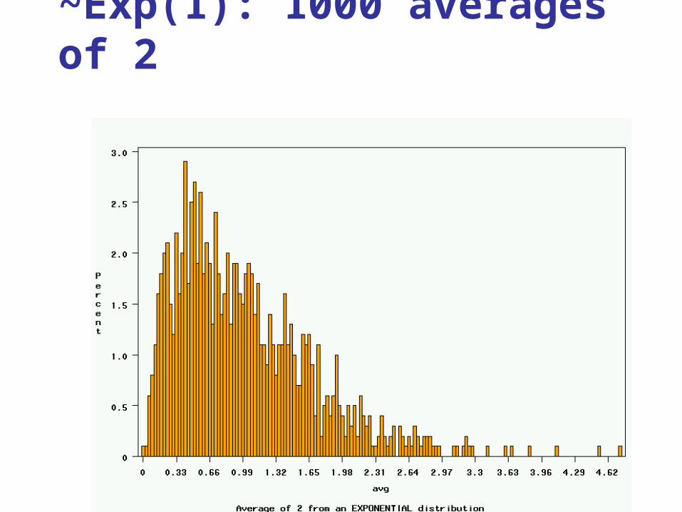
~Exp(1): 1000 averages of 2
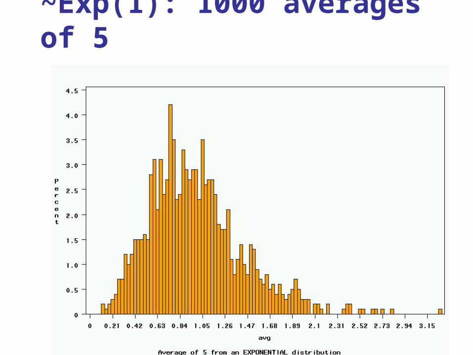
~Exp(1): 1000 averages of 5
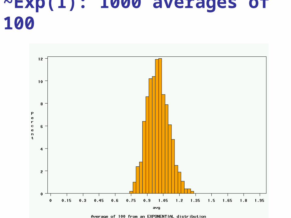
~Exp(1): 1000 averages of 100
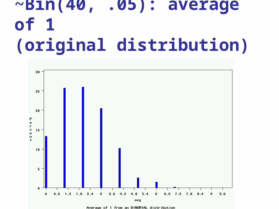
~Bin(40, .05): average of 1(original distribution)
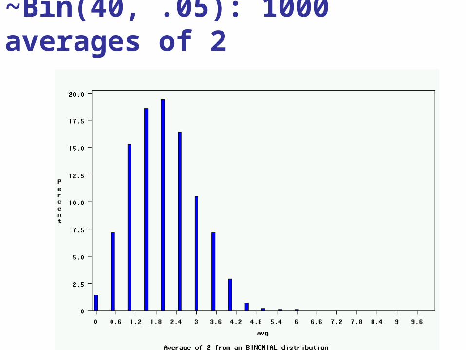
~Bin(40, .05): 1000 averages of 2
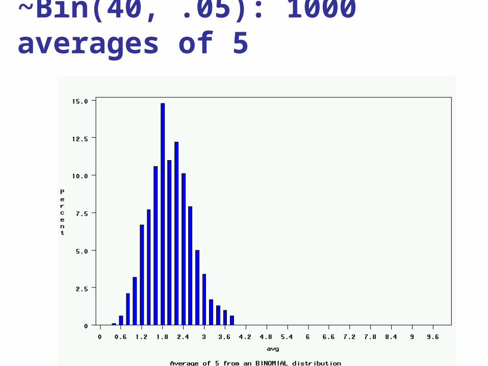
~Bin(40, .05): 1000 averages of 5
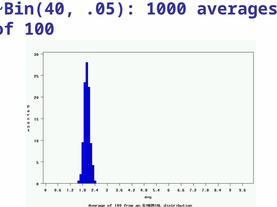
~Bin(40, .05): 1000 averages of 100
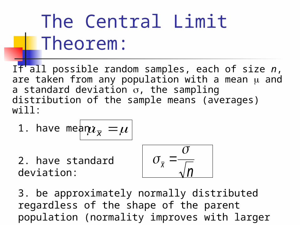
The Central Limit Theorem:
If all possible random samples, each of size n, are taken from any population with a mean and a standard deviation , the sampling distribution of the sample means (averages) will:
x1. have mean:
nx
2. have standard deviation:
3. be approximately normally distributed regardless of the shape of the parent population (normality improves with larger n)
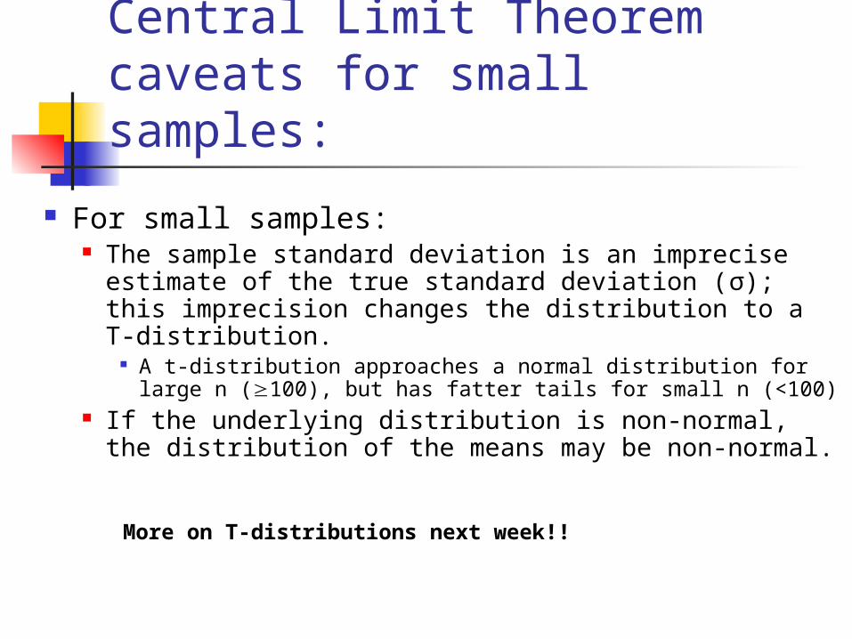
Central Limit Theorem caveats for small samples:
For small samples: The sample standard deviation is an imprecise
estimate of the true standard deviation (σ); this imprecision changes the distribution to a T-distribution.
A t-distribution approaches a normal distribution for large n (100), but has fatter tails for small n (<100)
If the underlying distribution is non-normal, the distribution of the means may be non-normal.
More on T-distributions next week!!
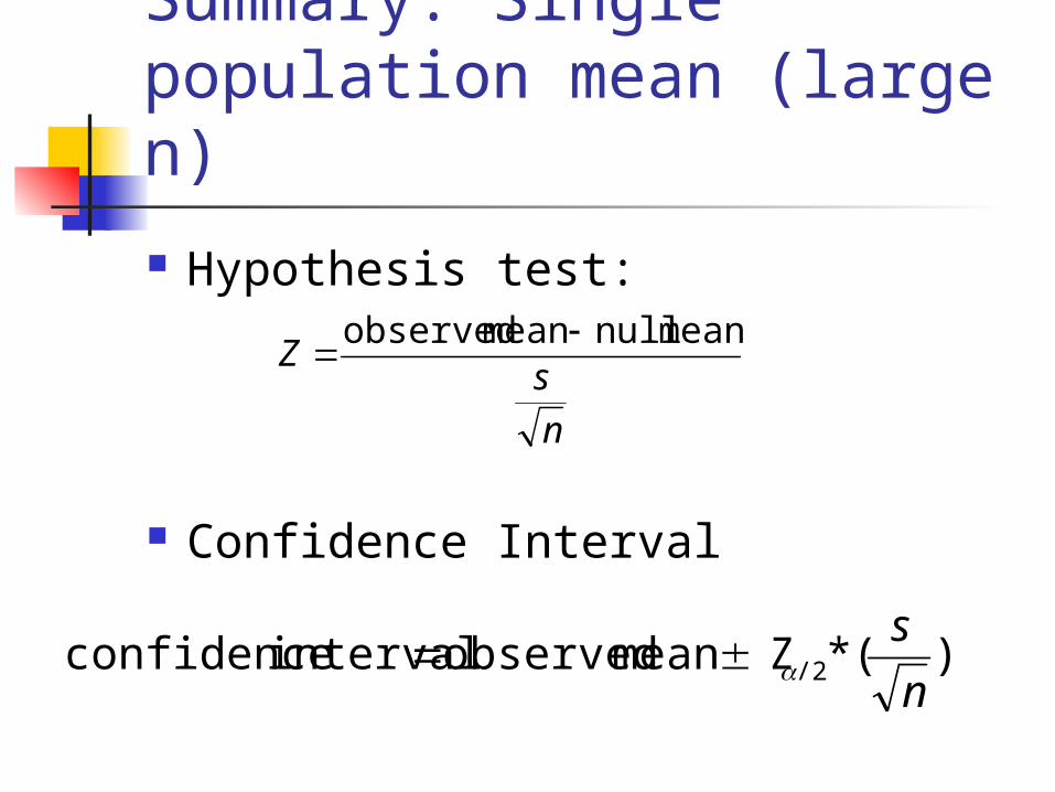
Summary: Single population mean (large n)
Hypothesis test:
Confidence Interval
n
sZ
mean nullmean observed
)(* Zmean observed interval confidence /2n
s
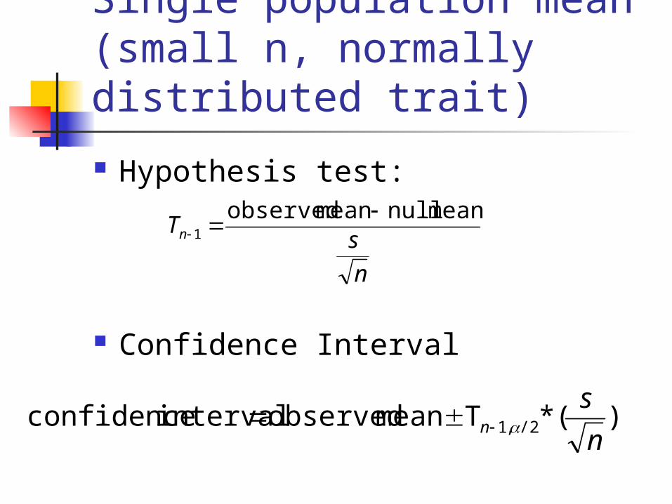
Single population mean (small n, normally distributed trait)
Hypothesis test:
Confidence Interval
n
sTn
mean nullmean observed1
)(*T mean observed interval confidence /2,1n
sn
Examples of Sample Statistics:
Single population mean Single population proportionDifference in means (ttest)Difference in proportions (Z-test)Odds ratio/risk ratioCorrelation coefficientRegression coefficient…
1. Specify the true correlation coefficient Correlation coefficient = 0.15
2. Select a random sample of 100 virtual men from the population.
3. Calculate the correlation coefficient for the sample.
4. Repeat steps (2) and (3) 15,000 times 5. Explore the distribution of the 15,000
correlation coefficients.
Distribution of a correlation coefficient?? Computer simulation…
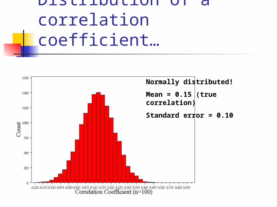
Distribution of a correlation coefficient…
Normally distributed!
Mean = 0.15 (true correlation)
Standard error = 0.10
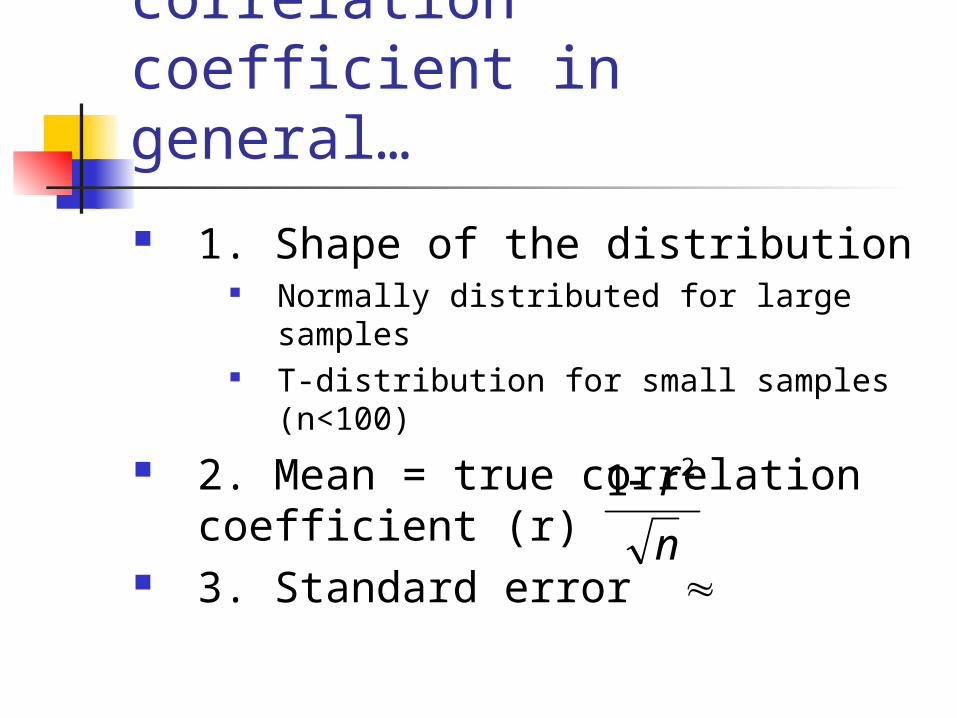
Distribution of a correlation coefficient in general…
1. Shape of the distribution Normally distributed for large samples T-distribution for small samples (n<100)
2. Mean = true correlation coefficient (r)
3. Standard error n
r 21
Many statistics follow normal (or t-distributions)…
Means/difference in means T-distribution for small samples
Proportions/difference in proportions
Regression coefficients T-distribution for small samples
Natural log of the odds ratio
Estimation (confidence intervals)…
What is a good estimate for the true mean vitamin D in the population (the population parameter)? 63 nmol/L +/- margin of error
95% confidence interval Goal: capture the true effect (e.g.,
the true mean) most of the time. A 95% confidence interval should
include the true effect about 95% of the time.
A 99% confidence interval should include the true effect about 99% of the time.
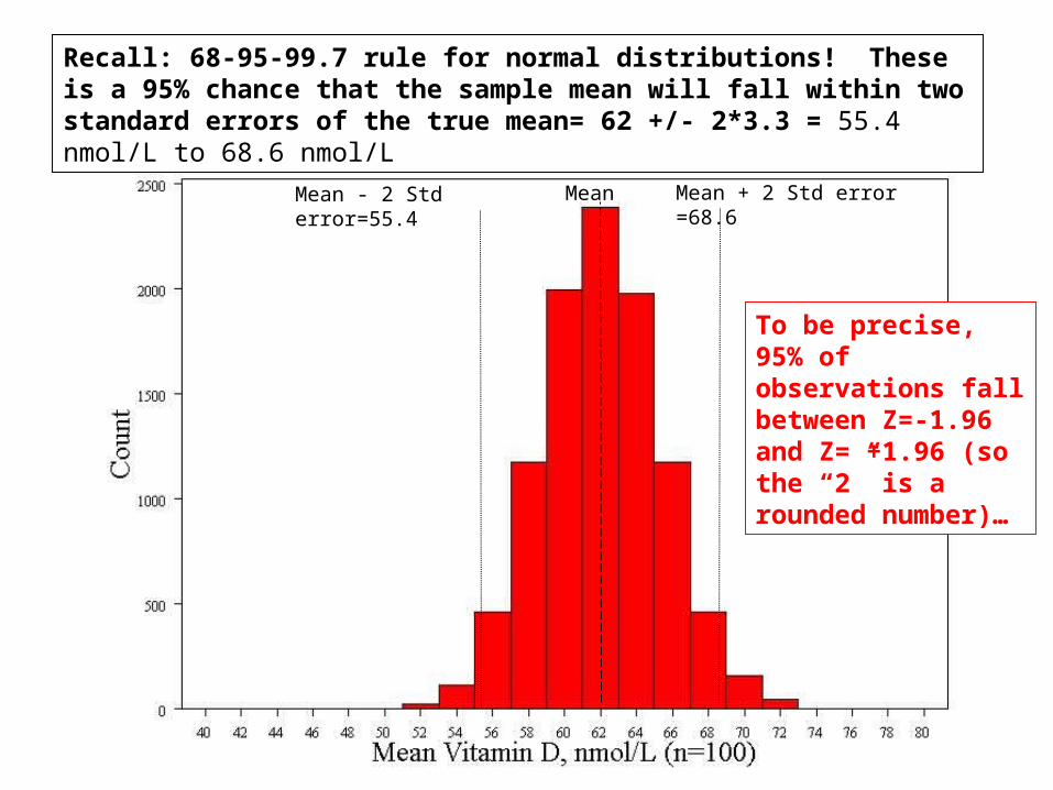
Mean Mean + 2 Std error =68.6Mean - 2 Std error=55.4
Recall: 68-95-99.7 rule for normal distributions! These is a 95% chance that the sample mean will fall within two standard errors of the true mean= 62 +/- 2*3.3 = 55.4 nmol/L to 68.6 nmol/L
To be precise, 95% of observations fall between Z=-1.96 and Z= +1.96 (so the “2” is a rounded number)…
95% confidence interval There is a 95% chance that the sample
mean is between 55.4 nmol/L and 68.6 nmol/L
For every sample mean in this range, sample mean +/- 2 standard errors will include the true mean: For example, if the sample mean is 68.6
nmol/L: 95% CI = 68.6 +/- 6.6 = 62.0 to 75.2 This interval just hits the true mean, 62.0.
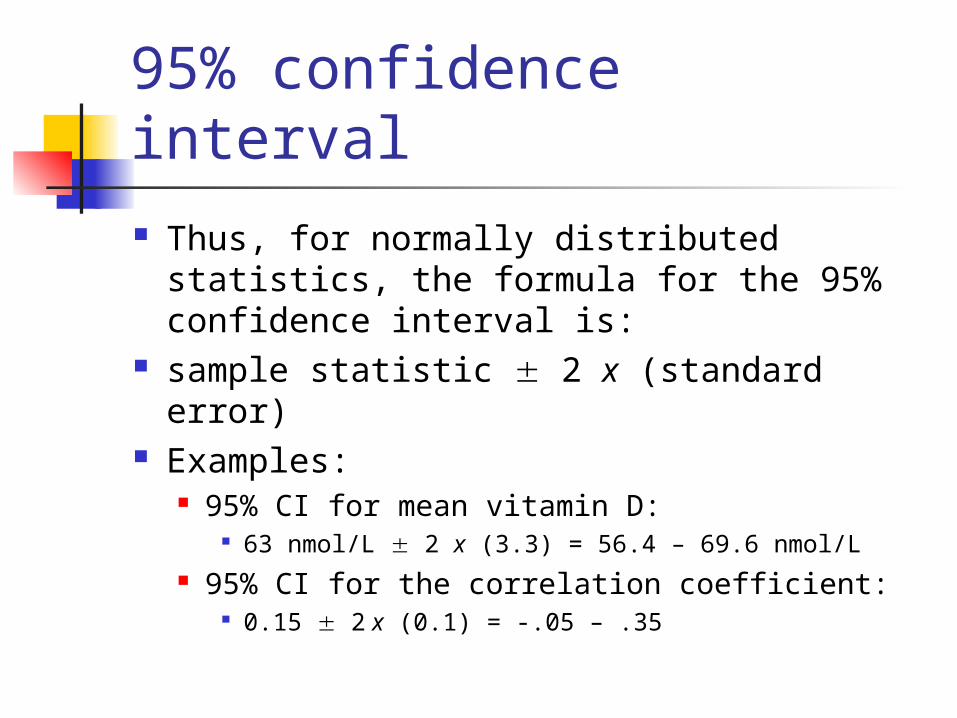
95% confidence interval Thus, for normally distributed statistics,
the formula for the 95% confidence interval is:
sample statistic 2 x (standard error) Examples:
95% CI for mean vitamin D: 63 nmol/L 2 x (3.3) = 56.4 – 69.6 nmol/L
95% CI for the correlation coefficient: 0.15 2 x (0.1) = -.05 – .35
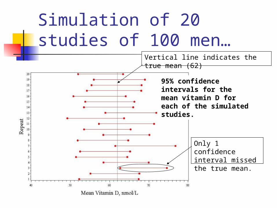
Simulation of 20 studies of 100 men…
95% confidence intervals for the mean vitamin D for each of the simulated studies.
Only 1 confidence interval missed the true mean.
Vertical line indicates the true mean (62)
Confidence Intervals give:*A plausible range of values for a population parameter.
*The precision of an estimate.(When sampling variability is high, the confidence interval will be wide to reflect the uncertainty of the observation.)
*Statistical significance (if the 95% CI does not cross the null value, it is significant at .05)
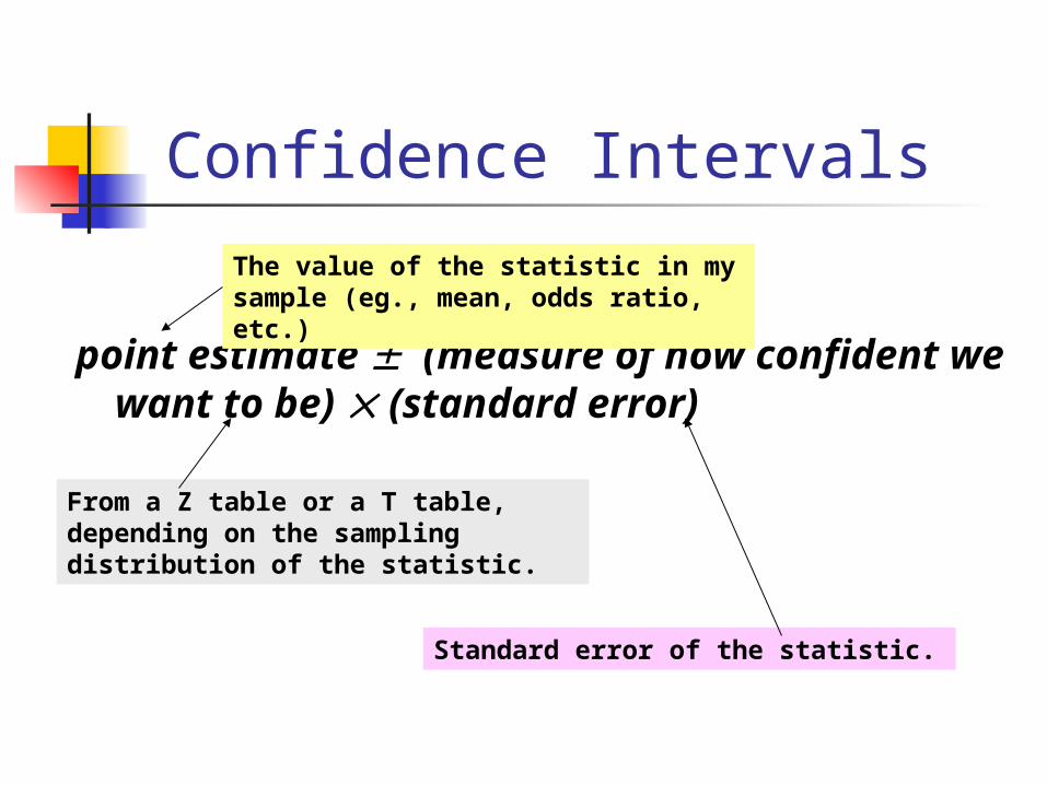
Confidence Intervals
point estimate (measure of how confident we want to be) (standard error)
The value of the statistic in my sample (eg., mean, odds ratio, etc.)
From a Z table or a T table, depending on the sampling distribution of the statistic.
Standard error of the statistic.
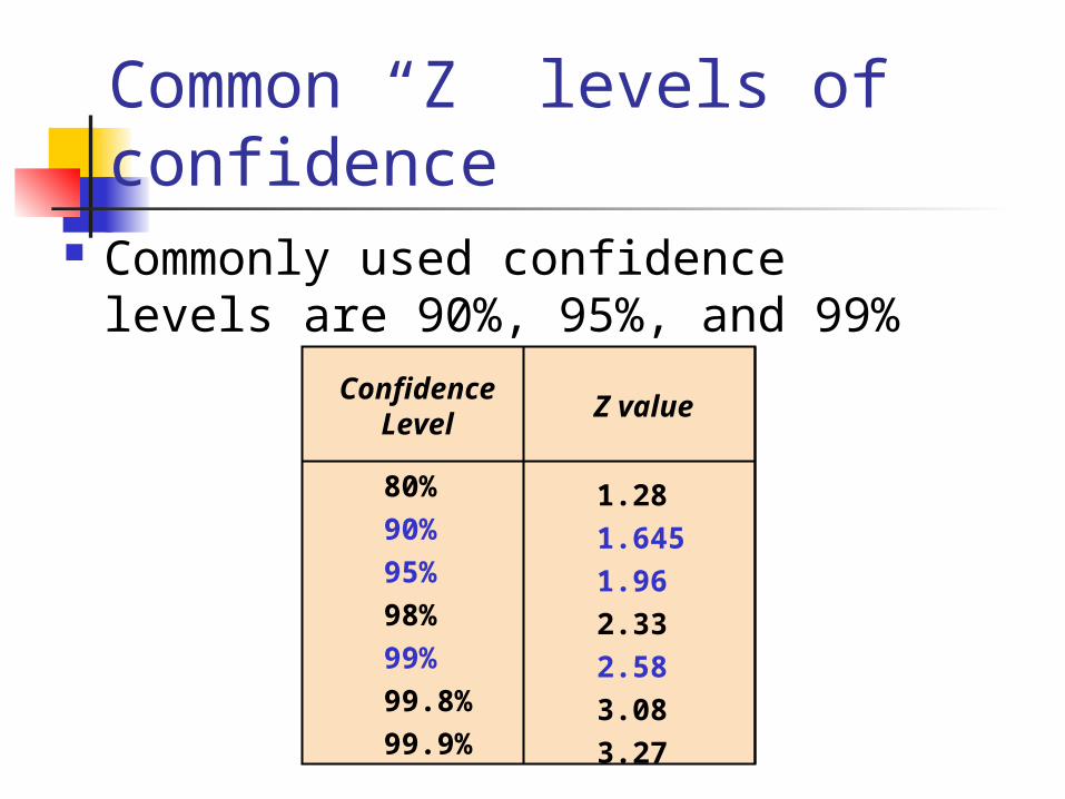
Common “Z” levels of confidence
Commonly used confidence levels are 90%, 95%, and 99%
Confidence Level
Z value
1.28
1.645
1.96
2.33
2.58
3.08
3.27
80%
90%
95%
98%
99%
99.8%
99.9%
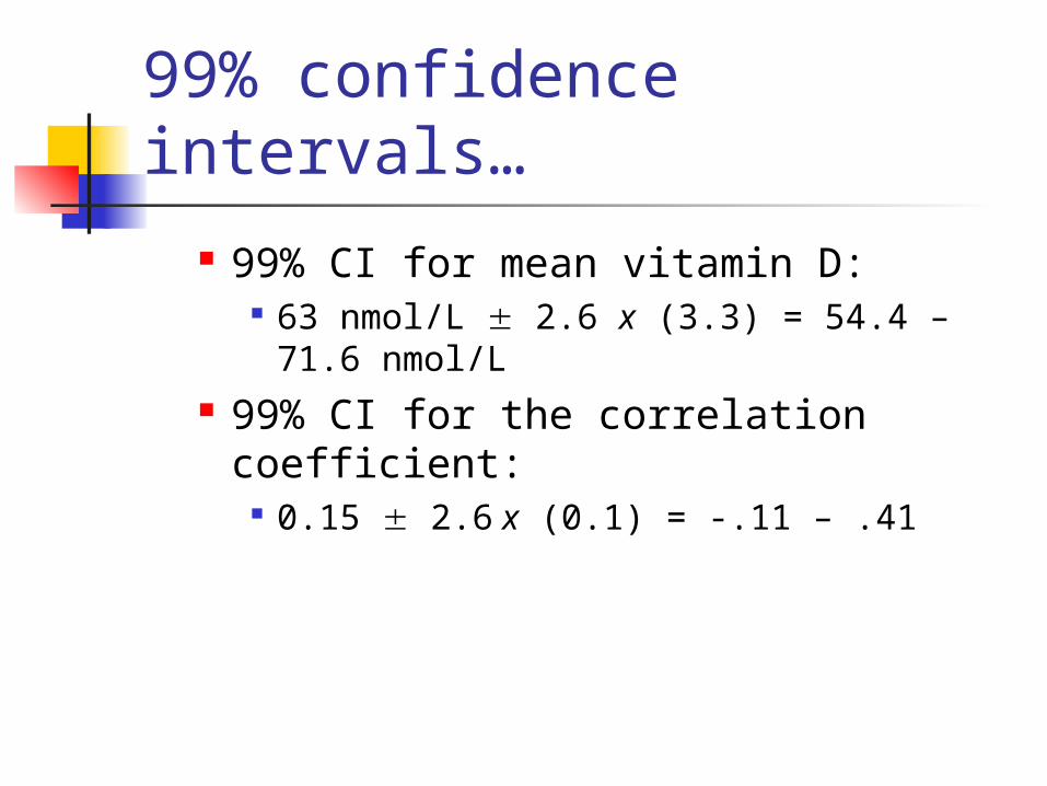
99% confidence intervals…
99% CI for mean vitamin D: 63 nmol/L 2.6 x (3.3) = 54.4 – 71.6
nmol/L 99% CI for the correlation coefficient:
0.15 2.6 x (0.1) = -.11 – .41
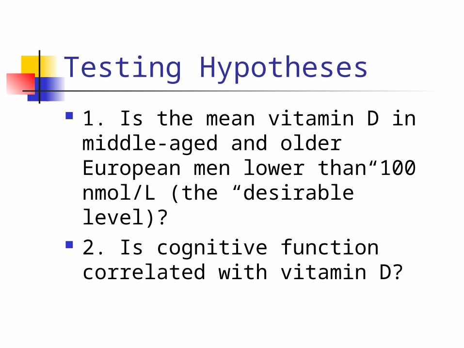
Testing Hypotheses
1. Is the mean vitamin D in middle-aged and older European men lower than 100 nmol/L (the “desirable” level)?
2. Is cognitive function correlated with vitamin D?
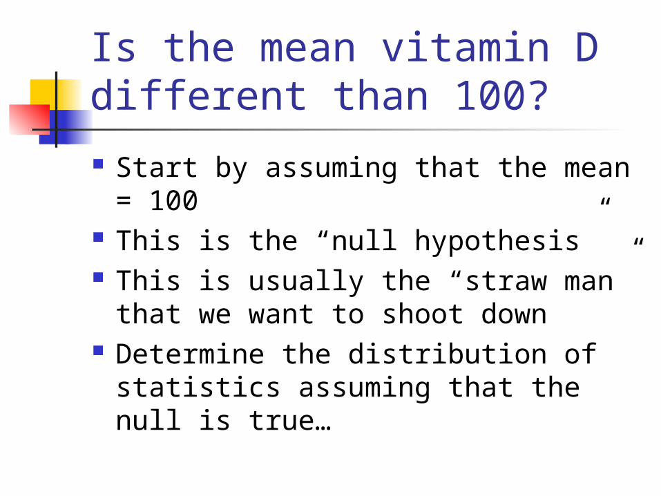
Is the mean vitamin D different than 100?
Start by assuming that the mean = 100
This is the “null hypothesis” This is usually the “straw man” that
we want to shoot down Determine the distribution of
statistics assuming that the null is true…
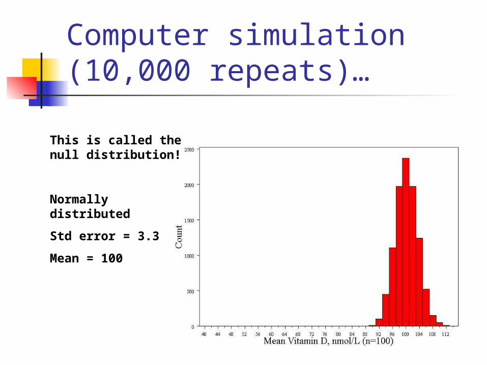
Computer simulation (10,000 repeats)…
This is called the null distribution!
Normally distributed
Std error = 3.3
Mean = 100
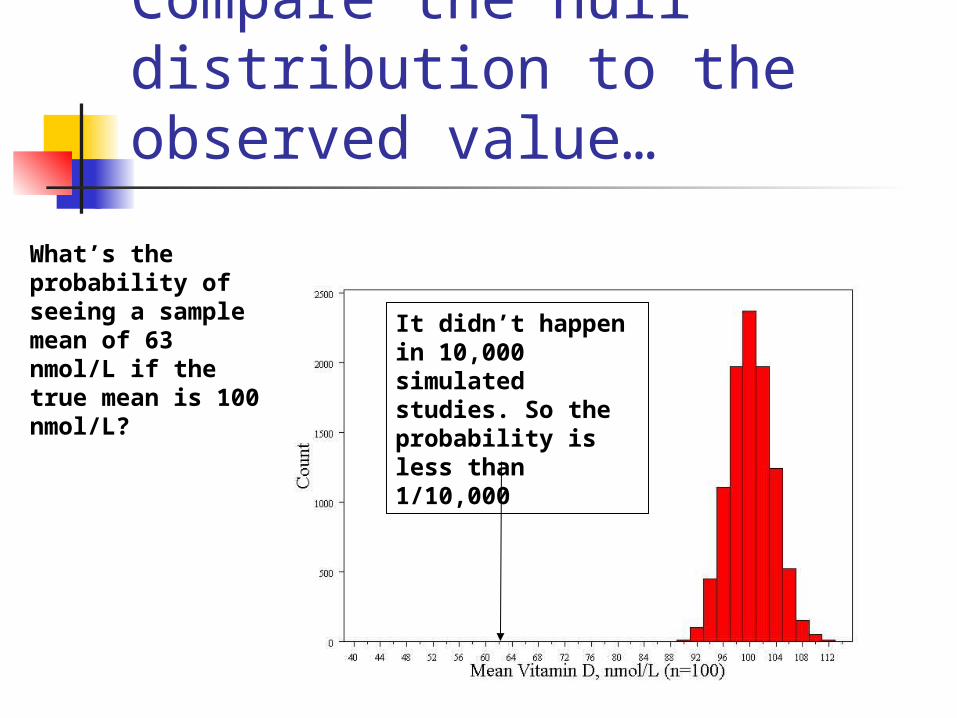
Compare the null distribution to the observed value…
What’s the probability of seeing a sample mean of 63 nmol/L if the true mean is 100 nmol/L?
It didn’t happen in 10,000 simulated studies. So the probability is less than 1/10,000
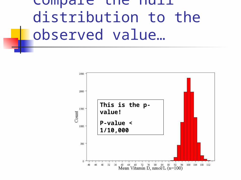
Compare the null distribution to the observed value…
This is the p-value!
P-value < 1/10,000
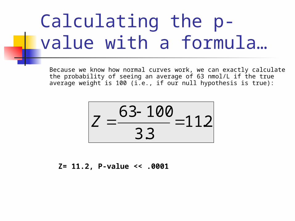
Calculating the p-value with a formula…
Because we know how normal curves work, we can exactly calculate the probability of seeing an average of 63 nmol/L if the true average weight is 100 (i.e., if our null hypothesis is true):
2.113.3
10063
Z
Z= 11.2, P-value << .0001
The P-valueP-value is the probability that we would have seen our data (or something more unexpected) just by chance if the null hypothesis (null value) is true.
Small p-values mean the null value is unlikely given our data.
Our data are so unlikely given the null hypothesis (<<1/10,000) that I’m going to reject the null hypothesis! (Don’t want to reject our data!)
P-value<.0001 means:
The probability of seeing what you saw or something more extreme if the null hypothesis is true (due to chance)<.0001
P(empirical data/null hypothesis) <.0001
The P-value By convention, p-values of <.05 are
often accepted as “statistically significant” in the medical literature; but this is an arbitrary cut-off.
A cut-off of p<.05 means that in about 5 of 100 experiments, a result would appear significant just by chance (“Type I error”).
Summary: Hypothesis Testing
The Steps:1. Define your hypotheses (null, alternative)2. Specify your null distribution 3. Do an experiment4. Calculate the p-value of what you
observed 5. Reject or fail to reject (~accept) the null
hypothesis
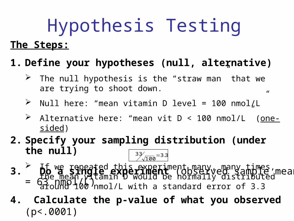
Hypothesis TestingThe Steps:
1. Define your hypotheses (null, alternative)
The null hypothesis is the “straw man” that we are trying to shoot down.
Null here: “mean vitamin D level = 100 nmol/L”
Alternative here: “mean vit D < 100 nmol/L” (one-sided)
2. Specify your sampling distribution (under the null)
If we repeated this experiment many, many times, the mean vitamin D would be normally distributed around 100 nmol/L with a standard error of 3.3 3.3
10033
3. Do a single experiment (observed sample mean = 63 nmol/L)
4. Calculate the p-value of what you observed (p<.0001)
5. Reject or fail to reject the null hypothesis (reject)
Confidence intervals give the same information (and more) than hypothesis tests…
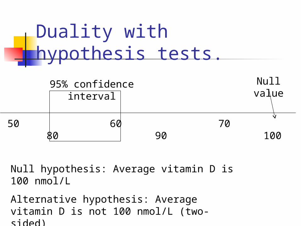
Duality with hypothesis tests.
Null value95% confidence interval
Null hypothesis: Average vitamin D is 100 nmol/L
Alternative hypothesis: Average vitamin D is not 100 nmol/L (two-sided)
P-value < .05
50 60 70 80 90 100
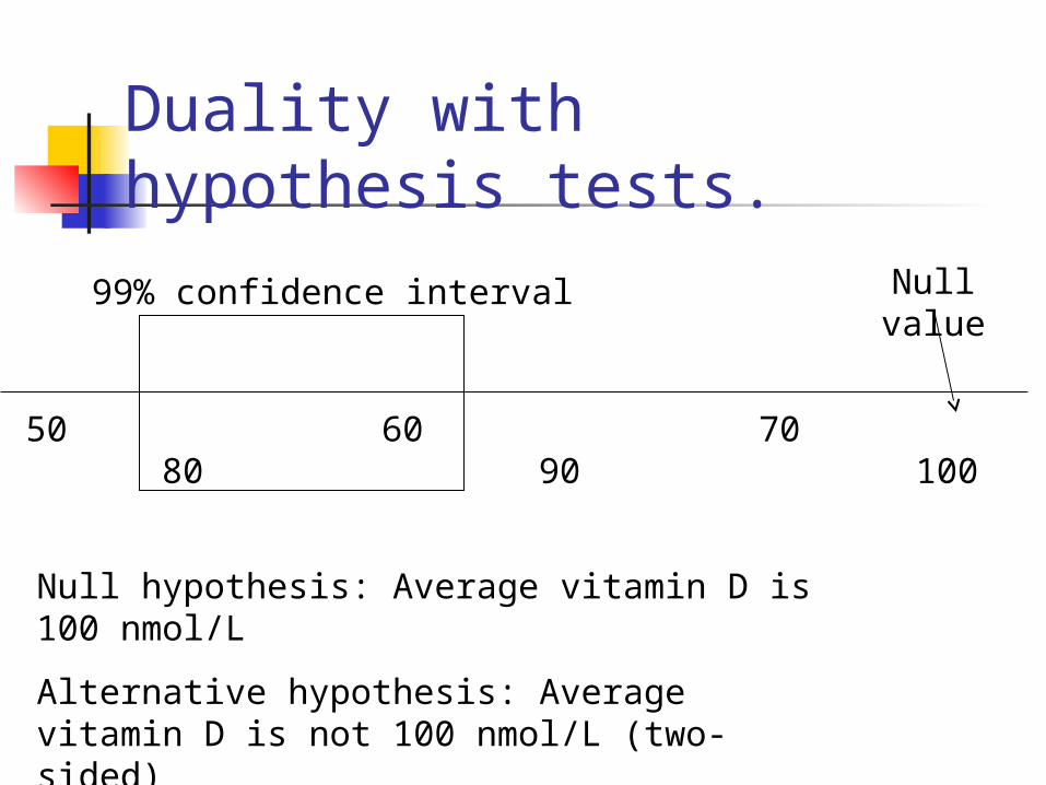
Duality with hypothesis tests.
Null value99% confidence interval
Null hypothesis: Average vitamin D is 100 nmol/L
Alternative hypothesis: Average vitamin D is not 100 nmol/L (two-sided)
P-value < .01
50 60 70 80 90 100
2. Is cognitive function correlated with vitamin D?
Null hypothesis: r = 0 Alternative hypothesis: r 0
Two-sided hypothesis Doesn’t assume that the correlation
will be positive or negative.
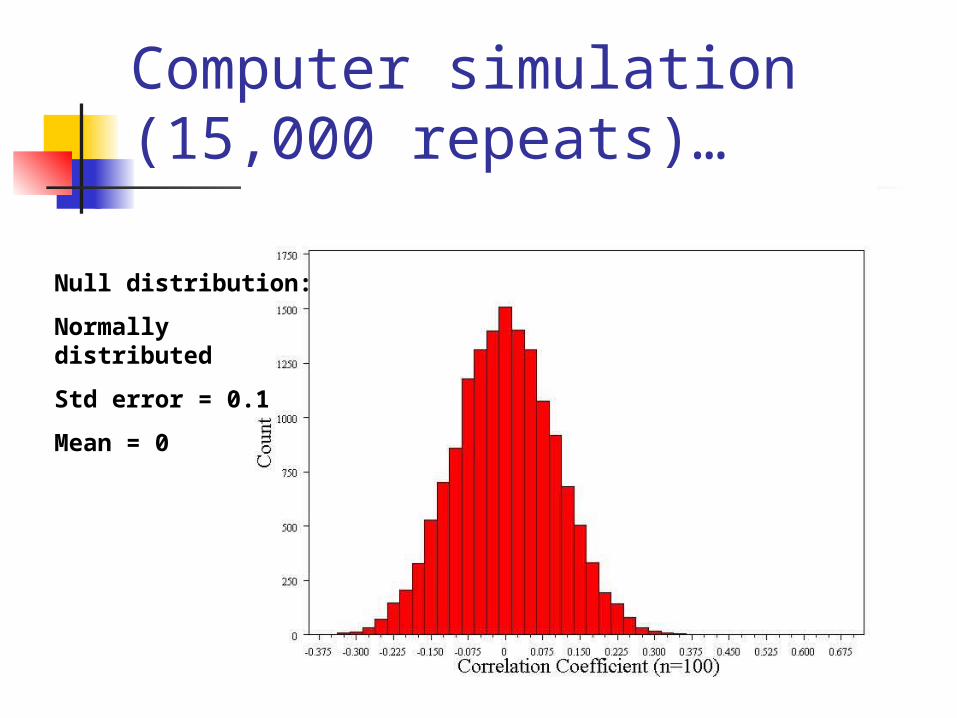
Computer simulation (15,000 repeats)…
Null distribution:
Normally distributed
Std error = 0.1
Mean = 0
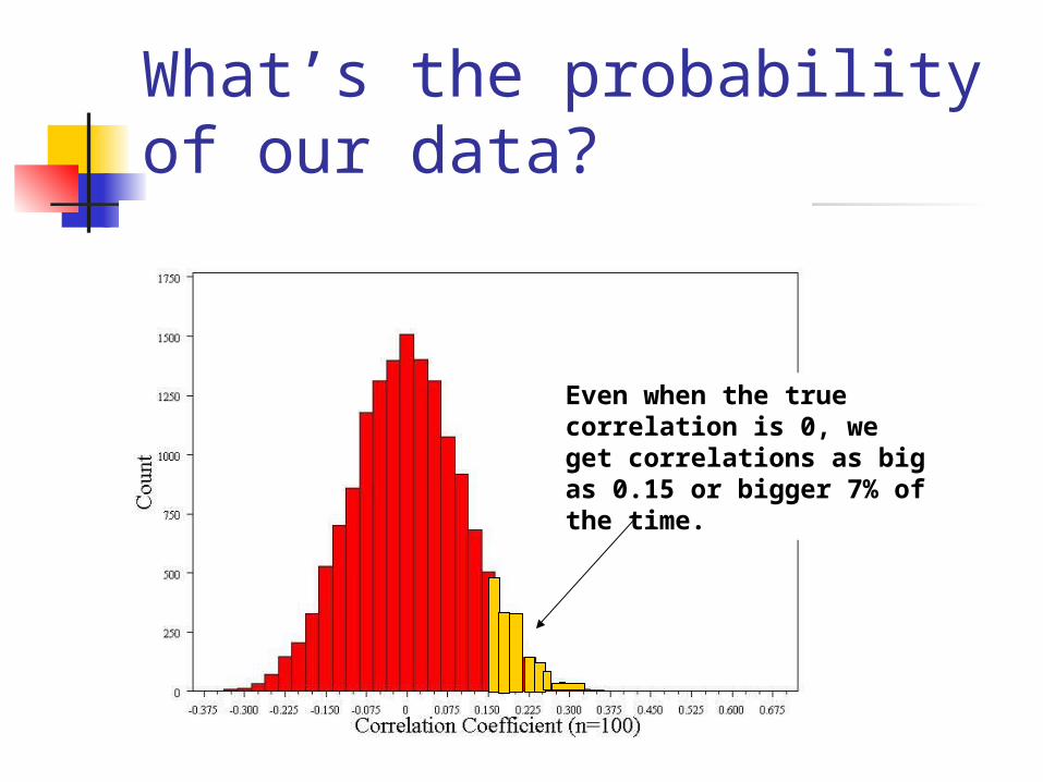
What’s the probability of our data?
Even when the true correlation is 0, we get correlations as big as 0.15 or bigger 7% of the time.
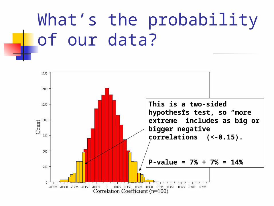
What’s the probability of our data?
This is a two-sided hypothesis test, so “more extreme” includes as big or bigger negative correlations (<-0.15).
P-value = 7% + 7% = 14%
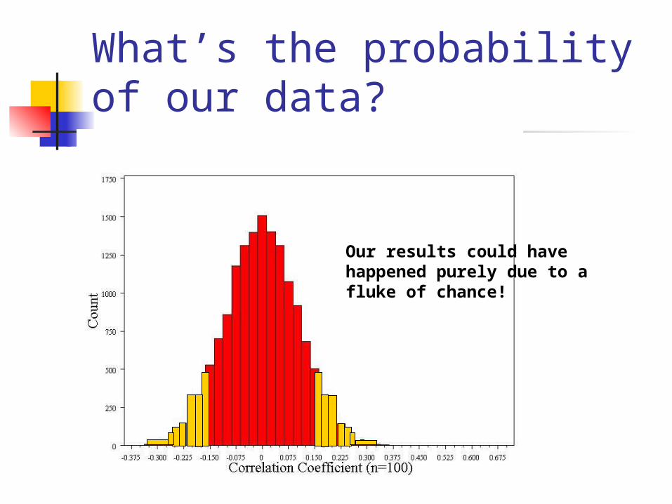
What’s the probability of our data?
Our results could have happened purely due to a fluke of chance!
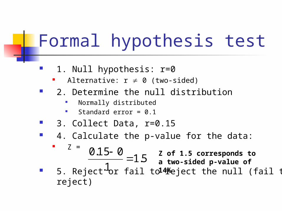
Formal hypothesis test 1. Null hypothesis: r=0
Alternative: r 0 (two-sided) 2. Determine the null distribution
Normally distributed Standard error = 0.1
3. Collect Data, r=0.15 4. Calculate the p-value for the data:
Z =
5. Reject or fail to reject the null (fail to reject)
5.11.
015.0
Z of 1.5 corresponds to a two-sided p-value of 14%
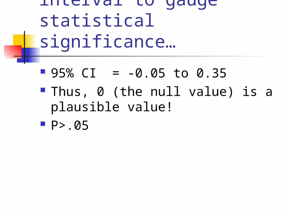
Or use confidence interval to gauge statistical significance…
95% CI = -0.05 to 0.35 Thus, 0 (the null value) is a
plausible value! P>.05

Examples of Sample Statistics:
Single population mean Single population proportionDifference in means (ttest)Difference in proportions (Z-test)Odds ratio/risk ratioCorrelation coefficientRegression coefficient…
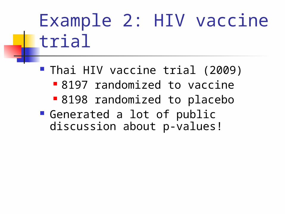
Example 2: HIV vaccine trial Thai HIV vaccine trial (2009)
8197 randomized to vaccine 8198 randomized to placebo
Generated a lot of public discussion about p-values!
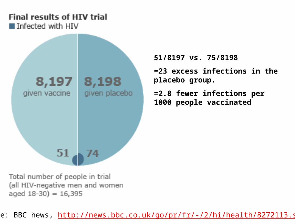
Source: BBC news, http://news.bbc.co.uk/go/pr/fr/-/2/hi/health/8272113.stm
51/8197 vs. 75/8198
=23 excess infections in the placebo group.
=2.8 fewer infections per 1000 people vaccinated
Null hypothesis
Null hypothesis: infection rate is the same in the two groups
Alternative hypothesis: infection rates differ
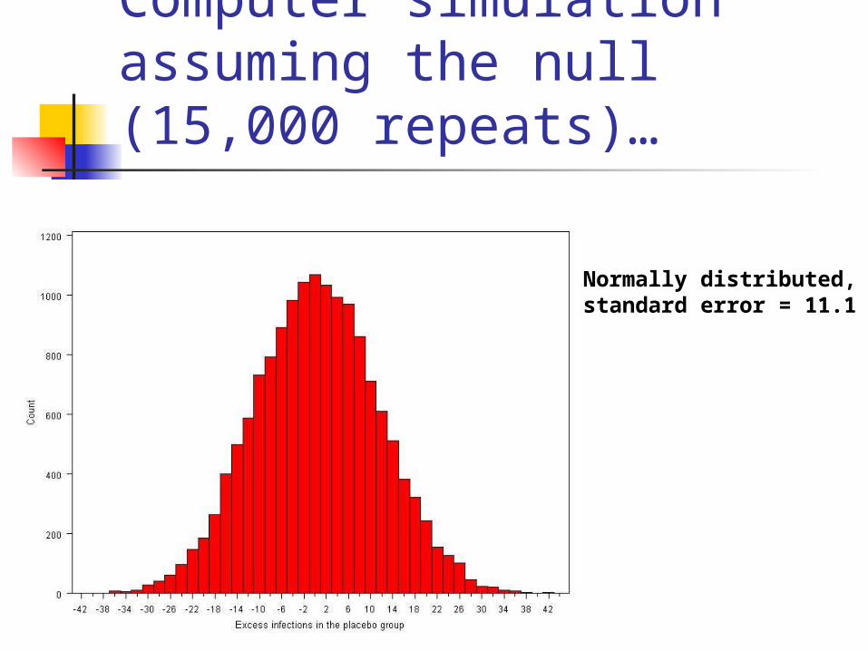
Computer simulation assuming the null (15,000 repeats)…
Normally distributed, standard error = 11.1
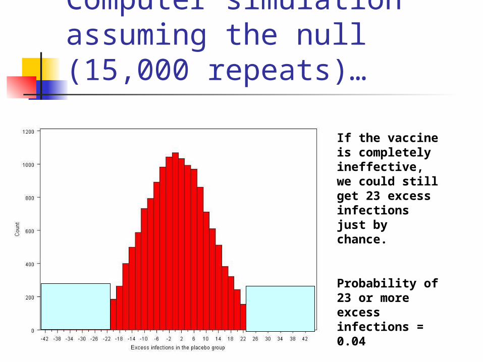
Computer simulation assuming the null (15,000 repeats)…
If the vaccine is completely ineffective, we could still get 23 excess infections just by chance.
Probability of 23 or more excess infections = 0.04
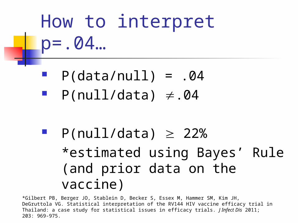
How to interpret p=.04…
P(data/null) = .04 P(null/data) .04
P(null/data) 22%*estimated using Bayes’ Rule (and prior data on the vaccine)
*Gilbert PB, Berger JO, Stablein D, Becker S, Essex M, Hammer SM, Kim JH, DeGruttola VG. Statistical interpretation of the RV144 HIV vaccine efficacy trial in Thailand: a case study for statistical issues in efficacy trials. J Infect Dis 2011; 203: 969-975.
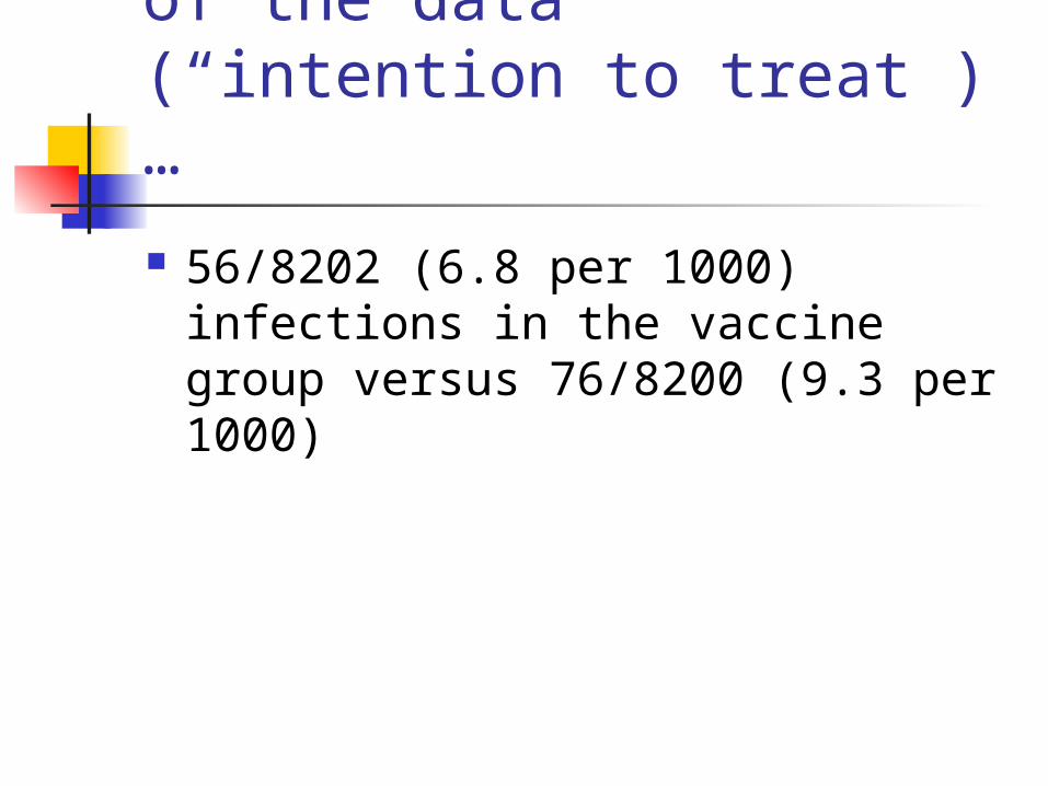
Alternative analysis of the data (“intention to treat”)…
56/8202 (6.8 per 1000) infections in the vaccine group versus 76/8200 (9.3 per 1000)
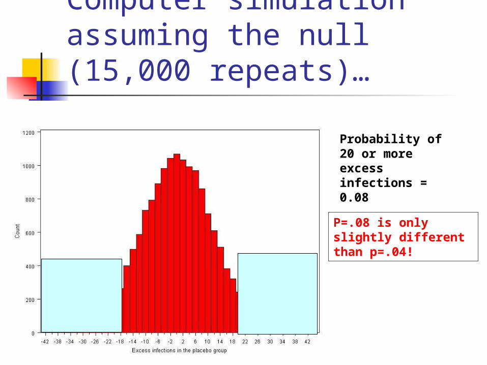
Computer simulation assuming the null (15,000 repeats)…
Probability of 20 or more excess infections = 0.08
P=.08 is only slightly different than p=.04!
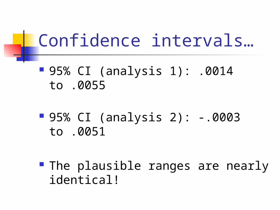
Confidence intervals…
95% CI (analysis 1): .0014 to .0055
95% CI (analysis 2): -.0003 to .0051
The plausible ranges are nearly identical!