State Space Model for the Prediction of EnergyConsumption

Dexiong Chen, Chia-Man Hung

March 1, 2017

Dexiong Chen, Chia-Man Hung 1 / 23

IntroductionMotivation

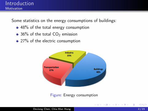
Some statistics on the energy consumptions of buildings:48% of the total energy consumption36% of the total CO2 emission27% of the electric consumption

Figure: Energy consumption

Dexiong Chen, Chia-Man Hung 2 / 23

IntroductionApproaches

Various approaches:physics methodsstatistical methodsneural networks (ANNs)support vector machines (SVMs)gray model

State space model: simple but extensively used, with theoreticalguarantees and confidence intervals.

Dexiong Chen, Chia-Man Hung 3 / 23

Outline

1 State Space Model and Kalman Filter

2 EM Algorithm

3 Data Challenge: Prediction of energy consumption

Dexiong Chen, Chia-Man Hung 4 / 23

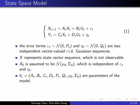
State Space Model

{Xt+1 = AtXt + BtUt + εt

Yt = CtXt + DtUt + ηt(1)

the error terms εt ∼ N (0,Pt) and ηt ∼ N (0,Qt) are twoindependent vector-valued i.i.d. Gaussian sequences.X represents state vector sequence, which is not observable.X0 is assumed to be N (µ0,Σ0), which is independent of εtand ηt .θt = (At ,Bt ,Ct ,Dt ,Pt ,Qt , µ0,Σ0) are parameters of themodel.

Dexiong Chen, Chia-Man Hung 5 / 23

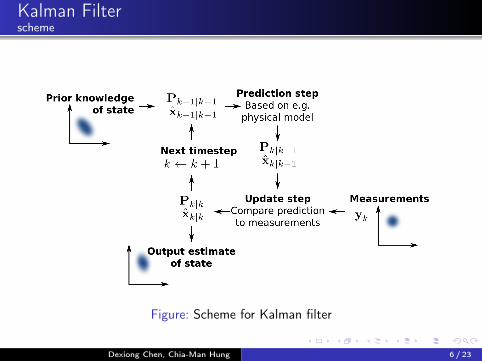
Kalman Filterscheme

Figure: Scheme for Kalman filter

Dexiong Chen, Chia-Man Hung 6 / 23

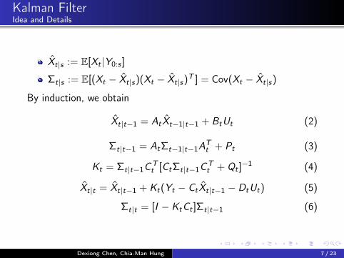
Kalman FilterIdea and Details

Xt|s := E[Xt |Y0:s ]

Σt|s := E[(Xt − Xt|s)(Xt − Xt|s)T ] = Cov(Xt − Xt|s)

By induction, we obtain

Xt|t−1 = AtXt−1|t−1 + BtUt (2)

Σt|t−1 = AtΣt−1|t−1ATt + Pt (3)

Kt = Σt|t−1CTt [CtΣt|t−1C

Tt + Qt ]

−1 (4)

Xt|t = Xt|t−1 + Kt(Yt − CtXt|t−1 − DtUt) (5)

Σt|t = [I − KtCt ]Σt|t−1 (6)

Dexiong Chen, Chia-Man Hung 7 / 23

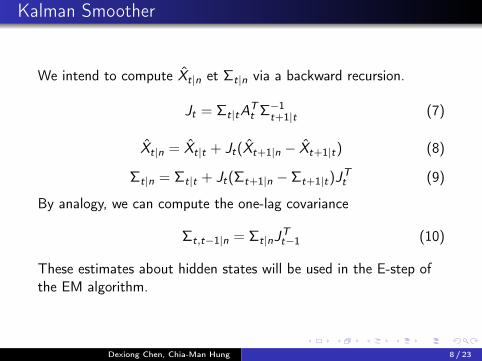
Kalman Smoother

We intend to compute Xt|n et Σt|n via a backward recursion.

Jt = Σt|tATt Σ−1

t+1|t (7)

Xt|n = Xt|t + Jt(Xt+1|n − Xt+1|t) (8)

Σt|n = Σt|t + Jt(Σt+1|n − Σt+1|t)JTt (9)

By analogy, we can compute the one-lag covariance

Σt,t−1|n = Σt|nJTt−1 (10)

These estimates about hidden states will be used in the E-step ofthe EM algorithm.

Dexiong Chen, Chia-Man Hung 8 / 23

1 State Space Model and Kalman Filter

2 EM Algorithm

3 Data Challenge: Prediction of energy consumption

Dexiong Chen, Chia-Man Hung 9 / 23

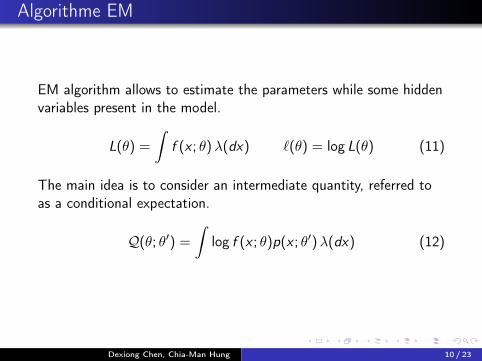
Algorithme EM

EM algorithm allows to estimate the parameters while some hiddenvariables present in the model.

L(θ) =

∫f (x ; θ)λ(dx) `(θ) = log L(θ) (11)

The main idea is to consider an intermediate quantity, referred toas a conditional expectation.

Q(θ; θ′) =

∫log f (x ; θ)p(x ; θ′)λ(dx) (12)

Dexiong Chen, Chia-Man Hung 10 / 23

EM Algorithm

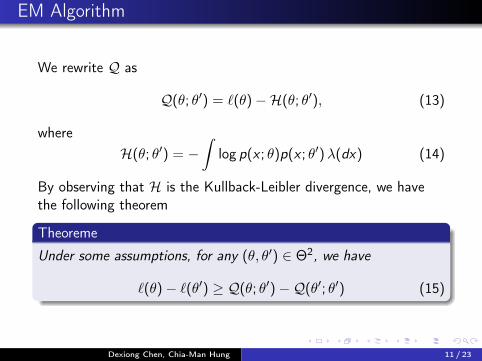
We rewrite Q as

Q(θ; θ′) = `(θ)−H(θ; θ′), (13)

whereH(θ; θ′) = −

∫log p(x ; θ)p(x ; θ′)λ(dx) (14)

By observing that H is the Kullback-Leibler divergence, we havethe following theorem

Theoreme

Under some assumptions, for any (θ, θ′) ∈ Θ2, we have

`(θ)− `(θ′) ≥ Q(θ; θ′)−Q(θ′; θ′) (15)

Dexiong Chen, Chia-Man Hung 11 / 23

EM Algorithm

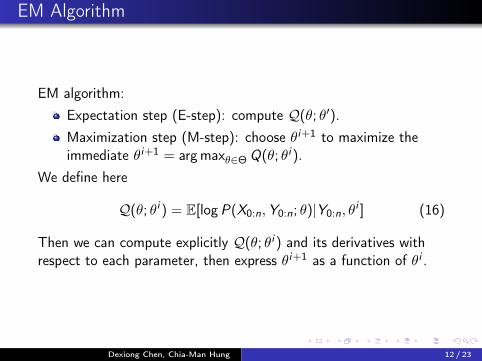
EM algorithm:Expectation step (E-step): compute Q(θ; θ′).Maximization step (M-step): choose θi+1 to maximize theimmediate θi+1 = argmaxθ∈Θ Q(θ; θi ).

We define here

Q(θ; θi ) = E[logP(X0:n,Y0:n; θ)|Y0:n, θi ] (16)

Then we can compute explicitly Q(θ; θi ) and its derivatives withrespect to each parameter, then express θi+1 as a function of θi .

Dexiong Chen, Chia-Man Hung 12 / 23

1 State Space Model and Kalman Filter

2 EM Algorithm

3 Data Challenge: Prediction of energy consumption

Dexiong Chen, Chia-Man Hung 13 / 23

Problem and Data

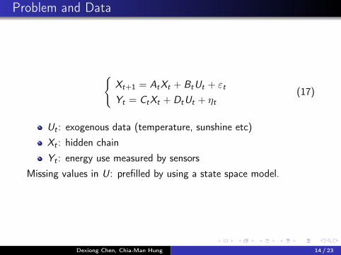
{Xt+1 = AtXt + BtUt + εt

Yt = CtXt + DtUt + ηt(17)

Ut : exogenous data (temperature, sunshine etc)Xt : hidden chainYt : energy use measured by sensors

Missing values in U: prefilled by using a state space model.

Dexiong Chen, Chia-Man Hung 14 / 23

Strategy 1: One Regime Model

We apply directly the model to the problem{Xt+1 = AXt + ε

Yt = CXt + DUt + η(18)

Dexiong Chen, Chia-Man Hung 15 / 23

Strategy 1: One Regime Model

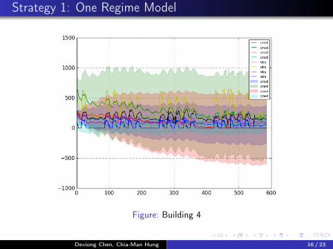
Figure: Building 4

Dexiong Chen, Chia-Man Hung 16 / 23

Strategy 2: Multi-regime Model

{Xt+1 = Aσ(t)Xt + ε

Yt = Cη(t)Xt + Dη(t)Ut + η(19)

We divided states into different groups according to their regime. Itis a particular case of time-variant state-space model.

An instance choice of regimes: “night”, “day”, “day-to-night”,“night-to-day” and “weekend”.Remark: when applying the EM algorithm for this model, wecompute the empirical average respectively over each regimeperiod to estimate parameters belonging to this regime.

Dexiong Chen, Chia-Man Hung 17 / 23

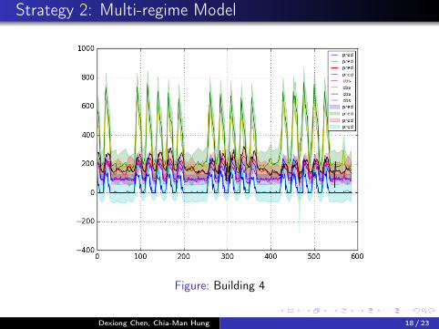
Strategy 2: Multi-regime Model

Figure: Building 4

Dexiong Chen, Chia-Man Hung 18 / 23

Strategy 3: Two-lag Multi-Regime Model

We replace Ut by Ut = (Ut ,Ut−1) in the previous model,{Xt+1 = Aσ(t)Xt + ε

Yt = Cη(t)Xt + Dη(t)Ut + η(20)

Dexiong Chen, Chia-Man Hung 19 / 23

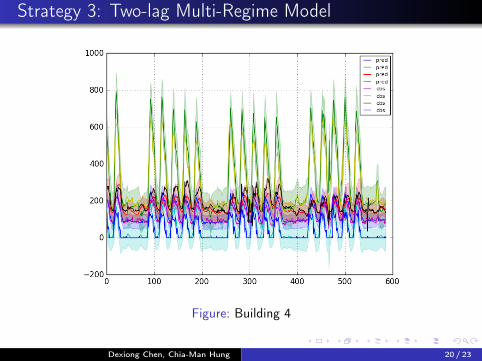
Strategy 3: Two-lag Multi-Regime Model

Figure: Building 4

Dexiong Chen, Chia-Man Hung 20 / 23

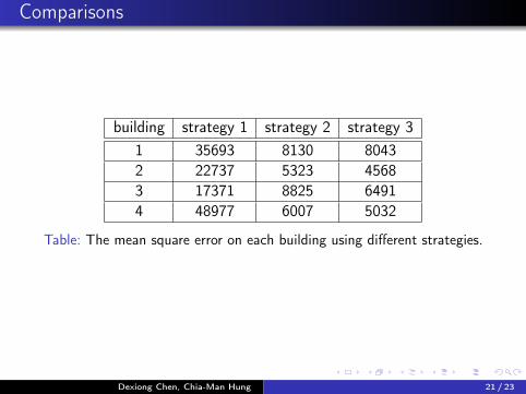
Comparisons

building strategy 1 strategy 2 strategy 31 35693 8130 80432 22737 5323 45683 17371 8825 64914 48977 6007 5032

Table: The mean square error on each building using different strategies.

Dexiong Chen, Chia-Man Hung 21 / 23

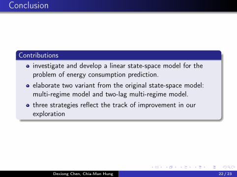
Conclusion

Contributionsinvestigate and develop a linear state-space model for theproblem of energy consumption prediction.elaborate two variant from the original state-space model:multi-regime model and two-lag multi-regime model.three strategies reflect the track of improvement in ourexploration

Dexiong Chen, Chia-Man Hung 22 / 23

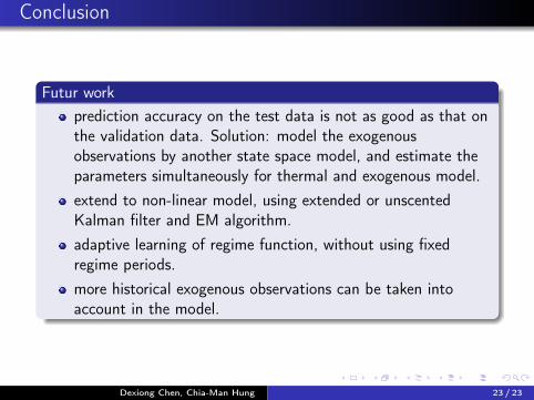
Conclusion

Futur workprediction accuracy on the test data is not as good as that onthe validation data. Solution: model the exogenousobservations by another state space model, and estimate theparameters simultaneously for thermal and exogenous model.extend to non-linear model, using extended or unscentedKalman filter and EM algorithm.adaptive learning of regime function, without using fixedregime periods.more historical exogenous observations can be taken intoaccount in the model.

Dexiong Chen, Chia-Man Hung 23 / 23