stability of nonlinear filters: a survey -...
TRANSCRIPT
STABILITY OF NONLINEAR FILTERS: A SURVEY
PAVEL CHIGANSKY
Abstract. Filtering deals with the optimal estimation of signals from their noisy obser-vations. The standard setting consists of a pair of random processes (X,Y ) = (Xt, Yt)t≥0,where the signal component X is to be estimated at a current time t > 0 on the basis ofthe trajectory of Y , observed up to t. Under the minimal mean square error criterion,the optimal estimate of Xt is the conditional expectation E(Xt|Y[0,t]). If both X and(X,Y ) are Markov processes, then the conditional distribution πt(A) = P (Xt ∈ A|Y[0,t]),A ⊆ R satisfies a recursive equation, called filter, which realizes the optimal fusion of thea priori statistical knowledge about the signal and the a posteriori information borne bythe observation path.
The filtering equation is to be initialized by the probability distribution ν of the signalat time t = 0. Suppose ν is unknown and another reasonable probability distribution νis used to start the filter. As the corresponding solution πt(·) differs from the optimalπt(·), the natural question of stability arises: what are the conditions in terms of thesignal/observation parameters to guarantee limt→∞ ∥πt−πt∥ = 0 in an appropriate sense? The article discusses the recent progress in solving this stability problem, which turnsto be quite interesting and, sometimes, counterintuitive.
Contents
1. A fast-forward introduction 21.1. Hidden Markov Models 21.2. Ergodicity of the filtering process 31.3. Stability of the filtering equation 51.4. What does this survey leave out ? 82. Nonlinear filtering: a brief overview 92.1. Filtering in discrete time 92.2. Filtering in continuous time 133. Filtering stability and ergodicity 183.1. The Hilbert projective metric approach 183.2. The Lyapunov exponents approach 243.3. Conditional time reversal 33References 38
Date: August, 2006.Key words and phrases. nonlinear filtering, hidden Markov models, stability, Lyapunov exponents,
Hilbert projective metric, Birkhoff contraction coefficient, ergodicity, time reversal.These lecture notes have been prepared for the series of talks, delivered by the author at Coloquio Inter-
institucional (CBPF - IMPA - UFF - UFRJ) Modelos Estocasticos e Aplicacoes and Laboratorio Nacionalde Computacao Cientifica, Petropolis, Brazil in August, 2006 upon the invitation of Prof. Jack Baczynski.
1
2 PAVEL CHIGANSKY
1. A fast-forward introduction
1.1. Hidden Markov Models. Consider a Markov chain X = (Xn)n≥0 with values in afinite alphabet S = a1, ..., ad, the transition probabilities λij := P
(Xn = aj |Xn−1 = ai
)and initial distribution νi := P(X0 = ai), i, j = 1, ..., d. Let the observation sequenceY = (Yn)n≥1 be generated by
Yn =
d∑i=1
1Xn=aiξn(i), n ≥ 1, (1.1)
where ξ = (ξn)n≥1 is a sequence of i.i.d. random vectors, independent of X. This settingis usually viewed as a model of a noisy channel, which emits a realization of the randomvariable ξn(i), each time the symbol ai is transmitted. The entries of the vector ξ1 areassumed to be independent and to have known probability densities gi(y), i = 1, ..., d withrespect to some reference σ-finite measure ψ(dy) (e.g. the Lebesgue measure on R orpurely atomic measure).
Having observed the trajectory of Y up to time n ≥ 0, it is required to estimate the stateof the signal Xn on the basis of the observations in an optimal way. The main buildingblock in the solution of this estimation problem under various optimization criteria areconditional probabilities πn(i) = P(Xn = ai|F Y
n ), i = 1, ..., d, where F Yn = σY1, ..., Yn.
For example, the maximum a posteriori probability (MAP) estimate of Xn given F Yn is
Xmapn := argmaxai∈Sπn(i)
and it is optimal in the sense of minimizing the error probability of guessing the state ofXn given the realization of the trajectory Y1, ..., Yn:
infζn∈L∞(Ω,FY
n ,P)P(Xn = ζn
)= P
(Xn = Xmap
n
)= 1− Emax
ai∈Sπn(i) (1.2)
Another criterion is minimizing the mean square error (MSE), under which the optimal
estimate is the conditional expectation Xmsen = E
(Xn|F Y
n ) =∑d
i=1 aiπn(i):
infζn∈L2(Ω,FY
n ,P)E(Xn − ζn
)2= E
(Xn − Xmse
n
)2= E
( d∑i=1
a2iπn(i)−( d∑
i=1
aiπn(i))2)
(1.3)
The vector of conditional probabilities πn satisfies the following filtering equation (es-sentially the recursive Bayes formula):
πn =G(Yn)Λ
∗πn−1∣∣G(Yn)Λ∗πn−1
∣∣ , π0 = ν, (1.4)
where G(y) is a diagonal matrix with entries gi(y), i = 1, ..., d, Λ∗ is the transposed matrixof the transition probabilities and | · | denotes the ℓ1-norm, i.e. |x| =
∑i |xi|, x ∈ Rd.
The model described above is a particular instance of the so called Hidden MarkovModels. The finite state space is special, because many related statistical problems haveefficient closed form solutions. For example, the aforementioned state estimation problemis completely solved in an efficient way by iterating the equation (1.4). Another familiarspecial case is the linear Gaussian systems, for which the conditional distribution of Xn
3
given F Yn is Gaussian, with the mean and covariance satisfing the celebrated Kalman fil-
tering equations. In the general case, the filtering problem, i.e. calculating the conditionaldistribution of Xn given F Y
n , is more complicated and less efficient. The solution is givenin the form of an infinite dimensional recursive equation for conditional distribution or itsdensity. Usually it is used as the basis for efficiently realizable approximate algorithms(particle filters, etc.) The first part of this minicourse is intended as a self contained briefpresentation of the filtering theory both in discrete and continuous time settings.
The second part will focus on a more recent research in filtering, namely stability ofthe nonlinear filtering equation with respect to its initial conditions, ergodicity of thefiltering process, robustness with respect to the model parameters, etc. To make thingsmore concrete and transparent, we will use the equation (1.4) as a toy model. In spite ofits seemingly simple structure, this equation nevertheless features much of the essentialcomplexity of the problem. On the other hand, it is one of the few genuine nonlinearfiltering equations of significant practical importance.
1.2. Ergodicity of the filtering process. Does the estimation error converge to a steadystate ? Do the limits as n→ ∞ of the performance indices in (1.2) and (1.3) exist and ifyes, are they independent of ν ?
Clearly the answers to both questions would be affirmative, if the distribution of πnconverges to a unique distribution over M. Using the properties of conditional expecta-tions, one can verify that the random sequence π = (πn)n≥0 is a Markov process withvalues in the simplex Sd−1. Then the question reduces to whether π = (πn)n≥0 is anergodic process, i.e. it has an invariant measure M and this measure is unique. While theexistence of such measures even in more general situations can be often established usingthe Markov property of the filter, the uniqueness issue turns to be quite nontrivial and infact still lacks a complete answer!
The common intuition suggests that the filtering process π inherits ergodicity from thesignal X itself. Recall that, by definition, a finite state Markov chain X is ergodic if thelimits µi := limn→∞ P(Xn = ai) exist, are positive and do not depend on ν. A chain isergodic if and only if its transition matrix is q-primitive, i.e. there is an integer q ≥ 1,such that the entries of Λq are positive.
Ergodicity of π for ergodic chains X was conjectured by D.Blackwell in [11] (1957),who studied these models in a particularly simple (or as we now realize quite nontrivial!)case, when the observation sequence is formed by a deterministic function h : S 7→ R ofthe signal, i.e. Yn = h(Xn). The original motivation of D.Blackwell was the search fora simple formula for the entropy rate of Y . He did find a formula, but it turned to befar from being simple, as it involved averaging with respect to M (the invariant measureof π) and this in turn had a remarkably complicated structure (e.g. it may be singularwith respect to the Lebesgue measure on Sd−1 yet having no atoms). D.Blackwell was notconcerned primarily with the uniqueness of this measure, as he dealt with the stationary(X,Y ). However to find M one had to solve the corresponding integral equation and thisis where the uniqueness matter showed up.
This conjecture was proven to be false by T.Kaijser in [37] (1975), who pointed outthat an appropriate counterexample was already there in [11], Blackwell’s own paper!This counterexample turns to be quite illuminating as it demonstrates several relevant
4 PAVEL CHIGANSKY
surprising features - we will use its particular version, independently rediscovered in [31](see also [8]).
Example 1.1. Consider a chain with four states S = 1, 2, 3, 4, the following transitionmatrix
Λ =
12
12 0 0
0 12
12 0
0 0 12
12
12 0 0 1
2
and initial distribution ν. The entries of Λ3 are positive and hence the chain is ergodic.Assume that the observation sequence is defined by Yn = 1Xn∈1,3. Notice that, havingobserved the trajectory of Y till time n, one can recover exactly the transitions of Xbetween the groups of states 1, 3 ↔ 2, 4. However it is impossible to tell which one ofthe states within 1, 3 (or 2, 4) the chain actually resides. The filtering recursion (1.4)in this case reads1
πn(1) =(πn−1(4) + πn−1(1)
)Yn
πn(2) =(πn−1(1) + πn−1(2)
)(1− Yn)
πn(3) =(πn−1(2) + πn−1(3)
)Yn
πn(4) =(πn−1(3) + πn−1(4)
)(1− Yn)
(1.5)
subject to π0 = ν. It is not hard to see that πn may take values among the following eightvectors
ϕ1 =
ν1 + ν4
0ν2 + ν3
0
, ϕ2 =
0
ν1 + ν40
ν2 + ν3
, ϕ3 =
ν2 + ν3
0ν1 + ν4
0
, ϕ4 =
0
ν2 + ν30
ν1 + ν4
,
ϕ5 =
0
ν1 + ν20
ν3 + ν4
, ϕ6 =
ν3 + ν4
0ν1 + ν2
0
, ϕ7 =
0
ν3 + ν40
ν1 + ν2
, ϕ8 =
ν1 + ν2
0ν3 + ν4
0
and that Yn form an i.i.d. symmetric binary sequence. Hence the invariant measure of πis uniform over these eight points of Sd−1:
M(du) =1
8δϕ1(du) + ...+
1
8δϕ8(du),
and clearly depends on ν. Sufficient conditions for ergodicity of π in Blackwell’s settingwere derived by T.Kaijser [37] and recently significantly improved by F.Kochman andJ.Reeds, [44]. It is still unclear whether the conditions of [44] are also necessary.
Virtually the same kind of question was independently addressed by H.Kunita in [45](1971) in the continuous time setting. The signal was assumed to be an ergodic Markov
1formally the reference measure ψ(dy) = δ0(dy) + δ1(dy) and the densities are g1(y) = g3(y) = y
and g2(y) = g4(y) = 1 − y
5
process with values in a compact real subset S ⊆ R, the transition semigroup (Pt)t∈R+ andthe initial distribution ν. The observation process was assumed to satisfy
Yt =
∫ t
0h(Xs)ds+Bt,
with the Brownian motion (Wiener process) B, independent of X and bounded functionh. The conditional measure process πt(A) := P(Xt ∈ A|F Y
t ) satisfies a stochastic partialintegro-differential equation (see (2.11) below), which is initialized by the distribution ν.H.Kunita posed the question (πt(f) :=
∫S f(x)πt(dx))
Does the limit limt→∞
E(f(Xt)− πt(f)
)2exist and is it unique ? (1.6)
for any continuous and bounded function f . The main result of [45] is that this limitexists and is unique, if the signal is a Feller-Markov process, whose tail σ-algebra FX
∞ =∩t≥0 FX
[t,∞) is P-a.s. empty. Recently a serious gap in the proof of this claim has been dis-
covered in [8] (2004) (see Section 3.3 below) and currently its validity remains a challengingopen problem.
1.3. Stability of the filtering equation. A different but of course related question of“steady state” behavior was posed by B.Delyon and O.Zeitouni in [31] (1989). Supposethat the actual distribution of X0, needed to initialize the recursion (1.4), is unknown. Itis then reasonable to start the filter from some other probability distribution (e.g. uniformon S) and ask whether the obtained solution, denoted hereafter by πn, will be close tothe optimal one πn for large enough n. It is not immediately clear that an arbitraryprobability distribution can be used to start (1.4), without causing an ambiguity and infact some care should be taken to avoid this kind of pathology. As we will see later, thecondition ν ≪ ν (i.e. νi = 0 =⇒ νi = 0) is sufficient for ν to be a valid initialization for(1.4). The question is what are the conditions in terms of the model parameters, i.e. Λ,gi(u)’s and (ν, ν), for the filter to be stable in the sense∥∥πn − πn
∥∥ :=d∑
i=1
|πn(i)− πn(i)|P−a.s.−−−−→n→∞
0, (1.7)
where ∥ · ∥ denotes the total variation norm, i.e. ∥x∥ =∑d
i=1 |xi|.The aforementioned counterexample shows that the filtering equation may not be stable,
even if the signal is ergodic, namely for (1.5)∥∥πn − πn∥∥ ≥ C > 0, ∀n,
where C is a constant depending on (ν, ν).The relation between the stability of (1.4) and ergodicity of the process π has been
established by D.Ocone and E.Pardoux in [59]: in a quite general setting, the affirmativeanswer to (1.6) implies the stability of the filter in the sense (cf. (1.7))
limt→∞
E(πt(f)− πt(f)
)2= 0, for continuous and bounded functions f, (1.8)
if ν ≪ ν and the signal X is ergodic. Unfortunately in view of the gap in the proofof (1.6) in [45] this does not provide any useful information about (1.8) in terms of themodel. Clearly such type of convergence is weaker than (1.7), however currently (1.8) is

6 PAVEL CHIGANSKY
only known as an implication of this stronger convergence (with the only exceptions forsome special cases as in [27], [25]).
The most significant progress in establishing (1.7) has been accomplished during thelast decade by addressing the problem in even stronger form, namely studying the thelimit2:
γ := limn→∞
1
tlog∥∥πn − πn
∥∥. (1.9)
Negativity of this limit, if exists, implies (1.7). Moreover the value of γ quantifies therate of convergence. The problem was first addressed in this form yet in [31], but thereal progress has been made by R.Atar and O.Zeitouni in [5], [6] (1997). These papersintroduced two different approaches to calculation of γ: the Hilbert projective distanceand Lyapunov exponents techniques. Deferring the detailed discussion of the method untillater, let us briefly review the consequences as applied to the finite state filtering problemunder consideration.
The limit γ in (1.9) exits under mild conditions (essentially ergodicity of X and certainintegrability of the noise densities). Moreover it is a random variable, which takes valuesin a finite set of real numbers, including −∞, depending on3 the initial conditions (ν, ν).Though exact calculation of γ seems to be impossible4, certain information about it canbe gained in the form of upper and lower bounds.
Without any restrictions on the noise densities gi(u), the following upper bound5 holds
γ ≤ −λ∗λ∗, (1.10)
where λ∗ := mini,j λij and λ∗ := maxi,j λij . The latter means that the filter is stable,if all the transition probabilities are strictly positive, i.e. λ∗ > 0. The latter property,sometimes referred in the literature as the mixing property6, is clearly much more strongerthan just ergodicity, and thus the filter does inherit stability from the signal regardlessof the observations structure, but of a rather strong type. In fact (1.10) holds even non-asymptotically:
∥πn − πn∥ ≤ C exp(− λ∗λ∗n), n ≥ 1,
with C > 0 depending on (ν, ν) (more bounds of the same spirit were reported in [51, 50],[24]). On the other hand, Example 1.1 shows that just ergodicity of X is not enough.Then how “much” ergodicity is really required to guarantee filter stability? The exactanswer is not known yet. It turns out that if one of the rows of Λ has all positive entriesand the chain is ergodic, then
γ ≤ −λ⋄λ∗, (1.11)
2all the statements involving random variables are understood to hold P-a.s. as usually3in the “telegraphic signal” case d = 2, γ is independent of (ν, ν). In the general case d > 2, the actual
dependence on the initial condition remains unclear4except for the case d = 2 in continuous time - see [22]5in fact a slightly more tight bound holds, but we prefer to give its simple version at this point to
emphasize the pros and cons6λ∗ > 0 does indeed imply that X is a mixing in the usual sense, but this condition is not necessary for
the chain to be mixing, even when the state space is continuum
7
with λ⋄ :=∑d
i=1 µiminj =i λij (recall that µ is the stationary distribution of Xn). Theproof of (1.11) requires a completely different argument (certain conditional time reversalin P.Baxendale et al [8], P.Ch. and R.Liptser [24]).
Another appealing fact is that the filter is stabilized by noise. Namely, let Y be gener-ated by
Yn = h(Xn) + σξn,
where σ is a constant, h : S 7→ R is a deterministic function and ξ = (ξn)n≥1 is a Gaussiani.i.d. sequence. Then the results of [6] imply that for any σ = 0, γ < 0 and thus the filteris stable. Moreover the following asymptotic bounds as σ → 0 hold (hereafter we writeγ(·) to emphasize its dependence on the relevant parameter)
limσ→0
σ2γ(σ) ≤ −1
2
d∑i=1
µiminj =i
(h(ai)− h(aj)
)2(1.12)
limσ→0
σ2γ(σ) ≥ −1
2
d∑i=1
µi
d∑j=1
(h(ai)− h(aj)
)2. (1.13)
The upper bound (1.12) suggests that the filtering stability is improved as the noise in-tensity decreases, if there is at least one unique point in the image of S under h. Indeed,Blackwell’s counterexample hints that γ(σ) may converge to zero as σ → 0, which wasnumerically tested yet in [31]. In the strong noise regime the filter turns to be as stableas the signal itself:
limσ→∞
γ(σ) ≤ infm≥1
1
mlog τ(Λm) < 0 (1.14)
where τ(·) is the Birkhoff contraction coefficient (see Section 3.1 below), which is strictlyless than 1 for matrices with positive entries (recall that if X ergodic Λm has positiveentries for some integer m ≥ 1).
Another interesting feature of γ is revealed in the slow switching regime. Let Xε denotethe Markov chain whose transition probabilities are defined via the following scaling (withε ∈ (0, 1))
λεij := P(Xε
n = aj |Xεn−1 = ai
)=
ελij j = i
1− ε∑
ℓ=i λiℓ j = i
Clearly smaller values of ε correspond to the chain with less frequent transitions. This set-ting is in a sense more flexible than the noise scaling, since it allows the greater generality7
of the observations model (1.1). A slight adjustment of the arguments from [6] shows thatγ(ε) remains negative for any ε > 0 under the assumption that gi(u) are bounded andhas the same support. More effort is required (essentially the Furstenberg-Khasminskiiformulae, see [23]) to show that
γ(ε) ≤ −d∑
i=1
µiminj =i
D(gi ∥ gj) + o(1), ε→ 0,
7scaling noise by a multiplicative constant σ, does not always makes sense: e.g. when ξn is purelyatomic
8 PAVEL CHIGANSKY
where D(gi ∥ gj) =∫R gi(u) log
gigj(u)φ(du) are the Kullback-Leibler relative entropies.
This suggests that for small ε, the filter remains stable, if at least one entropy is positive.This effect seems to be an attribution of the finite state space, since it is absent in theKalman filtering setting.
For d = 2 this asymptotic is precise, i.e.
γ(ε) = −µ1D(g1 ∥ g2)− µ2D(g2 ∥ g1) + o(1), ε→ 0.
and γ(ε) turns to be not necessarily monotonic in ε. Namely for a symmetric binary chainwith transition probability λ and Yn = (Xn − ξn)
2 with an i.i.d. binary noise sequence ξ,P(ξ1 = 1) = p,
γ(ε) ≥ −Dp +4λ(log(2)− h(p)
)Dp
ε log ε−1(1 + o(1)
), ε→ 0.
where Dp := p logp
1− p+(1− p) log 1− p
pand h(p) = −p log p− (1− p) log(1− p). As the
second order term is positive, the formula (3.22) suggests that the limit −Dp is approachedfrom above. On the other hand, it can be easily seen that γ(ε′) = −∞ for ε′ = 1/(2λ).Hence the function γ(ε) has a global maximum at some positive ε⋆ (see Figure 1 on page27), which means that the filtering stability may improve as the signal is slowed downbeyond certain value of ε!
1.4. What does this survey leave out ? Limited by the course time scale, this surveydoes not elaborate some of the results available in the literature (though the author doestry his best to provide a complete bibliography). Here is a brief account of things, whichhave been omitted.
The results and methods mentioned in the Introduction translate without much effort tothe settings with Markov ergodic signals on compact (not necessarily finite) domains (seee.g. [29], [30], [28]). It is possible to push some of the methods to noncompact/nonergodicsettings: some clever arguments appeared in [3], [16], [15], [52], [53] (and more recentvariations on this theme in [32], [74], [60], [61], [43], [42]). However none of the results iseven close to the powerful controllability/observability stability criteria, available in theKalman-Bucy case. Thus the final word in this story is still missing and a completely freshidea may be required to fill this gap.
On the other hand some results, which directly rely or repeat the arguments from [45],are to be revised: [59], [14], [13], [12], [9], [72], [73], [46], [49].
There are some “out of mainstream” interesting results, indicating that (1.8) (or evenweaker stability) may hold for certain function, even when stability in the total variationnorm as (1.7) fails or unknown (see [27], [58], [25]). Sometimes stronger results are possiblein specific situations as e.g. for Benes filters in [57], the noise free signal dynamics [21],etc. (see also [4], [7]). A variational approach of a functional analysis flavor was recentlysuggested by W.Stannat in a series of papers [69, 71, 70].
The stability with respect to initial conditions is naturally related to the robustness ofthe filtering equation with respect to the model parameters over the infinite horizon. Therelated results appeared in [53, 52], [60], [19, 18, 17]. Recently the continuous time casehas been addressed in [26].
9
The rest of this article is organized as follows. Section 2 gives a sketchy overview of thenonlinear filtering theory, which is intended to give a self contained background for thereader, unfamiliar with it. Section 3 gives a detailed presentation of three approaches tofiltering stability and ergodicity, mentioned in the Introduction.
2. Nonlinear filtering: a brief overview
2.1. Filtering in discrete time. The more general filtering problem is formulated asfollows. Let X = (Xn)n∈Z+ be a Markov sequence with values in Rd, transition probabilitydensity λ(x, u):
P(Xn ∈ Γ |FX
n−1
)=
∫Γλ(Xn−1, u)ψ(du), ∀Γ ∈ B(Rd), P− a.s.
where ψ(du) is another σ-finite measure on Rd and initial probability density ν, i.e.
P(X0 ∈ Γ ) =
∫Γν(x)ψ(dx), ∀Γ ∈ B(Rd).
Sometimes, when no confusion is caused, we will write λ(x, du) for λ(x, u)ψ(du) andλ(x, Γ ) for
∫Γ λ(x, u)ψ(du) for brevity and similarly, denote by ν the measure ν(x)ψ(dx)
rather than the density itself.The observation process Y = (Yn)n∈Z+ is assumed to form an i.i.d. random sequence8,
conditioned on X, i.e. for n ≥ 1
P(Yn ∈ Γ |FX
n ∨ F Yn−1
)=
∫Γg(Xn, y)φ(dy), ∀Γ ∈ B(Rℓ), P− a.s.,
where g(x, y) is the observation probability density with respect to a σ-finite referencemeasure φ(dy) on Rℓ. g(x, y) is sometimes referred as the likelihood function.
As a special case, this formulation includes the recursion
Xn = a(Xn−1) + b(Xn−1)ηn
Yn = c(Xn) + d(Xn)ξn,
where η and ξ are independent i.i.d. sequences and a(·), b(·),c(·) and d(·) are functions ofappropriate dimensions. For example, for the scalar linear Gaussian problem (i.e. whena(x) := ax, c(x) := cx, b(x) := b and d(x) := d and when the noises ξ and η are Gaussian)
λ(x, u) =1√2πb
exp
(u− ax)2
2b2
and
g(x, y) =1√2πd
exp
(y − cx)2
2d2
with ψ and φ being the Lebesgue measures on R.
The filtering equation for the general problem propagates the conditional density (withrespect to ψ) of Xn given F Y
n , n ≥ 1
πn(x) =g(x, Yn)
∫Rd λ(u, x)πn−1(u)ψ(du)∫
Rd g(x, Yn)∫Rd λ(u, x)πn−1(u)ψ(du)ψ(dx)
, π0(x) = ν(x), (2.1)
8as before Y0 ≡ 0 is assumed, or in other words FY0 = ∅,Ω
10 PAVEL CHIGANSKY
where
πn(Γ ) :=
∫Γπn(x)ψ(dx) = P
(Xn ∈ Γ |F Y
n
), Γ ∈ B(R).
2.1.1. Finite dimensional filters. The equation (2.1) is infinite dimensional in general,meaning that its solution cannot be parameterized by a finite set of sufficient statistics.For this reason, the general filtering equation is of limited practical value and is usuallyused as the basis for various approximations.
However there are two important classes of systems for which the filter turns to be finitedimensional: the aforementioned finite state Markov chains and the familiar Kalman’slinear Gaussian setting. In the former case, the filtering distribution is just the vectorof conditional probabilities satisfying the d − 1 dimensional recursion (1.4). In the lattercase, i.e. when the signal/observation pair is generated by
Xn = AXn−1 +Bηn
Yn = CXn +Dξn(2.2)
with independent i.i.d. Gaussian noises η = (ηn)n≥1 and ξ = (ξn)n≥1, deterministicmatrices A,B,C and D of appropriate dimensions and Gaussian initial condition X0, in-dependent of η and ξ, the conditional density is Gaussian:
πn(x) =1
(2π)n/2 det(Pn)exp
−1
2(x− Xn)P
−1n (x− Xn)
∗)
with the conditional mean E(Xn|F Y
n ) = Xn and covariance E(Xn − Xn)(Xn − Xn)∗ = Pn
satisfying the Kalman recursions:
Xn = AXn−1 + Pn|n−1C∗(CPn|n−1C
∗ +DD∗)−1(Yn − CAXn−1
)Pn|n−1 = APn−1A
∗ +BB∗
Pn = Pn|n−1 − Pn|n−1C∗(CPn|n−1C
∗ +DD∗)−1CPn|n−1.
These two settings are virtually the only practically important instances of (2.1) (in fact,some other estimation problems for these models turn to be finite dimensional as well -see e.g. [33]).
2.1.2. The reference measure point of view - the Zakai equation. The equation (2.1) isnonlinear, however its solution is obtained by solving the linear Zakai type equation:
ρn(x) = g(x, Yn)
∫Rd
λ(u, x)ρn−1(u)ψ(du), n ≥ 0, (2.3)
subject to ρ0(x) = ν(x), via normalization:
πn(x) =ρn(x)∫
Rd ρn(u)ψ(du). (2.4)
This can be readily verified by induction, however the following “representation” formulaeturn to be useful on their own, in particular in the stability problems under consideration.Let g(y) be a probability density with respect to φ, such that
bothg(y)
g(x, y)and
g(x, y)
g(y)
11
are well defined for each (x, y) ∈ Rd × Rℓ (possibly with the convention 0/0 ≡ 0). Weassume that such a density exists, (which will usually be the case - e.g. any non-vanishingdensity would do for the Kalman model), though its specific choice is of no importance.For a fixed n ≥ 1, introduce the random variable
Zn =
n∏m=1
g(Ym)
g(Xm, Ym)
and define the measure P by means of the Radon-Nikodym derivativedP
dP=: Zn(ω). Since
Zn > 0 P-a.s. and
P(Ω) = EZn = EE
(n∏
m=1
g(Ym)
g(Xm, Ym)
∣∣∣FXn
)=
E
∫Rℓ×...×Rℓ
n∏m=1
g(ym)
g(Xm, ym)
n∏m=1
g(Xm, ym)φ(dy1)...φ(dym) =
E
∫Rℓ×...×Rℓ
n∏m=1
g(ym)φ(dy1)...φ(dym) = 1,
P is a probability measure. Moreover under P, X and Y are independent, X is distributedas under P and Y is an i.i.d. sequence with Y1 having distribution g(y)ψ(dy). Indeed, forany bounded functionals αn : (Rd)n 7→ R and βn : (Rℓ)n 7→ R
Eαn(X)βn(Y ) = Eαn(X)βn(Y )Zn = Eαn(X)E(βn(Y )
n∏m=1
g(Ym)
g(Xm, Ym)
∣∣∣FXn
)=
Eαn(X)E(∫
Rℓ
...
∫Rℓ
βn(y)
n∏m=1
g(ym)
g(Xm, ym)
n∏m=1
g(Xm, ym)φ(dy1)...φ(dyn)∣∣∣FX
n
)=
Eαn(X)
∫Rℓ
...
∫Rℓ
βn(y)
n∏m=1
g(ym)φ(dy1)...φ(dyn) = Eαn(X)Eβn(Y ).
The following lemma derives the transformation of the conditional expectations underequivalent change of measure.
Lemma 2.1. Let P and P be a pair of equivalent9 measures on (Ω,F ) and G be a sub-σ-
algebra of F , then for any random variable α with E|α| <∞
E(α∣∣G ) = E
(αdP
dP(ω)|G)
E(dPdP(ω)|G
) .Proof. One has to check that for any G -measurable bounded random variable θ
E
(α−
E(αdP
dP(ω)|G)
E(dPdP(ω)|G
) )θ = 0.
9i.e. P ≪ P and P ≪ P
12 PAVEL CHIGANSKY
The latter indeed holds:
EE(αdP
dP(ω)|G)
E(dPdP(ω)|G
) θ = EdP
dP(ω)
E(αdP
dP(ω)|G)
E(dPdP(ω)|G
) θ = EE(dPdP
(ω)∣∣G)E(αdP
dP(ω)|G)
E(dPdP(ω)|G
) θ =EE(αdP
dP(ω)|G
)θ = Eαθ
dP
dP(ω) = Eαθ.
SincedP
dP= Z−1
n , by this lemma for any Γ ∈ B(Rd)
πn(Γ ) = P(Xn ∈ Γ |F Y
n
)=
E(1Xn∈ΓZ
−1n |F Y
n
)E(Z−1n |F Y
n
) =
E(1Xn∈Γ
∏nm=1
g(Xm, Ym)
g(Ym)
∣∣∣F Yn
)E(∏n
m=1
g(Xm, Ym)
g(Ym)
∣∣∣F Yn
) =E(1Xn∈Γ
∏nm=1 g(Xm, Ym)|F Y
n
)E(∏n
m=1 g(Xm, Ym)|F Yn
) †=
∫1xn∈Γ
∏nm=1 g(xm, Ym)µX(dx)∫ ∏n
m=1 g(xm, Ym)µX(dx),
where the independence of X and Y under P was used and µX(dx) denotes the probabilitydistribution10 of X = (Xn)n∈Z+ . Using the Markov property of X, the numerator of the
latter expression is found to satisfy the equation (2.3) (recall that under P, X and Y areindependent). Namely, let∫
1xn∈Γ
n∏m=1
g(xm, Ym)µX(dx) =: ρn(Γ ), n ≥ 1,
then
ρn(Γ) =
∫1xn∈Γ
n∏m=1
g(xm, Ym)µX(dx) = E(1Xn∈Γ
n∏m=1
g(Xm, Ym)∣∣∣F Y
n
)=
E[ n−1∏m=1
g(Xm, Ym)E(1Xn∈Γg(Xn, Yn)
∣∣∣F Yn ∨ FX
n−1
)∣∣∣F Yn
]=
E[ n−1∏m=1
g(Xm, Ym)
∫Γg(u, Yn)λ(Xn−1, u)ψ(du)
∣∣∣F Yn
]=∫
Γg(u, Yn)
(∫Rλ(x, u)ρn−1(dx)
)ψ(du).
ρn is a measure valued random sequence, called unnormalized conditional distribution.
10more formally the induced measure on (Rd)∞
13
2.2. Filtering in continuous time. Both the problem formulation and its solution ismuch more delicate in the continuous time, due to the lack of the “white noise” analoguefor the discrete time i.i.d. sequence. This goal of this section is to give a very superficialguide to the subject. For the complete and consistent presentation the reader is referredto [55, 54] (other texts are [38], [33])
Let X = (Xt)t∈R+ be a Markov process with trajectories in the space of functions[0, T ] 7→ R continuous from the right and having limits from the left (abbreviated in Frenchas cadlag functions). This space is denoted by D[0,T ] and is to a complete separable metric(i.e. Polish) space, when endowed with the Skorokhod metric. The transition semigroupand the initial distribution of the process are assumed to be known. The observationprocess Y = (Yt)t∈R+ is given by
Yt =
∫ t
0h(Xs)ds+Bt, (2.5)
where h is a continuous R 7→ R function and B = (Bt)t∈R+ is a Brownian motion, inde-pendent of X.
The general filtering equation for the conditional distribution of Xt, given F Yt =
Ys, s ≤ t can be derived either via the martingale representation theorem or the refer-ence measure approach. We omit the discussion of the former approach (see e.g. Chapter8, [55]) and outline the main idea of the later. The key tool is the Girsanov change ofmeasure.
Theorem 2.2 (I.Girsanov). Consider a Brownian motion B, defined on a filtered proba-bility space11 (Ω,F ,Ft,P) and define
Zt := exp
(∫ t
0αsdBs −
1
2
∫ t
0α2sds
),
where αs is a random process, such that12 the Ito integral with respect to B is well defined.Assume13 that EZT = 1 and define a probability measure P on (Ω,F ) by means of the
Radon-Nikodym derivativedP
dP= ZT (ω). Then the process Vt = Bt−
∫ t0 αsds is a Brownian
motion on (Ω,F ,Ft, P).
Proof. (sketch) Since the trajectories of V are continuous functions, the claim holds bythe Levy theorem if for any λ ∈ R
E(eiλ(Vt−Vs)
∣∣Fs
)= e−
12λ2(t−s)2 .
11all the processes are adapted to Ft: in particular one may take Ft := FBt ∨ Fα
t
12essentially α should be adapted to FBt and satisfy P
( ∫ T
0α2sds <∞
)= 1
13by the Ito formula Zt satisfies the SDE Zt = 1 +∫ t
0ZsαsdBs. This however does not guarantee
that EZT = 1, i.e. the expectation of the stochastic integral may be nonzero. If the Novikov condition is
satisfied, i.e. E exp(
12
∫ T
0α2sds
)<∞, then semimartingale Zt is also a martingale, i.e. EZT = 1 and thus
it can be used to define a change of probability measure
14 PAVEL CHIGANSKY
For simplicity let’s verify the latter for s = 0 (the proof for s > 0 is essentially the same).By the Ito formula Ut := eiλVt satisfies
dUt = iλUtdVt −λ2
2Utdt.
Since EZT = 1,
EeiλVt = EZT eiλVt = EeiλVtE(ZT |Ft) = EeiλVtZt = EUtZt
Once again using the Ito formula we get:
d(UtZt
)=UtdZt + ZtdUt + iλUtZtαtdt =
UtZtαtdBt + iλUtZtdVt −λ2
2UtZtdt+ iλUtZtαtdt =
UtZtαtdBt + iλUtZtdBt − iλUtZtαtdt−λ2
2UtZtdt+ iλUtZtαtdt,
(2.6)
and taking the expectation from both sides one gets the ODE for Ψ(t) := EeiλVt = EUtZt
d
dtΨ(t) = −1
2λ2Ψ(t), Ψ(0) = 1,
whose solution gives the required answer.
Back to the filtering problem at hand, introduce
Zt = exp(−∫ t
0h(Xs)dBs −
1
2
∫ t
0h2(Xs)ds
)and define the reference measure by
dP
dP:= ZT (ω).
If e.g. h(Xs) is bounded, then P is a probability measure and by the Girsanov theorem
with αt := −h(Xt), the process Yt is a Brownian motion under the probability P. Moreover
independence of X and B under P translates to the independence of X and Y under P. Infact, a stronger version of the Girsanov’s theorem holds in this case, namely the processYt is a Brownian motion under the conditional measure given FX
T . By Lemma 2.1
E(eiλVt |FX
T
)=
E(UtZT |FX
T
)E(ZT |FX
T ).
Recall that if B is independent of a σ-algebra G ⊆ F , then14 E( ∫ t
0 αsdBs
∣∣G) = 0. The
martingale Zt satisfies
Zt = 1−∫ t
0Zsh(Xs)dBs (2.7)
14this is easily verified for simple functions α and extended to the general case by a limiting procedure
15
and since B is independent of FXT , we have E
(ZT |FX
T ) = 1. Similarly
E(UtZT |FX
T
)= E
(UtE(ZT |FX
T ∨ FBt )∣∣FX
T
)=
E(UtE
(Zt −
∫ T
th(Xs)ZsdBs|FX
T ∨ FBt
)∣∣FXT
)= E
(UtZt|FX
T
)and in turn by (2.6)
E(eiλVt |FX
T
)= E
(UtZt|FX
T
)= e−
12λ2t2 .
Hence for any measurable bounded functionals F : D[0,T ] 7→ R and G : C[0,T ] 7→ R
EF (X)G(Y ) = EF (X)E(G(Y )|FX
T
)= EF (X)EG(B),
i.e. X and Y are independent under P. Finally
EF (X) = EZTF (X) = EF (X)E(ZT |FX
T
)= EF (X)
i.e. the distribution of X remains unaltered under the change of measure.To summarize, under the reference measure P, X and Y are independent, Y is a Brow-
nian motion and X has the same distribution as under P. Note that since P ∼ P,
dP
dP(ω) = Z−1
T = exp(∫ t
0h(Xs)dBs +
1
2
∫ t
0h2(Xs)ds
)=
exp(∫ t
0h(Xs)dYs −
1
2
∫ t
0h2(Xs)ds
)Then by Lemma 2.1,
P(Xt ∈ Γ|F Y
t
)=
E(1Xt∈Γ exp
( ∫ t0 h(Xs)dYs − 1
2
∫ t0 h
2(Xs)ds)∣∣∣F Y
t
)E(exp
( ∫ t0 h(Xs)dYs − 1
2
∫ t0 h
2(Xs)ds)∣∣∣F Y
t
).
Since under P, X and Y are independent this can be rewritten in a more compact form,known as the Kallianpur-Striebel representation formula
P(Xt ∈ Γ|F Y
t
)=
∫D[0,T ]
1xt∈ΓΦt
(x, Y (ω)
)µX(dx)∫
D[0,T ]Φt
(x, Y (ω)
)µX(dx)
(2.8)
where µX(dx) is the probability measure induced by X on D[0,T ] and15
Φt
(x, Y (ω)
):= exp
(∫ t
0h(xs)dYs −
1
2
∫ t
0h2(xs)ds
).
Now the Markov property of X can be used to deduce a recursive equation for theunnormalized conditional distribution:
ρt(Γ) = E(1Xt∈ΓΦt(X,Y )|F Y
t
).
15i.e. Φt(X,Y ) = Z−1t
16 PAVEL CHIGANSKY
For definiteness, consider the simplest case, when Xt is a Markov chain with values in afinite alphabet S = a1, ..., ad, with transition intensities λij :
P(Xt+δ = aj |Xt = ai
)=
λijδ + o(δ), i = j
1−∑
ℓ =i λiℓδ + o(δ), i = j
and initial distribution ν: νi = P(X0 = ai). Introduce indicators vector process Jt with theentries Jt(i) = 1Xt=ai and let ρt be the vector of unnormalized conditional probabilities:
ρt := E(JtZ
−1t |F Y
t
).
Clearly there is a one-to-one correspondence between X and J (assuming that all ai’s aredifferent). The process Jt is a semimartingale with the decomposition
Jt = J0 +
∫ t
0Λ∗Jsds+Mt,
where Λ∗ is the transposed matrix of transition intensities and M is a (purely discontinu-ous) martingale (with respect to FX
t ). Recall that Z−1t satisfies the equation
dZ−1t = Z−1
t h(Xt)dYt
and apply the Ito formula to the product JtZ−1t :
d(JtZ−1t ) = JtdZ
−1t + Z−1
t dJt = Jth(Xt)Z−1t dYt + Λ∗JtZ
−1t dt+ Z−1
t dMt =
H(JtZ−1t )dYt + Λ∗(JtZ
−1t )dt+ Z−1
t dMt (2.9)
where the equality Jth(Xt) = HJt with16 H = diag(h) was used. Since M is independent
of F Y under P,
E(∫ t
0Z−1s dMs
∣∣F YT
)= 0.
Conditioning both sides of (2.9) on F Yt , one gets the Zakai equation for ρt:
dρt = Λ∗ρtdt+HρtdYt, ρ0 = ν.
This is a linear (more exactly bilinear) SDE with respect to ρt, driven by the observationprocess Yt. It is the continuous time analogue of the recursion (2.3). The conditionalprobabilities πt := E(Jt|F Y
t ) are recovered from ρt by normalization πt = ρt/∥ρt∥, with∥ρt∥ =
∑di=1 ρt(i).
The vector πt satisfies the nonlinear (Wonham) SDE, obtained by applying the Itoformula to ρt/∥ρt∥:
dπt = Λ∗πtdt+(diag(πt)− πtπ
∗t
)h(dYt − πt(h)dt
), π0 = ν, (2.10)
where h is a vector of the values of h on S, πt(h) = ⟨πt, h⟩ =∑d
i=1 h(ai)πt(i) and diag(πt)is a diagonal matrix with entries πt(i), i = 1, ..., d. This is the analogue of the HMM filter(1.4) in continuous time setting.
The process Bt := Yt −∫ t0 πt(h)ds is the innovation Brownian motion with respect to
F Yt under the original measure P. This fact can be established in a much more greater
generality and is the key to the martingale derivation of the equation for πt (which we
16the function h on S is naturally identified with the vector of h(a1),...,h(ad)
17
omit here). This approach allows to derive a general filtering Fujisaki-Kallianpur-Kunitaequation for the conditional distribution of Xt with respect to F Y
t , which is the generalcontinuous time analogue of the filtering recursion (2.1). The FKK equation is the funda-mental result in filtering, defining the evolution of the conditional distribution πt. Beinga measure valued functional stochastic equation, it has a rather complicated form, whichwe do not describe here. The finite dimensional Wonham filter (2.10) is the particularlysimple instance of this equation, which is of practical importance.
In the case when X is a diffusion process
Xt = a(Xt)dt+ b(Xt)dWt,
where W is a Brownian motion, independent of B and a and b are functions with ap-propriate properties, the FKK equation reduces to the functional Kushner-StratonovichSPDE (cf. (2.10)) for the conditional density πt(x) with respect to the Lebesgue measure(if it exists!):
dtπt(x) = L∗πtdt+(h(x)− πt(h)
)πt(x)
(dYt − πt(h)dt
), (2.11)
where L∗ is the infinitesimal operator corresponding to X and πt(h) :=∫R h(x)πt(x)dx.
The corresponding unnormalized conditional distribution in this case has the density17
ρt(x), which satisfies the linear Zakai SPDE
dtρt(x) = L∗ρt(x)dt+ h(x)ρt(x)dYt, ρ0(x) = ν(x). (2.12)
Conditions for existence and uniqueness of the solutions of the filtering equations as wellas their properties are far from being obvious and is a subject of extensive research bothin the past and now. In the particular case of linear system (A, B, C and D are constantmatrices; W and B are independent vector Brownian motions)
dXt = AXtdt+BdWt
dYt = CXtdt+DdBt
subject to a Gaussian X0, the conditional density πt(x) is Gaussian with the mean X andcovariance Pt, satisfying the familiar Kalman-Bucy equations:
dXt = AXtdt+ PtC∗(DD)−1(dYt − hXtdt)
Pt = APt + PtA∗ +BB∗ − PtC
∗(DD)−1CPt,
subject to X0 = EX0 and P0 = E(X0 − X0)(X0 − X0)∗. Finite dimensional realizations
are available for various functionals of (X,Y ) in the LQG and finite state settings (seethe book [33]). Other finite dimensional cases of the filtering equation are known (mostnotably the Benes diffusion case), but their practical value is limited.
17here a measure and its density are denoted by the same letter, as e.g. here ρt(dx) = ρt(x)dx orν(dx) = ν(x)dx.
18 PAVEL CHIGANSKY
3. Filtering stability and ergodicity
This section deals with the stability problem of the nonlinear filtering equation and theergodic properties of its solution. We will restrict the following discussion to the simple(and yet nontrivial!) case of finite state Markov chains in discrete time and will showhow most of the results, presented in the introduction are derived. Further extensions andother results, reported in the literature, are gathered in the bibliography for the readersreference. The main reason for the choice of such simplified treatment is its transparencyand concreteness. Since the “curse of dimensionality” is resolved in this case due tothe finite dimensionality of the signal (and not due to the very special properties of theGaussian processes as in the Klamaa-Bucy setting), many of the results extend to moregeneral settings without major difficulty - essentially to the models with ergodic signalson a compact state space. The nonergodic/noncompact case is more difficult and virtuallyall currently available results combine one of the methods with a “compactification” trick.Regretfully none of them recaptures the well known powerful controllability/observabilityconditions of the Kalman-Bucy linear Gaussian case.
3.1. The Hilbert projective metric approach.
3.1.1. Nonnegative operators acting on nonnegative measures. This section presents theideas from the theory of nonnegative operators, introduced into the filtering stabilityproblem by R.Atar and O.Zeitouni in [6], [5].
Let S ⊆ Rd be a measurable set18 and M+ be the space of nonnegative measures on(S,B(S)
)with the partial order relation p ≼ q if p(A) ≤ q(A) for any measurable A ⊆ S.
The measures p and q are comparable if c1p ≼ q ≼ c2p for some constants c1, c2 > 0. TheHilbert projective distance is defined
h(p, q) = logsupA,q(A)>0 p(A)/q(A)
infA,q(A)>0 p(A)/q(A), p, q ∈ M+ are comparable
and h(p, q) = ∞ otherwise. Clearly two comparable measures p and q are equivalent andvise versa and hence (∥ · ∥∞ is the supremum norm)
h(p, q) = log(∥∥∥dpdq
∥∥∥∞
∥∥∥dqdp
∥∥∥∞
).
It is easy to see that h(p, q) is a nonnegative symmetric function, satisfying the triangleinequality
h(p, q) ≤ h(p, r) + h(r, q), p, q, r ∈ M+.
Also h(p, q) = 0 iff p = cq for some c > 0. The latter property turns (M+, h) into apseudo-metric space. Notice also that on the space of probability (i.e. normalized to 1)measures, h defines a metric on the part of the domain where it takes finite values. Thisis not as innocent as it may seem - e.g. this metric is infinite for Gaussian measures withdifferent means!
The following two properties are important for our purposes:
18the host space is taken to be Rd here for definiteness - more general spaces are possible. Also S can beRd itself. The distinction is made to emphasize in the sequel to distinguish the compact and noncompactstate spaces
19
(p-1) h(p, q) = h(c1p, c2q) for any p, q ∈ M+ and any scalars c1, c2 > 0(p-2) ∥p− q∥ ≤ 2
log(3)h(p, q) for any p, q ∈ Sd−1
The first property is obvious from the definition. The proof of the second one is given e.g.in Lemma 1 in [5].
Let K be a linear positive operator, mapping M+ to itself. The Birkhoff contractioncoefficient is defined as
τ(K) := sup0<h(p,q)<∞
h(Kp,Kq)
h(p, q). (3.1)
τ(K) has the following expression in terms of h-diameter H(K) := supp,q∈M+h(Kp,Kq
)of K:
τ(K) = tanh(H(K)
4
). (3.2)
Moreover, if the operator K is of the integral form
(Kp)(du) :=
∫Sκ(x, u)p(dx)ψ(du),
where κ(x, u) is a nonnegative function (kernel) and ψ is a σ-finite measure, then
H(K) = log ess supx,u,x′,u′
κ(x, u)κ(x′, u′)
κ(x, u′)κ(x′, u), (3.3)
where 0/0 = 1 is assumed and the sup is strict over x and y and ψ-essential over u andu′. Proofs of these facts can be found in Theorem 3 of Chapter XVI in [10] or Theorem 1in [35].
Remark 3.1. In the filtering context, we will be particularly interested in the operatorswith even more specific structure, namely
Kgp := g(u)
∫Sκ(x, u)p(dx)ψ(du),
where g(u) is a nonnegative function (the likelihood). Note that if g(u) is strictly positive,then H(Kg) = H(K). However, Kg is still a strict contraction, regardless of the propertiesof g, if the kernel κ(x, u) satisfies the “mixing” condition, i.e. if some constants κ∗ and κ∗
0 < κ∗ ≤ κ(x, u) ≤ κ∗ <∞.
In this case, (3.3) implies
H(K) ≤ log(κ∗κ∗
)2(3.4)
and consequently
τ(K) ≤ κ∗ − κ∗κ∗ + κ∗
=: τ(K) < 1. (3.5)
As observed in [15] and [52], these inequalities remain valid for Kg as well, since it remainsto be mixing with respect to a different reference measure, namely ψg(du) := g(u)ψ(du):
τ(Kg) ≤ τ(K) < 1. (3.6)
20 PAVEL CHIGANSKY
Example 3.2. For the finite state space S = a1, ..., ad, the above notions read asfollows. The space M+ is just the nonnegative cone of Rd or in other words M+ canbe identified with the vectors from Rd with nonnegative entries. The Hilbert distancebetween p, q ∈ M+ is defined as19
h(p, q) :=
logmaxi pi/qiminj pj/qj
, if p ∼ q
∞, otherwise(3.7)
with the convention 0/0 = 1.Any nonnegative operator on M+ can be represented by a d× d matrix A = (aij) with
nonnegative entries. If A is an allowable matrix, i.e. none of its columns or rows containsonly zeros, then
H(A) = log maxi,j,k,ℓ
aikajℓaiℓajk
.
Notice that if a contains at least one zero entry, then H(K) = ∞ and τ(A) = 1. Otherwise
τ(A) = tanh(H(A)
4
)=
1−√ψ(A)
1 +√ψ(A)
, ψ(A) := mini,j,k,ℓ
aikajℓaiℓajk
∣∣∣ailajk = 0
. (3.8)
Hence τ(A) is strictly less than unity if and only if all the entries of an allowable matrixare nonzero. In particular, with a∗ := minij aij and a∗ := maxij aij ,
log τ(A) ≤ −a∗a∗
and, as the formula (3.8) suggests, for any diagonal matrixD with strictly positive diagonalentries
τ(A) = τ(AD) = τ(DA). (3.9)
If D has some zero diagonal entries, but all the elements of A are positive, then
τ(AD) ≤ a∗ − a∗a∗ + a∗
.
3.1.2. Application to the filtering problem. The following construction will be convenientto use in the sequel. Without loss of generality, we assume that (X,Y ) are coordinateprocesses on the canonical probability space (Ω,F ) =
(R∞×R∞,B(R∞)×B(R∞)
). We
denote by P and P the probability measures, under which (X,Y ) is a Markov processwith the given transition semigroup (i.e. X is a finite state Markov chain with transitionsprobabilities matrix Λ and Y is an i.i.d. sequence conditioned on FX) and X0 is hasdistribution ν and ν respectively. Let PY and PY be the distributions of Y = (Yn)n≥1
under P and P and PYn and PY
n be their restrictions on F Yn = σY1, ..., Yn (i.e. these are
just the probability distributions of the vector Y1, ..., Yn under P and P). Finally let Ps
the probability measure under which (X,Y ) is a stationary process, i.e. when X0 ∼ µ.The n first iterations of (1.4) define a functional Ψn(y) : Rn 7→ Sd−1, which is well
defined on a set of full P-probability. By the Markov property of (X,Y ), the assumptionν ≪ ν implies P ≪ P and hence Ψn(y) is a well defined P-a.s. as well. Note also that for
19p ∼ q stands for equivalence (in the sense of mutual absolute continuity) relation between the measuresp and q. In the finite case, this means that p and q should not vanish at the same indices
21
ergodic X, the invariant measure µ is positive and hence ν ≪ µ for any ν ∈ Sd−1. Thise.g. implies P ≪ Ps.
Consider the filtering equation (1.4) and let π = (πn)n≥0 and π = (πn)n≥0 be the exactand “wrong” filtering processes. The following result is essentially Theorem 2.3 from [6](see also [51, 50], [65])
Theorem 3.3. Assume ν ∼ ν and
(a-1) X is an ergodic chain(a-2) there exists an integer r ≥ 1 so that all the entries of the product matrix
Λ∗G(Yr−1)...G(Y1)Λ∗
are strictly positive with nonzero Ps-probability(a-3) the noise densities gi(u) are bounded
Then (X,π) = (Xn, πn)n≥0 is an ergodic Markov process and
limn→∞
1
nlog ∥πn − πn∥ < 0, P− a.s. (3.10)
In particular, if all the entries of Λ are positive (i.e. (a-2) holds with r = 1)
∥πn − πn∥ ≤ 2
log(3)h(ν, ν)
(λ∗ − λ∗λ∗ + λ∗
)n, (3.11)
with λ∗ = minij λij and λ∗ = maxij λij.
Proof. Recall that πn = ρn/∥ρn∥ and πn = ρn/∥ρn∥ where ρn and ρn are solutions of theZakai equation (cf. (2.4) and (2.3))
ρn = G(Yn)Λ∗ρn−1, (3.12)
subject to ρ0 = ν and ρ0 = ν respectively. Hence
ρn = G(Yn)Λ∗...G(Y1)Λ
∗ν, ρn = G(Yn)Λ∗...G(Y1)Λ
∗ν.
First consider the case, when λ∗ > 0. The matrix G(Yn)Λ∗ is mixing in the sense of
Remark 3.1, i.e. the measures∑d
j=1 λijδaj (du) have positive density with respect to the
reference measure∑
j gj(Yn)δaj (du). Hence
∥πn − πn∥ ≤ 2
log 3h(πn, πn) =
2
log 3h( ρn∥ρn∥
,ρn∥ρn∥
) †=
2
log 3h(ρn, ρn) ≤
2
log 3h(ν, ν)τn(Λ) =
2
log 3h(ν, ν)
(λ∗ − λ∗λ∗ + λ∗
)n(3.13)
where the equality † holds by the scaling invariance of the Hilbert distance (p-1) and thelatter inequality follows by iterations of (3.1) (recall the definition of τ(·) in (3.5)). Thisproves (3.11).
Notice that by (3.1) and (3.2),
h(ρn, ρn) ≤ τ(G(Yn)Λ
∗)h(ρn−1, ρn−1) ≤ h(ρn−1, ρn−1),
i.e. the sequence h(ρn, ρn) is non-increasing and its lim in (3.10) can be realized along anysubsequence. Let r be the integer defined in (a-2), define
Tℓ(Y ) := Λ∗G(Y(ℓ+1)r−1)...G(Yℓr+1)Λ∗, ℓ = 0, 1, ...
22 PAVEL CHIGANSKY
Then as in (3.13)
∥πn − πn∥ ≤ 2
log 3h(ν, ν)
[n/r]∏i=0
τ(Ti(Y ))
Let Ps denote the probability measure on (Ω,F ), under which (X,Y ) is stationary, i.e.X0 ∼ µ (the invariant measure of the chain). Then under Ps
limn→∞
log1
nlog ∥πn − πn∥ = lim
ℓ→∞log
1
ℓrlog ∥πℓr − πℓr∥ ≤ 1
rlimℓ→∞
1
ℓ
ℓ∑i=0
log τ(Ti(Y )) ≤
1
rlimℓ→∞
1
ℓ
ℓ∑i=0
(log τ(Ti(Y )) ∨ −1
)=
1
rEs(log τ(T0(Y )) ∨ −1
),
where the latter convergence holds Ps-a.s. by the Birkhoff-Khinchine LLN for the station-ary process (X,Y ) (the clipping by −1 is needed along with boundedness of gi(y)’s for theappropriate integrability). Since ν ≪ µ, P ≪ Ps and hence this bound holds under P aswell. Since the entries of T0(Y ) are positive with positive probability, Es
(log τ(T0(Y )) ∨
−1)< 0 and the assertion (3.10) follows.
The process (X,π) is Markov and is also Feller and thus it has at least one invariantmeasure (by the classic Krylov-Bogolyubov argument - see e.q. [45]). Its uniqueness isdeduced in Theorem 7.1 in [18] from the stability property (3.10).
Remark 3.4. Notice that the assumption (a-2) is violated for the Blackwell’s chain fromExample 1.1.
Corollary 3.5. Assume that X is ergodic and gi(u) are bounded and has the same support(e.g. do not vanish on Rd). Then (3.10) holds.
Proof. In this case PYn ∼ PY
n and the condition ν ≪ ν is void. Since X is ergodic, itstransition matrix Λ is m-primitive, i.e. Λm has strictly positive entries for some integerm ≥ 1. Since gi(u) are supported on the same set the diagonal of G(Yn) is P-a.s. positiveand thus (a-2) is satisfied with r := m.
3.1.3. The “mixing” condition in the general setting. The Hilbert metric approach is ap-plicable to the general filtering equation (2.1) along the same lines.
Theorem 3.6 (typical claim in the spirit of [5]). Suppose the signal evolves on a subsetS ⊆ Rd, i.e. P(Xn ∈ S) = 0 for all n ≥ 0 (S = Rd is also allowed). Assume that h(ν, ν) <∞ and there exists a reference measure ψ on S, with respect to which the transition law ofthe signal has a uniformly positive and bounded density, i.e.
0 < λ∗ ≤ λ(x, u) ≤ λ∗ <∞. (3.14)
Then
∥πn − πn∥ ≤ 2
log 3h(ν, ν)
(λ∗ − λ∗λ∗ + λ∗
)n, n ≥ 1. (3.15)
23
Proof. Let ρn and ρn be the solutions of the Zakai equation (2.3), then taking into account(2.4) and the properties of the Hilbert metric:
∥πn − πn∥ ≤ 2
log 3h(πn, πn) =
2
log 3h(ρn, ρn) ≤
2
log 3h(ν, ν)
n∏k=1
τ(Λn(Y )
),
where the operators Λn(Y ) are given by
Λn(Y )p := g(u, Yn)(∫
Sλ(x, u)p(dx)
)ψ(du).
The assertion (3.15) is true, since (see (3.6)) H(Λn) ≤(λ∗/λ∗
)2and consequently
τ(Λn(Y )) ≤ λ∗ − λ∗λ∗ + λ∗
.
The “mixing” condition (3.14) is quite natural for compact sets S: in this case theLebesgue measure can be typically chosen as ψ to provide (3.14). It is not hard to see thatin this case X is also mixing in the usual sense and a fortiori ergodic. If S is noncompact itis usually not clear how to choose the reference measure ψ to satisfy the mixing condition.For example, consider the signal generated by
Xn = h(Xn−1) + ηn, n ≥ 1
where h is a bounded function, say |h(x)| ≤ 1 and η = (ηn)n≥1 is an i.i.d. sequence with
d
dxP(η1 ≤ x) =
1
2e−|x|, x ∈ R.
Clearly S ≡ R in this case and if one chooses ψ(du) = du, then λ(x, u) = 12e
−|u−h(x)|,so that no λ∗ required by (3.14) exists. In this case H(Λn(Y )) = ∞ and τ(Λn(Y )) = 1.
However if one chooses ψ(du) := e−|u|du, then
λ(x, u) = e−|u−h(x)|+|u| ≥ e−|h(x)| ≥ e−1 := λ∗
and
λ(x, u) ≤ e−∣∣|u|−|h(x)|
∣∣+|u| ≤ e|h(x)| ≤ e1 := λ∗
and hence (3.14) holds. This trick does not always work and most notably fails for theGaussian case.
Thus applicability per se of the “mixing” condition (3.14) for noncompact state spacesis limited. Some further extensions of this technique are possible via “compactification”.For example, suppose that the transition density λ(x, u) is positive on any compact andthat the likelihood g(x, Yn) is supported on a compact Cn ⊆ R P-a.s. for any n ≥ 1. Then
24 PAVEL CHIGANSKY
(Example 3.10 in [52], essentially the same trick was used already in [15])
g(x, Yn)
∫Rλ(x, u)πn−1(du) = g(x, Yn)
∫Rλ(x, u)
(g(u, Yn−1)
∫Rλ(u, u′)πn−2(du
′)ψ(du))
= g(x, Yn)
∫R1Cn(x)λ(x, u)1Cn−1(u)
(g(u, Yn−1)
∫Rλ(u, u′)πn−2(du
′)ψ(du))
= g(x, Yn)
∫Rλ(x, u)
(g(u, Yn−1)
∫Rλ(u, u′)πn−2(du
′)ψ(du))
= g(x, Yn)
∫Rλ(x, u)πn−1(du)
where
λ(u, x) =
λ(u, x) (u, x) ∈ Cn−1 × Cn
1 otherwise.
Since λ(u, x) is positive on any compact in R × R, λ(u, x) is mixing (with respect to thesame reference measure and with the mixing constants depending on Cn and Cn−1) andconsequently the filter is stable. For further developments of this idea see [52, 53], [60],[74], [32], [43, 42].
Remark 3.7. Essentially the same results can be obtained using other characterization ofcontraction, notably Dobrushin’s ergodic coefficient as in [29].
Remark 3.8. Though technically more involved, the same treatment can be done in con-tinuous time case - see [5], [30].
3.2. The Lyapunov exponents approach. The key idea of this approach, pioneeredin [6], is the following simple inequality (the scalar case is treated for clarity)
∥πn − πn∥ =
∫R|πn(x)− πn(x)|ψ(dx) =
∫R
∣∣∣ρn(x)∥ρn∥− ρn(x)
∥ρn∥
∣∣∣ψ(dx) =∫R
∣∣∣ ρn(x)∫R ρn(y)ψ(dy)
− ρn(x)∫R ρn(z)ψ(dz)
∣∣∣ψ(dx) =∫R∣∣ρ(x) ∫R ρn(z)ψ(dz)− ρn(x)
∫R ρn(y)ψ(dy)
∣∣ψ(dx)∥ρn∥∥ρn∥
≤∫R×R
∣∣ρ(x)ρn(y)− ρn(x)ρn(y)∣∣ψ(dx)ψ(dy)
∥ρn∥∥ρn∥:=
∥ρn ∧ ρn∥∥ρn∥∥ρn∥
.
(3.16)
Hence
limn→∞
1
nlog ∥πn − πn∥ ≤ lim
n→∞
1
nlog ∥ρn ∧ ρn∥ − lim
n→∞
1
nlog ∥ρn∥ − lim
n→∞
1
nlog ∥ρn∥ (3.17)
This suggests that stability of (2.1) is controlled by the growth rates of the solutions ofcorresponding Zakai equation (2.3). The limits in the right hand side are not trivial forcalculations and usually only some qualitative information can be extracted: e.g. theasymptotic behavior as functions of various system parameters, etc. The treatment of thefinite state space is in fact closely related to the theory of Lyapunov exponents for linearrandom dynamical systems (see e.g. monograph [2]).
25
Let’s start with the classical Oseldec’s Multiplicative Ergodic Theorem (MET) (citedhere from [1])
Theorem 3.9. Let A1, A2, ... be a stationary ergodic sequence of d× d matrices such that(log+(x) = max(0, log(x)))
E log+ ∥A1∥ <∞. (3.18)
Then there exist constants, the Lyapunov exponents, −∞ ≤ λd ≤ λd−1 ≤ ... ≤ λ1 < ∞with the following properties
(a) With probability one the random sets
V (q, ω) := v ∈ Rd : limn→∞
1
nlog ∥An...A1v∥ ≤ λq
are subspaces. The map ω 7→ V (q, ω) is measurable from the probability space intothe Grassmann manifold, and if θ is the shift on the probability space form whichAi(θω) = Ai+1(ω), then
V (q, θω) = A1(ω)V (q, ω).
(b) dimV (q) = #i : λi ≤ λq(c) Set V (d + 1) = 0 and let i1 = 1 < i2 < ... < ip+1 = d + 1 be the unique indices
at which λ1 jumps, i.e. λ1 = λ2 = ... = λi2−1 > λi2 = λi2+1 = ... = λi3−1 > λi3 ...Then for v ∈ V (is−1) \ Vis one has
limn→∞
1
nlog ∥An...A1v∥ = λis−1 , 2 ≤ s ≤ p+ 1.
(d) The sequence of matrices (A∗
1...A∗nAn...A1
)1/(2n)converges almost surely to a limit matrix B with eigenvalues µ1 = eλ1 , ..., µd = eλd.The orthogonal complement of V (is) in V (is−1) is the eigenspace of B correspond-ing to µis−1
(e) If limn→∞1n log ∥An...A1∥ > 0 and det(A1) = 1 with probability one, then λd <
0 < λ1 so that V (d), the subspace corresponding to λd, is a proper non-emptysubspace of Rd.
One of the main messages of this theorem is that the solutions of random linear re-cursions grow with one of d possible exponential rates, which are deterministic (!). Forany fixed deterministic initial condition, the Lyapunov exponent is determined at random(since V (q, ω) are random).
As was mentioned before, one may study the stability problem under the stationaryprobability Ps, in the sense that any Ps-a.s. statement will automatically hold P-a.s. asP ≪ Ps (since ν ≪ µ). Under Ps the solution of the Zakai equation (3.12) is exactly inthe scope of the MET, namely we deal with the stationary sequence of random matricesAn := G(Yn)Λ
∗. The condition (3.18) is satisfied if all the densities gi(y) are e.g. boundedor sufficiently integrable. Hence the limits
limn→∞
1
nlog |ρn|, and lim
n→∞
1
nlog |ρn|
26 PAVEL CHIGANSKY
exist. In our case, the matrix A∗nAn has nonnegative entries and hence, by Perron-
Frobenius theorem, its largest eigenvalue is real and the corresponding eigenvector hasnonnegative entries. The same holds for (A∗
nAn)1/(2n) as well as for limn→∞(A∗
nAn)1/(2n)
(which exists by (d)). Hence by (d) the orthogonal compliment of V (i2) in V (1) contains avector with nonnegative entries, which means that it contains all the vectors with strictlypositive entries (since they have nonzero projection on a vector with nonzero vector withnonnegative entries). If we also assume e.g. (a-2) from Theorem 3.3, then eventuallyboth G(Yn)Λ
∗...G(Y1)Λ∗ will enter the interior of Sd−1 and thus in fact for any p ∈ Sd−1
(including the boundary) limn→∞1n log |
∏nk=1G(Yk)Λ
∗p| = λ1. In particular, the two lat-ter limits in the right hand side of (3.17) coincide and equal the top Lyapunov exponentcorresponding to (3.12):
λ1 =1
nlog |ρn| =
1
nlog |ρn|.
The exterior product ρn ∧ ρn (i.e. the matrix with entries ρn(i)ρn(j) − ρn(j)ρn(i)) canbe associated in this case with the antisymmetric matrix ρnρ
∗n − ρnρ
∗n, which satisfies the
equation(ρn ∧ ρn) = G(Yn)Λ
∗(ρn−1 ∧ ρn−1)ΛG(Yn), ρ0 ∧ ρ0 = ν ∧ ν.This is a linear random recursion and hence is also in the scope of MET. In fact, in thiscase one has 20
limn→∞
1
nlog ∥ρn ∧ ρn∥ ≤ λ1 + λ2, (3.19)
where λ2 is the second Lyapunov exponent of (3.12). In this case, the generated randomflow is not positive anymore and hence only inequality can be claimed. Then (3.17)suggests that the stability of the filter is controlled by the Lyapunov spectral gap of(3.12):
γ := limn→∞
1
nlog ∥πn − πn∥ ≤ λ1 + λ2 − λ1 − λ1 = λ2 − λ1 ≤ 0.
The main difficulty is now to calculate (usually impossible) or estimate this gap. Theorem3.10 below was inspired by Theorem 1.7 in [6], which proves the asymptotics (1.12) and(1.13), in the case when gi(u) are Gaussian with means h(ai) and variance σ2. The authorsused Feynman-Kac type formulae to derive these bounds. The presentation here follows[23], which takes a more classic route due to H.Furstenberg and R.Khasminskii.
With ε ∈ (0, 1), define the slow Markov chain Xε = (Xεn)n≥0 with the transition prob-
abilities
λεij = P(Xεn = aj |Xε
n−1 = ai) =
ελij , i = j
1− ε∑
ℓ=i λiℓ, i = j.
and initial distribution ν. The observation sequence Y ε and the filtering processes πε andπε are defined by (1.1) and (1.4) with X replaced by Xε and Λ by Λε. The chain Xε isergodic if X is and its invariant measure equals µ, independently of ε. Clearly ε controlsthe transitions rate of Xε - the smaller ε the less frequent are its transitions. To emphasizethe dependence on ε, γ(ε) is written for γ, etc.
20the exterior product ∥a∧ b∥ is twice the area formed by the vectors a, b ∈ Rd. The area between Anaand Anb, where A is a fixed deterministic matrix is known to grow not faster than the sum of the largestabsolute values of its eigenvalues. The formula (3.19) can be seen as its (very nontrivial!) analog. In fact,similar formulae are available for the k-th exterior products.
27
ε0
bc
b
−∞
b
1
2λε?
−Dp
∼ ε log 1
ε
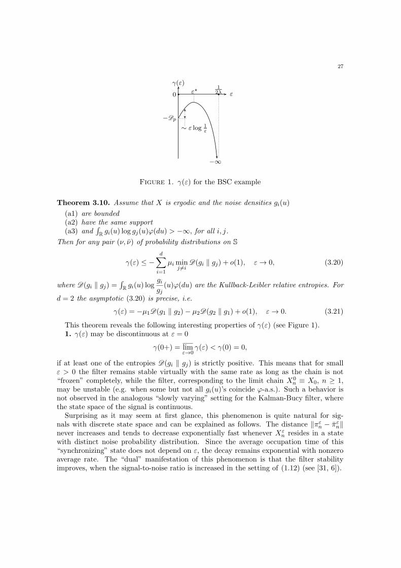
γ(ε)
Figure 1. γ(ε) for the BSC example
Theorem 3.10. Assume that X is ergodic and the noise densities gi(u)
(a1) are bounded(a2) have the same support(a3) and
∫R gi(u) log gj(u)φ(du) > −∞, for all i, j.
Then for any pair (ν, ν) of probability distributions on S
γ(ε) ≤ −d∑
i=1
µiminj =i
D(gi ∥ gj) + o(1), ε→ 0, (3.20)
where D(gi ∥ gj) =∫R gi(u) log
gigj(u)φ(du) are the Kullback-Leibler relative entropies. For
d = 2 the asymptotic (3.20) is precise, i.e.
γ(ε) = −µ1D(g1 ∥ g2)− µ2D(g2 ∥ g1) + o(1), ε→ 0. (3.21)
This theorem reveals the following interesting properties of γ(ε) (see Figure 1).1. γ(ε) may be discontinuous at ε = 0
γ(0+) = limε→0
γ(ε) < γ(0) = 0,
if at least one of the entropies D(gi ∥ gj) is strictly positive. This means that for smallε > 0 the filter remains stable virtually with the same rate as long as the chain is not“frozen” completely, while the filter, corresponding to the limit chain X0
n ≡ X0, n ≥ 1,may be unstable (e.g. when some but not all gi(u)’s coincide φ-a.s.). Such a behavior isnot observed in the analogous “slowly varying” setting for the Kalman-Bucy filter, wherethe state space of the signal is continuous.
Surprising as it may seem at first glance, this phenomenon is quite natural for sig-nals with discrete state space and can be explained as follows. The distance ∥πεn − πεn∥never increases and tends to decrease exponentially fast whenever Xε
n resides in a statewith distinct noise probability distribution. Since the average occupation time of this“synchronizing” state does not depend on ε, the decay remains exponential with nonzeroaverage rate. The “dual” manifestation of this phenomenon is that the filter stabilityimproves, when the signal-to-noise ratio is increased in the setting of (1.12) (see [31, 6]).
28 PAVEL CHIGANSKY
2. As demonstrated in the following example, γ(ε) may have a maximum at someε⋆ > 0 or, in other words, stability may improve when the chain is slowed down! Thisprovides yet another evidence against the false intuition, directly relating stability of thefilter to ergodic properties of the signal (as was explained in the introduction ). The reasonfor such behavior stems from the delicate interplay between two stabilizing mechanisms:ergodicity of the signal and synchronizing effect of the observations. The first dominatesthe second for the faster chain, and vise versa when the chain is slow.
Example 3.11. Consider the so called Binary Symmetric Channel (BSC) model, forwhich Xn ∈ 0, 1 is a symmetric chain with the jump probability λ and Yn = (Xn− ξn)2,where ξ is an i.i.d. 0, 1 binary sequence with P(ξ1 = 1) = p ∈ (0, 1/2). Let Xε andY ε denote the “slow” instances as defined above. In this case more can be said about theconvergence in (3.21) (see the proof below), namely
γ(ε) ≥ −Dp +4λ(log(2)− h(p)
)Dp
ε log ε−1(1 + o(1)
), ε→ 0. (3.22)
where Dp := p logp
1− p+ (1 − p) log
1− p
pand h(p) = −p log p − (1 − p) log(1 − p). On
the other hand, γ(ε) ≤ log(1− 2ελ) → −∞ as ε→ 1/(2λ) (at ε = 1/(2λ) the chain is justan i.i.d. sequence). Since the second term in the expansion of γ(ε) in (3.22) is positiveand by (3.21) γ(ε) → −Dp as ε→ 0, one gets the qualitative behavior depicted in Figure1.
The statement of Theorem 3.10 follows from (3.17) and asymptotic expressions derivedin Lemmas 3.12 and 3.13 below.
3.2.1. Asymptotic expression for λ1(ε).
Lemma 3.12. For any ε > 0 the Markov process (Xε, πε) has a unique stationary invari-ant measure Mε. The top Lyapunov exponent is given by
λ1(ε) =
∫Sd−1
d∑i=1
(Λε∗u
)i
∫Rgi(y) log
∣∣G(y)Λε∗u∣∣φ(dy)Mε
π(du), (3.23)
where Mεπ is the π-marginal of Mε. For each Jj = aℓ : D(gj ∥ gℓ) = 0
limε→0
∫ (1x∈Jj −
∑ℓ:aℓ∈Jj
uℓ)2Mε(dx, du) = 0 (3.24)
and in particular
limε→0
λ1(ε) =
d∑i=1
µi
∫Rgi(y) log gi(y)φ(dy). (3.25)
Proof. Ergodicity of (Xε, πε) essentially follows from the stability (3.10) and was alreadymentioned in Theorem 3.3 above (Corollary 3.5, see also [22]). Concentration propertiesof Mε
π have been studied in [41], when all the noises are distinct, i.e. D(gi ∥ gj) > 0 forall i = j, which is not necessarily the case here.
29
Let Xε be the stationary chain (i.e. X0 ∼ µ) and πε the corresponding optimal filtering
process, generated by (2.1) subject to πε0 = µ. For an f : S → R and n,m ≥ 0 (Y ε denotes
the observations corresponding to Xε)
E(f(Xε
n+m)− πεn+m(f))2
= E(f(Xε
n+m)− E(f(Xε
n+m)∣∣F Y ε
n+m
))2≤
E(f(Xε
n+m)− E(f(Xε
n+m)∣∣F Y ε
[m+1,n+m]
))2 †= E
(f(Xε
n)− E(f(Xε
n)∣∣F Y ε
n
))2=
E(f(Xε
n)− πεn(f))2,
where stationarity of (Xε, Y ε) have been used in †. This means that the filtering errorfor the stationary signal does not increase with time. Then by uniqueness of Mε for anyfixed m ≥ 0∫ (
f(x)− u(f))2Mε(dx, du) =
limn→∞
E(f(Xε
n)− πεn(f))2 ≤ E
(f(Xε
m)− πεm(f))2. (3.26)
Define
πεn(i) =µi∏n
k=1 gi(Yεk )∑d
j=1 µj∏n
k=1 gj(Yεk ), i = 1, ..., d
and let Aεm = Xε
k = X0, ∀k ≤ m, the event that Xεk does not jump on [0,m]. Notice
that on the set Aεm, the observation process is independent of ε, namely
Y εk ≡ Y 0
k =
d∑i=1
1X0=aiξk(i), k = 1, ...,m.
Then by optimality of πε
E(f(Xε
m)− πεm(f))2 ≤ E
(f(Xε
m)− πεm(f))2
=
E1Aεm(f(X0)− π0m(f)
)2+ E1Ω\Aε
m(f(Xε
m)− πεm(f))2 ≤
E(f(X0)− π0m(f)
)2+ 4d2max
ai∈S|f(ai)|2
(1− P(Aε
m))−−−→ε→0
E(f(X0)− π0m(f)
)2For f(x) := 1x∈Jj the latter and (3.26) implies
limε→0
∫ (1x∈Jj −
∑ℓ:aℓ∈Jj
uℓ)2Mε(dx, du) ≤ E
(f(X0)− πm(f)
)2 −−−−→m→∞
0,
where the convergence holds since X0 ∈ Jj ∈ F Y 0
∞ =∨
n≥1 F Y 0
n by definition of Jj and
since π0m(i), i = 1, ..., d are the optimal estimates of 1X0=ai given F Y 0
m .
Once the existence of ergodic stationary pair (Xε, πε) is established21 one may use itto realize the limit λ1 by means of the approach due to H.Furstenberg and R.Khasminskii
21such pair can be generated by taking both X0 and π0 randomly distributed according to Mε and itsdefinition can be extended to the negative times by the usual arguments. Note that this is different from
(Xε, πε) used in the proof of Mε concentration
30 PAVEL CHIGANSKY
(see e.g. [40]). The idea is to study the growth rate of ρεn by projecting it on the unitsphere (Sd−1 in this case):
|ρεn| =∣∣G(Y ε
n )Λε∗ρεn−1
∣∣ = |ρεn−1|∣∣∣G(Y ε
n )Λε∗ ρ
εn−1
|ρεn−1|
∣∣∣ = |ρεn−1|∣∣G(Y ε
n )Λε∗πεn−1
∣∣.Then by the law of large numbers (LLN) for ergodic processes (the required integrabilityconditions are provided by (a1) and (a3))
λ1(ε) = limn→∞
1
nlog |ρεn| = lim
n→∞
1
n
n∑m=1
log∣∣G(Y ε
n )Λε∗πεn−1
∣∣ = E log∣∣G(Y ε
1 )Λε∗πε0
∣∣ =E
d∑i=1
1Xε1=ai log
∣∣G(ξ1(i))Λε∗πε0∣∣ = E
d∑i=1
P(Xε
1 = ai|F Y ε
(−∞,0]
)log∣∣G(ξ1(i))Λε∗πε0
∣∣ =E
d∑i=1
(Λε∗πε0
)ilog∣∣G(ξ1(i))Λε∗πε0
∣∣. (3.27)
The latter expression is nothing but (3.23). The asymptotic (3.25) follows from Λε = I +O(ε) and the concentration (3.24) ofMε as ε→ 0, since gi(u)’s coincide φ-almost surely for
all ai ∈ Jj for any j and the X-marginal of Mε is given by MεX(dx) =
∑di=1 µiδai(dx).
3.2.2. Asymptotic bound for λ1(ε) + λ2(ε).
Lemma 3.13. For any ν, ν ∈ Sd−1
limn→∞
1
nlog |ρεn ∧ ρεn| ≤
d∑i=1
µimaxk =m
∫Rgi(u) log
(gm(u)gk(u)
)φ(du) + o(1), ε→ 0. (3.28)
In the case d = 2
limn→∞
1
nlog |ρεn ∧ ρεn| = log(1− ελ12 − ελ21)+
µ1
∫Rg1(u) log
(g1(u)g2(u)
)φ(du) + µ2
∫Rg2(u) log
(g1(u)g2(u)
)φ(du). (3.29)
Proof. The process Rεn := ρεn ∧ ρεn evolves in the space of antisymmetric matrices (with
zero diagonal) and satisfies the linear equation
Rεn = G(Y ε
n )Λε∗Rε
n−1ΛεG(Y ε
n ), Rε0 = ν ∧ ν,
or in the componentwise notation
Rεn(i, j) =
∑1≤k =ℓ≤d
gk(Yεn )λ
εkiR
εn−1(k, ℓ)λ
εℓjgℓ(Y
εn ), i = j.
Unlike in the case of (3.12), it is not clear whether the limit limn→∞1n log |Rε
n| dependson ν, ν or Πε
n = Rεn/|Rε
n| has any useful concentration properties as ε → 0. However the
31
technique used in the previous section still gives the upper bound. With a fixed integerr ≥ 1
|Rεn| =|Rε
n−r|∣∣∣G(Y ε
n )Λε∗...
G(Y ε
n−r+1)Λε∗Πε
n−rΛεG(Y ε
n−r+1)...ΛεG(Y ε
n )∣∣∣ ≤
|Rεn−r|
(∑i=j
∣∣Πεn−r(i, j)
∣∣ n∏m=n−r+1
gi(Yεm)gj(Y
εm) + c1(r)ε
)≤
|Rεn−r|
(maxi=j
n∏m=n−r+1
gi(Yεm)gj(Y
εm) + c1(r)ε
), n ≥ r
with a constant c1(r) > 0, depending only on r (due to assumption (a1)). By the MET
the limit limn→∞1n log |Rε
n| exists P-a.s and hence (recall the definitions of Y ε and Aεr on
page 29)
limn→∞
1
nlog |Rε
n| = limℓ→∞
1
ℓrlog |Rε
ℓr| ≤
≤ limℓ→∞
1
ℓ
ℓ∑k=1
1
rlog(maxi=j
kr∏m=kr−r+1
gi(Yεm)gj(Y
εm) + c1(r)ε
) †=
1
rE log
(maxi =j
r∏m=1
gi(Yεm)gj(Y
εm) + c1(r)ε
)≤
1
rE1Aε
r log(maxi =j
r∏m=1
gi(Yεm)gj(Y
εm) + c1(r)ε
)+ c2(r)
(1− Pµ(A
εr))≤
1
r
d∑ℓ=1
µℓE log(maxi=j
r∏m=1
gi(ξm(ℓ)
)gj(ξm(ℓ)
)+ c1(r)ε
)+ c3(r)
(1− Pµ(A
εr)) ε→0−−−→
d∑ℓ=1
µℓEmaxi=j
1
rlog
r∏m=1
gi(ξm(ℓ)
)gj(ξm(ℓ)
),
where the LLN was used in † and ci(r) stand for r-dependent constants. Applying theLLN once again one gets for each ℓ
1
rlog
r∏m=1
gi(ξm(ℓ)
)gj(ξm(ℓ)
)=
1
r
r∑m=1
log gi(ξm(ℓ)
)gj(ξm(ℓ)
) r→∞−−−→∫Rgℓ(u) log
(gi(u)gj(u)
)φ(du), P− a.s.
Since “max” is a continuous function
maxi =j
1
rlog
r∏m=1
gi(ξm(ℓ)
)gj(ξm(ℓ)
) r→∞−−−→ maxi=j
∫Rgℓ(u) log
(gi(u)gj(u)
)φ(du)
32 PAVEL CHIGANSKY
and by the uniform integrability, provided by assumption (a3),
Emaxi=j
1
rlog
r∏m=1
gi(ξm(ℓ)
)gj(ξm(ℓ)
) r→∞−−−→ maxi =j
∫Rgℓ(u) log
(gi(u)gj(u)
)φ(du).
Putting all parts together one gets the bound (3.28). In the case d = 2, the processRε
n is one dimensional and all the calculations can be carried out exactly, leading to theexpression (3.29).
3.2.3. Proof of (3.22). When the observation process Y εn takes values in a discrete alphabet
S′ = b1, ..., bd′, the conditional densities (with respect to the point measure φ(dy) =∑d′
i=1 δbi(dy)) are of the form
gi(y) =d′∑j=1
pij1y=bj,d′∑j=1
pij = 1, pij ≥ 0,
and hence by (3.27) (πε1|0 := Λε∗πε0 for brevity)
λ1(ε) = E log∣∣G(Y ε
1 )Λε∗πε0
∣∣ = Ed′∑j=1
1Y ε1 =bj log
( d∑i=1
pijπε1|0(i)
)=
Ed′∑j=1
P(Y ε1 = bj |F Y ε
(−∞,0]
)logP
(Y ε1 = bj |F Y ε
(−∞,0]
)=: −H (Y ε), (3.30)
where H (Y ε) is known as the entropy rate of the stationary process Y ε = (Y εn )n∈Z.
Consider now the special case, when Xε and Y ε take values in S = 0, 1 and p =P(Y ε
n = i|Xεn = j) for i = j. The vector πεn is one dimensional and hence P
(Y ε1 =
1|F Y ε
(−∞,0]
)= (1− p)πε1|0 + p(1− πε1|0), where
πε1|0 := P(Xε
1 = 1|F Y ε
(−∞,0]
)= (1− ελ10)π
ε0 + ελ01(1− πε0) (3.31)
and πε0 := P(Xε0 = 1|F Y ε
(−∞,0]) are redefined for brevity.
Let h(x) := −x log x− (1− x) log(1− x), x ∈ [0, 1] and ℓp(q) = (1− p)q+ p(1− q), anddefine
H(p, q) := h(ℓp(q)
)p, q ∈ [0, 1],
where 0 log 0 ≡ 0 is understood. Since h(x) ≤ log(2) with equality at x = 1/2 andℓp(1/2) = 1/2, H(p, q) ≤ log(2) for all p, q ∈ [0, 1] with equality at q = 1/2. Since h(x) isa concave function, symmetric around x = 1/2
H(p, q) = h((1− p)q + p(1− q)
)≥ qh(1− p) + (1− q)h(p) = h(p), p ∈ [0, 1],
with equality at q = 0 and q = 1. Finally for any fixed p ∈ [0, 1], q 7→ H(p, q) inheritsconcavity and symmetry from h(x). These properties imply the following lower bound
H(p, q) ≥ h(p) +log(2)− h(p)
1/2min(q, 1− q), p, q ∈ [0, 1]. (3.32)
33
By Theorem 1 in [41] for the symmetric chain Xε with jump probability λ and p = 1/2
Emin(πε0, 1− πε0) = P(Xε
0 = argmaxiπε0(i))=
λ
Dpε log ε−1
(1 + o(1)
), ε→ 0, (3.33)
where Dp := p logp
1− p+ (1− p) log
1− p
p. The expression for H (Y ε) in the case d = 2
reads
H (Y ε) = EH(p, πε1|0) = EH(p, πε0) +O(ε), ε→ 0
where the latter asymptotic follows from (3.31), since H(p, q) is differentiable in q.Now (3.32) and (3.33) imply
H (Y ε) ≥ h(p) + 2(log(2)− h(p)
) λDp
ε log ε−1(1 + o(1)
), ε→ 0,
and (3.22) follows from (3.17), (3.29) and (3.30).
Remark 3.14. This Lyapunov exponents approach does not actually require neither er-godicity of the signal nor compactness of the state space. With some sophistication andunder certain structural constraints both cases can be treated - [3], [16], [36].
3.3. Conditional time reversal. As was already mentioned above, the assumption ν ≪ν implies P ≪ P with (recall that we work with coordinate process on the canonical space)
dP
dP(x, y) =
dν
dν(x0), P− a.s.
Consequently PY ≪ PY and PYn ≪ PY
n and
dPYn
dPYn
(Y ) = E(dνdν
(X0)|F Yn
), and
dPY
dPY(Y ) = lim
n→∞
dPYn
dPYn
(Y ) = E(dνdν
(X0)∣∣F Y
[1,∞)
),
where F Y[1,∞) :=
∨n≥1 F Y
n . If in addition, ν ∼ ν, then the above measures are absolutely
continuous as well and the Radon-Nikodym derivatives are positive P-a.s. and P-a.s. Weaccept the latter assumption below for simplicity, though the weaker ν ≪ ν is essentiallyneeded (the reader is referred to [24] for details). When ν ∼ ν, both filtering processes πand π are well defined both on (Ω,F ,P) and (Ω,F , P) as the solutions of (2.1) subject toν and ν respectively. Obviously π is the conditional distribution of Xn given F Y
n underP and the “wrong” filtering under P (obtained by starting (2.1) from ν, while (X,Y )corresponds to ν). Analogously π is the conditional distribution of Xn given F Y
n under Pand is the “wrong” filtering under P. The formula for transformation of the conditionalexpectations under a.c. change of measure from Lemma 2.1 implies
πn(f) = E(f(Xn)|F Y
n
)=
E(f(Xn)
dνdν (X0)
∣∣F Yn
)E(dνdν (X0)
∣∣F Yn
) (3.34)
34 PAVEL CHIGANSKY
for any measurable bounded f . Then
E∣∣πn(f)− πn(f)
∣∣ = EE(dνdν
(X0)∣∣F Y
n
)∣∣πn(f)− πn(f)∣∣ =
E
∣∣∣∣E(dνdν (X0)∣∣F Y
n
)πn(f)− E
(dνdν
(X0)∣∣F Y
n
)E(f(Xn)|F Y
n
)∣∣∣∣ =E
∣∣∣∣E(f(Xn)dν
dν(X0)
∣∣F Yn
)− E
(dνdν
(X0)∣∣F Y
n
)E(f(Xn)|F Y
n
)∣∣∣∣,where the latter equality is due to (3.34). Let |f | ≤ C for definiteness, then the latterimplies 22
E∣∣πn(f)− πn(f)
∣∣ =E
∣∣∣∣E(f(Xn)E(dνdν
(X0)∣∣F Y
n ∨Xn
)∣∣∣F Yn
)− E
(f(Xn)E
(dνdν
(X0)∣∣F Y
n
)∣∣∣F Yn
)∣∣∣∣ ≤E
∣∣∣∣f(Xn)E(dνdν
(X0)∣∣F Y
n ∨Xn
)− f(Xn)E
(dνdν
(X0)∣∣F Y
n
)∣∣∣∣ ≤CE
∣∣∣∣E(dνdν (X0)∣∣F Y
n ∨Xn
)− E
(dνdν
(X0)∣∣F Y
n
)∣∣∣∣.(3.35)
By the Markov property of (X,Y ),
E(dνdν
(X0)∣∣F Y
n ∨Xn
)= E
(dνdν
(X0)∣∣F Y
[1,n] ∨ FX[n,∞)
)= E
(dνdν
(X0)∣∣F Y
[1,∞) ∨ FX[n,∞)
)where FX
[n,∞) := σXn, Xn+1, .... By the martingale convergence theorem23 P-a.s.
limn→∞
E(dνdν
(X0)∣∣F Y
[1,∞) ∨ FX[n,∞)
)= E
(dνdν
(X0)∣∣ ∩n≥0
F Y[1,∞) ∨ FX
[n,∞)
),
limn→∞
E(dνdν
(X0)∣∣F Y
n
)= E
(dνdν
(X0)∣∣F Y
[1,∞)
).
(3.36)
Thus (3.35) implies stability of (2.1) (in the sense limn→∞ E|πn(f) − πn(f)| = 0 for anymeasurable and bounded function f) if∩
n≥0
F Y[1,∞) ∨ FX
[n,∞) = F Y[1,∞), P− a.s. (3.37)
If the tail σ-algebra of X is P-a.s. empty:∩
n≥0 FX[n,∞) = ∅,Ω P-a.s. then the latter is
a particular case of the following question. Let Gn be a decreasing sequence of σ-algebrasand F be a fixed σ-algebra. Is the following true (per se or P-a.s.)∩
n≥0
F ∨ Gn?= F ∨
∩n≥0
Gn. (3.38)
Little is known about the conditions, under which this relation holds, and in fact, accordingto D.Williams [76], it “...trapped up even Kolmogorov and Wiener” (see Sinai [66, p. 837]
22FYn ∨Xn is short for the more proper notation FY
n ∨ σXn23note that the filtration FY
[1,∞) ∨ FX[n,∞) is decreasing with n, while FY
n is increasing, so actually the
direct and reverse martingale convergence theorems are used here
35
for some details). The reader can find a discussion concerning (3.38) in von Weizsacker[75] (note, however, that the counterexample there is incorrect). Other works related tothis issue are [77],[39], [34]. Different counterexamples to (3.38) appeared in Exercise 4.12in Williams [76] and in [62]. In fact Example 1.1 is nothing but another situation when(3.38) fails. F Y
[1,∞) determines all the transitions 1, 3 ↔ 2, 4 of X but does not tell
where Xn resides for each n ≥ 0. Specifying the value of Xn at any n ≥ 0, “pins” thisuncertainty and thus reveals all the information about X. In other words,
F Y[1,∞) ∨ FX
[n,∞) = F Y[1,∞) ∨ FX
[1,∞) + F Y[1,∞)
with strict inclusion. The signal X in this example is an ergodic finite state Markov chainand hence it is geometrically ergodic and its tail σ-algebra is empty, i.e.
∩n≥0 FX
[n,∞) =
∅,Ω. Thus stability of the filter is not implied merely by ergodicity of the signal!The validity of the relation similar to (3.37) was implicitly claimed by H.Kunita in [45](under certain additional technical conditions) and this gap in the proof currently lacksjustification (see [8], [14]).
However (3.35) hints that instead of studying the stability of the conditional distributionof Xn given F Y
n , one may study the time reversed conditional distribution of X0, givenF Y
n ∨Xn. It turns out that the latter has interesting dynamics, somewhat more amenableto stability analysis. The following theorem is taken from [24].
Theorem 3.15. Assume that X is an ergodic chain and ν ∼ ν, then
limn→∞
1
nlog ∥πn − πn∥ ≤ −λ⋄
λ∗, (3.39)
where λ⋄ :=∑d
i=1 µiminj λij.
Remark 3.16. This theorem states that the filter is stable, if Λ is m-primitive and at leastone of its rows has all nonzero entries. The assertion is independent of the observationdensities structure, just like (3.11). Though (3.39) is weaker than (3.11), both are strongerthan just ergodicity of the chain X. This raises the following question: what is thenecessary and sufficient condition for the filtering stability only in terms of the ergodicproperties of the chain, or in other words, what is the weakest ergodic property to beinherited by the filter ?
Proof. Define qn(i, j) := P(X0 = ai|F Yn , Xn = aj). These backward probabilities satisfy
the following recursions (derived via Bayes formulae - see Lemma 3.1, [24]): for eachi = 1, ..., d
qn(i, j) =
∑dℓ=1 λℓjπn−1(ℓ)qn−1(i, ℓ)∑d
ℓ=1 λℓjπn−1(ℓ), n ≥ 1, (3.40)
subject to q0(i, j) := 1i=j. These recursions are linear in q with the time inhomogeneouscoefficients depending on πn. Namely let qn(i) denote the vector with entries qn(i, j),j = 1, ..., d, then
qn(i) = Qn−1qn−1(i), n ≥ 1
where Qn is the matrix with entries
Qn(j, k) =λkjπn(k)∑dℓ=1 λℓjπn(ℓ)
.
36 PAVEL CHIGANSKY
Each row of Qn sums up to 1 and hence Qn is a (random) transition probability matrix.For a fixed i, introduce the upper and lower envelopes of qn(i, j):
qmaxn (i) := max
jqn(i, j), and qmin
n (i) := minjqn(i, j).
Then we have
qn(i, j)− qn(i, j′) =
d∑ℓ=1
Qn−1(j, ℓ)qn−1(i, ℓ)−d∑
ℓ=1
Qn−1(j′, ℓ)qn−1(i, ℓ) =
qmaxn (i)− qmin
n (i)−d∑
ℓ=1
Qn−1(j, ℓ)(qmaxn−1(i)− qn−1(i, ℓ)
)−
d∑ℓ=1
Qn−1(j′, ℓ)(qn−1(i, ℓ)− qmin
n−1(i))
Define ∆n(i) := qmaxn (i)− qmin
n (i) > 0 and αn(i, ℓ) :=qn(i, ℓ)− qmin
n (i)
∆n(i), so that
qn(i, j)−qn(i, j′) = ∆n−1(i)
(1−
d∑ℓ=1
(Qn−1(j, ℓ)
(1−αn−1(i, ℓ)
)+Qn−1(j
′, ℓ)αn−1(i, ℓ)))
≤ ∆n−1(i)(1−
d∑ℓ=1
Qn−1(j, ℓ) ∧Qn−1(j′, ℓ)),
where the latter inequality holds via minimization of the convex sum (recall that αn ∈[0, 1]). Since the latter holds for any j and j′, in particular we have
∆n(i) ≤ ∆n−1(i)(1−
d∑ℓ=1
Qn−1(j, ℓ) ∧Qn−1(j′, ℓ)). (3.41)
Taking a closer look at the expressions in the sum, we obtain
Qn−1(j, ℓ) ∧Qn−1(j′, ℓ) =
λℓjπn(ℓ)∑dℓ=1 λℓjπn(ℓ)
∧ λℓj′πn(ℓ)∑dℓ=1 λℓj′πn(ℓ)
≥(λℓj ∧ λℓj′
)λ∗
πn(ℓ) ≥minj λℓjλ∗
πn(ℓ)
Iterating the latter inequality one gets
maxi,j,k
∣∣qn(i, j)− qn(i, k)∣∣ ≤ max
i∆n(i) ≤
n∏k=1
(1−
d∑ℓ=1
minj λℓjλ∗
πk−1(ℓ)). (3.42)
37
Finally, using the formula (3.34), one gets (qn(i, j) := P(X0 = ai|F Yn , Xn = aj) and
0/0 = 0 is agreed here)
∥πn − πn∥ =d∑
j=1
|πn(j)− πn(j)| =
1
E(dνdν (X0)
∣∣F Yn
) d∑j=1
∣∣∣∣E(1Xn=ajdν
dν(X0)|F Y
n
)− πn(j)E
(dνdν
(X0)∣∣F Y
n
)∣∣∣∣ =1
E(dνdν (X0)
∣∣F Yn
) d∑j=1
∣∣∣∣πn(j) d∑i=1
dν
dν(ai)qn(i, j)− πn(j)
d∑i=1
d∑k=1
dν
dν(ai)qn(i, k)πn(k)
∣∣∣∣ ≤1
E(dνdν (X0)
∣∣F Yn
) d∑j=1
πn(j)d∑
k=1
πn(k)d∑
i=1
dν
dν(ai)
∣∣qn(i, j)− qn(i, k)∣∣ ≤
dmaxi
(νi/νi)maxi
(νi/νi)
n∏k=1
(1−
d∑ℓ=1
minj λℓjλ∗
πk−1(ℓ)).
This implies (3.39):
limn→∞
1
nlog ∥πn − πn∥ = lim
n→∞
1
n
n∑k=1
log(1−
d∑ℓ=1
minj λℓjλ∗
πk−1(ℓ))≤
−d∑
ℓ=1
minj λℓjλ∗
limn→∞
1
n
n∑k=1
πk−1(ℓ)
where the latter inequality holds P-a.s. (and thus also P-a.s.) by the law of large numbersfor the filtering process πn, which is the exact conditional distribution under P. Indeed
πn = Λ∗πn−1 +Mn,
where Mn := πn − Λ∗πn−1 are bounded martingale differences under P. Hence
1
n
n∑m=1
Mm = 0
(Theorem 4. Ch. VII, Section 5 in [64]). Since 1n
∑nk=1 πk ∈ Sd−1 and by ergodicity of X,
the equation x = Λ∗x has a unique root in Sd−1, i.e. x := µ, the limit 1n
∑nk=1 πk exists
and equals µ. Similar result holds in the general setting, as in Theorem 3.6
Theorem 3.17 (Theorem 1.1 in [24]). Let µ(x) be the unique invariant density of X andassume that λ⋄ :=
∫S ess infu∈S λ(x, u)µ(x)ψ(dx) > 0 and λ(x, u) ≤ λ∗ < ∞. Then for
any initial densities ν(x) and ν(x) ≥ ν∗ > 0
limn→∞
1
nlog ∥πn − πn∥ ≤ −λ⋄/λ∗, P− a.s.
38 PAVEL CHIGANSKY
References
1. Oseledec’s multiplicative ergodic theorem: a proof, Random matrices and their applications (Brunswick,Maine, 1984), Contemp. Math., vol. 50, Amer. Math. Soc., Providence, RI, 1986, pp. 23–30.MR MR841079 (87k:60029)
2. Ludwig Arnold, Random dynamical systems, Springer Monographs in Mathematics, Springer-Verlag,Berlin, 1998. MR MR1723992 (2000m:37087)
3. Rami Atar, Exponential stability for nonlinear filtering of diffusion processes in a noncompact domain,Ann. Probab. 26 (1998), no. 4, 1552–1574. MR MR1675039 (99k:93088)
4. Rami Atar, Frederi Viens, and Ofer Zeitouni, Robustness of Zakai’s equation via Feynman-Kac repre-sentations, Stochastic analysis, control, optimization and applications, Systems Control Found. Appl.,Birkhauser Boston, Boston, MA, 1999, pp. 339–352. MR MR1702969 (2000f:93086)
5. Rami Atar and Ofer Zeitouni, Exponential stability for nonlinear filtering, Ann. Inst. H. PoincareProbab. Statist. 33 (1997), no. 6, 697–725. MR MR1484538 (98i:60070)
6. , Lyapunov exponents for finite state nonlinear filtering, SIAM J. Control Optim. 35 (1997),no. 1, 36–55. MR MR1430282 (97k:93065)
7. , A note on the memory length of optimal nonlinear filters, Systems Control Lett. 35 (1998),no. 2, 131–135. MR MR1654897 (99j:93100)
8. Peter Baxendale, Pavel Chigansky, and Robert Liptser, Asymptotic stability of the Wonham filter:ergodic and nonergodic signals, SIAM J. Control Optim. 43 (2004), no. 2, 643–669 (electronic).MR 2086177 (2005e:93152)
9. A. G. Bhatt, A. Budhiraja, and R. L. Karandikar, Markov property and ergodicity of the nonlinearfilter, SIAM J. Control Optim. 39 (2000), no. 3, 928–949 (electronic). MR MR1786337 (2001m:93122)
10. Garrett Birkhoff, Lattice theory, Third edition. American Mathematical Society Colloquium Publica-tions, Vol. XXV, American Mathematical Society, Providence, R.I., 1967. MR MR0227053 (37 #2638)
11. David Blackwell, The entropy of functions of finite-state Markov chains, Transactions of the firstPrague conference on information theory, Statistical decision functions, random processes held atLiblice near Prague from November 28 to 30, 1956, Publishing House of the Czechoslovak Academy ofSciences, Prague, 1957, pp. 13–20. MR MR0100297 (20 #6730)
12. A. Budhiraja, Ergodic properties of the nonlinear filter, Stochastic Process. Appl. 95 (2001), no. 1,1–24. MR MR1847089 (2002e:60065)
13. , On invariant measures of discrete time filters in the correlated signal-noise case, Ann. Appl.Probab. 12 (2002), no. 3, 1096–1113. MR MR1925453 (2003h:60057)
14. , Asymptotic stability, ergodicity and other asymptotic properties of the nonlinear filter, Ann.Inst. H. Poincare Probab. Statist. 39 (2003), no. 6, 919–941. MR MR2010391 (2004h:60063)
15. A. Budhiraja and D. Ocone, Exponential stability of discrete-time filters for bounded observation noise,Systems Control Lett. 30 (1997), no. 4, 185–193. MR MR1455877 (98c:93110)
16. , Exponential stability in discrete-time filtering for non-ergodic signals, Stochastic Process. Appl.82 (1999), no. 2, 245–257. MR MR1700008 (2000d:94010)
17. Amarjit Budhiraja and Harold J. Kushner, Robustness of nonlinear filters over the infinite time inter-val, SIAM J. Control Optim. 36 (1998), no. 5, 1618–1637 (electronic). MR MR1626884 (99f:93133)
18. , Approximation and limit results for nonlinear filters over an infinite time interval, SIAM J.Control Optim. 37 (1999), no. 6, 1946–1979 (electronic). MR MR1720146 (2000i:93080)
19. , Approximation and limit results for nonlinear filters over an infinite time interval. II.Random sampling algorithms, SIAM J. Control Optim. 38 (2000), no. 6, 1874–1908 (electronic).MR MR1776660 (2001f:93070)
20. , Monte Carlo algorithms and asymptotic problems in nonlinear filtering, Stochastics in fi-nite and infinite dimensions, Trends Math., Birkhauser Boston, Boston, MA, 2001, pp. 59–87.MR MR1797081 (2001i:93120)
21. Frederic Cerou, Long time behavior for some dynamical noise free nonlinear filtering problems, SIAMJ. Control Optim. 38 (2000), no. 4, 1086–1101 (electronic). MR MR1760061 (2001c:93096)
22. Pavel Chigansky, An ergodic theorem for filtering with applications to stability, to appear in Systemand Control Letters, 2006.
39
23. , Stability of the nonlinear filter for slowly switching markov chains, Stochastic Process. Appl.116 (2006), no. 8, 1185–1194.
24. Pavel Chigansky and Robert Liptser, Stability of nonlinear filters in nonmixing case, Ann. Appl.Probab. 14 (2004), no. 4, 2038–2056. MR MR2099662 (2005h:62265)
25. , On a role of predictor in the filtering stability, Electronic Comm. Prob. 11 (2006), 129–140.26. Pavel Chigansky and Ramon van Handel, Model robustness of finite state nonlinear filtering over the
infinite time horizon, submitted, 2006.27. J. M. C. Clark, D. L. Ocone, and C. Coumarbatch, Relative entropy and error bounds for filtering
of Markov processes, Math. Control Signals Systems 12 (1999), no. 4, 346–360. MR MR1728373(2001m:60095)
28. Giuseppe Da Prato, Marco Fuhrman, and Paul Malliavin, Asymptotic ergodicity of the process ofconditional law in some problem of non-linear filtering, J. Funct. Anal. 164 (1999), no. 2, 356–377.MR MR1695555 (2000e:93070)
29. Pierre Del Moral and Alice Guionnet, On the stability of interacting processes with applications tofiltering and genetic algorithms, Ann. Inst. H. Poincare Probab. Statist. 37 (2001), no. 2, 155–194.MR MR1819122 (2002k:60013)
30. Pierre Del Moral and Laurent Miclo, On the stability of nonlinear Feynman-Kac semigroups, Ann.Fac. Sci. Toulouse Math. (6) 11 (2002), no. 2, 135–175. MR MR1988460 (2004d:47081)
31. Bernard Delyon and Ofer Zeitouni, Lyapunov exponents for filtering problems, Applied stochasticanalysis (London, 1989), Stochastics Monogr., vol. 5, Gordon and Breach, New York, 1991, pp. 511–521. MR MR1108433 (92i:93092)
32. Giovanni B. Di Masi and Lukasz Stettner, Ergodicity of hidden Markov models, Math. Control SignalsSystems 17 (2005), no. 4, 269–296. MR MR2177319
33. Robert J. Elliott, Lakhdar Aggoun, and John B. Moore, Hidden Markov models, Applications of Mathe-matics (New York), vol. 29, Springer-Verlag, New York, 1995, Estimation and control. MR MR1323178(96h:93001)
34. M. Emery and W. Schachermayer, On Vershik’s standardness criterion and Tsirelson’s notion of cosi-ness, Seminaire de Probabilites, XXXV, Lecture Notes in Math., vol. 1755, Springer, Berlin, 2001,pp. 265–305. MR MR1837293 (2002i:60071)
35. Eberhard Hopf, An inequality for positive linear integral operators, J. Math. Mech. 12 (1963), 683–692.MR MR0165325 (29 #2614)
36. Ze-Chun Hu and Wei Sun, A note on exponential stability of the nonlinear filter for denumerablemarkov chains, to appear in Systems & Control Letters, 2006.
37. Thomas Kaijser, A limit theorem for partially observed Markov chains, Ann. Probability 3 (1975),no. 4, 677–696. MR MR0383536 (52 #4417)
38. Gopinath Kallianpur, Stochastic filtering theory, Applications of Mathematics, vol. 13, Springer-Verlag,New York, 1980. MR MR583435 (82f:60089)
39. Brunon Kaminski, Decreasing nets of σ-algebras and their applications to ergodic theory, Tohoku Math.J. (2) 43 (1991), no. 2, 263–274. MR MR1104432 (92g:28034)
40. R. Z. Khasminskii, Stochastic stability of differential equations, Monographs and Textbooks on Me-chanics of Solids and Fluids: Mechanics and Analysis, vol. 7, Sijthoff & Noordhoff, Alphen aan denRijn, 1980, Translated from the Russian by D. Louvish. MR MR600653 (82b:60064)
41. Rafail Khasminskii and Ofer Zeitouni, Asymptotic filtering for finite state Markov chains, StochasticProcess. Appl. 63 (1996), no. 1, 1–10. MR MR1411186 (97f:93046)
42. Marina Kleptsyna and Alexander Veretennikov, On continuous time ergodic filters with wrong initialdata, available at http://www.univ-lemans.fr/sciences/statist/download/Kleptsyna, 2006.
43. , On discrete time ergodic filters with wrong initial data, available at http://www.univ
-lemans.fr/sciences/statist/download/Kleptsyna, 2006.44. Fred Kochman and Jim Reeds, A simple proof of kaijser’s unique ergodicity result for hidden markov
α-chains, to appear in Annals of Applied Probability, 2006.45. Hiroshi Kunita, Asymptotic behavior of the nonlinear filtering errors of Markov processes, J. Multi-
variate Anal. 1 (1971), 365–393. MR MR0301812 (46 #967)
40 PAVEL CHIGANSKY
46. , Ergodic properties of nonlinear filtering processes, Spatial stochastic processes, Progr. Probab.,vol. 19, Birkhauser Boston, Boston, MA, 1991, pp. 233–256. MR MR1144099 (92m:60062)
47. Harold J. Kushner and Amarjit S. Budhiraja, A nonlinear filtering algorithm based on an approx-imation of the conditional distribution, IEEE Trans. Automat. Control 45 (2000), no. 3, 580–585.MR MR1762882 (2001c:93101)
48. Huibert Kwakernaak and Raphael Sivan, Linear optimal control systems, Wiley-Interscience [JohnWiley & Sons], New York, 1972. MR MR0406607 (53 #10394)
49. Alain Le Breton and Marie-Christine Roubaud, Asymptotic optimality of approximate filters in sto-chastic systems with colored noises, SIAM J. Control Optim. 39 (2000), no. 3, 917–927 (electronic).MR MR1786336 (2001h:93093)
50. Francois Le Gland and Laurent Mevel, Basic properties of the projective product with application toproducts of column-allowable nonnegative matrices, Math. Control Signals Systems 13 (2000), no. 1,41–62. MR MR1742139 (2001b:15033)
51. , Exponential forgetting and geometric ergodicity in hidden Markov models, Math. Control Sig-nals Systems 13 (2000), no. 1, 63–93. MR MR1742140 (2001b:93075)
52. Francois Le Gland and Nadia Oudjane, Stability and uniform approximation of nonlinear filters usingthe Hilbert metric and application to particle filters, Ann. Appl. Probab. 14 (2004), no. 1, 144–187.MR MR2023019 (2004k:62219)
53. Francois LeGland and Nadia Oudjane, A robustification approach to stability and to uniform particleapproximation of nonlinear filters: the example of pseudo-mixing signals, Stochastic Process. Appl.106 (2003), no. 2, 279–316. MR MR1989630 (2004i:93184)
54. Robert S. Liptser and Albert N. Shiryaev, Statistics of random processes. I, expanded ed., Applicationsof Mathematics (New York), vol. 5, Springer-Verlag, Berlin, 2001, General theory, Translated from the1974 Russian original by A. B. Aries, Stochastic Modelling and Applied Probability. MR MR1800857(2001k:60001a)
55. , Statistics of random processes. II, expanded ed., Applications of Mathematics (New York),vol. 6, Springer-Verlag, Berlin, 2001, Applications, Translated from the 1974 Russian original by A. B.Aries, Stochastic Modelling and Applied Probability. MR MR1800858 (2001k:60001b)
56. Armand M. Makowski, Filtering formulae for partially observed linear systems with non-Gaussianinitial conditions, Stochastics 16 (1986), no. 1-2, 1–24. MR MR834558 (87d:93094)
57. D. L. Ocone, Asymptotic stability of Benes filters, Stochastic Anal. Appl. 17 (1999), no. 6, 1053–1074.MR MR1721933 (2001a:60050)
58. Daniel Ocone, Entropy inequalities and entropy dynamics in nonlinear filtering of diffusion processes,Stochastic analysis, control, optimization and applications, Systems Control Found. Appl., BirkhauserBoston, Boston, MA, 1999, pp. 477–496. MR MR1702976 (2000f:93091)
59. Daniel Ocone and Etienne Pardoux, Asymptotic stability of the optimal filter with respect to its initialcondition, SIAM J. Control Optim. 34 (1996), no. 1, 226–243. MR MR1372912 (97e:60073)
60. Nadia Oudjane and Sylvain Rubenthaler, Stability and uniform particle approximation of nonlinearfilters in case of non ergodic signals, Stoch. Anal. Appl. 23 (2005), no. 3, 421–448. MR MR2140972(2005m:93153)
61. Anastasia Papavasiliou, Parameter estimation and asymptotic stability in stochastic filtering, StochasticProcess. Appl. 116 (2006), no. 7, 1048–1065.
62. L. C. G. Rogers, Coupling and the tail σ-field of a one-dimensional diffusion, Stochastic calculus inapplication (Cambridge, 1987), Pitman Res. Notes Math. Ser., vol. 197, Longman Sci. Tech., Harlow,1988, pp. 78–88. MR MR995472 (90f:60142)
63. E. Seneta, Non-negative matrices and Markov chains, Springer Series in Statistics, Springer, NewYork, 2006, Revised reprint of the second (1981) edition [Springer-Verlag, New York; MR0719544].MR MR2209438
64. A. N. Shiryaev, Probability, second ed., Graduate Texts in Mathematics, vol. 95, Springer-Verlag,New York, 1996, Translated from the first (1980) Russian edition by R. P. Boas. MR MR1368405(97c:60003)
65. Louis Shue, Brian D.O. Anderson, and Subhrakanti Dey, Exponential stability of filters and smoothersfor hidden markov models, IEEE Trans. Sig. Proc. 46 (1998), no. 8, 2180–2194.
41
66. Ya. G. Sinaı, Kolmogorov’s work on ergodic theory, Ann. Probab. 17 (1989), no. 3, 833–839.MR MR1009437 (91e:01017)
67. Richard B. Sowers and Armand M. Makowski, Discrete-time filtering for linear systems in correlatednoise with non-Gaussian initial conditions: formulas and asymptotics, Robust control of linear systemsand nonlinear control (Amsterdam, 1989), Progr. Systems Control Theory, vol. 4, Birkhauser Boston,Boston, MA, 1990, pp. 407–419. MR MR1115412 (92i:93096)
68. , Discrete-time filtering for linear systems with non-Gaussian initial conditions: asymptoticbehavior of the difference between the MMSE and LMSE estimates, IEEE Trans. Automat. Control 37(1992), no. 1, 114–120. MR MR1139622 (92j:93130)
69. Wilhelm Stannat, Stability of the filter equation for a time-dependent signal on Rd, Appl. Math. Optim.52 (2005), no. 1, 39–71. MR MR2141176
70. , Stability of the optimal filter via pointwise gradient estimates, available http://www.math.
uni-bielefeld.de/~stannat/, 2006.71. , Stability of the pathwise filter equation on Rd, available at http://www.math.uni-bielefeld.
de/~stannat/, 2006.72. L. Stettner, Invariant measures of the pair: state, approximate filtering process, Colloq. Math. 62
(1991), no. 2, 347–351. MR MR1142935 (93a:60066)73. Lukasz Stettner, On invariant measures of filtering processes, Stochastic differential systems (Bad
Honnef, 1988), Lecture Notes in Control and Inform. Sci., vol. 126, Springer, Berlin, 1989, pp. 279–292. MR MR1236074
74. Vladislav B. Tadic and Arnaud Doucet, Exponential forgetting and geometric ergodicity for opti-mal filtering in general state-space models, Stochastic Process. Appl. 115 (2005), no. 8, 1408–1436.MR MR2152381 (2006f:62094)
75. Heinrich von Weizsacker, Exchanging the order of taking suprema and countable intersections of σ-algebras, Ann. Inst. H. Poincare Sect. B (N.S.) 19 (1983), no. 1, 91–100. MR MR699981 (85c:28001)
76. David Williams, Probability with martingales, Cambridge Mathematical Textbooks, Cambridge Uni-versity Press, Cambridge, 1991. MR MR1155402 (93d:60002)
77. Marc Yor, Tsirelson’s equation in discrete time, Probab. Theory Related Fields 91 (1992), no. 2,135–152. MR MR1147613 (93d:60104)
Department of Mathematics, The Weizmann Institute of Science, Rehovot 76100, IsraelE-mail address: [email protected]