STA 6857—Exploratory Data Analysis & Smoothing inTime Series (§2.3 cont., 2.4)

Exploratory Data Analysis Smoothing in Time Series Homework 2d

Outline

1 Exploratory Data Analysis

2 Smoothing in Time Series

3 Homework 2d

Arthur Berg STA 6857—Exploratory Data Analysis & Smoothing in Time Series (§2.3 cont., 2.4) 2/ 26

Exploratory Data Analysis Smoothing in Time Series Homework 2d

Outline

1 Exploratory Data Analysis

2 Smoothing in Time Series

3 Homework 2d

Arthur Berg STA 6857—Exploratory Data Analysis & Smoothing in Time Series (§2.3 cont., 2.4) 3/ 26

Exploratory Data Analysis Smoothing in Time Series Homework 2d

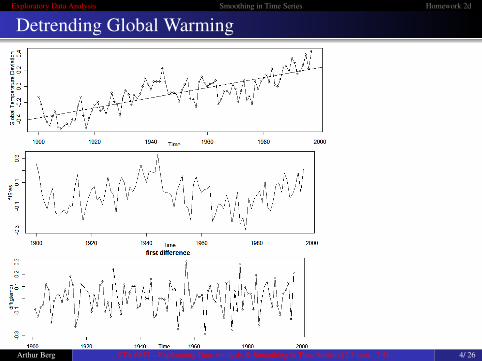
Detrending Global Warming

Arthur Berg STA 6857—Exploratory Data Analysis & Smoothing in Time Series (§2.3 cont., 2.4) 4/ 26

Exploratory Data Analysis Smoothing in Time Series Homework 2d

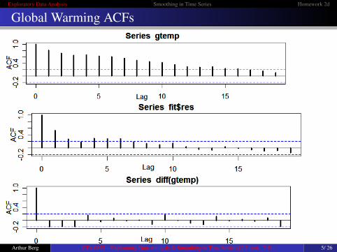
Global Warming ACFs

Arthur Berg STA 6857—Exploratory Data Analysis & Smoothing in Time Series (§2.3 cont., 2.4) 5/ 26

Exploratory Data Analysis Smoothing in Time Series Homework 2d

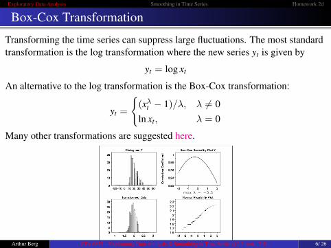
Box-Cox Transformation

Transforming the time series can suppress large fluctuations. The most standardtransformation is the log transformation where the new series yt is given by

yt = log xt

An alternative to the log transformation is the Box-Cox transformation:

yt =

{(xλ

t − 1)/λ, λ 6= 0ln xt, λ = 0

Many other transformations are suggested here.

Arthur Berg STA 6857—Exploratory Data Analysis & Smoothing in Time Series (§2.3 cont., 2.4) 6/ 26

Exploratory Data Analysis Smoothing in Time Series Homework 2d

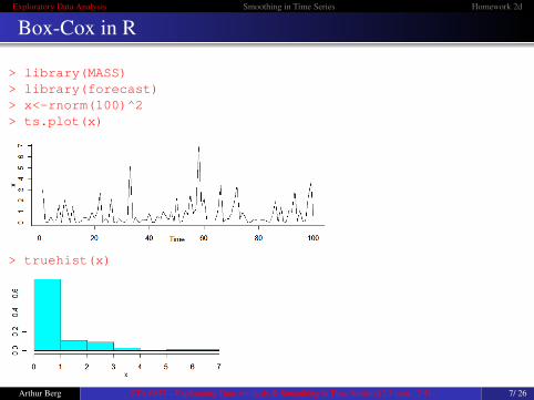
Box-Cox in R

> library(MASS)> library(forecast)> x<-rnorm(100)^2> ts.plot(x)

> truehist(x)

Arthur Berg STA 6857—Exploratory Data Analysis & Smoothing in Time Series (§2.3 cont., 2.4) 7/ 26

Exploratory Data Analysis Smoothing in Time Series Homework 2d

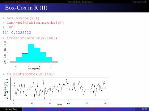
Box-Cox in R (II)

> bc<-boxcox(x~1)> lam<-bc$x[which.max(bc$y)]> lam

[1] 0.2222222

> truehist(BoxCox(x,lam))

> ts.plot(BoxCox(x,lam))

Arthur Berg STA 6857—Exploratory Data Analysis & Smoothing in Time Series (§2.3 cont., 2.4) 8/ 26

Exploratory Data Analysis Smoothing in Time Series Homework 2d

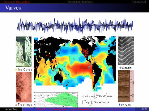
Varves

Arthur Berg STA 6857—Exploratory Data Analysis & Smoothing in Time Series (§2.3 cont., 2.4) 9/ 26

Exploratory Data Analysis Smoothing in Time Series Homework 2d

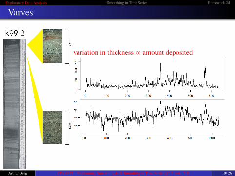
Varves

variation in thickness ∝ amount deposited

Arthur Berg STA 6857—Exploratory Data Analysis & Smoothing in Time Series (§2.3 cont., 2.4) 10/ 26

Exploratory Data Analysis Smoothing in Time Series Homework 2d

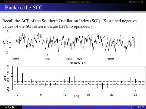
Back to the SOI

Recall the ACF of the Southern Oscillation Index (SOI). (Sustained negativevalues of the SOI often indicate El Niño episodes.)

Arthur Berg STA 6857—Exploratory Data Analysis & Smoothing in Time Series (§2.3 cont., 2.4) 11/ 26

Exploratory Data Analysis Smoothing in Time Series Homework 2d

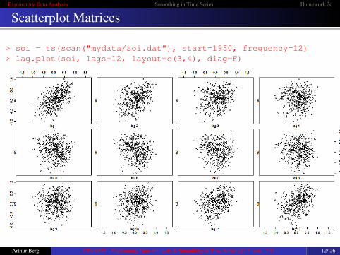
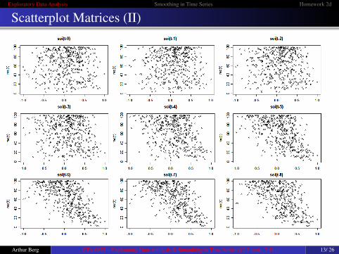
Scatterplot Matrices

> soi = ts(scan("mydata/soi.dat"), start=1950, frequency=12)> lag.plot(soi, lags=12, layout=c(3,4), diag=F)

Arthur Berg STA 6857—Exploratory Data Analysis & Smoothing in Time Series (§2.3 cont., 2.4) 12/ 26

Exploratory Data Analysis Smoothing in Time Series Homework 2d

Scatterplot Matrices (II)

Arthur Berg STA 6857—Exploratory Data Analysis & Smoothing in Time Series (§2.3 cont., 2.4) 13/ 26

Exploratory Data Analysis Smoothing in Time Series Homework 2d

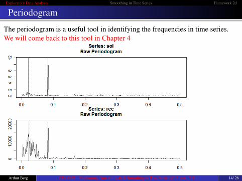
Periodogram

The periodogram is a useful tool in identifying the frequencies in time series.We will come back to this tool in Chapter 4

Arthur Berg STA 6857—Exploratory Data Analysis & Smoothing in Time Series (§2.3 cont., 2.4) 14/ 26

Exploratory Data Analysis Smoothing in Time Series Homework 2d

Outline

1 Exploratory Data Analysis

2 Smoothing in Time Series

3 Homework 2d

Arthur Berg STA 6857—Exploratory Data Analysis & Smoothing in Time Series (§2.3 cont., 2.4) 15/ 26

Exploratory Data Analysis Smoothing in Time Series Homework 2d

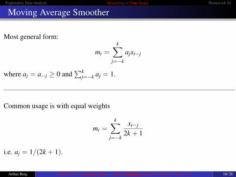
Moving Average Smoother

Most general form:

mt =k∑

j=−k

ajxt−j

where aj = a−j ≥ 0 and∑k

j=−k aj = 1.

Common usage is with equal weights

mt =k∑

j=−k

xt−j

2k + 1

i.e. aj = 1/(2k + 1).

Arthur Berg STA 6857—Exploratory Data Analysis & Smoothing in Time Series (§2.3 cont., 2.4) 16/ 26

Exploratory Data Analysis Smoothing in Time Series Homework 2d

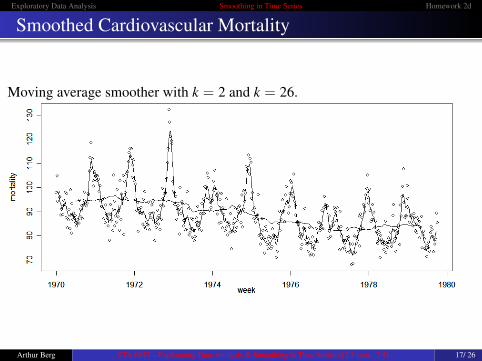
Smoothed Cardiovascular Mortality

Moving average smoother with k = 2 and k = 26.

Arthur Berg STA 6857—Exploratory Data Analysis & Smoothing in Time Series (§2.3 cont., 2.4) 17/ 26

Exploratory Data Analysis Smoothing in Time Series Homework 2d

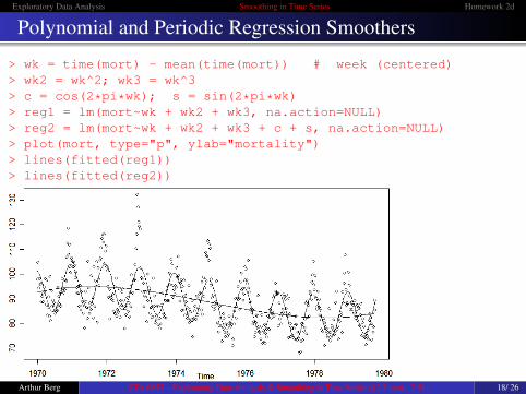
Polynomial and Periodic Regression Smoothers

> wk = time(mort) - mean(time(mort)) # week (centered)> wk2 = wk^2; wk3 = wk^3> c = cos(2*pi*wk); s = sin(2*pi*wk)> reg1 = lm(mort~wk + wk2 + wk3, na.action=NULL)> reg2 = lm(mort~wk + wk2 + wk3 + c + s, na.action=NULL)> plot(mort, type="p", ylab="mortality")> lines(fitted(reg1))> lines(fitted(reg2))

Arthur Berg STA 6857—Exploratory Data Analysis & Smoothing in Time Series (§2.3 cont., 2.4) 18/ 26

Exploratory Data Analysis Smoothing in Time Series Homework 2d

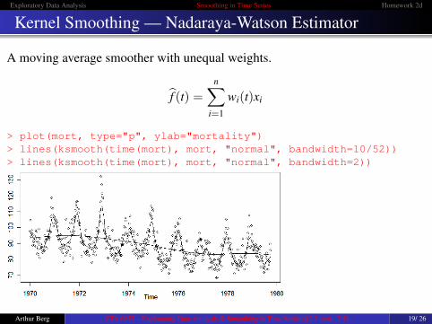
Kernel Smoothing — Nadaraya-Watson Estimator

A moving average smoother with unequal weights.

f̂ (t) =n∑

i=1

wi(t)xi

> plot(mort, type="p", ylab="mortality")> lines(ksmooth(time(mort), mort, "normal", bandwidth=10/52))> lines(ksmooth(time(mort), mort, "normal", bandwidth=2))

Arthur Berg STA 6857—Exploratory Data Analysis & Smoothing in Time Series (§2.3 cont., 2.4) 19/ 26

Exploratory Data Analysis Smoothing in Time Series Homework 2d

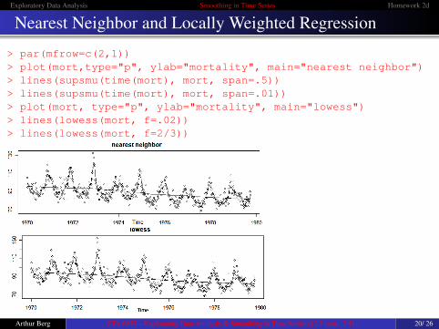
Nearest Neighbor and Locally Weighted Regression

> par(mfrow=c(2,1))> plot(mort,type="p", ylab="mortality", main="nearest neighbor")> lines(supsmu(time(mort), mort, span=.5))> lines(supsmu(time(mort), mort, span=.01))> plot(mort, type="p", ylab="mortality", main="lowess")> lines(lowess(mort, f=.02))> lines(lowess(mort, f=2/3))

Arthur Berg STA 6857—Exploratory Data Analysis & Smoothing in Time Series (§2.3 cont., 2.4) 20/ 26

Exploratory Data Analysis Smoothing in Time Series Homework 2d

Smoothing Splines

> plot(mort, type="p", ylab="mortality")> lines(smooth.spline(time(mort), mort))> lines(smooth.spline(time(mort), mort, spar=1))

Arthur Berg STA 6857—Exploratory Data Analysis & Smoothing in Time Series (§2.3 cont., 2.4) 21/ 26

Exploratory Data Analysis Smoothing in Time Series Homework 2d

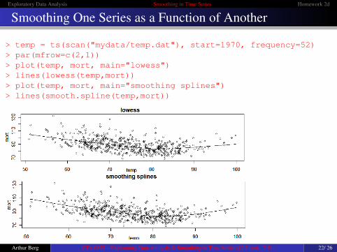
Smoothing One Series as a Function of Another

> temp = ts(scan("mydata/temp.dat"), start=1970, frequency=52)> par(mfrow=c(2,1))> plot(temp, mort, main="lowess")> lines(lowess(temp,mort))> plot(temp, mort, main="smoothing splines")> lines(smooth.spline(temp,mort))

Arthur Berg STA 6857—Exploratory Data Analysis & Smoothing in Time Series (§2.3 cont., 2.4) 22/ 26

Exploratory Data Analysis Smoothing in Time Series Homework 2d

Words of Caution

Much of the theory of these methods applies to IID data and does not takeinto account serial correlation that is typically present in time series.

Different smoothing parameters may give vastly different results.

Arthur Berg STA 6857—Exploratory Data Analysis & Smoothing in Time Series (§2.3 cont., 2.4) 23/ 26

Exploratory Data Analysis Smoothing in Time Series Homework 2d

Outline

1 Exploratory Data Analysis

2 Smoothing in Time Series

3 Homework 2d

Arthur Berg STA 6857—Exploratory Data Analysis & Smoothing in Time Series (§2.3 cont., 2.4) 24/ 26

Exploratory Data Analysis Smoothing in Time Series Homework 2d

Textbook Reading

Read the following sections from the textbookReview Chapter 2

Arthur Berg STA 6857—Exploratory Data Analysis & Smoothing in Time Series (§2.3 cont., 2.4) 25/ 26

Exploratory Data Analysis Smoothing in Time Series Homework 2d

Textbook Problems

Do the following exercise from the textbook2.12

Arthur Berg STA 6857—Exploratory Data Analysis & Smoothing in Time Series (§2.3 cont., 2.4) 26/ 26