This content has been downloaded from IOPscience. Please scroll down to see the full text.

Download details:

IP Address: 138.234.74.104

This content was downloaded on 23/01/2015 at 17:37

Please note that terms and conditions apply.

Spin-dependent macroscopic forces from new particle exchange

View the table of contents for this issue, or go to the journal homepage for more

JHEP11(2006)005

(http://iopscience.iop.org/1126-6708/2006/11/005)

Home Search Collections Journals About Contact us My IOPscience

JHEP11(2006)005

Published by Institute of Physics Publishing for SISSA

Received: June 14, 2006

Revised: September 17, 2006

Accepted: October 17, 2006

Published: November 3, 2006

Spin-dependent macroscopic forces from new particle

exchange

Bogdan A. Dobrescu

Theoretical Physics Department, Fermilab

Batavia, IL 60510, U.S.A.

E-mail: bdob@fnal.gov

Irina Mocioiu

Pennsylvania State University, University Park

PA 16802, U.S.A.

E-mail: irina@phys.psu.edu

Abstract: Long-range forces between macroscopic objects are mediated by light particles

that interact with the electrons or nucleons, and include spin-dependent static compo-

nents as well as spin- and velocity-dependent components. We parametrize the long-range

potential between two fermions assuming rotational invariance, and find 16 different com-

ponents. Applying this result to electrically neutral objects, we show that the macroscopic

potential depends on 72 measurable parameters. We then derive the potential induced

by the exchange of a new gauge boson or spinless particle, and compare the limits set by

measurements of macroscopic forces to the astrophysical limits on the couplings of these

particles.

Keywords: Beyond Standard Model, Cosmology of Theories beyond the SM.

c© SISSA 2006 http://jhep.sissa.it/archive/papers/jhep112006005/jhep112006005.pdf

JHEP11(2006)005

Contents

1. Introduction 1

2. Long-range fermion-fermion interactions in momentum space 2

3. Long-range potentials between fermions 5

4. Interactions between macroscopic objects 7

4.1 Exchange of one boson with standard propagator 8

4.2 Non-standard dispersion relations 11

5. Spin-1 exchange forces 12

5.1 New massless gauge boson 13

5.2 General spin-1 exchange 16

6. Spin-0 exchange forces 21

7. Conclusions 23

A. Vector identities 24

B. Fourier transforms 25

1. Introduction

The electromagnetic and gravitational interactions, mediated by spin-1 and spin-2 parti-

cles, are the only macroscopic forces observed so far. However, other macroscopic forces

could exist, and more sensitive measurements might reveal them. Searches for long-range

spin-independent forces have a long history of substantial improvements achieved by vari-

ous groups (for recent reviews see ref. [1, 2]). By contrast, long-range spin-dependent forces

could lead to a broader variety of observable effects, but so far they have been less intensely

investigated. Most searches have been concentrated on two types of spin-dependent long-

range forces that could be induced by axion exchange, the so-called dipole-dipole and

monopole-dipole interactions [3].

Measurements of forces between macroscopic polarized objects have set limits on

new dipole-dipole potentials among electrons [4 – 8], and between electrons and nucle-

ons [5, 7]. There are also limits on monopole-dipole forces between polarized electrons

and unpolarized objects [5, 9 – 11], as well as between polarized nucleons and unpolarized

objects [5, 9, 12, 13]. Earlier experiments are reviewed in [5, 7, 14, 15].

– 1 –

JHEP11(2006)005

Here we study spin-dependent forces between macroscopic objects that could exist

given general assumptions within quantum field theory. We focus on rotational-invariant

potentials that could be induced by the exchange of new light particles, showing that sev-

eral new kinds of spin-dependent macroscopic forces may exist and should be searched for

in experiments.

The discovery of a new force with a range longer than about a micrometer would

have a tremendous impact on our understanding of nature. Furthermore, even if new

macroscopic forces will not be discovered, setting limits on the various potentials is im-

portant for constraining many extensions of the Standard Model of particle physics. The

spontaneous breaking of continuous symmetries leads to the existence of massless or very

light (pseudo) Nambu-Goldstone bosons, such as axions, familons, majorons, etc. [16].

It is also possible that new massless gauge bosons associated with unbroken gauge sym-

metries exist [17]. Such particles have naturally suppressed interactions with ordinary

matter, but nevertheless could mediate long-range forces that may be accessible to labo-

ratory experiments. As an application, we derive the limits on the couplings of a new

massless spin-1 particle (“paraphoton”) from existing measurements of spin-dependent

forces.

Massive spin-1 particles with general couplings, or bosons of spin-2 or higher, could

also be light enough to mediate macroscopic forces, albeit their low mass and feeble inter-

actions would require very small dimensionless parameters or fine tuning. We will show

that the majority of the rotational-invariant spin-dependent potentials are generated by

the exchange of a massive spin-1 particle in a Lorentz-invariant theory.

We first construct the most general momentum-space elastic-scattering amplitude for

two fermions consistent with rotational invariance (see section 2). Given that eventually

we are interested in the potential between macroscopic objects, we take the nonrelativistic

limit from the outset. Consequently, our results apply not only to Lorentz-invariant ex-

tensions of the Standard Model, but also to Lorentz violating theories which do not have

preferred frames. We Fourier transform the elastic-scattering amplitude to position space

in section 3, and obtain the spin-dependent potential between two fermions. In section 4

we discuss the potential between macroscopic objects in the case of one-boson exchange

in a Lorentz invariant theory (section 4.1), as well as in more exotic cases, such as the

exchange of a boson obeying a Lorentz-violating dispersion relation [18], or the exchange

of two or more particles (see section 4.2).

We apply this general formalism to the case of spin-1 and spin-0 particle exchange in

sections 5 and 6, respectively. In this context we compare the current experimental limits

on spin-dependent forces with the astrophysical limits on very light particles. Our results

are summarized in section 7.

2. Long-range fermion-fermion interactions in momentum space

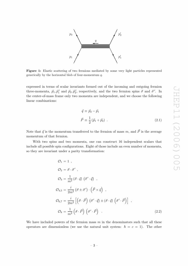
In order to derive the long-range force between two fermions of masses m and m′, mediated

by some very light particles, one needs to compute first the nonrelativistic limit of the

scattering amplitude represented by the diagram shown in figure 1. This amplitude can be

– 2 –

JHEP11(2006)005

AA

AA

AA

AA

AAK

¢¢

¢¢

¢¢¢¢̧

¢¢¢¢¢¢

¢¢¢¢̧

AAAAAA

AAK

¾q

p2

p1

p′2

p′1

Figure 1: Elastic scattering of two fermions mediated by some very light particles represented

generically by the horizontal blob of four-momentum q.

expressed in terms of scalar invariants formed out of the incoming and outgoing fermion

three-momenta, ~p1, ~p′1 and ~p2, ~p

′2 , respectively, and the two fermion spins ~σ and ~σ ′. In

the center-of-mass frame only two momenta are independent, and we choose the following

linear combinations:

~q ≡ ~p2 − ~p1

~P ≡ 1

2(~p1 + ~p2) . (2.1)

Note that ~q is the momentum transferred to the fermion of mass m, and ~P is the average

momentum of that fermion.

With two spins and two momenta, one can construct 16 independent scalars that

include all possible spin configurations. Eight of those include an even number of momenta,

so they are invariant under a parity transformation:

O1 = 1 ,

O2 = ~σ · ~σ ′ ,

O3 =1

m2(~σ · ~q)

(

~σ ′ · ~q)

,

O4,5 =i

2m2

(

~σ ± ~σ ′)

·(

~P × ~q)

,

O6,7 =i

2m2

[(

~σ · ~P)

(

~σ ′ · ~q)

± (~σ · ~q)(

~σ ′ · ~P)]

,

O8 =1

m2

(

~σ · ~P) (

~σ ′ · ~P)

. (2.2)

We have included powers of the fermion mass m in the denominators such that all these

operators are dimensionless (we use the natural unit system: ~ = c = 1). The other

– 3 –

JHEP11(2006)005

eightscalars change sign under a parity transformation:

O9,10 =i

2m

(

~σ ± ~σ ′)

· ~q ,

O11 =i

m

(

~σ × ~σ ′)

· ~q ,

O12,13 =1

2m

(

~σ ± ~σ ′)

· ~P ,

O14 =1

m

(

~σ × ~σ ′)

· ~P ,

O15 =1

2m3

{

[

~σ ·(

~P × ~q)]

(

~σ ′ · ~q)

+ (~σ · ~q)[

~σ ′ ·(

~P × ~q)]

}

O16 =i

2m3

{

[

~σ ·(

~P × ~q)] (

~σ ′ · ~P)

+(

~σ · ~P) [

~σ ′ ·(

~P × ~q)]

}

. (2.3)

Any other scalar operator involving at least one of the two spins can be expressed as a

linear combination of the operators Oi(~q, ~P ), i = 1, . . . , 16, with coefficients that may

depend on the momenta only through the ~q 2 or ~P 2 scalars. Note that energy-momentum

conservation implies ~q· ~P = 0. Examples of other operators which can be expressed as linear

combinations of Oi, i = 1, . . . , 16, can be found in appendix A. Although several of the

operators given in eq. (2.2) have been analyzed in the context of nuclear interactions [19 –

21], we believe that the complete set of 16 rotationally invariant operators has not been

previously presented in the literature.

The amplitude for elastic scattering of the two fermions depends on the properties of

the light particles that mediate it. The long-range nature of the force is due to the propa-

gator of the exchanged particles, which is a function of the square of the four-momentum

transferred, q2. Energy and momentum conservation require the energy transfer to be

exactly zero, q0 = 0, so that q2 = −~q 2. We use P(~q 2,m0) to denote the imaginary part

of the propagator with the Lorentz structure factored out. The mass dimension of P(~q 2)

is −2. In the most common case, where the potential is induced by the exchange of one

boson within a Lorentz invariant quantum field theory,

P(~q 2) = − 1

~q 2 + m20

, (2.4)

where m0 is the mass of the boson. Other forms for the propagator are possible. For

example, in the case where two massless fermions are exchanged, the effective propagator

takes the form [22]

P(~q 2) = − 1

12π2M2ln

(

~q 2

M2

)

, (2.5)

where M is the mass scale that suppresses the four-fermion contact interaction. If Lorentz

symmetry is violated, then a boson may have a kinetic term with four or more spatial

derivatives, giving a propagator

P(~q 2) = −M2k−2

(~q 2)k, (2.6)

– 4 –

JHEP11(2006)005

where k ≥ 2 is an integer, and M is some mass scale. The case k = 2 has been studied

in [18]. For the moment we allow a generic form for P(~q 2), assuming only that it leads to

long-range forces.

Certain generic features of the amplitude can be derived on general grounds. The

nonrelativistic amplitude between two fermions may be written in the momentum space

as

A(

~q, ~P)

= P(~q 2)

16∑

i=1

Oi

(

~q, ~P)

fi

(

~q 2/m2, ~P 2/m2)

, (2.7)

where fi are dimensionless scalar functions. In the nonrelativistic limit, fi are polynomials

with coefficients that depend on the couplings of the exchanged particles. This is a general

result based only on the assumption of rotational invariance (this assumption is not valid

in certain Lorentz-violating field theories [18, 23]).

The physical interpretation of the 16 operators is more transparent in the position

space, as discussed in the next section.

3. Long-range potentials between fermions

The Fourier transform of the momentum-space amplitude with respect to the momentum

transfer ~q gives the position-space potential:

V (~r,~v) = −∫

d3q

(2π)3ei~q·~r A(~q,m~v ) , (3.1)

where ~r is the position vector of the fermion of mass m and initial momentum ~p1 with

respect to the fermion of mass m′ and initial momentum ~p ′1. Note that in general the

potential depends not only on the position ~r, but also on the average velocity of the

fermion of mass m in the center-of-mass frame:

~v =~P

m. (3.2)

The inverse mass of the boson sets the range of the interaction, so that an experimental

setup characterized by a distance scale rexp is sensitive to 1/m0 ∼> rexp. We assume that

rexp is macroscopic, rexp ∼> O(1 mm), The most important contributions to the potential

come from the momentum-independent terms of the fi

(

~q 2/m2, ~v 2)

polynomials in eq. (2.7).

Additional powers of ~q 2/m2 lead to terms of order ε2 in the potential, where ε is of the

order of m0/m or 1/(rexpm) (see appendix B). Given that m is the mass of the electron

or nucleon, we find ε < 10−10, so that it is a good approximation to include only the

~q 2 = 0 pieces of the polynomials, fi

(

0, ~v 2)

. Note that additional powers of ~q 2/m2 also

lead to Fourier transforms of the type δ(~r), or more singular ones, which describe contact

interactions rather than long-range potentials.

It is useful to observe that compared to O1 and O2, the operators Oi with i = 9, 10, 11

have effects of order ε, the operators Oi with i = 12, 13, 14 have effects of order v = |~v|,while the remaining ones have effects suppressed by more powers of ε or v. If the ~q 2-

independent term of fi vanishes, then the ~q 2/m2 term dominates, and for i = 1, 2, 9, . . . , 14

– 5 –

JHEP11(2006)005

it might lead to experimentally observable effects. By contrast, the operators Oi with

i = 3, . . . , 8, 15, 16 are already quite suppressed, so that the ~q 2-dependent terms of fi

can be safely neglected in their case. In what follows we will ignore the ~q 2-dependent

terms of all fi, and we only mention that if a physical situation would require the in-

clusion of some of them, then they could be treated similarly to the ~q 2-independent

terms.

The long-range potential between two fermions induced by a Lorentz-invariant, one-

boson exchange can be written as

V (~r,~v) =

16∑

i=1

Vi (~r,~v) fi

(

0, ~v 2)

, (3.3)

where we defined a complete set of spin-dependent potentials,

Vi(~r,~v) = −∫

d3q

(2π)3ei~q·~r P(~q 2)Oi(~q,m~v) , (3.4)

with i = 1, . . . , 16. As stated before, fi(0, ~v2) are polynomials in ~v 2, with coefficients given

by dimensionless parameters that depend on the boson couplings to the fermions.

It is convenient to write the spin-dependent potentials in terms of a dimensionless

function of r:

y(r) ≡ −r

∫

d3q

(2π)3ei~q·~r P(~q 2)

= − 1

2π2

∫ ∞

0

d|~q| P(~q 2) |~q| sin (|~q|r) . (3.5)

Using the operators Oi with i = 1, . . . , 8, defined in eq. (2.2), we obtain the following

long-range, parity-invariant potentials:

V1 =1

ry(r) ,

V2 =1

r~σ · ~σ ′ y(r) ,

V3 =1

m2 r3

[

~σ · ~σ ′

(

1 − rd

dr

)

− 3(

~σ · ~̂r) (

~σ ′ · ~̂r)

(

1 − rd

dr+

1

3r2 d2

dr2

)]

y(r) ,

V4,5 = − 1

2m r2

(

~σ ± ~σ ′)

·(

~v × ~̂r)

(

1 − rd

dr

)

y(r) ,

V6,7 = − 1

2m r2

[

(~σ · ~v)(

~σ ′ · ~̂r)

±(

~σ · ~̂r)

(

~σ ′ · ~v)

] (

1 − rd

dr

)

y(r) ,

V8 =1

r(~σ · ~v)

(

~σ ′ · ~v)

y(r) , (3.6)

where r is the length of the ~r vector, and we have defined the unit vector

~̂r ≡ ~r

r. (3.7)

– 6 –

JHEP11(2006)005

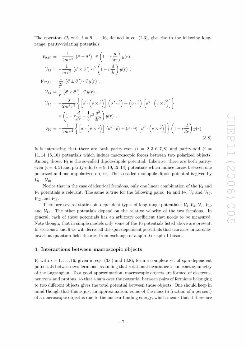
The operators Oi with i = 9, . . . , 16, defined in eq. (2.3), give rise to the following long-

range, parity-violating potentials:

V9,10 = − 1

2m r2

(

~σ ± ~σ ′)

· ~̂r(

1 − rd

dr

)

y(r) ,

V11 = − 1

m r2

(

~σ × ~σ ′)

· ~̂r(

1 − rd

dr

)

y(r) ,

V12,13 =1

2r

(

~σ ± ~σ ′)

· ~v y(r) ,

V14 =1

r

(

~σ × ~σ ′)

· ~v y(r) ,

V15 = − 3

2m2 r3

{

[

~σ ·(

~v × ~̂r)] (

~σ ′ · ~̂r)

+(

~σ · ~̂r) [

~σ ′ ·(

~v × ~̂r)]

}

×(

1 − rd

dr+

1

3r2 d2

dr2

)

y(r) ,

V16 = − 1

2m r2

{

[

~σ ·(

~v × ~̂r)]

(

~σ ′ · ~v)

+ (~σ · ~v)[

~σ ′ ·(

~v × ~̂r)]

} (

1 − rd

dr

)

y(r) .

(3.8)

It is interesting that there are both parity-even (i = 2, 3, 6, 7, 8) and parity-odd (i =

11, 14, 15, 16) potentials which induce macroscopic forces between two polarized objects.

Among those, V3 is the so-called dipole-dipole potential. Likewise, there are both parity-

even (i = 4, 5) and parity-odd (i = 9, 10, 12, 13) potentials which induce forces between one

polarized and one unpolarized object. The so-called monopole-dipole potential is given by

V9 + V10.

Notice that in the case of identical fermions, only one linear combination of the V4 and

V5 potentials is relevant. The same is true for the following pairs: V6 and V7, V9 and V10,

V12 and V13.

There are several static spin-dependent types of long-range potentials: V2,V3, V9, V10

and V11. The other potentials depend on the relative velocity of the two fermions. In

general, each of these potentials has an arbitrary coefficient that needs to be measured.

Note though, that in simple models only some of the 16 potentials listed above are present.

In sections 5 and 6 we will derive all the spin-dependent potentials that can arise in Lorentz-

invariant quantum field theories from exchange of a spin-0 or spin-1 boson.

4. Interactions between macroscopic objects

Vi with i = 1, . . . , 16, given in eqs. (3.6) and (3.8), form a complete set of spin-dependent

potentials between two fermions, assuming that rotational invariance is an exact symmetry

of the Lagrangian. To a good approximation, macroscopic objects are formed of electrons,

neutrons and protons, so that a sum over the potential between pairs of fermions belonging

to two different objects gives the total potential between those objects. One should keep in

mind though that this is just an approximation: some of the mass (a fraction of a percent)

of a macroscopic object is due to the nuclear binding energy, which means that if there are

– 7 –

JHEP11(2006)005

long-range forces between electrons and gluons, for example, then their effects would not

be fully taken into account by summing over fermion pairs.

In section 2 we have argued that the propagator of the very light particles that mediate

macroscopic forces may have various forms. In this section we first discuss the case of

standard propagator, given in eq. (2.4), and later in subsection 4.2 we consider other forms

for the propagator, as in eqs. (2.5) and (2.6).

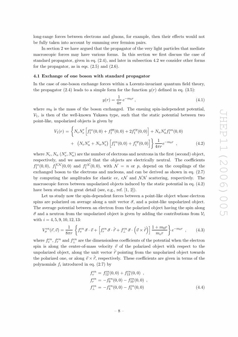
4.1 Exchange of one boson with standard propagator

In the case of one-boson exchange forces within a Lorentz-invariant quantum field theory,

the propagator (2.4) leads to a simple form for the function y(r) defined in eq. (3.5):

y(r) =1

4πe−m0r , (4.1)

where m0 is the mass of the boson exchanged. The ensuing spin-independent potential,

V1, is then of the well-known Yukawa type, such that the static potential between two

point-like, unpolarized objects is given by

V1(r) =

{

NeN′e

[

f ee1 (0, 0) + fpp

1 (0, 0) + 2f ep1 (0, 0)

]

+ NnN ′nfnn

1 (0, 0)

+(

NeN′n + NnN ′

e

)

[

f en1 (0, 0) + f ep

1 (0, 0)]

}

1

4πre−m0r , (4.2)

where Ne, Nn (N ′e, N

′n) are the number of electrons and neutrons in the first (second) object,

respectively, and we assumed that the objects are electrically neutral. The coefficients

f ee1 (0, 0), fNN

1 (0, 0) and f eN1 (0, 0), with N = n or p, depend on the couplings of the

exchanged boson to the electrons and nucleons, and can be derived as shown in eq. (2.7)

by computing the amplitudes for elastic ee, eN and NN scattering, respectively. The

macroscopic forces between unpolarized objects induced by the static potential in eq. (4.2)

have been studied in great detail (see, e.g., ref. [1, 2]).

Let us study now the spin-dependent forces between a point-like object whose electron

spins are polarized on average along a unit vector ~σ, and a point-like unpolarized object.

The average potential between an electron from the polarized object having the spin along

~σ and a neutron from the unpolarized object is given by adding the contributions from Vi

with i = 4, 5, 9, 10, 12, 13:

V enσ (~r,~v) =

1

8πr

{

f env ~σ · ~v +

[

f enr ~σ · ~̂r + f en

⊥ ~σ ·(

~v × ~̂r)] 1 + m0r

mer

}

e−m0r , (4.3)

where f env , f en

r and f en⊥ are the dimensionless coefficients of the potential when the electron

spin is along the center-of-mass velocity ~v of the polarized object with respect to the

unpolarized object, along the unit vector ~̂r pointing from the unpolarized object towards

the polarized one, or along ~v × ~̂r, respectively. These coefficients are given in terms of the

polynomials fi introduced in eq. (2.7) by

f env = f en

12 (0, 0) + f en13 (0, 0) ,

f enr = −f en

9 (0, 0) − f en10 (0, 0) ,

f en⊥ = −f en

4 (0, 0) − f en5 (0, 0) (4.4)

– 8 –

JHEP11(2006)005

where the upper indices e and n indicate that the fermions of mass m and m′ discussed in

general in sections 2 and 3 are now specified to be an electron and a neutron, respectively.

We have included only the ~q 2- and ~P 2- independent terms in fi because the ~q 2-dependent

terms give tiny corrections of order (m0/me)2 while ~P 2-dependent terms give relativistic

corrections which are also negligible in experiments searching for new macroscopic forces.

The average potential between the electron spin and the protons or electrons in the

unpolarized object, V epσ and V ee

σ , respectively, may be written analogously to eq. (4.3).

Then the total potential between the object containing the polarized electrons and the

unpolarized object is

Vσe(~r,~v) = Neσe

[

N ′p (V ee

σ + V epσ ) + N ′

nV enσ

]

, (4.5)

where Ne is the total number of electrons in the polarized object, σe is the polarization (the

average projection of the electron spins along ~σ in the polarized object), N ′p and N ′

n are the

numbers of protons and neutrons in the unpolarized object. In writing the above equation

we have assumed that the unpolarized object is electrically-neutral. If the polarized object

has the neutrons or protons polarized instead of the electrons, then the potentials V nσ (~r,~v)

or V pσ (~r,~v) are given by eq. (4.5) with the index e replaced appropriately by n or p in

eqs. (4.3)-(4.5). If the boson exchange induces in addition a spin-independent potential,

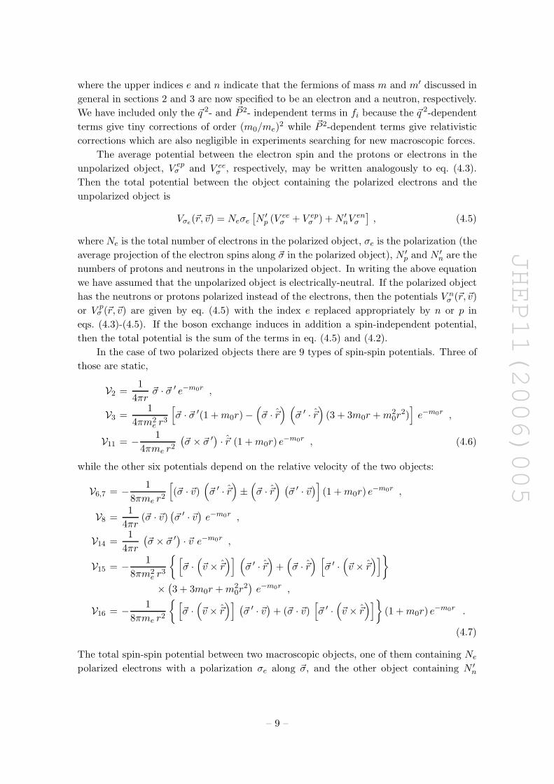
then the total potential is the sum of the terms in eq. (4.5) and (4.2).

In the case of two polarized objects there are 9 types of spin-spin potentials. Three of

those are static,

V2 =1

4πr~σ · ~σ ′ e−m0r ,

V3 =1

4πm2e r3

[

~σ · ~σ ′(1 + m0r) −(

~σ · ~̂r) (

~σ ′ · ~̂r)

(3 + 3m0r + m20r

2)]

e−m0r ,

V11 = − 1

4πme r2

(

~σ × ~σ ′)

· ~̂r (1 + m0r) e−m0r , (4.6)

while the other six potentials depend on the relative velocity of the two objects:

V6,7 = − 1

8πme r2

[

(~σ · ~v)(

~σ ′ · ~̂r)

±(

~σ · ~̂r)

(

~σ ′ · ~v)

]

(1 + m0r) e−m0r ,

V8 =1

4πr(~σ · ~v)

(

~σ ′ · ~v)

e−m0r ,

V14 =1

4πr

(

~σ × ~σ ′)

· ~v e−m0r ,

V15 = − 1

8πm2e r3

{

[

~σ ·(

~v × ~̂r)] (

~σ ′ · ~̂r)

+(

~σ · ~̂r) [

~σ ′ ·(

~v × ~̂r)]

}

×(

3 + 3m0r + m20r

2)

e−m0r ,

V16 = − 1

8πme r2

{

[

~σ ·(

~v × ~̂r)]

(

~σ ′ · ~v)

+ (~σ · ~v)[

~σ ′ ·(

~v × ~̂r)]

}

(1 + m0r) e−m0r .

(4.7)

The total spin-spin potential between two macroscopic objects, one of them containing Ne

polarized electrons with a polarization σe along ~σ, and the other object containing N ′n

– 9 –

JHEP11(2006)005

polarized neutrons with a polarization σn along ~σ′, is given by

Vσeσ′

n

(~r,~v) = NeσeN′nσ′

n

∑

i

f eni (0, 0)Vi(~r,~v) , (4.8)

where the sum is over the potentials shown in eqs. (4.6) and (4.7). An analogous potential

exists for two objects containing polarized electrons, except that all n indices are replaced

by e, and the f eni (0, 0) coefficients may be obtained by computing the ee → ee amplitude.

Similar statements apply to the ep, pp, nn or np spin-spin potentials. Notice that several

of the potentials in eqs. (4.6) and (4.7) include an inverse power of the electron mass, me,

introduced to keep the fi functions dimensionless. In the case of the potentials between

nucleons, me is replaced by mn (or else the fi functions need to be rescaled appropriately).

We briefly discuss the experimental limits on the coefficients of the various potentials.

Tests of the equivalence principle and of the inverse square law set limits on the Yukawa

potential between unpolarized objects. Given that the tests involve macroscopic objects

which are electrically neutral, the boson couplings to the electron and proton are not con-

strained separately. Only their sum is constrained at roughly the same level as the neutron

vector coupling. Thus, the limits may be expressed in terms of the three combinations of

f1 coefficients that appear in eq. (4.2):

|fnn1 (0, 0)| , |f en

1 (0, 0) + f ep1 (0, 0)| , |f ee

1 (0, 0) + fpp1 (0, 0) + 2f ep

1 (0, 0)| < 10−40 − 10−48 ,

(4.9)

where the weaker limit applies to 1/m0 of order 1 cm, while the stronger one applies to

1/m0 > 108 m, the Earth-Moon distance (see figure 4 of [1]).

The most stringent limit on the dipole-dipole potential V3 between electrons is set in

ref. [8] (see also [6, 7], where the potential is explicitly written:1) 1.2 ± 2.0 × 10−14 times

the magnetic interaction of two electrons, for 1/m0 ∼> 10 cm. At the 1σ confidence level

we then find

−0.8 × 10−14 <f ee3 (0, 0)

4π2α< 3.2 × 10−14 . (4.10)

Similarly, the limit on the dipole-dipole potential between an electron and a neutron [5]

gives|f en

3 (0, 0)|4π2α|µn/µN | < 2.3 × 10−11 , (4.11)

for 1/m0 ∼> 1 m. Here |µn/µN | ≈ 1.913 is the ratio of the neutron magnetic moment to the

nuclear magneton. The limits on the dipole-dipole potential between nucleons, or between

an electron and a proton are weaker [5].

The static spin-spin potential V2 has not been experimentally searched for. However,

the limits on the dipole-dipole potential V3 provide an indirect constraint on V2. It is not

clear how accurate would be the use of the best limits on V3, given in ref. [8] and [5], to

constrain V2, because V3 includes a (σ · ~r)(σ′ · ~r) piece which is not present in V2. By

contrast, the limit set in ref. [4] explicitly applies to the σ · σ′ piece of the dipole-dipole

1The potential shown in eq. (1) of ref. [7] falls off as 1/r instead of 1/r3. We believe that this is just a

typo.

– 10 –

JHEP11(2006)005

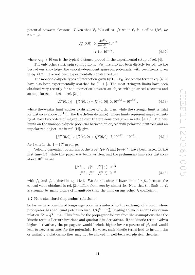
potential between electrons. Given that V2 falls off as 1/r while V3 falls off as 1/r3, we

estimate

|f ee2 (0, 0)| ∼<

4π2α

m2er

2exp

10−11

≈ 4 × 10−35 , (4.12)

where rexp ≈ 10 cm is the typical distance probed in the experimental setup of ref. [4].

The only other static spin-spin potential, V11, has also not been directly tested. To the

best of our knowledge, the velocity-dependent spin-spin potentials, with coefficients given

in eq. (4.7), have not been experimentally constrained yet.

The monopole-dipole types of interaction given by V9+V10 [see second term in eq. (4.3)]

have also been experimentally searched for [9 – 11]. The most stringent limits have been

obtained very recently for the interaction between an object with polarized electrons and

an unpolarized object in ref. [24]:

|f enr (0, 0)| , |f ee

r (0, 0) + f epr (0, 0)| ∼< 10−30 − 10−36 , (4.13)

where the weaker limit applies to distances of order 1 m, while the stronger limit is valid

for distances above 1011 m (the Earth-Sun distance). These limits represent improvements

by at least two orders of magnitude over the previous ones given in refs. [9, 10]. The best

limits on the monopole-dipole potential between an object with polarized neutrons and an

unpolarized object, set in ref. [12], give

|fnnr (0, 0)| , |fne

r (0, 0) + fnpr (0, 0)| ∼< 10−27 − 10−33 , (4.14)

for 1/m0 in the 1 − 106 m range.

Velocity dependent potentials of the type V4+V5 and V12+V13 have been tested for the

first time [24] while this paper was being written, and the preliminary limits for distances

above 1011 m are

|f en⊥ | ,

∣

∣f ee⊥ + f ep

⊥

∣

∣ ∼< 10−32 ,

f env , f ee

v + f epv ∼< 10−55 , (4.15)

with f⊥ and fv defined in eq. (4.4). We do not show a lower limit for fv, because the

central value obtained in ref. [24] differs from zero by almost 2σ. Note that the limit on fv

is stronger by many orders of magnitude than the limit on any other fi coefficient.

4.2 Non-standard dispersion relations

So far we have considered long-range potentials induced by the exchange of a boson whose

propagator has the usual pole structure, 1/(q2 − m20), leading to the standard dispersion

relation E2 = ~q 2+m20 . This form for the propagator follows from the assumptions that the

kinetic term is Lorentz invariant and quadratic in derivatives. If the kinetic term involves

higher derivatives, the propagator would include higher inverse powers of q2, and would

lead to new structures for the potentials. However, such kinetic terms lead to instabilities

or unitarity violation, so they may not be allowed in well-behaved physical theories.

– 11 –

JHEP11(2006)005

AA

AA

AA

AA

AAK

¢¢

¢¢

¢¢¢¢̧

¢¢¢¢¢¢

¢¢¢¢̧

AAAAAA

AAK

¾~q

γ′

~P + 12~q

e−

~P − 12~q

e−

−~P − 12~q

e− (N)

−~P + 12~q

e− (N)

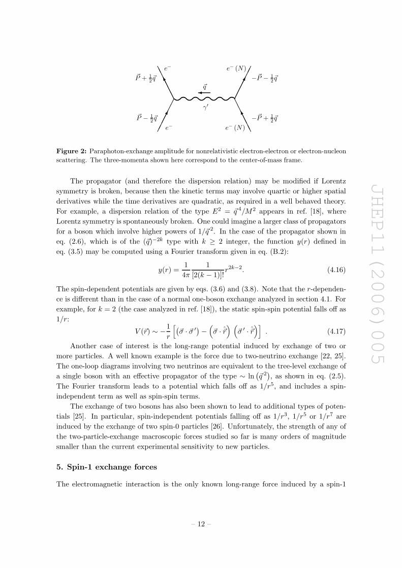
Figure 2: Paraphoton-exchange amplitude for nonrelativistic electron-electron or electron-nucleon

scattering. The three-momenta shown here correspond to the center-of-mass frame.

The propagator (and therefore the dispersion relation) may be modified if Lorentz

symmetry is broken, because then the kinetic terms may involve quartic or higher spatial

derivatives while the time derivatives are quadratic, as required in a well behaved theory.

For example, a dispersion relation of the type E2 = ~q 4/M2 appears in ref. [18], where

Lorentz symmetry is spontaneously broken. One could imagine a larger class of propagators

for a boson which involve higher powers of 1/~q 2. In the case of the propagator shown in

eq. (2.6), which is of the (~q)−2k type with k ≥ 2 integer, the function y(r) defined in

eq. (3.5) may be computed using a Fourier transform given in eq. (B.2):

y(r) =1

4π

1

[2(k − 1)]!r2k−2. (4.16)

The spin-dependent potentials are given by eqs. (3.6) and (3.8). Note that the r-dependen-

ce is different than in the case of a normal one-boson exchange analyzed in section 4.1. For

example, for k = 2 (the case analyzed in ref. [18]), the static spin-spin potential falls off as

1/r:

V (~r) ∼ −1

r

[

(

~σ · ~σ ′)

−(

~σ · ~̂r) (

~σ ′ · ~̂r)]

. (4.17)

Another case of interest is the long-range potential induced by exchange of two or

more particles. A well known example is the force due to two-neutrino exchange [22, 25].

The one-loop diagrams involving two neutrinos are equivalent to the tree-level exchange of

a single boson with an effective propagator of the type ∼ ln(

~q 2)

, as shown in eq. (2.5).

The Fourier transform leads to a potential which falls off as 1/r5, and includes a spin-

independent term as well as spin-spin terms.

The exchange of two bosons has also been shown to lead to additional types of poten-

tials [25]. In particular, spin-independent potentials falling off as 1/r3, 1/r5 or 1/r7 are

induced by the exchange of two spin-0 particles [26]. Unfortunately, the strength of any of

the two-particle-exchange macroscopic forces studied so far is many orders of magnitude

smaller than the current experimental sensitivity to new particles.

5. Spin-1 exchange forces

The electromagnetic interaction is the only known long-range force induced by a spin-1

– 12 –

JHEP11(2006)005

particle. Nevertheless, low-mass spin-1 particles other than the photon may exist, and

they would lead to additional long-range forces that could be searched for in experiments.

5.1 New massless gauge boson

A spin-1 particle is naturally kept massless by an unbroken gauge symmetry. In particular,

a new U(1) gauge symmetry would require the existence of a massless spin-1 particle,

labeled γ′ and called paraphoton [27]. If any of the Standard Model fields would be

charged under the new U(1) symmetry, then the gauge anomaly cancellation requires the

U(1) charge to be proportional to the B − L number, so that the γ′ coupling to any

electrically-neutral macroscopic object is proportional to the number of neutrons [17]. As

a result, such couplings can be probed through tests of the equivalence principle and of

the inverse square law (see [28] for a related discussion). The ensuing upper limit on the

gauge coupling of the paraphoton is orders of magnitude below the gravitational coupling

of the proton, mp/MPlanck ≈ 10−19. This appears to be unnaturally small and also poses

theoretical challenges [29].

It is possible, however, that all Standard Model fields have zero charge under the

new U(1) symmetry, and yet γ′ may interact with the quarks and leptons via dimension-6

operators involving two fermion fields, a paraphoton, and a Higgs doublet [17]. Those

operators are gauge invariant and do not depend on the fermion charges. Replacing the

Higgs doublet by its vacuum expectation value (VEV), vh ' 174 GeV, yields dimension-5

operators in the Lagrangian, representing magnetic- and electric-like dipole moments:

Lγ′ =vh

M2Pµν

e σµν(ReCe + iImCeγ5) e +∑

N=n,p

Nσµν(ReCN + iImCN γ5)N

. (5.1)

Here Pµν is the field strength of the paraphoton, e is the electron field, N is the nucleon field,

while Ce and CN are dimensionless complex parameters (their values are expected to be

much less than unity). The γ′ coupling to nucleons is an effective low-energy Lagrangian

that arises from a similar coupling of γ′ to u or d quarks. These couplings may have

different strengths, and therefore the values of CN when N is a proton or a neutron may be

different. The mass M sets the scale where the dimension-6 operators are generated within

an underlying theory which is well-behaved in the ultraviolet (examples of renormalizable

models of this type are given in [17]).

One γ′ exchange between electrons or nucleons leads to a long-range force between

chunks of ordinary matter. In figure 2 we show the three-momentum flow for the scattering

of fermions mediated by γ′. The amplitude for this process is given by

A(

~q, ~P)

= − 1

~q 2

4v2h

M4SνS′

ν , (5.2)

where ν = 0, 1, 2, 3 is a Lorentz index, and we have defined

Sν = ue(P + q/2) qµσµν(ReCe + iImCeγ5) ue(P − q/2) . (5.3)

The spinor ue(p) describes the electron field of four-momentum p. In the case of e−e− scat-

tering, S′ν is identical to Sν except for the spinor ue(p′) which depends on the momentum

– 13 –

JHEP11(2006)005

of the second electron. In the case of e−N scattering, S′ν has the same structure as Sν

but the nucleon spinor uN (p′) and complex parameter CN replace the electron ones.

In what follows we compute the nonrelativistic amplitude for e−N scattering, because

the result can be immediately adapted to e−e− or NN scattering. In the nonrelativistic

limit, the time-like component of Sν is given by

S0 = −ImCe ~q · ~σ +1

meReCe

[

(

~P × ~q)

· ~σ − i

2~q 2

]

. (5.4)

Relativistic corrections to S0, of order ~P 2/m2e and ~q 2/m2

e, do not introduce new spin-

dependent terms. For the nucleon of initial three-momentum −~P + ~q/2,

S′0 = ImCN ~q · ~σ ′ +1

mNReCN

[

(

~P × ~q)

· ~σ ′ − i

2~q 2

]

. (5.5)

In order to compute the space-like components of Sν and S′ν , it is useful to recall that

energy-momentum conservation implies ~P · ~q = 0 and q0 = 0. We find

~S = ReCe

[

~q × ~σ − i~q 2

4m2e

~P +1

m2e

(

~P · ~σ)

~P × ~q

]

− 1

meImCe (~q · ~σ) ~P ,

~S′= −ReCN

[

~q × ~σ ′ − i~q 2

4m2N

~P +1

m2N

(

~P · ~σ ′)

~P × ~q

]

− 1

mNImCN

(

~q · ~σ ′)

~P , (5.6)

with relativistic corrections affecting only the above spin-dependent terms.

A lengthy but straightforward computation of the right-hand side of eq. (5.2) then

gives the nonrelativistic amplitude. For the purpose of deriving the long-range potential,

we may ignore the terms in SνS′ν proportional to ~q 2, because upon Fourier transforming to

position space they give only contact interactions or contributions additionally suppressed

by m0, as discussed in section 3.1. The result takes the form of eq. (2.7), with the functions

fi

(

0, ~v 2)

being nonzero only for i = 3, 15. In the nonrelativistic limit, keeping only the

leading order in ~v 2, we obtain the following values for these functions:

f eN3 (0, 0) = −4v2

hm2e

M4Re (C∗

e CN ) ,

f eN15 (0, 0) =

4v2hm2

e

M4

(

1 +me

mN

)

[

Re (Ce) Im (CN ) − Im (Ce)Re (CN )]

. (5.7)

Therefore, the long-range potential between an electron and a nucleon induced by γ′ ex-

change is given by

VeN (~r,~v) =∑

i=3,15

Vi (~r,~v)

∣

∣

∣

∣

m=me

f eNi (0, 0) (5.8)

where the parity-even potential V3 is given in eq. (3.6) while the parity-odd potential V15

is given in eq. (3.8). Notice that the long-range potential induced by paraphoton exchange

may be observed only if both objects are polarized.

The long-range potential between electrons due to γ′ may be obtained from eqs. (5.8)

and (5.7) by replacing the subscript N by e (note that f ee15 = 0, so that the long-range

– 14 –

JHEP11(2006)005

potential is static in this case):

Vee (~r,~v) = −4v2hm2

e

M4|Ce|2 V3

∣

∣

∣

∣

m=me

. (5.9)

The proton-proton and neutron-neutron long-range potentials have analogous forms with

the appropriate replacements of me and Ce by the proton and neutron parameters. The

proton-neutron potential may include in addition the V15 spin-dependent potential, simi-

larly to eq. (5.8). Note that the only static potential induced by γ′ exchange is V3, which

gives the usual long-range force between two magnetic dipole moments but with an overall

strength that depends on the γ′ couplings.

Given that the dimension-six operators that give rise to the effective γ′ couplings

in eq. (5.1) involve a chirality flip of the fermions, it is expected that its dimensionless

coefficients are of the order of or smaller than the corresponding Yukawa coupling to the

Higgs doublet. It is therefore useful to factor out the Yukawa coupling from the Ce and

CN parameters:

ce ≡ vh

me|Ce| ,

cN ≡ vh

md|CN | , (5.10)

where md is the down-quark mass. The parameters ce and cN may be as large as O(1), but

could be orders of magnitude smaller than one if the dimension-6 operators are generated

at loop level in some renormalizable model with weakly coupled fields. The experimental

limits on the paraphoton coupling to the electrons and nucleons can be expressed in terms

of M/√

ce and M/√

cN , respectively.

The static potential between electrons induced by γ′ exchange takes the form

V (~r) = − c2em

2e

πM4r3

[

~σ1 · ~σ2 − 3(

~σ1 · ~̂r) (

~σ2 · ~̂r)]

, (5.11)

so that it is an attractive V3 potential. Using the 1σ limit shown in eq. (4.10), we find

c2em

4e

π2αM4< 0.8 × 10−14 , (5.12)

where α is the fine structure constant. This translates into a limit

M√ce

> 3.3 GeV . (5.13)

Similarly, the limit on the dipole-dipole potential between an electron and a neutron [5],

shown in eq. (4.11), gives

cecN m2emdmp

π2αM4|µn/µN | cos (θe − θN ) < 2.3 × 10−11 , (5.14)

where θe,N are the complex phases of Ce,N and mp is the proton mass. We find the following

constraint on the paraphoton couplings:

M√cecN

cos−1/4(θe − θN ) > 4.2 GeV . (5.15)

– 15 –

JHEP11(2006)005

where we used md ∼ 4 MeV.

The bounds from star cooling on M/√

ce and M/√

cN are three orders of magnitude

stronger than eqs. (5.13) and (5.15), while the limits from primordial nucleosynthesis are

also substantially stronger (M/√

ce ∼> 100 GeV and M/√

cN ∼> 400 GeV) [17]. However,

there are potential loopholes in these astrophysical and cosmological limits, whereas the

limit from searches for new macroscopic forces is robust. A well known loophole in the limit

from primordial nucleosynthesis is the possibility of a chemical potential during the early

Universe. The limits from star cooling, considered unavoidable in the case of axions [16],

could be avoided in the case of the paraphoton if the properties of this massless gauge boson

depend on temperature. We contemplate a theory that besides the Standard Model and the

new U(1) gauge group includes two or more scalar fields such that there is a mechanism of

symmetry non-restoration at high temperatures [30]. Specifically, if a scalar charged under

the new U(1) acquires a VEV when in thermal equilibrium in a star, and if this VEV

is larger than the star temperature, then the γ′ emission from the star is exponentially

suppressed. As a result, star cooling via γ′ emission could be negligible.

5.2 General spin-1 exchange

So far we have discussed the case of a massless spin-1 field which couples to electrons or

nucleons via higher-dimensional operators. Let us turn now to a more general Lorentz-

invariant extension of the Standard Model that includes a new spin-1 field, Z ′, that is

electrically neutral. We assume that its mass m0 is nonzero but smaller than 10−3 eV, so

that Z ′ exchange mediates forces with a range longer than a micrometer. We will consider

in some cases a mass as small as 10−18 eV, which is the inverse Earth-Sun distance.

Without loss of generality, we assume that such a Z ′ field is the gauge boson associated

with a new U(1)z gauge symmetry that is spontaneously broken by the VEV of a spin-0

field ϕ, which is a singlet under the Standard Model gauge group. The Z ′ mass is then

related to the gauge coupling gz and the ϕ charge zϕ:

m0 = zϕgz〈ϕ〉 . (5.16)

If the Higgs doublet carries a U(1)z charge zH , then there is mixing between the Z and Z ′

bosons, and the above equation is modified (see eq. (2.6) of ref. [31]). However, here we

require m0 ¿ MZ which implies zHgz ¿ 1 such that the corrections to eq. (5.16) are very

small.

The Z ′ boson couples to the leptons and quarks of the first generation as follows:

LgZ′ = gzZ

′µ

(

zl lLγµlL + ze eRγµeR + zq qLγµqL + zu uRγµuR + zd dRγµdR

)

, (5.17)

where qL = (uL, dL) and lL = (νL, eL) are SU(2)W doublets, while zl, ze, zq, zu, and zd are

the U(1)z charges of the leptons and quarks. The ensuing couplings at low energy of the

Z ′ boson to electrons and nucleons are given by

Z ′µ

eγµ (geV + ge

Aγ5) e +∑

N=n,p

Nγµ(

gNV + γ5gNA

)

N

, (5.18)

– 16 –

JHEP11(2006)005

where the vector and axial couplings of the electron, proton and neutron are

geV,A =

gz

2(ze ± zl) ,

gpV,A =

gz

2(2zu + zd ± 3zq) ,

gnV,A =

gz

2(zu + 2zd ± 3zq) . (5.19)

In addition to these dimension-4 interactions, there are higher-dimensional interactions

as in eq. (5.1), with Pµν = ∂µZ ′ν − ∂νZ ′

µ, describing magnetic- and electric-like dipole

couplings.

The U(1)z charges may be treated as arbitrary real parameters. However, there are

various requirements that any self-consistent theory that includes the U(1)z gauge group

has to satisfy. The SU(3)C ×SU(2)W ×U(1)Y ×U(1)z gauge theory must be anomaly free,

so that the U(1)z charges must satisfy several cubic and linear equations. Furthermore,

the quark and lepton charges are expected to be commensurate numbers (i.e., their ratios

are rational numbers), which makes it much harder to satisfy the cubic equations. It turns

out [32], however, that all anomaly cancellation conditions may be satisfied while keeping

zl, ze, zq, zu, and zd arbitrary, provided there are enough additional fermions charged under

SU(3)C ×SU(2)W ×U(1)Y ×U(1)z . Those new fermions charged under the standard model

gauge group have not been seen in collider experiments so far, so that they must be heavier

than a few hundred GeV. Given that those fermions must be chiral with respect to U(1)z ,

their masses are less than 4π〈ϕ〉. Hence, the U(1)z breaking VEV must be of the order of

the electroweak scale, or larger, implying that zϕgz ∼< 10−14 − 10−31 for a Z ′-induced force

of range between a micrometer and the Earth-Sun distance. Notice that this constraint

may be satisfied even if gz is of order one: zϕ may be extremely small, and this situation

could arise naturally in theories involving kinetic mixing of several U(1) gauge groups [27],

or gauge fields localized in extra dimensions [33].

New fermions charged under the standard model gauge group may be avoided in the

case of “nonexotic” Z ′ (see ref. [31]), where the set of values for zl, ze, zq, zu, and zd is

restricted such that

gpV,A + ge

V,A = 0 ,

gnV,A =

gz

2[(4 ± 3) zq − zu] . (5.20)

Consequently, the long-range forces induced by nonexotic Z ′ exchange between electrically

neutral bodies are proportional to the number of neutrons. For zq = zu we recover the

U(1)B−L gauge group discussed at the beginning of section 5.1; the associated Z ′ has no

axial couplings, while its vector coupling to neutrons is extremely constrained by tests of

the material dependence of the inverse square law, gnV = 3zqgz ¿ 10−19. The particular

case of zq = zu = 0 corresponds to the paraphoton.

For zq 6= zu, even though in the case of nonexotic Z ′ the U(1)z-breaking VEV is not

required to induce a large mass for new fermions, a certain charge times the gauge coupling

must still be very small. To see this, note that the quark and charged-lepton mass terms

– 17 –

JHEP11(2006)005

have a U(1)z charge of zq − zu. If the Higgs doublet carries charge zH = zq − zu, then

the quark and lepton masses are generated as in the Standard Model, but zHgz must be

very small such that the Z ′-Z mixing does not affect the well measured properties of the

Z boson. If the Higgs doublet has zero U(1)z charge, then the masses of the up and down

quarks, and of the electron, should be generated by higher-dimensional operators, such

as

λdϕ

MqLdRH , (5.21)

where λd is a dimensionless parameter smaller than 4π and M is some mass scale larger

than 〈ϕ〉. Therefore, the down-quark mass requires a VEV 〈ϕ〉 in the MeV range or larger,

so that the range for the Z ′ mass m0 considered here requires zϕgz ∼< 10−9. Furthermore,

the operator involving the complex scalar ϕ given in eq. (5.21) implies, via the equiv-

alence theorem, that the longitudinally polarized Z ′ has a coupling to quarks given by

λdvh/M = md/〈ϕ〉 rather than zqgz [34]. This leads to rather stringent lower limits on 〈ϕ〉.The star cooling limit, roughly 〈ϕ〉 > 109 GeV, is by far the most stringent one, but may

be evaded as pointed out in the previous section: the Z ′ emission from stars may be expo-

nentially suppressed if the Z ′ effective mass in the thermal bath is large enough. A variety

of other phenomena set robust limits on 〈ϕ〉 in the range of a few hundred GeV [34, 35],

provided the masses of the first generation fermions arise from higher-dimension operators

involving ϕ.

The only alternative to nonexotic U(1)z charges that would still avoid the presence

of new fermions charged under the Standard Model gauge group involves generation-

dependent U(1)z charges for the quarks and leptons. For example, the electron contri-

butions to the anomalies may be canceled by the muon ones if the charges for the first- and

second-generation leptons have opposite signs. In this case 〈ϕ〉 may be much lower than

in the case of nonexotic U(1)z with zH 6= zq − zu, but it still needs to be above 10−2 eV

in order to accommodate the solar neutrino oscillations. We emphasize though that a low

value for 〈ϕ〉 would in turn lead to the question of what stabilizes the hierarchy between

U(1)z breaking scale and the electroweak scale.

Despite the caveats discussed above, the various couplings of the ultra-light Z ′ may be

treated in general as independent parameters. It is interesting to observe that any of the

vector or axial couplings of the electron, proton or neutron, given in eq. (5.19), may vanish

even when the charges of the left- and right-handed quarks and leptons are nonzero. That

happens when the charges satisfy certain linear equations (for example, 3zq = −zu − 2zd

would imply that the neutron has no vector coupling to Z ′µ), which may conceivably be

consistent with some grand unified group.

The amplitude for Z ′ exchange between an electron and a nucleon may be written as

A(

~q, ~P)

= − 1

~q 2

(

T ν − 2ivh

M2Sν

)(

T ′ν +

2ivh

M2S′

ν

)

(5.22)

where Sν , defined in eq. (5.3), involves the effects of the magnetic- and electric-like dipole

couplings of eq. (5.1), while

T ν ≡ ue(P + q/2) γµ (gV + gAγ5) ue(P − q/2) , (5.23)

– 18 –

JHEP11(2006)005

involves the effects of the vector and axial couplings of eq. (5.18). In the nonrelativistic

limit, the time-like component of T ν is

T 0 = geV

1 −i~σ ·

(

~P × ~q)

4m2e

+ geA

~σ · ~P

me, (5.24)

and the space-like component is

~T =geV

2me

(

2~P − i ~q × ~σ)

+ geA

[

~σ +i

4m2e

(

~P × ~q − 2i ~P ~σ · ~P +i

2~q ~σ · ~q

)]

. (5.25)

T ′0 and ~T ′ have analogous expressions, with the electron couplings replaced by nucleon

couplings, ~σ replaced by ~σ′, and a sign change for the terms linear in momenta.

We find that the majority of the long-range potentials listed in eqs. (4.2), (4.3), (4.6)

and (4.7) may be induced by Z ′ exchange. Their momentum-independent coefficients can

be derived by comparing eqs. (2.7) and (5.22). As expected, there is a Yukawa potential

between unpolarized objects like in (4.2) with a coefficient

f eN1 (0, 0) = ge

V gNV . (5.26)

All three potentials between a polarized object and an unpolarized object, shown in

eq. (4.3), have nonzero coefficients:

f eNr = −4gNV

vhme

M2ImCe , (5.27)

for the monopole-dipole potential (this is a linear combination of V9 and V10), and

f eN⊥ =

(

1

2+

me

mN

)

geV gNV +

m2e

2m2N

geA gNA + 4

(

1 +me

mN

)

gNVvhme

M2ReCe ,

f eNv = 2

(

1 +me

mN

)

geA gNV (5.28)

for the velocity-dependent potentials (these are linear combinations of V4 and V5, and of

V12 and V13, respectively).

In the case of two polarized bodies, all three static spin-spin potentials in eq. (4.6)

receive contributions with coefficients given by

f eN2 (0, 0) = −ge

A gNA ,

f eN3 (0, 0) =

me

4mNgeV gNV +

1

8

(

1 +m2

e

m2N

)

geA gNA − vhme

M2

(

geV ReCN − me

mNgNV ReCe

)

+ f eN3 (0, 0)

∣

∣

γ′,

f eN11 (0, 0) =

1

2geV gNA +

me

2mNgeA gNV − 2

vhme

M2

(

geAReCN − gNA ReCe

)

. (5.29)

The velocity dependent spin-spin interactions in eq. (4.7) also receive contributions, with

– 19 –

JHEP11(2006)005

coefficients:

f eN6,7 (0, 0) = 2

(

1 +me

MN

)

vhme

M2

(

geAImCN ∓ gNA ImCe

)

,

f eN8 (0, 0) = −1

2

(

1 +me

mN+

m2e

2m2N

)

geA gNA ,

f eN15 (0, 0) =

vhme

M2

[(

1

2+

me

mN

)

geV ImCN +

me

mN

(

1 +me

2mN

)

gNV ImCe

]

+ f eN15 (0, 0)

∣

∣

γ′,

f eN16 (0, 0) =

me

4mN

(

1 +me

mN

)

(

geV gNA − ge

A gNV)

+vhme

M2

[(

1

2+

me

mN+

m2e

m2N

)

geAReCN

+

(

1 +me

mN+

1

2

m2e

m2N

)

gNA ReCe

]

. (5.30)

The last term in the above formulae for f3 and f15 represents the contribution from the

magnetic- and electric-like dipole couplings, given in eq. (5.7).

The only operator from eq. (2.7) which does not contribute at this order is O14. Once

we include the higher-order corrections proportional to additional powers of ~q 2, O14 is also

generated in the vector exchange. As previously mentioned, this contribution is however

suppressed by m20/m

2e, so it is too small to be interesting in practice.

Let us now discuss the limits on the couplings of a low-mass Z ′. The limits on the

Yukawa potential between unpolarized objects, shown in eq. (4.9), translate into a limit on

the vector coupling of the neutron, and on the sum of the vector couplings of the electron

and proton:

|gnV | ,

∣

∣geV + gp

V

∣

∣ ∼< 10−20 , (5.31)

for 1/m0 of order 1 cm, and almost four orders of magnitude stronger for 1/m0 > 108 m.

The experimental limits on the dipole-dipole potential V3 have been used in section 5.1

to constrain the magnetic- and electric-like dipole couplings. Once nonzero U(1)z charges

are allowed, the coefficient of V3 receives contributions that also depend on the vector and

axial couplings, as displayed in eq. (5.29). The limit (4.10) becomes:

−0.8 × 10−14 <ge 2V + ge 2

A

16π2α− c2

em4e

π2αM4< 3.2 × 10−14 . (5.32)

Barring accidental cancellations between the two terms above, we find

|geA| , |ge

V | ∼< 10−7 . (5.33)

The limits from star cooling [36] are stronger by several orders of magnitude, but as dis-

cussed at the end of section 5.1, those limits may be avoided in the case of a spin-1 boson.2

The indirect limit on the V2 potential derived in eq. (4.12) provides the tightest re-

striction on the Z ′ axial coupling to the electrons:

|geA| ∼< 10−17 . (5.34)

2Various laboratory measurements also set useful limits on certain combinations of Z′ couplings to

quarks and leptons. For example, at one loop these couplings induce a Z′-photon mixing, giving rise to an

electric charge for the neutron, which is tightly constrained experimentally. Nevertheless, these limits are

far weaker than the ones in eqs. 5.31 or 5.34.

– 20 –

JHEP11(2006)005

The limits on the monopole-dipole potentials shown in eqs. (4.13) and (4.14) lead to

the following constraints on the Z ′ couplings:

4cem2

e

M2|sin θe gn

V | ∼< 10−30 − 10−36 , for 1/m0 ∼>(

1 − 1011)

m ,

4cnm2

n

M2|sin θn gn

V | ∼< 10−27 − 10−33 , for 1/m0 ∼>(

1 − 106)

m , (5.35)

There are also analogous constraints with gnV replaced by gp

V + geV .

The new tests on velocity dependent potentials of the type V4 + V5 and V12 + V13,

presented in ref. [24], set preliminary limits on the combination of couplings of the type

geV , gn

V , and Re ce/M2 shown in eq. (5.28). In particular, the constraints on products of

axial and vector couplings arising from the second eq. (4.15) are extremely strong:

|geAgn

V | ,∣

∣geA

(

geV + gp

V

)∣

∣ ∼< 10−55 , (5.36)

for 1/m0 > 1011 m.

6. Spin-0 exchange forces

A very light spin-0 particle, φ, can have scalar and pseudoscalar couplings to electrons and

nucleons in the low-energy effective Lagrangian:

Lφ = −φ e (geS + iγ5g

eP) e − φN

(

gNS + iγ5gNP

)

N . (6.1)

Any higher-dimensional coupling of φ to electrons or nucleons can be reduced to the terms

in eq. (6.1) by integrating by parts and using the equations of motion, so that they do not

give rise to new types of potentials.

The amplitude for electron-nucleon scattering due to the exchange of φ is given by

eq. (2.7) with contributions from the operators O1 and O4,5 for two scalar couplings, O3

for two pseudoscalar couplings, and O9,10 and O15 for one scalar and one pseudoscalar

coupling. The only fi(0, 0) coefficients that do not vanish are given by:

f eN1 (0, 0) = −ge

SgNS

f eN3 (0, 0) = − me

4mNgePgNP

f eN4,5 (0, 0) = −1

4

(

1 ± m2e

m2N

)

geSgNS

f eN9,10(0, 0) =

1

2

(

gePgNS ∓ ge

SgNPme

mN

)

f eN15 (0, 0) =

me

4mN

(

geSg

NP − ge

PgNSme

mN

)

. (6.2)

The spin-independent potential between two macroscopic objects induced by φ ex-

change is given in eq. (4.2), with f eN1 (0, 0) dependent on the scalar couplings as shown in

– 21 –

JHEP11(2006)005

eq. (6.2), and analogous expressions for the f ee1 (0, 0) and fNN

1 (0, 0) coefficients. The limits

from tests of the material dependence of the 1/r2 force [see eq. (4.9)] give

|gnS | ,

∣

∣geS + gp

S

∣

∣ ∼< 10−20 − 10−24 , (6.3)

depending on the range of the interaction, which is set by 1/m0 where m0 is the φ mass.

The limit (4.10) on the coefficient of the dipole-dipole potential, V3, between electrons

may be written as(ge

P)2

16π2α< 0.8 × 10−14 , (6.4)

so that the constraint on the pseudoscalar coupling of the electron is

|geP| < 0.96 × 10−7 . (6.5)

The limit (4.11) on the coefficient of the dipole-dipole potential between electrons and

neutrons gives |gePgn

P| < 0.93 × 10−7. Comparing with eq. (6.5), this places an almost

irrelevant bound on the neutron pseudoscalar coupling, |gnP| < 0.97. Better limits (by

three orders of magnitude) on the pseudoscalar couplings to nucleons may be derived by

considering two φ exchange [37].

The potential between an unpolarized object and an object with polarized electrons is

given by eq. (4.5), with coefficients

f eNr = −ge

PgNS ,

f eN⊥ =

1

2geSg

NS ,

f eNv = 0 , (6.6)

and analogous expressions for f eer , f ee

⊥ and f eev . The limits (4.13) and (4.14) on the fr

coefficients of the monopole-dipole potentials, based on the measurements presented in

refs. [24] and [12], respectively, yield constraints on products of scalar and pseudoscalar

couplings:

|gePgn

S | ,∣

∣geP

(

geS + gp

S

)∣

∣ ∼< 10−30 − 10−36 , for 1/m0 ∼>(

1 − 1011)

m ,

|gnPgn

S | ,∣

∣gnP

(

geS + gp

S

)∣

∣ ∼< 10−27 − 10−33 , for 1/m0 ∼>(

1 − 106)

m . (6.7)

As discussed in section 4, potentials of the type V4,5 have also been recently constrained

in [24]. The limit (4.15) provides a constraint on the scalar couplings different than eq. (6.3):

|geSg

nS | ,

∣

∣geS

(

geS + gp

S

)∣

∣ ∼< 10−31 , (6.8)

for 1/m0 > 1011 m.

The star-cooling limit [16] on the pseudoscalar coupling of the electron to a spin-0

particle, |geP| < 10−12, is five orders of magnitude stronger than the one in eq. (6.5). The

scalar coupling to the electron is even more tightly constrained by stellar dynamics, |geS| <

10−14, which in conjunction with the constraint from measurements of spin-independent

long-range forces given in eq. (6.3) provides stronger limits than eqs. (6.7) and (6.8). In

– 22 –

JHEP11(2006)005

the case of the nucleons, the star-cooling limit is |gNP | < 10−10. Unlike the case of a spin-1

particle, where the astrophysical constraints may be avoided as pointed out at the end

of section 5.1, the star-cooling limits on spin-0 particles are quite robust (some attempts

for relaxing the star-cooling constraint on the spin-0 coupling to photons are described in

ref. [38]).

Furthermore, the constraints from searches for new long-range forces may be relaxed

in the case of forces mediated by spin-0 exchange if the new particle is self-interacting [39].

By contrast, the constraints on new long-range forces induced by spin-1 exchange are

robust: the self-interactions of the paraphoton are forbidden by the U(1) gauge symmetry

for operators of dimension 7 or less. Even in the case of a Z ′, where the gauge symmetry

is spontaneously broken, self-interactions may be generated only by higher-dimensional

operators which may be adequately suppressed.

7. Conclusions

Assuming energy and momentum conservation, we have shown that rotational invariance

restricts the long-range interaction between two fermions to a sum over 16 spin-dependent

potentials, given in center-of-mass frame by eqs. (3.6) and (3.8). The dependence of the

potentials on the separation between the fermions, r, is shown in eqs. (4.2), (4.3), (4.6)

and (4.7) for the case of one-boson exchange in a Lorentz invariant theory. If the interaction

is induced by two or more particles exchanged (as is the case for neutrino exchange [22,

25]), or in the more exotic case where the kinetic term of the boson exchanged breaks

Lorentz invariance (an example is given in [18]), then different powers of 1/r appear in the

potentials, as follows from eqs. (3.6) and (3.8), but the spin dependence remains the same.

Each of the 16 potentials has a dimensionless coefficient which is momentum inde-

pendent in the non-relativistic limit. The long-range forces between macroscopic objects

depend on six different two-particle potentials, e−e−, pp, nn, e−p, e−n and pn, each of

them being described by a different set of 16 dimensionless parameters (or only 12 pa-

rameters when the two fermions are identical). Given that searches for new macroscopic

forces involve electrically-neutral objects, the following set of parameters needs to be mea-

sured: three coefficients of the potential between unpolarized bodies [see eqs. (4.2)], six

coefficients for each of the three potentials between a polarized object and an unpolarized

one [see eqs. (4.3)], six coefficients for each of the nine potentials between two polarized

objects given in eqs. (4.6) and (4.7), with the exception of V7 where only three coefficients

are nonzero. The total number of parameters that need to be measured is 72. Several of

those have been already constrained, as discussed in section 4.1. Many others, both of the

static and velocity-dependent types, have not been explored in experiments so far.

In any quantum field theory that extends the Standard Model, these 72 parameters

are given in terms of the couplings of some very light particles. Therefore, one expects

correlations between the various parameters. We have derived these correlations in the

cases of one spin-0 or spin-1 particle exchange, in a general Lorentz-invariant theory. The

constraints on the couplings of a spin-0 particle to electrons and nucleons from measure-

ments of spin-dependent macroscopic forces are weaker than the star-cooling constraints.

– 23 –

JHEP11(2006)005

Moreover, they can be further relaxed in the presence of self-interactions. The opposite

is true for spin-1 exchange, where the star-cooling constraints may be relaxed, while the

searches for macroscopic forces are robust.

If an unbroken U(1) symmetry is added to the Standard Model, theoretical motivation

has led to considering only magnetic- and electric-like dipole couplings of the new massless

gauge boson to the electrons and nucleons. As seen in section 5.1, this generates only two

of the 16 long-range potentials allowed by rotational invariance. The two potentials, one

static (V3) and one velocity dependent (V15), require both objects to be polarized in order

to have an observable effect. If the new U(1) symmetry is spontaneously broken, the vector

and axial couplings of the new low-mass gauge boson may also be present (see section 5.2),

and the result is that 15 of the 16 potentials are induced with unsuppressed coefficients,

while the remaining potential arises with an extra (m0/me)2 suppression, where m0 is the

mass of the exchanged particle. Remarkably, there are several spin-dependent potentials

that fall off as 1/r: V2, V8, V12 +V13 and V14. Measurements of these would be particularly

sensitive to new one-boson exchanges in Lorentz invariant theories.

Searching for the macroscopic interactions discussed here could lead to the discovery

of new light particles, and at least would provide additional constraints on the properties

of any new light particle that couples to electrons or nucleons.

Acknowledgments

We would like to thank Eric Adelberger for several insightful comments and stimulating

discussions. We would also like to thank Ann Nelson for comments regarding light Z’

bosons.

A. Vector identities

In section 2 we have stated that any scalar involving two spins and two momenta may be

written as a linear combination of spin 16 operators. In this appendix we give examples of

such linear combinations.

In order to find relations between various operators, it is useful to note the following

identities:

[(

~a ×~b)

· ~c] [(

~a ×~b)

· ~d]

= ~a 2~b2(

~c · ~d)

− ~a 2(

~b · ~c) (

~b · ~d)

−~b2(~a · ~c)

(

~a · ~d)

+(

~a ·~b)

[

(~a · ~c)(

~b · ~d)

+(

~a · ~d)(

~b · ~c)

−(

~a ·~b)(

~c · ~d)

]

,

[

(~a ×~b) · ~c] (

~d · ~e)

=[

(~a ×~b) · ~e] (

~c · ~d)

+[

(~b × ~c) · ~e] (

~a · ~d)

− [(~a × ~c) · ~e ](

~b · ~d)

,(

~a ×~b) (

~c × ~d)

= (~a · ~c)(

~b · ~d)

−(

~a · ~d) (

~b · ~c)

, (A.1)

where ~a, ~b, ~c, ~d and ~e are arbitrary 3-vectors.

– 24 –

JHEP11(2006)005

Given that ~P · ~q = 0, we find various nontrivial examples of linear combinations:[

~σ ·(

~P × ~q)] [

~σ ′ ·(

~P × ~q)]

= ~q 2 ~P 2O2 − m2(

~P 2O3 + ~q 2O8

)

,[

~σ · (~P × ~q)]

(

~σ ′ · ~q)

= m3O15 −m

2~q 2 O14 ,

i[

~σ ·(

~P × ~q)](

~σ ′ · ~P)

= m3O16 +m

2~P 2O11 ,

(~σ × ~q)(

~σ ′ × ~q)

= ~q 2O2 − m2O3 ,(

~σ × ~P) (

~σ ′ × ~P)

= ~P 2O2 − m2O8 ,

i[

~σ ×(

~P × ~q)]

· ~σ ′ = −2m2O7 , (A.2)

where Oi are the operators listed in eqs. (2.2) and (2.3). Based on these and other similar

identities, one can prove by exhaustion that the set of 16 operators Oi is complete.

B. Fourier transforms

The Fourier transforms necessary for obtaining the potentials induced by the exchange of

one boson with normal propagator (see section 4.1) are given by∫

d3q

(2π)3ei~q·~r 1

~q 2 + m20

(~q 2)l =1

4πre−m0rm2l

0 (−1)l ,

∫

d3q

(2π)3ei~q·~r ~q

~q 2 + m20

(~q 2)l =i

4πr2(1 + m0r)e

−m0rm2l0 (−1)l ~̂r ,

∫

d3q

(2π)3ei~q·~r (~q · ~n1) (~q · ~n2)

~q 2 + m20

(~q 2)l = − 1

4πr3e−m0rm2l

0 (−1)l[

(1 + m0r)~n1 · ~n2

−(

3 + 3m0r + m20r

2)

(

~̂r · ~n1

) (

~̂r · ~n2

)]

, (B.1)

where l ≥ 0 is an integer, while ~n1 and ~n2 are arbitrary 3-vectors. For l = 1 we obtain the

results used in section 4.1, with ~n1 and ~n2 replaced by ~σ, ~σ′, ~v or combinations thereof, as

needed for the various operators.

We also give here the Fourier transforms relevant for the cases where there are non-

standard dispersion relations (see section 4.2):∫

d3q

(2π)3ei~q·~r

(~q 2)k=

1

2π2r2k−3 sin(kπ)Γ(2 − 2k)

=− 1

[2(k − 1)]! 4πr2k−3 ,

∫

d3q

(2π)3ei~q·~r

(~q 2)k~q =−i~∇

∫

d3q

(2π)3ei~q·~r

(~q 2)k

=i(2k − 3)

[2(k − 1)]! 4πr2k−4 ~̂r ,

∫

d3q

(2π)3ei~q·~r

(~q 2)k(~q · ~n1)(~q · ~n2) =

(2k − 3)

[2(k−1)]!4πr2k−5

[

~̂n1 · ~̂n2+(2k−5)(~̂r · ~n1)(~̂r · ~n2)]

, (B.2)

where k ≥ 1 is an integer.

– 25 –

JHEP11(2006)005

References

[1] E.G. Adelberger, B.R. Heckel and A.E. Nelson, Tests of the gravitational inverse-square law,

Ann. Rev. Nucl. Part. Sci. 53 (2003) 77–121 [hep-ph/0307284].

[2] J.C. Long and J.C. Price, Current short-range tests of the gravitational inverse square law,

Comptes Rendus Physique 4 (2003) 337–346 [hep-ph/0303057].

[3] J.E. Moody and F. Wilczek, New macroscopic forces?, Phys. Rev. D 30 (1984) 130.

[4] R. Ritter, Construction and test of a cherenkov sampling calorimeter. (in german), Phys.

Rev. D 42 (1990) 977.

[5] D.J. Wineland, J.J. Bollinger, D.J. Heinzen, W.M. Itano and M. G. Raizen, Search for

anomalous spin-dependent forces using stored-ion spectroscopy, Phys. Rev. Lett. 67 (1991)

1735.

[6] S.-S. Pan, W.-T. Ni and S.-C. Chen, Experimental search for anomalous spin spin

interactions, Mod. Phys. Lett. A 7 (1992) 1287.

[7] W.-T. Ni, S.-S. Pan, T.C.P. Chui and B.-Y. Cheng, Search for anomalous spin spin

interactions using a paramagnetic salt with a DC squid, Int. J. Mod. Phys. A 8 (1993) 5153.

[8] W.-T. Ni, T.C.P. Chui, S.-S. Pan and B.-Y. Cheng, Search for anomalous spin-spin

interactions between electrons using a DC SQUID, Physica B 194-196 (1994) 153.

[9] A.N. Youdin, D. Krause, K. Jagannathan, L.R. Hunter and S.K. Lamoreaux, Limits on

spin-mass couplings within the axion window, Phys. Rev. Lett. 77 (1996) 2170.

[10] W.-T. Ni, S.-S. Pan, H.-C. Yeh, L.-S. Hou and J.-L. Wan, Search for an axionlike spin

coupling using a paramagnetic salt with a DC squid, Phys. Rev. Lett. 82 (1999) 2439.

[11] B.R. Heckel, E.G. Adelberger, J.H. Gundlach, M.G. Harris and H.E. Swanson, Torsion

balance test of spin coupled forces, Prepared for International Conference on Orbis Scientiae

1999: Quantum Gravity, Generalized Theory of Gravitation and Superstring Theory Based

Unification, Coral Gables, Florida, 16-19 Dec. 1999.

[12] B.J. Venema, P.K. Majumder, S.K. Lamoreaux, B.R. Heckel and E.N. Fortson, Search for a

coupling of the Earth’s gravitational field to nuclear spins in atomic mercury Phys. Rev. Lett.

68 (1992) 135.

[13] J.M. Daniels and W.-T. Ni, Nuclear polarization and the equivalence principle, Mod. Phys.

Lett. A 6 (1991) 659.

[14] E.G. Adelberger, B.R. Heckel, C.W. Stubbs and W.F. Rogers, Searches for new macroscopic

forces, Ann. Rev. Nucl. Part. Sci. 41 (1991) 269.

[15] R. Newman, Laboratory gravity: the G mystery and intrinsic spin experiments, Matters of

Gravity 4 (1994) 11.

[16] Particle Data Group collaboration, S. Eidelman et al., Review of particle physics, Phys.

Lett. B 592 (2004) 1.

[17] B.A. Dobrescu, Massless gauge bosons other than the photon, Phys. Rev. Lett. 94 (2005)

151802 [hep-ph/0411004].

– 26 –

JHEP11(2006)005

[18] N. Arkani-Hamed, H.-C. Cheng, M. Luty and J. Thaler, Universal dynamics of spontaneous

Lorentz violation and a new spin-dependent inverse-square law force, JHEP 07 (2005) 029

[hep-ph/0407034]. H.-C. Cheng, M.A. Luty, S. Mukohyama and J. Thaler, Spontaneous

Lorentz breaking at high energies, JHEP 05 (2006) 076 [hep-th/0603010].

[19] T.E.O. Ericson and W. Weise, Pions And Nuclei, Oxford University Press (1988), appendix

10, p. 437.

[20] M.M. Nagels, T.A. Rijken and J.J. de Swart, Baryon baryon scattering in an obep approach.

1. nucleon- nucleon scattering, Phys. Rev. D 12 (1975) 744; Baryon baryon scattering in a

one boson exchange potential approach. 2. hyperon - nucleon scattering, Phys. Rev. D 15

(1977) 2547; Baryon baryon scattering in a one boson exchange potential approach. 3. a

nucleon-nucleon and hyperon - nucleon analysis including contributions of a nonet of scalar

mesons, Phys. Rev. D 20 (1979) 1633.

[21] P.M.M. Maessen, T.A. Rijken and J.J. de Swart, Soft core baryon baryon one boson exchange

models. 2. hyperon-nucleon potential, Phys. Rev. D 40 (1989) 2226.

[22] S.D.H. Hsu and P. Sikivie, Long range forces from two neutrino exchange revisited, Phys.

Rev. D 49 (1994) 4951 [hep-ph/9211301].

[23] R. Bluhm and V.A. Kostelecky, Lorentz and CPT tests with spin-polarized solids, Phys. Rev.

Lett. 84 (2000) 1381 [hep-ph/9912542].

[24] B.R. Heckel, C.E. Cramer, T.S. Cook and E.G. Adelberger, New CP-violation and

preferred-frame tests with polarized electrons, May 2006.

[25] G. Feinberg, J. Sucher and C.K. Au, The dispersion theory of dispersion forces, Phys. Rept.

180 (1989) 83.

[26] J.A. Grifols and S. Tortosa, Residual long range pseudoscalar forces between unpolarized

macroscopic bodies, Phys. Lett. B 328 (1994) 98 [hep-ph/9404249];

F. Ferrer and J.A. Grifols, Long range forces from pseudoscalar exchange, Phys. Rev. D 58

(1998) 096006 [hep-ph/9805477];

F. Ferrer and M. Nowakowski, Higgs and goldstone bosons mediated long range forces, Phys.

Rev. D 59 (1999) 075009 [hep-ph/9810550];

[27] B. Holdom, Two U(1)’s and epsilon charge shifts, Phys. Lett. B 166 (1986) 196.

[28] S.I. Blinnikov, A.D. Dolgov, L.B. Okun and M.B. Voloshin, How strong can the coupling of

leptonic photons be?, Nucl. Phys. B 458 (1996) 52 [hep-ph/9505444].

[29] N. Arkani-Hamed, L. Motl, A. Nicolis and C. Vafa, The string landscape, black holes and

gravity as the weakest force, hep-th/0601001.

[30] S. Weinberg, Gauge and global symmetries at high temperature, Phys. Rev. D 9 (1974) 3357.

[31] T. Appelquist, B.A. Dobrescu and A.R. Hopper, Nonexotic neutral gauge bosons, Phys. Rev.

D 68 (2003) 035012 [hep-ph/0212073].

[32] P. Batra, B.A. Dobrescu and D. Spivak, Anomaly-free sets of fermions, J. Math. Phys. 47

(2006) 082301 [hep-ph/0510181].

[33] B. Batell and T. Gherghetta, Localized U(1) gauge fields, millicharged particles and

holography, Phys. Rev. D 73 (2006) 045016 [hep-ph/0512356].

[34] P. Fayet, Extra u(1)’s and new forces, Nucl. Phys. B 347 (1990) 743; Equivalence principle

tests, equivalence theorems and new long-range forces, hep-ph/0111282.

– 27 –

JHEP11(2006)005

[35] C. Bouchiat and P. Fayet, Constraints on the parity-violating couplings of a new gauge boson,

Phys. Lett. B 608 (2005) 87 [hep-ph/0410260].

[36] G.G. Raffelt, Particle physics from stars, Ann. Rev. Nucl. Part. Sci. 49 (1999) 163–216

[hep-ph/9903472].

[37] E. Fischbach and D.E. Krause, New limits on the couplings of light pseudoscalars from

equivalence principle experiments, Phys. Rev. Lett. 82 (1999) 4753 [hep-ph/9905408];

Constraints on light pseudoscalars implied by tests of the gravitational inverse-square law,

Phys. Rev. Lett. 83 (1999) 3593 [hep-ph/9906240].

[38] E. Masso and J. Redondo, Evading astrophysical constraints on axion-like particles, JCAP 09

(2005) 015 [hep-ph/0504202];

P. Jain and S. Mandal, Evading the astrophysical limits on light pseudoscalars,

astro-ph/0512155;

J. Jaeckel, E. Masso, J. Redondo, A. Ringwald and F. Takahashi, We need lab experiments to

look for axion-like particles, hep-ph/0605313.

[39] S.S. Gubser and J. Khoury, Scalar self-interactions loosen constraints from fifth force

searches, Phys. Rev. D 70 (2004) 104001 [hep-ph/0405231];

B. Feldman and A.E. Nelson, New regions for a chameleon to hide, JHEP 08 (2006) 002

[hep-ph/0603057].

– 28 –