No. 197March 2010

SPECULATIVE INFLUENCES ON

COMMODITY FUTURES PRICES 2006-2008

SPECULATIVE INFLUENCES ON COMMODITY FUTURES PRICES 2006–2008

Christopher L. Gilbert

No. 197

March 2010

Acknowledgement: This paper has been prepared under contract with UNCTAD. The author is grateful to Jörg Mayer for comments on an earlier draft, to Isabel Figuerola-Ferretti and Roderick McCrorie for collaboration on econometric issues, to Elena Corazzolla for research assistance, to Paul Giunti and Maria Mohammadian-Molina for their help on data. The opinions expressed are solely those of the author and do not necessarily reflect the views of UNCTAD or its Member States.

UNCTAD/OSG/DP/2010/1

 

ii

JEL classification: G13

The opinions expressed in this paper are those of the author and are not to be taken as the official views of the UNCTAD Secretariat or its Member States. The designations and terminology employed are also those of the author. UNCTAD Discussion Papers are read anonymously by at least one referee, whose comments are taken into account before publication. Comments on this paper are invited and may be addressed to the author, c/o the Publications Assistant, Macroeconomic and Development Policies Branch (MDPB), Division on Globalization and Development Strategies (DGDS), United Nations Conference on Trade and Development (UNCTAD), Palais des Nations, CH-1211 Geneva 10, Switzerland (Telefax no: (4122) 9170274/Telephone no: (4122) 9175896). Copies of Discussion Papers may also be obtained from this address. New Discussion Papers are available on the UNCTAD website at http://www.unctad.org.

 

iii

Contents

Page

Abstract ............................................................................................................................... 1

I. INTRODUCTION.......................................................................................................... 1

II. SPECULATIVE BUBBLES.......................................................................................... 2

III. TESTING FOR BUBBLE BEHAVIOUR.................................................................... 4

IV. BUBBLE BEHAVIOUR IN COMMODITY MARKETS.......................................... 6

V. THE INTERPRETATION OF BUBBLE TESTS..................................................... 12

VI. FUTURES SPECULATION AND FUTURES INVESTMENT .............................. 14

VII. INDEX INVESTMENT IN COMMODITY FUTURES MARKETS ..................... 18

VIII. CONCLUSIONS .......................................................................................................... 28

REFERENCES ......................................................................................................................... 29

SPECULATIVE INFLUENCES ON COMMODITY FUTURES PRICES 2006–2008

Christopher L. Gilbert

CIFREM and Department of Economics University of Trento, Italy

Abstract This paper examines the possible price impact of speculative bubbles and index-based investment activity on commodity futures prices over 2006–2008. I look specifically at crude oil, three non-ferrous metals (aluminium, copper and nickel) and three agricultural commodities (wheat, corn and soybeans). There is significant evidence for periods of explosive bubble behaviour in the copper market where I find three separate bubbles. I also identify a bubble in the soybeans market. The evidence for bubble behaviour is weaker for crude oil and nickel. Aluminium, corn and wheat appear to have been bubble-free. I also examine the effects of index-based investment on the same markets. There is strong evidence that index-based investment did contribute to the rises in oil and metals prices over 2006–2008 but weaker evidence for similar effects on grains prices. The maximum impact may have been to raise prices by the order of 15 per cent.

I. INTRODUCTION

Were high commodity prices in 2006–2008 a speculative bubble? This was the view expressed by the British peer Lord Meghnad Desai who claimed that 2008 oil price rises were speculative and appeared to be a financial bubble (Desai, 2008). Similar comments were made in the United States Senate testimony by Masters (2008) and Soros (2008). A United States Senate subcommittee has argued that the wheat market was affected by excessive speculation in 2008 (United States Senate Permanent Subcommittee on Investigations, 2009). Phillips and Yu (2009a) reach the same conclusion econometrically and observe bubble behaviour in the crude oil market starting in March 2008 and ending in August 2008.

By contrast, the majority view among economists and market commentators is that high prices for oil and non-ferrous metals were driven primarily by rapid demand growth in China and other parts of Asia in the context of more modest growth in oil supply. Slow supply growth is seen as the consequence of low exploration and investment over the low price two decades from 1985 and in part because of finiteness of oil reserves (although there is less agreement as to whether this was important). However, it is difficult to quantify the impact of Chinese demand growth with any precision.

Turning to agricultural commodities, China is less important, although it is a major importer of soybeans, used as an animal feedstock. Many commentators have argued that, nevertheless, China was the indirect cause of high food prices via its impact on the crude oil price which increased the attractiveness of biofuels production. Mitchell (2008) argued that diversion of food commodities into use as biofuel feedstocks was the major cause of higher food prices in 2008. However, this is a residual-based argument. Gilbert puts a dissenting view and attributes only a modest proportion of food price rises to biofuels demand.

2

The 2006–2008 increase in dollar commodity prices took place against the backdrop of a decline in the value of the United States dollar against other major currencies. This has led to the claim that higher dollar prices at least partially reflect shrinkage of the measuring rod. That is true, but if this were the only cause of changes in dollar prices, we should expect commodity prices to have risen in terms of the euro and yen, currencies which have both appreciated against the dollar.1 They have not. Exchange rate changes cannot therefore be the entire story.

Overall, although it is possible to argue that the recent commodity price spikes were driven entirely by fundamental factors, this involves something of an act of faith in relation to the unquantifiable impacts of Chinese growth (metals and energy commodities) and biofuels demand (agricultural foods). These explanations therefore leave room for alternatives perhaps involving futures market factors. In this paper, I look at two routes through which futures market activity may have amplified or distorted commodity price movements: trend-following speculation and index-based investment.

The remainder of this paper divides in two. I look at speculative bubbles, possibly associated with the activities of the Commodity Trading Advisors (CTAs), in sections II–V, and the possible effect of index-based investment in commodity futures in sections VI and VII. Section VIII concludes.

II. SPECULATIVE BUBBLES

Edwards and Ma (1992: 11) state “Futures contracts are bought and sold by a large number of individuals and businesses, and for a variety of purposes”. We may delineate five broad classes of actors:

(a) Hedgers: These are “commercials” in CFTC terminology. They have an exposure to the price of the physical commodity (long in the case of producers and merchants with inventory, short in the case of consumers) which they offset (usually partially) by taking an opposite position in the futures market.

(b) Speculators: They take positions, generally short-term based on views about likely price movements. Speculators may be divided between those who trade on market fundamentals and those who trade on a technical basis, i.e. on the basis of past trends or other, more complicated, price patterns. Hedge funds and CTAs (see below) typically fall into this category. Many speculative trades are “spread” rather than “outright” trades, that is to say they involve taking offsetting positions on related contracts (generally different maturities for the same future).

(c) Investors: Investors take positions (usually long and usually indirectly) in commodity futures as a component of a diversified portfolio. This is the class of actors which appears to have grown dramatically over the two most recent decades.

(d) Locals: Originally pit traders with modest capital but now mainly screen traders often operating from trading “arcades”, locals provide liquidity by “scalping” high frequency price movements driven by fluctuations in trading volume and size. Many of their positions will also be spreads rather than outrights. Locals may also arbitrage across markets or exchanges.

(e) Index providers: Banks or other financial institutions who facilitate commodity investment by providing suitable instruments, typically ETFs, commodity certificates or swaps. These

1 Exchange rate changes redistribute purchasing power among commodity consumers and competitive advantage among producers. Production should rise and consumption fall in countries with depreciating currencies with the opposite in countries whose currencies appreciate. The effects on aggregate production and consumption should be net to zero. Local currency prices should therefore rise in depreciating countries and fall in appreciating countries.

3

institutions will generally offset much of their net position by taking offsetting positions on the futures markets.

These categories are easier to separate in principle than in practice. A producer or consumer who chooses not to hedge, or who hedges on a “discretionary” basis, is implicitly taking a speculative position. Some locals may hold significant outright positions over time. Long-term investors will take speculative views on commodities versus other asset classes, and on specific groups of commodities (metals, energy etc.). Some agents have mixed motives.

Although commodity speculation has traditionally been thought of as undertaken by individuals, the greatest share of non-hedge futures market positions in value terms are held through intermediaries.

• United States legislation defines a commodity pool as an investment vehicle which takes long or short futures positions. A Commodity Pool Operator (CPO) operates a commodity pool. Commodity Trading Advisors (CTAs) advise on and manage futures accounts in CPOs on behalf of investors. A CPO investment is a straightforward means of investing in a portfolio of commodity futures.

• Hedge funds invest on behalf of rich individuals. Some of these investments are likely to be in commodity futures or swaps. “Funds of funds” are hedge funds, or CPOs which invest in other hedge funds or CPOs, generating greater diversification albeit at the cost of a second level of fees. A small number of hedge funds are focussed specifically on traditional commodities, generally with an emphasis on energy and non-ferrous metals.

• Exchanges offer Exchange Traded Funds (ETFs) defined either in terms of specific commodities or commodity indices. Banks offer certificates with returns tied to or related to the same indices.

• Index–based investments typically involve floating-for-fixed swap structure in which an intermediary, often a bank, pays the investor a return related to the returns on a commodity index. The intermediaries, known as swap providers, will offset some or all of the resulting short exposure through purchase of futures contracts.

Within the commodity class, energy futures have traditionally had the highest weight and agricultural futures the lowest weight. Metals are intermediate. Fabozzi, Füss and Kaiser (2008) state that in 2007 there were around 450 hedge funds with energy and commodity-related trading strategies.

CTAs are obliged, under the United States Commodity Exchanges Act (CEA), to disclose their investment strategies. The most important distinction among CTAs is between the majority, which follow “passive” allocation strategies and the much smaller minority which adopt discretionary strategies. Passive strategies rely on trend identification and extrapolation – once an upward trend is identified, the fund will take a long position in the asset and vice versa for a downward trend. Trends are generally identified by application of more or less sophisticated moving average procedures (see Taylor, 2005: ch. 7). CTAs compete on the predictive power of their trend extraction procedures and also on the extent of their activity – whether they always take a position in a particular future or whether they can be out of the market for that future for extended periods.2 A natural concern is that CTAs may themselves create the trends that they subsequently follow resulting in herd behaviour and bubbles.

Friedman (1953) famously argues that speculation will stabilize prices since otherwise speculators will lose money and thence find some better way to employ their time and resources. Although influential,

2 Hedge funds are both more diverse and less transparent than CTAs. They are not obliged to report their investment strategies which must therefore be inferred from performance. They will also typically be opportunistic and hence may not follow consistent strategies over time.

4

this argument has not generally been regarded as convincing. It is noted, for example, that clients regularly lose money in casinos but casinos nevertheless remain in business. Similarly, many CTAs give advice which result in CPOs losing money. Some of these CTAs go out of business but others replace them. It is difficult to assess whether CPO investments have overall been net profitable.

Modern finance theory distinguishes between informed and uninformed speculation (Bagehot, 1971 and O’Hara, 1995: ch. 3). According to this view, informed speculation is the channel through which private information becomes impounded in publicly-quoted prices. Uninformed speculation should either not have such effects, or in less liquid markets, should not have persistent effects. If uninformed trades do move a market price away from its fundamental value, informed traders, who know the fundamental value of the asset, will take advantage of the profitable trading opportunity with the result that the price will return to its fundamental value.

In other words, if a non-fundamental price movement emerges, perhaps as the result of CTA trend-following behaviour, informed investors should take contrarian positions. In practice, the informed investors are likely to sit on the sidelines until sense returns to the market since there is no easier way to lose money than to be right but to be right too early. De Long et al. (1990) showed that, if informed traders have short time horizons (perhaps as the result of performance targets or reporting requirements) and if there are sufficiently many uninformed trend-spotting speculator, they may choose to bet on continuation of the trend even though they acknowledge it is contrary to fundamentals. The 1999–2000 internet equities bubble appears to fit this description. The view can also make concrete which the Diba and Grossman (1988) concept of a “rational bubble” in which explosive asset prices satisfy the first order (Euler) condition equating the expected rate of appreciation to the return on assets of similar riskiness through the rationally perceived possibility of the bubble bursting generating a large negative return.

III. TESTING FOR BUBBLE BEHAVIOUR

The existence and extent of trend-following behaviour may in principle be ascertained by regressing CTA-CPO positions on price changes over the previous days. These data are not publicly available. Using confidential CFTC data, Irwin and Holt (2004) found that the net trading volume of large hedge funds and CTAs in six of the twelve futures markets they consider was significantly and positively related to price movements over the previous five days. However, the degree of explanation was low. Irwin and Yoshimaru (1999) report very similar results for CTA-CPO positions. The empirical evidence is consistent with the existence of trend-following behaviour but also indicates that this will generally be swamped by other influences.

An alternative approach, which I adopt here, is to look for the evidence of trend-following behaviour in the price process itself. The underling idea is that if tend-following behaviour is important, an upward movement in prices will tend to be extrapolated. The view that there is a strong (positive or negative) trend in an asset price will itself generate the momentum which validates this belief.

Phillips, Wu and Yu (PWY, 2009) have devised a procedure which allows the investigator to test for bubble-type behaviour in a financial time series. The test uses the first order Augmented Dickey-Fuller (ADF) regression

11

ln ln lnp

t t j t j tj

f f f− −=

Δ = μ + δ + γ Δ + ε∑ (1)

Here ft is the asset price (the futures price in application) on date t and the parameter p is chosen such that the residuals from the regression are uncorrelated. The standard ADF test is based on testing the

null hypothesis of non-stationarity 0 : 0H δ = against the alternative hypothesis 1 : 0H δ < which

5

implies stationarity. Instead, PWY test the same null hypothesis against the alternative *1 : 0H δ >

implying explosive behaviour.3 The t statistic ˆtδ associated with the least squares estimate of the

coefficient δ follows the Dickey-Fuller distribution but the relevant critical values for the test against *1H are the right-hand values. I refer to this as the Positive Augmented Dickey-Fuller (PADF) test.

There are at least two approaches possible to testing for apparently explosive behaviour. The first is to apply the PADF test over a defined short sample – for example, a specific period in which it is

contended that there may have been a bubble. Given an estimate δ̂ of δ based on a sample of T

observations, PWY show that a 95 per cent confidence interval for δ is given by ( )( )

2

0.05

ˆ1 1ˆ

ˆ1TC

+ δ −δ ±

+ δ

where C0.05 = 12.7 is the 5 per cent point of the Cauchy distribution. Use of this confidence interval provides an informal “test” responsive to the question of whether there was a bubble in the period in question.

It would be possible to use this procedure to search for bubbles by employing it sequentially over time, say a sequence of calendar months. This gives rise to two problems. The first is that bubbles may span months with the result that, although no bubble is found in either month m or in m+1, an undetected bubble may have been present in the final two weeks of m extending into the first two weeks of m+1. The second problem is that, using a 5 per cent critical value, it is to be expected that bubbles will be found in 5 per cent of months even if no bubbles were in fact present. I conclude that the PADF approach is not suitable for searching for bubbles but may be useful in attempting to confirm whether a bubble was present over a particular period.

PWY propose an alternative procedure based on a single recursively estimated ADF regression. They argue that this enables them to “time stamp” or date of the start and end of bubbles. The procedure is based on the contention that explosive behaviour is only present over a subsample [T1:T2] of the entire sample [1:T] and that δ = 0 for the remainder of the sample. The series is “weakly explosive” in the

sense that δ is of the order of magnitude ( )1o −τ where τ is the length of sample employed. PWY

attempt to estimate the two dates T1 and T2 from recursive least squares estimates of the ADF equation

(1). Write ( )δ̂ τ for the estimate of δ over the sample [1:τ] and ( )ˆtδ τ for the associated t-value. PWY

propose to estimate T1 as the first date τ1 for which ( )ˆˆ tt cvδδ

τ ≥ , the test critical value, and to estimate

T2 as the first date τ2 > τ1 for which ( )ˆˆ tt cvδδ

τ < the same critical value. I refer to this as the recursive

PWY test.

This test involves a number of complications:

(a) The asymptotic theory required to obtain the critical values of this test is complicated (see Phillips and Yu, 2009b). Further, it is not clear, how well the asymptotic theory translates to

smaller samples. I follow Phillips and Yu (2009b) in using a critical value ˆ

223 ln lntcv T

δ=

which increases slowly with the sample size τ.

3 A series cannot explode indefinitely without reaching infeasible values. Such processes therefore need to be bounded in some way. Unless the bounds are made explicit, the distribution theory remains unclear. PWY therefore follow Phillips and Magdalinos (2007) in supposing that the series is “weakly explosive” in the sense that δ tends to zero as the sample size increases. Their major contribution is to develop the distribution theory for “borderline” processes of this sot.

6

(b) Bubbles need to persist for a significant time to warrant classification as such. It is necessary to have a convention to deal both with isolated or short intervals in which the criterion

( )ˆˆ tt cvδδ

τ ≥ is satisfied and with isolated or short “hole” intervals in which the criterion

( )ˆˆ tt cvδδ

τ < is satisfied.

(c) Recursive estimation requires an initialization of sample, say of τ0 observations. (Typically,

one takes τ0 as around ten per cent of the total sample). The statistic ( )ˆtδ τ is therefore

unavailable over the period [1:τ0].

(d) Multiple bubbles are a possibility. If a bubble has been identified terminating at T2, the investigator can re-initiate the exercise over the sample [T2+1: T]. This creates a further “blind” period over the sub-sample [T2+1: T2+:τ0’] where τ0’ is the initialization period for the second recursion.

PWY (2009) use these procedures to investigate the NASDAQ internet bubble. Using the same methods, Phillips and Yu (2009a) claim that there was on oil price bubble between March and September 2008.

Both the PADF test and the recursive PWY test procedures are new and relatively untested. The test for a narrowly defined class of bubble phenomena – those that can be characterized as rational bubbles. This class is, however, interesting in the commodities context as this is exactly the type of price response which one might expect to arise expect out of the activities of trend-following CTA speculators as described in section III of this paper.

Even if an apparent bubble is found, this cannot be taken as sufficient evidence that this was caused by futures market activity since it is also possible that the market is reacting to a bubble in the underlying fundamental. Looking at NASDAQ prices, PWY confirm that there is no bubble in the dividend process, which drives equity prices, and hence conclude that the NASDAQ bubble is a financial markets bubble. The analogous argument in the commodities sector would require the analyst to determine the underlying fundamental, perhaps either convenience yield or consumption, and to demonstrate that the associated process is non-explosive.4

IV. BUBBLE BEHAVIOUR IN COMMODITY MARKETS

In what follows, I look at seven commodities: crude oil (NYMEX WTI), aluminium, copper and nickel (LME) and corn, wheat and soybeans (CBOT). I first follow PWY and Phillips and Yu (2009a) in using monthly average prices, and then move to daily prices. The use of two data frequencies is motivated by two concerns: First, bubbles which are detectable with high frequency (daily) data may not persist sufficiently to be evident in lower frequency (monthly) data. Second, bubbles evident in lower frequency data may nevertheless be disguised by more complicated and possible non-constant trading effects at higher frequency.

Estimation for the monthly average data is over the sample January 2000 to June 2009.5 On the basis of preliminary testing, I adopt a uniform recursive ADF(1) specification with a 12 month initialization period. This implies that bubbles can, in principle, be found from January 2001. I adopt the convention

4 Convenience yield plays the same role in the pricing of commodity options as do dividends in the pricing of options on equities with the difference that it is ownership of the physical commodity and not the future which earns convenience yield. This implies that convenience yield is irrelevant if one is considering prices of a specific future but may be important if one is working with a continuous (i.e. rolled) future. 5 Data are taken from IMF, International Financial Statistics.

7

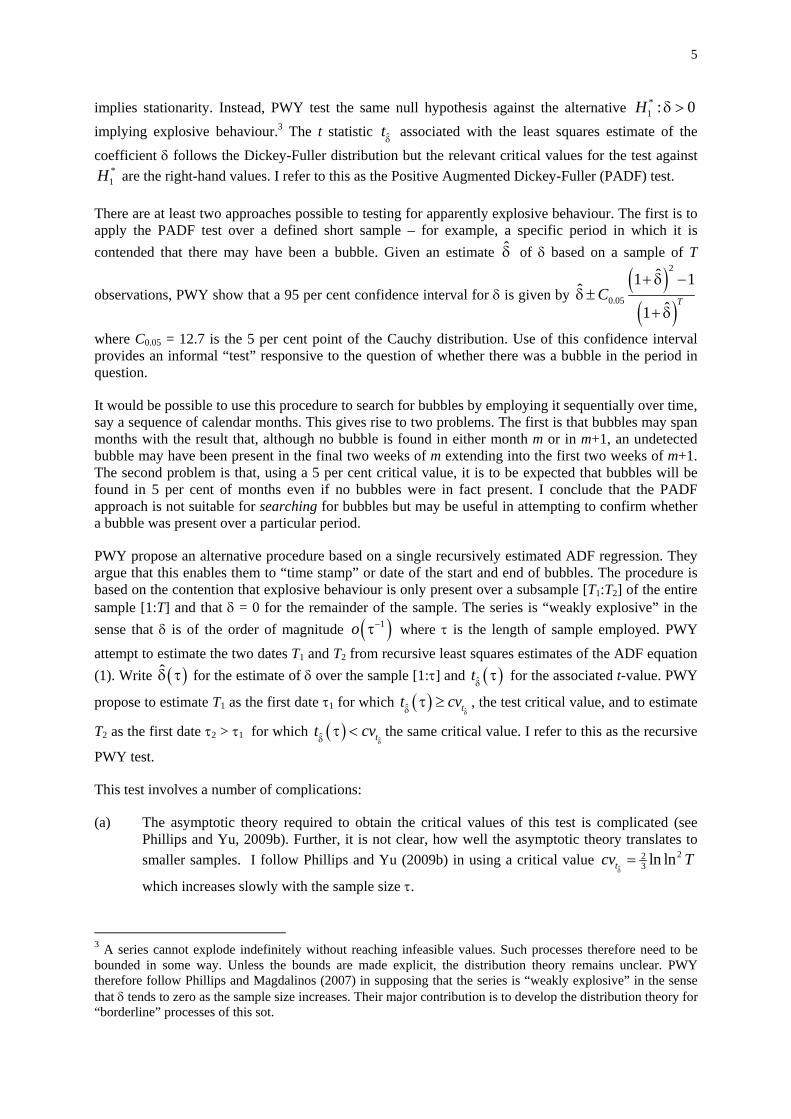
that a bubble must persist for three months to qualify. Figures 1–7 graph the ˆtδ test statistics (with the

test critical value as the smooth dashed line).

-3.0

-2.5

-2.0

-1.5

-1.0

-0.5

0.0

0.5

1.0

1.5

Jan-2001

Jan-2002

Jan-2003

Jan-2004

Jan-2005

Jan-2006

Jan-2007

Jan-2008

Jan-2009

Figure 1Monthly PWY recursive ADF(1) t statistics,

WTI crude oil

-5.0

-4.0

-3.0

-2.0

-1.0

0.0

1.0

2.0

Jan-2001

Jan-2002

Jan-2003

Jan-2004

Jan-2005

Jan-2006

Jan-2007

Jan-2008

Jan-2009

Figure 2Monthly PWY recursive ADF(1) t statistics,

aluminium

-3.0

-2.0

-1.0

0.0

1.0

2.0

3.0

Jan-2001

Jan-2002

Jan-2003

Jan-2004

Jan-2005

Jan-2006

Jan-2007

Jan-2008

Jan-2009

Figure 3Monthly PWY recursive ADF(1) t statistics,

copper

-2.0

-1.5

-1.0

-0.5

0.0

0.5

1.0

1.5

Jan-2001

Jan-2002

Jan-2003

Jan-2004

Jan-2005

Jan-2006

Jan-2007

Jan-2008

Jan-2009

Figure 4Monthly PWY recursive ADF(1) t statistics,

nickel

-5.0

-4.0

-3.0

-2.0

-1.0

0.0

1.0

2.0

Jan-2001

Jan-2002

Jan-2003

Jan-2004

Jan-2005

Jan-2006

Jan-2007

Jan-2008

Jan-2009

Figure 5Monthly PWY recursive ADF(1) t statistics,

corn

-3.5-3.0-2.5-2.0-1.5-1.0-0.50.00.51.01.5

Jan-2001

Jan-2002

Jan-2003

Jan-2004

Jan-2005

Jan-2006

Jan-2007

Jan-2008

Jan-2009

Figure 6Monthly PWY recursive ADF(1) t statistics,

soybeans

8

These estimates indicate a single bubble period – for copper over the eight months February to October 2006 (see figure 3). On a monthly average basis, cash copper rose steadily from $3,241/ton in May 2005 to a peak of $8,059/ton in May 2006. Note that the bubble is dated around the peak and not on the ascent itself (see figure 8). The post-bubble sample (November 2006 to June 2009) fails to show evidence of a second bubble, but this may only reflect the small number of remaining observations.6

For each of aluminium (figure 2) and nickel (figure 4), the procedure generates a t statistic in excess of the critical value for two isolated months – May 2006 and April 2007 respectively. Contrary to the results presented in Phillips and Yu (2009a), who used data from January 1990, I find no evidence for a bubble in the WTI oil price (see figure 1). This suggests that results may be sensitive to sample start data. There is little evidence for bubble behaviour in grains prices (see figures 5–7) although the wheat ADF t statistic does come very close to its critical vale in February and March 2008 – the time of the food price spike which von Braun and Torero (2009) claimed had speculative origin.

Turning to daily data, I consider the same seven commodities but now use daily closing prices over the sample 3 January 2006 to 31 December 2008 for crude oil and the three grains (753 and 755 observations respectively on account of

differences in holidays) and the longer sample 4 January 2000 to 31 December 2008 for the three non-ferrous metals, reflecting the earlier start of the metals boom (2271 observations). For crude oil and the three grains, I use closing prices for the first nearby month rather than for the delivery month to avoid illiquidity and other problems as contract maturity approaches. I roll contracts on the first day of the final month of trading. For the same reason, I use three month LME metals and not cash settlement prices.7 The tests again adopt an ADF(1) specification. I adopt the rule that a bubble must persist for ten working days if it is to count as economically interesting.

Table 1 summarizes the test statistics which are graphed in figures 9–15. I divide the seven commodities into three groups:

(i) The first group consists just of copper which stands out with three clear bubbles identified in 2004, 2006 and 2008 respectively. The third of these bubbles, which is associated with rapidly falling prices, spans the end of the sample. The 2006 bubble, which correspond with that

6 The t statistic graphed in figure 3 is that estimated over the entire sample. 7 The roll issue does not arise with LME prices since each day effectively corresponds with a different contract. My rolling convention implies that my CBOT and NYMEX “first nearby” will correspond to the second position in more normal parlance for all but the final days of the month.

-3.0

-2.5

-2.0

-1.5

-1.0

-0.5

0.0

0.5

1.0

1.5

Jan-2001

Jan-2002

Jan-2003

Jan-2004

Jan-2005

Jan-2006

Jan-2007

Jan-2008

Jan-2009

Figure 7Monthly PWY recursive ADF(1) t statistics,

wheat

0

1 000

2 000

3 000

4 000

5 000

6 000

7 000

8 000

9 000

10 000

Jan-1999

Jan-2000

Jan-2001

Jan-2002

Jan-2003

Jan-2004

Jan-2005

Jan-2006

Jan-2007

Jan-2008

Jan-2009

Figure 8Copper bubble (bold), monthly data

($/ton)

9

identified in the monthly data, is the only completely unproblematic case in that the estimated bubble period does not contain any holes.

(ii) The second group consists of crude oil, nickel and soybeans. A bubble is identified in the soybean market, in this case at the start of 2008, while bubbles are not found for crude oil or nickel. Nevertheless, all three outcomes are marginal and would be altered by small changes in the test critical values. The soybeans date-stamping is problematic since the estimated bubble period contains a 10 day hole. Strict application of the criteria set out in section III would require this bubble to be classified as a much shorter 16 day bubble terminating at the start of the hole. Crude oil presents similar test outcomes to soybeans but the ADF t statistic exceeds its critical value for fewer days and for a maximal duration of just seven days. Despite the similarities of the test outcomes, no bubble is identified. Nickel also shares characteristics with crude oil and soybeans but here there are no days in which the ADF t statistic exceeds its critical value despite being very close for a long period in 2007.

(iii) The remaining group consists of aluminium, corn and wheat. Here the test outcomes show clearly that there was no bubble. This is most clear in the case of corn where the ADF t statistic never approaches its critical value. In aluminium and wheat, the critical value is exceeded for a small number of days but not for long enough to identify a bubble period.

Table 1

BUBBLE TEST STATISTICS, DAILY DATA

# days with

ˆˆδδ tt cv≥

Longest

continuous period (days)

Max.

δ̂t

δ̂tcv

Date

Crude oil 21 7 1.68 1.41 3 July 2008

Aluminium 4 4 2.25 1.49 11 May 2006

Copper (2004) 51 26 2.30 1.46 1 March 2004

Copper (2006) 41 41 4.00 1.49 12 May 2006

Copper (2008) 15 12 1.96 1.52 24 December 2008

Nickel 0 - 1.47 1.50 5 April 2007

Corn 0 - 0.90 1.31 1 December 2006

Soybeans 37 17 2.39 1.40 3 March 2008

Wheat 6 4 1.59 1.38 1 October 2007

Note: The table reports the number of days in which the ADF t statistic exceeds its critical value, the maximum number of days for which it did so continuously, the maximal value of the statistic, the critical value for that sample and the date of the maximum.

10

-2.5

-2.0

-1.5

-1.0

-0.5

0.0

0.5

1.0

1.5

2.0

Apr-2006

Aug-2006

Dec-2006

Apr-2007

Aug-2007

Dec-2007

Apr-2008

Aug-2008

Dec-2008

Figure 9PWY recursive ADF(1) t statistics,

WTI crude oil, daily data

-3.0

-2.0

-1.0

0.0

1.0

2.0

3.0

Jan-2001

Jan-2002

Jan-2003

Jan-2004

Jan-2005

Jan-2006

Jan-2007

Jan-2008

Figure 10PWY recursive ADF(1) t statistics,

aluminium, daily data

-4.0

-3.0

-2.0

-1.0

0.0

1.0

2.0

3.0

4.0

5.0

Jan-2001

Jan-2002

Jan-2003

Jan-2004

Jan-2005

Jan-2006

Jan-2007

Jan-2008

Figure 11PWY recursive ADF(1) t statistics,

copper, daily data

-2.0

-1.5

-1.0

-0.5

0.0

0.5

1.0

1.5

2.0

Jan-2001

Jan-2002

Jan-2003

Jan-2004

Jan-2005

Jan-2006

Jan-2007

Jan-2008

Figure 12PWY recursive ADF(1) t statistics,

nickel, daily data

-3.0

-2.5

-2.0

-1.5

-1.0

-0.5

0.0

0.5

1.0

1.5

2.0

Apr-2006 Oct-2006 Apr-2007 Oct-2007 Apr-2008 Oct-2008

Figure 13PWY recursive ADF(1) t statistics,

corn, daily data

-5.0

-4.0

-3.0

-2.0

-1.0

0.0

1.0

2.0

3.0

Apr-2006 Oct-2006 Apr-2007 Oct-2007 Apr-2008 Oct-2008

Figure 14PWY recursive ADF(1) t statistics,

soybeans, daily data

11

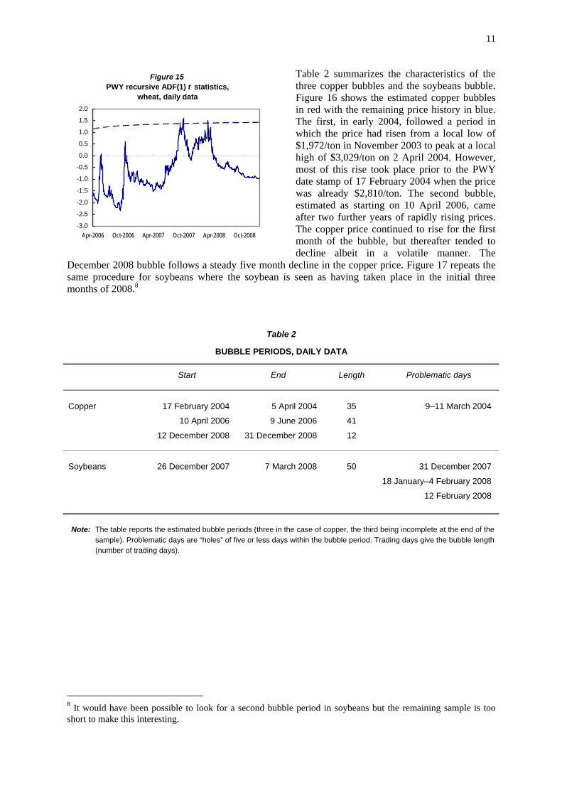
Table 2 summarizes the characteristics of the three copper bubbles and the soybeans bubble. Figure 16 shows the estimated copper bubbles in red with the remaining price history in blue. The first, in early 2004, followed a period in which the price had risen from a local low of $1,972/ton in November 2003 to peak at a local high of $3,029/ton on 2 April 2004. However, most of this rise took place prior to the PWY date stamp of 17 February 2004 when the price was already $2,810/ton. The second bubble, estimated as starting on 10 April 2006, came after two further years of rapidly rising prices. The copper price continued to rise for the first month of the bubble, but thereafter tended to decline albeit in a volatile manner. The

December 2008 bubble follows a steady five month decline in the copper price. Figure 17 repeats the same procedure for soybeans where the soybean is seen as having taken place in the initial three months of 2008.8

Table 2

BUBBLE PERIODS, DAILY DATA

Start End Length Problematic days

17 February 2004 5 April 2004 35 9–11 March 2004

10 April 2006 9 June 2006 41

Copper

12 December 2008 31 December 2008 12

Soybeans 26 December 2007 7 March 2008 50 31 December 2007

18 January–4 February 2008

12 February 2008

Note: The table reports the estimated bubble periods (three in the case of copper, the third being incomplete at the end of the sample). Problematic days are “holes” of five or less days within the bubble period. Trading days give the bubble length (number of trading days).

8 It would have been possible to look for a second bubble period in soybeans but the remaining sample is too short to make this interesting.

-3.0

-2.5

-2.0

-1.5

-1.0

-0.5

0.0

0.5

1.0

1.5

2.0

Apr-2006 Oct-2006 Apr-2007 Oct-2007 Apr-2008 Oct-2008

Figure 15PWY recursive ADF(1) t statistics,

wheat, daily data

12

0

1 000

2 000

3 000

4 000

5 000

6 000

7 000

8 000

9 000

Jan-2000

Jan-2001

Jan-2002

Jan-2003

Jan-2004

Jan-2005

Jan-2006

Jan-2007

Jan-2008

Figure 16LME copper "bubble periods", daily data

($/ton)

0

200

400

600

800

1 000

1 200

1 400

1 600

1 800

Jan-2006

May-2006

Sep-2006

Jan-2007

May-2007

Sep-2007

Jan-2008

May-2008

Sep-2008

Figure 17The soybean "bubble periods", daily data

($/bshl)

V. THE INTERPRETATION OF BUBBLE TESTS

These estimates generate both methodological and substantive questions. The methodological issues relate to the interpretation of the test outcomes and the differences between the daily and monthly estimates. The substantive issues relate to the extent to which important primary commodity prices were divorced from fundamental values over the initial decade of this century. I look at the methodological issues first.

PWY wish to interpret the start and end dates as the dates at which bubble periods started and ended. This interpretation may be mistaken. The start date is the first date at which, going forward, one can be confident that the price process has a root in excess of unity. That finding will necessarily be based on data from the preceding days (or periods) and will therefore come sometime after the start of the explosive period. This is apparent in all three copper bubbles (see figure 16). The copper futures price had been rising for a full year prior to the estimated start date of the 2004 bubble and for more than a year prior to the estimated start of the 2006 bubble. It had been falling for more than three months prior to the estimated start of the (negative) 2008 bubble. Similarly, the estimated end date will be based on data from days in which the price process has been non-explosive. It will also come after the end of an actual bubble. Significant ADF test statistics may therefore be confidently taken as indicating that there have been bubble episodes, but, contrary to the claims made by PWY, they should probably not be taken as accurate estimates of bubble dates.

If the price was indeed weakly explosive in the estimated bubble periods, this should be clear from estimating a standard ADF equation over the period in question. The results of this exercise are reported in table 3. In all four cases, the ADF(1) t statistics are negative over the estimated bubble periods, indicating a departure towards stationarity. In the case of the 2004 copper bubble, the statistic would allow rejection of the null of non-stationarity against the alternative of stationarity. By contrast, three of the four ADF(1) t statistics relating to the pre-bubble periods are positive In these three cases, I also report the 95 per cent (Cauchy-based) confidence interval for δ. These intervals are wide and fail to exclude the possibility that the process is non-explosive.

The results reported in table 3 underline the contention that the recursive PWY procedure should be seen as estimating the dates at which the observer can be sure that a bubble process respectively had been taking place and had been terminated and not dating the start and end of the bubble itself. Thus, in the case of copper, it would have been correct on 10 April 2006 to conclude that, with 95 per cent probability, the LME three months futures price was following a bubble process and on 9 June 2006 it would have been correct to conclude that, with 95 per cent probability, the bubble had ended.

13

Table 3 ADF STATISTICS DURING AND PRIOR TO THE ESTIMATED BUBBLE PERIODS

Pre-bubble period

Length (days) ADF(1)

ADF(1) δ̂ 95 per cent c.i.

Copper (2004) 35 - 3.35 0.70 0.030 - 0.229 0.289 Copper (2006) 41 - 2.32 1.43 0.070 - 0.044 0.185 Copper (2008) 12 - 1.32 - 1.05 - 0.216

Soybeans 50 - 1.34 0.09 0.021 - 0.170 0.211

Note: The table gives ADF(1) statistics for the logarithmic prices over the estimated bubble (including the estimated start and end dates), and also for the n days preceding the bubble (including the estimated bubble start date) where n is equal to the number of days in the estimated bubble. The final columns give the estimated δ̂ coefficient and, in the case of a positive estimate, the 95 per

cent implied confidence interval for δ.

The second methodological issue arises out of the contrast between results obtained for the same commodities at the monthly and the daily frequency summarized in tables 1 and 2 respectively. Of the four bubbles identified using daily data, only the 2006 copper bubble was found using monthly data. The ten day requirement is arbitrary, but is sensible if one interprets the recursive PWY test as dating bubbles. It makes less sense on the alternative interpretation that the test identifies periods when one can be confident that there has been a bubble. This reinterpretation goes some way to resolving the problems, highlighted in table 1, associated with isolated bubble signals and holes. If the recursive PWY procedure is indeed backward looking and does not date-stamp the bubbles themselves, these days or groups of days cease to be problematic. Given that it is notoriously difficult even for industry experts to determine whether a price is or is not fundamentally-based, we should not be surprised that econometric methods fail to give clear cut answers in marginal cases. On this basis, we might wish to reinterpret the results obtained from the daily recursive PWY tests as implying that bubbles quite possibly were present in crude oil during the first half of 2008 and in nickel during the first three months of 2007, in addition to the clearer cases of copper and soybeans already discussed.

The problem is different in the case of soybeans where the tests using daily data find a bubble over the December 2007–March 2008 but this is not apparent using monthly data. Investigation reveals that this difference in results arises out of the different start dates for the sample. If the monthly sample is reduced to the 56 months (January 2005–June 2009), the recursive PWY test critical value is exceeded for the months, January and February 2008, consistently with the daily test results. This is problematic for the procedure since it suggests the paradoxical conclusion that the bubbles may be more difficult to detect if set against a long backdrop of non-explosive behaviour.

Substantively, it does seem reasonable to conclude that oil and some non-ferrous metals prices have exhibited explosive behaviour over at least sub-periods of the recent decade. This is most evidently the case in copper. These bubbles are consistent with explanations in terms of extrapolative behaviour, perhaps on the past of CTAs and other trend-following speculators. However, there are also other possible interpretations. First, the “market fundamental” may have explosive over these periods. Crude oil and non-ferrous metals are all industrial commodities and market opinion ascribes recent high prices to rapid growth in Asia, particularly Chinese demand. Second, even if demand growth was not explosive, it is possible that market perceptions of these possibilities grew in an extrapolative manner. Third, rapid demand growth brings markets close to stockout. This results in a nonlinear relationship between price and the fundamental which might appear as explosive behaviour (see Wright and Williams, 1991 and Deaton and Laroque, 1992). Perhaps, more than one of these factors was operative with a resulting compounding effect. Finally, the history of the copper market, both historically and in

14

the 1990s (see Tarring, 1997), indicates that lone should not entirely rule out the possibility of manipulative Ponzi-type behaviour.

VI. FUTURES SPECULATION AND FUTURES INVESTMENT

In the remainder of the paper, I consider the effects of index investment, introduced above in section II, on commodity futures prices. Transactors in futures markets are generally classified as either hedgers or speculators and the exchanges are seen as transferring price exposure from the hedgers to speculators in exchange for a risk premium. Speculators take a view, either on the basis of information or through the use of more or less sophisticated trend-spotting procedures, on the prospects of the particular commodities in which they take positions.

The CFTC requires brokers to report all positions held by traders with positions exceeding a specified size, and also to report the aggregate of all smaller (“non-reporting”) positions. These positions are published in anonymous and summary form in the weekly CFTC Commitments of Traders (COT) reports. The CFTC classifies reporting traders as either “commercial” or “non-commercial” depending whether or not they have a commercial interest in the underlying physical commodity. Commentators, both academic and in the futures industry, routinely interpret commercial positions as hedges, non-commercial positions as large speculative positions and non-reporting positions as small speculative positions (see Edwards and Ma, 1992: 15–17). Upperman (2006) provides a guide to trading on the basis of the COT reports.

In what follows, I distinguish between speculation in commodity futures and investments in commodities which use futures contracts, directly or indirectly, as investment vehicles. The distinction depends on the motivation of the actor in question. A speculator takes a view about the likely returns on a particular commodity future, say in crude oil, in relation to the riskiness of that return and takes a positive, zero or negative position accordingly. An investor takes a view on the effects of adding a commodity component to an investment portfolio on the basis of the risk-return characteristics of the overall portfolio. In practice, commodity investors take long positions and tend to track one of two widely quoted commodity futures indices. For this reason, they are generally referred to as “index investors”. Index investments are most commonly implemented through swap structures negotiated through a number of banks and brokers referred to as “index providers”.

It is widely perceived that, as the consequence of the increased diversity of futures actors and the increased complexity of their activities, the COT data may fail to fully represent futures market activity. Many institutions reporting positions as hedges, and which are therefore classified as commercial, are held by index providers to offset swap positions which, if held directly as commodity futures, would have counted as non-commercial. As the CFTC has itself noted “… trading practices have evolved to such an extent that, today, a significant proportion of long-side open interest in a number of major physical commodity futures contracts is held by so-called non-traditional hedgers (e.g. swap dealers) … This has raised questions as to whether COT report can reliably be used to assess overall futures activity …” (CFTC, 2006: 2).

The driving rationale of investment in commodity futures is that commodities may be considered as a distinct “asset class”, and seen in this light, have favourable risk-return characteristics. The claim that commodities form a distinct asset class, analogous with the equity, fixed interest and real estate asset classes, supposes that the class is fairly homogeneous so that it may be spanned by a small number of representative positions. Specifically, this requires that the class have a unique risk premium which is not replicable by combining other asset classes (see Scherer and He, 2008). Given this premise, the claim that commodities form an asset class which is interesting to investors relies on their exhibiting a sufficiently high excess return and sufficiently low correlations with other asset classes such that, when added to portfolio, the overall risk-return characteristics of the portfolio improve (see Bodie and Rosansky, 1980; Jaffee, 1989; Gorton and Rouwenhorst, 2006 and for a summary, Woodward, 2008).

15

Figure 18 Commodity composition, S&P GSCI and DJ-UBS commodity indices, September 2008

S&P GSCI

Livestock3.5%

Non-ferrous metals6.5%

Softs2.6%

Grains and vegetable

oils9.9%

Precious metals1.8%

Energy75.6%

DJ-UBS commodity indices

Energy33.0%

Precious metals10.1%

Grains and vegetable

oils20.8%

Softs8.7%

Non-ferrous metals20.0%

Livestock7.4%

Index funds set out to replicate a particular commodity futures index in the same way that equity tracking funds aim to replicate the returns on an equities index, such as the S&P500 or the FTSE100. The most widely followed commodity futures indices are the S&P GSCI and the DJ-UBS index (previously the DJ-AIG index). The S&P GSCI is weighted in relation to world production of the commodity averaged over the previous five years.9 These are quantity weights and hence imply that the higher the price of the commodity future, the greater its share in the S&P GSCI. Recent high energy prices imply a very large energy weighting – 71 per cent in September 2008. The DJ-UBS index weights the different commodities primarily in terms of the liquidity of the futures contracts (i.e. futures volume and open interest), but in addition considers production. Averaging is again over five years. Importantly, the DJ-AIG index also aims for diversification and limits the share of any one commodity group to one third of the total. The September 2008 energy share fell just short of this limit.10 September 2008 weightings of these two indices are charted in figure 18.

The sums of money invested by this third group of commodity investors may be very substantial. Using official non-public information, the CFTC estimated the notional value of positions held in index-related investments at the end of December 2007 as $146 billion ($118 billion on the United States exchanges) rising to $200 billion at the end of June 2008 ($161 billion on the United States exchanges), (see CFTC, 2008). Table 4 summarizes these data for the eleven commodities covered in the CFTC’s special call on commodity swap and index providers, reported in CFTC (2008).11 Of the $161 billion of commodity index business in the United States markets at the end of 30 June 2008, approximately 24 per cent was held by index funds, 42 per cent by institutional investors, 9 per cent by sovereign wealth funds and the remaining 25 per cent by other traders (CFTC, 2008). The table also gives the estimated shares of net index positions in total open interest. These average 26–27 per cent, but are much higher for copper, crude oil, wheat, live cattle and lean hogs.

In what follows, I report an estimate of the quantum of index investment across the range of commodity futures over the period 2006–2008. A large literature relates changes in futures prices to

9 http://www2.goldmansachs.com/gsci/#passive. 10 http://www.djindexes.com/mdsidx/index.cfm?event=showAigIntro. 11 Twelve contracts since wheat is traded on both the Chicago Board of Trade and the Kansas City Board of Trade.

16

the net positions of non-commercial traders, often identified as “large speculators”, identified in the CFTC’s weekly Commitments of Traders (COT) reports. Commercial traders (“hedgers”), who are the counterparts of the non-commercials, are interpreted as not taking a view on prices. However, the increased complexity of the modern futures industry implies that the division of futures positions into commercial and non-commercial categories may have become arbitrary and that the standard COT net non-commercial positions variable is likely to be less informative in the current environment than it may previously have been.

Table 4

VALUES AND SHARES OF INDEX-RELATED INVESTMENTS

31 December 2007 30 June 2008

$bn Share

(Per cent)

$bn Share

(Per cent)

Crude oil 39.1 31.1 51.0 26.6 Gasoline 4.5 22.9 8.0 23.9 Heating oil 7.8 34.8 10.0 34.5 Natural gas 10.8 16.8 17.0 14.7

Copper 2.8 49.9 4.4 41.7 Gold 7.3 15.9 9.0 22.7 Silver 1.8 15.5 2.3 20.1

Corn 7.6 25.8 13.1 27.4 Soybeans 8.7 26.1 10.9 20.8 Soybean oil 2.1 24.8 2.6 21.7 Wheat 9.3 38.2 9.7 41.9

Cocoa 0.4 11.3 0.8 14.1 Coffee 2.2 26.0 3.1 25.6 Cotton 2.6 33.0 2.9 21.5 Sugar 3.2 29.0 4.9 31.1

Feeder cattle 0.4 23.2 0.6 30.7 Live cattle 4.5 48.4 6.5 41.8 Lean hogs 2.1 43.6 3.2 40.6

Other United States markets 0.7 1.4 Total (United States markets) 117.9 26.8 161.5 25.8 Non-United States markets 28.1 38.4 Overall total 146.0 199.9

Source: Columns 1 and 3 CFTC (2008) valued at front position closing prices; columns 2 and 4, CFTC, Commitment of Traders reports. The wheat figures aggregate positions on the Chicago Board of Trade and the Kansas City Board of Trade. Open interest is valued at the closing price of the front contract. The aggregate share relates topositions on the United States exchanges for the listed commodities. Except in the final two rows, figures relateonly to positions held on the United States exchanges.

Responding to these concerns, the CFTC has, starting in January 2006, issued a supplementary report for twelve agricultural futures markets which distinguish positions held by institutions identified as index providers. However, they did not choose to provide this additional information for energy and metals futures at that time, on the grounds that offsetting may involve taking positions on non-United

17

States exchanges and because many swap dealers in metals and energy futures have physical activities on their own account making it difficult to separate hedging from speculative activities (see CFTC, 2006).

I have used this information in the CFTC’s COT Supplementary Reports to construct a quantum index of total net index-related futures positions on the United States agricultural markets from the start of 2006.12 The resulting “Corazzolla index” is graphed in figure 19.13 The index rose sharply in the first five months of 2006 but was then broadly flat until the final months of 2007. A second sharp rise brought it to a peak at the end of April 2008. It then fell steadily (precipitately in September and October 2008) to reach a low in February 2009, at which point it was slightly beneath its value at 2006. There has subsequently been a modest recovery.

The Corazzolla index was calculated using data on index provider positions on agricultural futures markets, which is the only information that CFTC made available on a consistent basis

over the period of interest. This poses the question of the extent to which this index may also be taken as measuring total index provider positions. Since index composition only changes slowly (DJ-UBS) or not at all (S&P-GSCI) one might suppose the agricultural index to be representative of total index positions. From table 2, we find that index positions on the United States agricultural futures markets accounted for 36.6 per cent of total index provider positions on the United States exchanges on 31 December 2007 and 34.9 per cent on 30 June 2008. Weekly variations in this share are, however, more important than its trend evolution. Two factors indicate that the index may be less than fully representative of the total:

(a) Index providers now offer a variety of sub-indices with the result that index investment has assumed a greater judgemental component;

(b) The CFTC figures relate to the futures positions taken by the index providers to offset their index exposure. Offsetting may be discretionary, in particular in relation to timing, even if index investment is not.

It is therefore difficult to make an a priori judgement on the representativeness of the Corazzolla index for total index positions. However, one might suggest that the test of the adequacy of the index is its ability to explain movements in commodity prices. This is the subject of section VII.

12 Data are taken from the CFTC’s Supplementary Commitments of Traders Reports. The markets covered are: corn (maize), soybeans, soybean oil and soft wheat (Chicago Board of Trade), hard wheat (Kansas City Board of Trade), cocoa, coffee, cotton and sugar (New York Board of Trade) and feeder cattle, lean hogs and live cattle (Chicago Mercantile Exchange). Positions are measured in contracts. The index uses value weights as of 31/12/2007 to weight the net position (in contracts) on each exchange. 13 The index is named for Elena Corazzolla who performed the calculations as part of her 2009 Trento laurea dissertation.

75

100

125

150

175

200

225

Jan-2006 Jul-2006 Jan-2007 Jul-2007 Jan-2008 Jul-2008 Jan-2009

Figure 19Quantum index of net positions taken by index providers on United States

agricultural futures markets(Index numbers, 03/01/2006 = 100)

18

VII. INDEX INVESTMENT IN COMMODITY FUTURES MARKETS

In this section, I explore the results obtained by relating the Corazzolla index, discussed in section VI, to change in commodity prices over 2006–2008. The econometric methodology employed in testing for the effects of index investment, or any other set of futures markets positions, is standard. Granger-causality analysis may be employed to relate futures returns at any specified level of temporal aggregation (daily, weekly, monthly, etc.) to changes in positions. Consider the first equation of a

bivariate VAR(p) (i.e. a pth order Vector AutoRegression) linking futures returns ln tfΔ to changes

in positions txΔ

1 1

ln lnp p

t j t j j t j tj j

f f x u− −= =

Δ = α + β Δ + γ Δ +∑ ∑ (2)

The Granger-causality test (strictly a non-causality test) is the standard Wald test

0 1: 0pH γ = = γ =L against the alternative of its negation. The order p of the VAR is determined by

testing down from a general specification employing a large value of p. Note that equation (2)

excludes the current period value txΔ so, while on the one hand there are no simultaneity issues which

complicate inference, on the other hand. The test is silent with respect to contemporaneous causation. A favourable result from a Granger causality test establishes a prima facie case that there is a causal relationship between the two variables.

Table 5 gives the results of Granger-causality tests linking weekly logarithmic changes in the Corazzolla measure of net index positions on the United States agricultural futures markets and logarithmic changes in the seven commodity futures prices already considered in section V above. The first two columns of the table ask whether the changes in the futures prices Granger-cause changes in the Corazzolla index while the final two columns reverse the question and ask whether index positions Granger-cause changes in the futures prices. In columns 1 and 3, I take p = 3 (tested down from an initial value of p = 6) while in column 4, I reduce to p = 2, except in the case of copper, where this reduction is rejected by the Wald statistic (not reported). A distributed lag of length 3 is always required in explaining changes in the Corazzolla index, but it is possible to reduce the length of the futures price distributed lag to one (column 2).

Looking initially at the first two columns, we see that changes in the Corazzolla index are Granger-caused by changes in the three agricultural futures prices (most evidently, that of corn), but there is no evidence of a Granger-causal link either from the crude oil price or from the non-ferrous metals prices. This is consistent with the view that the Corazzolla index does indeed represent positions in agricultural futures markets and may not be representative of positions in energy and metals markets. However, the test results reported in columns 3 and 4 tell a different story: changes in the Corazzolla index Granger-cause changes in crude oil, aluminium and copper futures prices as well as changes in corn futures prices but they do not Granger-cause changes in wheat or soybean futures prices. Importantly, the fact that the index does have predictive power for energy and non-ferrous metals markets demonstrates both that it is to some extent representative of index positions in non-agricultural futures markets and that the changes in these positions have been associated with some price impact.

Granger-causality tests establish the presence of a causal link (at the specified level of confidence) between the posited causal variable and the variable of interest, but do not imply that this link is direct. Specifically, there is the worry that the variable of interest and the posited causal variable may be jointly caused by some third variable, may be intermediated by such a variable or may simply exhibit a high sample correlation with this third variable. There are three variables that cause particular concern: the United States dollar exchange rate; levels of economic activity and the physical supply and demand conditions in the markets in question.

19

Table 5 GRANGER-CAUSALITY TESTS

Null hypothesis “Row variable Granger-non-causes Net Index Positions”

“Net Index Positions Granger-non-cause row variable”

Model ADL(3,3) ADL(3,1) ADL(3,3) ADL(2,2) Statistic F3,159 F1,161 F3,159 F2,161

Crude oil (NYMEX, WTI)

0.82 [48.6%]

0.19 [66.5%]

4.58 [0.52%]

7.99 [0.01%]

Aluminium (LME, 3 month)

0.65 [58.7%]

0.17 [67.8%]

4.98 [0.03%]

7.89 [0.01%]

Copper (LME, 3 month)

0.63 [59.4%]

0.22 [64.1%]

2.92 [3.54%]

-

Nickel (LME, 3 month)

0.04 [84.5%]

0.35 [55.4%]

1.59 [19.4%]

2.68 [7.16%]

Wheat (CBOT, 1st nearby)

2.16 [9.44%]

5.31 [2.25%]

1.82 [14.2%]

1.49 [22.9%]

Corn (CBOT, 1st nearby)

2.94 [3.50%]

7.87 [0.06%]

2.13 [9.85%]

4.21 [1.65%]

Soybeans (CBOT, 1st nearby)

2.02 [11.3%]

5.74 [1.77%]

1.38 [25.2%]

1.92 [15.0%]

Dollar exchange rate index 2.57 [5.62%]

4.53 [3.49%]

2.88 [3.80%]

-

Equity index (average S&P and Hang-Seng)

2.79 [4.24%]

- 1.81 [14.7%]

2.86 [6.01%]

Note: The table reports Granger-non-causality tests in relation to logarithmic changes in the Net Index Positions variable, defined in the text, and logarithmic changes in the seven futures prices under consideration and also an index of the value of the United States dollar. In columns 2 and 4, the tests are performed on restricted versions of the ADL(3,3). For copper and the exchange rate index, no test is reported in column 4 since the implied restrictions are rejected. Data are weekly from 31/01/2006 (columns 1 to 3) or 24/01/2006 (column 4) to 31/03/2009. Tail probabilities are given parenthetically. Bold face indicates rejection of the null hypothesis of Granger-non-causality at the 5 per cent level (i.e. “acceptance” of Granger-causality).

I have constructed an index of the value of the United States dollar against a basket of major currencies14 for conformable dates with those of the COT Supplementary Reports. This index is graphed in figure 20 from which it is clear that the movements are inverse those of the Corazzolla net index positions index. The correlation between the two indices is – 0.76 in levels and – 0.29 in differences. The penultimate row of table 5 reports that changes in the United States dollar exchange rate Granger-cause changes in index positions, consistent with the view that dollar-based investors take positions in commodity index investments to protect themselves against possible dollar depreciation, and, more surprisingly, that index investments Granger-cause changes in the value of the dollar.

14 The Eurozone, Japan, United Kingdom, Switzerland, Australia and Canada with weights 4:4:1:1:1:1. Data source: European Central Bank.

20

Indices of economic activity are not available at higher than monthly frequencies. It would be possible to interpolate monthly indices to a weekly or daily basis but such a procedure runs the danger of allowing commodity futures returns to depend on measures of activity relating to the future. A further problem is that commodity futures prices reflect anticipated level of economic activity and hence tend to lead actual changes in activity. As an alternative, I include returns on stock exchange indices, which are available at the weekly frequency and which also reflect growth expectations rather than growth itself. Specifically, I look at the returns on the Standard and Poors 500 index of the United States equity prices ΔlnSPt and, to reflect the importance of Chinese growth, returns on the

Hang Seng index ΔlnHSt. Use of the average equity return [ ]12ln ln lnt t tEQ SP HSΔ = Δ + Δ appears

generally acceptable in place of the two original returns. The final row of table 5 shows that changes in equities prices Granger-cause changes in index-based investments by not vice versa.

Market analysts typically analyze commodity price changes primarily in terms of the supply-demand balance for the commodity. To the extent that these fundamentals are correlated across commodities, they may also be correlated with index investments. If this is the case, index investors, along perhaps with traditional speculators, would be the transmission mechanism whereby information on market fundamentals become impounded in futures prices. In a number of markets, exchange warehouse stocks provide a convenient measure of the state of market fundamentals, although it is never clear how representative these stock levels are of total availability of the commodity. In practice, these variables do not contribute to the explanation of commodity returns once equity returns and index investment are included in the equations.

The second important qualification with regard to Granger-causality analysis is that it is silent with respect to contemporaneous correlation. This is important in the current context since both liquidity and information with all considerations suggest that index-based transactions, in common with all other futures market transactions, will impact prices at the time of the transaction. Granger-causality analysis will capture this impact only in so far as past value of index-based positions predict current changes in these positions. Test power may therefore be weak. At the same time, week-on-week changes in index-based positions may reflect price movements within the week in question (particularly since these are offsetting positions taken by the index providers) establishing the possibility of bidirectional causality.

The correlations between the contemporaneous price changes and change in the net index positions are high for crude oil (0.440), aluminium (0.535) and copper (0.456). The cross-plots are graphed in figures 21, 22 and 23 respectively. (The crude oil correlation rises to 0.501 if the post-Lehman week ending 23/09/2008 is omitted). The high correlations for these three commodities suggest that contemporaneous links cannot be ignored. This is in line with what one should expect on the basis of efficient markets theory. The correlations (not illustrated) for nickel and the three agricultural commodities are much lower (0.25 to 0.29).

75

85

95

105

Jan-2006 Jul-2006 Jan-2007 Jul-2007 Jan-2008 Jul-2008 Jan-2009

Figure 20Index of the value of the United States dollar

against a basket of currencies(Index numbers, 03/01/2006 = 100)

21

-20

-15

-10

-5

0

5

10

15

20

25

-8 -6 -4 -2 0 2 4 6

23/09//2008 r = 0.440

Figure 21Cross-plot, weekly changes in NYMEX WTI front contract against

change in net index positions, 10 January 2006–31 March 2009(Per cent)

-20

-15

-10

-5

0

5

10

15

20

25

-8 -6 -4 -2 0 2 4 6

r = 0.535

Figure 22Cross-plot, weekly changes in LME 3 month aluminium settlement price against

change in net index positions, 10 January 2006–31 March 2009(Per cent)

-20

-15

-10

-5

0

5

10

15

20

25

-8 -6 -4 -2 0 2 4 6

r = 0.456

Figure 23Cross-plot, weekly changes in LME 3 month copper settlement price against

change in net index positions, 10 January 2006–31 March 2009(Per cent)

22

I explore two approaches to analyzing the impact of changes in index positions on futures prices taking into account the contemporaneous interactions. In both cases, I also control for market fundamentals. In the first case, I suppose that all effects are contemporaneous, consistent with the Efficient Markets Hypothesis, and estimate equations of the form

ln ln lnj j j j jt t t tf NIP EQ uΔ = α +β Δ + γ Δ + (3)

where jtf is the jth futures price, NIPt is the Corazzolla index of net index positions, ln tEQΔ is the

equity returns index defined above and measured contemporaneously with the futures prices. The seven equations are estimated by instrumental variables (IV) taking the change in net index positions

ln tNIPΔ , the change in equities prices ln tEQΔ and the change in warehouse stocks to be either

endogenous or measured with error. The instrumental variables are implied by the Granger-causality tests reported in table 5: three lags each of ΔlnNIP, three lags each of ΔlnNIP, ΔlnEQ, ΔlnER and the VIX volatility index and the lagged returns on wheat, corn and soybean futures and the lagged returns on wheat, corn and soybean futures. Estimation results are reported in table 6.15

The β̂ coefficients of the change in net index positions are large for crude oil and the three non-

ferrous metals, although they are imprecisely determined. By contrast, the β̂ coefficients do not differ

significantly from zero for the three grains, although the failure to reject is marginal in the case of soybeans. Using the system 3SLS (Three Stage Least Squares) estimator, joint restriction of these three coefficients to zero is not rejected for the three grains but is rejected for the metals.16 It is notable that the Corazzolla index, constructed on the basis of agricultural futures markets, appears to explain movements in industrial commodity prices better than it does movements in agricultural prices. This lends support to the view that the Corazzolla index may be taken as representing total index-related investments, not just those in agriculture. On this view, the high coefficients for the non-agricultural commodities reflect the greater presence of these investments in energy and metals futures markets (see table 4).

The second approach I explore is based on the efficient markets view that only innovations should affect asset price returns. A standard methodology is that of regressing changes in futures prices on distributed lags of measures of trading activity (see, for example, Hasbrouck, 1991). Finance theory implies that these measures only be associate with a price impact to the extent that the trading activity conveys information into the market. Informed traders may attempt to disguise themselves as uninformed traders, or simply to hide behind the activities of uninformed traders. This may make it difficult for counterparties to accurately infer whether a particular trade is or is not informed. However, any price impact from uninformed trades should be transient.

15 I also explored inclusion of the contemporaneous change in the dollar exchange rate index ln tERΔ discussed

above and, for crude oil and the three metals, changes in deliverable stocks (Cushing for WTI, LME warehouses for the three metals). The coefficients of these variables were non statistically significant, although the exchange

rate coefficient was generally significant in the absence of the variable ln tEQΔ . This latter variable is also

dollar-denominated and so it is possible that exchange rate effects enter via this route. The restriction of the

coefficients of ln tSPΔ and ln tHSΔ to be equal is always satisfied. The results reported in table 6 are not

sensitive to relaxation of this constraint or inclusion of additional controls. 16 Since the equations contain the same regressors and use the same instrument set, unrestricted 3SLS gives the same estimates as the IV estimates reported in the first two columns of the table.

23

Table 6 INSTRUMENTAL VARIABLES ESTIMATES OF EQUATION (3)

Coefficient β̂ γ̂

Variable ln tNIPΔ ln tEQΔ Standard

error

Instrument validity χ2(13)

Joint significance

χ2(3)

Crude oil 0.882 (2.00)

1.326 (3.65)

5.25% 6.70 [91.7%]

Aluminium 0.851 (3.44)

0.511 (2.51)

2.94% 19.1 [12.0%]

Copper 1.078 (2.73)

0.968 (2.98)

4.70% 12.6 [38.3%]

Nickel 1.317 (2.61)

0.356 (0.86)

6.01% 19.0 [12.4%]

16.1 [0.1%]

Wheat 0.740 (1.61)

0.443 (1.46)

5.47% 9.72 [71.7%]

Corn 0.652 (1.47)

0.247 (0.68)

5.27% 17.6 [17.3%]

Soybeans 0.613 (1.90)

0.464 (1.74)

3.85% 17.0 [19.9%]

6.31 [9.76%]

Note: The table reports Instrumental Variables estimates of the return on the row j futures price ln jtfΔ on a constant

(coefficient α̂ not reported), and the three column variables (two for wheat, corn and soybeans) as specified in

equation (3) in the text. Both the net index positions ln tNIPΔ and the change in equity values ln tEQΔ are

treated as endogenous. The instruments are three lags each of ΔlnNIP, ΔlnEQ, ΔlnER and VIX and the lagged returns

on wheat, corn and soybean futures. The χ2(3) tests for joint significance test exclusion of ln tNIPΔ from the three

non-ferrous metals and grains equations respectively in the model estimated by 3SLS. Data are weekly from 31 January 2006 to 31 Mach 2009. Tail probabilities are in square “[.]” parentheses and t statistics in round “(.)” parentheses.

Illiquidity may counteract information considerations. In an order book trading system, such as that approximated by commodity futures markets, large transactions will inevitably push into the order book and hence have at least a transient price impact. If a market becomes unbalanced, as when index-based investment creates a predominance of buy-side interest, counterparties are likely to require an enhanced risk premium if they are to take on the off-setting short exposure. This can create a situation analogous to a speculative bubble in which potential counterparties are disinclined to take short positions in the knowledge that index-based buying may push prices to higher levels. In this way, the effects of index-based investment may become observationally equivalent to those of trend-following extrapolative expectations.

This discussion motivates examination of equations of the form

1

0 0

ˆ ˆlnp

j j j j j jt i t i i t i t

i if u− −

= =

Δ = α + β ε + γ ν +∑ ∑ (4)

24

where the ˆ tε are the residuals from the regression of ln tNIPΔ on the complete set of variables used

as instruments in the estimates reported in table 6 and the ˆ tν are the residuals from the regression of

ln tEQΔ on three lags of itself and three lags of the VIX volatility index.17

Estimation results are given in table 7. For the three grains, it is possible to set the entire equity return

distributed lag to zero (see bottom panel). The estimated lead coefficient β̂ on the net index

investment variable differs significantly from zero for all seven commodities, and in the case of the three grains, this is also true whether or not the equity index innovations are also included in the regression. In all seven cases, the sum of the estimated β coefficients exceeds the initial coefficient β0 although this sum is less precisely determined than the initial impact. The market efficiency condition (final column), which sets the coefficients of all the lagged innovations to zero, is rejected for crude oil, copper and wheat with only a marginal failure to reject in the case of aluminium. These results therefore both confirm the claim that index investment impacted the range of commodity futures prices and, at the same time, contradict a market illiquidity interpretation of the effects of index investment and instead are consistent with the view that these transactions convey information.

Overall, the Granger-causality tests reported in table 5 and the regression results reported in tables 6 and 7 confirm that index-based investment in commodity futures has a price impact, and that this impact is permanent. The Corazzolla measure of index-based investment, constructed from the CFTC’s Supplementary COT Reports, is based solely on data on positions in the United States agricultural futures markets. It is therefore remarkable that this measure explains movements in energy and metals futures prices better than it does movements in the agricultural futures prices themselves. It is known that index-based investments tend to concentrate in energy and metals markets and these results therefore encourage the contention that the Corazzolla index is representative of changes in the entire range of commodity futures markets.

The results appear to favour an informational explanation of the price impact of index-based investment over a liquidity-based explanation. This is despite the fact that, at least according to its proponents, index-based investment in commodities is motivated by portfolio diversification rather than informational considerations. This suggests that index-based investors may possess information on the likely prospects of the entire “commodity asset class” and that their transactions impound this information in the various futures prices entering the indices.

We can use the estimated price impacts from tables 6 and 7 to estimate the extent to which index investment may have raised commodity futures prices. I choose to use the estimates given in table 6 on the basis that these are robust endogeneity of the index investment variable. We may regard the net index investment ln NIPΔ and equity ln EQΔ variables in the table 6 equations as having been

generated within a Vector AutoRegression (VAR) structure in which the other variables are the instruments z in the equations. Provided the commodity price changes, which form the dependent variables in table 7, are strongly exogenous with respect to all these variables, we can perform counterfactual simulations of the commodity prices, holding the z variables constant, by setting to zero

the innovations ε̂ in ln NIPΔ , net of any contemporaneous impact from the innovations ν̂ in the

equity index ln EQΔ . (These innovations are precisely those which form the regressors in the

estimates presented in table 7).

17 A Wald block exogeneity test on the remaining nine variables in the equation for ln tNIPΔ indicated that

these could be dropped from this equation: F9,150 = 0.51 with tail probability of 86.7 per cent.

25

Table 7 INNOVATION REGRESSION RESULTS

Coefficient 0β̂

5

0

ˆj

j=β∑

0γ̂

5

0

ˆ jj=γ∑

Variable ˆ tε 5

ˆ ˆt t−ε εK

ˆ tν

5ˆ ˆ, ,t t−ν νK

R2 and Standard

error

Wald test

1 5 0γ = = γ =K

1 5 0β = = β =K

F10,152

Crude oil 1.182 (3.44)

3.283 (3.85)

0.425 (3.12)

0.766 (2.19)

0.298 4.86%

2.90 [0.24%]

Aluminium 0.931 (4.42)

1.837 (3.52)

0.112 (1.35)

0.353 (1.65)

0.243 2.97%

1.88 [5.22%]

Copper 1.059 (3.33)

3.377 (4.29)

0.216 (1.72)

0.314 (0.97)

0.224 4.49%

2.03 [3.35%]

Nickel 1.341 (3.10)

2.377 (2.22)

0.320 (1.87)

1.059 (2.40)

0.193 6.12%

1.73 [7.91%]

Wheat 0.776 (2.07)

2.981 (3.22)

0.076 (0.52)

- 0.064 (0.17)

0.176 5.29%

2.37 [1.25%]

Corn 1.042 (2.79)

1.483 (1.60)

0.116 (0.79)

0.571 (1.50)

0.143 5.29%

1.44 [16.8%]

Soybeans 0.777 (2.85)

1.555 (2.30)

0.148 (1.37)

0.535 (1.93)

0.168 3.85%

1.55 [12.6%]

F5,158

Wheat 0.905 (2.62)

3.107 (3.72)

- - 0.120 5.33%

3.28 [0.76%]

Corn 1.104 (3.32)

2.107 (2.54)

- - 0.111 5.28%

2.01 [7.96%]

Soybeans 0.849 (3.36)

2.117 (3.46)

- - 0.118 3.89%

2.06 [7.39%]

Note: The table reports OLS estimates of the return on the row j futures price ln jtfΔ on a constant (coefficient α̂ not

reported), a distributed lag of the innovations 5ˆ ˆt t−ε εK from the Net Index Positions equation, the log change in

the exchange rate index and the innovation in the log of warehouse stocks (not wheat, corn or soybeans). See equation (4). Data are weekly from 31/01/2006 to 31/03/2009. Tail probabilities are in square “[.]” parentheses and t statistics in round “(.)” parentheses.

The estimated price impacts are given in table 8. They are reported as annual averages and are proportional to the estimated β coefficients in table 6. The table also gives the maximum extent to which prices were increased. Figures 24–30 chart actual and counterfactual prices.

26

Table 8 ESTIMATED AVERAGE PRICE IMPACT

(Per cent)

Average impact

2006 2007 2008h1 2008h2

Maximum impact

Crude oil 8.2 4.9 23.7 7.3 28.6

Aluminium 5.9 3.5 17.0 5.2 20.6 Copper 7.5 4.5 21.6 6.6 26.0 Nickel 9.2 5.5 26.4 8.1 31.8

Wheat 5.2 3.1 14.8 4.5 17.9 Corn 4.6 2.7 13.0 4.0 15.8 Soybeans 4.3 2.5 12.3 3.8 14.8

Note: Estimated annual price impact of index-based investment in commodity futures based on the estimated coefficients in table 7.

The estimated price impacts are uniform across the energy and metals groups on the one hand and the agricultural group on the other but with the former set of impacts nearly double the latter. This difference is consistent with the much greater importance of index investment for energy and metals than in the agricultural sector. Overall, the effects of index investment appear to have been modest through 2006 and 2007 but relatively severe in the first half of 2008. Over these six months, it is reasonable to conclude that index-based investment generated a bubble in commodity futures prices even if the use of term bubble is somewhat different from that currently being considered in the econometric literature.

0

25

50

75

100

125

150

Jan-2006

May-2006

Sep-2006

Jan-2007

May-2007

Sep-2007

Jan-2008

May-2008

Sep-2008

Jan-2009

ActualCounterfactual

Figure 24Actual and counterfactual WTI crude oil prices

($/bl)

27

0

500

1 000

1 500

2 000

2 500

3 000

3 500

Jan-2006

May-2006

Sep-2006

Jan-2007

May-2007

Sep-2007

Jan-2008

May-2008

Sep-2008

Jan-2009

ActualCounterfactual

Figure 25Actual and counterfactual LME aluminium prices

($/ton)

0

1 000

2 000

3 000

4 000

5 000

6 000

7 000

8 000

9 000

Jan-2006

May-2006

Sep-2006

Jan-2007

May-2007

Sep-2007

Jan-2008

May-2008

Sep-2008

Jan-2009

ActualCounterfactual

Figure 26Actual and counterfactual LME copper prices

($/ton)

0

10 000

20 000

30 000

40 000

50 000

60 000

Jan-2006

May-2006

Sep-2006

Jan-2007

May-2007

Sep-2007

Jan-2008

May-2008

Sep-2008

Jan-2009

ActualCounterfactual

Figure 27Actual and counterfactual LME nickel prices

($/ton)

0

100

200

300

400

500

600

700

800

Jan-2006

May-2006

Sep-2006

Jan-2007

May-2007

Sep-2007

Jan-2008

May-2008

Sep-2008

Jan-2009

ActualCounterfactual

Figure 28Actual and counterfactual CBOT corn prices

(c/bshl)

0

200

400

600

800

1 000

1 200

1 400

1 600

1 800

Jan-2006

May-2006

Sep-2006

Jan-2007

May-2007

Sep-2007

Jan-2008

May-2008

Sep-2008

Jan-2009

ActualCounterfactual

Figure 29Actual and counterfactual CBOT soybean prices

(c/bshl)

0

200

400

600

800

1 000

1 200

1 400

Jan-2006

May-2006

Sep-2006

Jan-2007

May-2007

Sep-2007

Jan-2008

May-2008

Sep-2008

Jan-2009

ActualCounterfactual

Figure 30Actual and counterfactual CBOT wheat prices

(c/bshl)

28

VIII. CONCLUSIONS

In this paper, I have attempted to quantify the extent to which high commodity futures prices over 2006–2008 resulted either from bubble behaviour, possibly resulting from extrapolative expectations on the part of CTAs and other traditional speculators, and index-based investment in commodity futures.

The combination of extrapolative expectation formation, possibly generated by trend-following behaviour associated with Commodity Trade Advisors, and short-term, reporting horizons for informed professional investors, perhaps hedge funds, has the potential to generate explosive behaviour. Phillips, Wu and Yu (2009) and Phillips and Wu (2009b) have developed an innovative econometric procedure which permits the investigator to identify periods in which this may have been the case. Using these methods, I find strong evidence of speculative bubbles in the copper market. I also find some evidence for bubble behaviour in soybeans. The results for crude oil and nickel are more problematic and depend on the interpretation of the outcomes of the test procedure. I do not find evidence for bubbles in the aluminium, corn or wheat markets.

These procedures are new and experience is limited. I have indicated a number of methodological issues with these tests which are to be resolved. In particular, I suggest that the start and end bubble dates generated by their procedure should be interpreted as the dates at which the econometrician can be sure that a bubble has started or ended and not, as they suggest, the dates at which the bubble did start or end. I also noted that test outcome can depend on data frequency and the amount of pre-bubble data included in the sample.

The results reported in sections VI and VII of the paper indicate that index-based investment in commodity futures may have been responsible for a significant and bubble-like increase of energy and non-ferrous metals prices, although the estimated impact on agricultural prices is smaller. These estimates derive from use of an index, developed in conjunction with Elena Corazzolla, of index-based investments in the United States agricultural futures markets using data from the CFTC’s Supplementary Commitments of Traders reports. Although only a modest proportion of total index-based investment goes to agricultural futures, this measure may nevertheless have been representative of the entirety of index-based investment if the proportions in which these investments are distributed across markets is formulaic. Perhaps remarkably, the measure proposed by Corazzolla, and also employed in Gilbert (2010), explains changes in energy and non-ferrous metals prices as well as in agricultural futures prices.

The estimated price impact of index-based investment on energy and metals prices is of the order of 3–10 per cent in 2006–2007 but rises to 20–25 per cent in the first half of 2008. When oil peaked in July at over $140 billion, the price in the absence of index-based investment might have been slightly around $115 billion. When three months copper was at $8,200/ton in April 2008, it would have been at $6,800 absent index-based investment. The impact on grains prices was approximately half that on oil and metals. According to these estimates, it would be incorrect to argue that high oil, metals and grains prices were driven by index-based investment but index investors do appear to have amplified fundamentally-driven price movements.

The time series procedures for identifying bubbles, which derive from the work of Phillips, Wu and Yu (2009) and which I used in sections IV and V of the paper, are agnostic about the origin of bubbles. It is entirely possible that the index-based investment, discussed in sections VI and VII, may have been an important contributory factor to the explosive behaviour analyzed in the earlier sections. I leave this as a topic for future research.

29

REFERENCES

Bagehot W [pseud.] (1971). The only game in town, Financial Analysts Journal, 27: 12–14.

Bodie Z and Rosansky V (1980). Risk and return in commodity futures, Journal of Portfolio Management, 4: 26–29.

CFTC (2006). Commission Actions in Response to the Comprehensive Review of the Commitments of Traders Reporting Program. Washington, DC, CFTC, 21 June.

CFTC (2008). Staff Report on Commodity Swap Dealers and Index Traders with Commission Recommendations. Washington, DC, CFTC.

De Long et al. (1990). Positive feedback investment strategies and destabilizing rational expectations, Journal of Finance, 45: 379–395.

Deaton AS and Laroque G (1992). On the behaviour of commodity prices, Review of Economic Studies, 59: 1–23.

Desai M (2008). Act now to price the bubble of a high oil price, Financial Times, 6 June.

Diba B and Grossman H (1988). Explosive rational bubbles in stock prices, American Economic Review, 78: 520–530.

Edwards FM and Ma CW (1992). Futures and Options, New York, McGraw-Hill.

Fabozzi FJ, Füss R and Kaiser DG (2008). A primer on commodity investing. In: Fabozzi FJ, Füss R and Kaiser DG, eds. The Handbook of Commodity Investing, Hoboken (NJ), Wiley, 3–37.

Friedman M (1953). Essays in Positive Economics. Chicago, University of Chicago Press, 157–203.

Gilbert CL (2010). How to understand high food prices.

Gorton G and Rouwenhorst KG (2006). Facts and fantasies about commodity futures, Financial Analysts Journal, 62: 47–68.

Hasbrouck J (1991). Measuring the information content of stock trades, Journal of Finance, 46: 179–207.

Irwin SH and Holt BR (2004). The effect of large hedge fund and CTA trading on futures market volatility. In: Gregoriou GN, Karavas VN, Lhabitant F-S and Rouah F, eds. Commodity Trading Advisors: Risk, Performance Analysis and Selection, Hoboken (NJ), Wiley.

Irwin SH and Yoshimaru S (1999). Managed futures, positive feedback trading, and futures price volatility, Journal of Futures Markets, 19: 759–776.

Jaffee JF (1989). Gold and gold stocks as investments for institutional portfolios, Financial Analysts Journal, 45: 53–60.

Masters MW (2008). Testimony before the United States Senate Committee of Homeland Security and Government Affairs. Washington, DC, 20 May.

Mitchell D (2008). A note on rising food prices, Policy Research Working Paper No. 4682. World Bank, Development Prospects Group, Washington, DC.

O’Hara M (1995). Market Microstructure Theory, Oxford, Blackwell.

Phillips PCB and Magdalinos T (2007). Limit theory for moderate deviations from a unit root, Journal of Econometrics, 136: 115–130.

Phillips PCB, Wu Y and Yu J (2009). Explosive behavior in the 1990s Nasdaq: When did exuberance escalate asset values? Cowles Foundation for Research in Economics, Yale University.

Phillips PCB and Yu J (2009a). Dating the timeline of financial bubbles during the subprime crisis. Cowles Foundation for Research in Economics, Yale University.

Phillips PCB and Yu J (2009b). Limit theory for dating the origination and collapse of mildly explosive periods in time series data. Cowles Foundation for Research in Economics, Yale University.

Scherer B and He L (2008). The diversification benefits of commodity futures indexes: a mean-variance spanning test. In: Fabozzi FJ, Füss R and Kaiser DG, eds. The Handbook of Commodity Investing, Hoboken (NJ), Wiley, 241–265.

Soros G (2008). Testimony before the United States Senate Commerce Committee Oversight Hearing on FTC Advanced Rulemaking on Oil Market Manipulation. Washington, DC, 4 June.

30

Tarring T (1997). Corner! A Century of Metal Market Manipulation. London, Metal Bulletin Books.

Taylor SJ (2005). Asset Price Dynamics: Volatility and Prediction. Princeton, Princeton University Press.

United States Senate Permanent Subcommittee on Investigations (2009). Excessive Speculation in the Wheat Market, Majority and Minority Report. Washington, DC, United States Senate, 24 June.

Upperman F (2006). Positions of Traders, Hoboken (NJ), Wiley.

von Braun J and Torero M (2009). Implementing physical and virtual food reserves to protect the poor and prevent market failure. Policy Brief 10, Washington, DC, IFPRI.

Woodward JD (2008). Commodity futures investments: a review of strategic motivations and tactical opportunities. In: Fabozzi FJ, Füss R and Kaiser DG, eds. The Handbook of Commodity Investing, Hoboken (NJ), Wiley, 56–86.

Wright BD and Williams JC (1991). Storage and Commodity Markets. Cambridge, Cambridge University Press.

31

UNCTAD DISCUSSION PAPERS

No. Date Author(s) Title

196 November 2009 Michael Herrmann Food security and agricultural development in times of high commodity prices

195 October 2009 Jörg Mayer The growing interdependence between financial and commodity markets

194 June 2009 Andrew Cornford Statistics for international trade in banking services: Requirements, availability and prospects

193 January 2009 Sebastian Dullien Central banking, financial institutions and credit creation in developing countries

192 November 2008 Enrique Cosio-Pascal The emerging of a multilateral forum for debt restructuring: The Paris Club

191 October 2008 Jörg Mayer Policy space: What, for what, and where?

190 October 2008 Martin Knoll Budget support: A reformed approach or old wine in new skins?

189 September 2008 Martina Metzger Regional cooperation and integration in sub-Saharan Africa

188 March 2008 Ugo Panizza Domestic and external public debt in developing countries

187 February 2008 Michael Geiger Instruments of monetary policy in China and their effectiveness: 1994–2006

186 January 2008 Marwan Elkhoury Credit rating agencies and their potential impact on developing countries

185 July 2007 Robert Howse The concept of odious debt in public international law

184 May 2007 André Nassif National innovation system and macroeconomic policies: Brazil and India in comparative perspective

183 April 2007 Irfan ul Haque Rethinking industrial policy

182 October 2006 Robert Rowthorn The renaissance of China and India: implications for the advanced economies

181 October 2005 Michael Sakbani A re-examination of the architecture of the international economic system in a global setting: Issues and proposals

180 October 2005 Jörg Mayer and Pilar Fajarnes

Tripling Africa’s Primary Exports: What? How? Where?

179 April 2005 S.M. Shafaeddin Trade liberalization and economic reform in developing countries: structural change or de-industrialization?

178 April 2005 Andrew Cornford Basel II: The revised framework of June 2004

177 April 2005 Benu Schneider Do global standards and codes prevent financial crises? Some proposals on modifying the standards-based approach

176 December 2004 Jörg Mayer Not totally naked: textiles and clothing trade in a quota free environment

32

No. Date Author(s) Title

175 August 2004 S.M. Shafaeddin Who is the master? Who is the servant? Market or Government?

174 August 2004 Jörg Mayer Industrialization in developing countries: some evidence from a new economic geography perspective

173 June 2004 Irfan ul Haque Globalization, neoliberalism and labour

172 June 2004 Andrew J. Cornford The WTO negotiations on financial services: current issues and future directions

171 May 2004 Andrew J. Cornford Variable geometry for the WTO: concepts and precedents

170 May 2004 Robert Rowthorn and Ken Coutts

De-industrialization and the balance of payments in advanced economies

169 April 2004 Shigehisa Kasahara The flying geese paradigm: a critical study of its application to East Asian regional development

168 February 2004 Alberto Gabriele Policy alternatives in reforming power utilities in developing countries: a critical survey

167 January 2004 Richard Kozul-Wright and Paul Rayment

Globalization reloaded: an UNCTAD Perspective

166 February 2003 Jörg Mayer The fallacy of composition: a review of the literature

165 November 2002 Yuefen Li China’s accession to WTO: exaggerated fears?

164 November 2002 Lucas Assuncao and ZhongXiang Zhang

Domestic climate change policies and the WTO

163 November 2002 A.S. Bhalla and S. Qiu China’s WTO accession. Its impact on Chinese employment

162 July 2002 Peter Nolan and Jin Zhang

The challenge of globalization for large Chinese firms

161 June 2002 Zheng Zhihai and Zhao Yumin

China’s terms of trade in manufactures, 1993–2000

160 June 2002 S.M. Shafaeddin The impact of China’s accession to WTO on exports of developing countries

159 May 2002 Jörg Mayer, Arunas Butkevicius and Ali Kadri

Dynamic products in world exports

158 April 2002 Yılmaz Akyüz and Korkut Boratav

The making of the Turkish financial crisis

157 September 2001 Heiner Flassbeck The exchange rate: Economic policy tool or market price?

156 August 2001 Andrew J. Cornford The Basel Committee’s proposals for revised capital standards: Mark 2 and the state of play

155 August 2001 Alberto Gabriele Science and technology policies, industrial reform and technical progress in China: Can socialist property rights be compatible with technological catching up?

154 June 2001 Jörg Mayer Technology diffusion, human capital and economic growth in developing countries

33

No. Date Author(s) Title

153 December 2000 Mehdi Shafaeddin Free trade or fair trade? Fallacies surrounding the theories of trade liberalization and protection and contradictions in international trade rules

152 December 2000 Dilip K. Das Asian crisis: distilling critical lessons

151 October 2000 Bernard Shull Financial modernization legislation in the United States – Background and implications

150 August 2000 Jörg Mayer Globalization, technology transfer and skill accumulation in low-income countries

149 July 2000 Mehdi Shafaeddin What did Frederick List actually say? Some clarifications on the infant industry argument

148 April 2000 Yılmaz Akyüz The debate on the international financial architecture: Reforming the reformers

146 February 2000 Manuel R. Agosin andRicardo Mayer

Foreign investment in developing countries: Does it crowd in domestic investment?

145 January 2000 B. Andersen, Z. Kozul-Wright and R. Kozul-Wright

Copyrights, competition and development: The case of the music industry

Copies of UNCTAD Discussion Papers may be obtained from the Publications Assistant, Macroeconomic and Development Policies Branch (MDPB), Division on Globalization and Development Strategies (DGDS), United Nations Conference on Trade and Development (UNCTAD), Palais des Nations, CH-1211 Geneva 10, Switzerland (Fax no: +41 (0)22 917 0274/Tel. no: +41 (0)22 917 5896). Discussion Papers are accessible on the website at http://www.unctad.org.