spectral–spatial hyperspectral image segmentation using ... · spectral–spatial hyperspectral...

IEEE TRANSACTIONS ON GEOSCIENCE AND REMOTE SENSING, VOL. 50, NO. 3, MARCH 2012 809

Spectral–Spatial Hyperspectral Image SegmentationUsing Subspace Multinomial Logistic Regression

and Markov Random FieldsJun Li, José M. Bioucas-Dias, Member, IEEE, and Antonio Plaza, Senior Member, IEEE

Abstract—This paper introduces a new supervised segmen-tation algorithm for remotely sensed hyperspectral image datawhich integrates the spectral and spatial information in a Bayesianframework. A multinomial logistic regression (MLR) algorithm isfirst used to learn the posterior probability distributions from thespectral information, using a subspace projection method to bet-ter characterize noise and highly mixed pixels. Then, contextualinformation is included using a multilevel logistic Markov–GibbsMarkov random field prior. Finally, a maximum a posteriorisegmentation is efficiently computed by the α-Expansion min-cut-based integer optimization algorithm. The proposed segmen-tation approach is experimentally evaluated using both simulatedand real hyperspectral data sets, exhibiting state-of-the-art per-formance when compared with recently introduced hyperspec-tral image classification methods. The integration of subspaceprojection methods with the MLR algorithm, combined with theuse of spatial–contextual information, represents an innovativecontribution in the literature. This approach is shown to provideaccurate characterization of hyperspectral imagery in both thespectral and the spatial domain.

Index Terms—Hyperspectral image segmentation, Markov ran-dom field (MRF), multinomial logistic regression (MLR), subspaceprojection method.

I. INTRODUCTION

SUPERVISED classification (and segmentation) of high-dimensional data sets such as remotely sensed hyperspec-

tral images is a difficult endeavor [1]. Obstacles, such as theHughes phenomenon [2], appear as the data dimensionalityincreases. This is because the number of training samplesused for the learning stage of the classifier is generally verylimited compared with the number of available spectral bands.In order to circumvent this problem, several feature selection[3] and extraction [4] methods have been combined with ma-chine learning techniques that are able to perform accurately inthe presence of limited training sets, including support vector

Manuscript received March 5, 2011; revised June 13, 2011; accepted July 10,2011. Date of publication August 30, 2011; date of current version February 24,2012. This work was supported in part by the European Commission under theMarie Curie Training Grant MEST-CT-2005-021175 and in part by the MRTN-CT-2006-035927 and AYA2008-05965-C04-02 Projects.

J. Li and A. Plaza are with the Hyperspectral Computing Laboratory,Department of Technology of Computers and Communications, University ofExtremadura, 10071 Caceres, Spain (e-mail: [email protected]; [email protected]).

J. M. Bioucas-Dias is with the Instituto de Telecomunicações and theInstituto Superior Técnico, Technical University of Lisbon, 1049-001 Lisbon,Portugal (e-mail: [email protected]).

Color versions of one or more of the figures in this paper are available onlineat http://ieeexplore.ieee.org.

Digital Object Identifier 10.1109/TGRS.2011.2162649

machines (SVMs) [5], [6] or multinomial logistic regression(MLR)-based classifiers [7], [8].

Due to sensor design considerations, the wealth of spectralinformation in hyperspectral data is often not complemented byextremely fine spatial resolution. This (and other phenomena,such as the presence of mixtures of components at differentscales) leads to the problem of mixed pixels, which representa challenge for accurate hyperspectral image classification [9].In order to address this issue, subspace projection methods [10]have been shown to be a powerful class of statistical patternclassification algorithms [11]. These methods can handle thehigh dimensionality of an input data set by bringing it tothe right subspace without losing the original information thatallows for the separation of classes.

In this context, subspace projection methods can providecompetitive advantages by separating classes which are verysimilar in spectral sense, thus addressing the limitations inthe classification process due to the presence of highly mixedpixels. The idea of applying subspace projection methods toimprove classification relies on the basic assumption that thesamples within each class can approximately lie in a lowerdimensional subspace. Thus, each class may be representedby a subspace spanned by a set of basis vectors, while theclassification criterion for a new input sample would be thedistance from the class subspace [12]–[14]. Recently, severalsubspace projection methods have been specifically designedfor improving hyperspectral data characterization [3], [15]–[17], obtaining successful results. Another recent trend is tocombine spectral and spatial–contextual information [8], [9],[18]–[22]. In some of these works, Markov random fields(MRFs) have obtained great success in characterizing spatialinformation in remotely sensed data sets [23], [24]. MRFs ex-ploit the continuity, in probability sense, of neighboring labels.The basic assumption is that, in a hyperspectral image, it isvery likely that two neighboring pixels will have the class samelabel.

In this paper, we propose a new Bayesian approach to hy-perspectral image segmentation which combines spectral andspatial information. The algorithm implements the followingtwo main steps: 1) learning, where the posterior probability dis-tributions are modeled by an MLR combined with a subspaceprojection method, and 2) segmentation, which infers an imageof class labels from a posterior distribution built on the learnedsubspace classifier and on a multilevel logistic (MLL) prior onthe image of labels. The final output of the algorithm is based

0196-2892/$26.00 © 2011 IEEE

810 IEEE TRANSACTIONS ON GEOSCIENCE AND REMOTE SENSING, VOL. 50, NO. 3, MARCH 2012

on a maximum a posteriori (MAP) segmentation process whichis computed via an efficient min-cut-based integer optimizationtechnique. The main novelty of our proposed work is theintegration of a subspace projection method with the MLRwhich is further combined with spatial–contextual information,which will be shown to provide a good characterization ofcontent of hyperspectral imagery in both the spectral and thespatial domain. The proposed Bayesian method exhibits gooddiscriminatory capability when dealing with ill-posed prob-lems, i.e., limited training samples versus high dimensionalityof the input data. In addition to this, we emphasize that theproposed approach provides class posterior probabilities whichare crucial to the complete posterior probabilities, such that thefinal MAP segmentation can benefit from the inclusion of boththe spectral and the spatial information available in the originalhyperspectral data. As will be shown by our experimentalresults, the accuracies achieved by our approach are compet-itive or superior to those provided by many other state-of-the-art supervised classifiers for hyperspectral image analysis.Furthermore, an important innovative contribution of this workwith regard to our previous work in [8] and [22] is that theproposed method applies a subspace projection method insteadof considering the full spectral information as an input to theMLR model, thus being able to circumvent some limitationsin the techniques described in [8] and [22] due to the highdimensionality of the input data and the presence of highlymixed pixels, which are now tackled simultaneously by ournewly proposed approach.

The remainder of this paper is organized as follows.Section II formulates the problem. Section III describes theproposed approach. Section IV reports segmentation resultsbased on simulated and real hyperspectral data sets in compar-ison with other state-of-the-art supervised classifiers. Finally,Section V concludes with some remarks and hints at plausiblefuture research lines.

II. PROBLEM FORMULATION

Before describing our proposed approach, let us first definesome of the notations that will be used throughout this paper:

S ≡ {1, . . . , n} Set of integers index-ing the n pixels of animage.

K ≡ {1, . . . ,K} Set of K classes.x = (x1, . . . ,xn) ∈ R

d×n Image in which the pix-els are d-dimensionalvectors.

y = (y1, . . . , yn) ∈ Ln Image of labels.D(k)

l(k) ≡ {(y1,x1), . . . , (yl(k) ,xl(k))} Set of labeled sam-ples for class k withsize l(k).

x(k)

l(k) ≡ {x1, . . . ,xl(k)} Set of feature vectors

in D(k)

l(k) .

Dl ≡ {D(1)

l(1), . . . ,D(K)

l(K)} Set of labeled sampleswith size l =∑K

k=1 l(k).

With the aforementioned definitions in place, the goal ofclassification is to assign a label yi ∈ K to each pixel vector xi,with i ∈ S . This process results in an image of class labels y,and we will call this assignment labeling. In turn, the goal ofsegmentation is to partition the set S such that the pixels in eachsubset Sk, with S = ∪kSk, share some common property, e.g.,they represent the same type of land cover. Notice that, givena labeling y, the collection Sk = {i ∈ S|yi = k} for k ∈ K isa partition of S . On the other hand, given the segmentation Sk

for k ∈ K, the image {yi|yi = k, if i ∈ Sk, i ∈ S} is a labeling.As a result, there is a one-to-one relationship between labelingsand segmentations. Without loss of generality, in this paper, weuse the term classification when the spatial information in theoriginal scene is not used in the labeling process. Similarly, weuse the term segmentation when the spatial information in theoriginal scene is used to produce such labeling.

In a Bayesian framework, the labeling process is usuallyconducted by maximizing the posterior distribution1 as follows:

p(y|x) ∝ p(x|y)p(y) (1)

where p(x|y) is the likelihood function (i.e., the probability ofthe feature image given the labels) and p(y) is the prior overthe image of labels. Assuming conditional independence of thefeatures given the labels, i.e., p(x|y) =

∏i=ni=1 p(xi|yi), then the

posterior may be written as a function of y as follows:

p(y|x) = 1

p(x)p(x|y)p(y)

=1

p(x)

i=n∏i=1

p(xi|yi)p(y)

=α(x)

i=n∏i=1

p(yi|xi)

p(yi)p(y) (2)

where α(x) ≡∏i=n

i=1 p(xi)/p(x) is a factor not dependingon y. In the proposed approach, we assume the classes areequally likely, i.e., p(yi = k) = 1/K for any k ∈ K. However,any other distribution can be accommodated, as long as themarginal of p(y) is compatible with the assumed distribution.Therefore, the MAP segmentation is given by

y = arg maxy∈Kn

{n∑

i=1

(log p(yi|xi) + log p(y)

}. (3)

Following the Bayesian framework described earlier, wehave developed a new algorithm which naturally integrates thespectral and the spatial information contained in the original hy-perspectral image data. In our proposed algorithm, the spectralinformation is represented by class densities p(yi|xi), whichare learned by a subspace projection-based MLR algorithm.On the other hand, the spatial prior p(y) is given by an MRF-based MLL prior which encourages neighboring pixels to havethe same label. The MAP segmentation y is computed via the

1To keep the notation simple, we use p(·) to denote both continuous densitiesand discrete distributions of random variables. The meaning should be clearfrom the context.

LI et al.: SPECTRAL–SPATIAL HYPERSPECTRAL IMAGE SEGMENTATION USING SUBSPACE MLR AND MRFS 811

α-Expansion algorithm [25], a min-cut-based tool to efficientlysolve integer optimization problems. Additional details aregiven in the following section.

III. PROPOSED APPROACH

This section is organized as follows. First, we propose anew spectral classifier which uses an MLR-based model com-bined with a subspace projection method. Second, we incorpo-rate spatial information in the spectral classifier by resortingto an MRF-based isotropic MLL prior. Then, we describean efficient min-cut optimization technique (α-Expansionalgorithm) intended for computing a MAP segmentation.Finally, we integrate the individual modules described previ-ously into a supervised Bayesian spatial–spectral segmentationframework.

A. Subspace Projection-Based MLR Classifier: MLRsub

One of the main problems in hyperspectral image classifica-tion is the presence of mixed pixels, which can be an importantsource of inaccuracies in the data interpretation process. Twomodels have been widely used in the literature for charac-terizing mixed pixels: linear and nonlinear [26]. The linearmixture model assumes that the spectral response of a mixedpixel can be explained as a linear combination of a set of purespectral signatures (also called endmembers) weighted by theircorresponding abundance fractions [27]. This model assumesminimal secondary reflections and/or multiple scattering effectsin the data, as opposed to nonlinear unmixing which assumesthat the endmembers form an intimate mixture inside the re-spective pixel. In the latter case, incident radiation interactswith more than one component and is affected by multiple scat-tering effects [28]. Nonlinear unmixing generally requires priorknowledge about the object geometry and physical propertiesof the observed objects [29], which may be very difficult toobtain in practice. In this paper, we focus exclusively on thelinear mixture model, due to its computational tractability andflexibility in different applications.

Under the linear mixture model assumption, for any i ∈ S ,we have

xi = mγi + ni (4)

where m ≡ [m(1), . . . ,m(K)] denotes a mixing matrix com-posed by the spectral endmembers, ni denotes the noise, andγi = [γ

(1)i , . . . , γ

(K)i ]T denotes the fractional abundances of

the endmembers in the mixed pixel xi. Since the distributionp(γi) is unknown, we cannot compute p(xi|yi = k) using agenerative model. It happens, however, that the linear term mγi

in (4) lives in class-dependent subspaces. This is a consequenceof the linearity of this term and of the fact that the set of materi-als corresponding to any two different classes are very likely tobe different. An important advantage of the proposed approachis the inclusion of a subspace projection method which takesadvantage of the fact that, in general, hyperspectral data live ina much lower dimensional subspace compared with the featuredimensionality. Therefore, if the size of the training set for

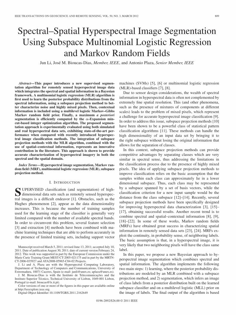
Fig. 1. Illustration of the advantages that can be gained by usingsubspace projection under the linear mixture model assumption, where{m(1),m(2),m(3)} denote the spectral endmembers, to reduce the impactof mixed pixels in the classification process.

a certain class is very small, our proposed approach can stillprovide good performance in such ill-posed problems, providedthat the method is able to obtain a good estimate of the subspacein which the considered class lives. Fig. 1 shows the advantagesthat can be gained by using subspace projection under the linearmixture model assumption. As shown by Fig. 1, hyperspectraldata generally live in class-independent subspaces given by thespectral endmembers. Subsequently, the projection into suchsubspaces allows us to specifically avoid spectral confusion dueto mixed pixels, thus reducing their impact in the subsequentclassification process.

With this in mind, we may then write the observation mech-anism for class k as

x(k)i = U(k)z

(k)i + n

(k)i (5)

where n(k)i is the noise of class k, U(k) = {u(k)

1 , . . . ,u(k)

r(k)}is a set of r(k)-dimensional orthonormal basis vectors forthe subspace associated with class k, and z

(k)i is, apart from

the noise n(k)i , the coordinates of x

(k)i with respect to the

basis U(k).We assume that the class-independent random vectors n

(k)i

and z(k)i are Gaussian distributed with zero mean and diago-

nal covariance matrices, i.e., n(k)i ∼ N (0, σ(k)2I) and z

(k)i ∼

N (0, α(k)I). We are aware that, statistically, these assumptionsare very strong and that they rarely hold in real data. However,they allow us to preserve the subspace-based structure of ourmodel and yield a robust discriminative model. Hence, we havedecided to preserve these assumptions in our implementation.In addition to this, we also emphasize that, accordingly, nor-malization of the input data is not needed in order for the pro-posed model to perform properly. Based on the aforementionedassumptions, we have the following generative model:

p(xi|yi = k) ∼ N(0, α(k)U(k)U(k)T + σ(k)2I

). (6)


Under the present setup, the generative model in (6) can becomputed as follows:

p(xi|yi = k)

∝exp

{−1

2xTi

(α(k)U(k)U(k)T+σ(k)2I

)−1

xi

}=exp

{−1

2xTi

(I

σ(k)2−U(k)

σ(k)2

×(

I

α(k)+U(k)TU(k)

σ(k)2

)−1U(k)T

σ(k)2

⎞⎠xi

⎫⎬⎭=exp

{− 1

2σ(k)2xTi

(1− α(k)

α(k)+σ(k)2U(k)U(k)T

)xi

}=exp

{−1

2

xTi x

σ(k)2+

1

2σ(k)2

α(k)

α(k)+σ(k)2

∥∥∥xTi U

(k)∥∥∥2} . (7)

Let ω(k)1 ≡ −(1/2σ(k)2), ω

(k)2 ≡ (1/2σ(k)2)(α(k)/(α(k) +

σ(k)2)), ω(k) ≡ [ω(k)1 ω

(k)2 ]T, and ω ≡ [ω(1)T , . . . ,ω(K)T ]T.

With these definitions in mind, we can compute the posteriorclass density p(yi|xi) as follows:

p(yi=k|xi,ω)=p(xi|yi=k,ω)p(yi=k)∑Kk=1 p(xi|yi=k,ω)p(yi=k)

=exp

(ω(k)Tφ(k)(xi)

)p(yi=k)∑K

k=1 exp(ω(k)Tφ(k)(xi)

)p(yi=k)

(8)

where φ(k)(xi) = [‖xi‖2, ‖xTi U

(k)‖2]T. Assuming equiprob-able classes, i.e., p(yi = k) = 1/K, the problem in (8) turns to

p(yi = k|xi,ω) =exp

(ω(k)φ(k)(xi)

)∑K

k=1 exp(ω(k)φ(k)(xi)

) (9)

which is exactly an MLR [7].1) Learning the Class-Independent Subspace: Let R(k) =

〈x(k)

l(k)x(k)T

l(k) 〉 denote the sample correlation matrix associatedwith class k determined from the training set. By computingthe eigendecomposition of R(k), we have

R(k) = E(k)Λ(k)E(k)T (10)

where E(k) = {e(k)1 , . . . , e(k)d } is the eigenvector matrix and

Λ = diag(λ(k)1 , . . . , λ

(k)d ) is the eigenvalue matrix with de-

creasing magnitude, i.e., λ(k)1 ≥ · · · ≥ λ

(k)d . Moreover, for i ∈

S , vector xi can be represented as a sum of two mutuallyorthogonal vectors xi = xi + xi, where xi is the projection ofvector xi on the r(k)-dimensional subspace spanned by the firstr(k) eigenvalues, i.e., λ(k)

1 , . . . , λ(k)

r(k) , and xi is the projection onthe orthogonal subspace spanned by the remaining eigenvalues.

We take U(k) = {e(k)1 , . . . , e(k)

r(k)} as an estimate of the class-independent r(k)-dimensional subspace with r(k) < d and

r(k) = min

⎧⎨⎩r(k) :

r(k)∑i=1

λ(k)i ≥

d∑i=1

λ(k)i × τ

⎫⎬⎭ (11)

where 0 ≤ τ ≤ 1 is a threshold parameter controlling theloss of spectral information after projecting the data into thesubspace.

2) Learning the MLR Regressors: In order to cope withdifficulties in learning the regression vector ω associated withbad or ill conditioning of the underlying inverse problem, weadopt a quadratic prior on ω so that

p(ω) ∝ e−β/2‖ω‖2 (12)

where β ≥ 0 is a regularization parameter controlling weight ofthe prior.

In the present problem, learning the class densities amountsto estimating the logistic regressors ω. Inspired by previousworks [7], [8], [18], [22], [30], we compute ω by calculatingthe MAP estimate

ω = argmaxω

(ω) + log p(ω) (13)

where (ω) is the log-likelihood function given by

(ω) ≡ logl∏

i=1

p(yi|xi,ω). (14)

The optimization problem in (13) is concave, although theterm (ω) is nonquadratic. This term can be approximated bya quadratic lower bound given by [7]; for any k ∈ K and theregressors ωt at iteration t, we have

(ω(k)

)≥

(ω

(k)t

)+(ω(k) − ω

(k)t

)T

g(ω

(k)t

)+1

2

(ω(k) − ω

(k)t

)T

B(k)(ω(k) − ω

(k)t

)(15)

with

B(k) ≡ −(1/2)[I− 11T/(K + 1)

]⊗

l∑i=1

φ(k)(xi)φ(k)(xi)

T

(16)

where 1 denotes a column vector of ones and g(ω(k)t ) is

the gradient of (·) at ω(k)t . Based on the lower bound (15),

we implement an instance of the minorization–maximization(MM) algorithm [31], which consists in replacing, in eachiteration, the objective function (ω) with the lower bound (15)and then in maximizing it. It should be noted that the well-known expectation–maximization (EM) algorithm [32] is, infact, an MM algorithm and that not all MM algorithms are EMinstances. The aforementioned procedure then leads to

ω(k)t+1 = argmax

ω(k)ω(k)T

(g(ω

(k)t

)−B(k)ω

(k)t

)+1

2ω(k)T

(B(k) − βI

)ω(k). (17)


Now, the optimization problem in (17) is quadratic and easy tosolve, leading to the following update function:

ω(k)t+1=

1

2

(B(k) − βI

)−1(B(k)ω

(k)t − g

(ω

(k)t

)),

for k ∈ K. (18)

We note that matrix (B(k) − βI)−1 is negative definite and,thus, nonsingular. Furthermore, it is fixed along the algorithmiterations; thus, it can be precomputed. With this in mind, itis now possible to perform an exact MAP-based MLR undera quadratic prior. The pseudocode for the subspace projection-based MLR algorithm, referred to hereinafter as MLRsub, isshown in Algorithm 1. In the algorithm description, itersdenotes the maximum number of iterations. The overall com-plexity of Algorithm 1 is dominated by the computation of thecorrelation matrix, which has complexity O(ld2) (recall that lis the number of labeled samples and d is the dimensionality ofthe feature vectors).

Algorithm 1 MLRsub

Input: ω0, Dl, β, τ , itersOutput: ω, U ≡ {U(1), . . . ,U(k)}for k = 1 to K do

U(k) ≡ U(X (k)

l(k) , τ) (∗ U computes the subspace ac-cording to (10)∗)

B(k) ≡ B(U(k),Dl) (∗ B computes the systemmatrix B according to (16)∗)

end fort := 1while t ≤ iters or stopping criterion is not satisfied do

for k := 1 to K dog(ω

(k)t−1) ≡ ∇(ω

(k)t−1)

ω(k)t = solution{B(k),g(ω

(k)t−1),U

(k), β}end for

end while

B. MRF-Based MLL Spatial Prior

In order to improve the classification performance achievedby using the spectral information alone, in this paper, weintegrate the contextual information with spectral informationby using an isotropic MLL prior to modeling the image of classlabels y. This approach exploits the fact that, in segmentingreal-world images, it is very likely that spatially neighboringpixels belong to the same class. This prior, which belongs to theMRF class, encourages piecewise smooth segmentations andpromotes solutions in which adjacent pixels are likely to belongto the same class. The MLL prior constitutes a generalizationof the Ising model [33] and has been widely used in imagesegmentation problems [34].

According to the Hammersly–Clifford theorem [35], thedensity associated with an MRF is a Gibbs’ distribution [33].

Therefore, the prior model for segmentation has the followingstructure:

p(y) =1

Ze

(−∑c∈C

Vc(y)

)(19)

where Z is a normalizing constant for the density, the sum inthe exponent is over the so-called prior potentials Vc(y) for theset of cliques2 C over the image, and

−Vc(y) =

⎧⎨⎩υyi

, if |c| = 1 (single clique)μc, if |c| > 1 and ∀i,j∈cyi = yj−μc, if |c| > 1 and ∃i,j∈cyi �= yj

(20)

where μc is a nonnegative constant. The potential function in(20) encourages neighbors to have the same label. The intro-duced MLL prior offers a great deal of flexibility by allowingvariations of the set of cliques and the parameters υyi

and μc.For example, the model generates texturelike regions if μc

depends on c and bloblike regions otherwise [34]. In this paper,we take υyi

= cte and μc = (1/2)μ > 0. Thus, (19) can berewritten as follows:

p(y) =1

Ze

μ∑

(i,j)∈C

δ(yi−yj)

(21)

where δ(y) is the unit impulse function.3 This choice givesno preference to any direction concerning. A straightforwardcomputation of p(yi), i.e., the marginal of p(y) with respect toyi, leads to p(yi) being constant and, thus, equiprobable, whichis therefore compatible with the assumption made in (2) and (8).Notice that the pairwise interaction terms δ(yi − yj) attachhigher probability to equal neighboring labels than the otherway around. In this way, the MLL prior promotes piecewisesmooth segmentations, where parameter μ controls the level ofsmoothness.

C. MAP Estimate via Graph Cuts

Let us assume that the posterior class densities p(yi|xi)are estimated using (8). Let us also assume that the MLLprior p(y) is estimated using (21). According to (3), the MAPsegmentation is finally given by

y = arg miny∈Kn

⎧⎨⎩∑i∈S

− log p(yi|xi, ω)− μ∑i∼j

δ(yi − yj)

⎫⎬⎭ .

(22)

This is a combinatorial optimization problem involving unaryand pairwise interaction terms, which is very difficult to com-pute. Several new algorithms such as graph cuts [25], [36],[37], loopy belief propagation [38], [39], and tree-reweightedmessage passing [40] have been proposed in the literature inorder to tackle this optimization problem. In this paper, weresort to the α-Expansion graph-cut-based algorithm [25], [41].

2A clique is a single term or either a set of pixels that are neighbors of oneanother.

3That is, δ(0) = 1 and δ(y) = 0 for y �= 0.


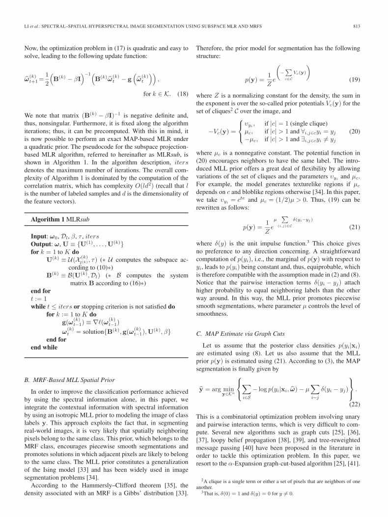
Fig. 2. Block diagram summarizing the most relevant steps of the proposed MLRsubMLL algorithm.

This method yields good approximations to the MAP segmenta-tion and is quite efficient from a computational viewpoint, withpractical computational complexity O(n) [25].

D. Supervised Segmentation Algorithm: MLRsubMLL

To conclude the description of our proposed method,Algorithm 2 provides a pseudocode for our newly developedsupervised segmentation algorithm based on a subspace MLRclassifier with MRF-based MLL prior. This algorithm, calledMLRsubMLL hereinafter, integrates all the different modulesdescribed in this section. Specifically, line 3 in Algorithm 2learns the logistic regressors using MLRsub, which is applied tothe full hyperspectral image. Here, the quadratic regularizationparameter β ≥ 0 is used to tackle ill-conditioned problems.Line 4 in Algorithm 2 computes the probabilities based onthe outcome of MLRsub. Line 5 in Algorithm 2 efficientlycomputes the MAP segmentation by applying the α-Expansiongraph-cut-based algorithm, where the neighborhood pa-rameter μ determines the strength of the spatial prior. Forillustrative purposes, Fig. 2 summarizes the most relevant stepsof the newly proposed segmentation algorithm using a blockdiagram.

Algorithm 2 MLRsubMLL

1: Input: x, Dl, β, τ , μ2: Output: y3: {ω,U} = MLRsub{Dl, β, τ}4: P := p(x, ω,U) (∗ P collects the probabilities in (9)∗)5: y := α− Expansion(P, μ, neighborhood)

The overall complexity of the proposed MLRsubMLL al-gorithm is dominated by the MLRsub algorithm inferring theregressors, which has computational complexity O(ld2), andalso by the α-Expansion algorithm used to determine the MAPsegmentation, which has practical complexity O(n). In conclu-sion, if ld2 > n (e.g., the problem is high dimensional, with alarge number of training samples), then the overall complexityis dominated by the subspace-based learning step. Otherwise, ifld2 < n (e.g., the problem is given by a large number of pixels),then the overall complexity is dominated by the α-Expansionalgorithm.

IV. EXPERIMENTAL RESULTS

This section uses both simulated and real hyperspectral datasets to illustrate the effectiveness of the proposed MLRsubMLL

segmentation algorithm in different analysis scenarios. Themain goal of using simulated data sets is to assess the per-formance of the algorithm in a fully controlled environment,whereas the main goal of using real data sets is to comparethe algorithm with other state-of-the-art analysis techniquesusing widely used hyperspectral scenes. The remainder of thissection is organized as follows. Section IV-A first explainsthe parameter settings adopted in our experimental evaluation.Section IV-B then evaluates the proposed MLRsubMLL al-gorithm by using simulated data sets, whereas Section IV-Cevaluates the proposed segmentation algorithm using real hy-perspectral images.

A. Parameter Settings

Before describing our results with simulated and real hyper-spectral data sets, it is first important to discuss the parametersettings adopted in our experiments. In our tests, we assumel(k) � l/K for k ∈ K. For small classes, if the total number oflabeled samples per class k in the ground-truth image, for ex-ample, L(k), is smaller than l/K, we take l(k) = L(k)/2. In thiscase, we use more labeled samples to represent large classes. Itshould be noted that, in all experiments, the labeled sets Dl arerandomly selected from the available labeled samples and thatthe remaining samples are used for validation. Each value ofoverall accuracy [OA (in percent)] is obtained after conductingten Monte Carlo runs with respect to the labeled samplesDl. The labeled samples for each Monte Carlo simulation areobtained by resampling the available labeled samples. Prior tothe experiments, we infer the setting of the quadratic parameterβ. In practice, β is relevant to the condition number of B(k) fork ∈ K. In this paper, we set β = e−10 for all experiments.

B. Experiments With Simulated Hyperspectral Data

In our experiments, we have generated a simulated hy-perspectral scene as follows. First, we generate an image offeatures using a linear mixture model

xi =K∑

k=1

m(k)γ(k)i + ni (23)

with K = 10. Here, m(k) for k ∈ K are spectral signatures ob-tained from the U.S. Geological Survey (USGS) digital spectrallibrary,4 and xi is a simulated mixed pixel. An MLL distributionwith smoothness parameter μ = 2 is used to generate the spatialinformation, and the total size of the simulated image is of

4The USGS library of spectral signatures is available online: http://speclab.cr.usgs.gov.


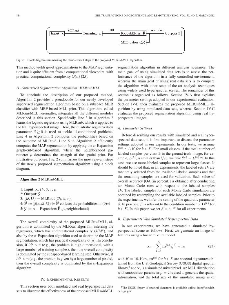
Fig. 3. Classification and segmentation maps obtained after applying the proposed method to a simulated hyperspectral scene with σ = 0.8 and γ = 0.7 byusing τ = 0.9, l = 288, and μ = 2. (a) Ground-truth class labels. (b) Classification result (OA = 49.09%). (c) Segmentation result (OA = 94.34%).

120 × 120 pixels. Zero-mean Gaussian noise with covarianceσ2I, i.e., ni ∼ N (0, σ2I) is finally added to our simple simu-lated hyperspectral scene. For illustrative purposes, the imageof class labels y is shown in Fig. 3(a). Assume that xi hasclass label yi = kk; then, we define γ

(kk)i as the abundance

of the objective class and γ(k)i (for k ∈ K and k �= kk) as the

abundance of the remaining signatures which contribute to themixed pixel, where γ

(k)i values are generated according to a

simple uniform distribution in the proposed problem. In orderto simplify notations, we take γ

(kk)i = γ,

∑k∈K,k �=ki

γ(k)i =

1− γ, and we use the same γ for all pixels.We have conducted five different experiments with the sim-

ulated hyperspectral image described earlier. These experi-ments have been carefully designed in order to analyze severalrelevant aspects of our proposed MLRsubMLL segmentationalgorithm in a fully controlled environment.

1) In our first experiment, we evaluate the impact of thepresence of mixed pixels on the segmentation output.

2) In our second experiment, we analyze the impact of theparameter τ (controlling the amount of spectral informa-tion retained after subspace projection) on the segmenta-tion output.

3) In our third experiment, we evaluate the impact of thetraining set size on the segmentation output.

4) In our fourth experiment, we analyze the impact of thesmoothness parameter μ on the segmentation output.

5) In our fifth experiment, we evaluate the impact of noiseon the segmentation output.

In all these experiments, we will use the optimal value ofclassification accuracy (OAopt) as a reference to evaluate thegoodness of our reported OA scores. Here, OAopt ≡ 100(1−Pe)%, where Pe is defined as follows [42]:

Pe = p(yi �= yi) (24)

where yi and yi are the true label and the MAP estimate,respectively, i.e.,

yi = argmaxyi

p(yi|xi).

For a multiclass problem, we use the following error bound asan alternative since (24) is difficult to compute:

erfc

(distmin

2σ

)≤ Pe ≤

K − 1

2erfc

(distmin

2σ

)(25)

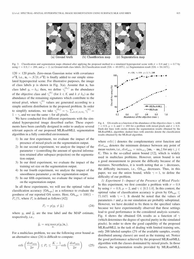
Fig. 4. OA results as a function of the abundance of the objective class: γ, withτ = 0.9, μ = 2, and l = 288 for a problem with mixed pixels and σ = 0.8.Dash–dot lines with circles denote the segmentation results obtained by theMLRsubMLL algorithm; dashed lines with asterisks denote the classificationresults obtained by the MLRsub algorithm.

where erfc(·) denotes the complementary error function anddistmin denotes the minimum distance between any point ofmean vectors, i.e., distmin = mini�=j ‖mi −mj‖ for any i, j ∈K. This is the so-called union bound [12], which is widelyused in multiclass problems. However, union bound is nota good measurement to present the difficulty because of themixtures. Nevertheless, it is worth noting that as γ decreases,the difficulty increases, i.e., OAopt decreases. Thus, in thispaper, we use the union bound, while γ = 1, to define thedifficulty of our problem.

1) Experiment 1—Impact of the Presence of Mixed Pixels:In this experiment, we first consider a problem with σ = 0.8by using τ = 0.9, μ = 2, and γ ∈ [0.5 1.0]. In this context, theoptimal value of classification accuracy is given by OAopt ≤71.04% with γ = 1. It should be noted that the values ofparameters τ and μ in our simulation are probably suboptimal.However, we have decided to fix them to the specified valuesbecause we have experimentally observed that these settingslead to good performance in the considered analysis scenario.Fig. 4 shows the obtained OA results as a function of γ(which determines the degree of spectral purity in the simulatedpixels). In order to show the good capability of the proposedMLRsubMLL in the task of dealing with limited training sets,only 288 labeled samples (2% of the available samples, evenlydistributed among classes) are used as the training set. Noticethe good performance achieved by the proposed MLRsubMLLalgorithm with the classes dominated by mixed pixels. In thoseclasses, the segmentation results provided by MLRsubMLL


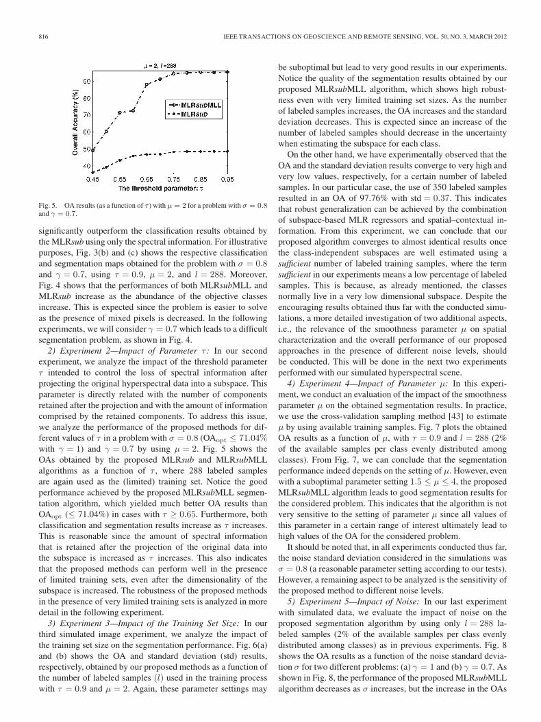
Fig. 5. OA results (as a function of τ ) with μ = 2 for a problem with σ = 0.8and γ = 0.7.

significantly outperform the classification results obtained bythe MLRsub using only the spectral information. For illustrativepurposes, Fig. 3(b) and (c) shows the respective classificationand segmentation maps obtained for the problem with σ = 0.8and γ = 0.7, using τ = 0.9, μ = 2, and l = 288. Moreover,Fig. 4 shows that the performances of both MLRsubMLL andMLRsub increase as the abundance of the objective classesincrease. This is expected since the problem is easier to solveas the presence of mixed pixels is decreased. In the followingexperiments, we will consider γ = 0.7 which leads to a difficultsegmentation problem, as shown in Fig. 4.

2) Experiment 2—Impact of Parameter τ : In our secondexperiment, we analyze the impact of the threshold parameterτ intended to control the loss of spectral information afterprojecting the original hyperspectral data into a subspace. Thisparameter is directly related with the number of componentsretained after the projection and with the amount of informationcomprised by the retained components. To address this issue,we analyze the performance of the proposed methods for dif-ferent values of τ in a problem with σ = 0.8 (OAopt ≤ 71.04%with γ = 1) and γ = 0.7 by using μ = 2. Fig. 5 shows theOAs obtained by the proposed MLRsub and MLRsubMLLalgorithms as a function of τ , where 288 labeled samplesare again used as the (limited) training set. Notice the goodperformance achieved by the proposed MLRsubMLL segmen-tation algorithm, which yielded much better OA results thanOAopt (≤ 71.04%) in cases with τ ≥ 0.65. Furthermore, bothclassification and segmentation results increase as τ increases.This is reasonable since the amount of spectral informationthat is retained after the projection of the original data intothe subspace is increased as τ increases. This also indicatesthat the proposed methods can perform well in the presenceof limited training sets, even after the dimensionality of thesubspace is increased. The robustness of the proposed methodsin the presence of very limited training sets is analyzed in moredetail in the following experiment.

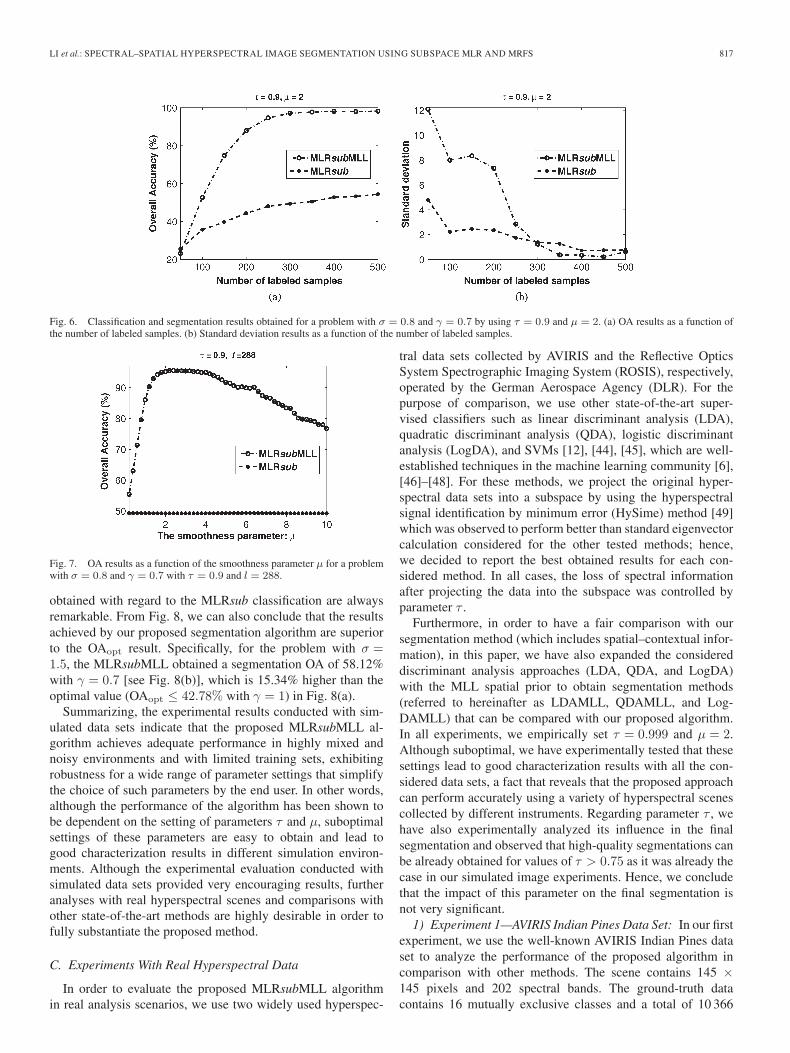
3) Experiment 3—Impact of the Training Set Size: In ourthird simulated image experiment, we analyze the impact ofthe training set size on the segmentation performance. Fig. 6(a)and (b) shows the OA and standard deviation (std) results,respectively, obtained by our proposed methods as a function ofthe number of labeled samples (l) used in the training processwith τ = 0.9 and μ = 2. Again, these parameter settings may

be suboptimal but lead to very good results in our experiments.Notice the quality of the segmentation results obtained by ourproposed MLRsubMLL algorithm, which shows high robust-ness even with very limited training set sizes. As the numberof labeled samples increases, the OA increases and the standarddeviation decreases. This is expected since an increase of thenumber of labeled samples should decrease in the uncertaintywhen estimating the subspace for each class.

On the other hand, we have experimentally observed that theOA and the standard deviation results converge to very high andvery low values, respectively, for a certain number of labeledsamples. In our particular case, the use of 350 labeled samplesresulted in an OA of 97.76% with std = 0.37. This indicatesthat robust generalization can be achieved by the combinationof subspace-based MLR regressors and spatial–contextual in-formation. From this experiment, we can conclude that ourproposed algorithm converges to almost identical results oncethe class-independent subspaces are well estimated using asufficient number of labeled training samples, where the termsufficient in our experiments means a low percentage of labeledsamples. This is because, as already mentioned, the classesnormally live in a very low dimensional subspace. Despite theencouraging results obtained thus far with the conducted simu-lations, a more detailed investigation of two additional aspects,i.e., the relevance of the smoothness parameter μ on spatialcharacterization and the overall performance of our proposedapproaches in the presence of different noise levels, shouldbe conducted. This will be done in the next two experimentsperformed with our simulated hyperspectral scene.

4) Experiment 4—Impact of Parameter μ: In this experi-ment, we conduct an evaluation of the impact of the smoothnessparameter μ on the obtained segmentation results. In practice,we use the cross-validation sampling method [43] to estimateμ by using available training samples. Fig. 7 plots the obtainedOA results as a function of μ, with τ = 0.9 and l = 288 (2%of the available samples per class evenly distributed amongclasses). From Fig. 7, we can conclude that the segmentationperformance indeed depends on the setting of μ. However, evenwith a suboptimal parameter setting 1.5 ≤ μ ≤ 4, the proposedMLRsubMLL algorithm leads to good segmentation results forthe considered problem. This indicates that the algorithm is notvery sensitive to the setting of parameter μ since all values ofthis parameter in a certain range of interest ultimately lead tohigh values of the OA for the considered problem.

It should be noted that, in all experiments conducted thus far,the noise standard deviation considered in the simulations wasσ = 0.8 (a reasonable parameter setting according to our tests).However, a remaining aspect to be analyzed is the sensitivity ofthe proposed method to different noise levels.

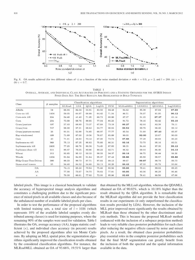
5) Experiment 5—Impact of Noise: In our last experimentwith simulated data, we evaluate the impact of noise on theproposed segmentation algorithm by using only l = 288 la-beled samples (2% of the available samples per class evenlydistributed among classes) as in previous experiments. Fig. 8shows the OA results as a function of the noise standard devia-tion σ for two different problems: (a) γ = 1 and (b) γ = 0.7. Asshown in Fig. 8, the performance of the proposed MLRsubMLLalgorithm decreases as σ increases, but the increase in the OAs


Fig. 6. Classification and segmentation results obtained for a problem with σ = 0.8 and γ = 0.7 by using τ = 0.9 and μ = 2. (a) OA results as a function ofthe number of labeled samples. (b) Standard deviation results as a function of the number of labeled samples.

Fig. 7. OA results as a function of the smoothness parameter μ for a problemwith σ = 0.8 and γ = 0.7 with τ = 0.9 and l = 288.

obtained with regard to the MLRsub classification are alwaysremarkable. From Fig. 8, we can also conclude that the resultsachieved by our proposed segmentation algorithm are superiorto the OAopt result. Specifically, for the problem with σ =1.5, the MLRsubMLL obtained a segmentation OA of 58.12%with γ = 0.7 [see Fig. 8(b)], which is 15.34% higher than theoptimal value (OAopt ≤ 42.78% with γ = 1) in Fig. 8(a).

Summarizing, the experimental results conducted with sim-ulated data sets indicate that the proposed MLRsubMLL al-gorithm achieves adequate performance in highly mixed andnoisy environments and with limited training sets, exhibitingrobustness for a wide range of parameter settings that simplifythe choice of such parameters by the end user. In other words,although the performance of the algorithm has been shown tobe dependent on the setting of parameters τ and μ, suboptimalsettings of these parameters are easy to obtain and lead togood characterization results in different simulation environ-ments. Although the experimental evaluation conducted withsimulated data sets provided very encouraging results, furtheranalyses with real hyperspectral scenes and comparisons withother state-of-the-art methods are highly desirable in order tofully substantiate the proposed method.

C. Experiments With Real Hyperspectral Data

In order to evaluate the proposed MLRsubMLL algorithmin real analysis scenarios, we use two widely used hyperspec-

tral data sets collected by AVIRIS and the Reflective OpticsSystem Spectrographic Imaging System (ROSIS), respectively,operated by the German Aerospace Agency (DLR). For thepurpose of comparison, we use other state-of-the-art super-vised classifiers such as linear discriminant analysis (LDA),quadratic discriminant analysis (QDA), logistic discriminantanalysis (LogDA), and SVMs [12], [44], [45], which are well-established techniques in the machine learning community [6],[46]–[48]. For these methods, we project the original hyper-spectral data sets into a subspace by using the hyperspectralsignal identification by minimum error (HySime) method [49]which was observed to perform better than standard eigenvectorcalculation considered for the other tested methods; hence,we decided to report the best obtained results for each con-sidered method. In all cases, the loss of spectral informationafter projecting the data into the subspace was controlled byparameter τ .

Furthermore, in order to have a fair comparison with oursegmentation method (which includes spatial–contextual infor-mation), in this paper, we have also expanded the considereddiscriminant analysis approaches (LDA, QDA, and LogDA)with the MLL spatial prior to obtain segmentation methods(referred to hereinafter as LDAMLL, QDAMLL, and Log-DAMLL) that can be compared with our proposed algorithm.In all experiments, we empirically set τ = 0.999 and μ = 2.Although suboptimal, we have experimentally tested that thesesettings lead to good characterization results with all the con-sidered data sets, a fact that reveals that the proposed approachcan perform accurately using a variety of hyperspectral scenescollected by different instruments. Regarding parameter τ , wehave also experimentally analyzed its influence in the finalsegmentation and observed that high-quality segmentations canbe already obtained for values of τ > 0.75 as it was already thecase in our simulated image experiments. Hence, we concludethat the impact of this parameter on the final segmentation isnot very significant.

1) Experiment 1—AVIRIS Indian Pines Data Set: In our firstexperiment, we use the well-known AVIRIS Indian Pines dataset to analyze the performance of the proposed algorithm incomparison with other methods. The scene contains 145 ×145 pixels and 202 spectral bands. The ground-truth datacontains 16 mutually exclusive classes and a total of 10 366


Fig. 8. OA results achieved (for two different values of γ) as a function of the noise standard deviation σ with τ = 0.9, μ = 2, and l = 288. (a) γ = 1.(b) γ = 0.7.

TABLE IOVERALL, AVERAGE, AND INDIVIDUAL CLASS ACCURACIES (IN PERCENT) AND κ STATISTIC OBTAINED FOR THE AVIRIS INDIAN

PINES DATA SET. THE BEST RESULTS ARE HIGHLIGHTED IN BOLD TYPEFACE

labeled pixels. This image is a classical benchmark to validatethe accuracy of hyperspectral image analysis algorithms andconstitutes a challenging problem due to the significant pres-ence of mixed pixels in all available classes and also because ofthe unbalanced number of available labeled pixels per class.

In order to test the performance of the proposed algorithmswith limited training sets, a total size of l = 1036 (whichrepresents 10% of the available labeled samples evenly dis-tributed among classes) is used for training purposes, where theremaining 90% of the samples were used for validation. Table Iillustrates the OA, average accuracy (AA), kappa statistic coef-ficient (κ), and individual class accuracy (in percent) resultsachieved by the proposed algorithms after ten Monte Carloruns. By adopting an MLL spatial prior, the segmentation algo-rithms significantly improved the classification results obtainedby the considered classification algorithms. For instance, theMLRsubMLL obtained an OA of 93.66%, 19.51% larger than

that obtained by the MLLsub algorithm, whereas the QDAMLLobtained an OA of 90.02%, which is 10.18% higher than theresult obtained by the QDA algorithm. It is remarkable thatthe MLRsub algorithm did not provide the best classificationresults in our experiments (it only outperformed the classifica-tion results provided by LDA). However, the inclusion of theMLL prior improved more significantly the results obtained byMLRsub than those obtained by the other discriminant anal-ysis methods. This is because the proposed MLRsub method(enhanced with the inclusion of a subspace projection method)leads to very reliable class posterior probabilities for each classafter reducing the negative effects caused by noise and mixedpixels. As a result, the obtained class posterior probabilitiesplay essential roles in the complete posterior probabilities suchthat the final MAP segmentation can greatly benefit fromthe inclusion of both the spectral and the spatial informationavailable in the data.


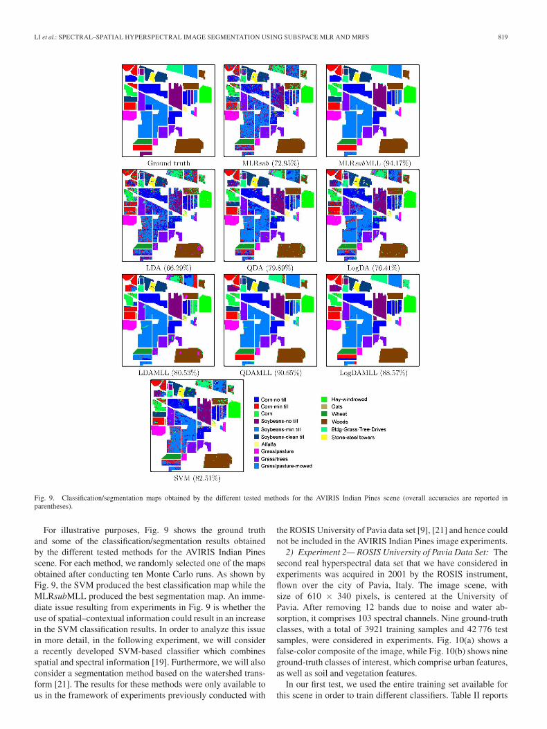
Fig. 9. Classification/segmentation maps obtained by the different tested methods for the AVIRIS Indian Pines scene (overall accuracies are reported inparentheses).

For illustrative purposes, Fig. 9 shows the ground truthand some of the classification/segmentation results obtainedby the different tested methods for the AVIRIS Indian Pinesscene. For each method, we randomly selected one of the mapsobtained after conducting ten Monte Carlo runs. As shown byFig. 9, the SVM produced the best classification map while theMLRsubMLL produced the best segmentation map. An imme-diate issue resulting from experiments in Fig. 9 is whether theuse of spatial–contextual information could result in an increasein the SVM classification results. In order to analyze this issuein more detail, in the following experiment, we will considera recently developed SVM-based classifier which combinesspatial and spectral information [19]. Furthermore, we will alsoconsider a segmentation method based on the watershed trans-form [21]. The results for these methods were only available tous in the framework of experiments previously conducted with

the ROSIS University of Pavia data set [9], [21] and hence couldnot be included in the AVIRIS Indian Pines image experiments.

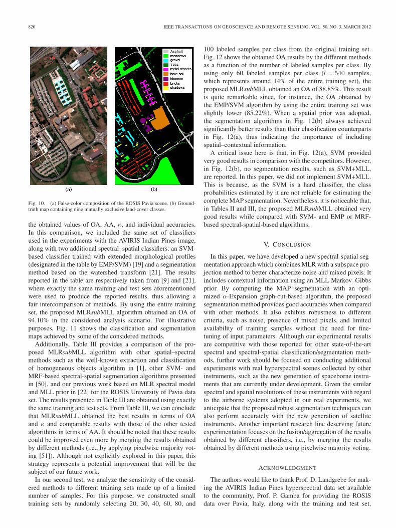
2) Experiment 2— ROSIS University of Pavia Data Set: Thesecond real hyperspectral data set that we have considered inexperiments was acquired in 2001 by the ROSIS instrument,flown over the city of Pavia, Italy. The image scene, withsize of 610 × 340 pixels, is centered at the University ofPavia. After removing 12 bands due to noise and water ab-sorption, it comprises 103 spectral channels. Nine ground-truthclasses, with a total of 3921 training samples and 42 776 testsamples, were considered in experiments. Fig. 10(a) shows afalse-color composite of the image, while Fig. 10(b) shows nineground-truth classes of interest, which comprise urban features,as well as soil and vegetation features.

In our first test, we used the entire training set available forthis scene in order to train different classifiers. Table II reports


Fig. 10. (a) False-color composition of the ROSIS Pavia scene. (b) Ground-truth map containing nine mutually exclusive land-cover classes.

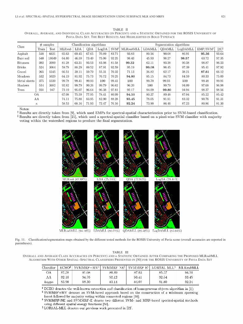
the obtained values of OA, AA, κ, and individual accuracies.In this comparison, we included the same set of classifiersused in the experiments with the AVIRIS Indian Pines image,along with two additional spectral–spatial classifiers: an SVM-based classifier trained with extended morphological profiles(designated in the table by EMP/SVM) [19] and a segmentationmethod based on the watershed transform [21]. The resultsreported in the table are respectively taken from [9] and [21],where exactly the same training and test sets aforementionedwere used to produce the reported results, thus allowing afair intercomparison of methods. By using the entire trainingset, the proposed MLRsubMLL algorithm obtained an OA of94.10% in the considered analysis scenario. For illustrativepurposes, Fig. 11 shows the classification and segmentationmaps achieved by some of the considered methods.

Additionally, Table III provides a comparison of the pro-posed MLRsubMLL algorithm with other spatial–spectralmethods such as the well-known extraction and classificationof homogeneous objects algorithm in [1], other SVM- andMRF-based spectral-spatial segmentation algorithms presentedin [50], and our previous work based on MLR spectral modeland MLL prior in [22] for the ROSIS University of Pavia dataset. The results presented in Table III are obtained using exactlythe same training and test sets. From Table III, we can concludethat MLRsubMLL obtained the best results in terms of OAand κ and comparable results with those of the other testedalgorithms in terms of AA. It should be noted that these resultscould be improved even more by merging the results obtainedby different methods (i.e., by applying pixelwise majority vot-ing [51]). Although not explicitly explored in this paper, thisstrategy represents a potential improvement that will be thesubject of our future work.

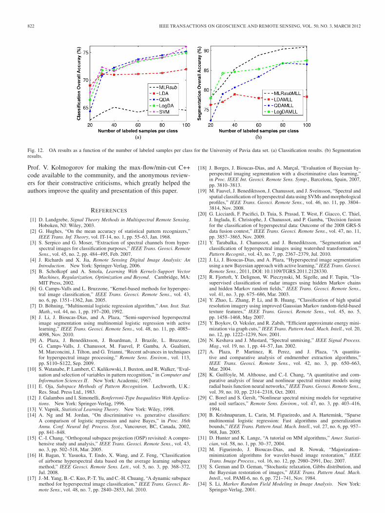
In our second test, we analyze the sensitivity of the consid-ered methods to different training sets made up of a limitednumber of samples. For this purpose, we constructed smalltraining sets by randomly selecting 20, 30, 40, 60, 80, and

100 labeled samples per class from the original training set.Fig. 12 shows the obtained OA results by the different methodsas a function of the number of labeled samples per class. Byusing only 60 labeled samples per class (l = 540 samples,which represents around 14% of the entire training set), theproposed MLRsubMLL obtained an OA of 88.85%. This resultis quite remarkable since, for instance, the OA obtained bythe EMP/SVM algorithm by using the entire training set wasslightly lower (85.22%). When a spatial prior was adopted,the segmentation algorithms in Fig. 12(b) always achievedsignificantly better results than their classification counterpartsin Fig. 12(a), thus indicating the importance of includingspatial–contextual information.

A critical issue here is that, in Fig. 12(a), SVM providedvery good results in comparison with the competitors. However,in Fig. 12(b), no segmentation results, such as SVM+MLL,are reported. In this paper, we did not implement SVM+MLL.This is because, as the SVM is a hard classifier, the classprobabilities estimated by it are not reliable for estimating thecomplete MAP segmentation. Nevertheless, it is noticeable that,in Tables II and III, the proposed MLRsubMLL obtained verygood results while compared with SVM- and EMP or MRF-based spectral-spatial-based algorithms.

V. CONCLUSION

In this paper, we have developed a new spectral-spatial seg-mentation approach which combines MLR with a subspace pro-jection method to better characterize noise and mixed pixels. Itincludes contextual information using an MLL Markov–Gibbsprior. By computing the MAP segmentation with an opti-mized α-Expansion graph-cut-based algorithm, the proposedsegmentation method provides good accuracies when comparedwith other methods. It also exhibits robustness to differentcriteria, such as noise, presence of mixed pixels, and limitedavailability of training samples without the need for fine-tuning of input parameters. Although our experimental resultsare competitive with those reported for other state-of-the-artspectral and spectral-spatial classification/segmentation meth-ods, further work should be focused on conducting additionalexperiments with real hyperspectral scenes collected by otherinstruments, such as the new generation of spaceborne instru-ments that are currently under development. Given the similarspectral and spatial resolutions of these instruments with regardto the airborne systems adopted in our real experiments, weanticipate that the proposed robust segmentation techniques canalso perform accurately with the new generation of satelliteinstruments. Another important research line deserving futureexperimentation focuses on the fusion/aggregation of the resultsobtained by different classifiers, i.e., by merging the resultsobtained by different methods using pixelwise majority voting.

ACKNOWLEDGMENT

The authors would like to thank Prof. D. Landgrebe for mak-ing the AVIRIS Indian Pines hyperspectral data set availableto the community, Prof. P. Gamba for providing the ROSISdata over Pavia, Italy, along with the training and test set,


TABLE IIOVERALL, AVERAGE, AND INDIVIDUAL CLASS ACCURACIES (IN PERCENT) AND κ STATISTIC OBTAINED FOR THE ROSIS UNIVERSITY OF

PAVIA DATA SET. THE BEST RESULTS ARE HIGHLIGHTED IN BOLD TYPEFACE

Fig. 11. Classification/segmentation maps obtained by the different tested methods for the ROSIS University of Pavia scene (overall accuracies are reported inparentheses).

TABLE IIIOVERALL AND AVERAGE CLASS ACCURACIES (IN PERCENT) AND κ STATISTIC OBTAINED AFTER COMPARING THE PROPOSED MLRsubMLL

ALGORITHM WITH OTHER SPATIAL–SPECTRAL CLASSIFIERS PRESENTED IN [50] FOR THE ROSIS UNIVERSITY OF PAVIA DATA SET


Fig. 12. OA results as a function of the number of labeled samples per class for the University of Pavia data set. (a) Classification results. (b) Segmentationresults.

Prof. V. Kolmogorov for making the max-flow/min-cut C++code available to the community, and the anonymous review-ers for their constructive criticisms, which greatly helped theauthors improve the quality and presentation of this paper.

REFERENCES

[1] D. Landgrebe, Signal Theory Methods in Multispectral Remote Sensing.Hoboken, NJ: Wiley, 2003.

[2] G. Hughes, “On the mean accuracy of statistical pattern recognizers,”IEEE Trans. Inf. Theory, vol. IT-14, no. 1, pp. 55–63, Jan. 1968.

[3] S. Serpico and G. Moser, “Extraction of spectral channels from hyper-spectral images for classification purposes,” IEEE Trans. Geosci. RemoteSens., vol. 45, no. 2, pp. 484–495, Feb. 2007.

[4] J. Richards and X. Jia, Remote Sensing Digital Image Analysis: AnIntroduction. New York: Springer-Verlag, 2006.

[5] B. Scholkopf and A. Smola, Learning With Kernels-Support VectorMachines, Regularization, Optimization and Beyond. Cambridge, MA:MIT Press, 2002.

[6] G. Camps-Valls and L. Bruzzone, “Kernel-based methods for hyperspec-tral image classification,” IEEE Trans. Geosci. Remote Sens., vol. 43,no. 6, pp. 1351–1362, Jun. 2005.

[7] D. Böhning, “Multinomial logistic regression algorithm,” Ann. Inst. Stat.Math., vol. 44, no. 1, pp. 197–200, 1992.

[8] J. Li, J. Bioucas-Dias, and A. Plaza, “Semi-supervised hyperspectralimage segmentation using multinomial logistic regression with activelearning,” IEEE Trans. Geosci. Remote Sens., vol. 48, no. 11, pp. 4085–4098, Nov. 2010.

[9] A. Plaza, J. Benediktsson, J. Boardman, J. Brazile, L. Bruzzone,G. Camps-Valls, J. Chanussot, M. Fauvel, P. Gamba, A. Gualtieri,M. Marconcini, J. Tilton, and G. Trianni, “Recent advances in techniquesfor hyperspectral image processing,” Remote Sens. Environ., vol. 113,pp. S110–S122, Sep. 2009.

[10] S. Watanabe, P. Lambert, C. Kulikowski, J. Buxton, and R. Walker, “Eval-uation and selection of variables in pattern recognition,” in Computer andInformation Sciences II. New York: Academic, 1967.

[11] E. Oja, Subspace Methods of Pattern Recognition. Lechworth, U.K.:Res. Stud. Press Ltd., 1983.

[12] J. Galambos and I. Simonelli, Bonferroni-Type Inequalities With Applica-tions. New York: Springer-Verlag, 1996.

[13] V. Vapnik, Statistical Learning Theory. New York: Wiley, 1998.[14] A. Ng and M. Jordan, “On discriminative vs. generative classifiers:

A comparison of logistic regression and naive Bayes,” in Proc. 16thAnnu. Conf. Neural Inf. Process. Syst., Vancouver, BC, Canada, 2002,pp. 841–848.

[15] C.-I. Chang, “Orthogonal subspace projection (OSP) revisited: A compre-hensive study and analysis,” IEEE Trans. Geosci. Remote Sens., vol. 43,no. 3, pp. 502–518, Mar. 2005.

[16] H. Bagan, Y. Yasuoka, T. Endo, X. Wang, and Z. Feng, “Classificationof airborne hyperspectral data based on the average learning subspacemethod,” IEEE Geosci. Remote Sens. Lett., vol. 5, no. 3, pp. 368–372,Jul. 2008.

[17] J.-M. Yang, B.-C. Kuo, P.-T. Yu, and C.-H. Chuang, “A dynamic subspacemethod for hyperspectral image classification,” IEEE Trans. Geosci. Re-mote Sens., vol. 48, no. 7, pp. 2840–2853, Jul. 2010.

[18] J. Borges, J. Bioucas-Dias, and A. Marçal, “Evaluation of Bayesian hy-perspectral imaging segmentation with a discriminative class learning,”in Proc. IEEE Int. Geosci. Remote Sens. Symp., Barcelona, Spain, 2007,pp. 3810–3813.

[19] M. Fauvel, J. Benediktsson, J. Chanussot, and J. Sveinsson, “Spectral andspatial classification of hyperspectral data using SVMs and morphologicalprofiles,” IEEE Trans. Geosci. Remote Sens., vol. 46, no. 11, pp. 3804–3814, Nov. 2008.

[20] G. Licciardi, F. Pacifici, D. Tuia, S. Prasad, T. West, F. Giacco, C. Thiel,J. Inglada, E. Christophe, J. Chanussot, and P. Gamba, “Decision fusionfor the classification of hyperspectral data: Outcome of the 2008 GRS-Sdata fusion contest,” IEEE Trans. Geosci. Remote Sens., vol. 47, no. 11,pp. 3857–3865, Nov. 2009.

[21] Y. Tarabalka, J. Chanussot, and J. Benediktsson, “Segmentation andclassification of hyperspectral images using watershed transformation,”Pattern Recognit., vol. 43, no. 7, pp. 2367–2379, Jul. 2010.

[22] J. Li, J. Bioucas-Dias, and A. Plaza, “Hyperspectral image segmentationusing a new Bayesian approach with active learning,” IEEE Trans. Geosci.Remote Sens., 2011, DOI: 10.1109/TGRS.2011.2128330.

[23] R. Fjortoft, Y. Delignon, W. Pieczynski, M. Sigelle, and F. Tupin, “Un-supervised classification of radar images using hidden Markov chainsand hidden Markov random fields,” IEEE Trans. Geosci. Remote Sens.,vol. 41, no. 3, pp. 675–686, Mar. 2003.

[24] Y. Zhao, L. Zhang, P. Li, and B. Huang, “Classification of high spatialresolution imagery using improved Gaussian Markov random-field-basedtexture features,” IEEE Trans. Geosci. Remote Sens., vol. 45, no. 5,pp. 1458–1468, May 2007.

[25] Y. Boykov, O. Veksler, and R. Zabih, “Efficient approximate energy mini-mization via graph cuts,” IEEE Trans. Pattern Anal. Mach. Intell., vol. 20,no. 12, pp. 1222–1239, Nov. 2001.

[26] N. Keshava and J. Mustard, “Spectral unmixing,” IEEE Signal Process.Mag., vol. 19, no. 1, pp. 44–57, Jan. 2002.

[27] A. Plaza, P. Martinez, R. Perez, and J. Plaza, “A quantita-tive and comparative analysis of endmember extraction algorithms,”IEEE Trans. Geosci. Remote Sens., vol. 42, no. 3, pp. 650–663,Mar. 2004.

[28] K. Guilfoyle, M. Althouse, and C.-I. Chang, “A quantitative and com-parative analysis of linear and nonlinear spectral mixture models usingradial basis function neural networks,” IEEE Trans. Geosci. Remote Sens.,vol. 39, no. 10, pp. 2314–2318, Oct. 2001.

[29] C. Borel and S. Gerslt, “Nonlinear spectral mixing models for vegetativeand soil surfaces,” Remote Sens. Environ., vol. 47, no. 3, pp. 403–416,1994.

[30] B. Krishnapuram, L. Carin, M. Figueiredo, and A. Hartemink, “Sparsemultinomial logistic regression: Fast algorithms and generalizationbounds,” IEEE Trans. Pattern Anal. Mach. Intell., vol. 27, no. 6, pp. 957–968, Jun. 2005.

[31] D. Hunter and K. Lange, “A tutorial on MM algorithms,” Amer. Statisti-cian, vol. 58, no. 1, pp. 30–37, 2004.

[32] M. Figueiredo, J. Bioucas-Dias, and R. Nowak, “Majorization–minimization algorithms for wavelet-based image restoration,” IEEETrans. Image Process., vol. 16, no. 12, pp. 2980–2991, Dec. 2007.

[33] S. Geman and D. Geman, “Stochastic relaxation, Gibbs distribution, andthe Bayesian restoration of images,” IEEE Trans. Pattern Anal. Mach.Intell., vol. PAMI-6, no. 6, pp. 721–741, Nov. 1984.

[34] S. Li, Markov Random Field Modeling in Image Analysis. New York:Springer-Verlag, 2001.


[35] J. Besag, “Spatial interaction and the statistical analysis of latticesystems,” J. R. Stat. Soc. B, vol. 36, no. 2, pp. 192–236, 1974.

[36] Y. Boykov and V. Kolmogorov, “An experimental comparison of min-cut/max-flow algorithms for energy minimization in vision,” IEEE Trans.Pattern Anal. Mach. Intell., vol. 26, no. 9, pp. 1124–1137, Sep. 2004.

[37] V. Kolmogorov and R. Zabih, “What energy functions can be minimizedvia graph cuts?” IEEE Trans. Pattern Anal. Mach. Intell., vol. 26, no. 2,pp. 147–159, Feb. 2004, San Mateo, CA: Morgan Kaufmann.

[38] J. S. Yedidia, W. T. Freeman, and Y. Weiss, “Understanding belief prop-agation and its generalizations,” in Exploring Artificial Intelligence inthe New Millennium, vol. 8. San Mateo, CA: Morgan Kaufmann, 2003,pp. 236–239.

[39] J. Yedidia, W. Freeman, and Y. Weiss, “Constructing free energy approxi-mations and generalized belief propagation algorithms,” IEEE Trans. Inf.Theory, vol. 51, no. 7, pp. 2282–2312, Jul. 2005.

[40] V. Kolmogorov, “Convergent tree-reweighted message passing for energyminimization,” IEEE Trans. Pattern Anal. Mach. Intell., vol. 28, no. 10,pp. 1568–1583, Oct. 2006.

[41] S. Bagon, Matlab Wrapper for Graph Cut, Dec. 2006. [Online]. Available:http://www.wisdom.weizmann.ac.il/~bagon

[42] R. Duda, P. Hart, and D. Stork, Pattern Classification. New York: Wiley-Interscience, 2000.

[43] R. Kohavi, “A study of cross-validation and bootstrap for accuracy esti-mation and model selection,” in Proc. Int. Joint Conf. Artif. Intell., 1995,pp. 1137–1143.

[44] R. Fisher, “The use of multiple measurements in taxonomic problems,”Ann. Eugenics, vol. 7, pp. 179–188, 1936.

[45] B. Ripley, Exploring artificial intelligence in the new millennium. Cam-bridge, U.K.: Cambridge Univ. Press, 1966.

[46] J. Poulsen and A. French, Discriminant Function Analysis. [Online].Available: http://userwww.sfsu.edu/~efc/classes/biol710/discrim/discrim.pdf

[47] T. Bandos, L. Bruzzone, and G. Camps-Valls, “Classification ofhyperspectral images with regularized linear discriminant analysis,”IEEE Trans. Geosci. Remote Sens., vol. 47, no. 3, pp. 862–873, Mar. 2009.

[48] Q. Du and N. Younan, “On the performance improvement for lineardiscriminant analysis-based hyperspectral image classification,” in Proc.IAPR Workshop Pattern Recognit. Remote Sens., 2008, pp. 1–4.

[49] J. Bioucas-Dias and J. Nascimento, “Hyperspectral subspaceidentification,” IEEE Trans. Geosci. Remote Sens., vol. 46, no. 8,pp. 2435–2445, Aug. 2008.

[50] Y. Tarabalka, M. Fauvel, J. Chanussot, and J. Benediktsson, “SVM- andMRF-based method for accurate classification of hyperspectral images,”IEEE Geosci. Remote Sens. Lett., vol. 7, no. 4, pp. 736–740, Oct. 2010.

[51] Y. Tarabalka, J. A. Benediktsson, and J. Chanussot, “Spectral–spatialclassification of hyperspectral imagery based on partitional clusteringtechniques,” IEEE Trans. Geosci. Remote Sens., vol. 47, no. 8, pp. 2973–2987, Aug. 2009.

Jun Li received the B.S. degree in geographic in-formation systems from Hunan Normal University,Hunan, China, in 2004 and the M.E. degree in remotesensing from Peking University, Beijing, China,in 2007.

From 2007 to 2010, she was a Marie Curie Re-search Fellow with the Departamento de EngenhariaElectrotécnica e de Computadores, Instituto de Tele-comunicações, Instituto Superior Técnico, Univer-sidade Técnica de Lisboa, Lisboa, Portugal, in theframework of the European Doctorate for Signal Pro-

cessing (SIGNAL) under the joint supervision of Prof. José M. Bioucas-Diasand Prof. Antonio Plaza. Currently, she is with the Hyperspectral ComputingLaboratory (HyperComp) research group coordinated by Prof. Antonio Plaza atthe Department of Technology of Computers and Communications, Universityof Extremadura, Cáceres, Spain. Her research interests include hyperspectralimage classification and segmentation, spectral unmixing, signal processing,and remote sensing. She has been a Reviewer of several journals, includingOptical Engineering and Inverse Problems and Imaging.

Ms. Li is a Reviewer for the IEEE TRANSACTIONS ON GEOSCIENCE

AND REMOTE SENSING and the IEEE GEOSCIENCE AND REMOTE SENSING

LETTERS.

José M. Bioucas-Dias (S’87–M’95) received theE.E., M.Sc., Ph.D., and “Agregado” degrees in elec-trical and computer engineering from the TechnicalUniversity of Lisbon, Lisbon, Portugal, in 1985,1991, 1995, and 2007, respectively.

Since 1995, he has been with the Department ofElectrical and Computer Engineering, Instituto Su-perior Tecnico, Technical University of Lisbon. Heis also a Senior Researcher with the Pattern and Im-age Analysis Group, Instituto de Telecomunicações,which is a private nonprofit research institution. His

research interests include signal and image processing, pattern recognition,optimization, and remote sensing. He was and is involved in several nationaland international research projects and networks, including the Marie CurieActions “Hyperspectral Imaging Network (Hyper-I-Net)” and the “EuropeanDoctoral Program in Signal Processing (SIGNAL).”

Dr. Bioucas-Dias is an Associate Editor of the IEEE TRANSACTIONS ON

IMAGE PROCESSING, and he was an Associate Editor of the IEEE TRANS-ACTIONS ON CIRCUITS AND SYSTEMS. He is a Guest Editor of two IEEEspecial issues (IEEE TGRS and IEEE JSTARS). He has been a member ofprogram/technical committees of several international conferences. He was theGeneral Cochair of the 3rd IEEE Workshop on Hyperspectral Image and SignalProcessing: Evolution in Remote Sensing (WHISPERS 2011).

Antonio Plaza (M’05–SM’07) received the M.S.and Ph.D. degrees in computer engineering from theUniversity of Extremadura, Caceres, Spain.

He was a Visiting Researcher with the Re-mote Sensing Signal and Image Processing Labo-ratory, University of Maryland Baltimore County,Baltimore, with the Applied Information SciencesBranch, Goddard Space Flight Center, Greenbelt,MD, and with the AVIRIS Data Facility, Jet Propul-sion Laboratory, Pasadena, CA. He is currently anAssociate Professor with the Department of Technol-

ogy of Computers and Communications, University of Extremadura, Caceres,Spain, where he is the Head of the Hyperspectral Computing Laboratory(HyperComp). He was the Coordinator of the Hyperspectral Imaging Network(Hyper-I-Net), a European project designed to build an interdisciplinary re-search community focused on hyperspectral imaging activities. He has beena Proposal Reviewer with the European Commission, the European SpaceAgency, and the Spanish Government. He is the author or coauthor of around300 publications on remotely sensed hyperspectral imaging, including morethan 50 journal citation report papers, around 20 book chapters, and over200 conference proceeding papers. His research interests include remotelysensed hyperspectral imaging, pattern recognition, signal and image processing,and efficient implementation of large-scale scientific problems on paralleland distributed computer architectures. He has coedited a book on high-performance computing in remote sensing and guest edited four special issueson remotely sensed hyperspectral imaging for different journals, includingthe IEEE TRANSACTIONS ON GEOSCIENCE AND REMOTE SENSING (forwhich he serves as Associate Editor on hyperspectral image analysis andsignal processing since 2007), the IEEE JOURNAL OF SELECTED TOPICS IN

APPLIED EARTH OBSERVATIONS AND REMOTE SENSING, the InternationalJournal of High Performance Computing Applications, and the Journal of Real-Time Image Processing.

Dr. Plaza has served as a Reviewer for more than 280 manuscripts submittedto more than 50 different journals, including more than 140 manuscriptsreviewed for the IEEE TRANSACTIONS ON GEOSCIENCE AND REMOTE

SENSING. He has served as a Chair for the IEEE Workshop on HyperspectralImage and Signal Processing: Evolution in Remote Sensing in 2011. Hehas also been serving as a Chair for the SPIE Conference on Satellite DataCompression, Communications, and Processing since 2009 and for the SPIEEurope Conference on High Performance Computing in Remote Sensing since2011. He is a recipient of the recognition of Best Reviewers of the IEEEGEOSCIENCE AND REMOTE SENSING LETTERS in 2009 and a recipient of therecognition of Best Reviewers of the IEEE TRANSACTIONS ON GEOSCIENCE

AND REMOTE SENSING in 2010. He is currently serving as Director ofEducation activities for the IEEE Geoscience and Remote Sensing Society.

spectral–spatial hyperspectral image segmentation using ... · spectral–spatial hyperspectral...

Documents