specifications and preliminary tests for lisbon · specifications and preliminary tests for lisbon...

INSTITUTO SUPERIOR TÉCNICO Universidade Técnica de Lisboa

Real‐time Trip‐Planner in Urban Public Transport

Specifications and Preliminary Tests for Lisbon

David Manuel de Oliveira Alves

Dissertação para obtenção do Grau de Mestre em

Engenharia Civil

Júri

Presidente: Prof. José Álvaro Pereira Antunes Ferreira

Orientador: Prof. José Manuel Caré Baptista Viegas

Co‐Orientador: Doutor Luís Miguel Garrido Martínez

Vogal: Prof. Rui Manuel Moura de Carvalho Oliveira

Outubro 2011

i

Real‐time Trip Planner in Urban Public Transport

Abstract

Abstract

The strong economic and social changes that have occurred in cities in recent decades led to

an increase and diversification of mobility.

This fact, along with the increase of motorization rates, has led to the polarization of mobility

towards private transport and to a significant decrease in the demand for public transport

services. The literature review revealed that the demand for public transport is considerably

affected by the type and accuracy of information provided to the user, especially in the

uncertainty associated with waiting times.

The aim of this study is to create a reliable real‐time trip‐planner system for the public

transport in Lisbon. This system will inform potential customers about which are the best routes

to make the trip they want, when they want and what are the expected travel times, based on the

actual locations of the public transport vehicles and the travel speeds that can be estimated for

the various relevant road segments for the next hour.

Using December 2009, January, April and May 2010 Carris log‐files, a process of data mining

was created to analyze and classify the information of travel times and speeds.

This information was subsequently included in an agent‐based model that aimed to simulate

the operation of Carris transport network and create a model to make a short‐term forecast of

travel times.

In order to get the best routes by bus and/or tram at a given period of the day, according to

users’ criteria, in the simulation environment a system of dynamic queries was finally introduced.

To evaluate the built model and the quality of travel time predictions obtained, a set of fitting

tests to the real data was performed.

The obtained results show that this tool can become very useful and valuable to Lisbon’s

public transport users.

Keywords: Real‐time traffic, Public transport, Travel time predictions, Trip‐Planner, Agent‐based

modeling

iii


Resumo

Resumo

As fortes alterações económicas e sociais verificadas nas cidades nas últimas décadas

conduziram ao aumento e diversificação dos padrões de mobilidade.

Este facto, associado ao aumento da taxa de motorização, tem conduzido à polarização da

mobilidade relativamente ao transporte individual e a uma diminuição significativa da procura de

serviços de transporte públicos. A análise de literatura revelou que a procura de transporte

público está largamente condicionada pelo tipo e rigor da informação fornecida ao utilizador,

especialmente na incerteza associada aos tempos de espera.

Pretende‐se com este estudo criar um sistema de planeamento de viagens em tempo‐real na

rede de transportes públicos de Lisboa. Este sistema potencialmente informará os clientes acerca

de qual o melhor percurso para realizar a viagem desejada, no momento pretendido, e qual o

tempo de viagem previsto. A informação providenciada será baseada na posição actual dos

veículos na rede e nas estimativas dos tempos de viagem nos segmentos do percurso.

Utilizando a informação dos registos de circulação da Carris (log‐files) de 4 meses (2009 e

2010), foi criado um processo de data mining para analisar e classificar a informação de tempos

de viagem e velocidades.

Esta informação foi posteriormente incluída num modelo baseado em agentes que pretende

simular a operação da rede de transportes da Carris e gerar um sistema de previsão de tempos de

viagem em tempo‐real.

Neste ambiente de simulação foi finalmente introduzido um sistema de queries dinâmicas de

forma a poder obter os melhores percursos em autocarro e/ou eléctrico, a uma dada hora do dia.

Para validar o modelo construído e a qualidade das previsões obtidas, foram realizados um

conjunto de testes de aderência a dados reais e de precisão nos planos de viagem.

Os resultados obtidos demonstram que esta ferramenta pode tornar‐se de grande utilidade e

valor para os utilizadores de transporte colectivo em Lisboa.

Palavras‐chave: Tráfego em tempo real, Transportes públicos, Previsão de tempos de viagem,

Planeamento de Viagem, Modelo baseado em Agentes

v


Acknowledgements

Acknowledgements

It is a pleasure to thank the many different people who made this dissertation possible.

I start by showing my appreciation to Carris and especially Eng. José Maia for providing the

data used in this study to the MIT‐Portugal program. This dissertation is included in the same

program projects SCUSSE and CityMotion and therefore I would like to give my personal thank to

Professor Carlos Bento (FCT‐UC) and Dr. António Amador (INEGI‐UP).

I would like to thank to my supervisor, Professor José Manuel Viegas, for all of the good

advices, conversations, for constantly having an answer and for always being able to add

something new to my knowledge and to this dissertation.

I would like to show my outmost gratitude to my co‐supervisor, Luis Martínez, who ended up

becoming a big friend of mine. Without his guidance and patience I would had never been able to

finish this dissertation.

To my parents and brothers who were always comprehensive and supportive when I could

not be there. A special thanks, also, to all of my closest friends and family.

vii


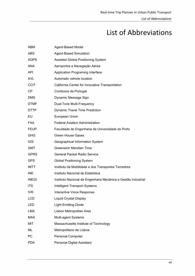
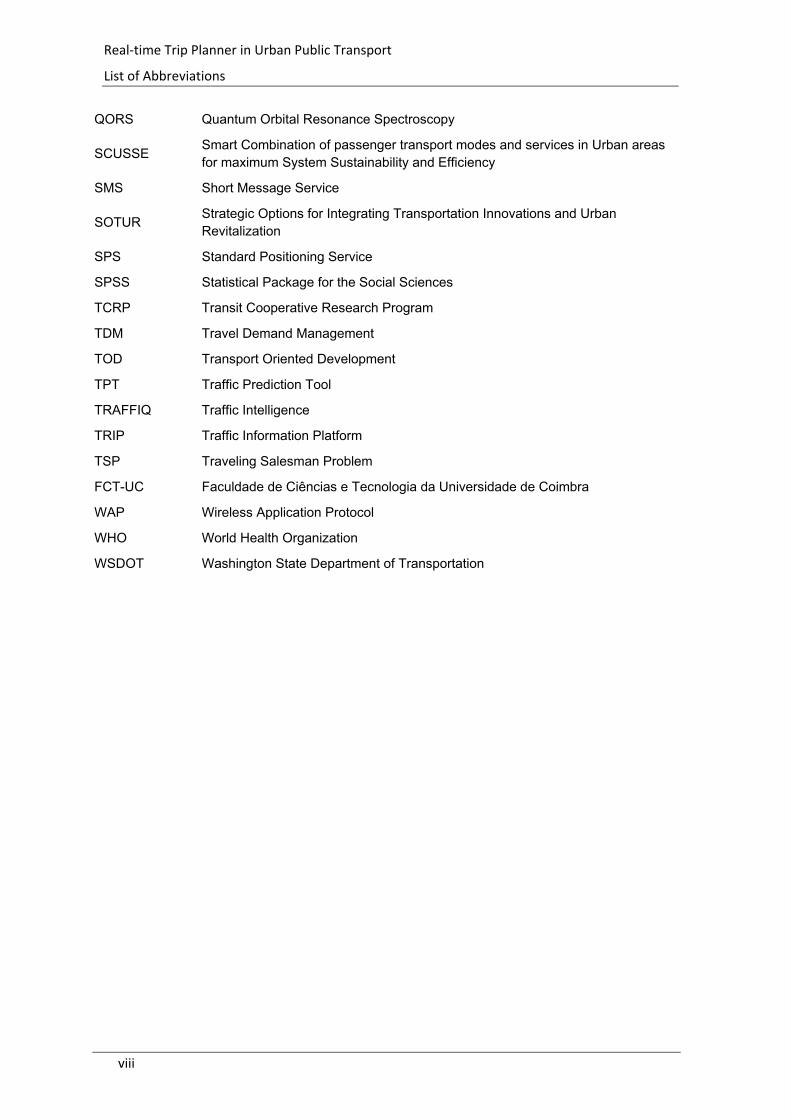
List of Abbreviations


ABM Agent-Based Model

ABS Agent-Based Simulation

AGPS Assisted Global Positioning System

ANA Aeroportos e Navegação Aérea

API Application Programing Interface

AVL Automatic vehicle location

CCIT California Center for Innovative Transportation

CP Comboios de Portugal

DMS Dynamic Message Sign

DTMF Dual-Tone Multi-Frequency

DTTP Dynamic Travel Time Prediction

EU European Union

FAA Federal Aviation Administration

FEUP Faculdade de Engenharia da Universidade do Porto

GHG Green House Gases

GIS Geographical Information System

GMT Greenwich Meridian Time

GPRS General Packet Radio Service

GPS Global Positioning System

IMTT Instituto da Mobilidade e dos Transportes Terrestres

INE Instituto Nacional de Estatística

INEGI Instituto Nacional de Engenharia Mecânica e Gestão Industrial

ITS Intelligent Transport Systems

IVR Interactive Voice Response

LCD Liquid Crystal Display

LED Light Emitting Diode

LMA Lisbon Metropolitan Area

MAS Multi-agent Systems

MIT Massachusetts Institute of Technology

ML Metropolitano de Lisboa

PC Personal Computer

PDA Personal Digital Assistant

viii



QORS Quantum Orbital Resonance Spectroscopy

SCUSSE Smart Combination of passenger transport modes and services in Urban areas for maximum System Sustainability and Efficiency

SMS Short Message Service

SOTUR Strategic Options for Integrating Transportation Innovations and Urban Revitalization

SPS Standard Positioning Service

SPSS Statistical Package for the Social Sciences

TCRP Transit Cooperative Research Program

TDM Travel Demand Management

TOD Transport Oriented Development

TPT Traffic Prediction Tool

TRAFFIQ Traffic Intelligence

TRIP Traffic Information Platform

TSP Traveling Salesman Problem

FCT-UC Faculdade de Ciências e Tecnologia da Universidade de Coimbra

WAP Wireless Application Protocol

WHO World Health Organization

WSDOT Washington State Department of Transportation

ix


Table of Contents

Table of Contents

Abstract ......................................................................................................................................... i

Resumo ........................................................................................................................................ iii

Acknowledgements ...................................................................................................................... v

List of Abbreviations ................................................................................................................... vii

Table of Contents ......................................................................................................................... ix

Figures ........................................................................................................................................ xiii

Tables .......................................................................................................................................... xv

I Introduction ........................................................................................................................... 1

I.1 Motivation ...................................................................................................................... 1

I.2 Objectives ....................................................................................................................... 5

I.3 Research Questions ........................................................................................................ 6

I.4 Research Methodology and Structure of the Dissertation ............................................ 7

II State of the practice and state of the art ........................................................................... 9

II.1 State of the practice ....................................................................................................... 9

II.1.1 Introduction ............................................................................................................ 9

II.1.2 Current Devices and Mechanisms ........................................................................ 10

II.1.3 Some examples .................................................................................................... 14

II.1.4 Summary and Conclusions ................................................................................... 19

II.2 State of the art ............................................................................................................. 20

II.2.1 Introduction .......................................................................................................... 20

II.2.2 Current Methodologies ........................................................................................ 21

II.2.3 Summary and Conclusions ................................................................................... 26

III Case Study Presentation .................................................................................................. 29

III.1 Introduction .............................................................................................................. 29

III.2 Lisbon’s Public Transport System ............................................................................. 30

x


Table of Contents

III.2.1 Bus and Tram Networks ....................................................................................... 30

III.2.2 Subway Network .................................................................................................. 33

III.2.3 Taxis ...................................................................................................................... 34

III.3 Conclusions ............................................................................................................... 35

IV Carris Log‐file Data Mining ............................................................................................... 37

IV.1 Introduction .............................................................................................................. 37

IV.2 Data description ....................................................................................................... 37

IV.2.1 Introduction .......................................................................................................... 37

IV.2.2 Attributes .............................................................................................................. 38

IV.3 Data Mining .............................................................................................................. 38

IV.3.1 Introduction .......................................................................................................... 38

IV.3.2 Stops Identification............................................................................................... 39

IV.3.3 Stops Aggregation ................................................................................................ 39

IV.3.4 Variables Deduction ............................................................................................. 40

IV.3.5 Outlier Filtering .................................................................................................... 42

IV.3.6 Route Establishment ............................................................................................ 42

IV.4 Spatial‐Temporal Assessment of the Speed Data .................................................... 43

IV.4.1 Overall Analysis .................................................................................................... 43

IV.4.2 Data Partitioning .................................................................................................. 44

IV.4.3 Zoning of the Study Area ...................................................................................... 50

IV.5 Conclusions ............................................................................................................... 51

V Simulation Model of Bus and Tram Operation ................................................................. 53

V.1 Introduction .................................................................................................................. 53

V.2 Simulation Framework ................................................................................................. 54

V.3 Model Description ........................................................................................................ 56

V.3.1 Description of the Active Objects ......................................................................... 57

V.3.2 Description of the Agents ..................................................................................... 62

xi


Table of Contents

V.3.3 Input Data of the Model ....................................................................................... 67

V.4 Computation of Travel Times in the Simulation Environment ..................................... 69

V.4.1 Generation of Speeds and Travel Times in the Simulation Environment ............ 69

V.4.2 Log‐File Speeds and Travel Times for the Simulation Environment ..................... 70

V.4.3 Prediction of Speeds and Travel Times in the Simulation Environment .............. 71

V.5 Evaluation of the travel time prediction model ........................................................... 75

V.5.1 Run the model for one day of the dataset ........................................................... 75

V.6 Conclusions................................................................................................................... 79

VI Trip‐Planner ...................................................................................................................... 81

VI.1 Introduction .............................................................................................................. 81

VI.2 Dijkstra Algorithm and Adaptations ......................................................................... 82

VI.3 Test the trip‐planner for short and medium term queries ...................................... 83

VI.3.1 Test for a synthetic population of clients to measure the agenda adjustment ... 83

VI.4 Conclusions ............................................................................................................... 86

VII Conclusions and Future Developments............................................................................ 87

References ................................................................................................................................. 91

xiii


Figures

Figures

Figure I.1 – Public service demand evolution (Carris 2010) ....................................................... 4

Figure I.2 – Dissertation structure ............................................................................................... 7

Figure II.1 – London DMS ........................................................................................................... 10

Figure II.2 – iBUS on‐bus LCD display ......................................................................................... 11

Figure II.3 – NextBus and similar operational scheme .............................................................. 13

Figure II.4 – New York City live traffic on Sep‐11‐2009 23:13 GMT ‐ Source: Google Maps ..... 13

Figure II.5 – New York City traffic prediction for a Friday 6:00 pm – Source: Google Maps ..... 14

Figure II.6 – Countdown operating schema ............................................................................... 15

Figure II.7 – Singapore Live Traffic website ............................................................................... 17

Figure II.8 – Search Box .............................................................................................................. 18

Figure II.9 – Avoid Traffic info .................................................................................................... 18

Figure II.10 – Report Incidents ................................................................................................... 18

Figure II.11 – A neuron cell (Heaton 2005) ................................................................................ 21

Figure II.12 – Example of a classification tree and solution space ............................................ 24

Figure III.1 – Lisbon’s Population evolution ............................................................................... 29

Figure III.2 – Transporlis website ............................................................................................... 30

Figure III.3 – Carris operating network map (Carris 2010) ........................................................ 31

Figure III.4 – Carris DMS ............................................................................................................ 31

Figure III.5 – Distance between stops analysis .......................................................................... 32

Figure III.6 – Subway network evolution ................................................................................... 33

Figure III.7 – Subway demand .................................................................................................... 33

Figure III.8 – Subway network map ‐ Source: (ML 2011) ........................................................... 34

Figure IV.1 – Summary flowchart .............................................................................................. 38

Figure IV.2 – Stops complete list ............................................................................................... 39

Figure IV.3 – Group creation ...................................................................................................... 40

Figure IV.4 – New variable computation ................................................................................... 40

Figure IV.5 – Route computation ............................................................................................... 43

Figure IV.6 – Daily speed profile of the complete network (Percentiles) .................................. 44

Figure IV.7 – Hierarchical clustering techniques ....................................................................... 45

Figure IV.8 – Information gain evaluation vs. number of clusters............................................. 46

Figure IV.9 – Spatial representation of the cluster analysis outputs ......................................... 47

xiv


Figures

Figure IV.10 –Daily speed profile of Cluster 1’s sections (Percentiles) ...................................... 48

Figure IV.11 – Daily speed profile of Cluster 2’s sections (Percentiles) ..................................... 48




Figure IV.15 – Map of the used traffic zoning ............................................................................ 50

Figure V.1 – Agent Based scheme .............................................................................................. 53

Figure V.2 – Conceptual model of the simulation ..................................................................... 55

Figure V.3 – Simulation Environment ........................................................................................ 56

Figure V.4 – Service Agent flowchart ......................................................................................... 63

Figure V.5 – User Agent flowchart ............................................................................................. 64

Figure V.6 – Section Agent flowchart ........................................................................................ 66

Figure V.7 – Process of computation of Instant Section Speed ................................................. 71

Figure V.8 – Prediction moment flowchart ................................................................................ 72

Figure V.9 – Regression schema ................................................................................................ 73

Figure V.10 – Build‐up concept .................................................................................................. 75

Figure V.11 – Estimated travel times median Section values versus Real travel times ............. 77

Figure V.12 ‐ Estimated travel times using Speed and Travel Time Prediction Model .............. 78

Figure V.13 ‐ Error frequency comparison ................................................................................. 79

Figure VI.1 ‐ Test Source/Destination Stops .............................................................................. 83

Figure VI.2 ‐ Trip‐planner error distribution .............................................................................. 85

xv


Tables

Tables

Table II.1 – State of the practice summary ................................................................................ 19

Table III.1 – Operating indicators comparison: 365 days working taxi ...................................... 35

Table IV.1 – Original variables ................................................................................................... 38

Table IV.2 – Computed variables ............................................................................................... 41

Table IV.3 – Number of sections in Clusters .............................................................................. 47

Table IV.4 – Summary of clusters analysis results ..................................................................... 51

Table V.1 – Features specification of the Route active object .................................................. 57

Table V.2 – Features specification of the Stop active object ..................................................... 57

Table V.3 – Features specification of the Groups active object ................................................ 58

Table V.4 – Features specification of the Common Section active object ................................ 58

Table V.5 – Features specification of the Street Path active object .......................................... 59

Table V.6 – Features specification of the Transfers active object ............................................. 59

Table V.7 – Features specification of the Zone active object .................................................... 59

Table V.8 – Features specification of the Census Block active object ....................................... 59

Table V.9 – Features specification of the Connectors active object.......................................... 60

Table V.10 – Features specification of the Pedestrian Network active object .......................... 60

Table V.11 – Features specification of the Nodes Transport Network active object ................ 60

Table V.12 – Features specification of the Transport Network active object ........................... 61

Table V.13 – Features specification of the Main active object .................................................. 61

Table V.14 – Features specification of other object classes ...................................................... 62

Table V.15 – Features specification of the Service agent .......................................................... 63

Table V.16 – Features specification of the User agent .............................................................. 64

Table V.17 – Features specification of the Section agent.......................................................... 66

Table V.18 – Description of the variables of the speed generation model ............................... 70

Table VI.1 ‐ Test indicators ........................................................................................................ 84

Table VI.2 ‐ Transporlis vs. Trip‐planner .................................................................................... 85

1


Introduction

I Introduction

I.1 Motivation

The world is increasingly urban and increasingly mobile. Today more than 50% of the world's

population lives in cities. In the European Union 80% of the population live in urban areas

(Herrero 2011).

As mobility is perceived in modern societies as a key element to ensure the access of citizens

to activities and goods, the growth of urban areas led to a significant increase in the complexity of

the transport systems to ensure safe and efficient mobility. These facts, along with the

democratization of car ownership, are producing a steady increase of the impacts of urban

mobility in modern cities (Banister 2008).

Although a great effort in increasing the quality of public transport supply has been carried

out worldwide to fight this fact, especially in the European context, the demand for collective

transport modes has been globally decreasing in the last decades in urban areas (Zegras and

Gakenheimer 2006).

This fact can be explained by the increasing complexity of urban mobility in developed and

emergent societies derived from uncoordinated land use and transport policies (urban sprawl),

changes in lifestyles and activity patterns and the increase of car ownership rates. All these

factors play an important role on the difficulty of public transport to deal efficiently with a

disperse time‐space demand, especially for low density urban areas.

These issues have been acknowledged by the main policy institutions, which have been trying

to invert this tendency through the introduction of measures in three different fronts:

Increase the attractiveness and competiveness of public transport supply by bringing

in new transport alternatives and introducing new Intelligent Transport Systems (ITS)

to support the system operation and upgrade the information to users from the

system (Taylor, Nozick et al. 1997); (Transport Demand Management ‐ TDM)1;

1 Transport demand management (TDM) is the application of strategies and policies to reduce travel demand (specifically that of single‐occupancy private vehicles), or to redistribute this demand in space or in time. These measures incorporate different fields, ranging from pricing to incorporation of technology.

2


Introduction

Introduce constraints to private car use through parking regulation and pricing, as

well as new road charging schemes (also within the scope of TDM measures) (Viegas

2001);

Create more sustainable land use patterns, demanding less car intensive use and

greater public transport accessibility (Cervero, Murphy et al. 2004) (Transport

Oriented Development – TOD)2.

From a land use perspective, urban design has observed, in the last decades, frequent

unregulated expansions of cities, which has been introducing complexity and inefficiency in public

transport networks. This is something that has been observed mainly in the so‐called developed

cities with a speculation or overestimation in terms of house prices in their historical center. This

fact has been leading medium and low social strata to move out to cheaper suburb locations, due

to the increasing recognition of the value of accessibility, producing significant effects of

gentrification, although, there are still low income areas within the traditional city boundaries

(Brueckner 2001). Besides the environmental and congestion problems that this fact entails, one

major consequence observed is the loss of competiveness of cities at a global scale (Cervero

2009).

Public transport use has also been affected by a perception bias of car users towards travel

costs. Especially after purchasing a car, only variable costs like fuel and parking fees are taken into

account, while public transport costs are always internalized. The neglect of fixed expenses, like

the purchase of the car and insurance, may bias considerably a direct comparison between the

charges of using a car versus a public transport service (Henley, Levin et al. 1981; Viegas 2010).

Information awareness may also play a relevant role in this complex equation. The

heterogeneity of target users (e.g. in age and level of education) may also be a barrier to access

information, especially for groups not familiar with new technologies. Furthermore, the

development of a public transport culture among teenagers who are starting to exert their

mobility independence, may also be a key factor to encourage them to use public transport (Lyons

and Harman 2002).

2 A transit‐oriented development (TOD) is a mixed‐use residential or commercial area designed to maximize access to public transport, and often incorporates features to encourage transit ridership, being located close to a large public transport station (subway, rail or light‐rail).

3


Introduction

One direct consequence of the loss of competiveness of public transportation against the

private car is the increase of mobility externalities, especially greenhouse gas emissions (GHG)

and other pollutants, which affect the quality of life of citizens in urban areas. The World Health

Organization estimated 1,900 deaths per year in Portugal only due to outdoor air pollution (WHO

2007).

Transport systems should be subject to the rationality of current energy and environmental

requirements in order to comply with the new paradigms of sustainability. They face significant

challenges to mitigate the external impacts of mobility on the environment and human health,

especially in highly motorized societies that shape their urban design in light of a car dependent

paradigm (Herrero 2011).

The reduction of urban congestion problems will benefit businesses and citizens in different

ways such as reducing costs, saving time and improving accessibility. Furthermore a decreased

dependence on fossil fuels allows a reduction in greenhouse gases emission levels which

contribute to an overall increase in inhabits life quality.

Interventions on the public transport design and operation are paramount to target urban

congestion reduction. Yet, improvements to public transport operations alone will not necessarily

persuade people to forego the use of their cars and make use of public transport modes.

Intending travelers need to be informed of what is available (Lyons and Harman 2002).

Two of the main reasons why public transport systems are incapable of captivating

passengers are the lack of reliability and information regarding the service that they wish to

consume right away. According to Lyons & Harman, the major grievances regarding public

transportation are often delays in the arrival of buses and trains and the excessive time on board

due to unforeseen events such as accidents or traffic. While some passengers complain about

these incidents others “view those types of irritations quite fatalistically” (2003).

Typically, passengers value the information about the best routes to take and the travel times

associated with each one, so that they can eliminate any possible contingencies such as traffic or

intermodal waiting times. While in public transport, passengers often feel less secure especially

when travelling through unknown routes. To circumvent this fact, information on board should be

available to the passenger. In case of trip interruption due to some sort of incident, that kind of

information would allow passengers in an unknown location to considerate alternatives to

continue their journey (Beirao and Cabral 2007).

4


Introduction

As demonstrated in the TCRP Report 92 (2003), with real‐time information displayed:

Passengers felt that waiting for the bus was more acceptable;

Passengers found that time seemed to pass more quickly when they knew how long

their wait would be;

The actual bus service was perceived as being more reliable;

Of those passengers traveling late hours, waiting at night was perceived as being

safer;

Passengers general feelings improved toward bus travel, the particular operator, and

London Transport;

Travelers are mainly concerned with their own particular journeys. Therefore, targeting

information provision as far as possible is essential. This should include information on travel

options: e.g. faster and more expensive against cheaper and slower (Lyons and Harman 2002).

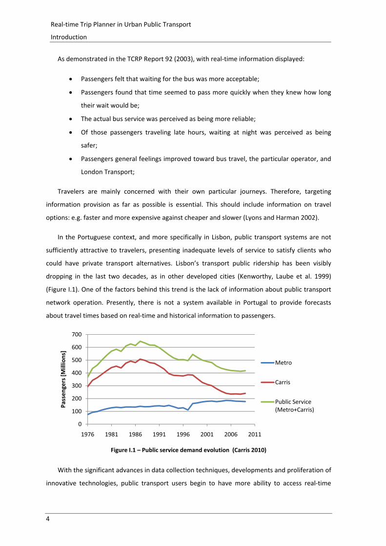
In the Portuguese context, and more specifically in Lisbon, public transport systems are not

sufficiently attractive to travelers, presenting inadequate levels of service to satisfy clients who

could have private transport alternatives. Lisbon’s transport public ridership has been visibly

dropping in the last two decades, as in other developed cities (Kenworthy, Laube et al. 1999)

(Figure I.1). One of the factors behind this trend is the lack of information about public transport

network operation. Presently, there is not a system available in Portugal to provide forecasts

about travel times based on real‐time and historical information to passengers.

Figure I.1 – Public service demand evolution (Carris 2010)

With the significant advances in data collection techniques, developments and proliferation of

innovative technologies, public transport users begin to have more ability to access real‐time

0

100

200

300

400

500

600

700

1976 1981 1986 1991 1996 2001 2006 2011

Passengers [Millions]

Metro

Carris

Public Service (Metro+Carris)

5


Introduction

information that helps the selection of routes in advance or during a trip. With accurate and

reliable information, travelers can make decisions to avoid network segments that are congested,

or in the context of public transport, choose the set of lines that allow reaching the destination in

the shortest time. Users are beginning to be able to make changes in departure times that allow

an optimal overall travel time and in some cases ponder different arrival times when the decrease

in the overall travel time is significant (Ishak and Alecsandru 2004).

Nowadays geo‐location systems, gadgets and mobile data services are increasingly present in

citizen’s routines. Combining different mobile services with existing transport systems can

improve the quality of Automatic Vehicle Location (AVL) services and may help changing the

perception of citizens towards public transports.

As mentioned by the European Commission (2011) in the White Paper on Transport Policy

“curbing mobility is not an option” and therefore this study attempts to evaluate and test the

possibility of creating a decision‐support system for passengers on public transportation that

helps to choose the best route to take and which are the expected arrival times do destinations.

By doing so, the system would try to reduce the constant uncertainty about travel times and

intermodal waiting times. By answering to questions like:

Which public transport routes are available for my trip?

Which route or combination of routes gets me there earliest? And with fewer

transfers?

This could create conditions for public transport to become more attractive to individual

transport users, especially for non‐regular users of the system that alternate from mode to mode

depending on their daily agendas and destinations. And, more importantly, it would build

confidence on the service provided, which is a key element to retain customers (and attract new

customers) in all types of services.

I.2 Objectives

This dissertation intends to develop a model for a real‐time information tool, which will allow

users to plan their immediately subsequent journeys through reliable information about the

public transport supply, presenting the best options in terms of optimized route, optimized travel

time and possible delays caused by accidents or incidents.

6


Introduction

The tool basis when applied in practice is the real‐time exchange of data between a personal

mobile device like a mobile phone, personal digital assistant (PDA), tablet or similar and the public

transport network with the required data processing being remotely done by a system central.

Current time being known to the machines involved in this dialogue, the main inputs expected

are the current passenger location and his intended destination, with the underlying assumption

that the trip is to start as soon as possible. The main outputs are a small set of suggestions in

terms of overall route, pedestrian paths and bus or tramway lines involved, specifying transfer

points (if they exist) with the associated arrival times at the destination and at those transfer

points, all in real‐time. The walking speed of the user is important to establish feasible paths and

should initially be declared or a default value taken. This could preferably be subsequently

calibrated by GPS‐based automatic calculations when the tool is used.

This tool would ideally be customizable by declaration of the users preferences (for instance

minimize transfers even if trip duration is increased by no more than 10 minutes), on the basis of

which the small set of suggestions would be ranked by decreasing order of preference.

This dissertation aims to develop and test a real‐time trip planner for passengers based on the

Lisbon bus network operated by the company Carris.

I.3 Research Questions

This dissertation tries to address the feasibility, reliability and added‐value of providing

accurate real‐time information and path recommendations for the immediate use of the public

transport system, reducing the negative effect of the current uncertainty about the service that

will be delivered. This study aims to address and answer some relevant questions about this

matter from theoretical and application perspectives.

From a theoretical point of view, this dissertation will address:

Which data is required for a reliable real‐time prediction system?

Which algorithms are adequate to process it?

How to produce real‐time predictions of the network travel times under different

circumstances?

How accurate and reliable can this system be?

The developed application will also try to assess:

7


Introduction

Will the system be able to provide accurate trip‐plans to travelers?

All these questions will be addressed in this dissertation, having a special focus on the

methodological formulation required for a future real world application that would allow

enhancing the performance of the public transport system.

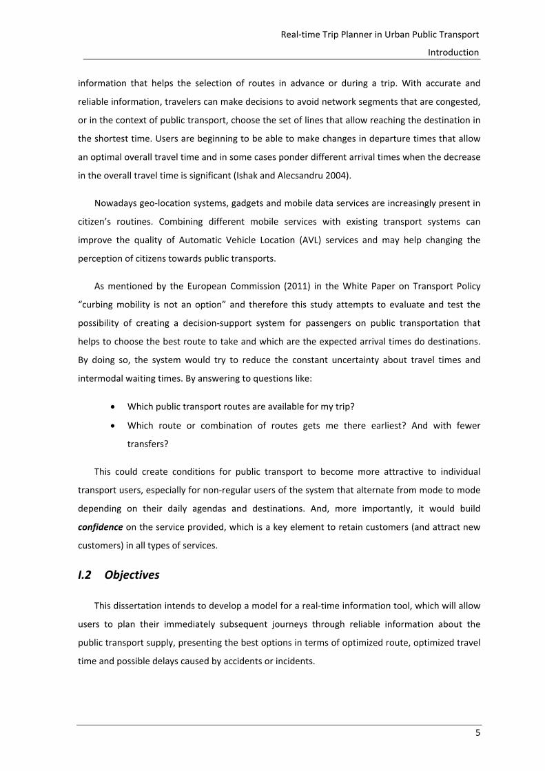
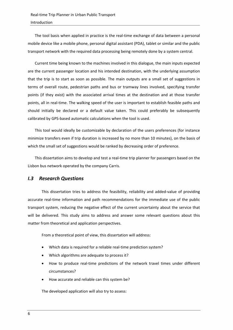
I.4 Research Methodology and Structure of the Dissertation

The current study aims to answer the above questions firstly by contextualizing the objectives

with the systems already in operation around the world and with the research that is already

being developed using different mathematical models of pattern recognition and prediction. The

Lisbon case study is presented and a methodology is chosen to develop a model, taking into

consideration the available data. This model is then tested and discussed and finally future

development works are proposed. The structure and articulation of the different parts of the

work can be found in a graphical representation in Figure I.2.

Figure I.2 – Dissertation structure

Chapter II sets out to describe the already operational systems on some reference cities

around the world, with a particular emphasis on European and American cities. It also states what

types of information those systems provide to the end user, in which physical support they are

presented and when that information is available, which models or techniques are used to

process data and model forecasts. The same chapter presents some aspects of data mining

concepts, and why these techniques are useful in the context of urban traffic forecasting.

8


Introduction

The purpose of Chapter III is to present the targeted study area, the main transport modes

available and characteristics of each network associated with the correspondent mode. Even if

superficially, the chapter will describe and try to evaluate the performance of the bus network in

terms of its reliability and ability to generate demand from potential users.

Then, Chapter IV describes the data used in this study, provided by the bus and tramway

public transport operator in Lisbon Carris. It will assess what are the dimensions of the data set,

its attributes and how this information was processed for the calibration of speeds required to

characterize the sections that constitute the urban road network in evaluation.

Chapter V presents a real‐time estimation model for travel times in Lisbon’s public bus and

tramway network integrated in a simulation model environment, using an Agent‐based

formulation. It will be discussed the used methodology to predict travel times, how the estimates

are made for each segment of the network as well as an analysis of the system’s performance.

Chapter VI presents the trip planner application based on the developed travel time

prediction model. This chapter includes the formulation and design of an information system for

public transport users and measures the reliability of plans transmitted to users. The model

presented aims to set the basis for a development of a future real application using the available

communication technologies.

Finally, conclusions drawn from this study are presented and future development works are

proposed in Chapter VII.

9


State of the practice and state of the art

II State of the practice and state of the art

II.1 State of the practice

II.1.1 Introduction

Real‐time Information Systems are becoming essential tools within the ITS field. Their purpose

is to better inform customers and operational authorities of the transport system condition. From

a customer perspective, these systems may support decisions related with transport mode, routes

and expected travel times. To authorities these tools may allow a better knowledge of traffic

conditions, eventual incidents or accidents, leading to improved real time management of the

services provided (Battelle 2002).

Many Real‐time Information Systems are based on Global Positioning System (GPS). This

system associated with geo‐referenced maps has allowed the development of many other

systems and technologies for traffic prediction. The use of the GPS to support real‐time

information relies on the high degree of accuracy at reduced costs. Real‐world data collected by

the Federal Aviation Administration (FAA) show that some high‐quality GPS SPS (SPS stands for

Standard Positioning Service, the civilian GPS service) receivers currently provide better than 3

meter horizontal accuracy (2011).

This accuracy can even be optimized when augmentation technologies are associated to the

devices like Assisted GPS (AGPS). AGPS is a technology that uses an extra positioning instrument

besides satellites: a mobile network tower that helps to triangulate a GPS equipped device

localization.

In this chapter, we will address the communication technologies used to provide real time

information, as well as the underlying data processing of traffic prediction. Nowadays this real‐

time data integration can already be automatically performed by distributed traffic detection

machines or by user feedback.

10



II.1.2 Current Devices and Mechanisms

II.1.2.1 Dynamic Message Signs

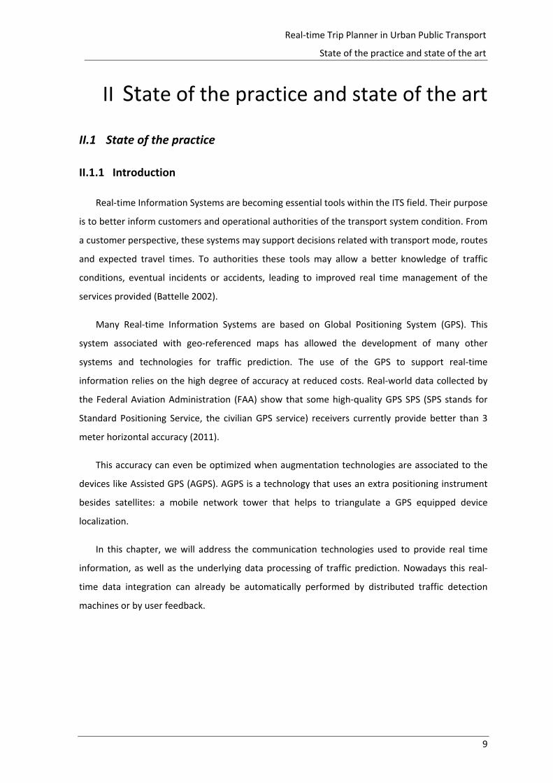
A Dynamic Message Sign (DMS) is a panel that can show words, numbers or symbols,

dynamically changed from a remote location. The most common display technology is based on

Light‐Emitting Diodes (LED) (see Figure II.1.).

This type of information instrument has been mainly implemented on highways or freeways,

playing an important role in road safety and traffic operations. The signs are usually light devices

whose objective is to capture road users attention (WSDT and Publications 2004). As the message

type can be variable, DMSs in this kind of infrastructure can be used to display different posts

such as:

Traffic restrictions or traffic prohibition in some part of a road/bridge/tunnel;

Weight, width or height restrictions;

Broken vehicles or accidents;

Weather and road conditions;

Local events;

Construction and maintenance of roads;

Traffic congestion;

Waiting time expected in traffic queue.

In public transport systems, DMSs are normally used to provide information on expected

arrival and departure time of buses and rails at stops or stations. The main purpose of these

systems is to increase the reliability of public transport schedules to users. Typically waiting times

for buses are provided through countdown timers.

Figure II.1 – London DMS

11



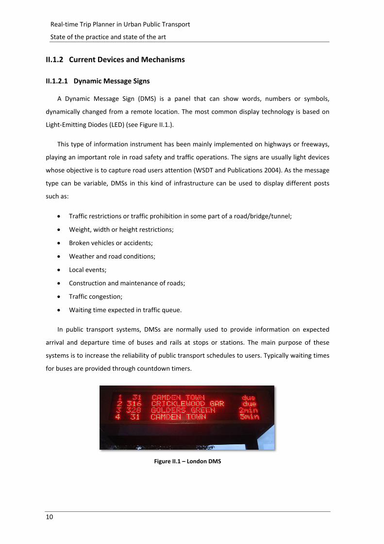
Transport for London (TfL) implemented an integrated AVL project in its bus service. The

system called iBus (Figure II.2) combines several technologies such as GPS and map matching with

inputs from a gyroscope and speedometer. It also uses General Packet Radio Service (GPRS) to

send the location of each bus every 30 seconds to a computer central system that processes data

and broadcasts to different media supports.

Figure II.2 – iBUS on‐bus LCD display

iBus service makes traveling easier for (TfL 2011):

Visually or hearing‐impaired passengers;

Infrequent travelers;

Passengers facing language barriers;

People travelling in an unfamiliar area.

It also helps to enhance bus arrivals countdowns shown in DMSs whose operation

mechanisms will be detailed in section II.1.3.2 of this dissertation.

II.1.2.2 Interactive Voice Response

Interactive Voice Response (IVR) is a technology that allows a computer to detect voice and

Dual‐Tone Multi‐Frequency (DTMF) during a phone call.

IVR systems talk to callers following a recorded script. It prompts a response from the client to

respond either verbally or by pressing a touchtone key and supplies the customer with

information based on pre‐recorded responses (Human Resources Software 2007).

A 2005 study from Washington State Department of Transportation (WSDOT) showed the

success of its IVR system.

In the 1990s WSDOT launched a highway hotline that provided information about the state of

highway road conditions, scheduled constructions, and mountain pass conditions. That system

12



evolved and was the first to be associated with the American national traffic information number

511. Nowadays, Washington State’s 511 system provides voice‐driven access to real‐time traffic

reports, continually updated roadway incident and construction information, express‐lane status,

mountain‐pass road conditions, and weather information. It even took a multi modal approach by

connecting callers directly to the state’s ferry system and providing phone numbers for transit,

passenger rail, and airlines.

WSDOT noted that if a person dials 511 from an environment where background noise exists

(such as a car), the 511 system has a difficult time separating the speech from the background

sounds. This led to customer frustration, and so, in November 2004, WSDOT introduced a touch‐

tone option.

In the same report it is stated that an overall 71% of respondents indicated that the

information they sought did not drive them to change their travel plans. However, those

respondents looking for information on Seattle specific area roads and freeways were slightly

more likely to change their travel plans than those looking for information on roads in the rest of

the state.

In this context, a 21% reported change in travel behavior is highly significant, which may have

already some considerable benefits in highly congested areas. If all drivers dialed 511 and

followed the same pattern, significant improvement in traffic management could be achieved.

Only 12% of respondents claimed that the information provided was not accurate and 10%

stated that the system did not provide the needed information.

Almost all the survey respondents (87%) agreed that they would be likely or very likely to use

the 511 system again (WSDT 2005).

Respondents were generally satisfied with the 511 features, except for the voice recognition

feature. Taking into account that this study refers to 2005 and that voice recognition techniques

have been in constant development, it is expected that a new 2011 survey would reveal better

feedback.

II.1.2.3 Internet and Mobile devices

With the widespread of Internet and smartphones there are several emerging information

systems that provide real‐time forecasts online. One of these systems currently operating is

NextBus.

13



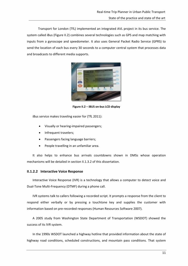
NextBus was developed by NextBus, Inc. and works not only with buses but also with trams,

light rail and other surface vehicles. Each vehicle uses the global positioning satellites and

transmits its location and speed to a database. Given the current position of the bus, the path and

typical traffic patterns, the system estimates the arrival of vehicles to stops (NextBus Inc. 2011).

Figure II.3 – NextBus and similar operational scheme

The information is then made available at bus and tram stops with DMSs and on the Internet

becoming accessible by computers and handheld devices such as tablet computers or cell phones.

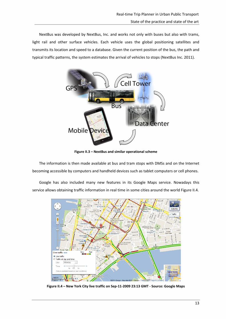
Google has also included many new features in its Google Maps service. Nowadays this

service allows obtaining traffic information in real time in some cities around the world Figure II.4.

Figure II.4 – New York City live traffic on Sep‐11‐2009 23:13 GMT ‐ Source: Google Maps

14



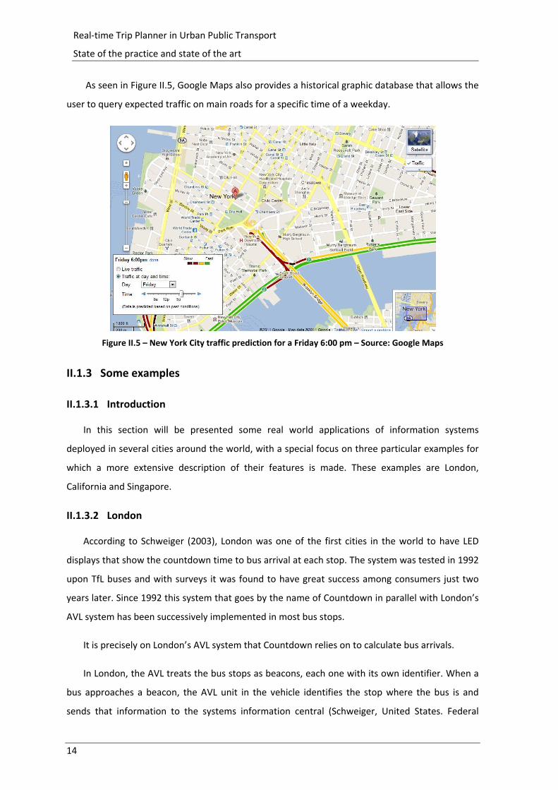
As seen in Figure II.5, Google Maps also provides a historical graphic database that allows the

user to query expected traffic on main roads for a specific time of a weekday.

Figure II.5 – New York City traffic prediction for a Friday 6:00 pm – Source: Google Maps

II.1.3 Some examples

II.1.3.1 Introduction

In this section will be presented some real world applications of information systems

deployed in several cities around the world, with a special focus on three particular examples for

which a more extensive description of their features is made. These examples are London,

California and Singapore.

II.1.3.2 London

According to Schweiger (2003), London was one of the first cities in the world to have LED

displays that show the countdown time to bus arrival at each stop. The system was tested in 1992

upon TfL buses and with surveys it was found to have great success among consumers just two

years later. Since 1992 this system that goes by the name of Countdown in parallel with London’s

AVL system has been successively implemented in most bus stops.

It is precisely on London’s AVL system that Countdown relies on to calculate bus arrivals.

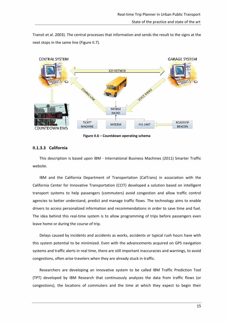
In London, the AVL treats the bus stops as beacons, each one with its own identifier. When a

bus approaches a beacon, the AVL unit in the vehicle identifies the stop where the bus is and

sends that information to the systems information central (Schweiger, United States. Federal

15



Transit et al. 2003). The central processes that information and sends the result to the signs at the

next stops in the same line (Figure II.7).

Figure II.6 – Countdown operating schema

II.1.3.3 California

This description is based upon IBM ‐ International Business Machines (2011) Smarter Traffic

website.

IBM and the California Department of Transportation (CalTrans) in association with the

California Center for Innovative Transportation (CCIT) developed a solution based on intelligent

transport systems to help passengers (commuters) avoid congestion and allow traffic control

agencies to better understand, predict and manage traffic flows. The technology aims to enable

drivers to access personalized information and recommendations in order to save time and fuel.

The idea behind this real‐time system is to allow programming of trips before passengers even

leave home or during the course of trip.

Delays caused by incidents and accidents as works, accidents or typical rush hours have with

this system potential to be minimized. Even with the advancements acquired on GPS navigation

systems and traffic alerts in real time, there are still important inaccuracies and warnings, to avoid

congestions, often arise travelers when they are already stuck in traffic.

Researchers are developing an innovative system to be called IBM Traffic Prediction Tool

(TPT) developed by IBM Research that continuously analyzes the data from traffic flows (or

congestions), the locations of commuters and the time at which they expect to begin their

16



journeys. With this information, scientists hope they can provide recommendations in real time

regarding which metro, train stations or bus stops are closer to them and even inform if there is

the possibility for the commuter to park at each station.

One of the most important principles of intelligent transport systems in this context is that

information reaches the users before they are stuck in traffic and thus can adjust their travel

decisions.

The aforementioned TPT system was tested in Singapore where local authorities responsible

for traffic control in association with IBM hope to acquire information about traffic conditions

with an hour in advance. The system combines information collected from video cameras, GPSs,

devices in taxis and sensors embedded in city streets.

The average volumes of traffic and circulation speeds are the keys to the characterization of

traffic. In ideal conditions, information about traffic volume and speed must be continuously

monitored and recorded through multiple and different detectors. According to Min (2007) “TPT’s

goal is to provide fine‐time resolution and near‐term prediction of average volume and speed

across every link in a road network”.

The traffic conditions are measured by average time observed in different types of vehicles

operating on public roads (the different traffic participants).That said it used a statistical approach

that credits the "law of large numbers." Some researchers throughout history have revealed they

have doubts about the ability to predict traffic advocating that traffic follows a "chaotic behavior".

Studies have shown otherwise.

The model used by IBM is based on two main components:

Capture trends

Measure the deviation from trend

The spatio‐temporal relationship is an essential aspect of road traffic prediction. The

fundamental observation is that the traffic condition at a link is affected by the immediate past

traffic conditions of some number of its neighboring links (Wynter and Min 2011).

Scientists established a spatial‐temporal model motivated by the serial correlation and spatial

correlation present in traffic data. The model is comparable to models of water flow over a

network. Through model selection criteria, they ascertained the number of neighboring locations

17



that have a significant effect on local traffic patterns. They then obtained the order of serial

correlation by using the same data.

The model was recalibrated at the beginning of each week on data from the most recent six

weeks. The updated model can be used to perform real‐time forecasting throughout the week

(Min 2007). Scientists believe they are involved in the development of an accurate, fast and wide

system that covers most of the complex road network. There is strong expectation that the

system will be essential in the future of planning urban road systems and commuter’s routines.

Unfortunately, there is little information available to the public other than the system that is

already online and running for use.

II.1.3.4 Singapore

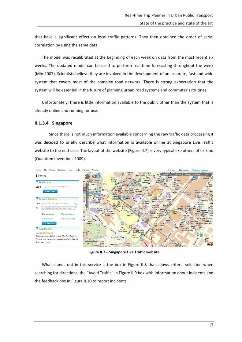
Since there is not much information available concerning the raw traffic data processing it

was decided to briefly describe what information is available online at Singapore Live Traffic

website to the end‐user. The layout of the website (Figure II.7) is very typical like others of its kind

(Quantum Inventions 2009).

Figure II.7 – Singapore Live Traffic website

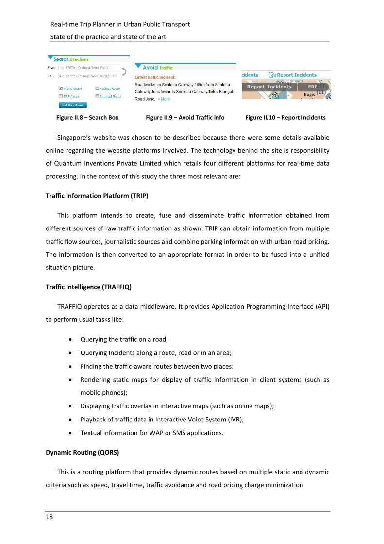
What stands out in this service is the box in Figure II.8 that allows criteria selection when

searching for directions, the “Avoid Traffic” in Figure II.9 box with information about incidents and

the feedback box in Figure II.10 to report incidents.

18



Figure II.8 – Search Box Figure II.9 – Avoid Traffic info Figure II.10 – Report Incidents

Singapore’s website was chosen to be described because there were some details available

online regarding the website platforms involved. The technology behind the site is responsibility

of Quantum Inventions Private Limited which retails four different platforms for real‐time data

processing. In the context of this study the three most relevant are:

Traffic Information Platform (TRIP)

This platform intends to create, fuse and disseminate traffic information obtained from

different sources of raw traffic information as shown. TRIP can obtain information from multiple

traffic flow sources, journalistic sources and combine parking information with urban road pricing.

The information is then converted to an appropriate format in order to be fused into a unified

situation picture.

Traffic Intelligence (TRAFFIQ)

TRAFFIQ operates as a data middleware. It provides Application Programming Interface (API)

to perform usual tasks like:

Querying the traffic on a road;

Querying Incidents along a route, road or in an area;

Finding the traffic‐aware routes between two places;

Rendering static maps for display of traffic information in client systems (such as

mobile phones);

Displaying traffic overlay in interactive maps (such as online maps);

Playback of traffic data in Interactive Voice System (IVR);

Textual information for WAP or SMS applications.

Dynamic Routing (QORS)

This is a routing platform that provides dynamic routes based on multiple static and dynamic

criteria such as speed, travel time, traffic avoidance and road pricing charge minimization

19



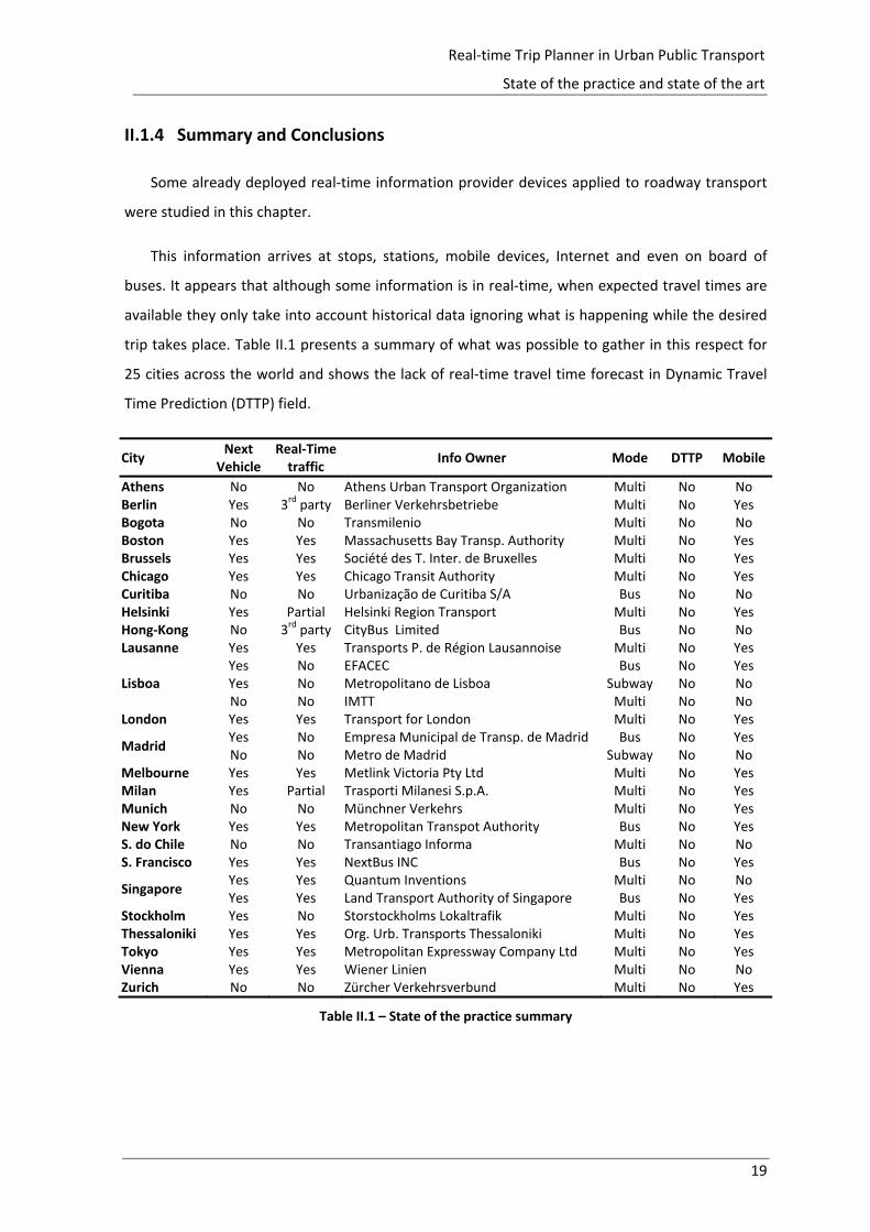
II.1.4 Summary and Conclusions

Some already deployed real‐time information provider devices applied to roadway transport

were studied in this chapter.

This information arrives at stops, stations, mobile devices, Internet and even on board of

buses. It appears that although some information is in real‐time, when expected travel times are

available they only take into account historical data ignoring what is happening while the desired

trip takes place. Table II.1 presents a summary of what was possible to gather in this respect for

25 cities across the world and shows the lack of real‐time travel time forecast in Dynamic Travel

Time Prediction (DTTP) field.

City Next

Vehicle Real‐Time traffic

Info Owner Mode DTTP Mobile

Athens No No Athens Urban Transport Organization Multi No NoBerlin Yes 3rd party Berliner Verkehrsbetriebe Multi No YesBogota No No Transmilenio Multi No NoBoston Yes Yes Massachusetts Bay Transp. Authority Multi No YesBrussels Yes Yes Société des T. Inter. de Bruxelles Multi No YesChicago Yes Yes Chicago Transit Authority Multi No YesCuritiba No No Urbanização de Curitiba S/A Bus No NoHelsinki Yes Partial Helsinki Region Transport Multi No YesHong‐Kong No 3rd party CityBus Limited Bus No NoLausanne Yes Yes Transports P. de Région Lausannoise Multi No Yes

Lisboa Yes No EFACEC Bus No YesYes No Metropolitano de Lisboa Subway No NoNo No IMTT Multi No No

London Yes Yes Transport for London Multi No Yes

Madrid Yes No Empresa Municipal de Transp. de Madrid Bus No YesNo No Metro de Madrid Subway No No

Melbourne Yes Yes Metlink Victoria Pty Ltd Multi No YesMilan Yes Partial Trasporti Milanesi S.p.A. Multi No YesMunich No No Münchner Verkehrs Multi No YesNew York Yes Yes Metropolitan Transpot Authority Bus No YesS. do Chile No No Transantiago Informa Multi No NoS. Francisco Yes Yes NextBus INC Bus No Yes

Singapore Yes Yes Quantum Inventions Multi No NoYes Yes Land Transport Authority of Singapore Bus No Yes

Stockholm Yes No Storstockholms Lokaltrafik Multi No YesThessaloniki Yes Yes Org. Urb. Transports Thessaloniki Multi No YesTokyo Yes Yes Metropolitan Expressway Company Ltd Multi No YesVienna Yes Yes Wiener Linien Multi No NoZurich No No Zürcher Verkehrsverbund Multi No Yes

Table II.1 – State of the practice summary

20



II.2 State of the art

II.2.1 Introduction

The traffic predicting systems have the potential to enhance traffic conditions and reduce

delays by improving the utilization of the available capacity. These systems exploit existing

technological advances in terms of computing, communication capabilities and capacity of

monitoring and control traffic transport networks. These systems also incorporate various levels

of traffic information in order to be able to dynamically advise travelers in terms of mode, path

selection and timing for travel plans.

The successful implementation of information technology systems in transport is dependent

on the degree of resolution and timing of sensing traffic conditions. These systems are expected

to use advanced models that analyze the different data available, preferably in real‐time and from

different sources, to estimate and predict traffic conditions.

It is important to distinguish the different traffic prediction systems or models. In the context

of this study they are manly distinguished by their purpose. On one hand, there are conventional

models that aim to predict the evolution of traffic in medium and long term, while in the other,

short term forecast models are used for management and operational control (Afandizadeh and

Kianfar 2009).

One characteristic of traffic prediction systems is the enormous amount of data required to

produce accurate estimates. To deal with such an amount of data it is paramount to use data

mining procedures to reduce complexity and allow a better understanding of all the underlying

phenomena. According to Clifton (2011) “Data mining, also called knowledge discovery in

databases in computer science, is the process of discovering interesting and useful patterns and

relationships in large volumes of data“. To achieve those patterns and relationships there are

several different approaches or methodologies that can be applied. While it is impossible to

describe all of them in this document, the most important ones in the context of this work are

going to be lightly explored.

21



II.2.2 Current Methodologies

II.2.2.1 Neural Networks

A neural network is a highly interconnected structure of computing units, often called

neurons, capable of learning. In a neural network, knowledge is acquired from an environment

through a process of learning and is stored in the links between the computational units (Cortez

and Neves 2000).

A computer can do mathematical calculations much faster than the human brain. Although it

is much faster in arithmetic information processing, it is extremely difficult for a computer to

differentiate a cat from a dog in an image, something that a two year child can do in a second.

The neural network designation derives from their mathematical formulation, which tries to

mimic the human way of thinking. Since the human brain is too complex and therefore difficult to

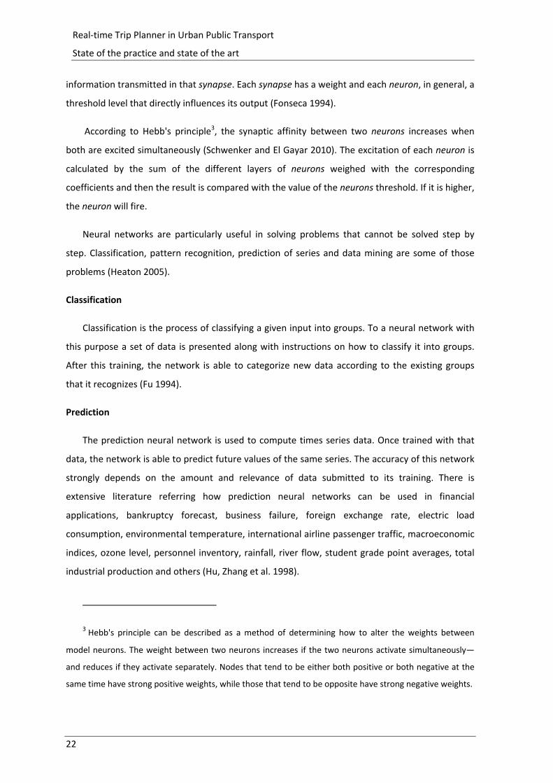
model, neural networks attempt to imitate the brain constituents, neurons (Figure II.11).

Figure II.11 – A neuron cell (Heaton 2005)

The neuron is formed by cell body and several branches. The branches are called dendrites

and transmit information from neurons ends to the central body. There is also usually a core

branch that is named axon that transmits signals from the cell body to its extremities. The

extremes of the axon are connected with dendrites of other neurons by synapses. In many cases,

the axon is directly connected with other axons or with the body of another neuron (Barreto

2002).

The synapses play a key role in the memorization of information. In the human brain, the

amount of neurotransmitters released by a synapse during an axon pulse represents the

22



information transmitted in that synapse. Each synapse has a weight and each neuron, in general, a

threshold level that directly influences its output (Fonseca 1994).

According to Hebb's principle3, the synaptic affinity between two neurons increases when

both are excited simultaneously (Schwenker and El Gayar 2010). The excitation of each neuron is

calculated by the sum of the different layers of neurons weighed with the corresponding

coefficients and then the result is compared with the value of the neurons threshold. If it is higher,

the neuron will fire.

Neural networks are particularly useful in solving problems that cannot be solved step by

step. Classification, pattern recognition, prediction of series and data mining are some of those

problems (Heaton 2005).

Classification

Classification is the process of classifying a given input into groups. To a neural network with

this purpose a set of data is presented along with instructions on how to classify it into groups.

After this training, the network is able to categorize new data according to the existing groups

that it recognizes (Fu 1994).

Prediction

The prediction neural network is used to compute times series data. Once trained with that

data, the network is able to predict future values of the same series. The accuracy of this network

strongly depends on the amount and relevance of data submitted to its training. There is

extensive literature referring how prediction neural networks can be used in financial

applications, bankruptcy forecast, business failure, foreign exchange rate, electric load

consumption, environmental temperature, international airline passenger traffic, macroeconomic

indices, ozone level, personnel inventory, rainfall, river flow, student grade point averages, total

industrial production and others (Hu, Zhang et al. 1998).

3 Hebb's principle can be described as a method of determining how to alter the weights between

model neurons. The weight between two neurons increases if the two neurons activate simultaneously—

and reduces if they activate separately. Nodes that tend to be either both positive or both negative at the

same time have strong positive weights, while those that tend to be opposite have strong negative weights.

23



Pattern Recognition

As the name suggests, pattern recognition networks are used to differentiate or aggregate

data sets. They can help to solve important problems in a variety of engineering and scientific

disciplines such as biology, psychology, medicine, marketing, computer vision, artificial

intelligence, and remote sensing. A pattern to be recognized can be a fingerprint image, a

handwritten cursive word, a human face, or a speech signal (e.g. when a physical paper is

digitalized, software with pattern recognition neural networks can read the image scanned and

transform it into editable text) (Basu, Bhattacharyya et al. 2010).

Optimization

Optimization problems are defined as the mathematical representation of real world

problems concerned with the determination of a minimum or a maximum of a function of several

variables, which are required to satisfy a number of constraints. Such function optimization are

sought in diverse fields, including mechanical, electrical and industrial engineering, operational

research, management sciences, computer sciences, system analysis, economics, medical

sciences, manufacturing, social and public planning and image processing.

One typical example in the transport sector is the traveling salesman problem (TSP) and other

typical routing procedures where optimization neural networks transfer the linear programming

problem into a dynamical system of equations and give an approximate solution to the exact one

only for a primal variable (Malek 2008).

II.2.2.2 Classification Trees

Classification and Regression Trees are a simple yet powerful form of multiple variable

analyses, which intends to predict the membership of cases or objects into a categorical

dependent variable using one or more predicting variables (De Ville 2006). They provide unique

capabilities to supplement, complement and substitute:

traditional forms of statistical analysis such as linear regression;

a wide variety of tools and data mining techniques such as neural networks;

Recently developed techniques of reporting and analyzing data in the field of artificial

intelligence.

A substantial benefit in the recourse to classification trees is not their particular efficiency

regarding classification, but the great legibility of the results it produces. Techniques such as those

24



based on neural networks that achieve truly impressive levels of performance in classification,

have the disadvantage of having its interpretation particularly difficult in relation to how the data

was processed, which may represent a constraint to the understanding of the phenomenon by

the user (Fonseca 1994).

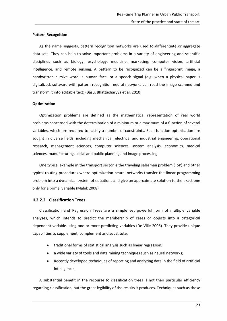
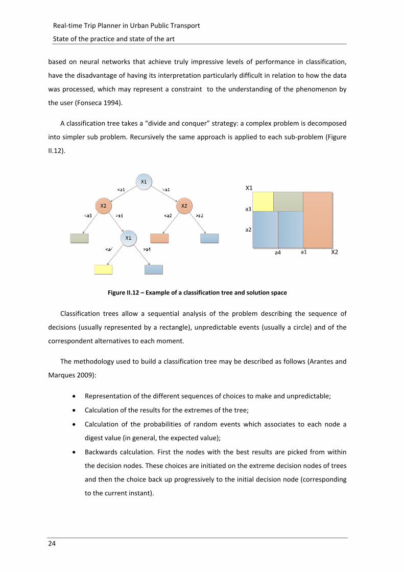
A classification tree takes a “divide and conquer” strategy: a complex problem is decomposed

into simpler sub problem. Recursively the same approach is applied to each sub‐problem (Figure

II.12).

X1

a1

a2

a4 X2

a3

Figure II.12 – Example of a classification tree and solution space

Classification trees allow a sequential analysis of the problem describing the sequence of

decisions (usually represented by a rectangle), unpredictable events (usually a circle) and of the

correspondent alternatives to each moment.

The methodology used to build a classification tree may be described as follows (Arantes and

Marques 2009):

Representation of the different sequences of choices to make and unpredictable;

Calculation of the results for the extremes of the tree;

Calculation of the probabilities of random events which associates to each node a

digest value (in general, the expected value);

Backwards calculation. First the nodes with the best results are picked from within

the decision nodes. These choices are initiated on the extreme decision nodes of trees

and then the choice back up progressively to the initial decision node (corresponding

to the current instant).

25



Recent models based in classification trees are already applied to short‐time traffic prediction

with results achieved of 92.1 % of accuracy on prediction congestion conditions in 30 minutes

advance (Klakhaeng, Yaothanee et al. 2011).

II.2.2.3 Bayesian Statistical Inference

Bayesian inference is a statistical method in which observed evidences are used to update the

uncertainty of probability models. The term "Bayesian" comes from the use of the Bayesian

interpretation of probability. Bayesian inference is often used to make predictions about the

value of model parameters and unknown variables (Smith 2010).

Under the Bayesian interpretation of probability, it measures confidence that something is

true. As events are generated by a process, these may be compared to possible models for the

process. Intuitively, the uncertainty of individual models should tend to 1 or 0 as evidence

accumulates. In Bayesian inference, the necessary adjustment of uncertainty to account for

evidence is calculated using Bayes' theorem. The uncertainty is repeatedly adjusted as fresh

evidence is observed. At each step, the initial uncertainty is called the prior, while the modified

uncertainty is called the posterior (Smith 2010).

Bayesian inference techniques have been a fundamental part of computerized pattern

recognition techniques since the late 1950s. There is also a growing connection between Bayesian

methods and simulation‐based Monte Carlo techniques since complex models cannot be

processed in closed form by a Bayesian analysis, while a graphical model structure may allow for

efficient simulation algorithms like the Gibbs sampling and other Metropolis–Hastings algorithm

schemes (Smith 2010).

Bayesian Statistical Inference procedures have been recently used in the literature also to

predict travel times and speed in road traffic, based on historical statistical distributions.

Normally, these procedures have been encompassed in neural networks formulation, where

input parameters are not direct measures from the network, but inferred statistical distributions

(Park and Lee 2004).

Another approach has been introducing smoothing splines in AVL systems that identify

vehicles detected as discrete points in the traffic network, and sections defined as the length of

the roadway between adjacent detection points. The set of contiguous sections forms a corridor.

The section travel time for a given instrumented vehicle is calculated based on the times at which

each of these vehicles passes a detection point (Gajewski and Rilett 2005).

26



Using these observations, section summary statistics, such as travel time mean and variance

as a function of time of day, can be obtained. The travel time statistics for the corridor may be

obtained directly or be based on the sum of the individual section travel times. In the latter case,

a covariance matrix often is required, because link travel times are rarely independent.

Bayesian statistical inference has the ability to estimate the correlation of section travel

times. In Bayesian inference, the unknown parameters of the probability distributions are

modeled as having distributions of their own (Gelman 2003). Generally, the identification of the

distribution of the parameters, or prior distribution, is done before the data are collected.

Gajewski & Rilett (2005) have demonstrated that their inference method was appropriate,

under several dynamic conditions where the speed range varied between from 8 km/h and 105

km/h, which is in the range of regular traffic conditions.

Bayesian approach has a number of benefits in terms of interpretation and ease of use. Yet, it

requires a significant amount of computational capacity to estimate posterior distributions using

simulation‐based Monte Carlo techniques (Smith 2010).

This approach may present a problem for local disturbances, which might impact slightly

initial in the posterior distribution for a significant number of observations, which would require

the incorporation of a rule‐based approach to identify the presence of this type of phenomena.

II.2.3 Summary and Conclusions

In this chapter were studied some methods used in pattern recognition, data series prediction

and optimization problems. Since we are dealing with valuable information with high commercial

value, companies do not inform how websites and applications compute forecasts nor about the

methodologies behind those predictions. Neural networks, decision trees and Bayesian inference

were selected due to their consideration as potential methodologies to estimate arrival times of

buses and even travel time predictions.

While there are already applications using neural networks, classification trees models or

Bayesian inference methods in traffic forecast systems, they are mainly applied to the road sector

in which only circulation speed disturbances are taken into consideration. These algorithms alone

do not provide solutions to public transport systems that need to manage vehicles dispatch in

order to avoid schedule delays and bus bunching. These characteristics of public transports

27



increase the complexity of the problems due to the interdependence that exists among the

network road sections.

To include the above mentioned public transport constraints in the model to be developed, it

was considered the necessity of integration in the prediction system, algorithms that predict

beyond replicating previously observed patterns, but also incorporate intelligence to change the

system’s behavior to “new” or uncertain operational conditions.

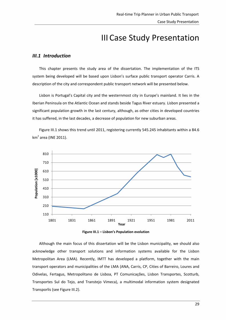
29


Case Study Presentation

III Case Study Presentation

III.1 Introduction

This chapter presents the study area of the dissertation. The implementation of the ITS

system being developed will be based upon Lisbon’s surface public transport operator Carris. A

description of the city and correspondent public transport network will be presented below.

Lisbon is Portugal’s Capital city and the westernmost city in Europe’s mainland. It lies in the

Iberian Peninsula on the Atlantic Ocean and stands beside Tagus River estuary. Lisbon presented a

significant population growth in the last century, although, as other cities in developed countries

it has suffered, in the last decades, a decrease of population for new suburban areas.

Figure III.1 shows this trend until 2011, registering currently 545.245 inhabitants within a 84.6

km2 area (INE 2011).

Figure III.1 – Lisbon’s Population evolution

Although the main focus of this dissertation will be the Lisbon municipality, we should also

acknowledge other transport solutions and information systems available for the Lisbon

Metropolitan Area (LMA). Recently, IMTT has developed a platform, together with the main

transport operators and municipalities of the LMA (ANA, Carris, CP, Cities of Barreiro, Loures and

Odivelas, Fertagus, Metropolitano de Lisboa, PT Comunicações, Lisbon Transportes, Scotturb,

Transportes Sul do Tejo, and Transtejo Vimeca), a multimodal information system designated

Transporlis (see Figure III.2).

110

210

310

410

510

610

710

810

1801 1831 1861 1891 1921 1951 1981 2011

Population [x1000]

Year

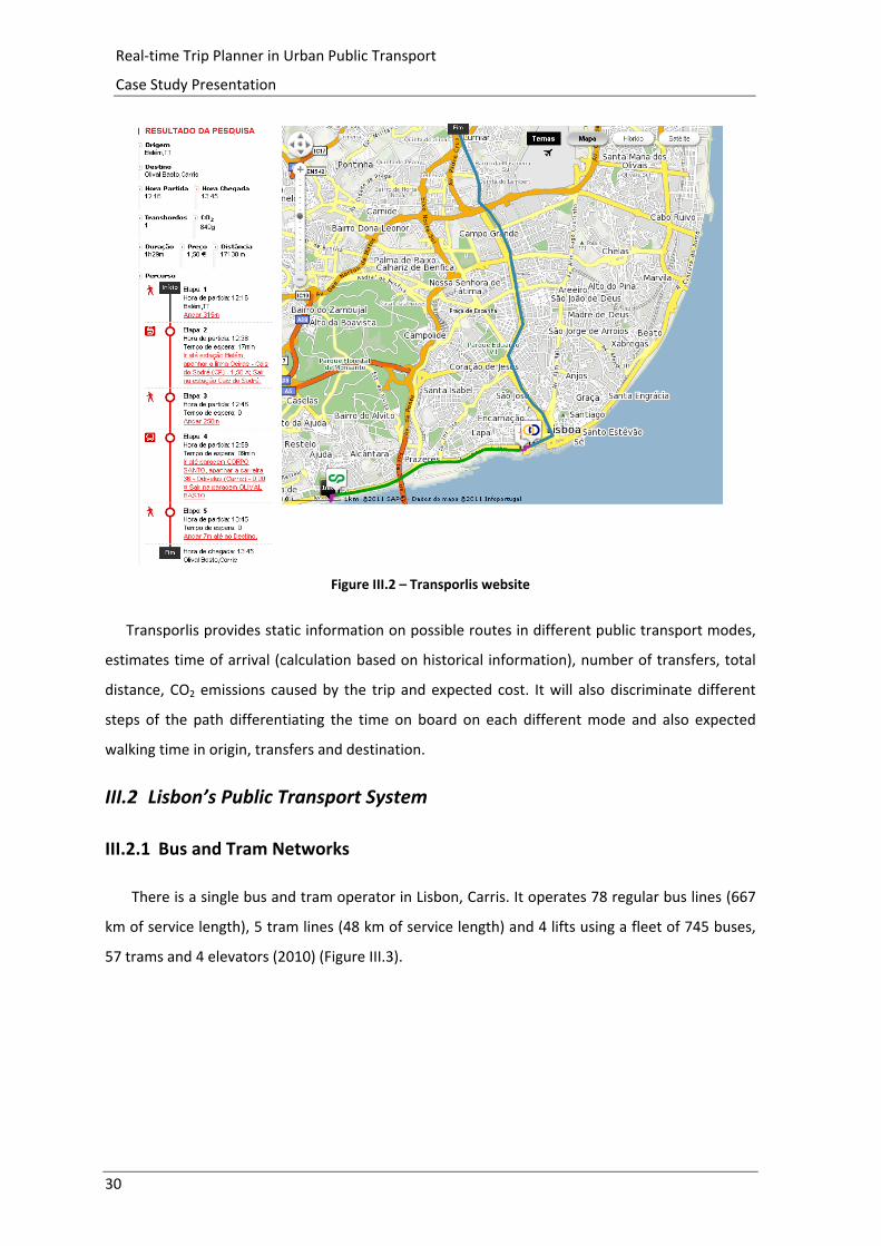
30



Figure III.2 – Transporlis website

Transporlis provides static information on possible routes in different public transport modes,

estimates time of arrival (calculation based on historical information), number of transfers, total

distance, CO2 emissions caused by the trip and expected cost. It will also discriminate different

steps of the path differentiating the time on board on each different mode and also expected

walking time in origin, transfers and destination.

III.2 Lisbon’s Public Transport System

III.2.1 Bus and Tram Networks

There is a single bus and tram operator in Lisbon, Carris. It operates 78 regular bus lines (667

km of service length), 5 tram lines (48 km of service length) and 4 lifts using a fleet of 745 buses,

57 trams and 4 elevators (2010) (Figure III.3).

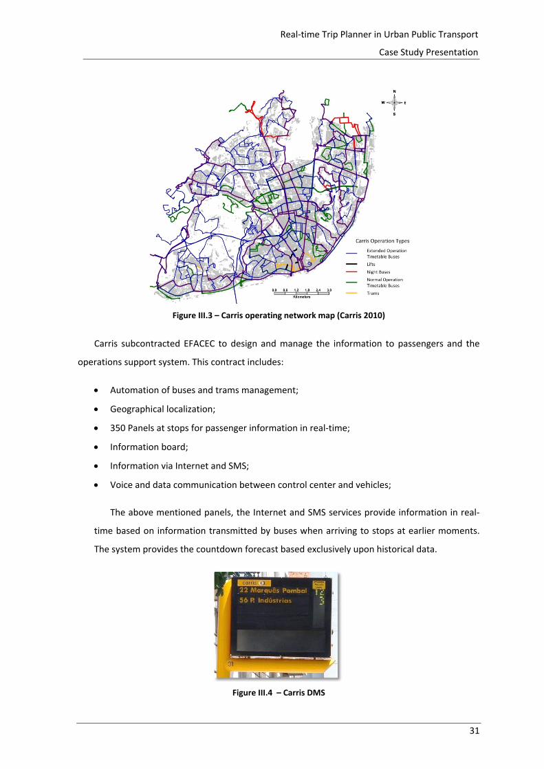
31



Figure III.3 – Carris operating network map (Carris 2010)

Carris subcontracted EFACEC to design and manage the information to passengers and the

operations support system. This contract includes:

Automation of buses and trams management;

Geographical localization;

350 Panels at stops for passenger information in real‐time;

Information board;

Information via Internet and SMS;

Voice and data communication between control center and vehicles;

The above mentioned panels, the Internet and SMS services provide information in real‐

time based on information transmitted by buses when arriving to stops at earlier moments.

The system provides the countdown forecast based exclusively upon historical data.

Figure III.4 – Carris DMS

32



By analyzing Figure I.1 becomes clear that the demand for Carris transport services has seen a

decline in recent years especially since 1986, when Portugal joined the European Union (EU). The

tendency to decrease after this date can be explained by the fact that average incomes of

households have significantly increased leading to an increase in car ownership and suburban

relocation of dwellings (Kenworthy, Laube et al. 1999).

Bus and tram stops are a key element of the mobility system design. Yet, their location might

produce significant impacts on traffic circulation by interrupting flows while buses and trams

approach and stop. In urban traffic systems, there are often multi bus stops on a road, so the

distance between bus stops will have great effects on traffic flow and produce some complex

traffic phenomena (Tang 2010). For that reason, it was performed a short analysis evaluating the

distance between stops in Carris roadway.

The statistical distribution of distances between consecutive stops of the same line (shown

with cumulative probability and probability density functions) is as shown in Figure III.5.

Figure III.5 – Distance between stops analysis

To this analysis only sections between stops used by a Carris bus line were considered. The

data set was constituted by 4805 sections, and the analysis produced an average distance

between stops of 369.8 m with a standard deviation of 274.1 m. The median value computed was

322.5 m. While it is important to notice the need for longer sections when in the presence of

overlaps with highways it should be also acknowledged that short sections must be avoided if

commercial speed is important (except on high slope roads that would impose a bit access effort

to clients).

0

0,0002

0,0004

0,0006

0,0008

0,001

0,0012

0,0014

0,0016

0

0,2

0,4

0,6

0,8

1

0 200 400 600 800 1000

Probab

ility Density

Cumulative probab

ility

Distance between stops [m]Cummulative probability Adjusted Normal Distribution

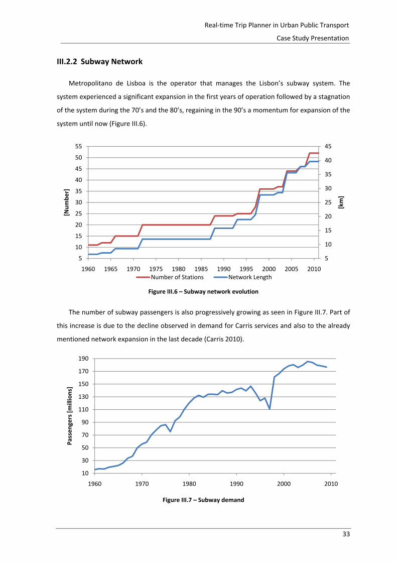
33



III.2.2 Subway Network

Metropolitano de Lisboa is the operator that manages the Lisbon’s subway system. The

system experienced a significant expansion in the first years of operation followed by a stagnation

of the system during the 70’s and the 80’s, regaining in the 90’s a momentum for expansion of the

system until now (Figure III.6).

Figure III.6 – Subway network evolution

The number of subway passengers is also progressively growing as seen in Figure III.7. Part of

this increase is due to the decline observed in demand for Carris services and also to the already

mentioned network expansion in the last decade (Carris 2010).

Figure III.7 – Subway demand

5

10

15

20

25

30

35

40

45

5

10

15

20

25

30

35

40

45

50

55

1960 1965 1970 1975 1980 1985 1990 1995 2000 2005 2010

[km]

[Number]

Number of Stations Network Length

10

30

50

70

90

110

130

150

170

190

1960 1970 1980 1990 2000 2010

Passengers [millions]

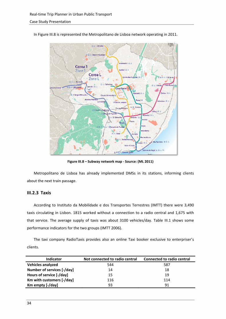
34



In Figure III.8 is represented the Metropolitano de Lisboa network operating in 2011.

Figure III.8 – Subway network map ‐ Source: (ML 2011)

Metropolitano de Lisboa has already implemented DMSs in its stations, informing clients

about the next train passage.

III.2.3 Taxis

According to Instituto da Mobilidade e dos Transportes Terrestres (IMTT) there were 3,490

taxis circulating in Lisbon. 1815 worked without a connection to a radio central and 1,675 with

that service. The average supply of taxis was about 3100 vehicles/day. Table III.1 shows some

performance indicators for the two groups (IMTT 2006).

The taxi company RadioTaxis provides also an online Taxi booker exclusive to enterpriser’s

clients.

Indicator Not connected to radio central Connected to radio central

Vehicles analyzed 544 587 Number of services [‐/day] 14 18 Hours of service [‐/day] 15 19 Km with customers [‐/day] 116 114 Km empty [‐/day] 93 91

35



Indicator Not connected to radio central Connected to radio central

[Km/day] 209 205 Revenue [€/year] 26,598 31302 Costs [€/year] 25763 28660 Profit [€/year] 835 2642

Table III.1 – Operating indicators comparison: 365 days working taxi

The indicators express that a taxi with a communication system to a central is on average

three times more profitable than the non‐connected taxi.

III.3 Conclusions

Some effort has been put in introducing information aiding systems for customers in public

transport. Yet, their large scale implementation and the introduction of more high‐tech solutions

are still to be deployed.

Although this study will focus only on the Carris network inside Lisbon, there is the

potentiality to integrate in the future other transport modes, presented above, which also may

take advantage of this system, and also promote a better integration an level of service on the

overall public transport system.

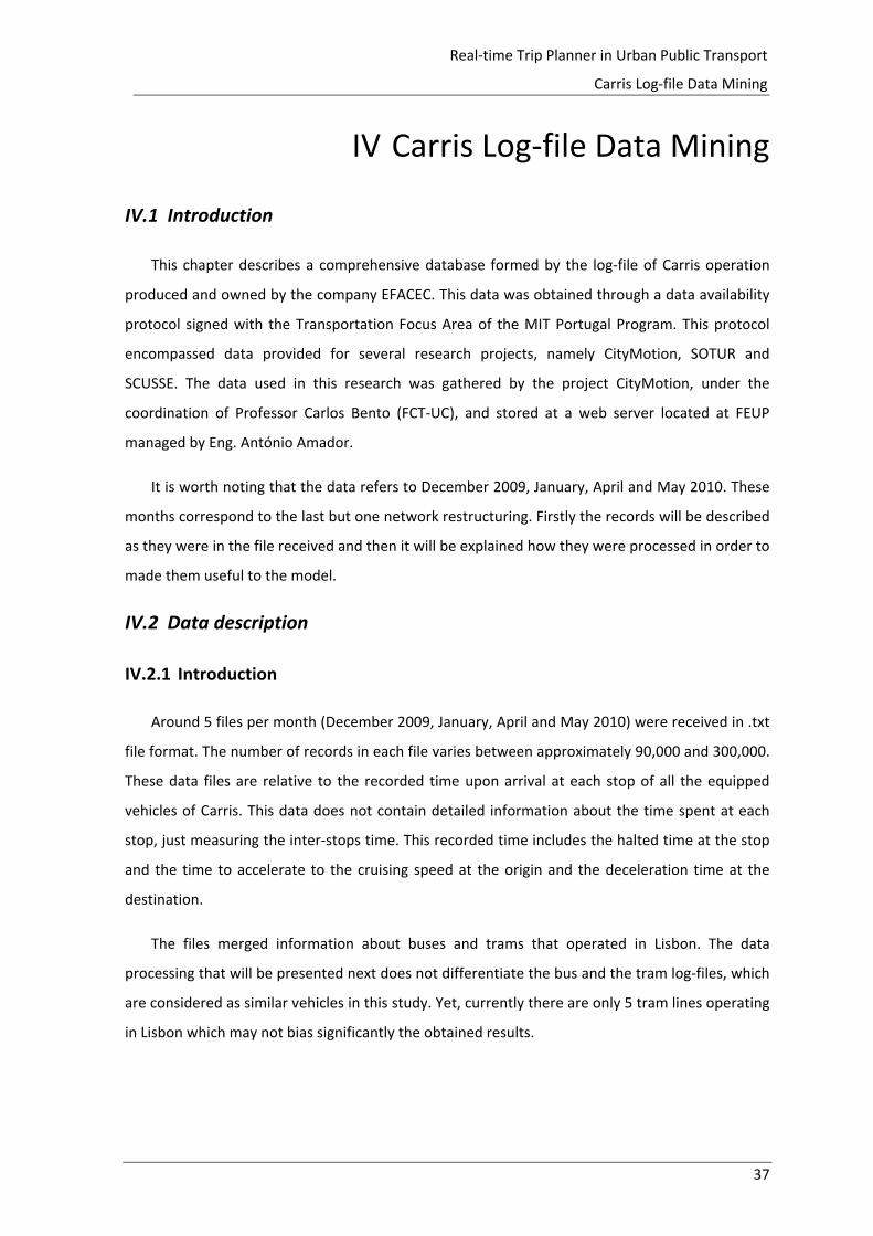
37


Carris Log‐file Data Mining

IV Carris Log‐file Data Mining

IV.1 Introduction

This chapter describes a comprehensive database formed by the log‐file of Carris operation

produced and owned by the company EFACEC. This data was obtained through a data availability

protocol signed with the Transportation Focus Area of the MIT Portugal Program. This protocol

encompassed data provided for several research projects, namely CityMotion, SOTUR and

SCUSSE. The data used in this research was gathered by the project CityMotion, under the

coordination of Professor Carlos Bento (FCT‐UC), and stored at a web server located at FEUP

managed by Eng. António Amador.

It is worth noting that the data refers to December 2009, January, April and May 2010. These

months correspond to the last but one network restructuring. Firstly the records will be described

as they were in the file received and then it will be explained how they were processed in order to

made them useful to the model.

IV.2 Data description

IV.2.1 Introduction

Around 5 files per month (December 2009, January, April and May 2010) were received in .txt

file format. The number of records in each file varies between approximately 90,000 and 300,000.

These data files are relative to the recorded time upon arrival at each stop of all the equipped

vehicles of Carris. This data does not contain detailed information about the time spent at each

stop, just measuring the inter‐stops time. This recorded time includes the halted time at the stop

and the time to accelerate to the cruising speed at the origin and the deceleration time at the

destination.

The files merged information about buses and trams that operated in Lisbon. The data

processing that will be presented next does not differentiate the bus and the tram log‐files, which

are considered as similar vehicles in this study. Yet, currently there are only 5 tram lines operating

in Lisbon which may not bias significantly the obtained results.

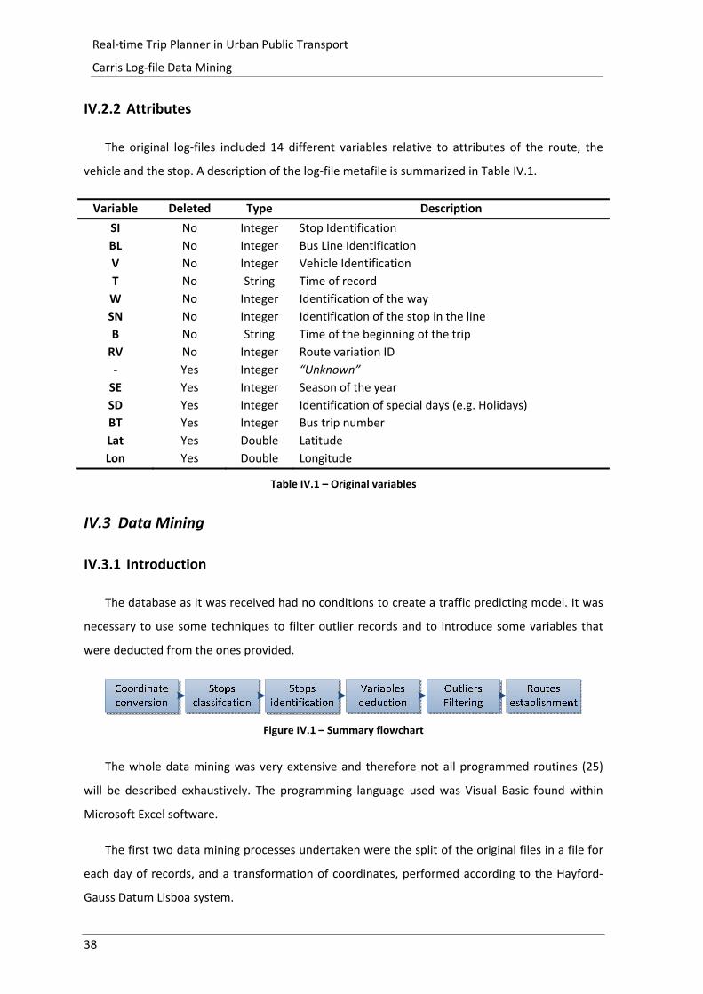
38



IV.2.2 Attributes

The original log‐files included 14 different variables relative to attributes of the route, the

vehicle and the stop. A description of the log‐file metafile is summarized in Table IV.1.

Variable Deleted Type Description

SI No Integer Stop Identification

BL No Integer Bus Line Identification

V No Integer Vehicle Identification

T No String Time of record

W No Integer Identification of the way

SN No Integer Identification of the stop in the line

B No String Time of the beginning of the trip

RV No Integer Route variation ID

‐ Yes Integer “Unknown”

SE Yes Integer Season of the year

SD Yes Integer Identification of special days (e.g. Holidays)

BT Yes Integer Bus trip number

Lat Yes Double Latitude

Lon Yes Double Longitude

Table IV.1 – Original variables

IV.3 Data Mining

IV.3.1 Introduction

The database as it was received had no conditions to create a traffic predicting model. It was

necessary to use some techniques to filter outlier records and to introduce some variables that

were deducted from the ones provided.

Figure IV.1 – Summary flowchart

The whole data mining was very extensive and therefore not all programmed routines (25)

will be described exhaustively. The programming language used was Visual Basic found within

Microsoft Excel software.

The first two data mining processes undertaken were the split of the original files in a file for

each day of records, and a transformation of coordinates, performed according to the Hayford‐

Gauss Datum Lisboa system.

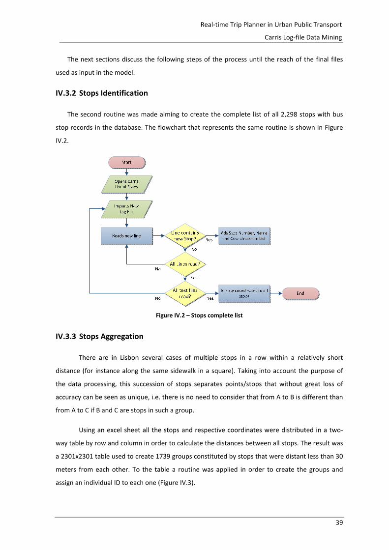
39



The next sections discuss the following steps of the process until the reach of the final files

used as input in the model.

IV.3.2 Stops Identification

The second routine was made aiming to create the complete list of all 2,298 stops with bus

stop records in the database. The flowchart that represents the same routine is shown in Figure

IV.2.

Figure IV.2 – Stops complete list

IV.3.3 Stops Aggregation

There are in Lisbon several cases of multiple stops in a row within a relatively short

distance (for instance along the same sidewalk in a square). Taking into account the purpose of

the data processing, this succession of stops separates points/stops that without great loss of

accuracy can be seen as unique, i.e. there is no need to consider that from A to B is different than

from A to C if B and C are stops in such a group.

Using an excel sheet all the stops and respective coordinates were distributed in a two‐

way table by row and column in order to calculate the distances between all stops. The result was

a 2301x2301 table used to create 1739 groups constituted by stops that were distant less than 30

meters from each other. To the table a routine was applied in order to create the groups and

assign an individual ID to each one (Figure IV.3).

40



Figure IV.3 – Group creation

After the creation of the groups it was necessary to calculate the geometrical centroid of

each group. For that purpose, it was used an Excel pivot table that calculated the average of X and

Y coordinates of the stops that constituted every group which created variables X_O, Y_O, X_D

and Y_ D.

IV.3.4 Variables Deduction

A routine was then created to complete the files with missing information according to the

flowchart in Figure IV.4.

Figure IV.4 – New variable computation

Start

Opens file

Reads new line

Finds all Stops closer than 30m to Stop on line

NoAll lines read?

Yes Completes each line with remain Stop closer than

30m

Deletes lines with the same stops

Assigns an individual number to each group

End

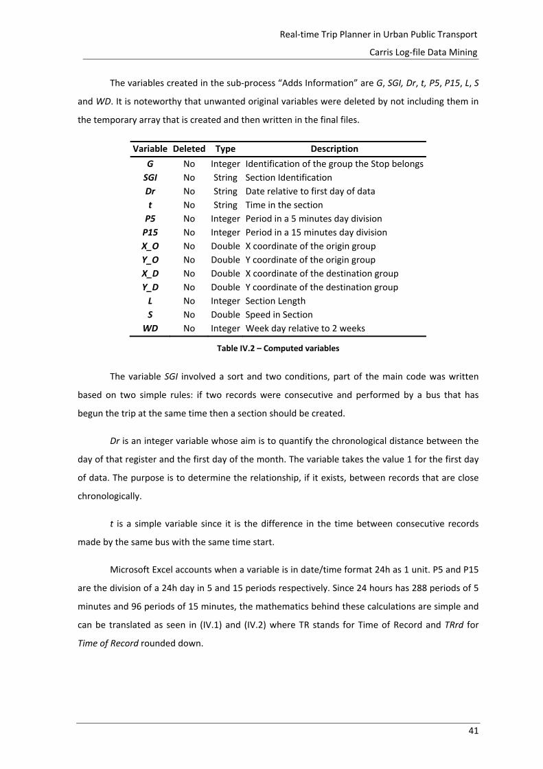
41



The variables created in the sub‐process “Adds Information” are G, SGI, Dr, t, P5, P15, L, S

and WD. It is noteworthy that unwanted original variables were deleted by not including them in

the temporary array that is created and then written in the final files.

Variable Deleted Type Description

G No Integer Identification of the group the Stop belongs

SGI No String Section Identification

Dr No String Date relative to first day of data

t No String Time in the section

P5 No Integer Period in a 5 minutes day division

P15 No Integer Period in a 15 minutes day division

X_O No Double X coordinate of the origin group

Y_O No Double Y coordinate of the origin group

X_D No Double X coordinate of the destination group

Y_D No Double Y coordinate of the destination group

L No Integer Section Length

S No Double Speed in Section

WD No Integer Week day relative to 2 weeks

Table IV.2 – Computed variables

The variable SGI involved a sort and two conditions, part of the main code was written

based on two simple rules: if two records were consecutive and performed by a bus that has

begun the trip at the same time then a section should be created.

Dr is an integer variable whose aim is to quantify the chronological distance between the

day of that register and the first day of the month. The variable takes the value 1 for the first day

of data. The purpose is to determine the relationship, if it exists, between records that are close

chronologically.

t is a simple variable since it is the difference in the time between consecutive records

made by the same bus with the same time start.

Microsoft Excel accounts when a variable is in date/time format 24h as 1 unit. P5 and P15

are the division of a 24h day in 5 and 15 periods respectively. Since 24 hours has 288 periods of 5

minutes and 96 periods of 15 minutes, the mathematics behind these calculations are simple and

can be translated as seen in (IV.1) and (IV.2) where TR stands for Time of Record and TRrd for

Time of Record rounded down.

42



5 1288

(IV.1)

15 196

(IV.2)

It is important to notice that at this stage of the study the length of each road section is

the smallest distance between stops in the extremities of the section. L is the Euclidean Distance

between different group centroid coordinates.

The speed in each section was calculated according to / where S stands for Speed,

d for distance and t for time. As the used distance to compute this variable is the Euclidean

distance between stops, the obtained speed represents the equivalent speed that would results

from a direct connection instead of following the paths within the road network.

WD is similar to DRr with the exception that refers to week days (Monday, Tuesday, etc.)

and not month days (1, 2, 3, etc.) in a 2 week cycle. Although both variables have been computed,

it was considered that the data sample was not big enough in terms of different record days for a

relationship creation between days.

IV.3.5 Outlier Filtering

The processed files revealed that some sections were traveled by buses an insufficient

number of times for them to belong to usual bus lines. It was deduced that these sections

correspond to sporadic service interruptions, breakdowns or other incidents. In order to eliminate

these outliers that were considered insignificant for the traffic prediction model to be constructed

a routine was created to eliminate records containing sections that appeared in all records less

than 10 times.

IV.3.6 Route Establishment

Not all vehicles travel through scheduled routes all the time. There are occasional incidents or

accidents that prevent the normal course of buses. A routine was created to determine routes

that each bus has effectively traversed and how many times each one was traveled according to

Figure IV.5.

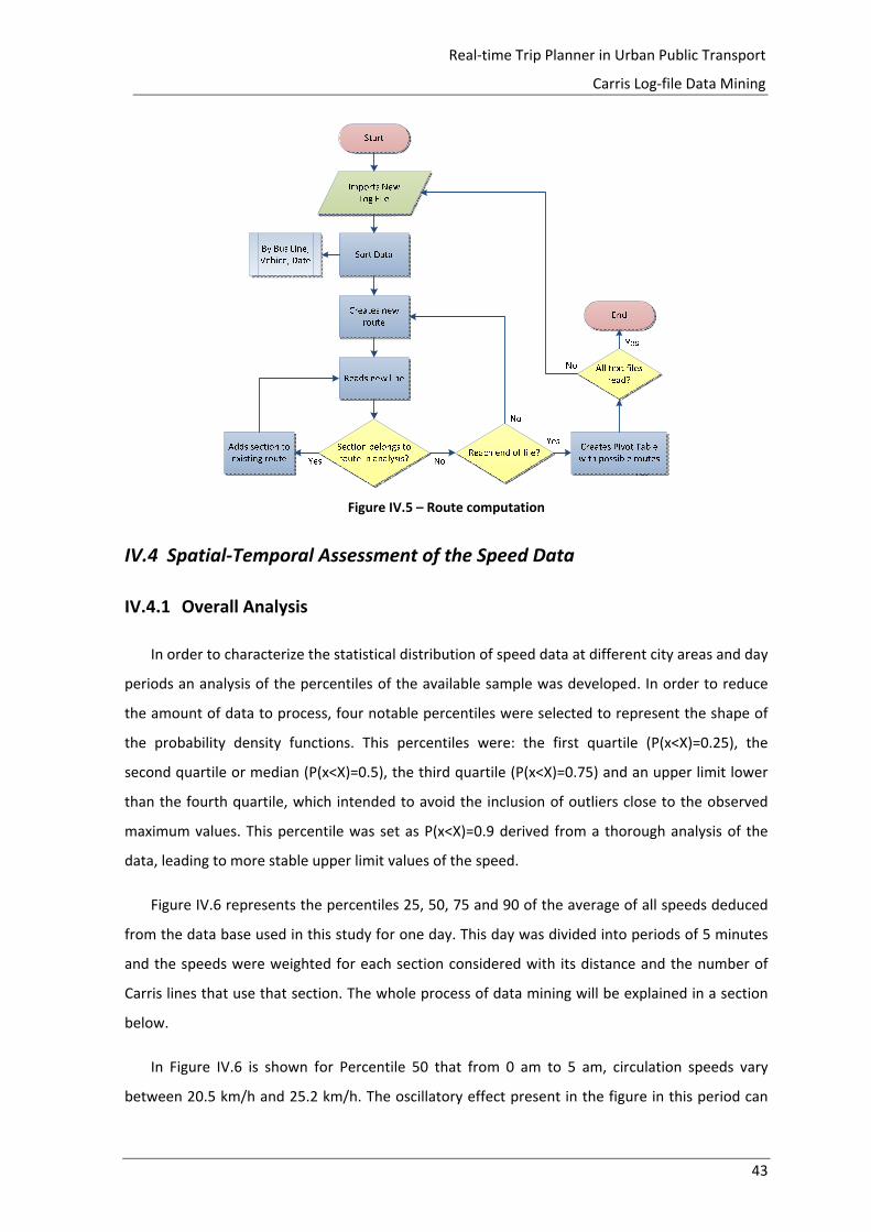
43



Figure IV.5 – Route computation

IV.4 Spatial‐Temporal Assessment of the Speed Data

IV.4.1 Overall Analysis

In order to characterize the statistical distribution of speed data at different city areas and day

periods an analysis of the percentiles of the available sample was developed. In order to reduce

the amount of data to process, four notable percentiles were selected to represent the shape of

the probability density functions. This percentiles were: the first quartile (P(x<X)=0.25), the

second quartile or median (P(x<X)=0.5), the third quartile (P(x<X)=0.75) and an upper limit lower

than the fourth quartile, which intended to avoid the inclusion of outliers close to the observed

maximum values. This percentile was set as P(x<X)=0.9 derived from a thorough analysis of the

data, leading to more stable upper limit values of the speed.

Figure IV.6 represents the percentiles 25, 50, 75 and 90 of the average of all speeds deduced

from the data base used in this study for one day. This day was divided into periods of 5 minutes

and the speeds were weighted for each section considered with its distance and the number of

Carris lines that use that section. The whole process of data mining will be explained in a section

below.

In Figure IV.6 is shown for Percentile 50 that from 0 am to 5 am, circulation speeds vary

between 20.5 km/h and 25.2 km/h. The oscillatory effect present in the figure in this period can

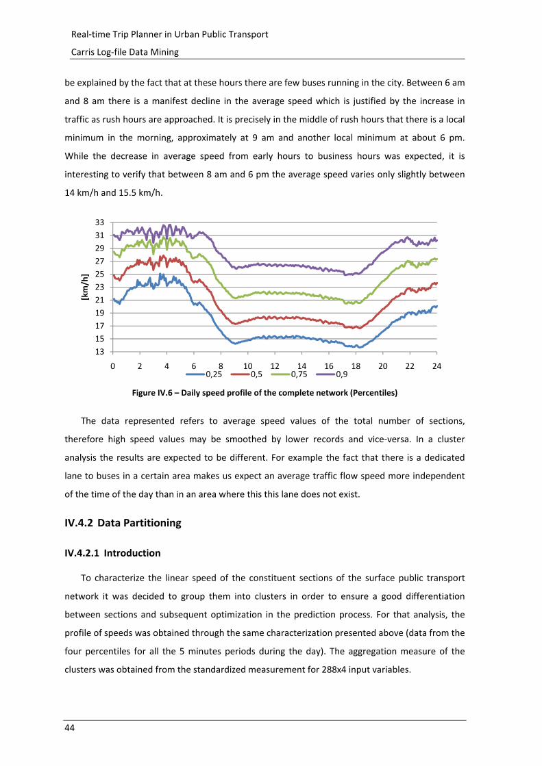
44



be explained by the fact that at these hours there are few buses running in the city. Between 6 am

and 8 am there is a manifest decline in the average speed which is justified by the increase in

traffic as rush hours are approached. It is precisely in the middle of rush hours that there is a local

minimum in the morning, approximately at 9 am and another local minimum at about 6 pm.

While the decrease in average speed from early hours to business hours was expected, it is

interesting to verify that between 8 am and 6 pm the average speed varies only slightly between

14 km/h and 15.5 km/h.

Figure IV.6 – Daily speed profile of the complete network (Percentiles)

The data represented refers to average speed values of the total number of sections,

therefore high speed values may be smoothed by lower records and vice‐versa. In a cluster

analysis the results are expected to be different. For example the fact that there is a dedicated

lane to buses in a certain area makes us expect an average traffic flow speed more independent

of the time of the day than in an area where this this lane does not exist.

IV.4.2 Data Partitioning

IV.4.2.1 Introduction

To characterize the linear speed of the constituent sections of the surface public transport

network it was decided to group them into clusters in order to ensure a good differentiation

between sections and subsequent optimization in the prediction process. For that analysis, the

profile of speeds was obtained through the same characterization presented above (data from the

four percentiles for all the 5 minutes periods during the day). The aggregation measure of the

clusters was obtained from the standardized measurement for 288x4 input variables.

13

15

17

19

21

23

25

27

29

31

33

0 2 4 6 8 10 12 14 16 18 20 22 24

[km/h]

0,25 0,5 0,75 0,9

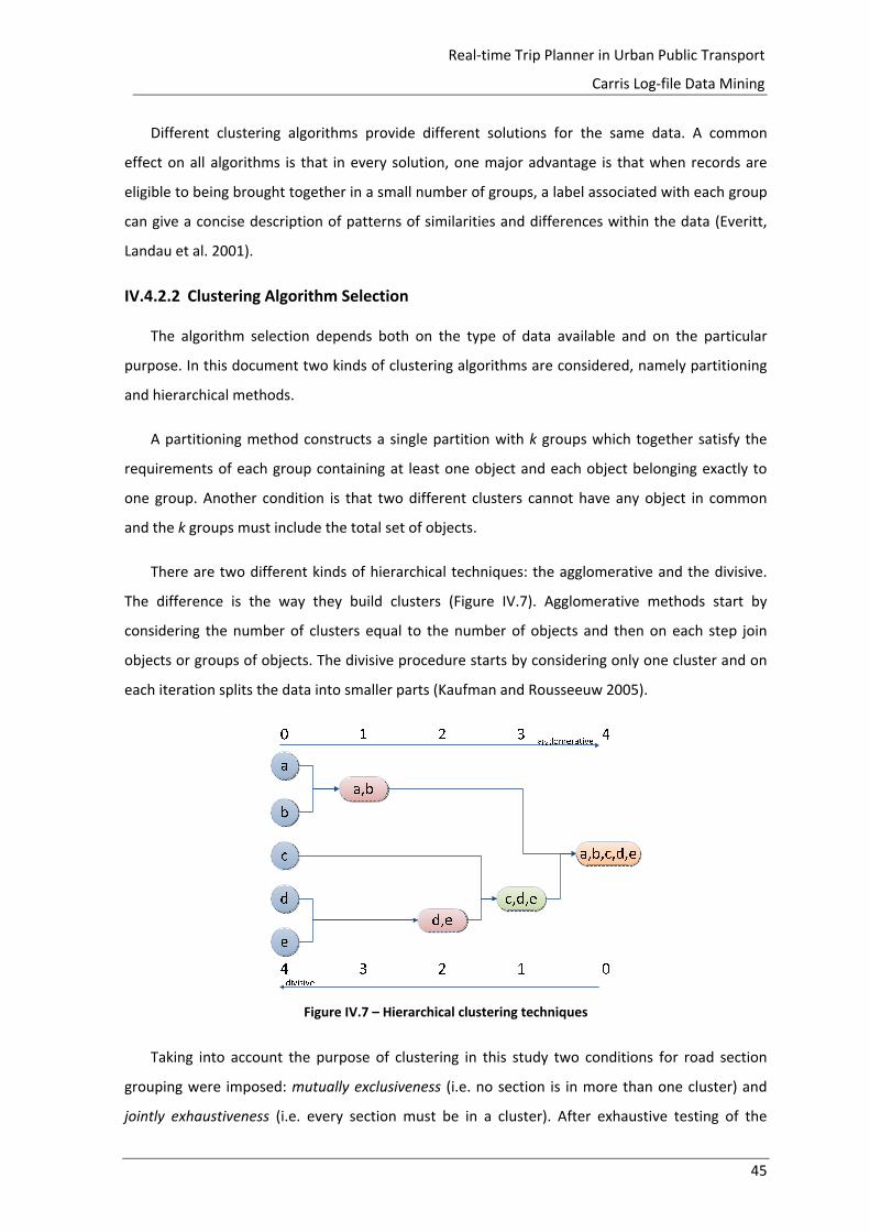
45



Different clustering algorithms provide different solutions for the same data. A common

effect on all algorithms is that in every solution, one major advantage is that when records are

eligible to being brought together in a small number of groups, a label associated with each group

can give a concise description of patterns of similarities and differences within the data (Everitt,

Landau et al. 2001).

IV.4.2.2 Clustering Algorithm Selection

The algorithm selection depends both on the type of data available and on the particular

purpose. In this document two kinds of clustering algorithms are considered, namely partitioning

and hierarchical methods.

A partitioning method constructs a single partition with k groups which together satisfy the

requirements of each group containing at least one object and each object belonging exactly to

one group. Another condition is that two different clusters cannot have any object in common

and the k groups must include the total set of objects.

There are two different kinds of hierarchical techniques: the agglomerative and the divisive.

The difference is the way they build clusters (Figure IV.7). Agglomerative methods start by

considering the number of clusters equal to the number of objects and then on each step join

objects or groups of objects. The divisive procedure starts by considering only one cluster and on

each iteration splits the data into smaller parts (Kaufman and Rousseeuw 2005).

Figure IV.7 – Hierarchical clustering techniques

Taking into account the purpose of clustering in this study two conditions for road section

grouping were imposed: mutually exclusiveness (i.e. no section is in more than one cluster) and

jointly exhaustiveness (i.e. every section must be in a cluster). After exhaustive testing of the

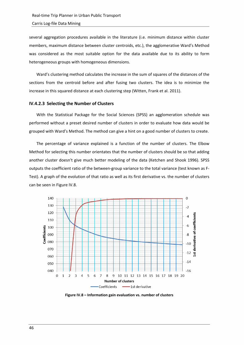
46



several aggregation procedures available in the literature (i.e. minimum distance within cluster

members, maximum distance between cluster centroids, etc.), the agglomerative Ward’s Method

was considered as the most suitable option for the data available due to its ability to form

heterogeneous groups with homogeneous dimensions.

Ward’s clustering method calculates the increase in the sum of squares of the distances of the

sections from the centroid before and after fusing two clusters. The idea is to minimize the

increase in this squared distance at each clustering step (Witten, Frank et al. 2011).

IV.4.2.3 Selecting the Number of Clusters

With the Statistical Package for the Social Sciences (SPSS) an agglomeration schedule was

performed without a preset desired number of clusters in order to evaluate how data would be

grouped with Ward’s Method. The method can give a hint on a good number of clusters to create.

The percentage of variance explained is a function of the number of clusters. The Elbow

Method for selecting this number orientates that the number of clusters should be so that adding

another cluster doesn't give much better modeling of the data (Ketchen and Shook 1996). SPSS

outputs the coefficient ratio of the between‐group variance to the total variance (test known as F‐

Test). A graph of the evolution of that ratio as well as its first derivative vs. the number of clusters

can be seen in Figure IV.8.

Figure IV.8 – Information gain evaluation vs. number of clusters

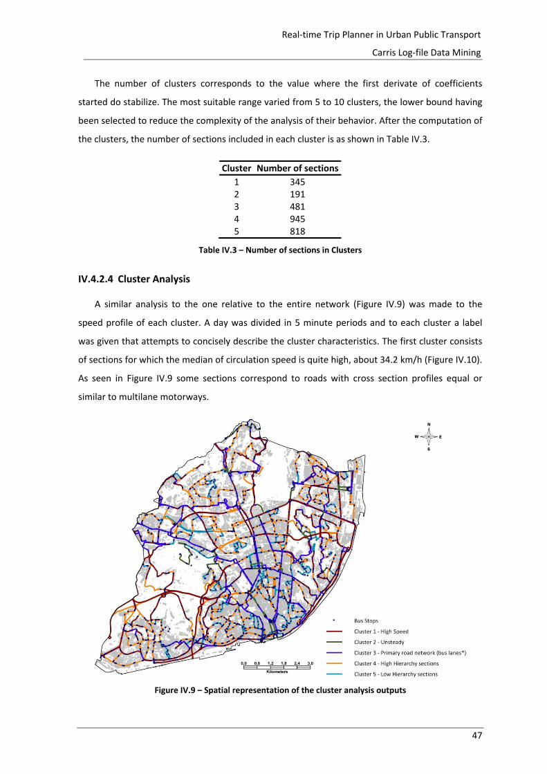
47



The number of clusters corresponds to the value where the first derivate of coefficients

started do stabilize. The most suitable range varied from 5 to 10 clusters, the lower bound having

been selected to reduce the complexity of the analysis of their behavior. After the computation of

the clusters, the number of sections included in each cluster is as shown in Table IV.3.

Cluster Number of sections

1 345 2 191 3 481 4 945 5 818

Table IV.3 – Number of sections in Clusters

IV.4.2.4 Cluster Analysis

A similar analysis to the one relative to the entire network (Figure IV.9) was made to the

speed profile of each cluster. A day was divided in 5 minute periods and to each cluster a label

was given that attempts to concisely describe the cluster characteristics. The first cluster consists

of sections for which the median of circulation speed is quite high, about 34.2 km/h (Figure IV.10).

As seen in Figure IV.9 some sections correspond to roads with cross section profiles equal or

similar to multilane motorways.

Figure IV.9 – Spatial representation of the cluster analysis outputs

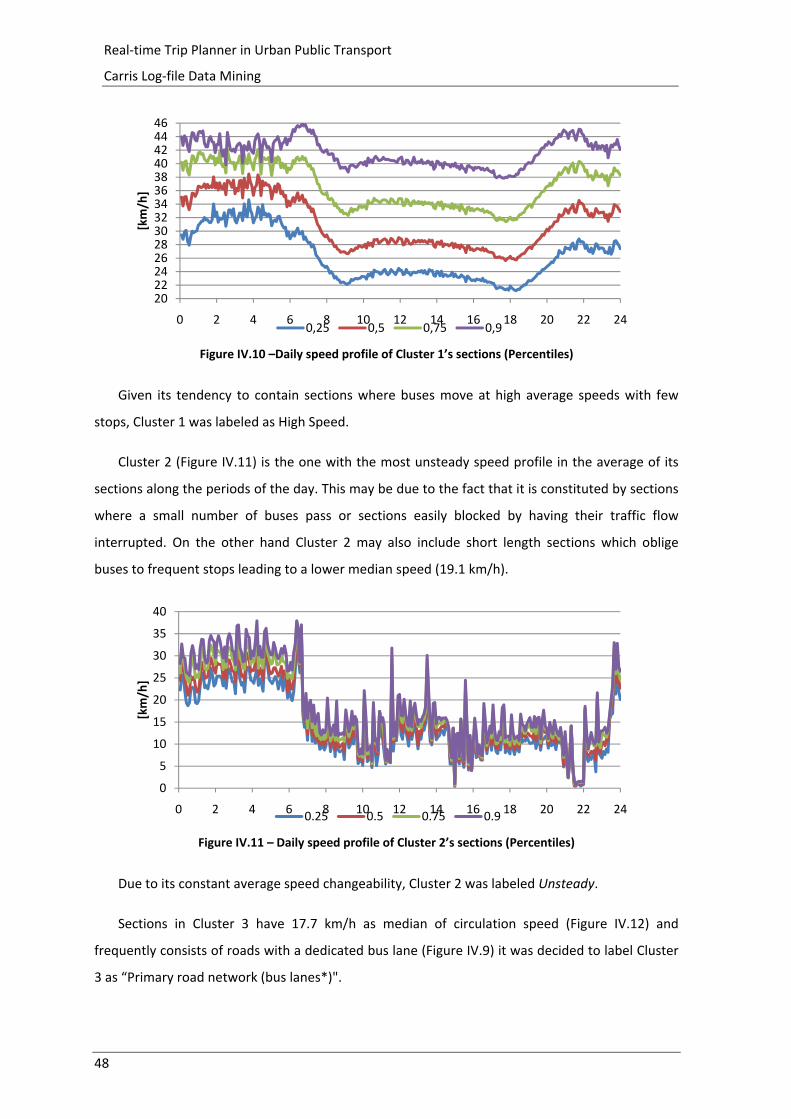
48



Figure IV.10 –Daily speed profile of Cluster 1’s sections (Percentiles)

Given its tendency to contain sections where buses move at high average speeds with few

stops, Cluster 1 was labeled as High Speed.

Cluster 2 (Figure IV.11) is the one with the most unsteady speed profile in the average of its

sections along the periods of the day. This may be due to the fact that it is constituted by sections

where a small number of buses pass or sections easily blocked by having their traffic flow

interrupted. On the other hand Cluster 2 may also include short length sections which oblige

buses to frequent stops leading to a lower median speed (19.1 km/h).

Figure IV.11 – Daily speed profile of Cluster 2’s sections (Percentiles)

Due to its constant average speed changeability, Cluster 2 was labeled Unsteady.

Sections in Cluster 3 have 17.7 km/h as median of circulation speed (Figure IV.12) and

frequently consists of roads with a dedicated bus lane (Figure IV.9) it was decided to label Cluster

3 as “Primary road network (bus lanes*)".

2022242628303234363840424446

0 2 4 6 8 10 12 14 16 18 20 22 24

[km/h]

0,25 0,5 0,75 0,9

0

5

10

15

20

25

30

35

40

0 2 4 6 8 10 12 14 16 18 20 22 24

[km/h]

0.25 0.5 0.75 0.9

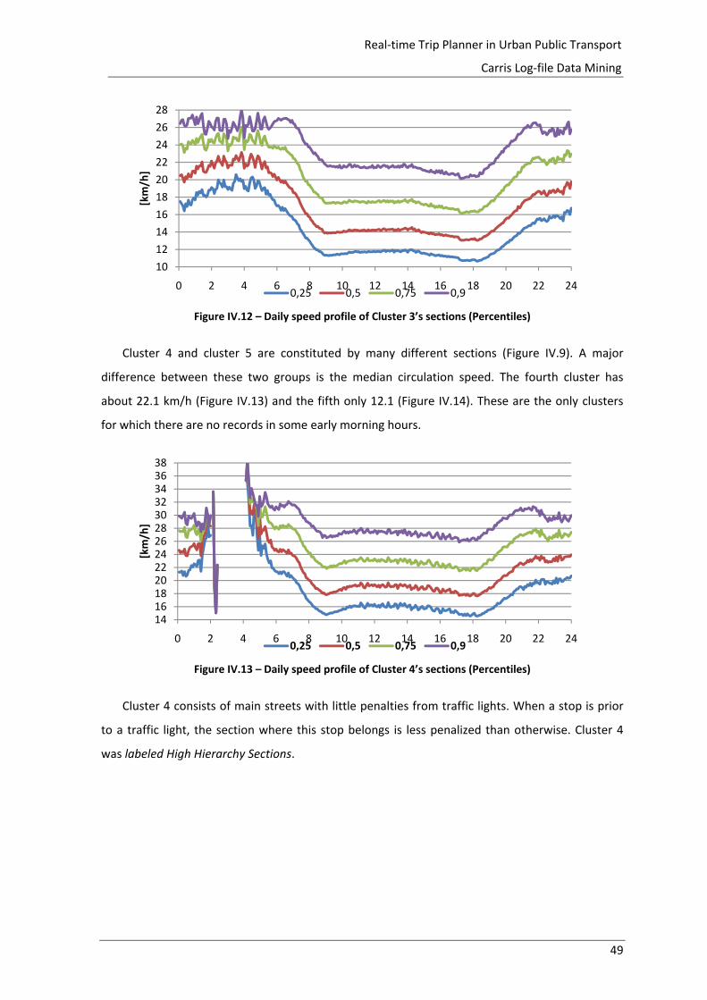
49




Cluster 4 and cluster 5 are constituted by many different sections (Figure IV.9). A major

difference between these two groups is the median circulation speed. The fourth cluster has

about 22.1 km/h (Figure IV.13) and the fifth only 12.1 (Figure IV.14). These are the only clusters

for which there are no records in some early morning hours.


Cluster 4 consists of main streets with little penalties from traffic lights. When a stop is prior

to a traffic light, the section where this stop belongs is less penalized than otherwise. Cluster 4

was labeled High Hierarchy Sections.

10

12

14

16

18

20

22

24

26

28

0 2 4 6 8 10 12 14 16 18 20 22 24

[km/h]

0,25 0,5 0,75 0,9

14161820222426283032343638

0 2 4 6 8 10 12 14 16 18 20 22 24

[km/h]

0,25 0,5 0,75 0,9

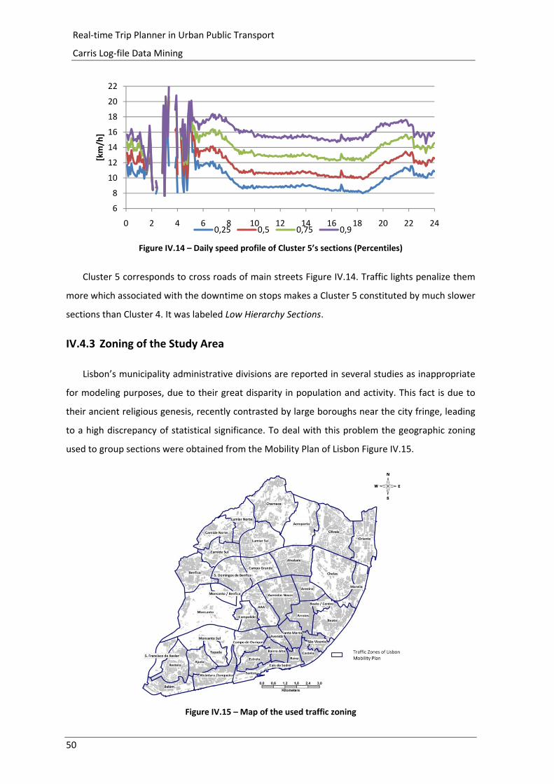
50




Cluster 5 corresponds to cross roads of main streets Figure IV.14. Traffic lights penalize them

more which associated with the downtime on stops makes a Cluster 5 constituted by much slower

sections than Cluster 4. It was labeled Low Hierarchy Sections.

IV.4.3 Zoning of the Study Area

Lisbon’s municipality administrative divisions are reported in several studies as inappropriate

for modeling purposes, due to their great disparity in population and activity. This fact is due to

their ancient religious genesis, recently contrasted by large boroughs near the city fringe, leading

to a high discrepancy of statistical significance. To deal with this problem the geographic zoning

used to group sections were obtained from the Mobility Plan of Lisbon Figure IV.15.

Figure IV.15 – Map of the used traffic zoning

6

8

10

12

14

16

18

20

22

0 2 4 6 8 10 12 14 16 18 20 22 24

[km/h]

0,25 0,5 0,75 0,9

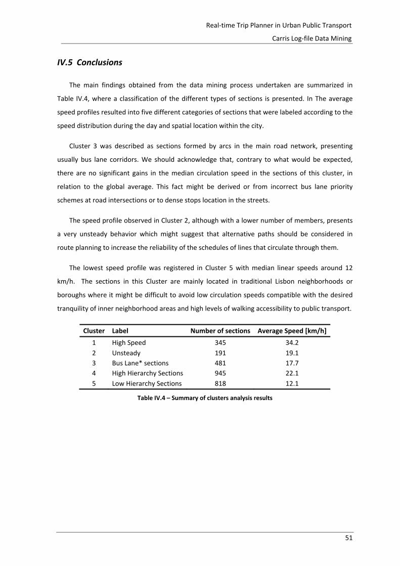
51



IV.5 Conclusions

The main findings obtained from the data mining process undertaken are summarized in

Table IV.4, where a classification of the different types of sections is presented. In The average

speed profiles resulted into five different categories of sections that were labeled according to the

speed distribution during the day and spatial location within the city.

Cluster 3 was described as sections formed by arcs in the main road network, presenting

usually bus lane corridors. We should acknowledge that, contrary to what would be expected,

there are no significant gains in the median circulation speed in the sections of this cluster, in

relation to the global average. This fact might be derived or from incorrect bus lane priority

schemes at road intersections or to dense stops location in the streets.

The speed profile observed in Cluster 2, although with a lower number of members, presents

a very unsteady behavior which might suggest that alternative paths should be considered in

route planning to increase the reliability of the schedules of lines that circulate through them.

The lowest speed profile was registered in Cluster 5 with median linear speeds around 12

km/h. The sections in this Cluster are mainly located in traditional Lisbon neighborhoods or

boroughs where it might be difficult to avoid low circulation speeds compatible with the desired

tranquility of inner neighborhood areas and high levels of walking accessibility to public transport.

Cluster Label Number of sections Average Speed [km/h]

1 High Speed 345 34.2

2 Unsteady 191 19.1

3 Bus Lane* sections 481 17.7

4 High Hierarchy Sections 945 22.1

5 Low Hierarchy Sections 818 12.1

Table IV.4 – Summary of clusters analysis results

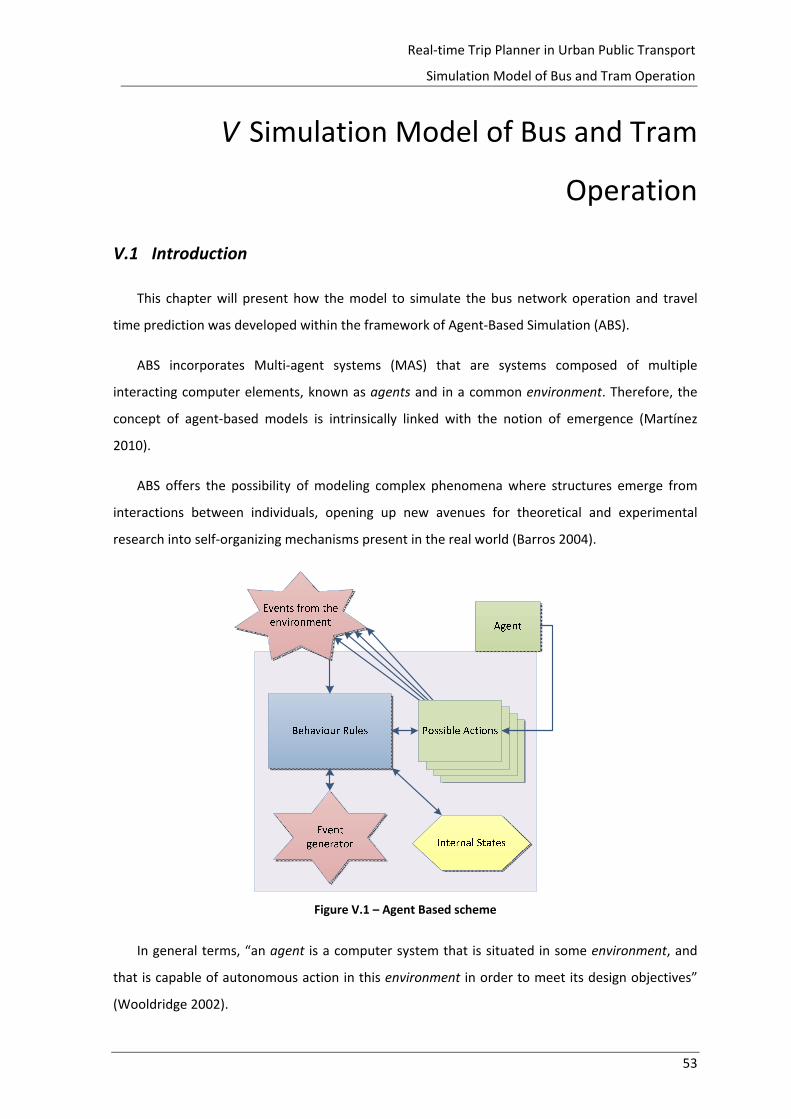
53


Simulation Model of Bus and Tram Operation

V Simulation Model of Bus and Tram

Operation

V.1 Introduction

This chapter will present how the model to simulate the bus network operation and travel

time prediction was developed within the framework of Agent‐Based Simulation (ABS).

ABS incorporates Multi‐agent systems (MAS) that are systems composed of multiple

interacting computer elements, known as agents and in a common environment. Therefore, the

concept of agent‐based models is intrinsically linked with the notion of emergence (Martínez

2010).

ABS offers the possibility of modeling complex phenomena where structures emerge from

interactions between individuals, opening up new avenues for theoretical and experimental

research into self‐organizing mechanisms present in the real world (Barros 2004).

Figure V.1 – Agent Based scheme

In general terms, “an agent is a computer system that is situated in some environment, and

that is capable of autonomous action in this environment in order to meet its design objectives”

(Wooldridge 2002).

54



Multi‐agent simulation (MAS) allows the possibility of directly representing individuals, their

behavior and their interactions (among them and with the environment, see Figure V.1).

The model presented here was written in the JAVA Programming Language, using AnyLogic.

This is a software platform to create agent‐based simulations, system dynamics modeling and

discrete event simulations using the JAVA language developed by a research group in Saint

Petersburg, Russia.

AnyLogic provides a library of JAVA classes for creating, running, displaying and collecting data

from complex simulation environments. In addition, AnyLogic allows the user to customize

simulation outputs.

For the development of this model, two main classes of objects available in AnyLogic libraries

were used: agent class and object class. The agent class describes the behaviors and

characteristics (states, capabilities) of agents and it is largely simulation‐specific. The object class

sets up and controls both the representational and infrastructure parts of an AnyLogic simulation.

In this model, the environment is defined by the road network model set in the simulation by

the geographic configuration of the Carris service during 2008. The compatibility between this

information and the existing log‐file (for the years 2009 and 2010) was assessed and some minor

corrections had to be introduced as explained below.

Since there were some changes to the service provided to public, lines 1 and 204 were

deleted from the records and not considered in the analysis. After this filter, the model was built

with 175 routes (87 operating in both directions and 2 circular routes).

After this brief introduction, the simulation model will be presented, describing the model

formulation, the objects and the main decision models included in the ABM.

V.2 Simulation Framework

The developed model encompassed a large set of objects, used to characterize the

environment and three main agents: the services, the users and the route sections. An overall

presentation of the simulation objects and the data work flow is presented in Figure V.2.

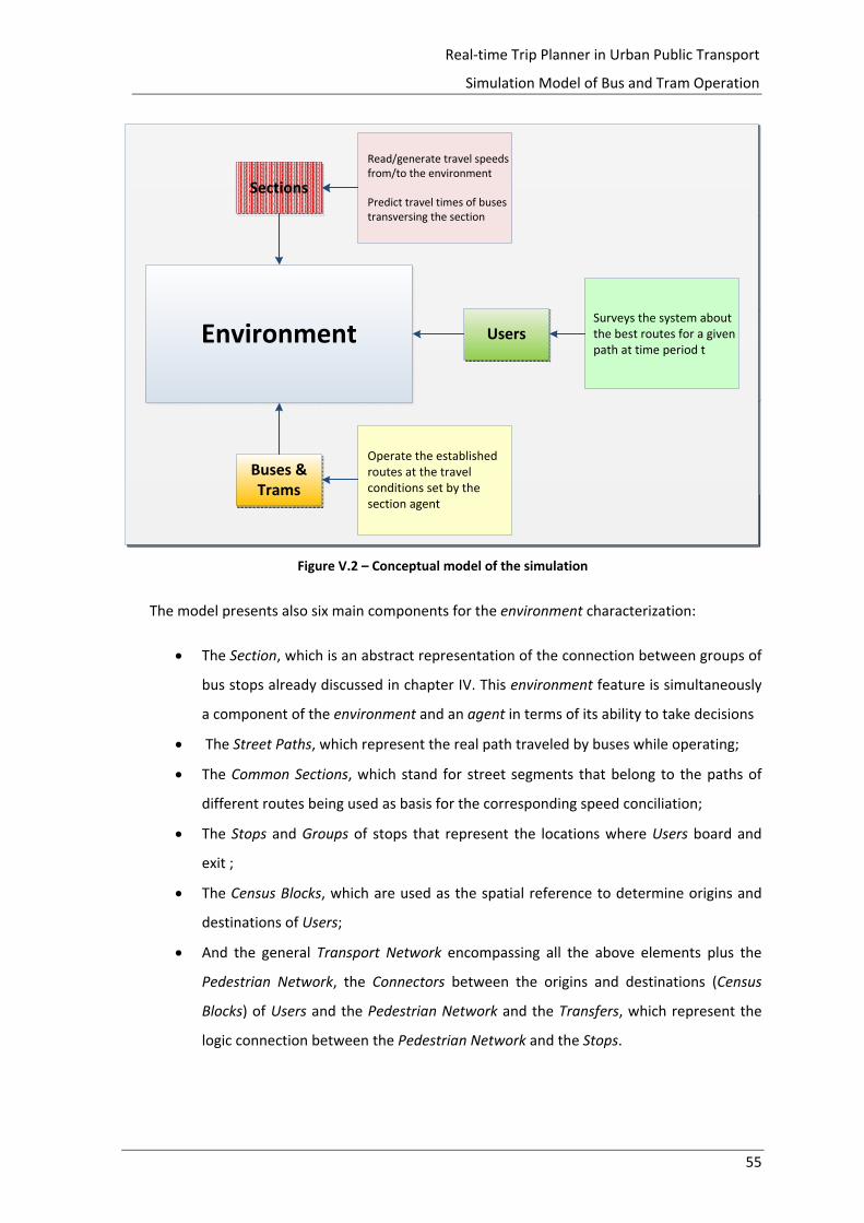
55



Environment Users

Buses & Trams

Sections

Read/generate travel speeds from/to the environment

Predict travel times of buses transversing the section

Surveys the system about the best routes for a given path at time period t

Operate the established routes at the travel conditions set by the section agent

Figure V.2 – Conceptual model of the simulation

The model presents also six main components for the environment characterization:

The Section, which is an abstract representation of the connection between groups of

bus stops already discussed in chapter IV. This environment feature is simultaneously

a component of the environment and an agent in terms of its ability to take decisions

The Street Paths, which represent the real path traveled by buses while operating;

The Common Sections, which stand for street segments that belong to the paths of

different routes being used as basis for the corresponding speed conciliation;

The Stops and Groups of stops that represent the locations where Users board and

exit ;

The Census Blocks, which are used as the spatial reference to determine origins and

destinations of Users;

And the general Transport Network encompassing all the above elements plus the

Pedestrian Network, the Connectors between the origins and destinations (Census

Blocks) of Users and the Pedestrian Network and the Transfers, which represent the

logic connection between the Pedestrian Network and the Stops.

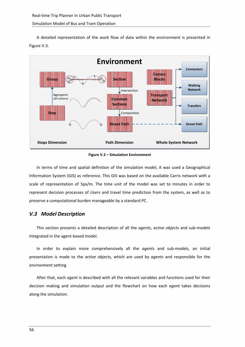
56



A detailed representation of the work flow of data within the environment is presented in

Figure V.3.

Environment

Transport Network

Stops Dimension Path Dimension Whole System Network

Walking Network

Connectors

Transfers

Street Path

Census BlocksSection

Street Path

Common Sections

Stop

Group

Aggregaton (30 meters)

Composition

Intersection

Figure V.3 – Simulation Environment

In terms of time and spatial definition of the simulation model, it was used a Geographical

Information System (GIS) as reference. This GIS was based on the available Carris network with a

scale of representation of 5px/m. The time unit of the model was set to minutes in order to

represent decision processes of Users and travel time prediction from the system, as well as to

preserve a computational burden manageable by a standard PC.

V.3 Model Description

This section presents a detailed description of all the agents, active objects and sub‐models

integrated in the agent‐based model.

In order to explain more comprehensively all the agents and sub‐models, an initial

presentation is made to the active objects, which are used by agents and responsible for the

environment setting.

After that, each agent is described with all the relevant variables and functions used for their

decision making and simulation output and the flowchart on how each agent takes decisions

along the simulation.

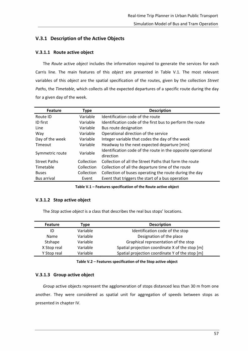
57



V.3.1 Description of the Active Objects

V.3.1.1 Route active object

The Route active object includes the information required to generate the services for each

Carris line. The main features of this object are presented in Table V.1. The most relevant

variables of this object are the spatial specification of the routes, given by the collection Street

Paths, the Timetable, which collects all the expected departures of a specific route during the day

for a given day of the week.

Feature Type Description

Route ID Variable Identification code of the route ID first Variable Identification code of the first bus to perform the route Line Variable Bus route designation Way Variable Operational direction of the service Day of the week Variable Integer variable that codes the day of the week Timeout Variable Headway to the next expected departure [min]

Symmetric route Variable Identification code of the route in the opposite operational direction

Street Paths Collection Collection of all the Street Paths that form the route Timetable Collection Collection of all the departure time of the route Buses Collection Collection of buses operating the route during the day Bus arrival Event Event that triggers the start of a bus operation

Table V.1 – Features specification of the Route active object

V.3.1.2 Stop active object

The Stop active object is a class that describes the real bus stops’ locations.


ID Variable Identification code of the stop Name Variable Designation of the place Stshape Variable Graphical representation of the stop

X Stop real Variable Spatial projection coordinate X of the stop [m] Y Stop real Variable Spatial projection coordinate Y of the stop [m]

Table V.2 – Features specification of the Stop active object

V.3.1.3 Group active object

Group active objects represent the agglomeration of stops distanced less than 30 m from one

another. They were considered as spatial unit for aggregation of speeds between stops as

presented in chapter IV.

58




X Variable X coordinate of the group centroid Y Variable Y coordinate of the group centroid

Table V.3 – Features specification of the Groups active object

V.3.1.4 Common Section active object

Common Section objects represent an overlap between sections and merge information to

compute travel times for the Street Paths. This class is responsible for the integration of speed

information among the different sections of the study area.


Section i Variable Section 1 Section j Variable Section 2 Distance Variable Euclidean distance between extremes Length Variable Real network distance [m] speed Variable Instant composite speed [px/min] Travel time Variable Instant travel time in section Estimated travel time Collection Collection of estimated travel times (6 periods) Predict travel time Event Event that triggers the update of travel time predictions

Update travel time Event Event that triggers the estimate of the instant composite speed

Table V.4 – Features specification of the Common Section active object

V.3.1.5 Street Path active object

The Street Path active objects assemble all the information of the transportation

infrastructure and services of the study area. Each active object represents a section of the real

physical transportation infrastructure for each route.


Route Variable Route that operates in the Street Path Section Variable Link to the corresponding section Sequence Variable Position in the bus stop sequence Stop i Variable Origin stop of the Street Path Stop j Variable Destination stop of the Street Path Distance Variable Euclidean distance between extremes [m] Length Variable Real network distance [m] Shaper Variable Graphical representation of the Street path Speed Variable Instant speed in the Street path [px/min] Travel time Variable Generated instant travel time [min] Zone Variable Zone to which the Street Path belongs Common section Collection Collection of the common sections of the Street Path Next buses Collection Collection of the registered bus passages Predicted bus Passages

Collection Collection of the predicted next bus passages

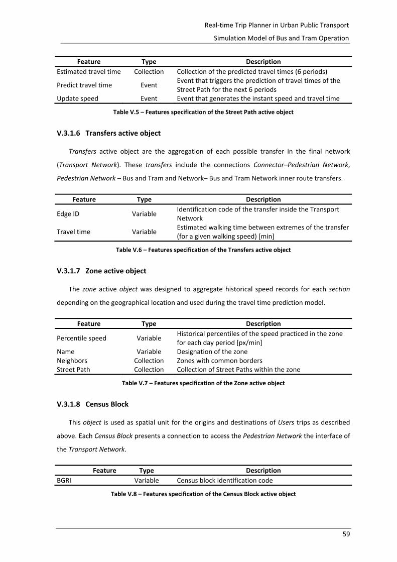
59




Estimated travel time Collection Collection of the predicted travel times (6 periods)

Predict travel time Event Event that triggers the prediction of travel times of the Street Path for the next 6 periods

Update speed Event Event that generates the instant speed and travel time

Table V.5 – Features specification of the Street Path active object

V.3.1.6 Transfers active object

Transfers active object are the aggregation of each possible transfer in the final network

(Transport Network). These transfers include the connections Connector–Pedestrian Network,

Pedestrian Network – Bus and Tram and Network– Bus and Tram Network inner route transfers.


Edge ID Variable Identification code of the transfer inside the Transport Network

Travel time Variable Estimated walking time between extremes of the transfer (for a given walking speed) [min]

Table V.6 – Features specification of the Transfers active object

V.3.1.7 Zone active object

The zone active object was designed to aggregate historical speed records for each section

depending on the geographical location and used during the travel time prediction model.


Percentile speed Variable Historical percentiles of the speed practiced in the zone for each day period [px/min]

Name Variable Designation of the zone Neighbors Collection Zones with common borders Street Path Collection Collection of Street Paths within the zone

Table V.7 – Features specification of the Zone active object

V.3.1.8 Census Block

This object is used as spatial unit for the origins and destinations of Users trips as described

above. Each Census Block presents a connection to access the Pedestrian Network the interface of

the Transport Network.


BGRI Variable Census block identification code

Table V.8 – Features specification of the Census Block active object

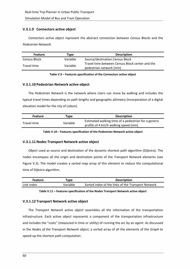
60



V.3.1.9 Connectors active object

Connectors active object represent the abstract connection between Census Blocks and the

Pedestrian Network.


Census Block Variable Source/destination Census Block

Travel time Variable Travel time between Census Block center and the pedestrian network [min]

Table V.9 – Features specification of the Connectors active object

V.3.1.10 Pedestrian Network active object

The Pedestrian Network is the network where Users can move by walking and includes the

typical travel times depending on path lengths and geographic altimetry (incorporation of a digital

elevation model for the city of Lisbon).


Travel time Variable Estimated walking time of a pedestrian for a generic profile of 4 km/h walking speed [min]

Table V.10 – Features specification of the Pedestrian Network active object

V.3.1.11 Nodes Transport Network active object

Object used as source and destination of the dynamic shortest path algorithm (Dijkstra). The

nodes encompass all the origin and destination points of the Transport Network elements (see

Figure V.3). The model creates a sorted map array of this element to reduce the computational

time of Dijkstra algorithm.


Link index Variable Sorted index of the links of the Transport Network

Table V.11 – Features specification of the Nodes Transport Network active object

V.3.1.12 Transport Network active object

The Transport Network active object assembles all the information of the transportation

infrastructure. Each active object represents a component of the transportation infrastructure

and includes the “costs” (measured in time or utility) of running the arc by an agent. As discussed

in the Nodes of the Transport Network object, a sorted array of all the elements of the Graph to

speed‐up the shortest path computation.

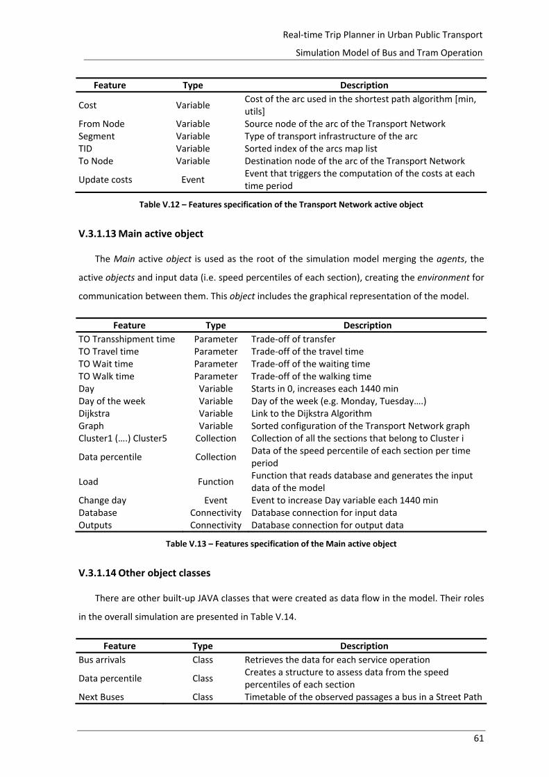
61




Cost Variable Cost of the arc used in the shortest path algorithm [min, utils]

From Node Variable Source node of the arc of the Transport Network Segment Variable Type of transport infrastructure of the arc TID Variable Sorted index of the arcs map list To Node Variable Destination node of the arc of the Transport Network

Update costs Event Event that triggers the computation of the costs at each time period

Table V.12 – Features specification of the Transport Network active object

V.3.1.13 Main active object

The Main active object is used as the root of the simulation model merging the agents, the

active objects and input data (i.e. speed percentiles of each section), creating the environment for

communication between them. This object includes the graphical representation of the model.


TO Transshipment time Parameter Trade‐off of transfer TO Travel time Parameter Trade‐off of the travel time TO Wait time Parameter Trade‐off of the waiting time TO Walk time Parameter Trade‐off of the walking time Day Variable Starts in 0, increases each 1440 min Day of the week Variable Day of the week (e.g. Monday, Tuesday….) Dijkstra Variable Link to the Dijkstra Algorithm Graph Variable Sorted configuration of the Transport Network graph Cluster1 (….) Cluster5 Collection Collection of all the sections that belong to Cluster i

Data percentile Collection Data of the speed percentile of each section per time period

Load Function Function that reads database and generates the input data of the model

Change day Event Event to increase Day variable each 1440 min Database Connectivity Database connection for input data Outputs Connectivity Database connection for output data

Table V.13 – Features specification of the Main active object

V.3.1.14 Other object classes

There are other built‐up JAVA classes that were created as data flow in the model. Their roles

in the overall simulation are presented in Table V.14.


Bus arrivals Class Retrieves the data for each service operation

Data percentile Class Creates a structure to assess data from the speed percentiles of each section

Next Buses Class Timetable of the observed passages a bus in a Street Path

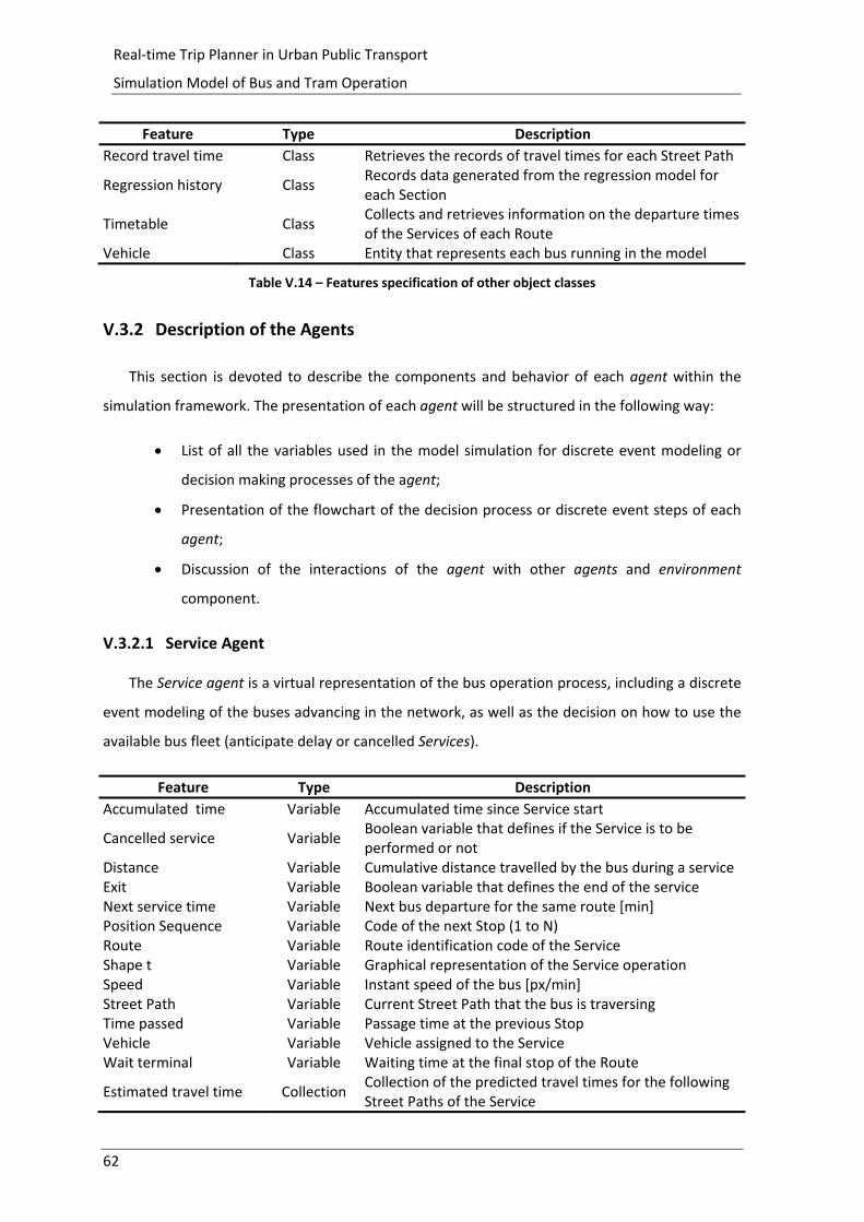
62




Record travel time Class Retrieves the records of travel times for each Street Path

Regression history Class Records data generated from the regression model for each Section

Timetable Class Collects and retrieves information on the departure times of the Services of each Route

Vehicle Class Entity that represents each bus running in the model

Table V.14 – Features specification of other object classes

V.3.2 Description of the Agents

This section is devoted to describe the components and behavior of each agent within the

simulation framework. The presentation of each agent will be structured in the following way:

List of all the variables used in the model simulation for discrete event modeling or

decision making processes of the agent;

Presentation of the flowchart of the decision process or discrete event steps of each

agent;

Discussion of the interactions of the agent with other agents and environment

component.

V.3.2.1 Service Agent

The Service agent is a virtual representation of the bus operation process, including a discrete

event modeling of the buses advancing in the network, as well as the decision on how to use the

available bus fleet (anticipate delay or cancelled Services).


Accumulated time Variable Accumulated time since Service start

Cancelled service Variable Boolean variable that defines if the Service is to be performed or not

Distance Variable Cumulative distance travelled by the bus during a service Exit Variable Boolean variable that defines the end of the service Next service time Variable Next bus departure for the same route [min] Position Sequence Variable Code of the next Stop (1 to N) Route Variable Route identification code of the Service Shape t Variable Graphical representation of the Service operation Speed Variable Instant speed of the bus [px/min] Street Path Variable Current Street Path that the bus is traversing Time passed Variable Passage time at the previous Stop Vehicle Variable Vehicle assigned to the Service Wait terminal Variable Waiting time at the final stop of the Route

Estimated travel time Collection Collection of the predicted travel times for the following Street Paths of the Service

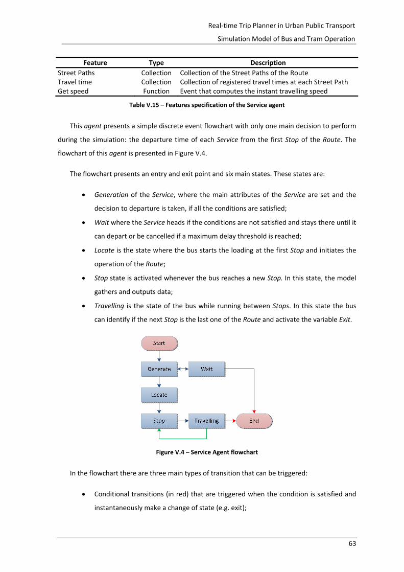
63




Street Paths Collection Collection of the Street Paths of the Route Travel time Collection Collection of registered travel times at each Street Path Get speed Function Event that computes the instant travelling speed

Table V.15 – Features specification of the Service agent

This agent presents a simple discrete event flowchart with only one main decision to perform

during the simulation: the departure time of each Service from the first Stop of the Route. The

flowchart of this agent is presented in Figure V.4.

The flowchart presents an entry and exit point and six main states. These states are:

Generation of the Service, where the main attributes of the Service are set and the

decision to departure is taken, if all the conditions are satisfied;

Wait where the Service heads if the conditions are not satisfied and stays there until it

can depart or be cancelled if a maximum delay threshold is reached;

Locate is the state where the bus starts the loading at the first Stop and initiates the

operation of the Route;

Stop state is activated whenever the bus reaches a new Stop. In this state, the model

gathers and outputs data;

Travelling is the state of the bus while running between Stops. In this state the bus

can identify if the next Stop is the last one of the Route and activate the variable Exit.

Figure V.4 – Service Agent flowchart

In the flowchart there are three main types of transition that can be triggered:

Conditional transitions (in red) that are triggered when the condition is satisfied and

instantaneously make a change of state (e.g. exit);

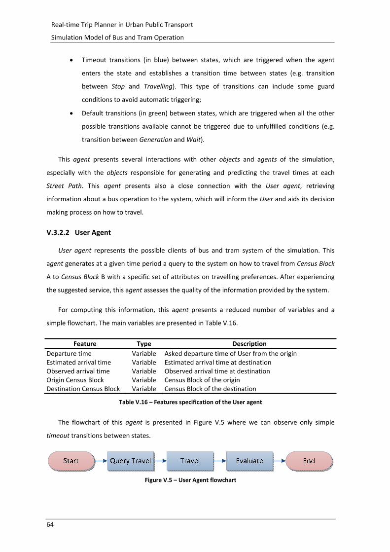
64



Timeout transitions (in blue) between states, which are triggered when the agent

enters the state and establishes a transition time between states (e.g. transition

between Stop and Travelling). This type of transitions can include some guard

conditions to avoid automatic triggering;

Default transitions (in green) between states, which are triggered when all the other

possible transitions available cannot be triggered due to unfulfilled conditions (e.g.

transition between Generation and Wait).

This agent presents several interactions with other objects and agents of the simulation,

especially with the objects responsible for generating and predicting the travel times at each

Street Path. This agent presents also a close connection with the User agent, retrieving

information about a bus operation to the system, which will inform the User and aids its decision

making process on how to travel.

V.3.2.2 User Agent

User agent represents the possible clients of bus and tram system of the simulation. This

agent generates at a given time period a query to the system on how to travel from Census Block

A to Census Block B with a specific set of attributes on travelling preferences. After experiencing

the suggested service, this agent assesses the quality of the information provided by the system.

For computing this information, this agent presents a reduced number of variables and a

simple flowchart. The main variables are presented in Table V.16.


Departure time Variable Asked departure time of User from the origin Estimated arrival time Variable Estimated arrival time at destination Observed arrival time Variable Observed arrival time at destination Origin Census Block Variable Census Block of the origin Destination Census Block Variable Census Block of the destination

Table V.16 – Features specification of the User agent

The flowchart of this agent is presented in Figure V.5 where we can observe only simple

timeout transitions between states.

Figure V.5 – User Agent flowchart

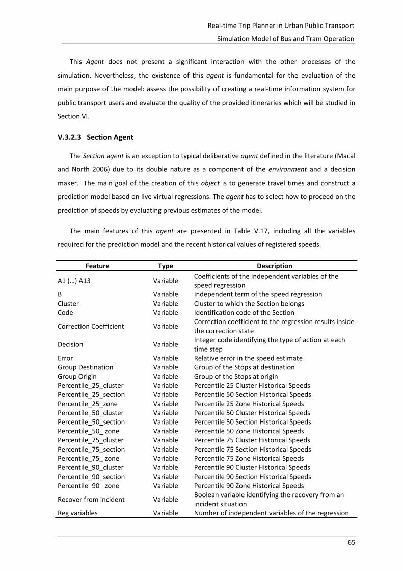
65



This Agent does not present a significant interaction with the other processes of the

simulation. Nevertheless, the existence of this agent is fundamental for the evaluation of the

main purpose of the model: assess the possibility of creating a real‐time information system for

public transport users and evaluate the quality of the provided itineraries which will be studied in

Section VI.

V.3.2.3 Section Agent

The Section agent is an exception to typical deliberative agent defined in the literature (Macal

and North 2006) due to its double nature as a component of the environment and a decision

maker. The main goal of the creation of this object is to generate travel times and construct a

prediction model based on live virtual regressions. The agent has to select how to proceed on the

prediction of speeds by evaluating previous estimates of the model.

The main features of this agent are presented in Table V.17, including all the variables

required for the prediction model and the recent historical values of registered speeds.


A1 (…) A13 Variable Coefficients of the independent variables of the speed regression

B Variable Independent term of the speed regression Cluster Variable Cluster to which the Section belongs Code Variable Identification code of the Section

Correction Coefficient Variable Correction coefficient to the regression results inside the correction state

Decision Variable Integer code identifying the type of action at each time step

Error Variable Relative error in the speed estimate Group Destination Variable Group of the Stops at destination Group Origin Variable Group of the Stops at origin Percentile_25_cluster Variable Percentile 25 Cluster Historical Speeds Percentile_25_section Variable Percentile 50 Section Historical Speeds Percentile_25_zone Variable Percentile 25 Zone Historical Speeds Percentile_50_cluster Variable Percentile 50 Cluster Historical Speeds Percentile_50_section Variable Percentile 50 Section Historical Speeds Percentile_50_ zone Variable Percentile 50 Zone Historical Speeds Percentile_75_cluster Variable Percentile 75 Cluster Historical Speeds Percentile_75_section Variable Percentile 75 Section Historical Speeds Percentile_75_ zone Variable Percentile 75 Zone Historical Speeds Percentile_90_cluster Variable Percentile 90 Cluster Historical Speeds Percentile_90_section Variable Percentile 90 Section Historical Speeds Percentile_90_ zone Variable Percentile 90 Zone Historical Speeds

Recover from incident Variable Boolean variable identifying the recovery from an incident situation

Reg variables Variable Number of independent variables of the regression

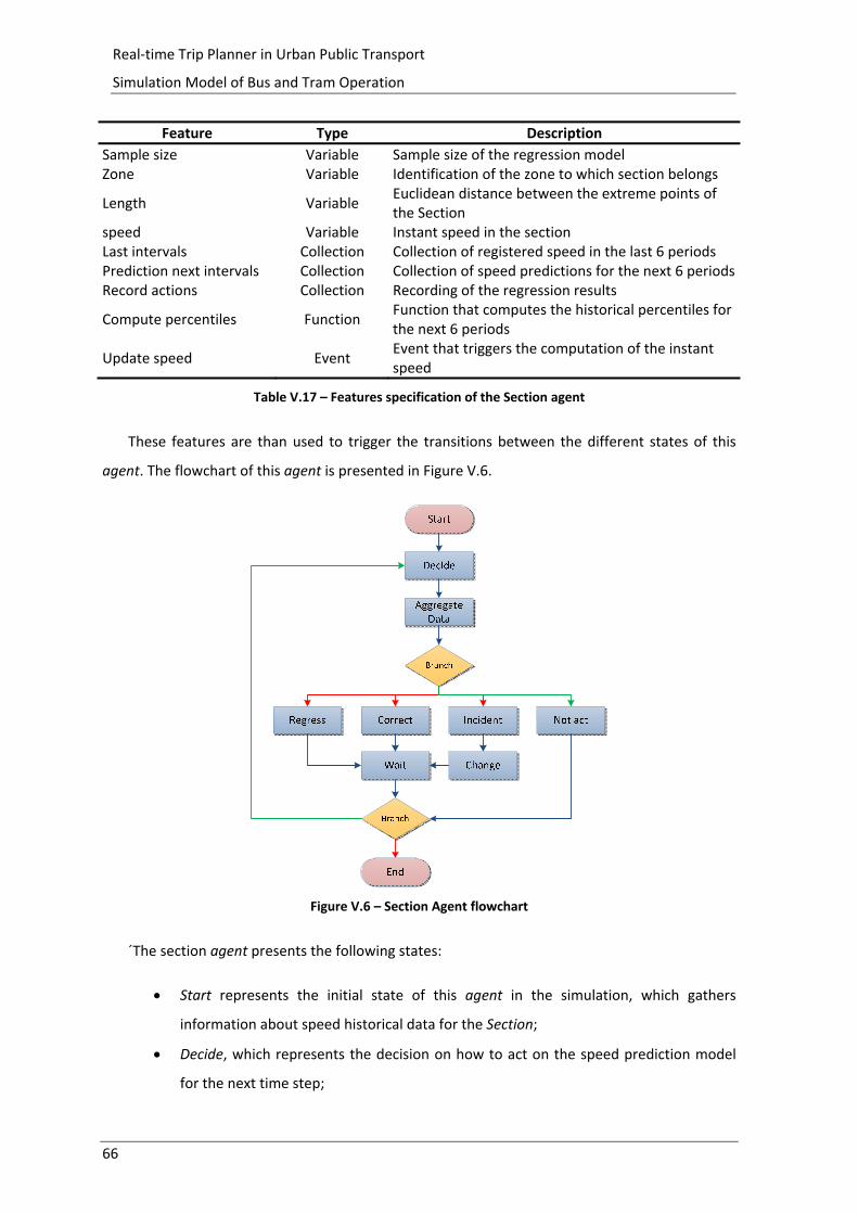
66




Sample size Variable Sample size of the regression model Zone Variable Identification of the zone to which section belongs

Length Variable Euclidean distance between the extreme points of the Section

speed Variable Instant speed in the section Last intervals Collection Collection of registered speed in the last 6 periods Prediction next intervals Collection Collection of speed predictions for the next 6 periodsRecord actions Collection Recording of the regression results

Compute percentiles Function Function that computes the historical percentiles for the next 6 periods

Update speed Event Event that triggers the computation of the instant speed

Table V.17 – Features specification of the Section agent

These features are than used to trigger the transitions between the different states of this

agent. The flowchart of this agent is presented in Figure V.6.

Figure V.6 – Section Agent flowchart

´The section agent presents the following states:

Start represents the initial state of this agent in the simulation, which gathers

information about speed historical data for the Section;

Decide, which represents the decision on how to act on the speed prediction model

for the next time step;

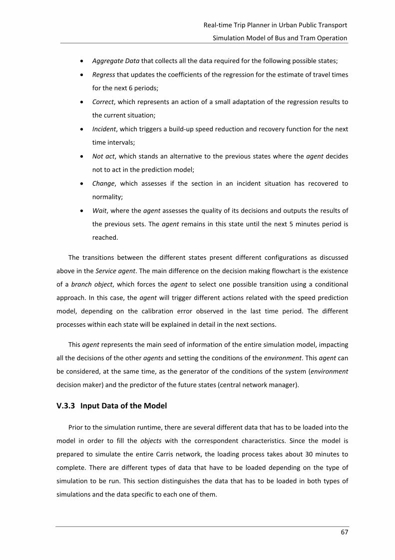
67



Aggregate Data that collects all the data required for the following possible states;

Regress that updates the coefficients of the regression for the estimate of travel times

for the next 6 periods;

Correct, which represents an action of a small adaptation of the regression results to

the current situation;

Incident, which triggers a build‐up speed reduction and recovery function for the next

time intervals;

Not act, which stands an alternative to the previous states where the agent decides

not to act in the prediction model;

Change, which assesses if the section in an incident situation has recovered to

normality;

Wait, where the agent assesses the quality of its decisions and outputs the results of

the previous sets. The agent remains in this state until the next 5 minutes period is

reached.

The transitions between the different states present different configurations as discussed

above in the Service agent. The main difference on the decision making flowchart is the existence

of a branch object, which forces the agent to select one possible transition using a conditional

approach. In this case, the agent will trigger different actions related with the speed prediction

model, depending on the calibration error observed in the last time period. The different

processes within each state will be explained in detail in the next sections.

This agent represents the main seed of information of the entire simulation model, impacting

all the decisions of the other agents and setting the conditions of the environment. This agent can

be considered, at the same time, as the generator of the conditions of the system (environment

decision maker) and the predictor of the future states (central network manager).

V.3.3 Input Data of the Model

Prior to the simulation runtime, there are several different data that has to be loaded into the

model in order to fill the objects with the correspondent characteristics. Since the model is

prepared to simulate the entire Carris network, the loading process takes about 30 minutes to

complete. There are different types of data that have to be loaded depending on the type of

simulation to be run. This section distinguishes the data that has to be loaded in both types of

simulations and the data specific to each one of them.

68



V.3.3.1 General Data

There are objects that represent the physical networks included in the model and historical

speed records. Since they are static and common to both simulation types, the information

associated with each one is always loaded. These features are:

Network geographical characteristics (that include bus and tram network, pedestrian

network, connectors Census Block – pedestrian network, possible transfers) – 59,388

links and 22,113 nodes;

Set of available bus lines – 174 elements (86x2 bidirectional, 2 circular);

Bus line Street Paths – 4,802 elements;

Sections – 2,780 elements;

Common sections – 6463 elements;

Historical speed percentiles of each section for each day 5 minute’s period –

2,780x4x288=3,202,560 elements;

Census Blocks – 4,390 elements.

V.3.3.2 Synthetic Day Speeds Generation

When there is no real data to measure the practiced speeds and travel times in the network,

the model generates a synthetic day of operation of the Carris network. In this mode, the model

generates travel time speeds and uses as operational reference the stated Carris timetables of

2011, adapted to the period of operation (2009‐2010). The features required to set the

operational patterns of a regular day are:

Number of vehicles assigned to each Service (based on the example log‐file of the

4th of April 2010);

Official Carris timetables to trigger the Services.

The resulting operation may not fully comply with the stated official timetables due to

services delays that can result in services suspension or bunching in departures of the same

services.

V.3.3.3 Log‐file Load

When the model is ran with registers from a real day of operation, there is no need to

generate synthetically travel times in sections and therefore the features are directly imported to

the model from the Carris log‐file. The features loaded are:

69



Effective bus and tram departures;

Registered travel time.

V.4 Computation of Travel Times in the Simulation Environment

Travel time prediction is presented in two distinct phases. Firstly, the mechanism created to

generate travel times in each section is presented, where the section to be computed will be

associated to an AnyLogic Agent variable (dynamic with flowchart behavior). This first function

may only be triggered when there is no real data being collected from the network. In one of the

examples presented below for a real operation day of Carris in the city of Lisbon, this function

aggregates information to compute real travel times registered by bus and tram passages.

Secondly, the concept underlying the prediction algorithm is presented. Which, when and how

data is used and communicated to the other elements of the environment and agents.

V.4.1 Generation of Speeds and Travel Times in the Simulation Environment

The generation of travel times in the simulation environment was based on the historical

speed profiles for each Section developed in Chapter IV. These speed profiles were computed in 5

minute periods.

The developed procedure to generate travel times is based on a three random components

model:

One relative to the impact of the historical data on the generation of the next period

instant speed;

Another devoted to the last observed speeds in the Section;

And a third component relative to a random variation of the instant speed. This

component was modeled through the statistical distribution of the speeds observed

in the sample. This random component at this stage of the study was based on the

entire network speed profile and follows a normal distribution with an average speed

of 23.01 km/h and a standard deviation of 5.13 km/h.

The final speed estimate results of a linear combination of these three components.

The model contains in total 19 variables, whose weight in the final linear model is randomly

generated for each period to ensure independency between consecutive speed estimates. These

variables are presented in Table V.18. Within each group the weights of each variable for the

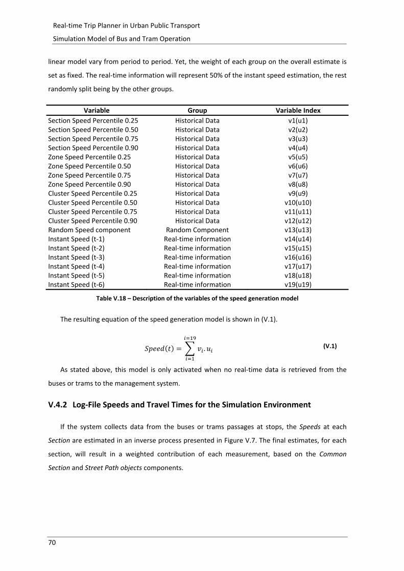
70



linear model vary from period to period. Yet, the weight of each group on the overall estimate is

set as fixed. The real‐time information will represent 50% of the instant speed estimation, the rest

randomly split being by the other groups.

Variable Group Variable Index

Section Speed Percentile 0.25 Historical Data v1(u1) Section Speed Percentile 0.50 Historical Data v2(u2) Section Speed Percentile 0.75 Historical Data v3(u3) Section Speed Percentile 0.90 Historical Data v4(u4) Zone Speed Percentile 0.25 Historical Data v5(u5) Zone Speed Percentile 0.50 Historical Data v6(u6) Zone Speed Percentile 0.75 Historical Data v7(u7) Zone Speed Percentile 0.90 Historical Data v8(u8) Cluster Speed Percentile 0.25 Historical Data v9(u9) Cluster Speed Percentile 0.50 Historical Data v10(u10) Cluster Speed Percentile 0.75 Historical Data v11(u11) Cluster Speed Percentile 0.90 Historical Data v12(u12) Random Speed component Random Component v13(u13) Instant Speed (t‐1) Real‐time information v14(u14) Instant Speed (t‐2) Real‐time information v15(u15) Instant Speed (t‐3) Real‐time information v16(u16) Instant Speed (t‐4) Real‐time information v17(u17) Instant Speed (t‐5) Real‐time information v18(u18) Instant Speed (t‐6) Real‐time information v19(u19)

Table V.18 – Description of the variables of the speed generation model

The resulting equation of the speed generation model is shown in (V.1).

. (V.1)

As stated above, this model is only activated when no real‐time data is retrieved from the

buses or trams to the management system.

V.4.2 Log‐File Speeds and Travel Times for the Simulation Environment

If the system collects data from the buses or trams passages at stops, the Speeds at each

Section are estimated in an inverse process presented in Figure V.7. The final estimates, for each

section, will result in a weighted contribution of each measurement, based on the Common

Section and Street Path objects components.

71



Figure V.7 – Process of computation of Instant Section Speed

This process results in an equation for each section based on the relation between Street

Paths, Common Sections and Sections. The travel time in a section can be then estimated by:

∑ . .

∑

(V.2)

This procedure generates a back propagation from Street Paths to Common Sections, and

from Common Sections to Sections, where the prediction of travel time and speed is performed,

as presented in the next section.

V.4.3 Prediction of Speeds and Travel Times in the Simulation Environment

The prediction of speeds and travel times within the Section agent was formulated as a cyclic

routine that evaluates the estimates every time period. The process stabilizes when the error

associated with the prediction is less than 5%. The prediction is based on linear regressions that

depend on data availability, last iteration error, Section and zone typical speed values for the

period to compute.

V.4.3.1 Model flowchart

To predict speeds and travel times, a routine was created in order to repeatedly evaluate

every 5 minutes the accuracy of the prediction and act according to the results (Figure V.8).

If the estimate of the last period does not satisfy the relative error threshold (5%), the model

will correct the prediction. These corrections can trigger, depending on the level of relative error,

three different functions: compute a new regression, make a correction to the regression

estimates or trigger a build‐up event for incidents. The established thresholds for these functions

were:

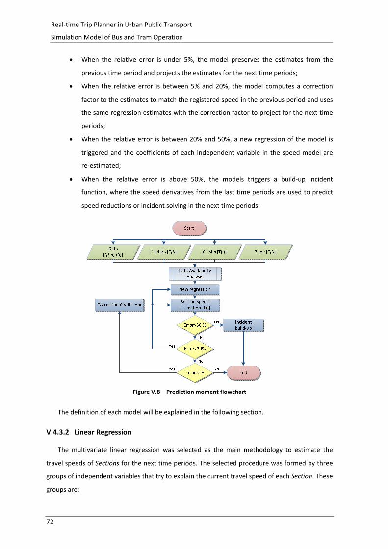
72



When the relative error is under 5%, the model preserves the estimates from the

previous time period and projects the estimates for the next time periods;

When the relative error is between 5% and 20%, the model computes a correction

factor to the estimates to match the registered speed in the previous period and uses

the same regression estimates with the correction factor to project for the next time

periods;

When the relative error is between 20% and 50%, a new regression of the model is

triggered and the coefficients of each independent variable in the speed model are

re‐estimated;

When the relative error is above 50%, the models triggers a build‐up incident

function, where the speed derivatives from the last time periods are used to predict

speed reductions or incident solving in the next time periods.

Figure V.8 – Prediction moment flowchart

The definition of each model will be explained in the following section.

V.4.3.2 Linear Regression

The multivariate linear regression was selected as the main methodology to estimate the

travel speeds of Sections for the next time periods. The selected procedure was formed by three

groups of independent variables that try to explain the current travel speed of each Section. These

groups are:

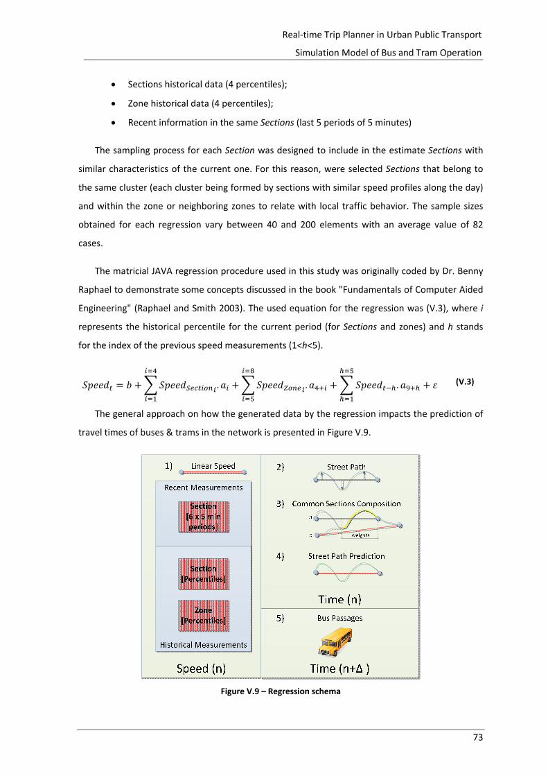
73



Sections historical data (4 percentiles);

Zone historical data (4 percentiles);

Recent information in the same Sections (last 5 periods of 5 minutes)

The sampling process for each Section was designed to include in the estimate Sections with

similar characteristics of the current one. For this reason, were selected Sections that belong to

the same cluster (each cluster being formed by sections with similar speed profiles along the day)

and within the zone or neighboring zones to relate with local traffic behavior. The sample sizes

obtained for each regression vary between 40 and 200 elements with an average value of 82

cases.

The matricial JAVA regression procedure used in this study was originally coded by Dr. Benny

Raphael to demonstrate some concepts discussed in the book "Fundamentals of Computer Aided

Engineering" (Raphael and Smith 2003). The used equation for the regression was (V.3), where i

represents the historical percentile for the current period (for Sections and zones) and h stands

for the index of the previous speed measurements (1<h<5).

. . . (V.3)

The general approach on how the generated data by the regression impacts the prediction of

travel times of buses & trams in the network is presented in Figure V.9.

Figure V.9 – Regression schema

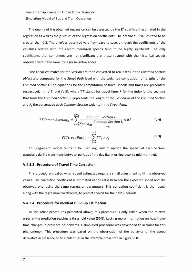
74



The quality of the obtained regression can be assessed by the R2 coefficient estimated in the

regression as well as the p‐values of the regression coefficients. The obtained R2 values tend to be

greater than 0.8. The p‐values observed vary from case to case, although the coefficients of the

variables related with the recent measured speeds tend to be highly significant. The only

coefficients that sometimes are not significant are those related with the historical speeds

observed within the same zone (or neighbor zones).

The linear estimates for the Section are then converted to real paths in the Common Section

object and computed for the Street Path level with the weighted composition of lengths of the

Common Sections. The equations for the computation of travel speeds and times are presented,

respectively, in (V.4) and (V.5), where stands for travel time, k for the index of the sections

that form the Common Section, represents the length of the Section or of the Common Section

and the percentage each Common Section weights in the Street Path.

0.5 (V.4)

(V.5)

This regression model tends to be used regularly to update the speeds of each Section,

especially during transitions between periods of the day (i.e. morning peak to mid‐morning).

V.4.3.3 Procedure of Travel Time Correction

This procedure is called when speed estimates require a small adjustment to fit the observed

values. The correction coefficient is estimated as the ratio between the expected speed and the

observed one, using the same regression parameters. This correction coefficient is then used,

along with the regression coefficients, to predict speeds for the next 6 periods.

V.4.3.4 Procedure for Incident Build‐up Estimation

As the other procedures presented above, this procedure is only called when the relative

error in the prediction reaches a threshold value (50%). Lacking more information on how travel

time changes in presence of incidents, a simplified procedure was developed to account for this

phenomenon. This procedure was based on the observation of the behavior of the speed

derivative in presence of an incident, as in the example presented in Figure V.10.

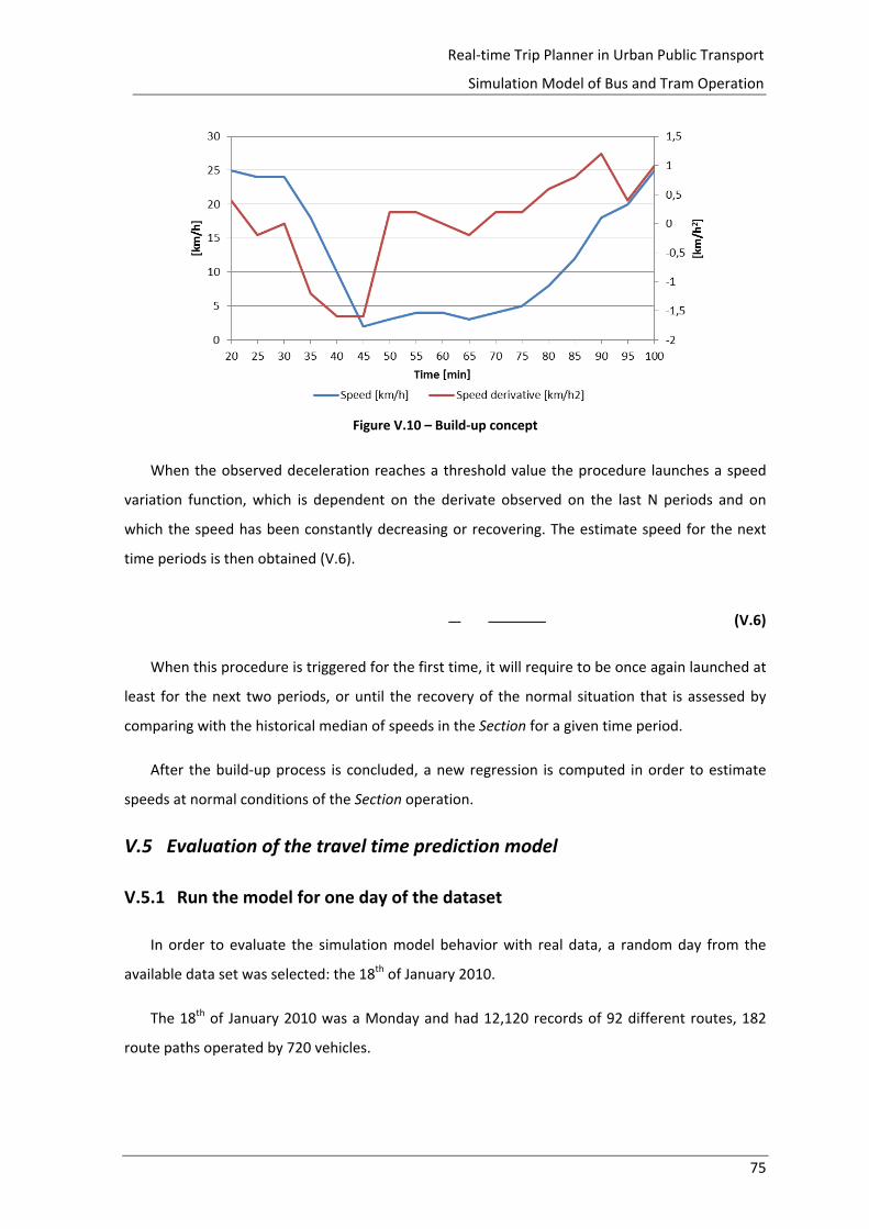
75



Figure V.10 – Build‐up concept

When the observed deceleration reaches a threshold value the procedure launches a speed

variation function, which is dependent on the derivate observed on the last N periods and on

which the speed has been constantly decreasing or recovering. The estimate speed for the next

time periods is then obtained (V.6).

(V.6)

When this procedure is triggered for the first time, it will require to be once again launched at

least for the next two periods, or until the recovery of the normal situation that is assessed by

comparing with the historical median of speeds in the Section for a given time period.

After the build‐up process is concluded, a new regression is computed in order to estimate

speeds at normal conditions of the Section operation.

V.5 Evaluation of the travel time prediction model

V.5.1 Run the model for one day of the dataset

In order to evaluate the simulation model behavior with real data, a random day from the

available data set was selected: the 18th of January 2010.

The 18th of January 2010 was a Monday and had 12,120 records of 92 different routes, 182

route paths operated by 720 vehicles.

76



V.5.1.1 Test constraints

Since there were some inconsistencies in data availability of paths and the Carris log‐file data

base, this assessment was adapted to the current conditions, which lead to a reduction of the

available sample. These reductions were due to:

Incompatibilities in stops and sections of the dataset with the network used in the

model, 94 records had to be ignored;

The existence of services already operating on the database that started before 00:00

and, therefore, 50 more records had to be ignored.

Anomalies on the regular path of some Services, which lead to a suppression of 388

records.

Summarizing, given the constraints above mentioned only 96% of the records from the 18th of

January 2010 were considered.

V.5.1.2 Evaluation of exclusive off‐line historical data in the model to predict speed

and travel times

In order to test the relevance of developing a real‐time prediction model, a test was

performed to the ability of the historical data median for a given section to predict the registered

travel times. The first iteration of the test included all the valid records. The estimates were

computed and a regression was made in order to fit them into the real speeds observed on the

18th of January 2010.

The regression produces a very low R2 (only 0.239) which reflects the lack of accuracy of the

predictions made using only the median percentile historical data as inputs for the model. While

this coefficient of determination is low, it is interesting to notice that the regression coefficients

obtained were positive, which means that the predictions tend to under‐estimate travel times.

The second iteration of the test considered the sum of predictions (computed as described in

V.4.3) for each Section that composes each complete Route. This regression presented a

significant R2 value of 0.7542 (see Figure V.11).

77



Figure V.11 – Estimated travel times median Section values versus Real travel times

Although the regression returns a high coefficient of determination, the travel time estimates

are approximately 20% above the real registered ones and the distribution of registered values

present a high dispersion of points surrounding the estimated regression line. This dispersion is

even larger in intermediate values, where more registers are available (40‐100 min).

V.5.1.3 Evaluation of real‐time data in the model to predict speed and travel times

To evaluate the accuracy gain in predictions made by adding real‐time data, it was performed

a second test also based on the 18th of January 2010. The main difference, between this test and

the one described above, is the inclusion of a dynamic prediction model that uses the travel times

registered in the six 5 minute periods prior to the prediction instant and not only historical

median values.

The procedure used to estimate speeds at the Sections level from detection of travel times at

the Street Paths was discussed V.4.1.

The obtained results from this analysis showed a completely different pattern from the

relation between real and estimated routes travel times. While travel times estimated by the

historical median of each Section tended to be higher than the observed values, the developed

prediction models tend to accurately estimate travel times.

y = 0,7289x + 3,9904R² = 0,7542

0

20

40

60

80

100

120

140

0 20 40 60 80 100 120

Real travel tim

e [min]

Estimated travel times of the services or segments of services

Data Points Trend Line (Data Points)

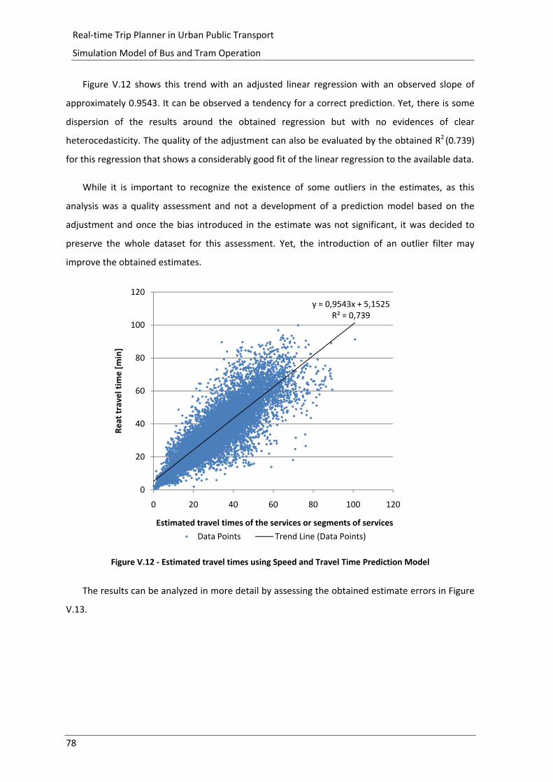
78



Figure V.12 shows this trend with an adjusted linear regression with an observed slope of

approximately 0.9543. It can be observed a tendency for a correct prediction. Yet, there is some

dispersion of the results around the obtained regression but with no evidences of clear

heterocedasticity. The quality of the adjustment can also be evaluated by the obtained R2 (0.739)

for this regression that shows a considerably good fit of the linear regression to the available data.

While it is important to recognize the existence of some outliers in the estimates, as this

analysis was a quality assessment and not a development of a prediction model based on the

adjustment and once the bias introduced in the estimate was not significant, it was decided to

preserve the whole dataset for this assessment. Yet, the introduction of an outlier filter may

improve the obtained estimates.

Figure V.12 ‐ Estimated travel times using Speed and Travel Time Prediction Model

The results can be analyzed in more detail by assessing the obtained estimate errors in Figure

V.13.

y = 0,9543x + 5,1525R² = 0,739

0

20

40

60

80

100

120

0 20 40 60 80 100 120

Reat travel tim

e [min]

Estimated travel times of the services or segments of services

Data Points Trend Line (Data Points)

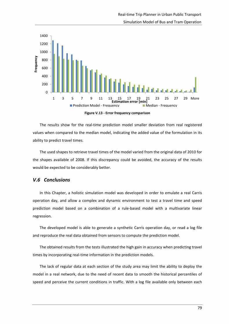
79



Figure V.13 ‐ Error frequency comparison

The results show for the real‐time prediction model smaller deviation from real registered

values when compared to the median model, indicating the added value of the formulation in its

ability to predict travel times.

The used shapes to retrieve travel times of the model varied from the original data of 2010 for

the shapes available of 2008. If this discrepancy could be avoided, the accuracy of the results

would be expected to be considerably better.

V.6 Conclusions

In this Chapter, a holistic simulation model was developed in order to emulate a real Carris

operation day, and allow a complex and dynamic environment to test a travel time and speed

prediction model based on a combination of a rule‐based model with a multivariate linear

regression.

The developed model is able to generate a synthetic Carris operation day, or read a log file

and reproduce the real data obtained from sensors to compute the prediction model.

The obtained results from the tests illustrated the high gain in accuracy when predicting travel

times by incorporating real‐time information in the prediction models.

The lack of regular data at each section of the study area may limit the ability to deploy the

model in a real network, due to the need of recent data to smooth the historical percentiles of

speed and perceive the current conditions in traffic. With a log file available only between each

0

200

400

600

800

1000

1200

1400

1 3 5 7 9 11 13 15 17 19 21 23 25 27 29 More

Frequency

Estimation error [min]Prediction Model ‐ Frequency Median ‐ Frequency

80



bus stop, this might be insufficient for an accurate estimate of the expected travel times for the

next 60 minutes.

This limitation can be easily surpassed if a continuous log file (registers every 30 seconds) is

available, which may allow to switch the unit of prediction from a Section to a real road network

arc.

81


Trip‐Planner

VI Trip‐Planner

VI.1 Introduction

In this section will be illustrated the potential application of the model developed for a real

world trip‐planner. This corresponds to the process from the instant when the system receives

short and medium term queries till the system returns the stop towards which the user should

walk to and the estimated travel times and possible transfers for the desired trip.

An ideal trip‐planner would provide to the end‐user:

Real‐time information on the best stop to start the trip;

Real‐time information on next bus passages at the best stop to start the trip;

Walking time to the stop;

Expected travel time updatable during the trip (possibly a countdown);

Number of transfers;

Waiting time on transfers;

Countdown to the next stop;

Expected walking time from the last stop to the destination;

Identification of alternative routes in case of incident (during the trip);

Best transport mode or combinations of modes to complete the journey;

Real‐time weather conditions and forecasts for at least one day;

Costs expected;

Different trip‐plans sorted by user preferences (e.g. minimum number of transfers,

preferred mode, etc.)

Real‐time information on incidents located in subsequent steps of the mobility chain;

Information on the level of occupancy of the bus, tram, subway, etc.;

It will also be made a general description of the algorithm behind this procedure: a Dijkstra

Algorithm with scheduled services. Some adaptation to the original formulations will be

introduced in order to support the inclusion of this methodology in the prediction model. Finally,

the model will be tested using a synthetic population of clients and the reliability of the estimated

trip plan is going to be evaluated by comparison with the observed travel times.

82


Trip‐Planner

The presented test will not present all the potentialities described above. Nevertheless, it

presents already some of the main features required for a trip‐planner to operate satisfactorily.

VI.2 Dijkstra Algorithm and Adaptations

Dijkstra’s algorithm was conceived by Dutch computer scientist Edsger Dijkstra in 1956 and

published in 1959 (Barbehenn 1998). Dijkstra algorithm is a graph search algorithm that solves the

single‐source shortest path problem for a graph with nonnegative edge path costs, producing a

shortest path tree. This algorithm is often used in routing and as a subroutine in other graph

algorithms.

For a given source vertex (node) in the graph, the algorithm finds the path with lowest cost

(i.e. the shortest path) between that vertex and every other vertex. It can also be used for finding

costs of shortest paths from a single vertex to a single destination vertex by stopping the

algorithm once the shortest path to the destination vertex has been determined. For example, if

the vertices of the graph represent stops and edge path costs represent travel times between

pairs of stops connected by a direct road, Dijkstra's algorithm can be used to find the shortest

route between one stop and all other stops.

In a public transport network defined by the service headways, the original formulation of this

algorithm no longer produces shorter paths because the axiom of separability of the optimal

shortest path in optimal sub‐paths between intermediate nodes no longer applies. This is due to

the fact that the quickest path to an intermediate node may correspond to using a direct service

there but imply a transfer to another service on the way to the end node, whereas the quickest

path to the end node uses a slower service to the intermediate node, but then goes on in the

same service to the end node. However, this problem does not occur if the public transport

network is described with scheduled services, as it is here the case, and so the basic concepts of

the algorithm can be used, with only minor adaptations to the definition of links as services with a

precise location and time of the start and end nodes(Merrifield 2004).

This algorithm was programmed in JAVA using a previous code version from the traditional

Dijkstra algorithm applied in a shared taxi simulation model (Martínez, Correia et al. 2011).

Dijkstra algorithm was used in the trip‐planner by introducing “costs” in the arcs, including

different types of travel times that were converted to a utility measure, using trade‐off values

estimated between travel time and waiting time (Martínez, Correia et al. 2011). The obtained

path and utility estimate are then converted, in each iteration, to equivalent travel times to be

83


Trip‐Planner

communicated to the User. The purpose of this conversion is the evaluation of which of the

different possible total Nodes Transport Network (see V.3.1.11) sequence returns the shortest

total travel time.

VI.3 Test the trip‐planner for short and medium term queries

In order to get the best routes by bus and/or tram at a given period of the day, standard

parameters for the characterization of the User were used in terms of average walking speed and

willingness to perform an extra transfer. A query triggers the prediction model that, using and

adapted Dijkstra model with node and section schedule, computes the equivalent shortest path to

complete the desired trip.

VI.3.1 Test for a synthetic population of clients to measure the agenda

adjustment

In this section, a test is presented for the trip‐planner model running a synthetic population of

clients which query the system for short and medium term estimates. It will be evaluated how the

predictions fit into their agenda.

19 stops have been selected in order to perform a set of query tests to evaluate how the

prediction model responds to requests on different places of the city and with different possible

combinations of bus lines. A simple stop selection principle was defined: the stops should be

homogenously distributed along the city and they should be located in easily accessible points by

public transport (i.e. with multiple bus lines available). The location of the stops selected is

presented in Figure VI.1.

Figure VI.1 ‐ Test Source/Destination Stops

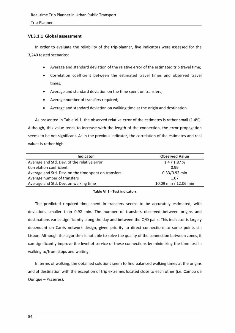
84


Trip‐Planner

VI.3.1.1 Global assessment

In order to evaluate the reliability of the trip‐planner, five indicators were assessed for the

3,240 tested scenarios:

Average and standard deviation of the relative error of the estimated trip travel time;

Correlation coefficient between the estimated travel times and observed travel

times;

Average and standard deviation on the time spent on transfers;

Average number of transfers required;

Average and standard deviation on walking time at the origin and destination.

As presented in Table VI.1, the observed relative error of the estimates is rather small (1.4%).

Although, this value tends to increase with the length of the connection, the error propagation

seems to be not significant. As in the previous indicator, the correlation of the estimates and real

values is rather high.

Indicator Observed Value

Average and Std. Dev. of the relative error 1.4 / 1.87 % Correlation coefficient 0.99 Average and Std. Dev. on the time spent on transfers 0.33/0.92 min Average number of transfers 1.07 Average and Std. Dev. on walking time 10.09 min / 12.06 min

Table VI.1 ‐ Test indicators

The predicted required time spent in transfers seems to be accurately estimated, with

deviations smaller than 0.92 min. The number of transfers observed between origins and

destinations varies significantly along the day and between the O/D pairs. This indicator is largely

dependent on Carris network design, given priority to direct connections to some points sin

Lisbon. Although the algorithm is not able to solve the quality of the connection between zones, it

can significantly improve the level of service of these connections by minimizing the time lost in

walking to/from stops and waiting.

In terms of walking, the obtained solutions seem to find balanced walking times at the origins

and at destination with the exception of trip extremes located close to each other (i.e. Campo de

Ourique – Prazeres).

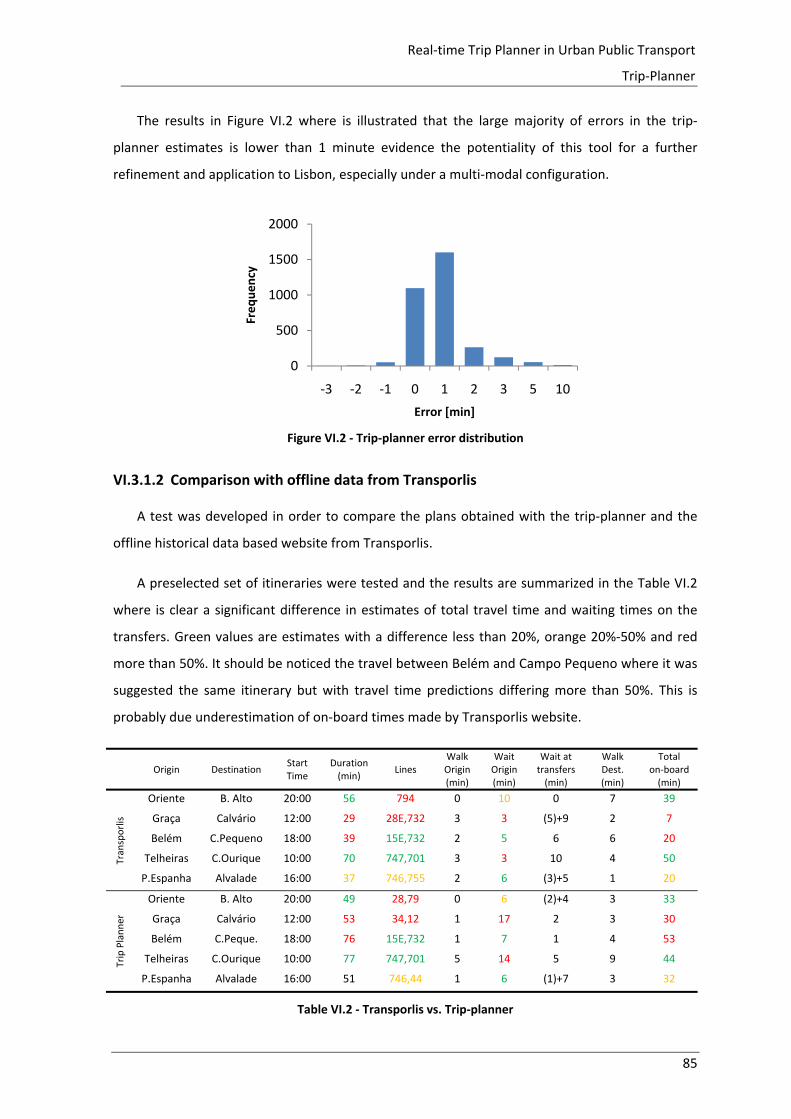
85


Trip‐Planner

The results in Figure VI.2 where is illustrated that the large majority of errors in the trip‐

planner estimates is lower than 1 minute evidence the potentiality of this tool for a further

refinement and application to Lisbon, especially under a multi‐modal configuration.

Figure VI.2 ‐ Trip‐planner error distribution

VI.3.1.2 Comparison with offline data from Transporlis

A test was developed in order to compare the plans obtained with the trip‐planner and the

offline historical data based website from Transporlis.

A preselected set of itineraries were tested and the results are summarized in the Table VI.2

where is clear a significant difference in estimates of total travel time and waiting times on the

transfers. Green values are estimates with a difference less than 20%, orange 20%‐50% and red

more than 50%. It should be noticed the travel between Belém and Campo Pequeno where it was

suggested the same itinerary but with travel time predictions differing more than 50%. This is

probably due underestimation of on‐board times made by Transporlis website.

Origin Destination

Start Time

Duration (min)

Lines Walk Origin (min)

Wait Origin (min)

Wait at transfers (min)

Walk Dest. (min)

Totalon‐board (min)

Transporlis

Oriente B. Alto 20:00 56 794 0 10 0 7 39

Graça Calvário 12:00 29 28E,732 3 3 (5)+9 2 7

Belém C.Pequeno 18:00 39 15E,732 2 5 6 6 20

Telheiras C.Ourique 10:00 70 747,701 3 3 10 4 50

P.Espanha Alvalade 16:00 37 746,755 2 6 (3)+5 1 20

Trip Planner

Oriente B. Alto 20:00 49 28,79 0 6 (2)+4 3 33

Graça Calvário 12:00 53 34,12 1 17 2 3 30

Belém C.Peque. 18:00 76 15E,732 1 7 1 4 53

Telheiras C.Ourique 10:00 77 747,701 5 14 5 9 44

P.Espanha Alvalade 16:00 51 746,44 1 6 (1)+7 3 32

Table VI.2 ‐ Transporlis vs. Trip‐planner

0

500

1000

1500

2000

‐3 ‐2 ‐1 0 1 2 3 5 10

Frequency

Error [min]

86


Trip‐Planner

VI.4 Conclusions

This Chapter presented a formulation of a new trip‐planner for the city of Lisbon, starting by

its conceptualization and the identification of the methodological tools required for its

deployment.

The introduction of Dijkstra schedule based algorithm was the key element for the

development of this tool, incorporating a utility based function to compute shortest paths.

The tests performed to a simple case study with the 19 locations, considering fixed

parameters for the user specification, showed the potentiality of the presented tool by measuring

an excellent overall fit between the observed and the estimated travel times and compliances at

boarding points.

87


Conclusions and Future Developments

VII Conclusions and Future Developments

This study presents the formulation of an ambitious Trip‐Planner tool for the bus and tram

system of the city of Lisbon. An extensive review showed that this type of real‐time application of

travel time predictions is not already available in large cities around the world that present very

complex and multimodal public transport systems.

This work represents a first step on the development of this tool with the development of a

complex simulation tool that allows testing the proposed real‐time information and prediction

system, and an innovative rule‐based decision model to calibrate and recalibrate speed and travel

time estimates for a 30 minutes time window.

The definition of the data mining process to analyze the available data and to create input

information for the prediction model, proved to be a decisive step in the development of a tool of

this kind. The spatial and speed configuration of the different services operated showed that

there are some operational patterns of the system that are similar even in very distant streets.

The obtained speed profiles distinguished types of Lisbon corridors that allow a more efficient and

steady operation, while other present a very slow and unstable one. This analysis may be relevant

to support future interventions on the network redesign from Carris, in order to optimize the

efficiency of their operation and increase the reliability on the deployed services from a users’

perspective.

The spatial distance between consecutives bus or tram stops in the Lisbon’s system also

revealed some problems in terms of equitable distribution to ensure a reasonable commercial

speed of the services, which otherwise are forced to stop immediately after the acceleration from

the previous stop, apart from the regular traffic constrains. This fact leads to a very low

commercial speed average speed registered by Carris in the year 2009 (14 km/h), which may limit

sufficiently their level of service and divert current users when in presence of a faster and more

reliable alternative. A striking fact that was observed with this analysis was the identification the

corridors with bus lanes do not present significantly higher commercial speeds than other regular

streets of the network.

The classified and processed data was then included in a comprehensive simulation model

using an Agent‐based formulation. This simulation tool aims to recreate the real system operation

in a computer based scenario, allowing the construction of different operation settings, as well as

88



road network behaviors that can affect the services operation. This artificial laboratory permitted

the development of an agents’ interaction environment and the central control of a speed and

travel time and forecast model.

The prediction model was built upon data linking different bus stops aggregated into groups,

instead of individual roads of the city network. In order to conciliate the estimates between

services operation corridors partially overlapped, it was created a new concept of Common

Section, which merged information from all the traversing sections to adjust the speeds of

vehicles within the same streets.

The prediction model was formulated in a rule‐based approach with four possible triggering

solutions depending on the accuracy of the estimates from the previous period: not change the

prediction model; calibrate a multivariate regression, produce a slight correction to the

multivariate regression estimates, or create a build‐up function for delay in sections, when a

incident is detected.

The obtained results from the model are very positive when compared both with a synthetic

speed model and with a log‐file from a real day. The hypotheses that may still limit the accuracy

of the model are the low number of registers, in the short term, of bus passages, which

significantly limits and bias the regression model. Furthermore, the unit of analysis, not directly

comparable to the one registered in the log file may also be a constraint to the ability to predict

precisely the travel times. Without these limitations it is expected to have even better results.

Finally, after the design and programming of the ABM simulation, the Trip‐Planner tool was

introduced by discussing the concepts behind this service, its objectives and the main potential

features. A small test‐bed example was then conduced to prove the value‐added of this new

formulation. For that purpose, a small set of notable points in the city were selected to assess

their possible connections at different hours of the day, but with the same user attributes

specification for the Dijkstra parameters (waking speed and willingness to accept an extra

transfer).

The results show, for an experimental run with a synthetic day of Carris operation a very good

fit and reliability of the retrieved queries that led to 86% of the error estimates lower than 1

minute and 95% lower than 2 minutes and to a correlation coefficient between estimates and real

travel times of 0.99.

89



The obtained results are very promising, although a larger and more complex test to the

model is required. Nonetheless, the information already retrieved by the model as well as the

speed of computation of all the possible solutions, shows the great potential of this application

for a future real world application in the city of Lisbon or in other cities around the world.

Although this dissertation deals already with some of the relevant issues of the development

of a tool of this kind, there still are a large set of questions to be solved and procedures to be

improved prior a real world deployment of the system.

One of the key questions that remain unanswered is the impact that a system like this may

have on the perception of users or potential users. Does the introduction of this system create the

momentum for a possible modal alternation of some private car users to the public transport

system? Is really information one of the triggers in the equation of mode selection or just a

necessary condition but not sufficient?

From a methodological point of view, are the formulations and algorithms selected the best

options for the set goals of the Travel‐planner? Is the rule‐based approach for different types of

network conditions or uncertainty appropriate?

The prediction model was designed to predict travel times for a time window of one hour in

advance. In a further iteration of this model, it is likely, with a richer historical database, with the

speed profiles categorized by day of the week and different seasons of the year to improve the fit

of the models the observed data. The development of more refined computation algorithms, to

get the projection window enlarged into a few hours may also be a focus for future research.

This study was based exclusively in Carris operational network, it would be desirable to

include in future iterations of the model different transport modes (e.g. subway, taxis, etc.).

Due to the short execution period to complete this study, there was not enough time to

extensively test the methodologies and refine the regressions computation. Therefore a new set

of tests is proposed and a future sensitive analysis to analyze how the predictions evolve with

different sets of historical and recent travel time measurements.

In the model developed, the historical data remained static which may restrict the horizon of

applicability of the model. It should be evaluated how historical data could be updated with

information regarding new travel time measurements using a Bayesian Statistical Inference

procedure.

90



This tool has the potential to be customizable by declaration of the users’ preferences (for

instance minimize transfers even if trip duration is increased by no more than 10 minutes), on the

basis of which the small set of suggestions would be ranked by decreasing order of preference.

91

Real-time Trip Planner in Urban Public Transport

References

References

Afandizadeh, S. and J. Kianfar (2009). A Hybrid Neuro-Genetic Approach to Short-Term Traffic Volume Prediction. International Journal of Civil Engineering Vol.7, No.1, pp. 41-48.

Arantes, A. and R. C. Marques (2009). Gestão e Teoria da Decisão - Course Material. Instituto Superior Técnico.

Banister, D. (2008). The sustainable mobility paradigm. Transport Policy Vol.15, No.2, pp. 73-80. Barbehenn, M. (1998). A Note on the Complexity of Dijkstra's Algorithm for Graphs with Weighted Vertices.

IEEE Trans. Comput. Vol.47, No.2, pp. 263. Barreto, J. M. (2002). Indrodução às Redes Neurais Artificiais. Barros, J. X. (2004). Urban Growth in Latin American Cities - Exploring urban dynamics through agent-based

simulation. Doctor of Philosophy, Bartlett School of Architecture and Planning, University College London, Place. 285.

Basu, J. K., D. Bhattacharyya and T.-h. Kim (2010). Use of Artificial Neural Network in Pattern Recognition. International Journal of Software Engineering and Its Applications Vol.4, No.2.

Battelle (2002). White paper on literature review of Real-time transit information systems. Beirao, G. and J. A. S. Cabral (2007). Understanding attitudes towards public transport and private car: A

qualitative study. Transport Policy Vol.14, No.6, pp. 478-489. Brueckner, J. K. (2001). Urban Sprawl: Lessons from Urban Economics. Brookings-Wharton Papers on Urban

Affairs, pp. 65-97. Carris. (2010). Indicadores de Actividade. Retrieved August 25, 2011, from

<http://www.carris.pt/pt/governo-societario/>. Cervero, R. (2009). Transport Infrastructure and Global Competitiveness: Balancing Mobility and Livability.

Annals of the American Academy of Political and Social Science Vol.626, pp. 210-225. Cervero, R., S. Murphy, C. Ferrell, N. Goguts, T. Yu-Hsin, A. G. B., B. John, J. Smith-Heimer, R. Golem, P.

Peninger, E. Nakajima, E. Chui, R. Dunphy, M. Myers, S. Mckay and N. Witenstein (2004). Transit-Oriented Development in the United States: Experiences, Challenges, and Prospects. TCRP Report 102. Transit Cooperative Research Program - The Federal Transit Administration, Washington D.C.

Clifton, C. (2011). data mining. Retrieved August 16, 2011, from <http://www.britannica.com/EBchecked/topic/1056150/data-mining>.

Cortez, P. and J. Neves (2000). Redes Neuronais ArtificiaisDepartamento de Informática, Escola de Engenharia Universidade do Minho, Place. 52.

De Ville, B. (2006). Decision trees for business intelligence and data mining using SAS Enterprise Miner. SAS Institute: Cary, N.C.

European Comission (2011). White paper on transport : roadmap to a single European transport area : towards a competitive and resource-efficient transport system. pp. 28 p. : col. ill. ; 30 cm.

Everitt, B., S. Landau and M. Leese (2001). Cluster analysis: Arnold. Fonseca, J. M. M. R. (1994). Indução de Árvores de Decisão, HistClass - Proposta de um algoritmo não

paramétricoDepartamento de Informática, Universidade Nova de Lisboa, Faculdade de Ciências e Tecnologia.

Fu, L. (1994). Neural networks in computer intelligence. New York ; London: McGraw-Hill. Gajewski, B. J. and L. R. Rilett (2005). Estimating Link Travel Time Correlation: An Application of Bayesian

Smoothing Splines. Journal of Transportation and Statistics Vol.7, No.2/3, pp. 53-70. Gelman, A. (2003). A Bayesian formulation of exploratory data analysis and goodness-of-fit testing.

International Statistical Review Vol.71, No.2, pp. 369-382. Heaton, J. (2005). Introduction to neural networks with Java. St. Louis: Heaton Research. Henley, D. H., I. P. Levin, J. J. Louviere and R. J. Meyer (1981). Changes in Perceived Travel Cost and Time for

the Work Trip during a Period of Increasing Gasoline Costs. Transportation Vol.10, No.1, pp. 23-34. Herrero, L. M. J. (2011). Transport and mobility: the keys to sustainability. Lychnos. Hu, M. Y., G. Q. Zhang and B. E. Patuwo (1998). Forecasting with artificial neural networks: The state of the

art. International Journal of Forecasting Vol.14, No.1, pp. 35-62. Human Resources Software. (2007). Interactive Voice Response. Retrieved August 21, 2011, from

<http://www.hr-software.net/pages/216.htm>.

http://www.carris.pt/pt/governo-societario/%3e

http://www.britannica.com/EBchecked/topic/1056150/data-mining%3e

http://www.hr-software.net/pages/216.htm%3e

92


References

IBM. (2011). Smarter Traffic. Retrieved July 29, 2011, from <http://www.ibm.com/smarterplanet/traffic>. IMTT (2006). Estudo Sobre as Condições de Exploração de Transportes em Táxi na Cidade de Lisboa.

Instituto da Mobilidade e dos Transportes Terrestres I.P. INE. (2011). Census 2011 - Resultados Preliminares. Retrieved September 3, 2011, from

<http://www.ine.pt/scripts/flex_v10/Main.html>. Ishak, S. and C. Alecsandru (2004). Optimizing traffic prediction performance of neural networks under

various topological, input, and traffic condition settings. Journal of Transportation Engineering-Asce Vol.130, No.4, pp. 452-465.

Kaufman, L. and P. J. Rousseeuw (2005). Finding groups in data: an introduction to cluster analysis: Wiley. Kenworthy, J., F. Laube, P. C. Newman and d. automobile (1999). An international sourcebook of automobile

dependence in cities, 1960-1990. Niwot, Colo.: University Press of Colorado. Ketchen, D. J. and C. L. Shook (1996). The application of cluster analysis in strategic management research

an analysis and critique. Strategic Management Journal Vol.17, No.6, pp. 441-458. Klakhaeng, N., J. Yaothanee, S. Sinthupinyo and W. Pattara-Atikom (2011). Traffic prediction models for

Bangkok traffic data. Electrical Engineering/Electronics, Computer, Telecommunications and Information Technology (ECTI-CON), 2011 8th International Conference on, 17-19 May 2011.

Lyons, G. and R. Harman (2002). The UK public transport industry and provision of multi-modal traveller information. International Journal of Transport Management Vol.1, pp. 1-13.

Macal, C. M. and M. J. North (2006). Tutorial on agent-based modeling and simulation part 2: How to model with agents. Proceedings of the 2006 Winter Simulation Conference, Vols 1-5, pp. 73-83

2307. Malek, A. (2008). Applications of Recurrent Neural Networks to Optimization Problems. Recurrent Neural

Networks. (X. H. a. P. Balasubramaniam, Eds.). Wien: I-Tech. Martínez, L. M. (2010). Activities, transportation networks and land prices as the key factors of location

choices: an agent-based model for the Lisbon Metropolitan Area (LMA). 12th

World Conference on Transport Research, Lisbon.

Martínez, L. M., G. Correia and J. M. Viegas (2011). An agent-based simulation procedure for measuring the market potential of shared taxis: an application to the Lisbon municipality. 90th Transport Research Board Annual Meeting, Washington D.C.

Merrifield, T. (2004). Heuristic Route Search in Public Transportation Networks, Ohio University. Min, W. (2007). Statistics researchers predict road traffic conditions. Retrieved August 16, 2011, from

<http://domino.watson.ibm.com/comm/research.nsf/pages/r.statistics.innovation.traffic.html>. ML. (2011). Mapa da rede. Retrieved August 28, 2011, from

<http://www.metrolisboa.pt/Default.aspx?tabid=138>. NextBus Inc. (2011). How Next Bus Works. Retrieved August 3, 2011, from <http://news.nextbus.com/>. Park, T. and S. Lee (2004). A Bayesian Approach for Estimating Link Travel Time on Urban Arterial Road

Network

Computational Science and Its Applications – ICCSA 2004. (A. Laganá, M. Gavrilovaet al, Eds.): Springer Berlin / Heidelberg. 3043: 1017-1025.

Quantum Inventions. (2009). Singapore Live Traffic. Retrieved October 6, 2011, from <http://www.livetraffic.sg/>.

Raphael, B. and I. F. C. Smith (2003). Fundamentals of computer-aided engineering: Wiley. Schweiger, C. L. and K. Shammout (2003). Strategies for improved traveler information. Washington, D.C.:

Transportation Research Board. Schweiger, C. L., A. United States. Federal Transit, P. Transit Cooperative Research, C. Transit Development

and B. National Research Council . Transportation Research (2003). Real-time bus arrival information systems. Washington, D.C.: Transportation Research Board.

Schwenker, F. and N. El Gayar (2010). Artificial neural networks in pattern recognition : 4th IAPT TC3 workshop, ANNPR 2010, Cairo, Egypt, April 11-13, 2010 : proceedings. Berlin: Springer.

Smith, J. Q. (2010). Bayesian decision analysis : principles and practice. Cambridge: Cambridge University Press.

Tang, T. (2010). Effects of the Spatial Distance between Two Adjacent Bus Stops on Traffic Flow. ASCE Conf. Proc. Vol.383, No.41123, pp. 36.

http://www.ibm.com/smarterplanet/traffic%3e

http://www.ine.pt/scripts/flex_v10/Main.html%3e

http://domino.watson.ibm.com/comm/research.nsf/pages/r.statistics.innovation.traffic.html%3e

http://www.metrolisboa.pt/Default.aspx?tabid=138%3e

http://news.nextbus.com/%3e

http://www.livetraffic.sg/%3e

93


References

Taylor, C., L. Nozick and A. Meyburg (1997). Selection and Evaluation of Travel Demand Management Measures. Transportation Research Record: Journal of the Transportation Research Board Vol.1598, No.-1, pp. 49-60.

TfL. (2011). iBus. Retrieved September 17, 2011, from <http://www.tfl.gov.uk/corporate/projectsandschemes/2373.aspx>.

U.S. Government. (2011). GPS Accuracy. Retrieved October 07, 2011, from <http://www.gps.gov/systems/gps/performance/accuracy/>.

Viegas, J. M. (2001). Making urban road pricing acceptable and effective: searching for quality and equity in urban mobility. Transport Policy Vol.8, No.4, pp. 289-294.

Viegas, J. M. (2010). Improving urban mobility through intermediate transport modes: the search for “double second-best” solutions. CESUR - Instituto Superior Técnico.

WHO (2007). Estimated deaths & DALYs attributable to selected environmental risk factors. World Health Organization.

Witten, I. H., E. Frank and M. A. Hall (2011). Data mining : practical machine learning tools and techniques. San Francisco, Calif. ; London: Morgan Kaufmann.

Wooldridge, M. (2002). Introduction to MultiAgent Systems: John Wiley & Sons. WSDT (2005). WSDOT 511 IVR Survey and Usability Testing Results. Washington State Department of

Transportation, Washington. WSDT and W. S. L. E. S. Publications (2004). Dynamic message signs: Washington State Dept. of

Transportation. Wynter, L. and W. M. Min, W. L. (2011). Real-time road traffic prediction with spatio-temporal correlations.

Transportation Research Part C-Emerging Technologies Vol.19, No.4, pp. 606-616. Zegras, P. C. and R. Gakenheimer (2006). Driving Forces in Developing Cities' Transportation Systems:

Insights from Selected Cases. Massachusetts Institute of Technology, Cambridge.

http://www.tfl.gov.uk/corporate/projectsandschemes/2373.aspx%3e

http://www.gps.gov/systems/gps/performance/accuracy/%3e

specifications and preliminary tests for lisbon · specifications and preliminary tests for lisbon...

Documents