spatiotemporal dynamics of a reaction-diffusion model of ... · a reaction-diffusion model is...

Journal of Mathematical Biology (2019) 79:1319–1355https://doi.org/10.1007/s00285-019-01396-7 Mathematical Biology

Spatiotemporal dynamics of a reaction-diffusion modelof pollen tube tip growth

Chenwei Tian1 ·Qingyan Shi2,3 · Xinping Cui1 · Jingzhe Guo4 ·Zhenbiao Yang4 · Junping Shi2

Received: 21 July 2018 / Revised: 6 June 2019 / Published online: 6 July 2019© Springer-Verlag GmbH Germany, part of Springer Nature 2019

AbstractA reaction-diffusion model is proposed to describe the mechanisms underlying thespatial distributions of ROP1 and calcium on the pollen tube tip. The model assumesthat the plasma membrane ROP1 activates itself through positive feedback loop, whilethe cytosolic calcium ions inhibit ROP1 via a negative feedback loop. Furthermore itis proposed that lateral movement of molecules on the plasma membrane are depictedby diffusion. It is shown that bistable or oscillatory dynamics could exist even in thenon-spatial model, and stationary and oscillatory spatiotemporal patterns are found inthe full spatial model which resemble the experimental data of pollen tube tip growth.

Keywords Pollen tube tip growth · Reaction-diffusion model · Oscillation ·Spatiotemporal patterns

Mathematics Subject Classification 92C15 · 92C80 · 35K57 · 35B36 · 35B32

XP Cui is partially supported by National Science Foundation Grant ATD-1222718 and the University ofCalifornia, Riverside AES-CE RSAP A01869; ZB Yang is partially supported by National Institute ofGeneral Medical Sciences Grant GM100130; JP Shi is partially supported by National ScienceFoundation Grant DMS-1715651; QY Shi is partially supported by China Scholarship Council.

B Junping [email protected]

1 Department of Statistics, University of California, Riverside, CA 92521, USA

2 Department of Mathematics, College of William and Mary, Williamsburg, VA 23187-8795, USA

3 School of Mathematical Sciences, Tongji University, Shanghai 200092, China

4 Department of Botany and Plant Sciences, Center for Plant Cell Biology, University of California,Riverside, CA 92521, USA

123

http://crossmark.crossref.org/dialog/?doi=10.1007/s00285-019-01396-7&domain=pdf

http://orcid.org/0000-0003-2521-9378

1320 C. Tian et al.

1 Introduction

Cell polarity is a fundamental feature of almost all cells. It is required for the differentia-tion of new cells, the formation of cell shapes, and cellmigration, etc (Edelstein-Keshetet al. 2013; Mogilner et al. 2012). Polar tip growth is a specialized form of cell growth,in which growth is limited to the single end of the cell, allowing the cell to rapidlyelongate and penetrate tissues. Pollen tubes provide an excellent model for studying tipgrowth and spatiotemporal oscillation, such asCa2+ oscillation (Feijó et al. 2001). Asthe male structure carrying sperm cells, pollen tubes protrude from pollen grains, andelongate by extremely polarized cell growth known as tip growth. They pass throughseveral female tissues to reach the ovule, in which the sperm cells are released fromthe pollen tube and fuse with the egg cell and the central cell to grow an embryo andendosperm. To efficiently target to the ovule, pollen tubes grow extraordinarily fast inan oscillatory fashionwhich is controlled by theRhoGTPase (ROP1)molecular switch(Li et al. 1999;Yang 2008).Within the signaling network regulating polarized exocyto-sis to the tip of pollen tube, plasma membrane localized ROP1 at the pollen tube apexis regulated by positive and negative feedback loops through exocytosis. Polarizedexocytosis regulated by active ROP1 couple with ROP1 signaling to the compositionand mechanics of the cell wall (Luo et al. 2017). The resulting asymmetric cell wallstructure determines the strain rates and thereby the geometry of the cell wall. To pro-mote polar exocytosis, the ROP1 signaling network is localized dynamically to the tipplasma membrane as an apical cap, whose shape changes in an oscillatory manner asgrowth oscillation. Therefore, modeling the oscillatory dynamic of ROP1 distributionon the plasma membrane is the key to understand the tip growth of pollen tube.

As a key regulator of the self-organizing pollen tube system, the activity and distri-bution of ROP1 are fine-tuned by both positive and negative feedback mechanisms aswell as slow diffusion. It has been indicated that the Ca2+ is involved in the negativefeedback regulation of ROP1. In addition, it also has been shown that ROP1 promotesthe formation of the intracellular Ca2+ gradients probably via the influx of extracel-lular Ca2+ (Gu et al. 2005; Li et al. 1999). In recent work (Luo et al. 2017; Xiao et al.2016), the Yang and Cui group demonstrated that spatial distribution of active ROP1 asan apical cap can be achieved through both positive and negative feedbacks, and a gra-dient of guidance signal can promote ROP1 activation and lead to an asymmetric dis-tribution of active ROP1 and result in the change of growth direction. All of these priorfindings provide us the basis to uncover the quantitative principles behind the formationand regulation of rapid spatiotemporal oscillation of ROP1-Ca2+ signaling networkand their linkage to growth redirection. In this paper, we propose a reaction-diffusionmodel of ROP1 and Ca2+ distributions on the cell plasma membrane to show howROP1 and Ca2+ are spatiotemporally intertwined and what are the quantitative rela-tionship between them in order to generate theROP1-Ca2+ spatiotemporal oscillation.

A PDE model for yeast cell polarization was proposed in Altschuler et al. (2008)but it only considered the positive feedback. The reaction-diffusion pattern formationtheory suggests that positive feedback alone cannot generate stable spatial patterns.Reaction-diffusion models for yeast cell polarization induced by pheromone spatialgradient have been established by Chou et al. (2008), Lo et al. (2014), Moore et al.(2008), Yi et al. (2007) and Zheng et al. (2011), see also (Goryachev and Pokhilko

123

Spatiotemporal dynamics of a reaction-diffusion model... 1321

2008; Holmes and Edelstein-Keshet 2016; Jilkine et al. 2007; Mori et al. 2011; Rätzand Röger 2012). In the recent work (Xiao et al. 2016), a PDE model for the ROP1dynamics for the pollen tube tip growth was proposed:

⎧⎨

⎩

Rt=kp f Rα

(

Rtot−∫ L

−LR(s, ·)ds

)

−kn f R+DRRss, (s, t) ∈ (−L, L) × [0, T ],Rs(−L, t) = Rs(L, t) = 0, t ∈ [0, T ].

(1.1)

It is shown by Xiao et al. (2016) that the positive steady state of (1.1) is uniqueand has a soliton-like profile which resembles the Arabidopsis PT experimental ROP1data obtained in Yang lab. Moreover the parameters kp f and kn f were estimated basedon the numerically integrated steady state profile of (1.1) and the experimental datausing a constrained Least Squares (CNLS) method. The experimental data fits withthe numerical steady state of (1.1) reasonably well. However the positive steady stateof (1.1) indeed is unstable with respect to the time-evolution dynamics of (1.1), whichsuggests that some other feedback mechanism or other key activator/inhibitor in thesystem is not identified in (1.1). Also the model (1.1) cannot produce time-periodicpatterns which occurs in the pollen tube growth.

Reaction-diffusion systems have been widely used in developmental biology mod-eling since the pioneer work of Turing (1952), see for example Gierer and Meinhardt(1972),Kondo andMiura (2010) and Maini et al. (1997). Rigorous bifurcation analysisfor a wide range of reaction-diffusionmodels has been done in recent years (Chen et al.2014; Jin et al. 2013;Wanget al. 2011, 2016;Yi et al. 2009;Zhou andShi 2015), and thegeneration of spatially non-homogeneous time-periodic patterns in reaction-diffusionmodels with time delay has been considered by Busenberg and Huang (1996), Chenet al. (2013, 2018), Chen and Yu (2016a, b), Chen and Shi (2012), Guo (2015), SeirinLee et al. (2011), Shi et al. (2017, 2019b), Su et al. (2009), Yan and Li (2010) and Yiet al. (2017).

Our proposed model in this paper couples the spatial Ca2+ dynamics with theROP1 dynamics in (1.1). It is based on the ROP1 dynamics described in (1.1), butadds the associated Ca2+ dynamics which forms a reaction-diffusion model withan activator-inhibitor pair, nonlocal and time-delay effect (see Sect. 2). The base-line kinetic model is a system of two ordinary differential equations with intriguingdynamics: (i) bistability; (ii) limit cycles generated through Hopf bifurcations; (iii)degenerate trivial steady state (0, 0). A detailed analysis and classification is given forthe kinetic system in Sect. 3. In Sect. 4, the analysis and simulation of the reaction-diffusion system is given. It is demonstrated that a rich spectrum of spatiotemporalpatterns can be produced by our proposed model: non-constant steady states, spatiallyhomogeneous time-periodic solutions, and various spatially nonhomogeneous time-periodic solutions. Of particular interest to the pollen tube tip growth is the spatiallynonhomogeneous time-periodic solutions, which predicts the ROP1-Ca2+ spatiotem-poral oscillation. Indeed our numerical finding in certain parameter range qualitativelymatches with experimental data generated in Yang Lab (Hwang et al. 2005), whichpartially validates the proposed reaction-diffusion model and underlying modelingprinciple. Some concluding remarks are given in Sect. 5.

123

1322 C. Tian et al.

Fig. 1 ROP1 and Ca2+ polarization dynamics. Left: ROP1 dynamics; Right: Ca2+ dynamics

2 Model

To model the cell-signaling process on the membrane, we simplify the cell membraneas a one-dimensional spatial domain x ∈ (−L, L), where x is the (signed) distancefrom the tip of the membrane x = 0. Note that for simplicity, we ignore the geometriccurvature of the membrane in the current model. The main variables in the models arethe active ROP1 concentration R(x, t) and the Calcium ion Ca2+ concentration at thelocation x and time t . Moreover, we set L to be large enough so that the ROP1 andCa2+ concentration gradients are close to zero on the boundary, so we assume that Rand C satisfy no-flux boundary condition:

∂R(x, t)

∂x= ∂C(x, t)

∂x= 0, x = −L, L. (2.1)

The redistribution of signaling molecules ROP1 is determined by the rates of fourfundamental transport mechanisms (Altschuler et al. 2008): (1) recruitment (k f b) ofcytoplasmic molecules to the locations of membrane-bound signaling molecules; (2)spontaneous association (kon) of cytoplasmic molecules to random locations on theplasma membrane; (3) lateral diffusion (D) of molecules along the membrane; and(4) random disassociation (kof f ) of signaling molecules from the membrane.

In our model, we eliminate the spontaneous term because the spontaneous ratekon is much smaller than k f b and kof f . Altschuler et al. (2008) proposed a stochasticmodel showing that no cluster will be formed if kon is not small, and then mostparticles will arrive on the membrane through spontaneous associations rather thanrecruitment. So we can assume that kon is small enough. Moreover, the time betweentwo spontaneous event follows an exponential distribution with expectation Ton =(kon(1 − heq)N )−1. When kon is small, Ton will be large which leads to a long timebetween two spontaneous events. Our partial differential equation model describesthe change of distribution of ROP1 intensity in a short period of time. Therefore, weeliminate the spontaneous term when we model the cell-signaling process.

In this case, the ROP1 polarization dynamics without spontaneous association canbe simplified as three main procedures (see Fig. 1 left panel): (1) activation of inactiveROP1; (2) inhibition of active ROP1; (3) lateral diffusion of molecules along themembrane. The activation of ROP1 can be considered as a positive feedback whilethe deactivation of ROP1 as a negative feedback. Both activation and inhibition ratesare proportional to substrate concentrations.

123


Fig. 2 Interaction diagram of ROP1 and Ca2+

The lateral movement of ROP1 is modeled by a diffusion term D1∂2R(x, t)

∂x2, where

D1 is the diffusion coefficient of ROP1. As for activation of ROP1, it is shown by biol-ogy model simulation, the activation rate is proportional to Rα where the exponentsatisfies 1 < α < 2. Moreover, since majority of inactive ROP1 are in cytoplasm withhigh mobility, the activation rate is proportional to the total amount of cytoplasmic

molecules (i.e. Rtotal −∫ L

−LR(x, t)dx) with rate kp f . On the other hand, most active

ROP1 are on the membrane. Since molecules on the membrane have much less mobil-ity, the inhibition rate is proportional to the density of molecules (i.e. R(x, t)) at anygiven location with rate kn f . Moreover, Ca2+ can inhibit ROP1 with some thresholdkh and an inhibition function

g(C) = C2

C2 + k2h. (2.2)

Here g(C) is a Hill function which shows a transition from low inhibition rate at lowCalcium density, and a high but bounded inhibition rate at a high Calcium density.The constant kh is the half-saturation value indicating the threshold between the lowand high Calcium density. Hence R(x, t) satisfies a reaction-diffusion equation witha nonlocal integral term:

∂R(x, t)

∂t= kp f R

α(x, t)

(

Rtotal −∫ L

−LR(x, t)dx

)

− kn f R(x, t)g(C(x, t)) + D1∂2R(x, t)

∂x2. (2.3)

On the other hand, we simplify the Ca2+ activities as following three procedures:(1) influx of Ca2+; (2) self-decay of Ca2+; and (3) diffusion of Ca2+ along the

membrane (see Fig. 1 right panel). The diffusion of Ca2+ is given by D2∂2C(x, t)

∂x2,

where D2 is the diffusion coefficient of Ca2+. The Ca2+ ions could flow into thecell through Calcium channel on the membrane, and the Ca2+ inflow is controlledby ROP1 with rate kac. Also there is a time delay τ in this promotion. In this work,we model Ca2+ promotion with kacR(x, t − τ) to show a linear response of Calciuminflux to the ROP1 density, which is supported by several studies from Yang lab(Hwang et al. 2005; Li et al. 1999; Yan et al. 2009). On the other hand, self-decay ofCa2+ is proportional to substrate concentration at a certain rate kdc. Therefore, the

123

1324 C. Tian et al.

Ca2+ activities are described by a reaction-diffusion equation with time-delay:

∂C(x, t)

∂t= kacR(x, t − τ) − kdcC(x, t) + D2

∂2C(x, t)

∂x2. (2.4)

Note that ROP1 activates both ROP1 andCa2+ growth, andCa2+ inhibits both ROP1and Ca2+ (see Fig. 2).

Now summarizing the above description, adding the proper initial conditions, wehave the following full system for the interaction between the ROP1 and Ca2+ on thecell membrane:

⎧⎪⎪⎪⎪⎪⎪⎪⎪⎨

⎪⎪⎪⎪⎪⎪⎪⎪⎩

Rt = kp f Rα

(

Rtotal −∫ L

−LRdx

)

− kn fRC2

C2 + k2h+ D1Rxx , (x, t) ∈ (−L, L) × (0, T ),

Ct = kac R(x, t − τ) − kdcC + D2Cxx , (x, t) ∈ (−L, L) × (0, T ),

Rx (x, t) = Cx (x, t) = 0, x = −L, L,

R(x, t) = R0(x, t), (x, t) ∈ (−L, L)×[−τ, 0],C(x, 0) = C0(x), x ∈ (−L, L).

(2.5)Here Rt , Ct , Rxx , Cxx are abbreviated notations for partial derivatives, and

R = R(x, t), C = C(x, t) except the term with time delay.To reduce the number of parameters in the problem and convert the equation into

a dimensionless form, we introduce the normalized quantities:

t̃ = kdct, x̃ =√kdcD2

x, R̃ = 2LR

Rtotal, C̃ = 2LkdcC

Rtotalkac, (2.6)

k1 = 2Lkp fkdc

(Rtotal

2L

)α

, k2 = kn f2Lkp f

(2L

Rtotal

)α

, k3 = 2Lkhkdckac Rtotal

, D = D1

D2,

(2.7)

τ̃ = kdcτ, L̃ = L

√kdcD2

, T̃ = kdcT . (2.8)

With these normalized quantities, the PDEmodel (2.5) is rewritten in the followingnormalized form:

⎧⎪⎪⎪⎪⎪⎪⎪⎪⎨

⎪⎪⎪⎪⎪⎪⎪⎪⎩

R̃t̃ = k1 R̃α

(

1 − 1

2L̃

∫ L̃

−L̃R̃d x̃

)

− k1k2R̃C̃2

C̃2 + k23+ DR̃x̃ x̃ , (x̃, t̃) ∈ (−L̃, L̃) × (0, T̃ ),

C̃t̃ = R̃(x̃, t̃ − τ̃ ) − C̃ + C̃x̃ x̃ , (x̃, t̃) ∈ (−L̃, L̃) × (0, T̃ ),

R̃x̃ (x̃, t̃) = C̃x̃ (x̃, t̃) = 0, x̃ = −L̃, L̃,

R̃(x̃, t̃) = R̃0(x̃, t̃), (x̃, t̃) ∈ (−L̃, L̃) × [−τ̃ , 0],C̃(x̃, 0) = C̃0(x̃), x̃ ∈ (−L̃, L̃).

(2.9)

123


Dropping the ∼ in (2.9), we have the system

⎧⎪⎪⎪⎪⎪⎪⎪⎪⎨

⎪⎪⎪⎪⎪⎪⎪⎪⎩

Rt = k1Rα

(

1 − 1

2L

∫ L

−LRdx

)

− k1k2RC2

C2 + k23+ DRxx , (x, t) ∈ (−L, L) × (0, T ),

Ct = R(x, t − τ) − C + Cxx , (x, t) ∈ (−L, L) × (0, T ),

Rx (x, t) = Cx (x, t) = 0, x = −L, L,

R(x, t) = R0(x, t), (x, t) ∈ (−L, L) × [−τ, 0],C(x, 0) = C0(x), x ∈ (−L, L).

(2.10)From now on, we will analyze the dynamics behavior of the simplified system

(2.10). Indeed, in this paper, we will only consider the case that τ = 0 to show therich dynamics of corresponding ODE and PDE models, and the effect of delay willbe considered in a future work.

3 Non-spatial dynamics

In system (2.10), if the initial conditions (R0(x, t),C0(x)) are spatially homogeneousand τ = 0, then the corresponding solution of (2.10) is also spatially homogeneousand it satisfies ⎧

⎪⎨

⎪⎩

Rt = k1Rα(1 − R) − k1k2RC2

C2 + k23,

Ct = R − C .

(3.1)

The steady states of (3.1) satisfy

⎧⎪⎨

⎪⎩

k1Rα(1 − R) − k1k2RC2

C2 + k23= 0,

R − C = 0.(3.2)

A nonnegative steady state is either the trivial one (R,C) = (0, 0), or a positive onesatisfying

Rα−1(1 − R) − k2C2

C2 + k23= 0, C = R. (3.3)

Then (3.3) is equivalent to C = R and

f (R) ≡ k2 − Rα−3(1 − R)(R2 + k23) = 0. (3.4)

The following result shows the existence and exact multiplicity of roots R of (3.4),which also reveals the existence and exact multiplicity of steady states of (3.1) in form(R, R).

Proposition 3.1 There exists a constant k31 > 0 such that

1. If 0 < k3 < k31, then there exists 0 < k21 < k22 which depend on k3 and α suchthat

123

1326 C. Tian et al.

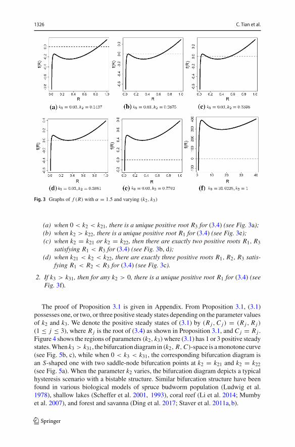
Fig. 3 Graphs of f (R) with α = 1.5 and varying (k2, k3)

(a) when 0 < k2 < k21, there is a unique positive root R3 for (3.4) (see Fig. 3a);(b) when k2 > k22, there is a unique positive root R1 for (3.4) (see Fig. 3e);(c) when k2 = k21 or k2 = k22, then there are exactly two positive roots R1, R3

satisfying R1 < R3 for (3.4) (see Fig. 3b, d);(d) when k21 < k2 < k22, there are exactly three positive roots R1, R2, R3 satis-

fying R1 < R2 < R3 for (3.4) (see Fig. 3c).

2. If k3 > k31, then for any k2 > 0, there is a unique positive root R1 for (3.4) (seeFig. 3f).

The proof of Proposition 3.1 is given in Appendix. From Proposition 3.1, (3.1)possesses one, or two, or three positive steady states depending on the parameter valuesof k2 and k3. We denote the positive steady states of (3.1) by (R j ,C j ) = (R j , R j )

(1 ≤ j ≤ 3), where R j is the root of (3.4) as shown in Proposition 3.1, and C j = R j .Figure 4 shows the regions of parameters (k2, k3)where (3.1) has 1 or 3 positive steadystates.When k3 > k31, the bifurcation diagram in (k2, R,C)-space is amonotone curve(see Fig. 5b, c), while when 0 < k3 < k31, the corresponding bifurcation diagram isan S-shaped one with two saddle-node bifurcation points at k2 = k21 and k2 = k22(see Fig. 5a). When the parameter k2 varies, the bifurcation diagram depicts a typicalhysteresis scenario with a bistable structure. Similar bifurcation structure have beenfound in various biological models of spruce budworm population (Ludwig et al.1978), shallow lakes (Scheffer et al. 2001, 1993), coral reef (Li et al. 2014; Mumbyet al. 2007), and forest and savanna (Ding et al. 2017; Staver et al. 2011a, b).

123


Fig. 4 The number of positive steady states of system (3.1) for different values of (k2, k3) with α = 1.5.Here the horizontal axis is k3 and vertical axis is k2

Fig. 5 Bifurcation diagrams of system (3.1) with α = 1.5

Nextwe consider the local stability of the steady states (0, 0) and (R j , R j ) (1 ≤ j ≤3) with respect to (3.1). First at steady state (0, 0), the Jacobian matrix is

(0 01 −1

)

.

Therefore we have two eigenvalues λ1 = 0 and λ2 = −1 < 0 which indicatesthat (0, 0) is a degenerate steady state. One can apply the theory of two-dimensionaldynamical system to obtain the following description of the dynamics of (3.1) near(0, 0):

Proposition 3.2 For any k1, k2, k3 > 0, there exists a δ > 0 such that in the neighbor-hood B = {(R,C) : 0 < R < δ, 0 < C < δ} of (0, 0),1. (3.1) has a unique center manifold Wc = {(R, hc(R)) : 0 ≤ R < δ} for (3.1) such

that hc(0) = 0 and h′c(0) = 1, and the orbit of (3.1) on Wc is unstable;

123

1328 C. Tian et al.

Fig. 6 Dynamical behavior of (3.1) near (0, 0). Here α = 1.5, k1 = 175, k2 = 0.31, k3 = 0.0316, and theinitial conditions for the solution orbits in the right panel are (R(0),C(0)) = (0.05, 0.05) and (0.04, 0.04)

2. there exists a function hs : (0, δ) → (0, δ) such that the region O = {(R,C) :0 ≤ R ≤ hs(C), 0 < C < δ} is invariant, and for any (R0,C0) ∈ O, the solution(R(t),C(t)) of (3.1) with (R(0),C(0)) = (R0,C0) satisfies lim

t→∞(R(t),C(t)) =(0, 0).

3. other orbits in B exhibit saddle behavior near (0, 0), that is, the orbit does notapproach (0, 0) as t → ∞ or t → −∞, and for t > T , the orbit leaves theneighborhood B.

The proof of Proposition 3.2 is given in Appendix. It shows that there is a “horn”-shaped region belonging to the basin of attraction of the origin (0, 0). Indeed forany parameter values, if the initial value of Ca2+ C0 is sufficiently large, then thesolution will converge to (0, 0) (see Fig. 6). So our subsequent discussion will be forthe remaining part of the phase portrait in which the orbits do not converge to (0, 0).

For positive steady states, we linearize (3.1) at a steady state (R j , R j ) ( j = 1, 2, 3),then we obtain the Jacobian matrix as

J (R j , R j ) =(k1R j f ′

1(R j ) −k1R j f ′2(R j )

1 −1

)

, (3.5)

where

f1(R) = Rα−1(1 − R), f2(R) = k2R2

R2 + k23. (3.6)

Hence we find that

Tr(J (R j , R j )) = k1R j f′1(R j ) − 1, (3.7)

Det(J (R j , R j )) = k1R j ( f′2(R j ) − f ′

1(R j )). (3.8)

We recall that a steady state (R, R) of (3.1) is a sink or spiral sink if both eigenvaluesof J (R, R) are of negative real parts; it is a source or spiral source if both eigenvaluesof J (R, R) are of positive real parts; and it is a saddle if J (R, R) has one positive and

123


one negative eigenvalue. From the trace-determinant theory, it is easy to know that(R, R) is a sink or spiral sink if Tr(J ) < 0 and Det(J ) > 0; it is a source or spiralsource if Tr(J ) > 0 and Det(J ) > 0; and it is a saddle if Tr(J ) ∈ R and Det(J ) < 0.

For our next result regarding the local stability of the positive steady state (R j , R j )

( j = 1, 2, 3) obtained above,wedetermine the stability using the trace anddeterminantof J (R,C).We also observe that the steady states of (3.1) are independent of parameterk1, but k1 does affect the stability of steady states. For fixed α ∈ (1, 2) and k3 > 0,and any 0 < R < 1, the pair (R, R) can be a steady state of (3.1) for exactly one valueof k2 > 0 by the relation (from (3.2)):

k2 = Rα−3(1 − R)(R2 + k23). (3.9)

That is, for fixed α ∈ (1, 2) and k3 > 0, the set of steady states of (3.1) can beparameterized by R as a bifurcation diagram (see Fig. 5):

� = {(k2(R), R, R) : R ∈ (0, 1)}, (3.10)

where k2(R) is given by (3.9). Now we state our results on the local stability of thepositive steady state in terms of parametrization in (3.10).

Theorem 3.3 Suppose that α ∈ (1, 2) and k3 > 0, and k2(R) is defined as in (3.9) sothat (R, R) is a positive steady state of (3.1) with k2 = k2(R) for 0 < R < 1.

1. If k3 > k31 (defined inProposition3.1), thenDet(J (R, R)) > 0 for any R ∈ (0, 1);and if 0 < k3 < k31, then there exist r1, r2 > 0 such that Det(J (R, R)) > 0 forR ∈ (0, r1) ∪ (r2, 1), and Det(J (R, R)) < 0 for R ∈ (r1, r2). Here k2(r1) = k21and k2(r2) = k22 (defined in Proposition 3.1).

2. Define

k11 = α2α−1

(α − 1)2α−1 . (3.11)

If 0 < k1 < k11, then Tr(J (R, R)) < 0 for any R ∈ (0, 1); and if k1 > k11, thenthere exist 0 < R̃1 < R̃2 such that Tr(J (R, R)) < 0 for R ∈ (0, R̃1) ∪ (R̃2, 1),and Tr(J (R, R)) > 0 for R ∈ (R̃1, R̃2).

According to Theorem 3.3, we can have following results for 0 < k3 < k31, whenthere are at least one and at most three positive steady state of (3.1):

1. The middle positive steady state (R2, R2) is always a saddle.2. The largest positive steady state (R3, R3) or the smallest one (R1, R1) is either a

sink or spiral sink, or a source or spiral source, but it is not a saddle.3. Define

Is = ((0, r1) ∪ (r2, 1)) ∩ ((0, R̃1) ∪ (R̃2, 1)). (3.12)

Then when R ∈ Is , the positive steady state (R, R) is a sink or spiral sink whichis locally asymptotically stable. In particular, when R > 0 is sufficiently small orwhen R is close to 1, then (R, R) is a sink or spiral sink.

123

1330 C. Tian et al.

4. DefineIu = ((0, r1) ∪ (r2, 1)) ∩ (R̃1, R̃2). (3.13)

Then when R ∈ Iu , the positive steady state (R, R) is a source or spiral sourcewhich is unstable.

The proof of Theorem 3.3 is in the Appendix. Note that the stable regime Is isalways not an empty set as it contains a right neighborhood of R = 0 and a leftneighborhood of R = 1, but Is may also contain another connected component whichis disconnected from R = 0 and R = 1. The unstable regime Iu could be empty, andthat happens when 0 < k1 < k11. However Iu is not empty when k1 is chosen assufficiently large. Indeed for fixed k3 > 0, one has that

limk1→∞ R̃1 = 0, lim

k1→∞ R̃2 = α − 1

α. (3.14)

The local stability analysis given in Theorem 3.3 can be used to guide our classifi-cation of global dynamics of (3.1). A complete classification in terms of parameters(k1, k2, k3) is rather exhaustive and it will not be given here. Here we focus on inwhich cases, the system (3.1) shows sustained temporal oscillations. The follow resultclassifies the occurrence of Hopf bifurcations in terms of parameters k1, k2 and k3.

Proposition 3.4 Suppose that α ∈ (1, 2), and define

g(R) = Rα−1[(α − 1) − αR]. (3.15)

Let k31, k11 be defined as in Proposition 3.1 and (3.11) respectively, and letr1, r2, R̃1, R̃2 > 0 be defined in Theorem 3.3. We also define k̃21 = k2(R̃1) andk̃22 = k2(R̃2).

1. If k3 > k31, (3.1) has a unique positive steady state for all k1, k2 > 0. Moreover

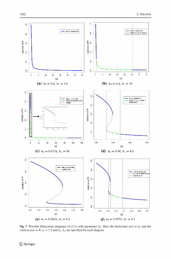
(a) When k1 < k11, the unique positive steady state of (3.1) is a sink or spiral sinkfor any k2 > 0. (see Fig. 7a)

(b) When k1 > k11, the unique positive steady state of (3.1) is a sink or spiralsink for k2 ∈ (0, k̃22) ∪ (k̃21,∞), and is unstable for k2 ∈ (k̃22, k̃21); Hopfbifurcations occur at k2 = k̃21 and k2 = k̃22, and there exists at least oneperiodic orbit for k2 ∈ (k̃22, k̃21). (see Fig. 7b)

2. If 0 < k3 < k31, (3.1) has at least one and at most three positive steady states, andwhen there exist three positive steady states, the middle one (R2, R2) is a saddle.Moreover

(c) If k1 > 1/g(r2), then Hopf bifurcations occur at k̃22 on the large steady state(R3, R3) and at k̃21 on the small steady state (R1, R1) of (3.1). (see Fig. 7c)

(d) If 1/g(r1) < k1 < 1/g(r2), then the large positive steady state (R3, R3) isalways a sink or spiral sink, and a Hopf bifurcation occurs at k̃21 on the smallpositive steady state (R1, R1) of (3.1). (see Fig. 7d)

123


(e) Define

k̃3 =√

(α − 1)5

α3(−α2 + 5α − 2). (3.16)

If 0 < k1 < 1/g(r1) and 0 < k3 < k̃3, or 0 < k1 < k11 and k̃3 < k3 < k31,then both the large positive steady state (R3, R3) and the small positive steadystate (R1, R1) are always sink or spiral sink, and there is no Hopf bifurcationoccurring. (see Fig. 7e)

(f) If k11 < k1 < 1/g(r1) and k̃3 < k3 < k31, then the large positive steady state(R3, R3) is always a sink or spiral sink, and Hopf bifurcations occur at k̃21and k̃22 on the small positive steady state (R1, R1) of (3.1). (see Fig. 7f)

The proof of Proposition 3.4 is in the Appendix. The six bifurcation diagramsof steady states and Hopf bifurcations are shown in Fig. 7, and a classification of(k3, k1) parameter regions in which Hopf bifurcations with parameter k2 can occur issummarized in Fig. 8.

Guided by bifurcation diagrams above, there are following six possible dynamicphase planes and dynamics of (R(t),C(t)) solutions. Note that from Proposition 3.2,there is always a region of initial conditions that orbits starting from there converge tothe origin (0, 0) as t → ∞. So in the following we only describe the dynamics belowthe basin of attraction of (0, 0).

1. There is only one positive steady state R1, which is a sink or spiral sink. All thesolutions will converge to R1. For example, when α = 1.5, k1 = 9.5, k2 = 1,k3 = 0.06, there is a spiral sink at R1 = 0.02587. (See Fig. 9 upper row)

2. There is only one positive steady state R1, which is a source or spiral source, andthere is a limit cycle around R1. For example, when α = 1.5, k1 = 15, k2 = 1,k3 = 0.06, there is a limit cycle around positive steady state R1 = 0.02587. (SeeFig. 9 lower row)

3. There are three positive steady states R1, R2 and R3; R2 is a saddle point whileR1 and R3 are sinks or spiral sinks. A solution will converge to either R1or R3depending on the initial value. For example, when α = 1.5, k1 = 5, k2 = 0.4035,k3 = 0.0707, there are two sinks R1 = 0.1418 and R3 = 0.3194. The solutionconverges to R1 = 0.1418 if the initial value is (R(0),C(0)) = (0.1, 0.4), whileto R3 = 0.3194 if (R(0),C(0)) = (0.4, 0.1). (See Fig. 10)

4. There are three positive steady states R1, which is a source, R2, which is a saddlepoint, R3, which is a sink. Here except the stablemanifold of R2, all other solutionsconverge to R3. For example, when α = 1.5, k1 = 12, k2 = 0.31, k3 = 0.0316,the sink R3 = 0.6013 attracts most of initial condition, and Fig. 11 shows an orbitconnecting R1 to R3. It is also possible that there is a limit cycle around R1, butthe parameter range for that case is not robust.

5. There are three positive steady states R1, R2 and R3. R2 is a saddle point whileR1 and R3 are source or spiral source. Again the parameter range supporting suchdynamics is not robust enough so we do not include a phase portrait for that casehere.

123

1332 C. Tian et al.

Fig. 7 Possible bifurcation diagrams of (3.1) with parameter k2. Here the horizontal axis is k2 and thevertical axis is R, α = 1.5 and k1, k3 are specified for each diagram

123


Fig. 8 Classification of (k3, k1) parameter region for Hopf Bifurcation occurrence with α = 1.5. Hereregions (a) to (f) represent (k3, k1) parameter regions of cases (a) to (f) in Proposition 3.4, respectively

Fig. 9 Dynamic behavior of (3.1). Here α = 1.5, k2 = 1, k3 = 0.06; Upper: k1 = 9.5; Lower: k1 = 15

123

1334 C. Tian et al.

Fig. 10 Dynamic behavior of (3.1). Here α = 1.5, k1 = 5, k2 = 0.4035, k3 = 0.0707

Fig. 11 Dynamic behavior of (3.1). Here α = 1.5, k1 = 12, k2 = 0.31, k3 = 0.0316

4 Spatial dynamics

In this section, we consider the dynamics of the reaction-diffusion model (2.10) whichis also with nonlocal term and delay. First we consider the model without the timedelay:

⎧⎪⎪⎪⎪⎪⎪⎪⎪⎨

⎪⎪⎪⎪⎪⎪⎪⎪⎩

Rt = DRxx + k1Rα

(

1 − 1

2L

∫ L

−LRdx

)

− k1k2RC2

C2 + k23, (x, t) ∈ (−L, L) × (0, T ),

Ct = Cxx + R − C, (x, t) ∈ (−L, L) × (0, T ),

Rx (x, t) = Cx (x, t) = 0, x = −L, L, t ∈ (0, T ),

R(x, t) = R0(x, t), (x, t) ∈ (−L, L) × [−τ, 0],C(x, 0) = C0(x), x ∈ (−L, L).

(4.1)We shall show that spatiotemporal pattern formation is possible for (4.1) as a com-

bined effect of diffusion, kinetic dynamics as shown in Sect. 3, and also the nonlocalintegral term.

123


It is easy to see that a steady state (R∗, R∗) of (3.1) is a constant steady statesolution of (4.1). Linearizing Eq. (4.1) at a constant steady state (R∗, R∗), we obtainthe following eigenvalue problem which determines the linear stability of the constantsteady state:

⎧⎪⎪⎪⎨

⎪⎪⎪⎩

μφ = Dφxx + (k1R∗ f ′

1(R∗) + k1Rα∗)φ − k1R∗ f ′

2(R∗)ψ − k1Rα∗1

2L

∫ L

−Lφdx, x ∈ (−L, L),

μψ = ψxx + φ − ψ, x ∈ (−L, L),

φx (x) = ψx (x) = 0, x = −L, L,

(4.2)where f1(R) and f2(R) are defined in (3.6). The eigenvalue problem (4.2) can beconsidered in the real-valued Sobolev space with the Neumann Boundary problemX = {(φ,ψ) ∈ H2(−L, L) × H2(−L, L) : Rx (±L) = Cx (±L) = 0}, and theeigenvalues of the corresponding diffusion operator u �→ −u′′ are

λn =(nπ

2L

)2, n ∈ N0 := {0, 1, 2, . . .}, (4.3)

and the corresponding eigenfunctions are

ϕn(x) ={cos(

√λnx), n = 0, 2, 4, . . . ,

sin(√

λnx), n = 1, 3, 5, . . . .(4.4)

The following lemma shows that the eigenvalue problem (4.2) can be solved througha Fourier decomposition of the eigenfunctions and it is reduced to eigenvalues ofinfinitely many 2 × 2 matrices.

Lemma 4.1 Let λn and ϕn(x) be defined by (4.3) and (4.4) respectively, and let(R∗, R∗) be a constant steady state of Eq. (4.1) with R∗ satisfying Eq. (3.4). Define

J0 =(k1R∗ f ′

1(R∗) −k1R∗ f ′2(R∗)

1 −1

)

,

Jn =(−Dλn + k1R∗ f ′

1(R∗) + k1Rα∗ −k1R∗ f ′2(R∗)

1 −λn − 1

)

, n = 1, 2, 3, . . . ,

(4.5)

then we have

(i) ifμ is an eigenvalue of (4.2), then there exists n ∈ N0 such thatμ is an eigenvalueof Jn;

(ii) (R∗, R∗) is locally asymptotically stablewhen the eigenvalues of Jn for all n ∈ N0have negative real parts, and it is unstable when there exists some n ∈ N0 suchthat Jn has at least one eigenvalue with positive real part.

Proof By the Fourier expansion, we can write the eigenfunction of (4.2) as

(φ,ψ)T =∞∑

n=0

(an, bn)Tϕn(x). (4.6)

123

1336 C. Tian et al.

Substituting (4.6) into (4.2), multiplying both sides by ϕn(x) and integrating the equa-tions on [−L, L], then by using the orthogonality of ϕn(x), we obtain that

Jn(an, bn)T = μ(an, bn)

T , for n ∈ N0.

Note that the nonlocal term

∫ L

−Lφ(x)dx =

∫ L

−L

∞∑

n=0

anϕn(x)dx ={an, n = 0;0, n = 1, 2, . . .

,

so J0 is different from other Jn with n ≥ 1. Therefore, we know that the eigenvaluesof (4.2) are identical with those of the matrix Jn (n ∈ N0), so the stability of theconstant equilibrium (R∗, R∗) is determined by the eigenvalues of Jn . By (Simonett1995, Theorem 8.6) (R∗, R∗) is locally asymptotically stable when the real parts ofall the eigenvalues of Jn (n ∈ N0) are negative and, it is unstable when there exists aJn with eigenvalues of positive real part. ��

From Lemma 4.1, the eigenvalues of (4.2) are the eigenvalues of Jn , which aredetermined by the characteristic equation

�n(μ) = μ2 − Tnμ + Dn = 0, (4.7)

whereT0 = k1R∗ f ′

1(R∗) − 1, D0 = k1R∗( f ′2(R∗) − f ′

1(R∗)),

and for n ≥ 1,

Tn = −(D + 1)λn + k1R∗ f ′1(R∗) + k1R

α∗ − 1,

Dn = Dλ2n + (D − k1R∗ f ′

1(R∗) − k1Rα∗)λn + k1R∗( f ′

2(R∗) − f ′1(R∗)) − k1R

α∗ .

Following the approach in Wang et al. (2011) and Yi et al. (2009), the conditionfor the occurrence of a Hopf bifurcation near (R∗, R∗) is that there exist a pair ofpurely imaginary eigenvalues ±iωn with ωn > 0 such that Eq. (4.7) holds, which isequivalent to that there exists n ∈ N0 such that

(H) Tn = 0, Dn > 0, and Ti �= 0, Di �= 0 for i �= n.

Also, we need to verify the transversality condition which is dRe(μ)dk1

�= 0 for Hopfbifurcation. By the fact that Re(μ) = Tn/2, we obtain that

dRe(μ)

dk1= R∗ f ′

1(R∗) + Rα∗ = (α − 1)Rα−1∗ (1 − R∗) > 0,

because 0 < R∗ < 1. Therefore, the transversality condition holds and a Hopf bifur-cations indeed occurs at the following defined bifurcation points.

Here we choose k1 as the bifurcation parameter, while one can also use otherparameter as the bifurcation parameter. Then we have the spatially homogeneous

123


Hopf bifurcation point (which indeed is the Hopf bifurcation point of kinetic system(3.1), and thus the bifurcating periodic orbits are spatially homogeneous), and spatiallynon-homogeneous Hopf bifurcation points (where the bifurcating periodic orbits arespatially non-homogeneous) expressed by:

k(0)1H = 1

R∗ f ′1(R∗)

, k(n)1H = 1 + (D + 1)λn

R∗ f ′1(R∗) + Rα∗

, n ∈ N, (4.8)

provided that k2 ∈ (k∗2 ,+∞) such that R∗ f ′

1(R∗) > 0 which is necessary for thehomogeneous Hopf bifurcation, where

k∗2 = k2

(α − 1

α

)

= (α − 1)α−3

αα

[(α − 1)2 + k23α

2], (4.9)

with k2(R) defined by (3.9). Also, notice that R∗ f ′1(R∗) + Rα∗ = (α − 1)Rα−1∗ (1 −

R∗) > 0 holds for any R∗ ∈ (0, 1), thus k(n)1H > 0. To sum up the discussion, we have

the following lemma.

Lemma 4.2 For fixed parameters k3, D in system (4.1) and let k∗2 and k(n)

1H , n ∈ N0be defined by (4.9) and (4.8) respectively, then we have

(i) when k2 ∈ (0, k∗2), the spatially homogeneous Hopf bifurcation does not occur,

but system (4.1) undergoes a spatially non-homogeneous Hopf bifurcation atk1 = k(n)

1H defined in (4.8) for each n ∈ N;(ii) when k2 ∈ (k∗

2 ,+∞), system (4.1) undergoes a spatially homogeneous Hopf

bifurcation at k1 = k(0)1H and a spatially non-homogeneous Hopf bifurcation at

k1 = k(n)1H for each n ∈ N.

Similarly a steady state bifurcation occurs when

(S) Dn = 0, Tn �= 0, and Ti �= 0, Di �= 0, for i �= n,

holds for some n ∈ N, which is also called the diffusion-driven instability developedby Turing (1952). According to the condition (S), by taking k1 as the bifurcationparameter, we can obtain the following bifurcation points for the Turing instability:

k(n)1S = D(λ2n + λn)

(R∗ f ′1(R∗) + Rα∗ )λn + R∗( f ′

1(R∗) − f ′2(R∗)) + Rα∗

, n ∈ N. (4.10)

Note that k(n)1S may not be positive, but there exist an N ∈ N such that k(n)

1S > 0

when n > N and a steady state bifurcation indeed occurs at k1 = k(n)1S when n > N .

According to Yi et al. (2009), we also need to the verify the transversality conditionwhich is dDn

dk1�= 0 for the steady state bifurcation. By a direct calculation, we have

dDn

dk1= −(R∗ f ′

1(R∗) + Rα∗ )λn + R∗( f ′2(R∗) − f ′

1(R∗) − Rα−1) < 0,

thus the transversality condition is satisfied.

123

1338 C. Tian et al.

Fig. 12 Steady state and Hopf bifurcation diagram for Eq. (4.1) on D − k1 plane with k2 = 1, k3 =0.06, α = 1.5, L = 0.5π .We choose six points in D−k1 plane to perform the numerical simulations: P1 =(0.1, 12), P2 = (0.1, 14.5), P3 = (0.04, 5), P4 = (0.04, 7), P5 = (0.04, 9.5), P6 = (0.04, 14.5)

The Hopf bifurcation points defined in (4.8) and the steady state bifurcation pointsdefined in (4.10) provide theoretical parameter values where spatial/temporal patternsfor system (4.1) can emerge. In the remaining part of this section, we take somedifferent values of k1, D and the spatial domain length L to numerically demonstratepossible bifurcations and rich dynamical behavior of model (4.1).

Example 4.3 We choose k2 = 1, k3 = 0.06, α = 1.5, L = 0.5π . Accordingto Proposition 3.4 and Fig. 4, there is a unique constant steady state (R∗, R∗) =(0.0259, 0.0259) which is determined by Eq. (3.4). According to Proposition 3.4,(0.0259, 0.0259) is locally asymptotically stable for k1 ∈ (0, k∗

1) and unstable fork1 ∈ (k∗

1 ,+∞) with k∗1 = 13.4744 being the homogeneous Hopf bifurcation point of

the kinetic system (3.5). Then, by (4.8) and (4.10), we can compute the bifurcationpoints as

k(0)1H = k∗

1 = 13.4744, k(n)1H = 12.7578(1 + (D + 1)n2), k(n)

1S = D(n4 + n2)

0.0784n2 − 0.1822.

(4.11)

The bifurcation curves in (4.11) are plotted in Fig. 12 in D − k1 plane, and thisdiagram serves as a guidance map for the different spatiotemporal patterns shownbelow. Figure 13 demonstrates the situation when D = 0.1 and k1 = 12 (P1) ork1 = 14.5 (P2) in Fig. 12. For parameter value at P1, the constant steady state(0.0259, 0.0259) is locally stable under a small random perturbation around the steadystate (Fig. 13 upper row); while a spatially homogeneous time-periodic orbit ariseswhen k1 crosses the homogeneous Hopf bifurcation line k1 = k(0)

1H and reaches P2(Fig. 13 lower row).

123


Fig. 13 The dynamics of Eq. (4.1) when D = 0.1, k2 = 1, k3 = 0.06, L = 0.5π . (Upper row:P1(0.1, 12)): (R∗, R∗) remains stable; (Lower row: P2(0.1, 14.5)): stable spatially homogeneous time-periodic pattern is observed. The initial condition is a small random perturbation of (0.0259, 0.0259)

For a smaller diffusion rate D = 0.04, spatially non-homogeneous steady statesand periodic orbits can be generated when k1 increases (see from Fig. 12). Whenk1 = 5 (P3), the constant steady state is stable under a small perturbation (see Fig. 14upper row); when k1 = 7 (P4), a mode-2 Turing pattern (spatially non-homogeneoussteady state) is observed (see the Fig. 14 middle row); and when k1 = 9.5 (P5), amode-3 Turing pattern is observed (see the Fig. 14 lower row). Finally if k1 crossesthe homogeneous Hopf bifurcation line k1 = k(0)

1H to k1 = 14.5 (P6), then spatiotem-poral patterns (spatially non-homogeneous periodic orbits) are observed (see Fig. 15).Indeed by taking different initial values, two different patterns can be observed: amode-3 spatiotemporal oscillating patterns is observed when a small random pertur-bation of the steady state is chosen as the initial condition (upper row), and a mode-4spatiotemporal oscillating pattern is observed when the initial condition a prescribedone (lower row).

In this example, the homogeneous Hopf bifurcation curve (n = 0) and the steadystate bifurcation curve with lowest n (n = 2) are where stability switches occur. Forparameter values below both curves (P1, P3), the constant steady state is stable; forthe one above the homogeneous Hopf bifurcation curve but below the steady state

123

1340 C. Tian et al.

Fig. 14 The dynamics of Eq. (4.1) when D = 0.04, k2 = 1, k3 = 0.06, L = 0.5π . (Upper row:P3(0.04, 5)): constant steady state; (Middle row: P4(0.04, 7)): spatially non-homogeneous steady statewith one peak (n = 2); (Lower row: P5(0.04, 9.5)): spatially non-homogeneous steady state with one anda half peaks (n = 3)

bifurcation curve (P2), a spatial homogeneous periodic orbit is observed; for the onesbelow the homogeneous Hopf bifurcation curve but above the steady state bifurcationcurve (P4, P5), a spatially non-homogeneous steady state is observed (number ofpeaks varies with different parameters); and for the one above both bifurcation curves(P6), a spatially non-homogeneous periodic orbit emerges.

123


Fig. 15 The dynamics of Eq. (4.1) when D = 0.04, k2 = 1, k3 = 0.06, L = 0.5π : P6(0.04, 14.5)).(Upper row): the initial condition is a small random perturbation of (0.0259, 0.0259); (Lower row): theinitial condition is (0.0259 − 0.01 cos(4x), 0.0259 − 0.01 cos(4x))

Example 4.4 We choose k2 = 1, k3 = 0.5, α = 1.5, L = π , according to Proposi-tion 3.4 and Fig. 4, there is a unique steady state (R∗, R∗) = (0.3920, 0.3920) whichis determined by Eq. (3.4) and is locally asymptotically stable for the kinetic system(3.1) by Proposition 3.4. Then, by (4.8) and (4.10), we can compute the bifurcationpoint as

k(n)1H = 5.2539(1 + (D + 1)n2), k(n)

1S = D(n4 + n2)

0.1903n2 − 0.2812. (4.12)

Similarly, by plotting (4.12) in D − k1 plane, we obtain the bifurcation diagramin Fig. 16. Note that here a homogeneous Hopf bifurcation line is absent as k2 < k∗

2 .According to Lemma 4.2, we know that there is no homogeneous Hopf bifurcationin this case. When D = 0.2, Fig. 17 shows that the constant steady state is stablebelow the non-homogeneous Hopf bifurcation line (P7, upper row of Fig. 17), and astable spatially non-homogeneous time-periodic pattern emerges when k1 crosses thefirst non-homogeneous Hopf bifurcation line (P8, lower row of Fig. 17). On the otherhand when D = 0.1, with the increase of k1, the first bifurcation line is the steadystate bifurcation with mode n = 4, so we observe the spatially non-homogeneous

123

1342 C. Tian et al.

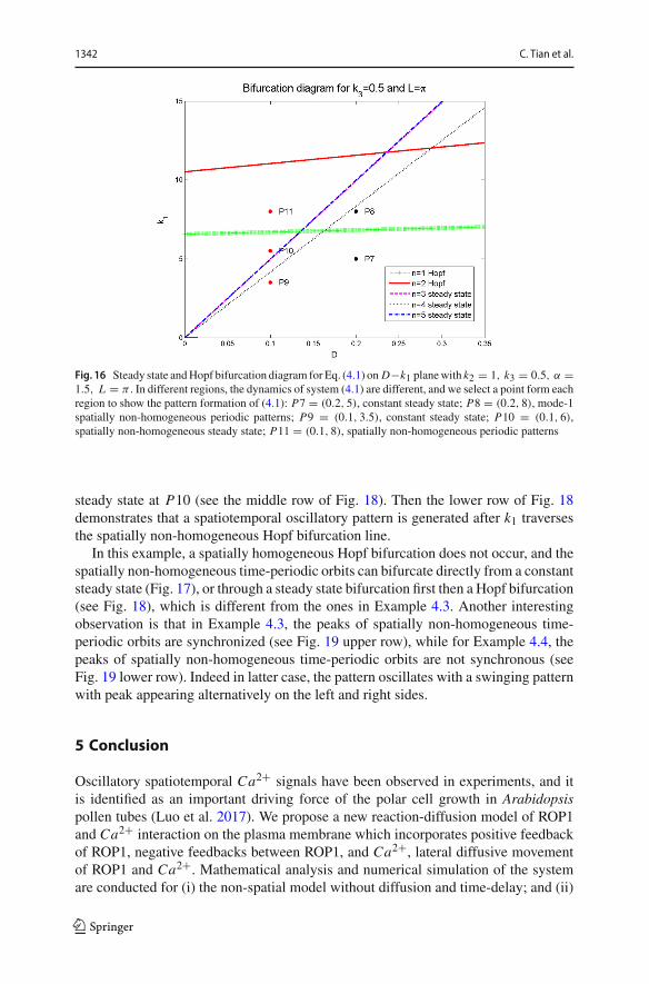
Fig. 16 Steady state andHopf bifurcation diagram for Eq. (4.1) on D−k1 planewith k2 = 1, k3 = 0.5, α =1.5, L = π . In different regions, the dynamics of system (4.1) are different, and we select a point form eachregion to show the pattern formation of (4.1): P7 = (0.2, 5), constant steady state; P8 = (0.2, 8), mode-1spatially non-homogeneous periodic patterns; P9 = (0.1, 3.5), constant steady state; P10 = (0.1, 6),spatially non-homogeneous steady state; P11 = (0.1, 8), spatially non-homogeneous periodic patterns

steady state at P10 (see the middle row of Fig. 18). Then the lower row of Fig. 18demonstrates that a spatiotemporal oscillatory pattern is generated after k1 traversesthe spatially non-homogeneous Hopf bifurcation line.

In this example, a spatially homogeneous Hopf bifurcation does not occur, and thespatially non-homogeneous time-periodic orbits can bifurcate directly from a constantsteady state (Fig. 17), or through a steady state bifurcation first then a Hopf bifurcation(see Fig. 18), which is different from the ones in Example 4.3. Another interestingobservation is that in Example 4.3, the peaks of spatially non-homogeneous time-periodic orbits are synchronized (see Fig. 19 upper row), while for Example 4.4, thepeaks of spatially non-homogeneous time-periodic orbits are not synchronous (seeFig. 19 lower row). Indeed in latter case, the pattern oscillates with a swinging patternwith peak appearing alternatively on the left and right sides.

5 Conclusion

Oscillatory spatiotemporal Ca2+ signals have been observed in experiments, and itis identified as an important driving force of the polar cell growth in Arabidopsispollen tubes (Luo et al. 2017). We propose a new reaction-diffusion model of ROP1and Ca2+ interaction on the plasma membrane which incorporates positive feedbackof ROP1, negative feedbacks between ROP1, and Ca2+, lateral diffusive movementof ROP1 and Ca2+. Mathematical analysis and numerical simulation of the systemare conducted for (i) the non-spatial model without diffusion and time-delay; and (ii)

123


Fig. 17 The dynamics of Eq. (4.1) when D = 0.2, k2 = 1, k3 = 0.5, L = π . (Upper row: P7(0.2, 5)):stable constant steady state; (Lower row: P8(0.2, 8)): spatiotemporal pattern generated by spatially non-homogeneous Hopf bifurcation with n = 1

the spatial model with diffusion, nonlocal effect but without time-delay. The effect oftime-delay is not considered in this paper but will be analyzed in a future work.

It is revealed from mathematical analysis that the non-spatial model could havemultiple steady states because of the degeneracy of the trivial steady state, and alsothe Hill type rate function that Calcium inhibits ROP1. Oscillations also occur inthe non-spatial model as a result of Hopf bifurcation (steady state losing stabil-ity to temporal oscillation). The study of non-spatial models provides a guidancefor parameter selection when detecting spatiotemporal patterns in spatial models.For the spatial reaction-diffusion model, parameter ranges supporting spatially non-homogenous time-periodic solutions are identified via linear stability analysis, andnumerical simulations confirm the existence of stable spatially non-homogenous time-periodic patterns. Some of these patterns show a symmetric spatial profile with peakvalues occurring at two locations, and the peak values oscillates with the time. Thesespatiotemporal characters qualitatively match with experimental data from Yang’s lab(Hwang et al. 2005). Quantitative comparison of numerical simulated solutions andexperimental data, model validation using experimental data as well as fine tuning ofthe reaction-diffusion model will be the next stage of the investigation.

123

1344 C. Tian et al.

Fig. 18 The dynamics of Eq. (4.1) when D = 0.1, k2 = 1, k3 = 0.5, L = π . (Upper row: P9(0.1, 3.5)):stable constant steady state; (Middle row: P10(0.1, 6)): spatially non-homogeneous steady state with twopeaks; (Lower row: P11(0.1, 8)): spatiotemporal pattern with two peaks

123


Fig. 19 The snapshots of the spatiotemporal patterns of Ca2+ at certain moments. (Upper row): a thesnapshots of patterns in Fig. 15a; b the snapshots of patterns in Fig. 15c. (Lower row): c the snapshots ofpatterns in Fig. 17c; d the snapshots of patterns in Fig. 18e

The spatiotemporal pattern formation discovered here also extends the classicalTuring diffusion-induced pattern formation theory. In the standard reaction-diffusionsystem, a spatially non-homogenous time-periodic solution bifurcating from a trivialsteady state is usually not stable, as the only stable time-periodic solution would be thespatially homogenous one. Here we find that the presence of a nonlocal integral term(in the model it represents the total amount of cytoplasmic molecules) could changethis. In our model, a spatially non-homogenous time-periodic solution could be thefirst bifurcating pattern from a stable homogeneous steady state, hence it could be astable pattern. Theoretical study in that aspect will be continued in another work (Shiet al. 2019a) for more general situations.

In this paper a spatiotemporal mathematical model in a one-dimensional spatialdomain is considered, while a more realistic model for the interaction between ROP1and Ca2+ is on a two-dimensional or three-dimensional spatial domain. The simpli-fied one-dimensional model here illustrates the reaction-diffusion pattern formationmechanism, and we expect similar spatiotemporal patterns also occur in the morerealistic two-dimensional or three-dimensional models. This will be verified in ourfuture work.

123

1346 C. Tian et al.

6 Appendix

Proof of Proposition 3.1 In this proposition, we study the number of roots of equation(3.4) with 1 < α < 2. The function f (R) has the properties that

limR→0+ f (R) = −∞ and lim

R→∞ f (R) = ∞. (6.1)

Also, we have the first derivative of f (R) as

f ′(R) = αRα−1 − (α − 1)Rα−2 + k23(α − 2)Rα−3 − k23(α − 3)Rα−4. (6.2)

Leth(R) = αR3 − (α − 1)R2 + k23(α − 2)R − k23(α − 3). (6.3)

So we have f ′(R) = Rα−4h(R).Step 1. There exists a unique x2 > 0 such that h′(R) < 0 for 0 < R < x2, h′(R) > 0for R > x2, and h(R) reaches the global minimum in (0,∞) at R = x2.

Note that the function h(R) has the properties that

h(0) = −k23(α − 3) > 0 and limR→∞ h(R) = ∞, (6.4)

and we have the first derivative of h(R) as

h′(R) = 3αR2 − 2(α − 1)R + k23(α − 2). (6.5)

Sinceα ∈ (1, 2), for (6.5), we have the discriminant�1 = 4(α−1)2−12k23α(α−2) >

0. In this case, h′(R) = 0 must have two roots in (−∞,∞). Notice that2(α − 1)

3α> 0

andk23(α − 2)

3α< 0 so h′(R)must have one negative root and one positive root. Let x2

be the positive root of h′(R) = 0. Since h′(0) = k23(α − 2) < 0, we have h′(R) < 0for 0 < R < x2, h′(R) > 0 for R > x2. Therefore, h(R) decreases for 0 < R < x2,and increases for R > x2. That is to say, if h(x2) ≥ 0, then h(R) ≥ 0 for any R > 0,while h(R) = 0 has two positive solutions if h(x2) < 0.Step 2. There exist k31, k32 > 0 such that

h(x2)

{≥ 0, if k31 < k3 < k32.< 0, if 0 < k3 < k31 or k3 > k32.

(6.6)

Since h′(R) is an quadratic function and the relationship between h(R) and h′(R),we can have following two facts:

x2 =(α − 1) +

√

(α − 1)2 − 3k23α(α − 2)

3α, (6.7)

123


h(x2) =(x23

− α − 1

9α

)

h′(x2) + 6k23α(α − 2) − 2(α − 1)2

9αx2

+ k23(α − 1)(α − 2) − 9k23α(α − 3)

9α. (6.8)

Therefore, we have

h(x2) ≥ 0 (6.9)

⇔ x2 ≤ (α − 1)(α − 2) − 9α(α − 3)

2(α − 1)2 − 6k23α(α − 2)k23 (6.10)

⇔(α − 1) +

√

(α − 1)2 − 3k23α(α − 2)

3α≤ (α − 1)(α − 2) − 9α(α − 3)

2(α − 1)2 − 6k23α(α − 2)k23

(6.11)

⇔ Ak43 + Bk23 + C ≥ 0, (6.12)

where

A =α(α − 2)3 < 0, (6.13)

B =2(α − 1)2(α − 2)2 − 18(α − 1)(α − 2) + 27 > 0, (6.14)

C =(α − 1)3(α − 3) < 0. (6.15)

Notice that the discriminant of the quadratic function Ay2 + By + C is

�2 = [2(α − 1)2(α − 2)2 − 18(α − 1)(α − 2)+27]2 − 4α(α − 1)3(α − 2)3(α − 3)(6.16)

= [2(α − 1)2(α − 2)2 − 18(α − 1)(α − 2) + 27]2− 4(α − 1)4(α − 2)4 + 8(α − 1)3(α − 2)3 (6.17)

> −18(α − 1)(α − 2)[4(α − 1)2(α − 2)2

− 18(α − 1)(α − 2) + 27] + 8(α − 1)3(α − 2)3 (6.18)

= −2(α − 1)(α − 2)[32(α − 1)2(α − 2)2 − 162(α − 1)(α − 2) + 243].(6.19)

Since the discriminant of the quadratic function 32y2 − 162y + 243 is �3 = 1622 −4×32×243 = −4860 < 0, then 32(α −1)2(α −2)2 −162(α −1)(α −2)+243 > 0for any α. Therefore

�2 > −2(α−1)(α−2)[32(α−1)2(α−2)2−162(α−1)(α−2)+243] > 0. (6.20)

So the quadratic equation Ay2+ By+C = 0 has two real-valued solutions k∗31 < k∗

32.

Because k∗31+k∗

32 = − B

A> 0 and k∗

31k∗32 = C

A> 0, then k∗

31 and k∗32 are both positive.

123

1348 C. Tian et al.

Moreover we can have that Ak43 + Bk23 + C ≥ 0 if and only if k∗31 ≤ k23 ≤ k∗

32. Nowlet k31 = √

k∗31 and k32 = √

k∗32, we reach the conclusion in (6.6).

Step 3. We consider the number of roots of equation f (R) = 0 in (3.4) for eachcase in (6.6). In the case where h(x2) ≥ 0, we would have h(R) ≥ 0 for any R > 0because h(R) decreases for 0 < R < x2, and increases for R > x2. That is to say,f ′(R) = Rα−4h(R) > 0 for any R > 0. So f (R) increases for all R > 0. Accordingto property (6.1), f (R) = 0 has one unique positive root.

On the other hand, when h(x2) < 0, h(R) = 0 has two positive solutions. Let 0 <

r1 < x2 < r2 be the solutions of h(R) = 0. Then h(R) > 0 if R ∈ [0, r1)∪ (r2,+∞)

and h(R) < 0 if R ∈ (r1, r2). That is to say,

f ′(R) = Rα−4h(R)

⎧⎨

⎩

> 0, if R ∈ (0, r1),< 0, if R ∈ (r1, r2),> 0, if R ∈ (r2,+∞).

(6.21)

Therefore, f (R) increases for 0 < R < r1, decreases for r1 < R < r2, and increaseswhen R > r2. Then we know that

1. If f (r1) f (r2) > 0, then f (R) = 0 has one unique positive solution.2. If f (r1) f (r2) = 0, then f (R) = 0 has two positive solutions.3. If f (r1) f (r2) < 0, then f (R) = 0 has three positive solutions.

Definel(R) = Rα−3(1 − R)(R2 + k23). (6.22)

Then f (r1) f (r2) = [k2−l(r1)][k2−l(r2)]. Since r1 and r2 are solutions of h(R) = 0,r1 and r2 only depends on α and k3. So there exists k21, k22 which only depends on α,k3 and are defined as

k21 = rα−31 (1 − r1)(r

21 + k23), k22 = rα−3

2 (1 − r2)(r22 + k23), (6.23)

such that

1. If k2 < k21 or k2 > k22, then f (R) = 0 has one unique positive solution.2. If k2 = k21 or k2 = k22, then f (R) = 0 has two positive solutions.3. If k21 < k2 < k22, then f (R) = 0 has three positive solutions.

We claim that 0 < k21 < k22 for 0 < k3 < k31, while k21 < k22 < 0 for k3 > k32.This is equivalent to r1 < r2 < 1 for 0 < k3 < k31, while 1 < r1 < r2 for k3 < k32.Notice that h(1) = 1+k23 > 0, and that h(R) decreases for 0 < R < x2 and increasesfor R > x2. So we only need to prove that h′(1) = α + 2 + k23(α − 2) < 0 for0 < k3 < k31, while h′(1) > 0 for k3 > k32. In fact, k231 and k232 are two positiveroots of equation Ay2 + By +C = 0, where A, B,C are defined as (6.13), (6.14) and(6.15) respectively. Notice that A < 0 and

A

(2 + α

2 − α

)2

+ B

(2 + α

2 − α

)

+C = 32

(

α − 1

4

)2

+ 54α

2 − α> 0, for 1 < α < 2.

(6.24)

123


So k231 <2 + α

2 − α< k232. Therefore, we have

h′(1) = α + 2 + k23(α − 2) > α + 2 + k231(α − 2) > 0, if 0 < k3 < k31, (6.25)

h′(1) = α + 2 + k23(α − 2) < α + 2 + k232(α − 2) < 0, if k3 > k32. (6.26)

So we have proved that 0 < k21 < k22 for 0 < k3 < k31, while k21 < k22 < 0 fork3 > k32. Therefore we reach the conclusion about number of solution of f (R) = 0.

��

Proof of Proposition 3.2 By the Center Manifold Theorem (Page 116 in Perko (2001)),we can compute the center manifold near the equilibrium (0, 0):

C = ϑ(R) = 1

k1(2 − α)R2−α + o(R2−α). (6.27)

Then, by substituting (6.27) into the first equation of the kinetic system (3.1), we obtainthe following scalar system which gives the flow of Eq. (3.1) on the center manifold:

Rt = k1Rα(1 − R) − k1k2

Rϑ2(R)

ϑ2(R) + k23> 0, for 0 < R < δ. (6.28)

Thus, we know that the flow on the center manifold is moving away from the originand it is an unstable orbit.

Next we show that there is an invariant region near R = 0, C > 0 for Eq. (3.1).Define

O =⎧⎨

⎩(R,C) : 0 ≤ R ≤

(k2

2(k23 + δ2)

) 1α−1

C2

α−1 , 0 ≤ C ≤ δ

⎫⎬

⎭.

It is obvious that R = 0 is invariant for (3.1). Then, if C = δ, 0 ≤ R ≤(

k22(k23 + δ2)

) 1α−1

δ2

α−1 , since 1 < α < 2 then 2α−1 > 1, so one can choose δ > 0

small enough so that

(k2

2(k23 + δ2)

) 1α−1

δ2

α−1 ≤ δ. By using C = δ, we have C ′ < 0.

123

1350 C. Tian et al.

On the boundary R =(

k22(k23 + δ2)

) 1α−1

C2

α−1 , we have

d

dt

(R

α−12

C

)

=α−12 CR

α−32 R′ − R

α−12 C ′

C2 = Rα−32

C2

(α − 1

2CR′ − RC ′

)

= Rα−32

C2

[α − 1

2Ck1

(

Rα − Rα+1 − k2RC2

C2 + k23

)

− R2 + CR

]

≤ Rα−32

C

[α − 1

2k1

(

Rα − k2RC2

C2 + k23

)

+ R

]

≤ Rα−32

C

[

(α − 1)k1Rα − (α − 1)k1k2RC2

2(C2 + k23)

]

≤ Rα−32

C

[

(α − 1)k1

(

Rα − (α − 1)k1k2RC2

2(δ2 + k23)

)]

= (α − 1)Rα−12 k1C

2

[Rα−1

C2 − k22(δ2 + k23)

]

= 0,

and thefirst inequality holds for R small enough: R < α−12 k1Rα . The above calculation

implies that the dynamics of (3.1) is inward on R =(

k22(k23 + δ2)

) 1α−1

C2

α−1 . This

shows that O is an invariant region for Eq. (3.1), and any orbit in O converges tothe origin. It is also clear that when R = 0, C > 0 (the positive C-axis), we have(Rt ,Ct ) = (0,−C). So we know that all the solutions starting from R = 0, C > 0will always stay on this curve and eventually converge to the origin. One can choosea maximum orbit R = hs(C) so that all orbits such that 0 ≤ R ≤ hs(C) converge tothe origin. Then other trajectories exhibits saddle behavior near the origin. ��Proof of Theorem 3.3 First, we look at the determinant of the Jacobian matrixJ (R j , R j ): Det(J (R j , R j )) = k1R j ( f ′

2(R j ) − f ′1(R j )), where f1, f2 are defined

in (3.6). From (3.6), we have

f2(R) − f1(R) = k2R2

R2 + k23− Rα−1(1 − R) (6.29)

⇔ f (R) = k2 − Rα−3(1 − R)(R2 + k23) = R2 + k23R2 ( f2(R) − f1(R)) (6.30)

⇔ f ′(R) = −2k23R3 ( f2(R) − f1(R)) + R2 + k23

R2 ( f ′2(R) − f ′

1(R)). (6.31)

From (6.30), we know that f2(R) − f1(R) = 0 when f (R) = 0. Since positivesteady states (R j , R j ) ( j = 1, 2, 3) satisfy f (R j ) = 0, we have f2(R j )− f1(R j ) = 0.

123


Therefore, from (6.31), we know

f ′(R j ) > 0 ⇔ f ′2(R j ) − f ′

1(R j ) > 0 ⇔ Det(J (R j , R j )) > 0;f ′(R j ) = 0 ⇔ f ′

2(R j ) − f ′1(R j ) = 0 ⇔ Det(J (R j , R j )) = 0;

f ′(R j ) < 0 ⇔ f ′2(R j ) − f ′

1(R j ) < 0 ⇔ Det(J (R j , R j )) < 0.

According to the proof of Proposition 3.1, we have the following result ofDet(J (R j , R j )): there exists a constant k31 > 0 such that

1. If 0 < k3 < k31, then there exists r1 and r2, which are two positive solutions ofh(R) = 0, such that

(a) f ′(R) > 0 ⇒ Det(J (R, R)) > 0 for R ∈ (0, r1) ∪ (r2, 1);(b) f ′(R) < 0 ⇒ Det(J (R, R)) < 0 for R ∈ (r1, r2).

2. If k31 < k3, then for any 0 < R < 1, we always have f ′(R) > 0 ⇒Det(J (R, R)) > 0.

Here we want to point out that from (6.23), we have k2(r1) = k21 and k2(r2) = k22.Next we look at the trace of Jacobianmatrix (3.5): Tr(J (R j ,C j )) = k1R j f ′

1(R j )−1. Define a new function

g(R) = R f ′1(R) = Rα−1[(α − 1) − αR]. (6.32)

We observe that g(R) has the following properties:

g(0) = 0, g

(α − 1

α

)

= 0, and limR→∞ g(R) = ∞. (6.33)

Also we have the first derivative of g(R) as

g′(R) = Rα−2[(α − 1)2 − α2R]. (6.34)

Hence the function g(R) increases for 0 < R <

(α − 1

α

)2

and decreases for R >

(α − 1

α

)2

. So g(R) achieves itsmaximumat R =(

α − 1

α

)2

with g

((α − 1

α

)2)

=(

α − 1

α

)2α−1

.

Therefore we conclude that

1. If k1 <

(α

α − 1

)2α−1

, then

Tr(J (R, R)) = k1g(R) − 1 <

(α

α − 1

)2α−1 (α − 1

α

)2α−1

− 1 = 0. (6.35)

123

1352 C. Tian et al.

2. If k1 >

(α

α − 1

)2α−1

, then there exists 0 < R̃1 < R̃2, such that g(R̃1) =

g(R̃2) = 1

k1. Therefore,

(a) If R̃1 < R < R̃2, then Tr(J (R, R)) = k1g(R) − 1 > k1g(R̃1) = 0.(b) If 0 < R < R̃1 or R̃2 < R < 1, then Tr(J (R, R)) = k1g(R)−1 < k1g(R̃1) =

0.

��Proof of Proposition 3.4 From the proof of Theorem 3.3, we can easily get Part 1 inProposition 3.4. So here we only discuss Part 2: the case that 0 < k3 < k31. SinceDet(J (R2,C2)) < 0, the steady state (R2,C2) is always a saddle point. Sowe focus onthe positive steady states (R1,C1) and (R3,C3). To prove the results in Proposition 3.4,we need to determine the order of the possible bifurcation points: r1, r2, R̃1 and R̃2,where r1 and r2 are the steady state bifurcation points satisfying h(r1) = h(r2) = 0with h(R) defined in (6.3), and R̃1, R̃2 are possible Hopf bifurcation points satisfyingg(R̃1) = g(R̃2) = 1/k1. Then, by the results of Theorem 3.3, we can obtain thestability of each steady state.

First, we prove that g(r1) > g(r2) always holds. From the definition of h(R), weknow that

h(r1) = αr31 − (α − 1)r21 + k23(α − 2)r1 − k23(aα − 3) = 0. (6.36)

Multiplying (6.36) by rα−31 , we have

αrα1 − (α − 1)rα−1

1 + k23(α − 2)rα−21 − k23(aα − 3)rα−3

1 = 0, (6.37)

which together with g(r1) = −αrα1 + (α − 1)rα−1

1 from (6.32) implies that

g(r1) = k23(α − 2)rα−21 − k23(α − 3)rα−3

1 . (6.38)

Define

G(R) = k23(α − 2)Rα−2 − k23(α − 3)Rα−3, R ∈ (0, 1), α ∈ (1, 2). (6.39)

By direct calculation, we have G ′(R) = k23(α − 2)2Rα−3 − k23(α − 3)2Rα−4 and

G ′(R) < 0 for R ∈(

0,(

α−3α−2

)2)

⊃ (0, 1). Therefore, G(R) is strictly decreasing for

R ∈ (0, 1). By the fact that 0 < r1 < r2 < 1, immediately we reach the conclusionthat g(r1) > g(r2).

Nowwe consider the case that 0 < k3 < k31 which implies the existence ofmultiplesteady states. For the convenience of discussion, we define

g̃(R) = g(R) − 1/k1, (6.40)

123


then we know that g̃ has two zeros R̃1 and R̃2. For the order of r1, r2, R̃1 and R̃2, wehave the following six possible situations:

(i) r1 < r2 < R̃1 < R̃2. We show that this case will not happen. By the property

of h(R), it is not difficult to verify that h((

α−1α

)2)

> 0 = h(r2), so we know

that(

α−1α

)2< r2. Because

(α−1α

)2is the maximum point of g̃(R) and R̃1 is

the smallest root of g̃(R), so we have R̃1 < r2 which is a contradiction to theassumption.

(ii) r1 < R̃1 < r2 < R̃2. By the fact that g̃(R) > 0 for R ∈ (R̃1, R̃1) and g(R) < 0for R ∈ (0, R̃1) ∪ (R̃2, 1), it is easy to obtain that g̃(r1) < 0 since r1 < R̃1,which is equivalent to k1 < 1/g(r1). Also, by g̃(r2) > 0, we have k1 > 1/g(r2).However, it has been proved that g(r1) > g(r2), so the set (1/g(r2), 1/g(r1)) isempty, which means that this case cannot happen.

(iii) R̃1 < r1 < r2 < R̃2 (see Fig. 7c). Because that r1, r2 ∈ (R̃1, R̃2), so we haveg̃(r1) > 0 and g̃(r2) > 0, which is equivalent to k1 > 1/g(r2). In this case,by Theorem 3.3, we know that Hopf bifurcations occur at both of (R1, R1) and(R3, R3).

(iv) R̃1 < r1 < R̃2 < r2 (see Fig. 7d). By similar argument, since r1 ∈ (R̃1, R̃2)

and r2 > R̃2, we can obtain that g̃(r1) > 0 and g̃(r2) < 0 which imply thatk1 ∈ (1/g(r1), 1/g(r2)). In this case, from R̃1 < r1 < R̃2 < r2 and Theorem 3.3,a Hopf bifurcation only occurs at (R3, R3) and does not occur at (R1, R1).

(v) r1 < R̃1 < R̃2 < r2 (see Fig. 7e). Similarly, we have g̃(r1) < 0 and g̃(r2) < 0,then it can be inferred that k11 < k1 < 1/g(r1). In this case, no Hopf bifurcation

can occur. Also, we have(

α−1α

)2> r1 in this case, which will be used later.

(vi) R̃1 < R̃2 < r1 < r2 (see Fig. 7f). In this case, we still have k11 < k1 < 1/g(r1),

but the difference with case (v) is that(

α−1α

)2< r1. In this case, two Hopf

bifurcations occur at (R1, R1).

So in order to distinguish the last two cases, we define k̃3 to be the value of k3 such

that r1 = (α−1α

)2, and it is easy to calculate that k̃3 is given by (3.16). So case (v) is

for 0 < k3 < k̃3 which is equivalent to r1 <(

α−1α

)2and case (vi) is for k̃3 < k3 < k31

which implies r1 >(

α−1α

)2. Also we must have that k̃3 < k31. Suppose not, then

first we assume that k3 > k32, then h(R) = 0 has two positive solutions, but both ofthem should be bigger than 1 and here we have 0 < R < 1 which is a contradiction.If k31 < k3 < k32, then h(R) = 0 has no roots, so it contradicts with the fact that

h(R) = 0 has one of positive roots at (α − 1

α)2 < 1 when k3 = k̃3. Therefore, we can

conclude that k̃3 < k31. Finally if 0 < k1 < k11, then g̃(R) has no zeros, (R1, R1) and(R3, R3) are both always linearly stable and Hopf bifurcation will not occur, which issimilar to (v) above.

In summary the case (c) is implied by (iii) above, case (d) is implied by (iv) above,case (e) is implied by (v) and the case of 0 < k1 < k11, and case (f) is implied by (vi)above. The proof is completed. ��

123

1354 C. Tian et al.

References

Altschuler SJ, Angenent SB,Wang Y,Wu LF (2008) On the spontaneous emergence of cell polarity. Nature454(7206):886–889

Busenberg S, HuangW-Z (1996) Stability and Hopf bifurcation for a population delay model with diffusioneffects. J Differ Equ 124(1):80–107

Chen S-S, Lou Y, Wei J-J (2018) Hopf bifurcation in a delayed reaction-diffusion-advection populationmodel. J Differ Equ 264(8):5333–5359

Chen S-S, Shi J-P (2012) Stability and Hopf bifurcation in a diffusive logistic population model withnonlocal delay effect. J Differ Equ 253(12):3440–3470

Chen S-S, Shi J-P,Wei J-J (2013) Time delay-induced instabilities andHopf bifurcations in general reaction-diffusion systems. J Nonlinear Sci 23(1):1–38

Chen S-S, Shi J-P, Wei J-J (2014) Bifurcation analysis of the Gierer-Meinhardt system with a saturation inthe activator production. Appl Anal 93(6):1115–1134

Chen S-S, Yu J-S (2016a) Stability analysis of a reaction-diffusion equation with spatiotemporal delay andDirichlet boundary condition. J Dyn Differ Equ 28(3–4):857–866

Chen S-S, Yu J-S (2016b) Stability and bifurcations in a nonlocal delayed reaction-diffusion populationmodel. J Differ Equ 260(1):218–240

Chou C-S, Nie Q, Yi T-M (2008)Modeling robustness tradeoffs in yeast cell polarization induced by spatialgradients. PloS One 3(9):e3103

Ding D-Q, Shi J-P, Wang Y (2017) Bistability in a model of grassland and forest transition. J Math AnalAppl 451(2):1165–1178

Edelstein-Keshet L, Holmes WR, Zajac M, Dutot M (2013) From simple to detailed models for cell polar-ization. Philos Trans R Soc Lond B Biol Sci 368(1629):20130003

Feijó JA, Sainhas J, Holdaway-Clarke T, Cordeiro MS, Kunkel JG, Hepler PK (2001) Cellular oscillationsand the regulation of growth: the pollen tube paradigm. Bioessays 23(1):86–94

Gierer A, Meinhardt H (1972) A theory of biological pattern formation. Biol Cybern 12(1):30–39Goryachev AB, Pokhilko AV (2008) Dynamics of Cdc42 network embodies a Turing-type mechanism of

yeast cell polarity. FEBS Lett 582(10):1437–1443Gu Y, Fu Y, Dowd P, Li S-D, Vernoud V, Gilroy S, Yang Z-B (2005) A rho family gtpase controls actin

dynamics and tip growth via two counteracting downstream pathways in pollen tubes. J Cell Biol169(1):127–138

Guo S-J (2015) Stability and bifurcation in a reaction-diffusion model with nonlocal delay effect. J DifferEqu 259(4):1409–1448

Holmes WR, Edelstein-Keshet L (2016) Analysis of a minimal Rho-GTPase circuit regulating cell shape.Phys Biol 13(4):046001

Hwang J-U, Gu Y, Lee Y-J, Yang Z-B (2005) Oscillatory ROP GTPase activation leads the oscillatorypolarized growth of pollen tubes. Mol Biol Cell 16(11):5385–5399

Jilkine A, Marée AFM, Edelstein-Keshet L (2007) Mathematical model for spatial segregation of the Rho-family GTPases based on inhibitory crosstalk. Bull Math Biol 69(6):1943–1978

Jin J-Y, Shi J-P, Wei J-J, Yi F-Q (2013) Bifurcations of patterned solutions in the diffusive Lengyel-Epsteinsystem of CIMA chemical reactions. Rocky Mt J Math 43(5):1637–1674

Kondo S, Miura T (2010) Reaction-diffusion model as a framework for understanding biological patternformation. Science 329(5999):1616–1620

Li H, Lin Y-K, Heath RM, Zhu M X, Yang Z-B (1999) Control of pollen tube tip growth by a rop gtpase–dependent pathway that leads to tip-localized calcium influx. Plant Cell 11(9):1731–1742

Li X, Wang H, Zhang Z, Hastings A (2014) Mathematical analysis of coral reef models. J Math Anal Appl416(1):352–373

Lo W-C, Park H-O, Chou C-S (2014) Mathematical analysis of spontaneous emergence of cell polarity.Bull Math Biol 76(8):1835–1865

Ludwig D, Jones DD, Holling CS (1978) Qualitative analysis of insect outbreak systems: the spruce bud-worm and forest. J Anim Ecol 47(1):315–332

Luo N, Yan A et al (2017) Exocytosis-coordinated mechanisms for tip growth underlie pollen tube growthguidance. Nat Commun 8(1):1687

Maini P, Painter K, Chau H (1997) Spatial pattern formation in chemical and biological systems. J ChemSoc Faraday Trans 93(20):3601–3610

123


Mogilner A, Allard J, Wollman R (2012) Cell polarity: quantitative modeling as a tool in cell biology.Science 336(6078):175–179

Moore TI, Chou C-S, Nie Q, Jeon NL, Yi T-M (2008) Robust spatial sensing of mating pheromone gradientsby yeast cells. PloS One 3(12):e3865

Mori Y, Jilkine A, Edelstein-Keshet L (2011) Asymptotic and bifurcation analysis of wave-pinning in areaction-diffusion model for cell polarization. SIAM J Appl Math 71(4):1401–1427

Mumby PJ, Hastings A, Edwards HJ (2007) Thresholds and the resilience of Caribbean coral reefs. Nature450(7166):98–101

Perko L (2001) Differential equations and dynamical systems, texts in applied mathematics, vol 7, 3rd edn.Springer, New York

Rätz A, Röger M (2012) Turing instabilities in a mathematical model for signaling networks. J Math Biol65(6–7):1215–1244

Scheffer M, Carpenter S, Foley JA, Folke C, Walker B (2001) Catastrophic shifts in ecosystems. Nature413(6856):591–596

Scheffer M, Hosper SH, Meijer ML, Moss B, Jeppesen E (1993) Alternative equilibria in shallow lakes.Trends Ecol Evol 8(8):275–279

Seirin Lee S, Gaffney EA, Baker RE (2011) The dynamics of Turing patterns for morphogen-regulatedgrowing domains with cellular response delays. Bull Math Biol 73(11):2527–2551

Shi Q-Y, Shi J-P, Song Y-L (2017) Hopf bifurcation in a reaction-diffusion equation with distributed delayand Dirichlet boundary condition. J Differen Equ 263(10):6537–6575

Shi Q-Y, Shi J-P, Song Y-L (2019a) , Effect of spatial average on the spatiotemporal pattern formation ofreaction-diffusion systems, Preprint

Shi Q-Y, Shi J-P, Song Y-L (2019b) Hopf bifurcation and pattern formation in a diffusive delayed logisticmodel with spatial heterogeneity. Discrete Contin Dyn Syst Ser B 24(2):467–486

Simonett G (1995) Center manifolds for quasilinear reaction-diffusion systems. Differ Integral Equ8(4):753–796

Staver AC, Archibald S, Levin SA (2011a) The global extent and determinants of savanna and forest asalternative biome states. Science 334(6053):230–232

Staver AC, Archibald S, Levin SA (2011b) Tree cover in sub-Saharan Africa: rainfall and fire constrainforest and savanna as alternative stable states. Ecology 92(5):1063–1072

Su Y, Wei J-J, Shi J-P (2009) Hopf bifurcations in a reaction-diffusion population model with delay effect.J Differ Equ 247(4):1156–1184

Turing AM (1952) The chemical basis of morphogenesis. Philos Trans R Soc Lond Ser B 237(641):37–72Wang J-F, Shi J-P, Wei J-J (2011) Dynamics and pattern formation in a diffusive predator-prey system with

strong Allee effect in prey. J Differ Equ 251(4–5):1276–1304Wang J-F, Wei J-J, Shi J-P (2016) Global bifurcation analysis and pattern formation in homogeneous

diffusive predator-prey systems. J Differ Equ 260(4):3495–3523Xiao Z, Brunel N, Yang Z-B. Cui X.-P (2016) Constrained nonlinear and mixed effects of differential

equation models for dynamic cell polarity signaling, arXiv:1605.00185Yan A, Xu G-S, Yang Z-B (2009) Calcium participates in feedback regulation of the oscillating ROP1 Rho

GTPase in pollen tubes. Proc Natl Acad Sci U.S.A. 106(51):22002–22007YanX-P, LiW-T (2010) Stability of bifurcating periodic solutions in a delayed reaction-diffusion population

model. Nonlinearity 23(6):1413–1431Yang Z-B (2008) Cell polarity signaling in arabidopsis. Annu Rev Cell Deve Biol 24:551–575Yi F-Q, Gaffney E, Seirin-Lee S (2017) The bifurcation analysis of Turing pattern formation induced by

delay and diffusion in the Schnakenberg system. Discrete Contin Dyn Syst Ser B 22(2):647–668Yi F-Q,Wei J-J, Shi J-P (2009)Bifurcation and spatiotemporal patterns in a homogeneous diffusive predator-

prey system. J Differ Equ 246(5):1944–1977Yi T-M, Chen S-Q, Chou C-S, Nie Q (2007) Modeling yeast cell polarization induced by pheromone

gradients. J Stat Phys 128(1–2):193–207ZhengZ-Z,ChouC-S,YiT-M,NieQ (2011)Mathematical analysis of steady-state solutions in compartment

and continuum models of cell polarization. Math Biosci Eng 8(4):1135–1168Zhou J, Shi J-P (2015) Pattern formation in a general glycolysis reaction-diffusion system. IMA J Appl

Math 80(6):1703–1738

Publisher’s Note Springer Nature remains neutral with regard to jurisdictional claims in published mapsand institutional affiliations.

123

http://arxiv.org/abs/1605.00185

spatiotemporal dynamics of a reaction-diffusion model of ... · a reaction-diffusion model is...

Documents