arX

iv:1

702.

0566

2v3

[st

at.A

P] 6

Nov

201

7

Spatial modeling of shot conversion in soccer to single

out goalscoring ability

Soudeep Deb ∗

Department of Statistics,The University of Chicago,

5747 S Ellis Ave,

Chicago, IL, USA. 60615Phone: +1(312)709-0673

Debangan Dey †

Department of Biostatistics,Johns Hopkins Bloomberg School of Public Health,

615 N Wolfe Street,Baltimore, MD, USA. 2120

Phone: +1 (917)292-7447

Abstract

Goals are results of pin-point shots and it is a pivotal decision in soccer when, how andwhere to shoot. The main contribution of this study is two-fold. At first, after showingthat there exists high spatial correlation in the data of shots across games, we introducea spatial process in the error structure to model the probability of conversion from ashot depending on positional and situational covariates. The model is developed usinga full Bayesian framework. Secondly, based on the proposed model, we define two newmeasures that can appropriately quantify the impact of an individual in soccer, byevaluating the positioning senses and shooting abilities of the players. As a practicalapplication, the method is implemented on Major League Soccer data from 2016/17season.

Keywords: Soccer analytics, Probit regression, Bayesian modeling, MCMC, Spatialcorrelation.

∗Email: sdeb@uchicago.edu; Corresponding author†Email: ddey1@jhu.edu

1

1 Introduction

Association football or Soccer is arguably the most popular sport in the world. Along withthe excitement involved with the international fixtures, millions of viewers across the worldalso watch the club football on a regular basis. And with the ever-growing competitivenature of the sport, the field of soccer analytics is becoming more important with everypassing day. The most interesting aspect about soccer is that it is a dynamic game and ateam’s success relies both on team strategies and individual player contributions. Hence, itis generally more difficult to develop sophisticated statistical methods for soccer as comparedto, say baseball, where events are more discrete.

In soccer, the soccer-ball is certainly like the principal atom in the game, around which theplayers on the pitch trace their path. In soccer, a shot gives momentum to the atom ofthe game, read soccer ball, to reach its intended destination, the back of the net. In thisaspect, shooting ability of a player has always been a key factor in building team strategies,as the outcome of a game is decided based on the number of goals scored by the two teams.So, it is immensely important to identify players who have great positioning sense and cansuccessfully convert the chances to score more frequently than others. And there comes theneed to define a measure which can capture the information about a player’s positioningsense and how good he is in converting shots to goals.

A simple way of looking at this problem is to calculate the proportion of shots one convertssuccessfully, which works around the assumption that probability of scoring a goal is thesame for all shots taken by a certain player. While it gives some idea about the efficiencyof a striker, it has its shortcomings and would fail to serve the purpose from many aspects.For example, this crude measure only gives the percentage of shots converted successfully,but it does not tell anything about the players’ positioning senses. Besides, this measurefails to identify difficulty of chances. For example, a player scoring 2 goal from 4 shots, allfrom several yards out of the box is considered equally efficient as another who scores 1 from2 shots from inside the box, and that is definitely not the case. Naturally, one should takeinto account many other factors - location, time, type of play, how the shot was taken andopponents being some examples - to investigate the conversion rates of soccer players.

While the problem of predicting goals has not been overwhelmingly explored in soccer, thereare some studies that have tried to predict the outcome of an average shot from an averageplayer from a particular position on the pitch in a particular situation. Of course, thereare limitations as we do not know the shot speed, the position of defenders and the exactgoalkeeper position but it is worthy to check how much variance we can explain from theexisting covariates which, at the first look, seem to be really important. Current researchersin this field have taken various routes to assign a goal-scoring probability to a particular shotand finally, worked on to develop an Expected Goals (ExpG) metric for a team or a player.

In general, there are different types of discrete regression models that people have used so far.For example, Goddard (2005) used bivariate Poisson and ordered probit regression models toforecast number of goals scored and conceded in soccer matches based on different covariates.The author here analyzed data from English football and learned that the number of goals

2

in a match depends mostly on the recent home performances of the home side and the recentaway performances of the away side. In another match-level study, Williams and Walters(2011) studied the effects of altitude on the result of soccer matches in South America. Takinga regression-based approach for change in altitude of the away side, they showed that thewin probability decreases significantly for an away team traveling up, while traveling downdoes not have a significant impact on the results.

Player-related or shot-related approaches have been studied by a few authors as well. Oneof the most popular methods in this regard is a study in American Soccer Analysis (2016).Analyzing data from the Major League Soccer (MLS), the authors showed that the shotconversion rates significantly depend on many factors, including the distance, angle and thebody part used when a shot is taken. Simple logistic regression techniques were the maincomponents of this study. In an earlier paper, Moura et al. (2007) dealt with data fromBrazilian first division championship matches and analyzed shots to goal strategies based onthe field position from where the ball was collected and the length of the passing sequenceleading to a goal. Contrary to the popular belief, they found that the ball possessionsresulting in shots to goal usually start in the defensive field of the scoring teams. So far asthe passing sequences are concerned, this study showed that either short (2 to 5) or verylong (10 or more) sequences significantly improve the conversion rates. This second findingcorroborated what Hughes and Franks (2005) found before.

Finally, we cite two works that used the situation in a small time-window just preceding theevent of interest. First, Jordet et al. (2013) used English Premier League data to investigatehow visual exploratory behaviors before receiving the ball affect the probability of completingthe next pass. They found that the players who show extensive visual exploratory behaviorsright before receiving a ball are more successful in completing a pass. In another recentstudy, Lucey et al. (2014) analyzed the spatiotemporal patterns of the ten-second windowof play before a shot was fired. They extracted some strategic features from the data andused them to present a method that estimates the likelihood of a team scoring a goal. Thisstudy showed that not only is the game phase (corner, free-kick, open-play, counter attacketc.) important, but the features such as defender proximity, interaction of surroundingplayers and speed of play coupled with the shot location also play an impact on determiningthe likelihood of a team scoring a goal. A few more relevant discussions can be found inLeitner et al. (2010), Clark et al. (2013), Lasek et al. (2013) and Brooks et al. (2016).

In this study, we want to look at the problem of modeling shot conversion rates from aslightly different point of view. While each of the above models has its advantages, thereare some limitations too. In order to perform the last two methods, one would need theplayer tracking data from some reputable source and that requires a considerable amount ofmoney. On the other hand, usual binary regression based approaches often show a lack offit and fail to have good predictive abilities. This has been discussed more in Section 3.

Our primary goal here is to build a model that fits the data well, identifies the factorssignificantly affecting the shot conversion rate and provides an estimate of the probability ofscoring a goal if the location and other details are given. In this regard, we use a spatiallycorrelated error process in the binary regression model. Another key contribution of thispaper is to quantify the impact of an individual in soccer. In particular, we define two new

3

measures that evaluate the positioning senses and the goal-scoring abilities of the players.As a practical application, we would implement our model, in conjunction with the measureswe devise, to Major League Soccer (MLS) data from 2016/17 season.

The paper is organized as follows. A brief description of the data and some exploratoryanalysis are provided in the next section. In Section 3, we provide motivations behindour idea of including a spatial correlation term in a probit regression model. The proposedmethod and the measures to evaluate shooters’ efficiency are presented in Section 4. Detailedanalysis of the data using the proposed model is carried out in Section 5 while the final sectionincludes a discussion, along with some important concluding remarks.

2 Data

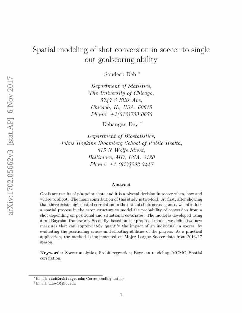
Throughout this study, we use the data for the first half of the MLS 2016/17 season. Sincethe focus is on the shots to goal conversions, relevant information for all shots (excludingpenalties, own goals and cases with some missing data) and their outcomes - encoded asgoal or miss - are recorded. But, we choose to exclude cases when a shot was taken frombeyond the half line, for often these shots are simply the results of some unusual mess-upof the opponent side or the result of a moment of some striker’s presence of mind. In otherwords, a player will not take a shot from beyond the center line unless he is handed a goldenopportunity and naturally, such a shot has a higher probability of being converted. So,including these instances are likely to affect our conclusions. After removing these events,the data comprised of 3957 attempts at goal, among which 482 were converted successfully(approximately 12.18% of the total number of shots). A heat map is shown in Figure 1 toshow the proportions of goal scored from different locations in the field.

0.0

0.2

0.4

0.6

0.8

Proportion of goals based on locations

Figure 1: Heat map of the full data: Total number of attempts were 3957, among which 482were goals and 3475 were misses. Each pixel represents the proportion of goals scored fromthat position, color coded on a scale from 0% (white) to 100% (black).

4

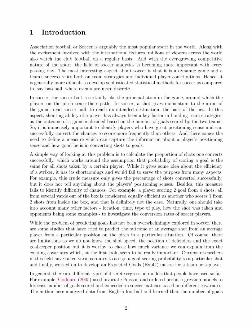
Then, in order to fit an appropriate model, it is crucial to identify possible factors affectingthe conversion of a shot. For that, the first thing we considered are the distance and angleof the location from where a shot is taken. The way we evaluated these two covariates isdisplayed on the left panel of Figure 2. It should be noted that this definition of the angle andthe distance of a shot helps us consider them as uncorrelated covariates in this study. Theright panel of the same figure shows another important covariate in our study, the keeper’sreach. It is evaluated as the shortest distance the goalkeeper has to cover if he stands at thebest position corresponding to the location of the shot.

Distance and angle

X

O

Y

Keepers’s reach

X

O

S

shotbisector

Figure 2: For location X, the distance is evaluated as the Euclidean distance between X andthe center (O) of the goalline, while the angle (with appropriate sign) is calculated as theangle XO makes with OY, the line that bisects the field horizontally.

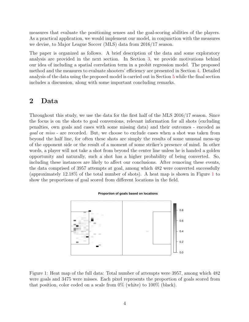
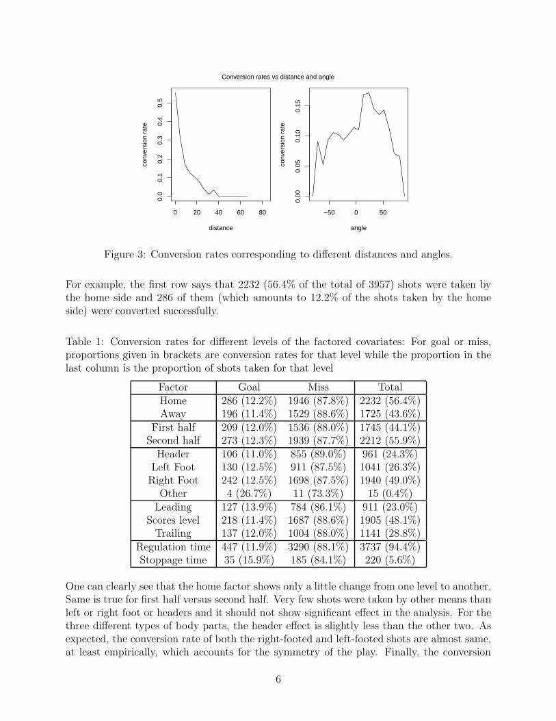
Further, exploratory analysis suggested that a transformation of variable is needed for thedistance and the angle of a shot. Similar to the study by American Soccer Analysis (2016),we found that it is more appropriate to model the conversion rates as linear function of thelogarithm of distance and cosine of angles instead of the usual values. The plots in Figure 3support this.

In addition to the distance, angle and keeper’s reach, there are information on several othercovariates and five of them are considered in this study - if it is a home game, the half ofplay when the shot is taken, body part used in the shot (header, left foot, right foot orother), goal difference at the time of the shot i.e. whether the shooter’s team is leading,level or trailing, if the shot takes place during the stoppage time and the proportion of shotsconverted against the same opponent so far.

Note that the set of covariates we are using includes several situational covariates (home oraway, half of the game, goal difference, and the stoppage time) while the last covariate takesinto account the strength of the opposing teams and helps us to identify if it significantlyaffects the rate of conversion.

A quick summary of the total number and the proportions of shots converted for differentlevels of the aforementioned five factored covariates in the study are presented in Table 1.

5

0 20 40 60 80

0.0

0.1

0.2

0.3

0.4

0.5

distance

conv

ersi

on r

ate

−50 0 50

0.00

0.05

0.10

0.15

angle

conv

ersi

on r

ate

Conversion rates vs distance and angle

Figure 3: Conversion rates corresponding to different distances and angles.

For example, the first row says that 2232 (56.4% of the total of 3957) shots were taken bythe home side and 286 of them (which amounts to 12.2% of the shots taken by the homeside) were converted successfully.

Table 1: Conversion rates for different levels of the factored covariates: For goal or miss,proportions given in brackets are conversion rates for that level while the proportion in thelast column is the proportion of shots taken for that level

Factor Goal Miss TotalHome 286 (12.2%) 1946 (87.8%) 2232 (56.4%)Away 196 (11.4%) 1529 (88.6%) 1725 (43.6%)

First half 209 (12.0%) 1536 (88.0%) 1745 (44.1%)Second half 273 (12.3%) 1939 (87.7%) 2212 (55.9%)Header 106 (11.0%) 855 (89.0%) 961 (24.3%)Left Foot 130 (12.5%) 911 (87.5%) 1041 (26.3%)Right Foot 242 (12.5%) 1698 (87.5%) 1940 (49.0%)

Other 4 (26.7%) 11 (73.3%) 15 (0.4%)Leading 127 (13.9%) 784 (86.1%) 911 (23.0%)

Scores level 218 (11.4%) 1687 (88.6%) 1905 (48.1%)Trailing 137 (12.0%) 1004 (88.0%) 1141 (28.8%)

Regulation time 447 (11.9%) 3290 (88.1%) 3737 (94.4%)Stoppage time 35 (15.9%) 185 (84.1%) 220 (5.6%)

One can clearly see that the home factor shows only a little change from one level to another.Same is true for first half versus second half. Very few shots were taken by other means thanleft or right foot or headers and it should not show significant effect in the analysis. For thethree different types of body parts, the header effect is slightly less than the other two. Asexpected, the conversion rate of both the right-footed and left-footed shots are almost same,at least empirically, which accounts for the symmetry of the play. Finally, the conversion

6

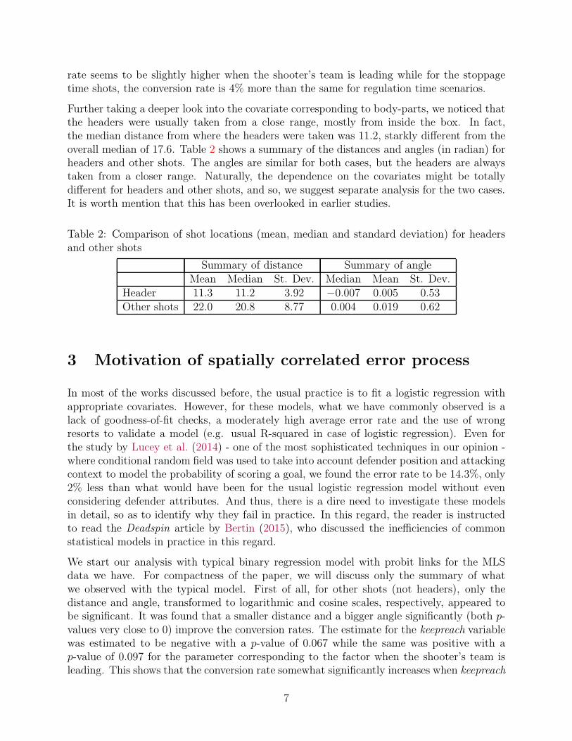
rate seems to be slightly higher when the shooter’s team is leading while for the stoppagetime shots, the conversion rate is 4% more than the same for regulation time scenarios.

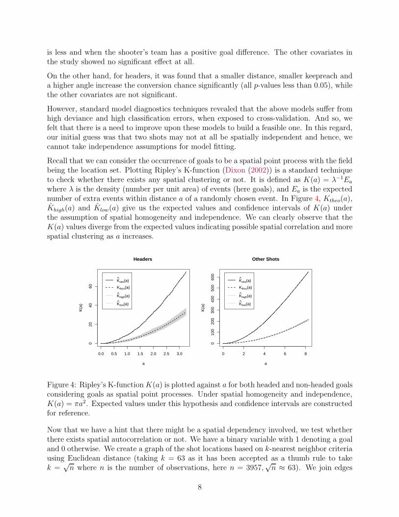
Further taking a deeper look into the covariate corresponding to body-parts, we noticed thatthe headers were usually taken from a close range, mostly from inside the box. In fact,the median distance from where the headers were taken was 11.2, starkly different from theoverall median of 17.6. Table 2 shows a summary of the distances and angles (in radian) forheaders and other shots. The angles are similar for both cases, but the headers are alwaystaken from a closer range. Naturally, the dependence on the covariates might be totallydifferent for headers and other shots, and so, we suggest separate analysis for the two cases.It is worth mention that this has been overlooked in earlier studies.

Table 2: Comparison of shot locations (mean, median and standard deviation) for headersand other shots

Summary of distance Summary of angleMean Median St. Dev. Median Mean St. Dev.

Header 11.3 11.2 3.92 −0.007 0.005 0.53Other shots 22.0 20.8 8.77 0.004 0.019 0.62

3 Motivation of spatially correlated error process

In most of the works discussed before, the usual practice is to fit a logistic regression withappropriate covariates. However, for these models, what we have commonly observed is alack of goodness-of-fit checks, a moderately high average error rate and the use of wrongresorts to validate a model (e.g. usual R-squared in case of logistic regression). Even forthe study by Lucey et al. (2014) - one of the most sophisticated techniques in our opinion -where conditional random field was used to take into account defender position and attackingcontext to model the probability of scoring a goal, we found the error rate to be 14.3%, only2% less than what would have been for the usual logistic regression model without evenconsidering defender attributes. And thus, there is a dire need to investigate these modelsin detail, so as to identify why they fail in practice. In this regard, the reader is instructedto read the Deadspin article by Bertin (2015), who discussed the inefficiencies of commonstatistical models in practice in this regard.

We start our analysis with typical binary regression model with probit links for the MLSdata we have. For compactness of the paper, we will discuss only the summary of whatwe observed with the typical model. First of all, for other shots (not headers), only thedistance and angle, transformed to logarithmic and cosine scales, respectively, appeared tobe significant. It was found that a smaller distance and a bigger angle significantly (both p-values very close to 0) improve the conversion rates. The estimate for the keepreach variablewas estimated to be negative with a p-value of 0.067 while the same was positive with ap-value of 0.097 for the parameter corresponding to the factor when the shooter’s team isleading. This shows that the conversion rate somewhat significantly increases when keepreach

7

is less and when the shooter’s team has a positive goal difference. The other covariates inthe study showed no significant effect at all.

On the other hand, for headers, it was found that a smaller distance, smaller keepreach anda higher angle increase the conversion chance significantly (all p-values less than 0.05), whilethe other covariates are not significant.

However, standard model diagnostics techniques revealed that the above models suffer fromhigh deviance and high classification errors, when exposed to cross-validation. And so, wefelt that there is a need to improve upon these models to build a feasible one. In this regard,our initial guess was that two shots may not at all be spatially independent and hence, wecannot take independence assumptions for model fitting.

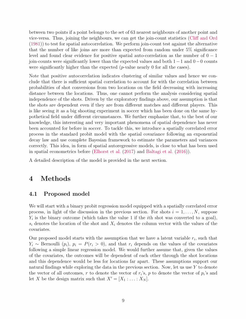
Recall that we can consider the occurrence of goals to be a spatial point process with the fieldbeing the location set. Plotting Ripley’s K-function (Dixon (2002)) is a standard techniqueto check whether there exists any spatial clustering or not. It is defined as K(a) = λ−1Ea

where λ is the density (number per unit area) of events (here goals), and Ea is the expectednumber of extra events within distance a of a randomly chosen event. In Figure 4, Ktheo(a),Khigh(a) and Klow(a) give us the expected values and confidence intervals of K(a) underthe assumption of spatial homogeneity and independence. We can clearly observe that theK(a) values diverge from the expected values indicating possible spatial correlation and morespatial clustering as a increases.

0.0 0.5 1.0 1.5 2.0 2.5 3.0

020

4060

Headers

a

K(a

)

Kobs(a)

Ktheo(a)

Khigh(a)

Klow(a)

0 2 4 6 8

010

020

030

040

050

060

0

Other Shots

a

K(a

)

Kobs(a)

Ktheo(a)

Khigh(a)

Klow(a)

Figure 4: Ripley’s K-functionK(a) is plotted against a for both headed and non-headed goalsconsidering goals as spatial point processes. Under spatial homogeneity and independence,K(a) = πa2. Expected values under this hypothesis and confidence intervals are constructedfor reference.

Now that we have a hint that there might be a spatial dependency involved, we test whetherthere exists spatial autocorrelation or not. We have a binary variable with 1 denoting a goaland 0 otherwise. We create a graph of the shot locations based on k-nearest neighbor criteriausing Euclidean distance (taking k = 63 as it has been accepted as a thumb rule to takek =

√n where n is the number of observations, here n = 3957,

√n ≈ 63). We join edges

8

between two points if a point belongs to the set of 63 nearest neighbours of another point andvice-versa. Thus, joining the neighbours, we can get the join-count statistics (Cliff and Ord(1981)) to test for spatial autocorrelation. We perform join-count test against the alternativethat the number of like joins are more than expected from random under 5% significancelevel and found clear evidence for positive spatial auto-correlation as the number of 0 − 1join-counts were significantly lower than the expected values and both 1−1 and 0−0 countswere significantly higher than the expected (p-value nearly 0 for all the cases).

Note that positive autocorrelation indicates clustering of similar values and hence we con-clude that there is sufficient spatial correlation to account for with the correlation betweenprobabilities of shot conversions from two locations on the field decreasing with increasingdistance between the locations. Thus, one cannot perform the analysis considering spatialindependence of the shots. Driven by the exploratory findings above, our assumption is thatthe shots are dependent even if they are from different matches and different players. Thisis like seeing it as a big shooting experiment in soccer which has been done on the same hy-pothetical field under different circumstances. We further emphasize that, to the best of ourknowledge, this interesting and very important phenomena of spatial dependence has neverbeen accounted for before in soccer. To tackle this, we introduce a spatially correlated errorprocess in the standard probit model with the spatial covariance following an exponentialdecay law and use complete Bayesian framework to estimate the parameters and variancescorrectly. This idea, in form of spatial autoregressive models, is close to what has been usedin spatial econometrics before (Elhorst et al. (2017) and Baltagi et al. (2016)).

A detailed description of the model is provided in the next section.

4 Methods

4.1 Proposed model

We will start with a binary probit regression model equipped with a spatially correlated errorprocess, in light of the discussion in the previous section. For shots i = 1, . . . , N , supposeYi is the binary outcome (which takes the value 1 if the ith shot was converted to a goal),si denotes the location of the shot and Xi denotes the column vector with the values of thecovariates.

Our proposed model starts with the assumption that we have a latent variable ri, such thatYi ∼ Bernoulli (pi), pi = P (ri > 0), and that ri depends on the values of the covariatesfollowing a simple linear regression model. We would further assume that, given the valuesof the covariates, the outcomes will be dependent of each other through the shot locationsand this dependence would be less for locations far apart. These assumptions support ournatural findings while exploring the data in the previous section. Now, let us use Y to denotethe vector of all outcomes, r to denote the vector of ri’s, p to denote the vector of pi’s andlet X be the design matrix such that X ′ = [X1 : . . . : XN ].

9

We are going to consider a hierarchical structure. First of all, Yi = I(ri > 0) and

ri = X ′

iθ + εi, (4.1)

where θ is a parameter vector of appropriate order, corresponding to the covariates and εiis the error process. Note that the mean function µi = X ′

iθ is considered to be an additivecombination of the effects of some continuous and some discrete covariates. We would furtherassume that the error process has the following structure:

εi = wi + ei. (4.2)

Here wi denotes a zero-mean spatially correlated process and ei stands for a zero-meanindependent and identically distributed (iid) white noise process. We assume that ei’s areiid N(0, σ2) while for wi’s, we take a correlation structure that decays exponentially. Inparticular, the covariance between wi and wj (i.e. for locations si and sj) is

Cov(wi, wj) = σ2

w exp(−φ ‖si − sj‖), (4.3)

where the distance function ‖si − sj‖ is taken as the Euclidean distance of the two locations.Writing w = (w1, . . . , wN), we will denote the covariance matrix of w by σ2

wΣw. Thus, wecan now write the full model in the following form:

Yi = I(ri > 0), (4.4)

r = Xθ + w + e,

such that w ∼ N(0, σ2

wΣw),

and e ∼ N(0, σ2I).

We are going to use a Bayesian framework to get estimates for the parameters in the model.For each of the components in the parameter vector θ, we will consider improper Jeffrey’sprior distribution. On the other hand, we will assume the two variance components σ2, σ2

w tobe equal. While we acknowledge the simplicity associated with this assumption, it is worthmentioning that we have performed some simulation studies and found that the performanceis approximately the same with the assumption. The prior we associate with σ2 is the inversegamma (IG) distribution with parameters a, b. We would take a > 1 to avoid improperposterior distributions.

And finally, the parameter φ (refer to Equation (4.3)) will be kept fixed throughout theBayesian analysis. Ideally, one should consider appropriate prior distribution and estimateit within the Bayesian model as well. But, simulation studies show that the computationalburden reduces to a great extent and the performance does not deteriorate if we keep itfixed and that motivated us to make this adjustment. In order to find out the best possiblevalue for φ, we would consider a cross-validation scheme. The possible choices for φ usedin the study were between 0.05 and 1. Based on the relationship e−φd ≈ 0.05, we chosethe above range, which corresponds to actual distances in the field ranging from 3 yards to60 yards. The validation scheme would consider prediction for 30% of all the shots after

10

estimating the parameters from the other 70% and would find out the mean squared errorfor those predictions. For shots considered for the validation purpose (let us denote themby i ∈ V = {v1, . . . , vm}), we would predict the probability of them being converted togoals and let the predicted probabilities be denoted by pi while Yi’s are the actual outcomes.Then, for each φ, we calculate the mean squared error of the predictions using the followingformula:

MSEφ =1

m

∑

i∈V

(Yi − pi)2. (4.5)

The value of φ with the least mean squared validation error will be our optimal choice forthe analysis. The prediction procedure is discussed in detail in Section 4.3.

4.2 Posterior distribution and Gibbs sampling

Throughout the discussion below, K will always indicate a constant term, that may varyfrom time to time. Using the full model described in Section 4.1 and the prior distribu-tions described in the paragraph following that equation, we can write the joint posteriordistribution as:

log π(r, θ, σ2, w |Y ) = K +N∑

i=1

{Yi log(P (ri > 0)) + (1− Yi) log(P (ri ≤ 0))} − b

σ2

−‖r −Xθ − w‖22σ2

− w′Σ−1

w w

2σ2− (a+N + 1) logσ2. (4.6)

Since simulating directly from the joint posterior distribution is difficult, we would use theprinciples of Gibbs sampling, which sequentially updates every parameter in an iterative wayuntil convergence. For σ2, we can get the full conditional distribution as:

log π(σ2 |Y, r, θ, w) = K − (a+N + 1) log σ2 − 1

σ2

[

b+1

2‖r −Xθ − w‖2 + 1

2w′Σ−1

w w

]

and thus,

(σ2 |Y, r, θ, w) ∼ IG

(

a+N, b+1

2‖r −Xθ − w‖2 + 1

2w′Σ−1

w w

)

. (4.7)

For θ, we get that

log π(θ |Y, r, σ2, w) = K − 1

2θ′(

X ′X

σ2

)

θ +1

2· 2θ′ · X

′(r − w)

σ2.

Straightforward calculations then tell us that the conditional posterior of θ is

(θ |Y, r, σ2, w) ∼ N(

(X ′X)−1X ′(r − w), σ2(X ′X)−1)

. (4.8)

11

On the other hand, using similar techniques as before, we can get the posterior distributionfor w as:

(w | Y, r, θ, σ2) ∼ N(

(I + Σ−1

w )−1(r −Xθ), σ2(I + Σ−1

w )−1)

. (4.9)

Note that the means of the conditional distributions of both θ and w require the computationof the products of a matrix and a vector, but the dispersion matrices of the same are updatedat every step only through the value of σ and so, one needs to compute the inverses of threebig matrices, namely X ′X , Σw and (I + Σ−1

w ), only once throughout the MCMC analysis.Hence, directly using the above conditional distribution of w at every step will not sufferfrom huge computational burden. However, one can always use component-wise conditionalposterior distributions to further increase the efficiency.

Finally, we find the conditional distribution of r. The joint posterior distribution in Sec-tion 4.2 clearly shows that conditional on data and other parameters, each component of r isindependent of others and simple calculations would reveal that the conditional distributionsare truncated normal as follows.

(ri |Y, θ, w, σ2) ∼{

TN(αi, σ2; 0,∞) if Yi = 1

TN(αi, σ2;−∞, 0) if Yi = 0

(4.10)

In the above, α = Xθ + w and TN(µ, τ 2; a, b) denotes a normal distribution with meanparameter µ and variance parameter τ 2, truncated in the interval [a, b].

4.3 Future prediction

In order to make a new prediction for a shot from location s′, we will take resort to theposterior estimates obtained from the Gibbs sampler. Let us denote the outcome of the shotfrom s′ by Y (s′) (X(s′), r(s′) and w(s′) are defined accordingly). Note that the posteriorpredictive distribution f(Y (s′) | Y ) can be written using an integral for the product of thedensity functions, where the integral is taken with respect to all the parameter vectors.However, instead of solving that integral, a better and more convenient idea is to use theGibbs sampler estimates to draw observations from the posterior predictive distribution andone can do it sequentially.

At first, we would draw samples for r, w, θ, σ2 using the conditional posterior distributionsdescribed in Section 4.2. After that, we would draw samples for w(s′) using the conditionaldistribution of (w(s′) |w, σ2) as discussed below. Using the above sampled observations, anestimate for r(s′) can be obtained by taking a sample from a normal distribution with meanX(s′)′θ + w(s′) and variance σ2. Finally, we set Y (s′) = I(r(s′) > 0). Alternately, one canalso use Y (s′) ∼ Bernoulli (p(s′)), where p(s′) = P (r(s′) > 0) can be computed using thesampled values of θ, σ2 and w(s′).

To compute the conditional distribution of (w(s′) |w, σ2), we start with the fact that

(

w(s′)w

)

∼ N

(

0, σ2

[

1 Σ′

s−s′

Σs−s′ Σw

])

.

12

Here, Σs−s′ is the column vector denoting the covariance of w(s′) with the elements of w.Following Equation (4.3), the jth element of Σs−s′ is exp(−φ ‖sj − s′‖). Using the principleof conditional distribution for multivariate normal distribution, we can then say that

w(s′) |w ∼ N(µnew, σ2

new), (4.11)

where σ2

new= σ2

(

1− (Σ′

s−s′Σ−1

w Σs−s′))

,

µnew = Σ′

s−s′Σ−1

w w.

4.4 Measures to quantify player abilities

Here, we propose two measures for rating a player’s scoring ability on the pitch based on ourmodel. To proceed, at first, we remove the shots taken by particular player of interest fromour data. This will be our training data to build the model and depending on the outputfrom this model, we will quantify each player in two ways, as described below.

To start with, we would like to introduce, what we call, the Shooting Prowess (SP) of aplayer. Suppose, in a total of gk matches, a player k has taken mk shots (calculated over atime period, possibly over a whole season or for the entire career) in total. The end resultof the ith shot, i = 1, . . . , mk, is denoted by Yi (0 for miss and 1 for goal) and the expectedprobability of the shot predicted from the training model is denoted by pi. Then, SV ki

(Shooting Value) of that shot is denoted by (Yi − pi). Note that this quantity lies in theinterval [−1, 1]; 1 denoting the best possible conversion and −1 denoting the worst miss.Using these shooting values for every shot, we define the measure SP k as follows:

SP k =1

gk

mk∑

i=1

SV ki =1

gk

mk∑

i=1

(Yi − pi) (4.12)

A discussion of why we put forward such a measure to quantify a player’s ability to scoregoals is warranted at this point. For any model to analyze such binary data, there are stillsome variances unaccounted for. It is a logical assumption that for a game like soccer, theconversion of a shot to goal will always depend on the player’s abilities. So, we suggest thatthe difference between the end result and the modeled probability of a shot being convertedto goal captures the shooter’s interference in that shot. On one hand, a high negative valuewill indicate a player missing a golden opportunity, thereby putting a negative impact onhis rating while on the other, successfully converting a shot with less theoretical probabilitywould capture the player’s more than average ability to score goals. The fact that wecalculate the average over the number of matches and not over the set of all shots capturesthe information of whether a player takes more shots in general. For example, a playertaking 2 shots in a match, with a SV of 0.5 each, will have lower ratings than another playerwho takes 10 shots in the same match, with a SV of 0.5 each, thereby proving that thesecond player is better and more consistent than the first player. A more sophisticated wayto quantify the SP is to consider a weighted average of the sum of shooting values per game,the weights being proportional to the number of minutes played in every match. Since wedid not have enough data on this, we chose to define it in the above fashion.

13

Next, we would like to quantify a player’s Positioning sense (PS), which is a pivotal thingfor a striker on the field in terms of scoring goals. One has to be at the right place at theright time to get a goal in his name. From our training model, we can estimate the shotconversion probability of an average player from a particular distance, angle and type ofopportunity. It is a different issue whether the player has grabbed the opportunity or not,but getting into a perfect position, he could ensure that a shot was fired. Hence, summingup the predicted probability of shot conversion for a particular player can give us a perfectidea about his positioning sense. Necessarily, the PSk (Positioning Sense) of the kth playeris defined by

PSk =1

gk

mk∑

i=1

pi. (4.13)

Once again, this measure captures the average effect per game and hence, has the aforemen-tioned nice property similar to the other measure.

5 Results

5.1 Fitting the model

Following the discussions in the previous sections, we consider two different models for ‘head-ers’ and ‘other shots’, and they can be written as follows.

For other shots, let Yi = I(ri > 0) denote whether ith shot was a goal. Then, we setri = µi + wi + ǫi, where wi, ǫi are as described in the previous section and µi is the meanfunction defined by

µi = β0 + β1 log(Di) + β2 cos(Ai) + β3Ki + β4Pi + β5I{Hi = 1}+ β6I{Fi = 1}

+

1∑

j=0

β7,jI{GDi = j}+ β8I{Si = 1}+3

∑

k=2

β9,jI{BPi = j}. (5.1)

Here, Di, Ai, Ki and Pi denote the continuous covariates, namely distance, angle, keepreachand proportion of shots converted against the same opponents. Indicators for Hi, Fi and Si

equal to 1 are used to denote if it was a home game, if it was in the first half and whether ithappened during stoppage time. GDi denotes whether the goal difference at the time of theshot was zero (j = 0) or positive (j = 1). And finally, BPi shows which body part (j = 1, 2, 3corresponding to other, left foot and right foot) was used in taking the shot. Note that wetake β7,−1 = β9,1 = 0 for identifiability purpose.

On the other hand, for ‘headers’, we do not consider the covariate BP , but the other modelremains unchanged.

Now, using the mean function (Section 5.1), we fit the model described in Section 4. Firstof all, using the procedure described towards the end of Section 4.1, we evaluate the best

14

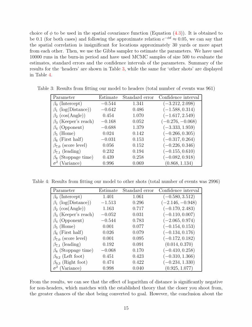
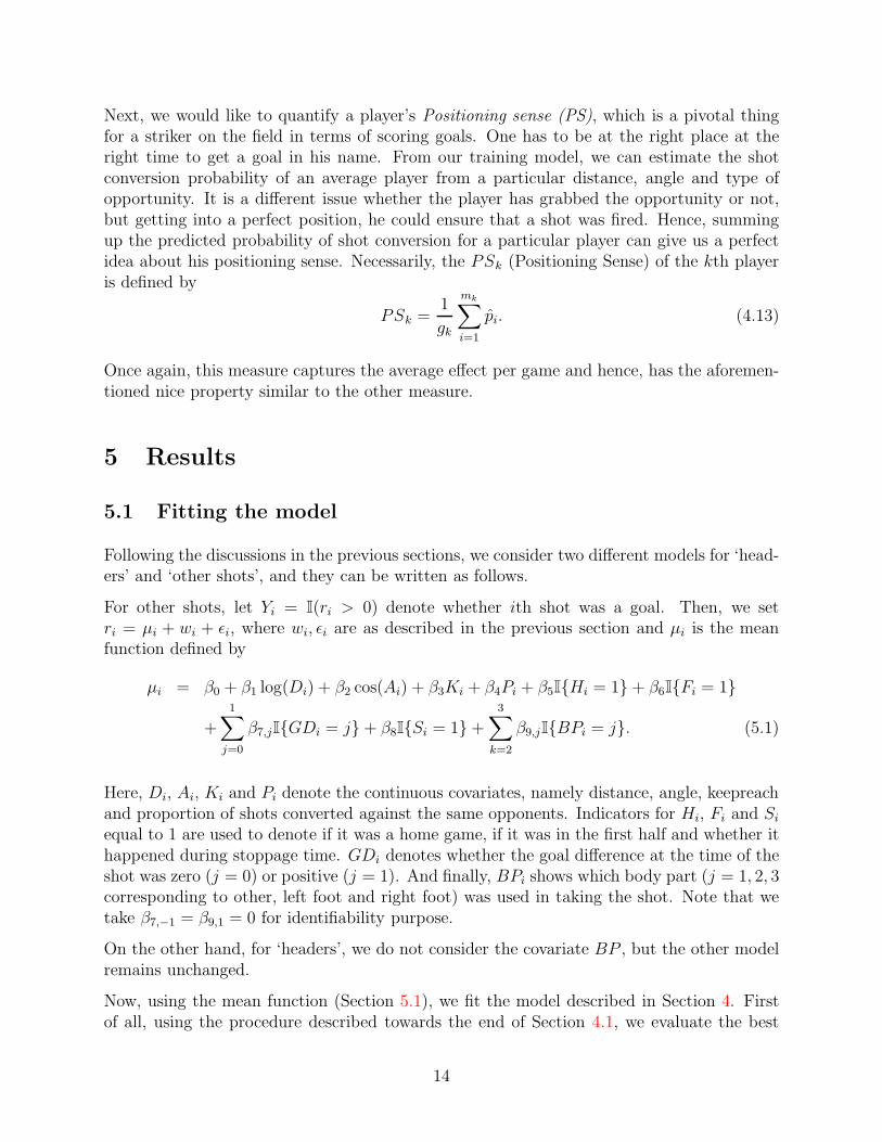
choice of φ to be used in the spatial covariance function (Equation (4.3)). It is obtained tobe 0.1 (for both cases) and following the approximate relation e−φd ≈ 0.05, we can say thatthe spatial correlation is insignificant for locations approximately 30 yards or more apartfrom each other. Then, we use the Gibbs sampler to estimate the parameters. We have used10000 runs in the burn-in period and have used MCMC samples of size 500 to evaluate theestimates, standard errors and the confidence intervals of the parameters. Summary of theresults for the ‘headers’ are shown in Table 3, while the same for ‘other shots’ are displayedin Table 4.

Table 3: Results from fitting our model to headers (total number of events was 961)

Parameter Estimate Standard error Confidence intervalβ0 (Intercept) −0.544 1.341 (−3.212, 2.098)β1 (log(Distance)) −0.642 0.486 (−1.588, 0.314)β2 (cos(Angle)) 0.454 1.070 (−1.617, 2.549)β3 (Keeper’s reach) −0.168 0.052 (−0.276,−0.068)β4 (Opponent) −0.688 1.379 (−3.333, 1.959)β5 (Home) 0.024 0.142 (−0.266, 0.305)β6 (First half) −0.031 0.153 (−0.317, 0.264)β7,0 (score level) 0.056 0.152 (−0.226, 0.346)β7,1 (leading) 0.232 0.194 (−0.155, 0.610)β8 (Stoppage time) 0.439 0.258 (−0.082, 0.918)σ2 (Variance) 0.996 0.069 (0.868, 1.134)

Table 4: Results from fitting our model to other shots (total number of events was 2996)

Parameter Estimate Standard error Confidence intervalβ0 (Intercept) 1.401 1.061 (−0.580, 3.512)β1 (log(Distance)) −1.513 0.296 (−2.146,−0.948)β2 (cos(Angle)) 1.163 0.717 (−0.170, 2.483)β3 (Keeper’s reach) −0.052 0.031 (−0.110, 0.007)β4 (Opponent) −0.544 0.783 (−2.065, 0.974)β5 (Home) 0.001 0.077 (−0.154, 0.153)β6 (First half) 0.026 0.079 (−0.134, 0.176)β7,0 (score level) 0.001 0.095 (−0.172, 0.182)β7,1 (leading) 0.192 0.091 (0.014, 0.370)β8 (Stoppage time) −0.068 0.170 (−0.410, 0.258)β9,2 (Left foot) 0.451 0.423 (−0.310, 1.366)β9,3 (Right foot) 0.474 0.422 (−0.234, 1.330)σ2 (Variance) 0.998 0.040 (0.925, 1.077)

From the results, we can see that the effect of logarithm of distance is significantly negativefor non-headers, which matches with the established theory that the closer you shoot from,the greater chances of the shot being converted to goal. However, the conclusion about the

15

‘angle’ of shots is interesting. While in the simple logistic regression model used by currentresearchers in this field, it was found that a smaller angle (higher value of the cosine of theangles) significantly increases the goal-scoring chance, we have found that the angle of theshot is not a significant variable in our model. This happens probably because the effect ofthe angle is already being explained by the spatial process.

For headers, however, neither the distance nor the angle is significant. In fact, no othercovariate except keeper’s reach is significant for headers. The chance of converting froma header increases when the keeper’s reach is less. But, barring that, it is clear that theinclusion of the spatially correlated process can explain most of the variability in the data.

Further, for non-headed shots, so far as the other covariates are concerned, we can see thatthe chances increase significantly when the shooter’s team leads. It is in line with the notionthat a positive goal difference can boost the morale of the team to a great extent. However,we observed that the opponent effect, the home advantage, the half or the stoppage time doesnot play a significant role in explaining the shot conversion rates. The conclusion is samefor left or right footed shots, though it is worth noting that the coefficients corresponding tothese two covariates are very close to each other (0.451 and 0.474), thereby supporting thenature of symmetry in the game of soccer.

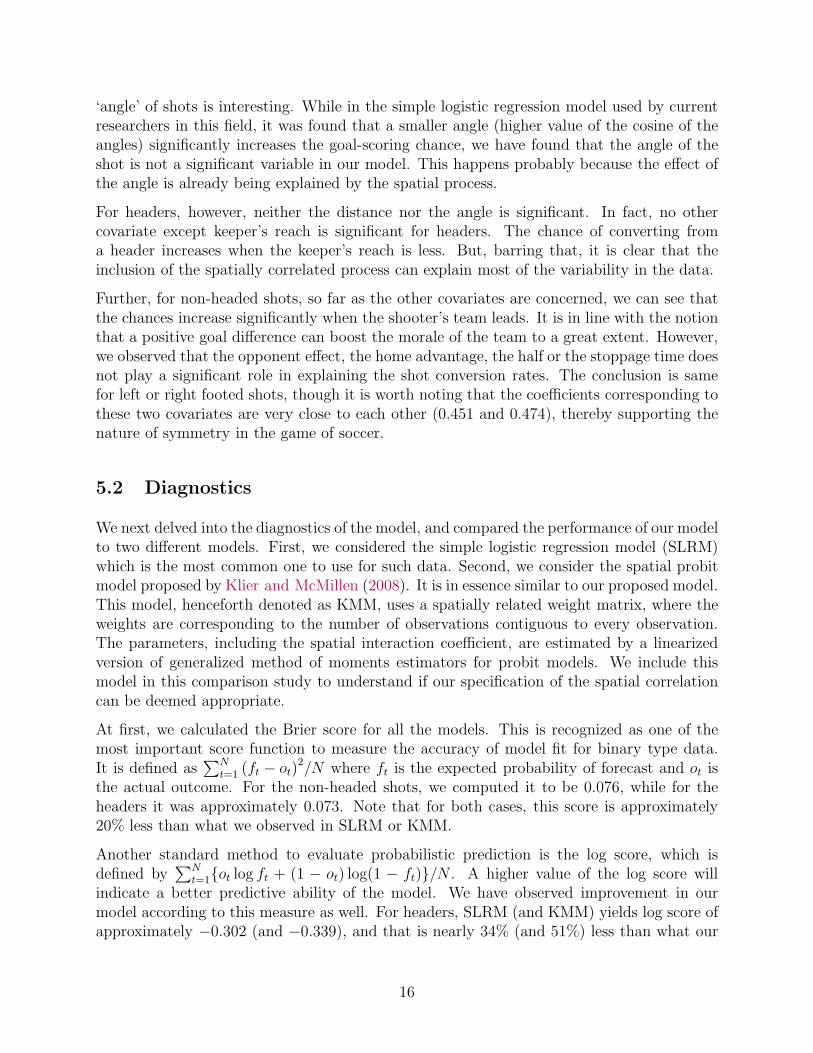
5.2 Diagnostics

We next delved into the diagnostics of the model, and compared the performance of our modelto two different models. First, we considered the simple logistic regression model (SLRM)which is the most common one to use for such data. Second, we consider the spatial probitmodel proposed by Klier and McMillen (2008). It is in essence similar to our proposed model.This model, henceforth denoted as KMM, uses a spatially related weight matrix, where theweights are corresponding to the number of observations contiguous to every observation.The parameters, including the spatial interaction coefficient, are estimated by a linearizedversion of generalized method of moments estimators for probit models. We include thismodel in this comparison study to understand if our specification of the spatial correlationcan be deemed appropriate.

At first, we calculated the Brier score for all the models. This is recognized as one of themost important score function to measure the accuracy of model fit for binary type data.It is defined as

∑N

t=1(ft − ot)

2/N where ft is the expected probability of forecast and ot isthe actual outcome. For the non-headed shots, we computed it to be 0.076, while for theheaders it was approximately 0.073. Note that for both cases, this score is approximately20% less than what we observed in SLRM or KMM.

Another standard method to evaluate probabilistic prediction is the log score, which isdefined by

∑N

t=1{ot log ft + (1 − ot) log(1 − ft)}/N . A higher value of the log score will

indicate a better predictive ability of the model. We have observed improvement in ourmodel according to this measure as well. For headers, SLRM (and KMM) yields log score ofapproximately −0.302 (and −0.339), and that is nearly 34% (and 51%) less than what our

16

method gives (log score of about −0.225). Similar phenomena was observed for non-headedshots as well.

Next, we evaluated the proportion of times the models could classify the outcomes correctly.Here, the improvement with our model was only about 10%, as compared to SLRM or KMM.

The above results are summarized in table 5.

Table 5: Comparison of three candidate models

SLRM KMM Our modelBrier Score 0.091 0.101 0.073

Headers log score −301.738 −338.876 −224.735error % 11.03% 11.654% 10.406%Brier Score 0.094 0.098 0.076

Other shots log score −958.212 −1043.567 −728.228error % 11.983% 11.983% 10.748%

As a final piece, we wanted to see how accurately we can predict outcomes based on themodel we developed. At this point, one should keep in mind that this is a case of rare eventsbinary regression and one of the main issues with these scenarios is that the predictionproblem is immensely difficult and some calibration method is always needed, which furtherrequires more information on the whole population, as pointed out by King and Zeng (2001).Since we did not have that information, we had to rely on usual prediction methods (refer toSection 4.3). We used cross-validation techniques to evaluate how good the predictions are,by taking a subset of the full data (approximately 90%) to learn the model and applying iton the rest (approximately 10%). Afterwards, in order to evaluate the prediction efficiency,we followed the general scoring rules outlined by Merkle and Steyvers (2013).

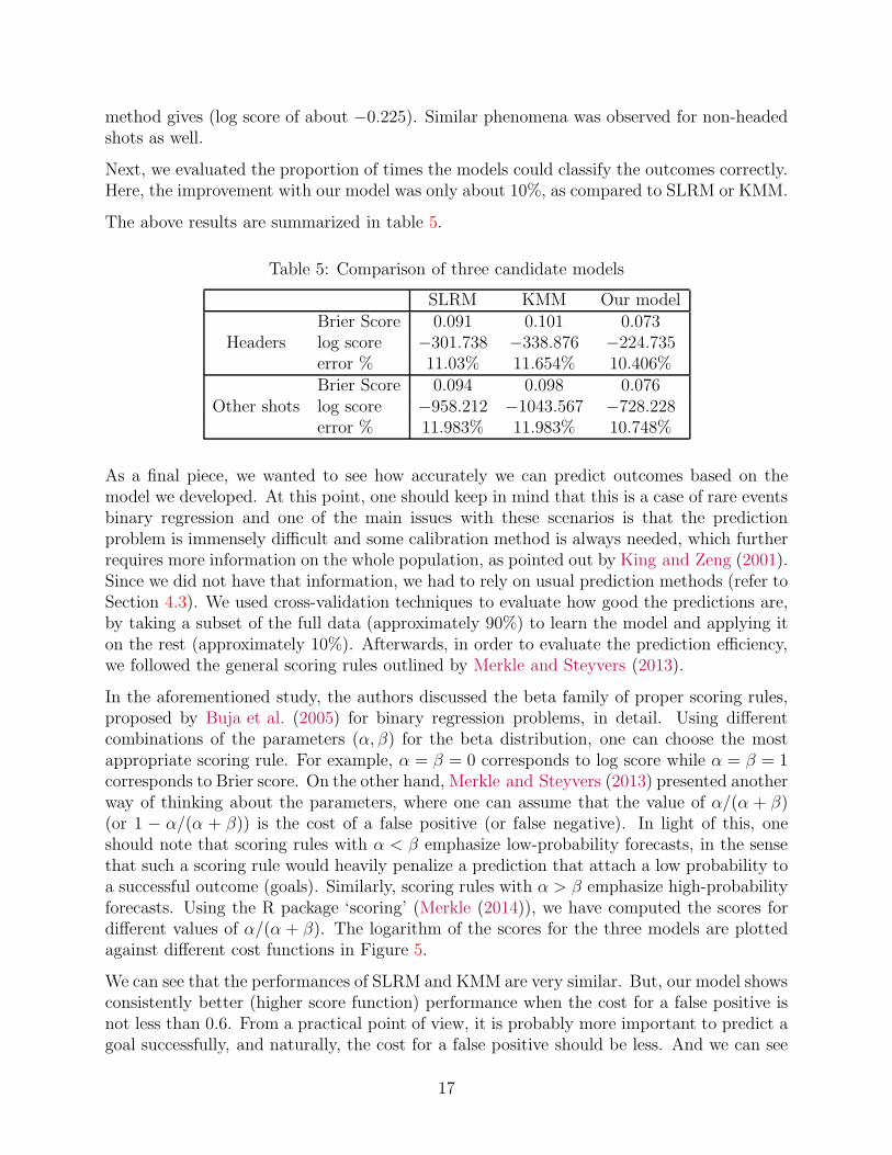
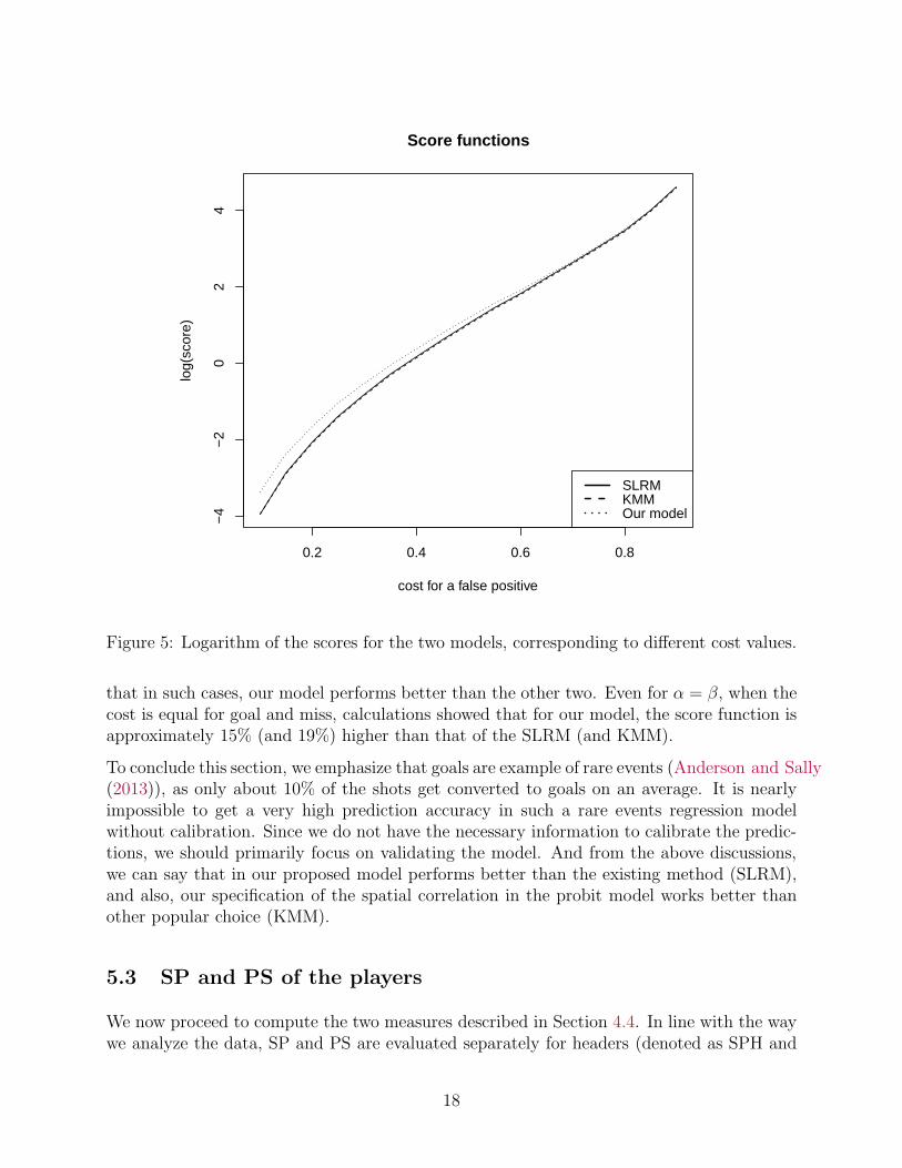
In the aforementioned study, the authors discussed the beta family of proper scoring rules,proposed by Buja et al. (2005) for binary regression problems, in detail. Using differentcombinations of the parameters (α, β) for the beta distribution, one can choose the mostappropriate scoring rule. For example, α = β = 0 corresponds to log score while α = β = 1corresponds to Brier score. On the other hand, Merkle and Steyvers (2013) presented anotherway of thinking about the parameters, where one can assume that the value of α/(α + β)(or 1 − α/(α + β)) is the cost of a false positive (or false negative). In light of this, oneshould note that scoring rules with α < β emphasize low-probability forecasts, in the sensethat such a scoring rule would heavily penalize a prediction that attach a low probability toa successful outcome (goals). Similarly, scoring rules with α > β emphasize high-probabilityforecasts. Using the R package ‘scoring’ (Merkle (2014)), we have computed the scores fordifferent values of α/(α + β). The logarithm of the scores for the three models are plottedagainst different cost functions in Figure 5.

We can see that the performances of SLRM and KMM are very similar. But, our model showsconsistently better (higher score function) performance when the cost for a false positive isnot less than 0.6. From a practical point of view, it is probably more important to predict agoal successfully, and naturally, the cost for a false positive should be less. And we can see

17

0.2 0.4 0.6 0.8

−4

−2

02

4

Score functions

cost for a false positive

log(

scor

e)

SLRMKMMOur model

Figure 5: Logarithm of the scores for the two models, corresponding to different cost values.

that in such cases, our model performs better than the other two. Even for α = β, when thecost is equal for goal and miss, calculations showed that for our model, the score function isapproximately 15% (and 19%) higher than that of the SLRM (and KMM).

To conclude this section, we emphasize that goals are example of rare events (Anderson and Sally(2013)), as only about 10% of the shots get converted to goals on an average. It is nearlyimpossible to get a very high prediction accuracy in such a rare events regression modelwithout calibration. Since we do not have the necessary information to calibrate the predic-tions, we should primarily focus on validating the model. And from the above discussions,we can say that in our proposed model performs better than the existing method (SLRM),and also, our specification of the spatial correlation in the probit model works better thanother popular choice (KMM).

5.3 SP and PS of the players

We now proceed to compute the two measures described in Section 4.4. In line with the waywe analyze the data, SP and PS are evaluated separately for headers (denoted as SPH and

18

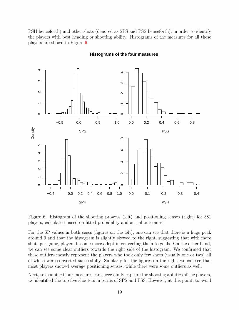
PSH henceforth) and other shots (denoted as SPS and PSS henceforth), in order to identifythe players with best heading or shooting ability. Histograms of the measures for all theseplayers are shown in Figure 6.

SPS

−0.5 0.0 0.5 1.0

01

23

4

PSS

0.0 0.2 0.4 0.6 0.80

12

34

SPH

−0.4 0.0 0.2 0.4 0.6 0.8 1.0

01

23

45

PSH

0.0 0.1 0.2 0.3 0.4

02

46

8

Histograms of the four measures

Den

sity

Figure 6: Histogram of the shooting prowess (left) and positioning senses (right) for 381players, calculated based on fitted probability and actual outcomes.

For the SP values in both cases (figures on the left), one can see that there is a huge peakaround 0 and that the histogram is slightly skewed to the right, suggesting that with moreshots per game, players become more adept in converting them to goals. On the other hand,we can see some clear outliers towards the right side of the histogram. We confirmed thatthese outliers mostly represent the players who took only few shots (usually one or two) allof which were converted successfully. Similarly for the figures on the right, we can see thatmost players showed average positioning senses, while there were some outliers as well.

Next, to examine if our measures can successfully capture the shooting abilities of the players,we identified the top five shooters in terms of SPS and PSS. However, at this point, to avoid

19

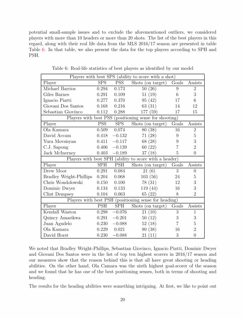
potential small-sample issues and to exclude the aforementioned outliers, we consideredplayers with more than 10 headers or more than 20 shots. The list of the best players in thisregard, along with their real life data from the MLS 2016/17 season are presented in tableTable 6. In that table, we also present the data for the top players according to SPH andPSH.

Table 6: Real-life statistics of best players as identified by our model

Players with best SPS (ability to score with a shot)Player SPS PSS Shots (on target) Goals AssistsMichael Barrios 0.294 0.173 50 (26) 9 2Giles Barnes 0.291 0.109 51 (19) 6 3Ignacio Piatti 0.277 0.370 95 (42) 17 6Giovani Dos Santos 0.168 0.216 63 (31) 14 12Sebastian Giovinco 0.112 0.288 177 (59) 17 15

Players with best PSS (positioning sense for shooting)Player PSS SPS Shots (on target) Goals AssistsOla Kamara 0.509 0.074 80 (38) 16 2David Accam 0.418 −0.132 71 (28) 9 5Yura Movsisyan 0.411 −0.117 68 (28) 9 3C.J. Sapong 0.406 −0.139 60 (22) 7 2Jack McInerney 0.403 −0.189 37 (18) 5 0

Players with best SPH (ability to score with a header)Player SPH PSH Shots (on target) Goals AssistsDrew Moor 0.291 0.084 21 (6) 3 0Bradley Wright-Phillips 0.204 0.068 103 (56) 24 5Chris Wondolowski 0.150 0.100 78 (31) 12 3Dominic Dwyer 0.134 0.133 119 (44) 16 3Clint Dempsey 0.104 0.063 65 (22) 8 2

Players with best PSH (positioning sense for heading)Player PSH SPH Shots (on target) Goals AssistsKendall Waston 0.298 −0.076 21 (10) 3 1Quincy Amarikwa 0.291 −0.201 50 (12) 3 3Juan Agudelo 0.230 −0.088 52 (18) 7 5Ola Kamara 0.229 0.021 80 (38) 16 2David Horst 0.230 −0.088 21 (11) 3 0

We noted that Bradley Wright-Phillips, Sebastian Giovinco, Ignacio Piatti, Dominic Dwyerand Giovani Dos Santos were in the list of top ten highest scorers in 2016/17 season andour measures show that the reason behind this is that all have great shooting or headingabilities. On the other hand, Ola Camara was the sixth highest goal-scorer of the seasonand we found that he has one of the best positioning senses, both in terms of shooting andheading.

The results for the heading abilities were something intriguing. At first, we like to point out

20

the special cases of Drew Moor, Kendall Waston and David Horst. All of them are defendersand their heading abilities are supposed to be good. In soccer, it is often observed that thedefenders move ahead during a corner or a long free-kick. Naturally, it would be beneficial forthe teams to identify which defenders can take good positions during the set-piece situationsand convert the chances that come in the way. It is evident that our model can serve thatpurpose well. On the other hand, Juan Agudelo and Quincy Amarikwa showed really goodpositioning senses when it comes to heading. But, their conversion abilities are poor andthat has affected their overall stats. In fact, they were also not the first choice strikers oftheir respective teams. Finally, we note that Clint Dempsey, one of the finest players UnitedStates of America has ever produced, has brilliant heading prowess, but his SP quotient wasnot one of the best in the league.

It is worth mention here that the training data we used in our model contained informationonly from a part of the season and the above measures are always calculated based on otherplayers’ data. Thus, it is interesting that the list of best players according to these measuresconsists mostly of the players who were actually at the top of the goal-scoring chart afterthe season ended. This clearly reflects that we have been able to single out the players’goal-scoring abilities and positioning senses perfectly. In real life, it has huge potential toidentify most suitable players in different scenarios.

6 Summary

In conclusion, we have presented an alternate way of analyzing the conversion rate of shotsin soccer. Using a spatially correlated error process, we have shown that our model fits thedata well. Our proposed method has exhibited improved Brier score, log score and predictiveabilities, as compared to the logistic regression model that is in practice at the moment. Onthe other hand, our way of specifying the spatial correlation term is also more appropriatethan other possible way for probit regression models. Another key contribution of our workis to properly quantify the shooters’ efficiency and positioning sense. To the best of ourknowledge, this is the first paper to introduce such measures. We have also established thatthe quantitative measures are good enough to identify the best strikers and thus, the teamswould certainly be benefited from using this concept. In a more specialized way, conditioningon different opponents, one can use relevant data to find out the best shooters against themand that would help the coaches in making strategies and tactics against particular teams.

On a related note, we also mention that using a similar measure for the goalkeepers, one canquantify the ‘saving prowess’ to single out the best custodians in the league. We chose notto do that in this study, for we think the goalkeepers’ abilities should not be evaluated solelybased on the number of goals conceded, but also on the number of blocks and saves made bythe goalkeeper. And that is one of the future directions we are interested in. We emphasizethat the methods we described here are applicable to binary data (goals and misses), butit can be extended to the multinomial case (blocked, goal, missed, hit by post or saved) aswell and that is what needs to be done to identify the best goalkeepers in business.

A minor issue with our model is that if we have the exact same co-ordinates for two shot

21

locations, then the covariance matrix associated with the error process will be singular andthe model will fail. But, theoretically, it is a measure zero event and it happens very rarelyin practice. For example, we did not encounter such an issue in our data. To understand it abit further, observe that penalty kicks are one such kind of events, where the shots are takenfrom a fixed location inside the box. But, penalty kicks should not be considered in a studylike ours because the outcome of the spot-kicks do not really depend on the distance, angleor other physiological attributes. Rather, it only depends on the penalty taker’s abilities andusually every team has a specialist for this job. Hence, quite rightly, we left out these casesfrom the data before running the analysis. Now, apart from penalty kicks, even if we havetwo or more shots fired from the same exact location, we can easily make adjustments asfollows. Suppose, z1, .., zk are the shots fired from exact same location. Then, we randomlypick one shot from z1, .., zk and leave out the other shots from the data. Next, we fit themodel based on the available data and predict the outcomes of the left-out shots from themodel. We calculate the sum of squared prediction errors in this case and continue thisprocedure for all of the k shots. And finally, we pick the shot with the lowest error andinclude it, discarding the rest, in our final model.

We also note that the parameter φ (refer to Equation (4.3)), which denotes the extentof spatial dependence, is not estimated directly from our model. Instead, we use a cross-validation approach to find out the best choice of φ from a grid. Naturally, this does not allowus to test the hypothesis of no spatial dependence, cf. Anselin (2001). While it might seema disadvantage, we want to point out that this is a common practice in many spatial studies,see, for example, Sahu et al. (2006). In fact, in this study, we built the model after gettingsufficient evidence in favour of spatial autocorrelation and hence, afterwards, we are moreinterested in explaining the variation among conversion of shots explained by the covariatesand the spatial error process and then, how accurately we can predict the outcomes. Theresults establish that our model works well to serve that purpose.

Finally, we believe that we could have improved the predictions if we had more intensedata containing information like the shot speed, the attacking speed and the position of thedefenders in the shooting range of the shooter. As our model is really flexible, in future,we aim to incorporate those attributes in the discussion to conduct a more comprehensivestudy.

7 Acknowledgement

We thank Dr. Chris Anderson, the author of The Numbers Game : Why Everything YouKnow About Soccer Is Wrong and a pioneer in soccer analytics, for providing his valuablefeedback about our approach to address the research problem. Our gratefulness also goes toAmerican Soccer Analysis (ASA) for providing the data in this study.

22

References

American Soccer Analysis (2016), ‘Expected goals 2016 - xgoals explanation’.URL: http://www.americansocceranalysis.com/explanation/

Anderson, C. and Sally, D. (2013), The numbers game: Why everything you know aboutsoccer is wrong, Penguin.

Anselin, L. (2001), ‘Rao’s score test in spatial econometrics’, Journal of statistical planningand inference 97(1), 113–139.

Baltagi, B., LeSage, J. and Pace, R. (2016), Spatial Econometrics: Qualitative and LimitedDependent Variables, Advances in econometrics, Emerald Publishing Limited.URL: https://books.google.com/books?id=O4K9jwEACAAJ

Bertin, M. (2015), ‘Why soccer’s most popular advanced stat kind of sucks’, Deadspin .URL: http://bit.ly/2qtKK3E

Brooks, J., Kerr, M. and Guttag, J. (2016), ‘Using machine learning to draw inferencesfrom pass location data in soccer’, Statistical Analysis and Data Mining: The ASA DataScience Journal 9(5), 338–349.

Buja, A., Stuetzle, W. and Shen, Y. (2005), ‘Loss functions for binary class probabilityestimation and classification: Structure and applications’, Working draft, November .

Clark, T., Johnson, A. and Stimpson, A. (2013), Going for three: Predicting the likelihood offield goal success with logistic regression, in ‘The 7th Annual MIT Sloan Sports AnalyticsConference’.

Cliff, A. D. and Ord, J. K. (1981), Spatial processes: models & applications, Taylor & Francis.

Dixon, P. M. (2002), ‘Ripley’s k function’, Encyclopedia of environmetrics .

Elhorst, J. P., Heijnen, P., Samarina, A. and Jacobs, J. P. (2017), ‘Transitions at differentmoments in time: A spatial probit approach’, Journal of Applied Econometrics 32(2), 422–439.

Goddard, J. (2005), ‘Regression models for forecasting goals and match results in associationfootball’, International Journal of forecasting 21(2), 331–340.

Hughes, M. and Franks, I. (2005), ‘Analysis of passing sequences, shots and goals in soccer’,Journal of Sports Sciences 23(5), 509–514.

Jordet, G., Bloomfield, J. and Heijmerikx, J. (2013), The hidden foundation of field visionin english premier league (epl) soccer players, in ‘Proceedings of the MIT Sloan SportsAnalytics Conference’.

King, G. and Zeng, L. (2001), ‘Logistic regression in rare events data’, Political analysis9(2), 137–163.

Klier, T. and McMillen, D. P. (2008), ‘Clustering of auto supplier plants in the united states:

23

generalized method of moments spatial logit for large samples’, Journal of Business &Economic Statistics 26(4), 460–471.

Lasek, J., Szlavik, Z. and Bhulai, S. (2013), ‘The predictive power of ranking systems inassociation football’, International Journal of Applied Pattern Recognition 1(1), 27–46.

Leitner, C., Zeileis, A. and Hornik, K. (2010), ‘Forecasting sports tournaments by ratingsof (prob) abilities: A comparison for the euro 2008’, International Journal of Forecasting26(3), 471–481.

Lucey, P., Bialkowski, A., Monfort, M., Carr, P. and Matthews, I. (2014), Quality vs quan-tity: Improved shot prediction in soccer using strategic features from spatiotemporal data,in ‘Proc. 8th Annual MIT Sloan Sports Analytics Conference’, pp. 1–9.

Merkle, E. (2014), scoring: Proper scoring rules. R package version 0.5-1.URL: https://CRAN.R-project.org/package=scoring

Merkle, E. C. and Steyvers, M. (2013), ‘Choosing a strictly proper scoring rule’, DecisionAnalysis 10(4), 292–304.

Moura, F. A., Santiago, P. R. P., Misuta, M. S., de Barros, R. M. L. and Cunha, S. A. (2007),Analysis of the shots to goal strategies of first division brazilian professional soccer teams,in ‘ISBS-Conference Proceedings Archive’, Vol. 1.

Sahu, S. K., Gelfand, A. E. and Holland, D. M. (2006), ‘Spatio-temporal modeling offine particulate matter’, Journal of Agricultural, Biological, and Environmental Statistics11(1), 61–86.

Williams, T. and Walters, C. (2011), The effects of altitude on soccer match outcomes, in‘Proceedings of the MIT Sloan Sports Analytics Conference’.

24