spaceborne polarimeteric synthetic aperture...
TRANSCRIPT

1
SPACEBORNE POLARIMETERIC SYNTHETIC APERTURE RADAR
Università di Roma Tor VergataDipartimento di Ingegneria Civile e Ingegneria Informatica - DICII
GEOINFORMATION PHD

2
I – Spaceborne Polarimetric Synthetic Aperture Radars
II – Polarization Diversity
III – Polarimetric FeaturesIII – Polarimetric Features
IV - Applications
V - Software
Index
VI - Conclusions

3
SECTION I
Spaceborne Polarimetric Synthetic Aperture Radars

4
Polarimetric SAR systemsPolarimetric SAR systems
Generic polarimetric radar system

5
Multipolarization SystemsMultipolarization Systems- Incoherent systems –
No info about relative phase between orthogonal polarization channels
Can not derive Stokes vector of received field
● Same PRF as Single Pol● Halved azimuth resolution● One Receiving Channel at a time

6
Dual Polarimetric SystemsDual Polarimetric Systems
- Coherent systems –Has info about relative phase between
orthogonal polarization channels
● Same PRF as Single Pol● Same azimuth resolution● Two Receiving Channels
● Doubled PRF with respect to Single Pol
● Reduced range swath (avoid ambiguities)
● One Receiving Channel at a time

7
Full Polarimetric SystemsFull Polarimetric Systems
- Quad Pol systems –Collect all polarimetric information
S matrix
● Doubled PRF with respect to Single Pol● Reduced range swath (avoid ambiguities)● Two Receiving Channels

8
Calibration and CrosstalkCalibration and Crosstalk
[OHH OHV
OVH OVV]=[RHH RHV
RVH RVV ][PHH PHVPVH PVV ][
S HH S HVSVH SVV ][
PHH PHVPVH PVV ][
T HH T HVT VH TVV ]+[
N HH N HV
N VH N VV]
O=R P S PT+NGeneral Model
ScatteringMatrix
Propagationeffects
DistortionEffects on
RX
DistortionEffects on
TX
NoiseObserved
Matrix

9
Calibration and CrosstalkCalibration and Crosstalk
P=[1 00 1]
Propagationeffects
DistortionEffects on RX
DistortionEffects on TX
R=[ 1 δ2δ1 f 1] T=[1 δ4
δ3 f 2]
Channel imbalances
δ1 δ2 δ3 δ4
CrossTalk
On receive On transmit
f 1 f 2Limited by transmitting equal power on both
channels
Special correction techniques required
O=R S T

10
Compact PolarimetryCompact Polarimetry
Reasonable strategy when full polarimetry is precluded
TRANSMIT ONE POLARIZATION RECEIVE TWO ORTHOGONAL POLARIZATIONS
Advantages
Simpler space segment
Lower amount of transmitted data
Can retrieve Stokes vector of the received field
Azimuth resolution not halved
Less risk of crosstalk

11
Compact Polarimetry ModesCompact Polarimetry Modes
45°
H
V
H
V
L L
LR
TX
RX
Circular TransmitLinear Receive
Dual CircularPolarimetricΠ/4
12
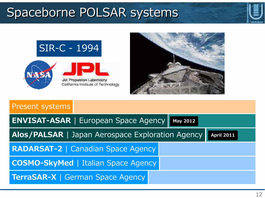
Spaceborne POLSAR systemsSpaceborne POLSAR systems
SIR-C - 1994
Present systems
ENVISAT-ASAR | European Space Agency
Alos/PALSAR | Japan Aerospace Exploration Agency
RADARSAT-2 | Canadian Space Agency
COSMO-SkyMed | Italian Space Agency
TerraSAR-X | German Space Agency
May 2012
April 2011

13
PresentPresent
ENVISAT-ASAR – 2002
Nominal Height Revisit Time Inclination
785 km 35 days 98,6°
Image Mode Polarization Mode Swath Spatial Resolution
Imaging, Wave, Alternating Single, AP 100 km 9 – 150 m
Radar Frequency Incidence Angle Polarizations Bandwidth
5,3 Ghz (C-band) 15° - 45° HH,HV,VH,VV N/A

14
PresentPresent
Alos/PALSAR - 2006
Nominal Height Revisit Time Inclination
691,65 km 46 days 98,16°
Image Mode Polarization Mode Swath Spatial Resolution
Fine, ScanSAR, Polarimetric Single, Dual, Quad 40-70 Km 14-88 m
Radar Frequency Incidence Angle Polarizations Bandwidth
1,27 Ghz (L-band) 8° - 60° HH,HV,VH,VV 14 – 28 MHz

15
PresentPresent
Radarsat-2 – 2007
Nominal Height Revisit Time Inclination
546 km 11 days 97°
Radar Frequency Incidence Angle Polarizations PRF
5,32 GHz 20° - 55° HH,HV,VV 3500 Hz
Nominal Height Revisit Time Inclination
798 km 24 days 98,6°
Image Mode Polarization Mode Swath Spatial Resolution
Fine, Standard, ScanSAR, Quad Single, Dual, Quad 50-500 km 10 – 100 m
Radar Frequency Incidence Angle Polarizations Bandwidth
5,40 Ghz (C-band) 20° - 40° HH,HV,VH,VV 100 MHz

16
PresentPresent
COSMO-SkyMed - 2007
Nominal Height Revisit Time Inclination
619 km 12 hours 97,86°
Image Mode Polarization Mode Swath Spatial Resolution
StripMap, ScanSAR, Spotlight Single, PingPong 10 – 200 km 1 – 30 m
Radar Frequency Incidence Angle Polarizations Bandwidth
9,6 Ghz (X-band) 20° - 59° HH, VV, VH, HV 400 MHz

17
PresentPresent
TerraSAR-X - 2007
Nominal Height Revisit Time Inclination
514 km 11 days 97,44°
Image Mode Polarization Mode Swath Spatial Resolution
StripMap, ScanSAR, Spotlight Single, Dual, Quad (experimental)
30 - 15 Km 1 - 18 m
Radar Frequency Incidence Angle Polarizations Bandwidth
9,65 Ghz (X-band) 20° - 45° HH,HV,VH,VV 150 – 300 MHz

18
FutureFuture
Sentinel-1 - 2013
Constellation of two satellite – Revisit Time 1-3 days
Continuity of C-band ESA commitment [ERS-1/2, ENVISAT]
Single or Dual Polarimetric Imaging Modes
Constellation of two satellite – Revisit Time 1-3 days
Continuity of C-band ESA commitment [ERS-1/2, ENVISAT]
Single or Dual Polarimetric Imaging Modes
Resolutions 5 to 40 m | Swath width 80 to 400 km

19
FutureFuture
Alos-2 - 2013
Improved NESZ, Resolution, Signal-To-Ambiguity Ratio
Follow on of Alos Mission (L-band)
Single, Dual, Full and Compact Polarimetric Modes
Resolutions 1 to 100 m | Swath width 50 to 500 km

20
FutureFuture
Radarsat Constellation – 2014/2015
Constellation of three C-band medium resolution satellites
Follow on of Radarsat-2 mission
Single, Dual, Quad and Compact polarimetric modes
Resolutions 3 to 100 m | Swath width 20 to 500 km

21
FutureFuture
SAOCOM – 2015/2016
Part of SIASGE program with ASI
Two L-band full polarimetric satellites – 8 days repeat cycle
StripMap and TOPSAR and CTLR CP Imaging Modes
Resolutions 10 to 100 m | Swath width 40 to 350 km

22
FutureFuture
COSMO SkyMed Seconda Generazione - 2014/2015
Complete integration with COSMO-SkyMed - CSK
Ensured continuity of X-band ASI commitment
Single or Dual Polarimetric Imaging Modes
Along Track Interferometry Mode (ATI)
Improved Resolution (500 Mhz Bandwitdh)
Experimental Quad Polarimetric Mode

23
SECTION II
Polarization Diversity

24
E (r , t )=ℜ{E (r )e jω t}
Wave Polarization – The Jones formalismWave Polarization – The Jones formalism
E (r )=E 0 e− j k⋅rPlane wave propagating along z
axis from the source in a lossless homogeneous medium.
E 0 Complex Amplitude k Wave vector
Monocromatic Time-SpaceElectric field
E (r , t )=[E0x cos(ω t−k z+δ x)
E0ycos(ω t−k z+δ y)]=ℜ{[E0x ej δx
E0y ej δy]e− j k z e− jω t}
Jones VectorE

25
Wave Polarization – The Jones formalismWave Polarization – The Jones formalism
Right Circular
VerticalHorizontal
Left Circular
EH=[10] EV=[01]
ER=1
√2 [1− j] EL=
1
√2 [1j]

26
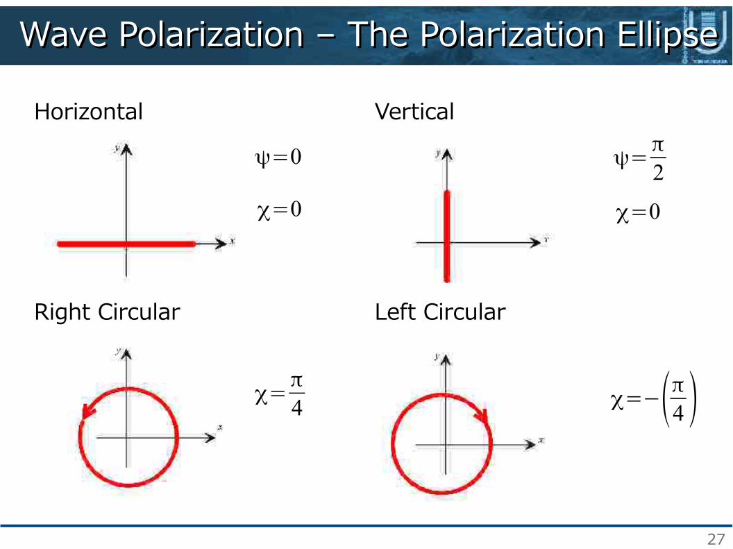
Wave Polarization – The Polarization EllipseWave Polarization – The Polarization Ellipse
E 0xE 0y
=tan (α)
δ=δ x−δy
ψ=(tan (2α)cos (δ)2 )
χ=arcsin (sin (2α)sin (δ)2 )
Rotation angle
Ellipticity
PolarizationEllipse
27
ψ=π
2
χ=0
χ=−(π4 )
Wave Polarization – The Polarization EllipseWave Polarization – The Polarization Ellipse
Right Circular
VerticalHorizontal
Left Circular
ψ=0
χ=0
χ=π
4

28
Wave Polarization – The Stokes formalismWave Polarization – The Stokes formalismExpression of the polarization state using real numbers
F=[I 0S 1S 2S 3]=[
(∣E x∣)2+(∣E y∣)
2
(∣E x∣)2−(∣E y∣)
2
2ℜ{E xE y✳}
2ℑ{E xE y✳ }]=I 0[
1cos(2ψ)cos(2χ)sin (2ψ)cos(2χ)
sin (2χ) ]Stokes Vector
I 02=S 1
2+S 22+S 3
2
m=√S 12+S 22+S 32
I 0
Fully Polarized Wave
Degree of Polarization
I 02>S 1
2+S 22+S 3
2
Partially Polarized Wave

29
Wave Polarization – The Stokes formalismWave Polarization – The Stokes formalism
Poincarè sphere
2ψ 2χLongitude Latitude
Right Circular
VerticalHorizontal
Left Circular
F H=[1100] F V=[
1−100]
F R=[100−1] F L=[
1001]

30
Wave Polarization – The Poincarè SphereWave Polarization – The Poincarè Sphere
L
R
S 1
S 2
S 3 North Pole Left Circular Pol
North Hemisphere Left Elliptical Pol
EquatorLinear Pol
South Hemisphere Right Elliptical Pol
South Pole Right Circular Pol

31
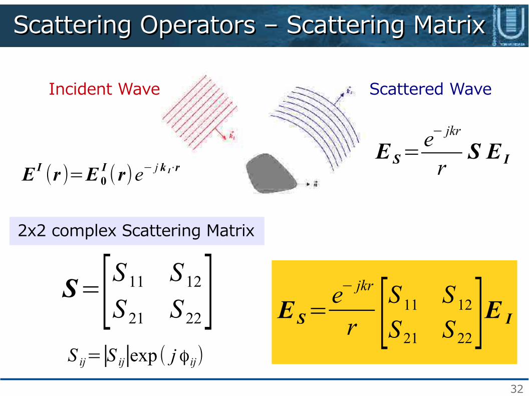
Scattering Operators – Scattering MatrixScattering Operators – Scattering Matrix
S qp=∣S qp∣exp ( j ϕqp)
σ=4π r2(∣E S∣)
2
(∣E I∣)2
σ qp=4π r2 (∣E S
q∣)2
(∣E Ip∣)2
σ0=⟨σ⟩
A0
σ qp=4π(∣S qp∣)2
Radar Cross Section Normalized Radar Cross Section
32
Scattering Operators – Scattering MatrixScattering Operators – Scattering Matrix
E S=e− jkr
r [S 11 S 12S 21 S 22]E I
E S=e− jkr
rS E I
S ij=∣S ij∣exp ( j ϕij)
Incident Wave Scattered Wave
S=[S 11 S 12S 21 S 22]
2x2 complex Scattering Matrix
E I (r )=E 0I (r)e− j k I⋅r

33
Scattering Operators – Scattering MatrixScattering Operators – Scattering Matrix
S=1
√4π [√σ11exp ( j ϕ11) √σ12exp ( j ϕ12)√σ21exp ( j ϕ21) √σ22exp ( j ϕ22)]
S=1
√4π [ √σ11 √σ12exp ( j (ϕ12−ϕ11))
√σ12exp ( j (ϕ12−ϕ11)) √σ22exp ( j (ϕ22−ϕ11))]
Scattering Matrix
Removing Absolute Phase (no info) + Considering Reciprocity Theorem

34
Scattering Operators – Mueller MatrixScattering Operators – Mueller MatrixRelation between Incident and Scattered Fields
Scattering Matrix - S
Mueller Matrix - M
Kennaugh Matrix - K
Jones formalism
Stokes formalism
Powers (Mueller using BSA)
S
M K

35
Polarization SynthesisPolarization SynthesisTechnique that permits the calculation of the response of the target for every possible combination of transmitting and receiving antennas.
σ qp=4π r2 (∣E q
r⋅E ps∣)
2
(∣E qr∣)2(∣E p
t∣)2=2π
J qrT K J p
t
(∣E qr∣)2(∣E p
t∣)2=2π jq
rT K j pt
For imaging radars, the individual measurements for each resolution element are statistically related, therefore several power measurements are added to reduce statistical variations.
σ pq0 =2π j q
rT ⟨K ⟩ j pt

36
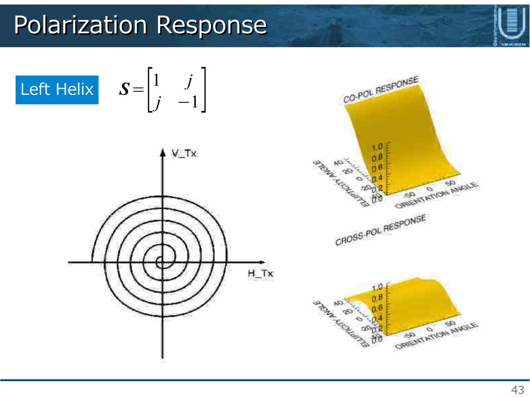
Polarization ResponsePolarization Response
Large conducting sphere S=[1 00 1]

37
Polarization ResponsePolarization Response
S=[−1 00 1]Dihedral Corner Reflector

38
Polarization ResponsePolarization Response
S=[1 00 1]Trihedral Corner Reflector

39
Polarization ResponsePolarization Response
S=[ cos(α)2 1
2sin (2α)
12sin(2α) sin (α)2 ]
α=0°
Oriented Dipole

40
Polarization ResponsePolarization Response
S=[ cos(α)2 1
2sin (2α)
12sin(2α) sin (α)2 ]
α=45°
Oriented Dipole

41
Polarization ResponsePolarization Response
S=[ cos(α)2 1
2sin (2α)
12sin(2α) sin(α)2 ]
α=90°
Oriented Dipole

42
Polarization ResponsePolarization Response
S=[ 1 − j− j 1 ]Right Helix
43
Polarization ResponsePolarization Response
S=[1 jj −1]Left Helix

44
Scattering Operators – Target VectorsScattering Operators – Target Vectors
S=[SHH SHVSVH SVV ]→ k=
12Tr {ψ S }
ψP={√2[1 00 1], √2[1 0
0 −1], √2[0 11 0]} ψL={2[1 0
0 0], 2√2[0 10 0], 2[0 0
0 1]}
Pauli Spin matrix basis set
Lexicograph matrix basis set
Construction of a vector describing the polarization state of the target
kP=1
√2[SHH+SVV S HH−SVV 2SHV ]
TkL=[S HH √2 S HV SVV ]
T
Physical properties of the target System measurables

45
Scattering Operators – Coherency MatrixScattering Operators – Coherency Matrix
kP=1
√2[SHH+SVV S HH−SVV 2SHV ]
T
T 3=[(∣S HH+SVV∣)
2(SHH+SVV )(S HH−SVV )
✳ (SHH+SVV )(2SHV )✳
(S HH−SVV )(SHH+SVV )✳
(∣S HH+SVV∣)2
(SHH−SVV )(2SHV )✳
(2SHV )(S HH+SVV )✳
(2SHV )(S HH−SVV )✳
(∣2 S HV∣)2 ]
T 3=kP⋅kP✳ T
Coherency matrix

46
Scattering Operators – Covariance MatrixScattering Operators – Covariance Matrix
kL=[S HH √2 S HV SVV ]T
C 3=kL⋅kL✳T
Covariance matrix
C 3=[(∣S HH∣)
2(S HH )(√2 SHV )
✳(SHH )(SVV )
✳
(√2 S HV )(S HH)✳ (∣2SHV∣)
2(√2 SHV )(SVV )
✳
(SVV )(S HH )✳ (SVV )(√2 S HV )
✳(∣SVV∣)
2 ]

47
Scattering Operators – Covariance MatrixScattering Operators – Covariance Matrix
C 3=12 [1 1 00 0 √21 −1 0 ]T 3[
1 0 11 0 −10 √2 0 ]
Relation between Coherency and Covariance matrices

48
Scattering Operators – Covariance MatrixScattering Operators – Covariance Matrix
Target Reflection Symmetry Assumption
(S HH)(S HV )✳=(SHV )(SVV )
✳=0
C 3=[(∣S HH∣)
2 0 (SHH )(SVV )✳
0 (∣2SHV∣)2 0
(SVV )(S HH )✳ 0 (∣SVV∣)
2 ]5 unknowns

49
Scattering Operators – Covariance MatrixScattering Operators – Covariance Matrix
Target Rotation Symmetry Assumption
C 3=[(∣SHH∣)
2 √2 (SHH )(S HV )✳ (∣SHH∣)
2−2 (∣S HV∣)
2
−√2(SHH )(SHV )✳ (∣2SHV∣)
2 √2(S HV )(S HH )✳
(∣SHH∣)2−2 (∣S HV∣)
2−√2 (S HV )(S HH )
✳ (∣SHH∣)2 ]
The Matrix remains unchanged under the transformation
T 3(θ)=R3(θ)T 3 R3(θ)−1
R3(θ)=[1 0 00 cos (2θ) sin (2θ)0 −sin (2θ) cos (2θ)] 3 unknowns

50
Scattering Operators – Covariance MatrixScattering Operators – Covariance Matrix
Target Azimuthal Symmetry Assumption
C 3=[(∣SHH∣)
2 0 (∣S HH∣)2−2(∣SHV∣)
2
0 (∣2SHV∣)2 0
(∣SHH∣)2−2 (∣S HV∣)
2 0 (∣S HH∣)2 ]
Combines both of the previous properties
2 unknowns

51
SECTION III
Polarimetric Features

52
Polarimetric FeaturesPolarimetric Features
Backscattering Coefficients
Polarimetric Ratios
Copol Phase Difference
Polarimetric Coherence
Eigenvalues Parameters
Target Vector Decomposition Components
Span

53
Features - SpanFeatures - Span
-30 dB >5 dB
SPAN=(∣SHH∣)2+(∣S HV∣)
2+(∣SVH∣)
2+(∣SVV∣)
2
OpticalGoogle Earth ©
RadarSat-2Fine Quad
Total Power

54
Features – Backscattering CoefficientsFeatures – Backscattering Coefficients
-30 dB >5 dB
σHH0
σHV0
σVV0

55
Features – Co-Pol & De-Pol RatiosFeatures – Co-Pol & De-Pol Ratios
-10 dB 8 dB -30 dB 0 dB
σVV0
σHH0
Co-Pol Ratio
σHV0
σHH0 +σVV
0
De-Pol Ratio

56
Features – Co-Pol Phase DifferenceFeatures – Co-Pol Phase Difference
π
π/2π/ 4
0−π/4
−π
−π/2
ϕ=Arg (SHH SVV✶)

57
Features – Polarimetric CoherenceFeatures – Polarimetric Coherence
0 1
ρAA−BB=⟨S AAS BB
✶⟩
√ ⟨∣S AA2∣⟩ ⟨∣S BB2∣⟩
∣ρHH−VV∣ ∣ρHH−HV∣
ππ2
0−π −π2
Arg (ρHH−HV )

58
Features – Target vector ComponentsFeatures – Target vector Components- Imaging Radars -
From Single “Pure” Target to Distributed Target
T=kP⋅k P✳ T
T=1N∑i=1
N
k i⋅k i✳ T

59
Features – Target vector ComponentsFeatures – Target vector Components
Target Decomposition Theorems aim to extract the mean or dominant scattering mechanisms or to separate different scattering contributions.
COHERENT DECOMPOSITIONSMODEL BASED
EIGENVALUES ANALYSIS
ENTROPY/ALPHA/ANISOTROPY
TARGET DICHOTOMY
Pauli, Krogager, Cameron, Touzi Freeman-Durden,Yamaguchi
Cloude
Cloude, Pottier
Huynen, Barnes, Holm

60
Features – Coherent DecompositonsFeatures – Coherent Decompositons
(∣SHH+SVV∣)2[dB ](∣SHH−SVV∣)
2[dB ] (2∣S HV∣)
2[dB ]
RED channel BLUE channel GREEN channel
Pauli

61
Features – Coherent DecompositonsFeatures – Coherent Decompositons
RGB Composite Image

62
Features – Model Based DecompositonsFeatures – Model Based DecompositonsReflection symmetry consideredFreeman-Durden
C 3=C 3S( f s)+C 3D( f d )+⟨C 3V( f v)⟩θ
Canopy scatter from a cloud of randomly oriented dipoles
Double bounce from a pair of orthogonal surfaces
Bragg scattering from a moderately rough surface
PTOT=PS ( f s)+PD( f d )+PV ( f v)
TARGET GENERATORS

63
Features – Model Based DecompositonsFeatures – Model Based Decompositons
PD [dB ] P S [dB ] PV [dB ]
RED channel BLUE channel GREEN channel

64
Features – Model Based DecompositonsFeatures – Model Based Decompositons
RGB Composite Image

65
Features – Eigenvalues DecompositonsFeatures – Eigenvalues Decompositons
T 3=U 3ΣU 3−1
Hermitian averaged 3x3 Coherency matrix in diagonal form
U 3=[u1 u2 u3 ]
Σ=[λ1 0 00 λ2 00 0 λ3
]λ1≥λ2≥λ3≥0
Eigenvectors of Coherency matrix
Eigenvalues of Coherency matrix
T 3=∑i=1
3
λ iu i⋅u i✳ T=T 01+T 02+T 03
Cloude

66
Features – Eigenvalues DecompositonsFeatures – Eigenvalues Decompositons
Single scattering mechanisms“weight” of scattering mechanism
T 01=λ1u1⋅u1✳ T=k 1⋅k1
✳T T 01=[T 1101 T 12
01 T 1301
T 2101 T 22
01 T 2301
T 3101 T 32
01 T 3301]
TARGET GENERATORSExtraction of the dominant
Scattering mechanism
T 3=∑i=1
3
λ iu i⋅u i✳ T=T 01+T 02+T 03

67
Features – Eigenvalues DecompositonsFeatures – Eigenvalues Decompositons
T 1101[dB ] T 22
01 [dB ] T 3301[dB ]
RED channel BLUE channel GREEN channel

68
Features – Eigenvalues DecompositonsFeatures – Eigenvalues Decompositons
RGB Composite Image

69
Features – H/alpha/A Features – H/alpha/A ENTROPY/ALPHA/ANISOTROPY
T 3=∑i=1
3
λ iu i⋅u i✳ T
Only one non zero = pure target = single scattering mechanismλ i
All three equal = random target = 3 orthogonal mechanismsλ i
U 3=[u1 u2 u3 ]
Scattering interpreted as a 3 symbol Bernoulli process occurring with pseudoprobabilities
P i=λ i
∑k=1
3
λk ∑ P i=1
with
PROBABILISTIC MODEL FOR SCATTERING

70
Features – H/alpha/A Features – H/alpha/A
U 3=[u1 u2 u3 ]
Parametrized as:
U 3=[cosα1 e
j ϕ1 cosα2 ej ϕ 2 cosα3 e
j ϕ3
sinα1 cosβ1ej(δ1+ϕ1) sinα2cosβ2e
j(δ2+ϕ2) sinα3 cosβ3 ej (δ3+ϕ3)
sinα1 cosβ1ej(γ1+ϕ 1) sinα2 cosβ2 e
j(γ2+ϕ2) sinα3 cosβ3 ej (γ3+ϕ3)]
The probabilistic approach allows the definition of mean scattering mechanism
u=ej ϕ[
cos αsin α cos βe j δ
sin α cos βe j γ] With mean parametersα ,β , δ , γ

71
Features – H/alpha/A Features – H/alpha/A
The only mean parameter following the roll-invariance property
α=∑kPkα k
MEAN ALPHA ANGLE
0⩽α⩽π
2
α≃0
α≃π
4
α≃π
2
Surface scattering
Scattering from acloud of particles
Double-bouncescattering

72
Features – H/alpha/A Features – H/alpha/A
ENTROPY
H=−∑k=1
3
Pk log3 Pk
H≃1
H≃0Pure target
Random target
Degree of mixing of various scattering mechanisms
0⩽H⩽1

73
Features – H/alpha/A Features – H/alpha/A
ANISOTROPY
A=λ 2−λ3λ 2+λ3
In High Entropy Areas, describes the behaviour of the scattering mechanisms apart from the dominant
A≃1
A≃01 high + 2 equal low
2 equal high + 1 low
0⩽A⩽1

74
SECTION IV
Applications

75
ApplicationsApplicationsLand Cover
Surface Parameter Estimation
Agriculture
Forestry
Urban
Ocean
Cryosphere
Target Detection

76
Land CoverLand Cover
Urban Expansion Monitoring
Wildlife Habitat Protection Resource Inventory and Management
Damage Delineation

77
Land CoverLand Cover
Detection of scattering mechanism
Target Decomposition Components & Wishart Classifier for Unsupervised Classification
Geometry recognition allows better classification accuracies
J.-S. Lee, M. Grunes, E. Pottier, and L. Ferro-Famil, “Unsupervised terrain classication preserving polarimetric scattering characteristics," 2004.
F. Xu and Y.-Q. Jin, “Deorientation theory of polarimetric scattering targets and application to terrain surface classication," 2005.
A. Lonnqvist, Y. Rauste, M. Molinier, and T. Hame, “Polarimetric SAR Data in Land Cover Mapping in Boreal Zone," 2010.
Z. Qi, A. G.-O. Yeh, X. Li, and Z. Lin, “A novel algorithm for land use and land cover classication using RADARSAT-2 polarimetric SAR data," 2012.
O. Antropov, Y. Rauste, A. Lonnqvist, and T. Hame, “Polsar mosaic normalization for improved land-cover mapping," 2012.
L. Loosvelt, J. Peters, H. Skriver, B. De Baets, and N. Verhoest, “Impact of reducing polarimetric sar input on the uncertainty of crop classifications based on the random forests algorithm," 2012.

78
Surface Parameter EstimationSurface Parameter Estimation
Important sources for hydrological or meteorological modeling, geology or agriculture monitoring.
Surface Roughness
Soil Moisture
Valuable techniques developed for dual-pol/quad-pol low frequency SAR.
Estimation is not possible using single polarization systems.One of the major issues is how roughness appears to be to radars.

79
Surface Parameter EstimationSurface Parameter Estimation
D. Schuler, J.-S. Lee, D. Kasilingam, and G. Nesti, “Surface roughness and slope measurements using polarimetric sar data," 2002.
I. Hajnsek, E. Pottier, and S. Cloude, “Inversion of surface parameters from polarimetric sar," 2003.
A. Iodice, A. Natale, and D. Riccio, “Retrieval of soil surface parameters via a polarimetric twoscale model," 2011.
N. Baghdadi, R. Cresson, E. Pottier, M. Aubert, M. Zribi, A. Jacome, and S. Benabdallah, “A potential use for the c-band polarimetric sar parameters to characterize the soil surface over bare agriculture fields," 2012.
Y. Kim and J. van Zyl, “A Time-Series Approach to Estimate Soil Moisture Using Polarimetric Radar Data," 2009.
I. Hajnsek, T. Jagdhuber, H. Schon, and K. Papathanassiou, “Potential of Estimating Soil Moisture Under Vegetation Cover by Means of PolSAR," 2009.
H. McNairn, C. Duguay, B. Brisco, and T. Pultz, “The effect of soil and crop residue characteristics on polarimetric radar response," 2002.
X-Bragg model
Two Scale model
Multitemporal Approach
Retrieval using Coherence

80
AgricultureAgriculture
Short-wavelength SAR, such as X- and C-bands, interacts mainly with the top part of canopy layers.
Pedestal height, HV or RR backscattering coefficients.
Characterization of type and amount of cover.
Differential extinction coefficient.
Biophysical parameters retrieval.
Multiple polarizations. Crops classification.
C-band Multipol, C-band Quadpol, X-band Dualpol.
Rice, sugarcane, wheat growth monitoring.
Vegetation Water Content retrieval.
Wetland characterization and flood monitoring.

81
AgricultureAgriculture
J. Lopez-Sanchez, J. Ballester-Berman, and J. Fortuny-Guasch, “Indoor wide-band polarimetric measurements on maize plants: a study of the dierential extinction coecient," 2006.S. Brown, S. Quegan, K. Morrison, J. Bennett, and G. Cookmartin, “High-resolution measurements of scattering in wheat canopies-implications for crop parameter retrieval," 2003.D. Hoekman and M. Vissers, “A new polarimetric classication approach evaluated for agricultural crops," 2003.K. Stankiewicz, “The effciency of crop recognition on ENVISAT ASAR images in two growing seasons," 2006.H. Skriver, F. Mattia, G. Satalino, A. Balenzano, V. Pauwels, N. Verhoest, and M. Davidson, “Crop classication using short-revisit multitemporal sar data," 2011.H. Skriver, “Crop Classication by Multitemporal C- and L-Band Single- and Dual-Polarization and Fully Polarimetric SAR," 2012.H. McNairn, J. Shang, X. Jiao, and C. Champagne, “The contribution of alos palsar multipolarization and polarimetric data to crop classication," 2009.J. Chen, H. Lin, and Z. Pei, ”Application of ENVISAT ASAR Data in Mapping Rice Crop Growth in Southern China," 2007.F. Wu, C. Wang, H. Zhang, B. Zhang, and Y. Tang, “Rice Crop Monitoring in South China With RADARSAT-2 Quad-Polarization SAR Data," 2011.S. Yang, X. Zhao, B. Li, and G. Hua, “Interpreting RADARSAT-2 Quad-Polarization SAR Signatures From Rice Paddy Based on Experiments," 2012.J. Lopez-Sanchez, J. Ballester-Berman, and I. Hajnsek, “First results of rice monitoring practices in spain by means of time series of terrasar-x dual-pol images," 2011.J. Lopez-Sanchez, S. Cloude, and J. Ballester-Berman,”Rice Phenology Monitoring by Means of SAR Polarimetry at X-Band," 2012.W. Koppe, M. L. Gnyp, and C. H “Rice monitoring with multi-temporal and dual-polarimetric TerraSAR-X data," 2012.H. Lin, J. Chen, Z. Pei, S. Zhang, and X. Hu, “Monitoring Sugarcane Growth Using ENVISAT ASAR Data," 2009.G. Satalino, F. Mattia, T. Le Toan, and M. Rinaldi, ”Wheat Crop Mapping by Using ASAR AP Data," 2009.C. Notarnicola and F. Posa, “Inferring Vegetation Water Content From C- and L-Band SAR Images," 2007.B. Marti-Cardona, C. Lopez-Martinez, J. Dolz-Ripolles, and E. Blade-Castellet, ”ASAR polarimetric, multi-incidence angle and multitemporal characterization of Donana wetlands for floode extent monitoring," 2010.R. Touzi, A. Deschamps, and G. Rother, ”Phase of target scattering for wetland characterization using polarimetric c-band sar," 2009.

82
ForestryForestryNeed to develop a biomass cartography of the whole planet. Carbon cycle monitoring.
Frequency dependance of biomass.
P- L- C- band Quadpol (AIRSAR - NASA)
Forest structure
Tree height
Stand age retrieval.
Forestry is an applicative field where lower frequency bands demonstrated to be useful, as the penetration of longer wavelenghts is proved to be essential for biomass retrieval.
Coherence.
Backscattering Coefficients.
Entropy/Alpha/Anisotropy.
Specific field of research and applications: POLinSAR – Polarimetry & Interferometry

83
ForestryForestry
J. Kellndorfer, M. Dobson, J. Vona, and M. Clutter, “Toward precision forestry: plot-level parameter retrieval for slash pine plantations with JPL AIRSAR," 2003.
M.Watanabe, M. Shimada, A. Rosenqvist, T. Tadono, M. Matsuoka, S. Romshoo, K. Ohta, R. Furuta, K. Nakamura, and T. Moriyama, “Forest Structure Dependency of the Relation Between L-Band and Biophysical Parameters," 2006.
H. Wang and K. Ouchi, “Accuracy of the K -Distribution Regression Model for Forest Biomass Estimation by High-Resolution Polarimetric SAR: Comparison of Model Estimation and Field Data," 2008.
D. Hoekman and M. Quinones, “Biophysical forest type characterization in the Colombian Amazonn by airborne polarimetric SAR," 2002.
F. Garestier, P. Dubois-Fernandez, D. Guyon, and T. Le Toan, “Forest Biophysical Parameter Estimation Using L- and P-Band Polarimetric SAR Data," 2009.
S. McNeill and D. Pairman, ”Stand age retrieval in production forest stands in New Zealand using C- and L-band polarimetric Radar," 2005.
Y. Maghsoudi, M. Collins, and D. G. Leckie, “Polarimetric classication of Boreal forest using nonparametric feature selection and multiple classiers," 2012.
S. Maity, C. Patnaik, J. Parihar, S. Panigrahy, and K. Reddy, “Study of physical phenomena of vegetation using polarimetric scattering indices and entropy," 2011.

84
UrbanUrbanCapability of recognizing and separating different scattering mechanisms.
High resolution images
Entropy/Alpha/Anisotropy approach.Polarizaton orientation angle.
Classification of urban/suburban areas.
Circular Pol Correlation Coefficient. Characterization of man-made structures.
Monitoring of damaged areas after earthquakes.
C- and L- band full polarimetric data.
Characterization of different scattering mechanisms. Urban density information extraction.
+
San Francisco X-band QuadPol Stripmap (5m)

85
UrbanUrbanSPAN Circular Correlation
Coefficient

86
UrbanUrban
T. M. Pellizzeri, “Classication of polarimetric SAR images of suburban areas using joint annealed segmentation and H/A/alpha polarimetric decomposition," 2003.
T. Ainsworth, D. Schuler, and J.-S. Lee, “Polarimetric SAR characterization of man-made structures in urban areas using normalized circular-pol correlation coefficients," 2008.
K. Iribe and M. Sato, “Analysis of polarization orientation angle shifts by articial structures," 2007.
M. Watanabe, T. Motohka, Y. Miyagi, C. Yonezawa, and M. Shimada, “Analysis of Urban Areas Affected by the 2011 O the Pacific Coast of Tohoku Earthquake and Tsunami With L-Band SAR Full-Polarimetric Mode," 2012.
X. Li, H. Guo, L. Zhang, X. Chen, and L. Liang, “A New Approach to Collapsed Building Extraction Using RADARSAT-2 Polarimetric SAR Imagery," 2012.
R. Schneider, K. Papathanassiou, I. Hajnsek, and A. Moreira, “Polarimetric and interferometric characterization of coherent scatterers in urban areas," 2006.
M. Fujita and Y. Miho, “Analysis of a microwave backscattering mechanism from a small urban area imaged with sir-c," 2006.
87
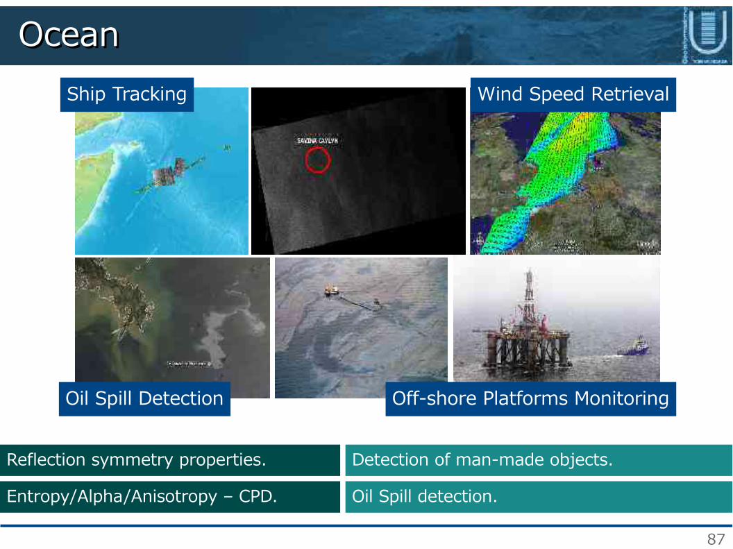
OceanOceanShip Tracking
Oil Spill Detection Off-shore Platforms Monitoring
Wind Speed Retrieval
Reflection symmetry properties. Detection of man-made objects.
Entropy/Alpha/Anisotropy – CPD. Oil Spill detection.

88
OceanOcean
M. Migliaccio, A. Gambardella, and M. Tranfaglia, “SAR Polarimetry to Observe Oil Spills," 2007.
M. Migliaccio, A. Gambardella, F. Nunziata, M. Shimada, and O. Isoguchi, “The PALSAR Polarimetric Mode for Sea Oil Slick Observation," 2009.
M. Migliaccio, F. Nunziata, A. Montuori, X. Li, and W. Pichel, “A Multifrequency Polarimetric SAR Processing Chain to Observe Oil Fields in the Gulf of Mexico," 2011.
D. Velotto, M. Migliaccio, F. Nunziata, and S. Lehner, ”Dual-Polarized TerraSAR-X Data for Oil-Spill Observation," 2011.
R. Touzi, R. Raney, and F. Charbonneau, “On the use of permanent symmetric scatterers for ship characterization," 2004.
X. Li and J. Chong, “Processing of Envisat Alternating Polarization Data for Vessel Detection," 2008.
J. Chen, Y. Chen, and J. Yang, “Ship detection using polarization cross-entropy," 2009.
B. Zhang, W. Perrie, P. W. Vachon, X. Li, W. G. Pichel, J. Guo, and Y. He, “Ocean vector winds retrieval from c-band fully polarimetric sar measurements," 2012.

89
CryosphereCryosphere
Snow Characterization Glaciers Monitoring Ship routing
VV-HH backscattering L- X-band. Ice thickness retrieval.
Cross polarization channel. Depol. Discrimination between FYI/ MYI
C-band Full pol. Classification of glaciers.

90
CryosphereCryosphere
K. Nakamura, H.Wakabayashi, K. Naoki, F. Nishio, T. Moriyama, and S. Uratsuka, “Observation of sea-ice thickness in the sea of Okhotsk by using dual-frequency and fully polarimetric airborne SAR (pi-SAR) data," 2005.
K. Partington, J. Flach, D. Barber, D. Isleifson, P. Meadows, and P. Verlaan, “Dual-Polarization C-Band Radar Observations of Sea Ice in the Amundsen Gulf," 2010.
J.-W. Kim, D. jin Kim, and B. J. Hwang, “Characterization of arctic sea ice thickness using high resolution spaceborne polarimetric sar data," 2012.
L. Huang, Z. Li, B.-S. Tian, Q. Chen, J.-L. Liu, and R. Zhang, “Classication and snow line detection for glacial areas using the polarimetric SAR image," 2011.
J. Sharma, I. Hajnsek, K. Papathanassiou, and A. Moreira, “Polarimetric decomposition over glacier ice using long-wavelength airborne polsar," 2011.
M. Trudel, R. Magagi, and H. Granberg, “Application of Target Decomposition Theorems Over Snow-Covered Forested Areas," 2009.

91
Target DetectionTarget Detection
Target Ship Moving Object
Change inside the sceneUse of polarimetric properties or configurations for detection.
Reflection Symmetry. Man-made targets detection.
Phase difference between crosspol. Ambiguities detection.
Sensitivity of polarimetric coherence. Recognition similar features in different images.
Land cover classification.
Change detection.Polarization state conformation.

92
Target DetectionTarget Detection
N. Wang, G. Shi, L. Liu, L. Zhao, and G. Kuang, “Polarimetric sar target detection using the reflection symmetry," 2012.
C. Liu and C. Gierull, “A new application for polsar imagery in the field of moving target indication/ship detection," 2007.
A. Marino, S. Cloude, and I. Woodhouse, “A polarimetric target detector using the Huynen fork," 2010.
A. Marino, S. Cloude, and I. Woodhouse, “Detecting Depolarized Targets Using a New Geometrical Perturbation Filter," 2012.
A. Marino, S. R. Cloude, and J. M. Lopez-Sanchez, “A New Polarimetric Change Detector in Radar Imagery," 2012.
M. Qong, “Polarization state conformation and its application to change detection in polarimetric sar data," 2004.

93
Application MaturityApplication Maturity
DOMAIN APPLICATION/PRODUCT MATURITY NOTE
FORESTRY
ABOVE GROUND BIOMASS MEDIUM POLINSAR
STAND HEIGHT HIGH POLINSAR
VERTICAL STRUCTURE MEDIUM POLINSAR
THEMATIC MAPS HIGH
CHANGE DETECTION HIGH
AGRICULTURE
CROP TYPE MAPPING MEDIUM
SOIL MOISTURE HIGH
PHENOLOGY DETERMINATION MEDIUM
FLOODING MAPPING MEDIUM
CRYOSPHERE
SNOW VOLUME MEDIUM
LAND ICE EXTINCTION LOW
SEA ICE SURFACE CHARACTERIZATION LOW
URBANMAPPING/CLASSIFICATION MEDIUM
SUBSIDENCE MEDIUM
OCEANOIL SLICK DETECTION MEDIUM
METALLIC TARGETS MEDIUM
Results of ESA POLinSAR2013 – February 2013

94
SECTION V
Software

95
ESA PolSAR ProESA PolSAR ProLicence Free
Type Standalone application
Sensors Every polarimetric airborne/spaceborne sensor
Analysis Almost every polarimetric technique is implemented
Website http://earth.eo.esa.int/polsarpro/

96
ASF MapReadyASF MapReadyLicence Free
Type Standalone application
Sensors ALOS-Palsar Radarsat-2 TerraSAR-X CEOS-1 format
Analysis Pauli Compositon Sinclair Compositon
Cloude-Pottier Classification (8 and 16 classes)
Sinclair Compositon
Entropy/Alpha/Anisotropy Wishart Classifier
Freman/Durden
Faraday Rotarion Compensation
Website http://www.asf.alaska.edu/downloads/software_tools

97
Exelis SARScapeExelis SARScapeLicence Commercial
Type ENVI module
Sensors
Analysis Polarimetric Calibration
Polarization Signature
Entropy/Alpha/Anisotropy Decomposition and Classification
Pauli Composition
Polarization Synthesis
Most of commercial spaceborne sensors supported
Website http://www.exelisvis.com/ProductsServices/ENVI/SARscape.aspx

98
Radar ToolsRadar ToolsLicence Free
Type IDL Library
Sensors
Analysis
Most of commercial spaceborne sensors supported
Website http://radartools.berlios.de/
Point Target Analysis
Speckle Filtering
Entropy/Alpha/Anisotropy Decomposition and Classification
Decomposition Analysis
Edge Detectors Polarimetric Descriptors
Basis Transform Subaperture Analysis

99
Racurs Photomod RadarRacurs Photomod RadarLicence Commercial
Type Photomod Module
Sensors
Analysis Polarimetric Descriptors
Sinclair Composition
Entropy/Alpha/Anisotropy Decomposition and Classification
Pauli Composition
Classical Decompositions
Website http://www.racurs.ru/?page=86
ALOS-Palsar Radarsat-2 TSX CEOS-1 format CSK

100
PCI GeomaticaPCI GeomaticaLicence Commercial
Type PCI Module
Sensors
Website
Scattering, Covariance, Coherency, Kennaugh Matrices
Correlation Coeff.
Entropy/Alpha/Anisotropy Decomposition and Classification
Pauli Composition
Pedestal Height
Most of commercial spaceborne sensors supported
Total Power and Ratios
Phase Differences
Classical Decompositions (Freeman, VanZyl, Huynen, ...)
Speckle Filters
http://www.pcigeomatics.com/products/geomatica-2013

101
SECTION VI
Conclusions

102
Conclusions – Scattering and PolarizationConclusions – Scattering and PolarizationEM Scattering – Wavelength dependance
Surface Roughness
Volume Penetration
Smooth Rough Very RoughIncident
Coherent
Incoherent
L band C band X band

103
Conclusions – Scattering and PolarizationConclusions – Scattering and Polarization
L
C
X
San Francisco Airport Multifrequency effect of Model-Based Freeman Decomposition

104
L
C
X
Treasure IslandYerba Buena Island
Multifrequency effect of Model-Based Freeman Decomposition
Conclusions – Scattering and PolarizationConclusions – Scattering and Polarization

105
Conclusions – Scattering and PolarizationConclusions – Scattering and Polarization
L
C
X
Golden Gate Bridge Multifrequency effect of Model-Based Freeman Decomposition

106
Conclusions – ModelsConclusions – Models
k σ z
k l c
EM Surface Scattering ModelsSmall PerturbationModel
Integral EquationMethod
Geometric Optics Approximation
σ z - Rms surface height variationsl c - Surface autocorrelation length
k - Wavenumber

107
Full vs Dual PolFull vs Dual Pol
Full Polarimetry Dual Polarimetry
Target ScatteringCharacterization
Range Ambiguities Doubled Data Tx/Rx
Doubled Azimuth Resolution
Double Swath Width
Complete Polarimetric Info
Halved Swath Width
HH-VV Phase HV/VH Information
Incomplete Polarimetric Info
No HH-VV Phase and HV/VH
- Geometry - Material
- Depolarization
- Cross-Polarization
Partial Target ScatteringCharacterization
- Material

108
Conclusions – Other NSAConclusions – Other NSA
Sentinel-1A/B
Radarsat Constellation Mission
Alos-2
TerraSAR-L / TanDEM-L
SAOCOM
C-band Dual-Pol
C-band Dual/Compact/Quad-Pol
L-band Dual/Compact/Quad-Pol
L-band TanDEM
L-band Dual/Compact/Quad-Pol
“We have arrived at the door-steps of the golden age of polarimetric radar imaging.”
- Lee, Pottier - Polarimetric Radar Imaging, CRC 2009