space radiation cancer risk projections and … space radiation cancer risk projections and...

NASA/TP-2013-217375

Space Radiation Cancer Risk Projections and

Uncertainties – 2012

Francis A. Cucinotta

NASA Lyndon B. Johnson Space Center

Houston, Texas

Myung-Hee Y. Kim and Lori J. Chappell

U.S.R.A., Division of Space Life Sciences

Houston, Texas

January 2013

THE NASA STI PROGRAM OFFICE . . . IN PROFILE

Since its founding, NASA has been dedicated to the

advancement of aeronautics and space science. The

NASA Scientific and Technical Information (STI)

Program Office plays a key part in helping NASA

maintain this important role.

The NASA STI Program Office is operated by

Langley Research Center, the lead center for NASA’s

scientific and technical information. The NASA STI

Program Office provides access to the NASA STI

Database, the largest collection of aeronautical and

space science STI in the world. The Program Office

is also NASA’s institutional mechanism for dissemi-

nating the results of its research and development

activities. These results are published by NASA in

the NASA STI Report Series, which includes the

following report types:

• TECHNICAL PUBLICATION. Reports of

completed research or a major significant phase

of research that present the results of NASA pro-

grams and include extensive data or theoretical

analysis. Includes compilations of significant

scientific and technical data and information

deemed to be of continuing reference value.

NASA’s counterpart of peer-reviewed formal

professional papers but has less stringent limita-

tions on manuscript length and extent of graphic

presentations.

• TECHNICAL MEMORANDUM. Scientific

and technical findings that are preliminary or

of specialized interest, e.g., quick release reports,

working papers, and bibliographies that contain

minimal annotation. Does not contain extensive

analysis.

• CONTRACTOR REPORT. Scientific and

technical findings by NASA-sponsored

contractors and grantees.

• CONFERENCE PUBLICATION. Collected

papers from scientific and technical conferences,

symposia, seminars, or other meetings sponsored

or cosponsored by NASA.

• SPECIAL PUBLICATION. Scientific, technical,

or historical information from NASA programs,

projects, and mission, often concerned with

subjects having substantial public interest.

• TECHNICAL TRANSLATION. English-

language translations of foreign scientific and

technical material pertinent to NASA’s mission.

Specialized services that complement the STI

Program Office’s diverse offerings include creating

custom thesauri, building customized databases, or-

ganizing and publishing research results . . . even

providing videos.

For more information about the NASA STI Program

Office, see the following:

• Access the NASA STI Program Home Page at

http://www.sti.nasa.gov

• E-mail your question via the Internet to

[email protected]

• Fax your question to the NASA Access Help

Desk at (301) 621-0134

• Telephone the NASA Access Help Desk at (301)

621-0390

• Write to:

NASA Access Help Desk

NASA Center for AeroSpace Information

7121 Standard

Hanover, MD 21076-1320

NASA/TP-2013-217375

Space Radiation Cancer Risk Projections and

Uncertainties – 2012

Francis A. Cucinotta

NASA Lyndon B. Johnson Space Center

Houston, Texas

Myung-Hee Y. Kim and Lori J. Chappell

U.S.R.A., Division of Space Life Sciences

Houston, Texas

January 2013

Available from:

NASA Center for AeroSpace Information National Technical Information Service

7121 Standard Drive 5285 Port Royal Road

Hanover, MD 21076-1320 Springfield, VA 22161

This report is also available in electronic form at http://ston.jsc.nasa.gov/collections/TRS

i

Contents

Acronyms and Nomenclature............................................................................................................. iii

Preface ............................................................................................................................................... vi

Executive Summary ........................................................................................................................... xiv

1. Introduction. .............................................................................................................................. 1

1.1 Uncertainty Assessments and Classification .................................................................... 3

1.2 Basic Concepts ................................................................................................................. 6

2. Space Radiation Environments and Transport Models ......................................................... 9

2.1 Galactic Cosmic Ray Models ........................................................................................... 10

2.1.1 Model of galactic cosmic rays charge and energy spectra .................................... 10

2.1.2 Isotopic composition of galactic cosmic rays ....................................................... 11

2.1.3 Solar modulation of the galactic cosmic rays ....................................................... 14

2.2 Solar Particle Events ........................................................................................................ 18

2.2.1 Hazard function for solar particle event occurrence ............................................. 20

2.2.2 Representation of solar particle event energy distribution ................................... 22

2.3 Physics Model Description of Organ Exposures ............................................................. 24

2.3.1 Comparisons of ground-based measurements to transport codes ......................... 26

2.3.2 Comparisons of transport codes ........................................................................... 28

2.3.3 Space flight measurement comparisons to transport codes .................................. 30

2.3.4 Predictions for exploration missions .................................................................... 34

2.4 Dose Contributions from Pions and Pion Decays ............................................................ 38

2.5 Probability Distribution Function for Space Physics Uncertainties ................................. 40

2.6 Summary of Research Needs in Space Physics ............................................................... 41

3. Cancer Risk Projections for Low-linear Energy Transfer Radiation .................................. 42

3.1 Cancer Mortality and Incident Rates ............................................................................... 43

3.2 Adjustment for Low Dose-rates ....................................................................................... 45

3.3 Comparisons of Tissue-specific Risk Models .................................................................. 46

3.4 Age at Exposure Dependence of Cancer .......................................................................... 46

3.5 Other Methods for Incidence to Mortality Conversion .................................................... 50

3.6 Reference Population Data for Astronauts ....................................................................... 55

3.6.1 Healthy Worker Effects and Risk Estimates ........................................................ 62

3.6.2 Baseline Cancer Rates and Life-table Data .......................................................... 63

3.7 Summary of Research Needs for Type I Uncertainties .................................................... 67

4. Uncertainties in Low-linear-energy-transfer Risk Model Factors ........................................ 68

4.1 Life-span Study Dosimetry Errors ................................................................................... 69

4.2 Statistical Errors ............................................................................................................... 69

4.3 Errors from Reporting Bias .............................................................................................. 70

4.4 Dose-Rate Reduction Factor Uncertainties ...................................................................... 70

4.4.1 Re-analysis of DDREF using BEIR VII Approach .............................................. 72

4.4.2 Combining the distributions using Bayesian methods .......................................... 74

4.5 Transfer Models Uncertainties ......................................................................................... 77

4.6 Summary of Past Uncertainty Analysis for Low-linear Energy Transfer Radiation ....... 80

4.7 Summary of Research Needs on Type II Uncertainties and Human DDREF Data ......... 80

ii

5. Cancer Risks and Radiation Quality ....................................................................................... 81

5.1 Radiobiology Data for Relative Biological Effectiveness ............................................... 82

5.1.1 Relative biological effectiveness from human epidemiology studies................... 82

5.1.2 Animal carcinogenesis studies with heavy ions ................................................... 83

5.1.3 Cellular studies on chromosomal aberrations and mutation ................................. 87

5.2 Qualitative Differences of HZE Particles and Low LET Radiation ................................. 89

5.3 Biophysical Considerations.............................................................................................. 91

5.4 Biophysical Models of Relative Biological Effectiveness ............................................... 97

5.4.1 Relative biological effectiveness in the non-targeted effects model .................... 100

5.4.2 Saturation mechanisms in biological responses ................................................... 104

5.5 Risk Cross Sections and Coefficients .................................................................... …….. 104

5.6 NASA Radiation Quality Factors .................................................................................... 106

5.6.1 Parameter estimation for NASA Quality Factors and uncertainties ..................... 106

5.7 Recommendations for Research Needs on Radiation Quality ......................................... 114

6. Revised NASA Model for Cancer Risks and Uncertainties ................................................... 115

6.1 Track-structure-based Risk Model ................................................................................... 118

6.2 Updates to Radiation Transport Codes ............................................................................ 119

6.3 NASA Effective Dose and Tissue Weights ..................................................................... 122

6.4 Overall Uncertainty Assessment ...................................................................................... 126

6.4.1 Uncertainties due to Non-targeted effects ............................................................ 130

6.5 Considerations for Implementation of New Methods ...................................................... 131

7. Conclusions ................................................................................................................................ 133

8. References .................................................................................................................................. 138

Appendix A ................................................................................................................................. 156

Appendix B.................................................................................................................................. 160

iii

Acronyms and Nomenclature

ACE Advanced Composition Explorer

AGS alternating gradient synchrotron

AIC Akaiki information criteria

ALARA as low as reasonably achievable

AML acute myeloid leukemia

AU astronomical unit

BEIR (NAS) Committee on the Biological Effects of Ionizing Radiation

BFO blood-forming organ

BIC Bayesian information criteria

BMI body mass index

BNL Brookhaven National Laboratory

CA chromosomal aberrations

CAD computer-aided design

CAF computerized anatomical female

CAM computerized anatomical man

CAMERA computerized anatomical man model

CBA carcinoma-bearing animal

CDC Centers for Disease Control and Prevention

CDF Cumulative Distribution Function

CHD coronary heart disease

CI confidence intervals

CL confidence level

CME coronal mass ejection

CNS central nervous system

D dose

DDREF dose and dose-rate reduction effectiveness factor

DLOC dosimetry location

DNA deoxyribonucleic acid

DREF dose-rate effectiveness factor

DSB double-strand break

E kinetic energy

EAR excess additive risk

EB Empirical Bayes

ELR excess lifetime risk

EPA Environmental Protection Agency

ERR excess relative risk

ET extra-thoracic

F fluence (number of ions per unit area ions/cm2)

GCR galactic cosmic rays

GERMCode GCR Event-based Risk Model

GM geometric mean

GLE ground-level enhancement

GOES Geostationary Operational Environmental Satellite

GSD geometric standard deviation

Gy Gray

HZE high-energy and charge

IARC International Agency for Cancer Research

ICRP International Commission on Radiological Protection

IMP Interplanetary Monitoring Platform

iv

ISS International Space Station

kbp kilobase pairs

LAR lifetime attributable risk

LEO low-Earth orbit

LET linear energy transfer

LIS local interplanetary spectrum

LQ linear-quadratic

LSS Life-span Study (of the Japanese atomic-bomb survivors)

LTV lunar transfer vehicle

MARIE Martian Radiation Environment Experiment

MFISH multicolor fluorescence in-situ hybridization

MLE maximum likelihood estimate

MOLA Mars orbiter laser altimeter

NAS National Academy of Sciences

NCI National Cancer Institute

NCRP National Council of Radiation Protection and Measurements

NEO near-Earth object

NGDC National Geophysical Data Center

NHEJ non-homologous end-joining (repair)

NIH National Institutes of Health

NOAA National Oceanographic and Atmospheric Agency

NRC National Research Council

NS never-smokers

NS-NW never-smokers of normal-weight

NW normal weight

NSCLC non-small cell lung carcinoma

NSRL NASA Space Radiation Laboratory

NTE non-targeted effects

PDF probability distribution function

PEL permissible exposure limit

PRA probabilistic risk assessment

Q quality factor

QF quality factor

Q(L) quality factor as a function of LET

QMSFRG quantum multiple scattering fragmentation model

R0 low-LET risk coefficient per unit dose

RBE relative biological effectiveness

RBEmax maximum relative biological effectiveness that assumes linear responses at low doses or

dose-rates

REIC risk of exposure-induced cancer

REID risk of exposure-induced death

RERF Radiation Effects Research Foundation

RMAT Range-energy in Materials

RMS root mean square

RR relative risks

SCLC small cell lung carcinoma

SD standard deviation

SEER surveillance, epidemiology, and end results

SMR Standard Mortality Ratio

SPE solar particle event

SRP Space Radiation Program

v

SSA Social Security Administration

SSB single-strand break

TE targeted effects

TEPC tissue-equivalent proportional counter

TLD thermoluminescent dosimeter

UNSCEAR United Nations Special Committee on the Effects of Atomic Radiation

Z charge number

Z* effective charge number

coefficient of linear dose response term, Gy-1

coefficient of quadratic dose-response term, Gy-2

j(x,E) number of particles of type j with energy, E at depth, x in shielding, 1/(MeV/u cm2)

I gender- and age-specific cancer incidence rate, cancers/y

M gender- and age-specific cancer mortality rate, cancer deaths/y

parameter in action cross section to determine most biologically effects Z*2/

2

action cross section or probability of effect per unit fluence, m2

track structure derived risk cross section, m2

vi

Preface In 2010, NASA completed the development of a revised methodology for evaluating space radiation cancer risks for application to exploration mission trade studies and for evaluating crew risks for missions on the International Space Station (ISS). The model was denoted as NASA Space Cancer Risk Model-2010 (NSCR-2010).215 The revision was intended to update the earlier methodologies for projecting radiation cancer risks originating in NCRP Report 132 (2000) and our previous results for estimating uncertainties in space radiation risk estimates.12,14 The basis for the revision includes more recent human radiation epidemiology data and analysis, research results from the NASA Space Radiation Laboratory (opened for research in October 2003), and improved theoretical considerations.215 In 2011, the National Research Council (NRC) Space Science Board of the National Academy of Sciences began a review of the NASA Model 2010 by a panel of experts in the areas of space physics, radiobiology, epidemiology, and risk assessment. The review was published in March 2012.216 The purpose of the present report is to document NASA’s responses to the NRC recommendations, which include several updates of the NSCR-2010 model and discussion of points of clarification. In this Preface, we summarize the responses and point to sections of the revised report where changes are detailed. The revised model is denoted as NSCR-2012. NASA used the recommendations of the National Council of Radiation Protection and Measurements (NCRP) as the basis for the radiation protection programs including risk assessment models since 1989, as described in three NCRP reports published in 1989, 2000, and 2003. The NRC report216 places a large focus on the results from the National Academy of Sciences (NAS) BEIR VII Report16 and, to a lesser extent, changes NASA recommended relative to the NCRP models. The BEIR VII report introduced several new features to projection models that were adapted in the NSCR-2010 model. However, BEIR VII had specifically assumed radiation cancer rates are independent of age at exposure above age 30-y for most tissues.16 Since the age of exposure dependence of radiation cancer risks is a critical part of the NCRP recommendations used at NASA, the NASA model used the analysis of cancer rates from the United Nations Special Committee on the Effects of Atomic Radiation (UNSCEAR),17 which included age at exposure effects in fitting the same epidemiology data considered by BEIR VII. A comparison of the BEIR VII to the UNSCEAR models was made in our previous reports.215,221 The NSCR-2012 model uses the results from the UNSCEAR models for cancer incidence projections for most tissues, specifically because age at exposure dependencies are included in the UNSCEAR model. Many of the new methodologies suggested in the BEIR VII report were adapted in the NSCR-2010 and are part of the NSCR-2012 model. Chapter 2: Space Radiation Environments and Transport Models: From the 2012 NRC Report, “The Committee considers that the radiation environment and shielding transport models used in the NASA‟s proposed model are a major step forward compared to previous models used. This is especially the case for the statistical solar particle event model. The current models have been developed by making extensive use of the available data and rigorous mathematical analysis The uncertainties conservatively allocated to the space physics parameters are deemed to be adequate at this time, considering that the space physics uncertainties are only a minor contributor to the overall cancer risk assessment. Although further research in this area could reduce the uncertainty, the law of diminishing returns may prevail.”

vii

The 2012 NRC Report went on to make recommendations related to improving the understanding of the radial dependence of solar particle event (SPE) intensity and solar-cycle dependence of SPE frequency and extreme events. NASA is supporting a new effort with the Mars Science Laboratory Radiation Assessment Detector on the surface of Mars,217 and can continue to evaluate data from the Mars Radiation Environment Experiment (MARIE) instrument on Odyssey, and the Ulysses and Voyager spectrometers, which provide data on radial gradients. The NASA Science Mission Directorate has supported modeling efforts related to the propagation of solar particles,218 and these models could be coupled to the NASA Cancer Risk Model in the future. The statistical model of SPEs we have developed60,219 will continue to be updated, as suggested by the 2012 NRC Report.216 Since the development of the NASA 2010 model, new information related to the galactic cosmic rays (GCR) environment and the dose contributions from pion production due to GCR interactions with shielding and tissue, and electromagnetic decays that result from pion decays have become available. Analysis of the most recent solar minimum in 2009 was completed. The current report extends Chapter 2 to summarize this new information. Most importantly, the revised Badhwar-O’Neill GCR model, denoted as BO2011, is used in this report along with the resulting computer codes, thereby replacing the older model denoted as BO96 or other versions. An empirical correction for the dose from pions and their decays into gamma-rays, muons, and electrons is included in the NSCR-2012 model. These combined changes lead to a modest risk or dose equivalent reduction at solar minimum of about 5%. At other periods of the solar cycle, higher or lower values of up to 10% for BO11 compared to BO96 are found. Chapter 3: Cancer Risk Projections for Low-linear Energy Transfer Radiation 3.1 Incidence-Mortality Conversion Approach: In the NASA Model 2010, cancer mortality projections were made using the ―incidence-mortality‖ approach used by BEIR VII. The 2012 NRC Report noted, “A major reason for the use of the LSS cancer incidence data is that these are likely to be more accurate than are the mortality data, which suffer from misclassification of causes on death certificates”. The 2012 NRC Report went on to recommend: “Before NASA implements its proposed major change to the “incidence-mortality” approach, the committee recommends that NASA conduct more research into the specific patterns of the underlying epidemiological biases that drive these changes…the committee recommends that NASA consider alternative methods for improved estimation of mortality probabilities for each cancer site. For example, as presented in its 2011 report, „EPA Radiogenic Cancer Risk Models and Projections for the U.S. Population‟, the Environmental Protection Agency” has developed an alternative approach for breast cancer mortality estimation, and this could serve as a suitable approach to be applied by NASA”. NASA agrees with this recommendation. In response to this recommendation, we performed new analysis of incidence-mortality conversion models in Chapter 3 of this report. In considering these new analyses, we note that the Environmental Protection Agency (EPA) model,220 which was published after the NSCR 2010 model was submitted for review, has several strengths and weaknesses. One strength is that the EPA noted a time lag between cancer incidence and mortality data reported by the National Cancer Institute (NCI) surveillance, epidemiology, and end results (SEER) program due to either calendar year changes in cancer incidence rates, or changes in cancer cure rates, which is a potential confounder to mortality risk predictions. This confounder was shown in the EPA report to be important for breast cancer and would potentially impact other cancers in which the time between disease discovery and possible cancer death is long. The EPA used 5-year cancer survival probability data to convert radiation cancer incidence probabilities into mortality estimates. A weaknesses of the EPA model is their use of

viii

lifetime attributable risk (LAR), and not risk of exposure-induced death (REID) as a measure of risk. LAR is inaccurate for higher radiation exposures and in uncertainty analyses where large risk values occurs in Monte-Carlo sampling because LAR does not accurately account for competing risks. Using a similar approach for REID calculations complicates the application of 5-year or 10-year survival probabilities due to the nonlinear coupling of all cancer deaths in the analysis, while in the LAR the coupling is a simple addition of terms. A second problem is that the EPA used a constant hazard rate model based on patient survival data. We checked this assumption for lung and colorectal cancers and found the assumption to be inaccurate. More importantly, the EPA model is not congruent with the likely applications of the NASA risk model, which are largely missions in the future; namely, plans for exploration missions in the next decade and the Mars mission in 2030 or beyond. Indeed, radiation cancers from the current ISS Program, which started in 2000 and is currently scheduled to end in 2020, suggest cancers occurring well beyond the current calendar year are NASA’s primary concern due to the lag time between radiation exposure and disease. Radiation-associated cancers for ISS missions would be predicted to occur largely in the future. Therefore, the EPA approach may be of some merit for those exposed in the past with cancer occurrence in the present; however, it does not address possible errors in the conversion of incidence to mortality in the future. In the past, radiation projection models have not treated future predictions of cancer rates as part of the model development and uncertainty analysis. Cucinotta et al14 noted the Social Security Administration's (SSA's) projections for increased life span as a potential modifier of current risk estimates. In response to this issue, we note that estimates of radiation cancer incidence are more stable with calendar year, and carry much less uncertainty than projections of radiation cancer mortality, especially for several decades into the future as is the focus at NASA. Secondly, in reviewing the accuracy of the 5-year survival probabilities for cancer sites important to radiation exposures, it is apparent that early detection of several cancers could significantly alter the incidence-mortality projection from radiation exposure under certain circumstances. For example, assuming Stage I (localized) instead of the U.S. average stage of detection for colorectal, lung, breast, ovarian, and prostate cancer would essentially double the NASA dose limits corresponding to a 3% REID probability; ie, allowing for significantly more exposure at the same REID probability although not effecting risk of exposure-induced cancer (REIC) probability. The possibility of using REIC values at a specified level to set dose limits would reduce uncertainties related to the incidence to mortality conversion, however would not alleviate the need to understand the conversion for informed consent. This observation then leads to important research and mission management questions that should be addressed by NASA: Can NASA use an assumption of early detection of specific types of cancer for mission planning, in setting allowable occupational radiation exposures, especially for high risk missions, or as an assumed mitigation measure? Before these questions could be evaluated several scientific questions need to be addressed:

1) Are radiation-induced cancers of similar histologies—and, therefore, cure rates—as background cancers in the U.S.?

2) Do high-energy and charge (HZE) particles and neutrons produce more aggressive and qualitatively different cancers compared to tumors found in control animals or animals exposed to low linear energy transfer (LET) radiation, as suggested by limited mouse experimental data on tumor induction? Do these differences make the conversion of incidence to mortality less accurate and the role of early detection unclear?

In addition to scientific questions, the impacts of false negatives and variances in the probability of early cancer detection would need to be considered.

ix

3.2. Risk Models for Never-Smokers The NSCR-2010 model recommended that because 90% of astronauts are never-smokers (NS) and the remainder former smokers, the use of the U.S. Average population is not reflective of their background cancer rates and longer life span. The use of a never-smoker population significantly reduced lung cancer and overall cancer REID estimates compared to the average U.S. population. The 2012 NRC Report noted, “The issue of the smoking status of astronauts and the potential implications for risk projections for smoking-related cancers are important, and it is appropriate that they should be investigated. Most astronauts are non-smokers, which would likely lower the risk projections for astronauts compared to estimates for the general population (a mix of never- and ever-smokers)”.

Recommendation from 2012 NRC Report: The proposed NASA model for estimating lung cancer risks for astronauts who are never-smokers is limited and does not consider competing risks. Thus the committee recommends that the NASA approach be further developed, given its impact that is has on reducing estimated risk. The revised approach should use survival probabilities for competing risks that are specific to never-smokers. Further, the committee recommends that NASA make no changes at this time in the proposed model to include other smoking-related cancers. The data are not sufficiently robust for use in the modification of the REID estimate.

NASA partially agrees with this recommendation. NASA is appreciative of the NRC recommendation to consider the never-smoker status of most astronauts. In response, we have made further investigations to the role of competing risks. The NRC report notes the issue of competing risks, which increases the life span of NS and thus potentially increasing lifetime estimates of REID due to decreased competition from other causes of death. In our earlier reports, we had adjusted the survival probabilities for lung and other smoking related cancers, heart disease and pulmonary diseases using data published by the U.S. Centers for Disease Control and Prevention (CDC).105 We clarified the analysis of these competing risks in our revised report. The effect of the longer life span was shown to be modest,221,222 increasing REID estimates by less than 5% relative to ignoring longer NS life span. This effect cancelled the benefits of lower background cancer rates for several cancers but not for lung, bladder, and several other cancers. It would be incorrect and overly conservative to allow for a longer life span due to reduced risks from other cancers while not reducing the cancer rates for these same cancers. Furthermore, the rates for NS were derived from data advocated by the U.S. Surgeon General, CDC, and International Agency for Cancer Research (IACR), which are authoritative sources. In this report, we also made preliminary analysis of the role of obesity in U.S. population data, considered normal-weight and combined NS with normal-weight populations, and compared the results to the astronaut mortality experiences at this time. In the NSCR model, no interaction between smoking and radiation is assumed for different cancer sites. Several sources have reported sub-multiplicative interaction between smoking and radiation. In our earlier reports,215,221,222 we showed that the application of a generalized multiplicative model based on the LSS [Life-span Study of the Japanese atomic-bomb survivors] data, and the multiplicative model provided essentially identical results for NS. Modeling interactions between radiation and smoking were not considered in our earlier or present report. We have expanded our review of epidemiology data in this area in our revised report. Chapter 4: Uncertainties in Low-linear-energy-transfer Risk Model Factors Uncertainties Approach: The model used by NASA is similar to that published by the NCRP15 and used by the EPA and other, and is the ―state-of-the art‖ as noted in the NRC Report.216 The

x

NRC notes, “Uncertainty limits on radiation-related risk reflect information about anticipated environmental radiation dose levels and accumulated knowledge about the relationship between radiation doses and cancer risk. For the approach used by NASA, more information, if available, might reduce statistical uncertainty and, assuming the new information did not increase the central risk estimate, lower the 95 percent uncertainty bound criteria used by NASA to evaluate the acceptability of activity-related mortality risk.” 4.1. Transfer Model from the Japanese to the U.S. Population: The NASA 2010 model215 compared the differences between the NCRP Report No. 1326 report and the BEIR VII report16 for weighting the contributions of Additive and Multiplicative transfer models for applying the Japanese survivor data for cancer risks to a U.S. population. It was noted that the UNSCEAR 2006 report made no recommendations on transfer weights. Recommendation from 2012 NRC Report: ―Because there are some deviations in NASA‟s proposed model from the weights recommended by BEIR VII, the committee recommends that NASA provide additional justification for these alternative weights”. NASA agrees with the recommendation. We first note that the 2012 NRC Panel provided no discussion on the NCRP Report No. 132 choices for transfer weights used by NASA in the past. Furthermore, the BEIR VII report provided very little justification for their choices. In the revised NASA Model 2012, we follow the BEIR VII values for all tissue sites except for lung cancer and leukemia. The BEIR VII value for the transfer weight for lung cancer of 0.3 is obviously incorrect because it was based on the paper by Pierce et al,224 which has been shown to be incorrect by the more recent paper by Furakuwa et al,104 which used more recent LSS data. We make a more extensive review on lung cancer risks and the confounding effect of smoking on lung cancer in the revised Chapter 4 of our report. For leukemia, the choice of transfer weight has a small impact because background rates for leukemia are similar in Japan and the U.S.; however, further discussion is made in the current report with the studies of Storer et al121 in different mouse strains suggesting additive risk transfer the main rationale for not using the BEIR VII choice for the transfer weight for leukemia. 4.2 Dose and Dose-Rate Reduction Effectiveness Factor (DDREF): The DDREF is used to estimate the reduction of the solid cancer risk models derived from acute data to chronic or low dose-rate exposures. The NCRP Report No. 9898 recommended a DDREF of 2.5, and NCRP Report No. 1326 a DDREF of 2. The more recent BEIR VII report16 recommended a DDREF of 1.5 and the International Commission on Radiological Protection (ICRP)26 a DDREF of 2. A reduction of the DDREF from 2 to 1.5 increases solid cancer risk estimates by 33%. The NASA report used an average value of different recommendations of 1.75 with a log-normal uncertainty distribution with a geometric mean (GM), GM=1 and geometric standard deviation (GSD), GSD=1.75. There are important uncertainties in estimates of values for the DDREF to be applied at low dose-rates when using the LSS study data. A study by Jacob et al97 of human data at low-dose rates for cancer risks from nuclear reactor workers and other cohorts support a DDREF near unity. However, it should be noted that the worker exposures are for different photon energies and neutron components compared to the A-bomb exposures used during World War II, involve different background risks and potential different interactions with other host factors relative to the Japanese population, suffer from distinct dosimetry errors, and the data are limited by follow-up time. The 2012 NRC Report notes,216 “Although the proposed NASA approach for estimating the DDREF describes a number of limitations in these newer epidemiological studies and in the BEIR VII DDREF methodology…. The use of an average value is somewhat problematic, given that the recommended values used to derive this average value are not independent and thus applying equal weights is not justifiable”.

xi

Recommendation from 2012 NRC Report: ―The committee agrees with the use of an uncertainty approach for estimating DDREF but it recommends that NASA use a central value and distribution that better accounts for the recent epidemiological and laboratory animal data”. NASA agrees with the NRC’s recommendation. In the NSCR 2012 model, we have used the BEIR VII central estimate of DDREF=1.5 as recommended in discussions with the NRC committee. We also performed extensive Bayesian analysis following the BEIR VII approach to make a revised estimate of the DDREF uncertainty distribution. In Chapter 4 of the present report, we used the BEIR VII DDREF estimate for the LSS data’s central value and distribution, but performed extensive Bayesian analysis of different data, including the reactor worker study analysis, improved animal cancer data including the chronic exposure data from Argonne National Lab, and also considered other data sources for cellular biomarkers of cancer risk. Certain mouse tumor date chosen in the BEIR VII were deemed inappropriate and therefore were not used in our analysis. We also discuss the possibility of correlations between DDREF estimates from experimental models and RBE estimates for identical experimental models that should be considered in the future. 4.3 Maximum Likelihood and Empirical Bayes Estimates

Recommendation from 2012 NRC Report: “On the assumption that the empirical Bayes approach has been used in NASA‟s proposed model…references to the EB approach should be removed from the text.” The NRC Report appears to have misread the NSCR-2010 report. Tissue-specific statistical uncertainties were discussed in Chapter 4 and it was noted that these uncertainties would be important for tissue-specific REIC estimates, but have only a small influence on overall REID uncertainty estimates. We also reviewed, in the scientific literature, differences in estimates of statistical uncertainties from different approaches such as the maximum likelihood and Empirical Bayes (EB) method. However, in Chapter 6 of the report, it was clearly stated that we used a similar statistical uncertainty model as recommended by NCRP Report 137,15 whereby an overall subjective uncertainty is assigned with SD=0.15. This was also specifically described in Table 6.5 of our previous report.215 Statistical uncertainties continue to play a minor role in overall REIC or REID estimates and a larger role for tissue-specific estimates. It is not clear why reference to the EB model should be removed from the text. We also discuss a more recent Bayesian approach to statistical uncertainty estimates from Preston et al.111 NASA is very supportive of new analysis approaches that would better understand various uncertainties that enter into risk models including statistical uncertainties and possible correlations. Chapter 5. Cancer Risks and Radiation Quality 5.1 Radiation Quality And Track Structure Recommendation from the NRC Report: The committee recommends NASA make a detailed

comparison of the relative biological effectiveness versus Z*2/2 dependence of the experimental data with the proposed form and parameters of the quality factor, QF, equation in order to improve the transparency of the basis for the selection of the proposed parameter values for the model and to provide guidance for future research to test, validate, modify, and

xii

extend the parameterization. This analysis needs to include the defined selection of different

values for the parameters , and 0/ for ions of Z≤4 compared to all of ions of higher charge. NASA agrees with this recommendation. In our previous report,215 we considered existing data for mouse tumor induction, gene mutation and chromosomal aberrations to estimate parameter values and uncertainty ranges. In our revised report, we expanded the analysis of these data to other data sets less reflective of cancer risk. We also considered other experiments in which more limited information on radiation quality occurs. Unfortunately, the scarcity of data sets for endpoints related to cancer risk is still a major hurdle in this area. 5.2. Conclusion from the NRC Report: In the proposed model, different maximum values of quality factor, QF, are assumed for leukemia (maximum 10) and for solid tumors (maximum 40). This is a change from the current NASA risk model. The committee agrees that it is reasonable to make such a distinction on the basis of the limited animal and human data available. NASA agrees with this conclusion.

5.3. Uncertainty in the Value of the Quality Factor Recommendation from the NRC Report: According to NASA‟s proposed model, the observation that the use of a fixed relationship between two track parameters reduces the uncertainty is a potentially valuable finding that may provide a method to reduce the uncertainty in estimations of the risk of exposure-induced death. However, little indication is given in the 2011 NASA report as to why such a fixed position might be justified. The committee suggests that the further investigations into the validity and usefulness of this approach would be worthwhile. NASA agrees with this recommendation. In our revised report, we modified our approach to allow for variation in the two parameters about the most likely values for the kinetic energy where the peak biological effectiveness occurs for different charge numbers. However, we restricted the uncertainty range to exclude values that are implausible from current knowledge. Clearly, much more data with HZE particles on endpoints related to cancer risk including tumor induction in mice with a variety of particles of different Z and E are needed, and should be a research priority resulting in significant uncertainty reduction. 5.4. Other Issues—Research Priorities The NRC Report noted the importance of future research in several areas including, Non-Targeted Effects, Delayed Effects, Quantitative Differences, and Non-Cancer Effects. However, recommended that NASA not include these effects in their risk assessment models at this time. NASA agrees with the recommendation. NASA will continue to aggressively pursue obtaining vital and potentially game-changing research in this areas in support of its space exploration goals that will improve crew health and performance and enable long-term space missions. Chapter 6: Revised NASA Model for Cancer Risks and Uncertainties, and Model Integration 6.1. Effective Dose: The 2012 NRC panel notes that the terminology ―Effective Dose‖ was defined by the ICRP: ―The committee believes that the NASA description of the proposed model would be improved by the use of terminology and notation that distinguish NASA-defined quantities (especially the quantity termed “effective dose”) from quantities defined by the ICRP‖.

xiii

NASA agrees with this recommendation. We note that although the terminology used for internal NASA documents and discussion may not abide by the ICRP definitions, alternative terminology to those defined by the ICRP should be strictly adhered to using the wording ―NASA Effective Dose‖ in external discussion and documents. 6.2. Probabilistic Risk Assessment (PRA): The 2012 NRC panel notes that “Experience with full-scope PRAs of complex systems indicates the importance of accounting for the “what can go wrong during actual operations” scenarios, as such scenarios generally drive the overall risk”. NASA agrees with this observation. Our cancer risk projection model—NSCR—is an important tool to be used in support of PRA; however, there are other considerations in applying PRA that fall outside the scope of the development of the cancer projection model. We have modified discussion along these lines in our revised report. Summary of Recommendations and Priority Research Goals: The recommendations from the NRC Report and our responses to their recommendations lead to several important recommendations for future research and development activities, which we summarize in order of priority here: 1.) Continued radiobiology research at NSRL, most importantly on cancer, CNS and circulatory disease risks and countermeasures including the role of non-targeted effects, delayed effects, and quantitative differences due to radiation quality on solid cancer risks, and other vital research on non-cancer risks. 2.) Utilize the NSCR-2012 model approach to radiation quality factors and associated probability distribution functions (PDFs) to support the design of new experiments to reduce uncertainties, and to continue developments in track structure based biophysics models as they relate to cancer risk projection models. 3.) Critical new experiments and understanding of dose-rate effects from low LET radiation are needed, including the understanding of the lower DDREF estimates from human cancer data analysis compared to existing experimental radiobiology data. This research should also consider possible correlations between DDREFs and RBEs in experimental models, and their influences on risk estimates. 4.) Improve the understanding of projecting mortality from incidence data for healthy workers and future risk projections, including obtaining data on possible differences in histology of cancers between high and low LET radiation, and non-radiation-induced cancers and their impact on the conversion of incidence to mortality in estimating space radiation risks. 5.) Continue to update space environmental models as new data becomes available, and evaluate the role of pions and electromagnetic cascades in transport code predictions. Depending on the magnitude of pion and electromagnetic cascade products to the REID, radiobiology experiments understanding their effectiveness in contributing to radiation cancer risks may be warranted to reduce uncertainties.

xiv

Executive Summary Uncertainties in estimating health risks from galactic cosmic rays are a major limitation to the length of space missions and the evaluation of potential risk mitigations. NASA limits astronaut exposures to a 3% risk of exposure-induced death (REID) and protects against uncertainties in risks projections using an assessment of 95% confidence intervals in the projection model. Revi-sions to the NASA projection model for lifetime cancer risks from space radiation and new esti-mates of model uncertainties are described in this report. Our report first reviews models of space environments and transport code predictions of organ exposures, and characterizes uncertainties in these descriptions. We then summarize recent analysis of low linear energy transfer (LET) radio-epidemiology data, including revision to the Japanese A-bomb survivor dosimetry, longer follow-up of exposed cohorts, and reassessments of dose and dose-rate reduction effectiveness factors (DDREFs). We compare these newer projections and uncertainties with earlier estimates made by the National Council of Radiation Protection and Measurements (NCRP). Current under-standing of radiation quality effects and recent data on factors of relative biological effectiveness (RBE) and particle track structure are then reviewed. Recent results from radiobiology experiments from the NASA Space Radiation Laboratory provide new information on solid cancer and leukemia risks from heavy ions, and radiation quality effects are described. We then consider deviations from the paradigm of linearity at low doses of heavy ions motivated by non-targeted effects (NTE) models. Recommendations to improve the NSCR 2010 model by the National Research Council216 are included in several sections of this report as outlined in the Preface, and denoted as the NSCR 2012 model. The new findings and knowledge are used to revise the NASA risk projection model for space radiation cancer risks. Key updates to the model are:

1) Revised values for low-LET risk coefficients for tissue-specific cancer incidence. Tissue-specific incidence rates are then transported to an average U.S. population and used to estimate the probability of risk of exposure-induced cancer (REIC) and REID.

2) An analysis of lung cancer and other smoking-attributable cancer risks for never-smokers that shows significantly reduced lung cancer risks as well as overall cancer risks compared to risk estimated for the average U.S. population.

3) A new approach to radiation quality factors (QFs) based on: i) Derivation of track-structure-based radiation quality functions that depend on charge number, Z, and kinetic energy, E, in place of a dependence on LET alone. ii) The assignment of a smaller maximum in the quality function for leukemia than for solid cancers. iii) Development of probability distribution functions (PDFs) for QF that have a higher importance than their central estimates, the QF itself, and suggests research approaches to narrow QF uncertainties.

4) The use of the International Commission on Radiological Protection tissue weights is shown to overestimate cancer risks from solar particle events (SPEs) by a factor of 2 or more. Summing cancer risks for each tissue is recommended as a more accurate approach to estimate SPE cancer risks. However, gender-specific tissue weights are recommended to define Effective doses as a summary metric of space radiation exposures.

5) Revised uncertainty assessments for all model coefficients in the risk model (physics, low-LET risk coefficients, DDREF, and QFs), and an alternative uncertainty assessment that considers deviation from linear responses as motivated by NTE models.

6) Models to support probabilistic risk assessment (PRA) for space radiation risks are described.

xv

Results of calculations for the average U.S. population show more restrictive dose limits for astronauts above age 40 y compared to NCRP Report No. 132, a modest narrowing of uncer-tainties if NTEs are not included, and much broader uncertainties if NTEs are included. Risks for never-smokers compared to the average U.S. population are estimated to be reduced by more than 20% for both males and females. This is a larger reduction than GCR shielding material choice or the addition of 1 meter of water or similar shielding material to a spacecraft. Lung cancer is the major contributor to the reduction for never-smokers, with additional contributions from stomach, bladder, oral cavity, and esophageal cancers. Table 6.6 summarizes the revised estimates for the number of ―safe days‖ in space at solar minimum for heavy shielding conditions. The results in Table 6.6 use the Badhwar-O’Neill 2011 model, which accurately describes the recent 2009 deep solar minimum, and an estimate of the dose contribution from pions and pion decay products. Results from previous estimates are compared to estimates for both the average U.S. population and a population of never-smokers. Greater improvements in risk estimates for never-smokers are possible, and would be dependent on improved understanding of transfer models for the histological types of lung cancer (eg, small cell lung cancers and non-small cell lung cancer) as well as data on QFs for these types of lung cancers.

Table 6.6b. Solar Maximum Safe Days in deep space, which are defined as the maximum

number of days with 95% confidence level to be below the NASA 3%REID limit.

Calculations are for average solar maximum assuming large August 1972 SPE with 20 g/cm2

aluminum shielding. Values in parenthesis are the case without SPE that also represents the

case of an ideal storm shelter, which reduced SPE doses to negligible amounts.

aE, y NASA 2012 U.S. Avg. Population

NASA 2012 Never-smokers

Males 35 306 (357) 395 (458) 45 344 (397) 456 (526) 55 367 (460) 500 (615)

Females 35 144 (187) 276 (325) 45 187 (232) 319 (394) 55 227 (282) 383 (472)

Table 6.6a. Solar Minimum Safe Days in deep space, which are defined as the maximum

number of days with 95% confidence level to be below the NASA 3%REID limit. Calculations

are for average solar minimum with 20 g/cm2 aluminum shielding. Values in parenthesis are the

case of the deep solar minimum of 2009.

aE, y NASA 2005 NASA 2012 U.S. Avg. Population


Males 35 158 209 (205) 271 (256) 45 207 232 (227) 308 (291) 55 302 274 (256) 351 (335)

Females 35 129 106 (95) 187 (180) 45 173 139 (125) 227 (212) 55 259 161 (159) 277 (246)

xvi

The dependence of radiation QFs or risk cross sections on particle type and energy likely varies in a tissue-specific manner, with the mechanisms of cancer induction, cell killing, and other factors. Improvements in understanding of radiation quality effects and space physics is partially negated by higher dosimetry and statistical errors assessments from more recent human radia-tion epidemiology assessments compared to the prior NCRP estimates. In this report, example calculations for International Space Station missions and deep space missions to near-Earth objects and Mars are described. Cancer risk for each location on the martian surface is also described, which should be valuable for mission planning. The uncertainty assessments made in this report are an important component of the PRAs that are essential for exploration missions. Important qualitative differences of cancer risks from HZE particles are briefly described in this report. The emerging evidence in this area from NSRL research will need close monitoring since current estimates of space radiation cancer risks and uncertainties do not describe the impacts of potential qualitative differences between HZE particles and low LET radiation.

1

1. Introduction

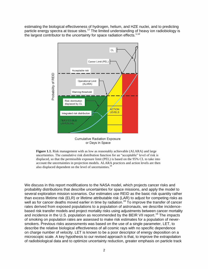
Exposures to astronauts from galactic cosmic rays (GCR) — made up of high-energy protons and high-energy and charge (HZE) nuclei, and solar particle events (SPEs) — that are comprised largely of low- to medium-energy protons are a critical challenge for space exploration. Experi-mental studies have shown that HZE nuclei produce both qualitative and quantitative differences in biological effects compared to terrestrial radiation,1-5 leading to large uncertainties in predicting exposure outcomes to humans. Radiation risks include carcinogenesis,6 degenerative tissue effects such as cataracts7,8 or heart disease,9-11 and acute radiation syndromes.6 Other risks, such as damage to the central nervous system (CNS), are a concern for HZE nuclei.1,5 For International Space Station (ISS) missions and design studies of exploration of the moon, near-Earth objects (NEOs), and Mars, NASA uses the quantity risk of exposure-induced death (REID) to limit astronaut risks. A REID probability of 3% is the criteria for setting age- and gender-specific exposure limits, while protecting against uncertainties in risk projection models is made using estimates of the upper 95% confidence level (CL). Risk projection models serve several roles, including: setting the age- and gender-specific exposure-to-risk conversion factors needed to define dose limits, projecting mission risks, and evaluating the effectiveness of shielding or other countermeasures. For mission planning and operations, NASA uses the model recommended in NCRP [National Council of Radiation Pro-tection and Measurements] Report No. 132 to estimate cancer risks from space.6 The model employs a life-table formalism to model competing risks in an average population, epidemiological assessments of excess risk in exposed cohorts such as the atomic-bomb survivors, and esti-mates of dose and dose-rate reduction factors (DDREFs) and linear energy transfer (LET)-dependent radiation quality factors (QFs) to estimate organ dose equivalents. NASA recognizes that projecting uncertainties in cancer risk estimates along with point estimates is an essential requirement for ensuring mission safety, as point estimates alone have limited value when the uncertainties in the factors that enter into risk calculations are large. Estimates of 95% confidence intervals (CI) for various radiation protection scenarios are meaning-ful additions to the traditional point estimates, and can be used to explore the value of mitigation approaches and research that could narrow the various factors that enter into risk assessments. Figure 1.1 illustrates the approach used at NASA as the number of days in space or an astro-naut’s career exposure accumulates. Because of the penetrating nature of the GCR and the buildup of secondary radiation in tissue behind practical amounts of all materials, we argued previously12-14 that improving knowledge of biological effects to narrow CI is the most cost-effective approach to achieve NASA safety goals for space exploration. Furthermore, this knowledge is essential to perform cost-benefit analysis of mitigation measures, such as shielding approaches and biological countermeasures, and to practice the safety require-ment embodied in the principle of as low as reasonably achievable (ALARA).

Uncertainties for low-LET radiation, such as -rays or x rays, have been reviewed several times in the past, and indicate that the major uncertainty is the extrapolation of cancer effects data from high to low doses and dose-rates.15,16 The (National Academy of Science [NAS]) Committee on the Biological Effects of Ionizing Radiation (BEIR) VII16 and United Nations Special Committee on the Effects of Atomic Radiation (UNSCEAR) committees17 recently provided new assessments of low-LET radiation risks. Uncertainties consist of the transfer of risk across populations and the sources of error in epidemiology data, including dosimetry, recording bias, and statistical errors. Probability distribution functions (PDFs), described previously,15 were used to estimate low-LET risk uncertainties. For space radiation risks, additional uncertainties occur related to

2

estimating the biological effectiveness of hydrogen, helium, and HZE nuclei, and to predicting particle energy spectra at tissue sites.12 The limited understanding of heavy ion radiobiology is the largest contributor to the uncertainty for space radiation effects.1,12

We discuss in this report modifications to the NASA model, which projects cancer risks and probability distributions that describe uncertainties for space missions, and apply the model to several exploration mission scenarios. Our estimates use REID as the basic risk quantity rather than excess lifetime risk (ELR) or lifetime attributable risk (LAR) to adjust for competing risks as well as for cancer deaths moved earlier in time by radiation.19 To improve the transfer of cancer rates derived from exposed populations to a population of astronauts, we describe incidence-based risk transfer models and project mortality risks using adjustments between cancer mortality and incidence in the U.S. population as recommended by the BEIR VII report.16 The impacts of smoking on population rates are assessed to make risk estimates for a population of never-smokers. Previous risks assessments was based on the use of a single parameter, LET, to describe the relative biological effectiveness of all cosmic rays with no specific dependence on charge number of velocity. LET is known to be a poor descriptor of energy deposition on a microscopic scale. A key hypothesis to our revised approach is that, to improve the extrapolation of radiobiological data and to optimize uncertainty reduction, greater emphasis on particle track

Figure 1.1. Risk management with as low as reasonably achievable (ALARA) and large

uncertainties. The cumulative risk distribution function for an “acceptable” level of risk is

displaced, so that the permissible exposure limit (PEL) is based on the 95% CL to take into

account the uncertainties in projection models. ALARA practices and action levels are then

also displaced dependent on the level of uncertainties.18

3

structure in describing energy deposition and subsequent biological events at the molecular, cellular, and tissue levels is required. We describe data and theoretical analysis that support the redefinition of radiation quality in terms of track structure parameters, and the assignment of distinct radiation QFs for solid cancer and leukemia with significantly lower values recommended for leukemia compared to solid cancer. The relationship between event- and fluence-based models and organ dose equivalent approaches is discussed.

1.1 Uncertainty Assessments and Classification The established approach to estimate uncertainties is to use Monte-Carlo simulations of subjective PDFs that represent current knowledge of factors that enter into risk assessments2,12,15,20 to propagate uncertainties across multiple contributors. We can write a risk equation in a simplified manner as a product of several factors including the dose, D, quality factor, Q, a low-LET risk coefficient normally derived from the data of the atomic-bomb survivors, R0, and the dose and dose-rate reduction effectiveness factor, DDREF, that corrects risk data for dose-rate modifiers. Monte-Carlo uncertainty analysis uses the risk equation, but the equation is modified by normal deviates that represent subjective weights and ranges of

values for various factors that enter into a risk calculation. First, we define XR(x) as a random variate that takes on quantiles x1, x2, …, xn such that p(xi) =P(X=xi) with the normalization

condition p(xi)=1. C(xi) is defined as the cumulative distribution function, C(x), which maps X into the uniform distribution U(0,1), and we define the inverse cumulative distribution function C(x)-1 to perform inverse mapping of U(0,1) into x: x=C(x)-1. Then we write for a simplified form

of the risk equation for a Monte-Carlo trial, :

0

0 ( , )

R

R phys Q

D

x x xFLQRisk R age gender

DDREF x

(1.1)

where R0 is the low-LET risk coefficient per unit dose, the absorbed dose, D, is written as the product of the particle fluence, F, and LET, L, and Q is the radiation QF. The xR, xphys, xDr, and xQ are quantiles that represent the uncertainties in the low-LET risk coefficient, space physics models of organ exposures, dose-rate effects, and radiation quality effects, respectively. Monte-Carlo trials are repeated many times, and resulting values are binned to form an overall PDF taking into account the model uncertainties. In this report, updates to the risk coefficients and QFs as well as and the revised PDFs for the various factors are described based on recent data and findings. In practice, the risk model does not use the simple form of Eq(1.1). Instead, risk calculations are based on a double-detriment life-table calculation that considers age, gender, and tissue-specific, radiation-induced cancer rates within a competing risk model with all causes of death in an average population.6,17

The model of Eq(1.1) and similar models make several important assumptions that we note here:

1) Risk assessments are population-based calculations that are applied to individuals rather than individual-based calculations. Legal and ethical obstacles to individual-based risk assessment are being described elsewhere along with the current scientific limitations to such approaches for low dose-rate exposures.21,22

2) A linear and additive response over each contribution of each particle to cumulative risk is assumed. The linearity and additivity of radiation component assumptions are em-bodied in the use of QFs, Q. QFs are subjective judgments of experimental determinations

4

of maximum relative biological effectiveness (RBE) factors determined as the ratio of initial

slopes for linear dose response curves for ions compared to -rays denoted as RBEmax.

Under this assumption, the DDREF applies only to -rays. No dependence of space radiation risks on dose-rate is presumed.

3) The risk model implicitly assumes that only quantitative differences between low- and high-LET radiation are important for risk assessment, thereby neglecting any impacts from qualitative differences.

The types of uncertainties that occur in cancer risk projection models can be classified as:

Type I Uncertainties: Uncertainties in human epidemiology data including statistical, record keeping, dosimetry, and bias. In addition, the shape of the dose-response curve such as linear, linear-quadratic and the possibility of dose thresholds are uncertainties in models of epidemiology data. Also, the role of confounders such as host environmental exposure, including smoke from tobacco products and dietary and genetic factors.

Type II Uncertainties: Uncertainties in application of radio-epidemiology data to other populations including transfer models, cancer rates and survival data in the population of interest, and differences due to individual variations in radiation sensitivity. For certain radiation workers, the effects of interactions with smoking are important. Due to the limitations in data for cancer rates above age 85-y extrapolation to older ages is important, especially for healthy workers who will enjoy significant increases in life span when not exposed to radiation compared to the average U.S. population.

Type III Uncertainties: Uncertainties in applying radio-epidemiology data to other radiation types and dose-rates including dose-rate and dose-protraction effects, radiation quality effects, and uncertainties in space dosimetry, which includes space environmental models, transport codes, and dosimetry methods.

Type IV Uncertainties: Type IV uncertainties include the possible inter-dependencies of the other Uncertainty classes (I to III). For example, if radiation quality leads to differences in transfer model assumptions including qualitative differences that would preclude the scaling of cancer risks using an RBE or similar quantity. In addition, assumptions about radiation sensitivity may be distinct at high versus low dose-rate, or depend on radiation quality.

The models described in this report describe some but not all of the Type I to IV uncertainties. Most importantly the effects of individual sensitivity (part of Type II uncertainties), and Type IV uncertainties are not described. In addition, the uncertainties due to extrapolation of population data for cancer rates beyond age 85-y have not been included at this time.

Ground-based research at the NASA Space Radiation Laboratory (NSRL) continues to document important quantitative and qualitative differences in the biological effects of HZE nuclei, including in the types of deoxyribonucleic acid (DNA) damages and chromosomal arrangements, gene expression, and signal transduction induced by radiation. Important differences between these processes at high vs. low doses have also been documented. Non-targeted effects (NTE), including bystander effects and genomic instability in the progeny of irradiated cells,23,24 are currently of great interest in radiation protection as they challenge the traditional paradigm of dose responses, which increase in a manner proportional to dose without threshold. These assumptions are clearly motivated by a DNA mutation mechanism or other targeted DNA effects (targeted effects [TE]). NTEs often are suggestive of qualitative differ-ences between low- and high-LET radiation. Ultimately, low-LET and simulated space radiation

5

can be compared for the same endpoint, such as overall cancer risk or tissue-specific cancer risks, albeit there are both qualitative and quantitative differences in causative steps leading to these endpoints. However, elucidation of the biological importance of quantitative differences through mechanistic research is essential for improving current risk models. A long-time out-standing question is the use of dose-based models to describe cosmic-ray tracks as they pass through tissue. Figure 1.2 illustrates some of the differences between dose-based risk models and particle track structure. Quantitative and qualitative differences occur, and the use of radiation QFs may not be justified in all or certain cases.

NASA radiation protection methods are based on recommendations issued by the NCRP6,25 and the International Commission on Radiological Protection (ICRP),26 but independent approaches have been developed and continue to be developed that lead to better implementation in the context of space exploration. In those instances, details of NASA practice differ from these recommendations. For example, NASA uses cancer-mortality-based career limits rather than limits that are based on overall health detriment, as recommended by the ICRP, and gender-specific career limits calculated for individual astronaut mission exposure histories rather than attained age. Distinct short-term limits are followed originating in recommendations from the National Research Council (NRC) (1970). NASA continued to use Q(L) (ie, QF as a function of LET) rather than ICRP radiation weighting factors based on NCRP recommendations,6,25 and also uses distinct RBEs for non-cancer risks instead of the QFs employed in estimating cancer risks. NASA estimates the 95% CLs as a requirement for dose limits, and recently considered limits for the CNS and heart disease.27 Dosimetry28 and ALARA implementation for space

Figure 1.2. A comparison of particle tracks in nuclear emulsions and human cells. The right

panel illustrates tracks of different ions, from protons to iron, in nuclear emulsions, clearly

showing the increasing ionization density (LET=E/x) along the track by increasing the

charge Z. The left panel shows three nuclei of human fibroblasts exposed to -rays and Si- or

Fe-ions, and immunostained for detection of -H2AX P14 P. Each green focus corresponds to a

DNA double-strand break (DSB). Whereas the H2AX foci in the cell that is exposed to

sparsely ionizing -rays are uniformly distributed in the nucleus, the cells that are exposed to

HZE particles present DNA damage along tracks (one Si- and three Fe-particles, respectively),

and the spacing between DNA DSB is reduced at very high LET.2

6

missions, including the timing of spacewalks,29 and operational biodosimetry30 also distinguish NASA procedures from terrestrial radiation protection procedures. Whereas the revised approach described in this report for space radiation cancer risk assessments leads to additional modifications from prior methods recommended by NCRP or ICRP, it is nevertheless consistent with the overall principles of NCRP and ICRP because the higher risk levels of long-term space missions require more accurate assessments than are used in most ground-based scenarios. To quote the ICRP from its recent assessment of QFs:31

“Accurate determinations may seem to be an academic issue in radiation protection. Under routine circumstances, where exposures are substantially below the limits, this is indeed the case. Then there is no need for accurate assessments. However, in radiological protection, as in other formally adopted and legally binding protection or safety systems, a limit must also be rigorously defined quantity because exposures must, in certain critical cases, be assessed accurately. Looseness that can involve uncertainties by a factor of 2 or more is tolerable under many routine conditions, but it will make the system inoperable in exactly those critical circumstances where compliance with regulatory limits is in question and must be reliably quantified.” [p. 68, para. 230]

Thus, the required accuracy for radiation projection for long-term space travel makes many of the methodologies recommended by the ICRP and the NCRP inadequate for NASA. However, the approach described in the present report is consistent with the NCRP overall recommended principles of risk justification, risk limitation, and ALARA. In the final section of this report, we will discuss predictions for space missions as well as changes to dosimetry and computer codes procedures that result from our recommended changes to the NASA cancer projection model.

1.2 Basic Concepts Radiation exposures are often described in terms of the physical quantity absorbed dose, D, which is defined as the energy deposited per unit mass. Dose has units of Joule/kg that define the special unit, 1 Gray (Gy), which is equivalent to 100 rad (1 Gy = 1 rad). In space, each cell within an astronaut is exposed every few days to a nuclear particle that comprises the GCR. The GCR is the nuclei of atoms accelerated to high energies in which the atomic electrons are stripped off. It is common to discuss the number of particles per unit area, called the fluence, F, with units of 1/cm2. As particles pass through matter, they lose energy at a rate dependent on their kinetic energy, E, and charge number, Z, and approximately the average ratio of charge to mass, (ZT/AT) of the materials they traverse. The rate of energy loss is called the LET, which, for

unit density materials such as tissue, is given in units of keV/m. Dose and fluence are related

by D = F LET, where is the density of the material (eg, 1 g/cm3 for water or tissue). The dependence of energy loss on the ZT/AT ratio implies that hydrogen, with its ratio equal to 1, is the optimal material for slowing particles. There is a broad energy range for the cosmic rays,

and the spectra of particles is denoted as the fluence spectra, j(E), where j refers to the particle type described by Z and the mass number, A. The particle velocity scaled to the speed of light,

denoted as , is related to the kinetic energy. E and are related using the formula =1 + E/m

where m is the nucleon rest mass (938 MeV) and =(1-1/2)-1/2. Kinetic energies are often ex-pressed in units of MeV per atomic mass unit (u), MeV/u because particles with identical E

then have the same . The total kinetic energy of the particle is then A times E.

7

The GCR of interest has a charge number, Z from 1 to 28, and energy from less than 1 MeV/u to more than 10 000 MeV/u with a median energy of about 1000 MeV/u. The GCR with energies less than about 2000 MeV/u is modulated by the 11-y solar cycle, with more than two times higher GCR flux at solar minimum when the solar wind is weakest compared to the flux at solar maximum. The most recent solar minimum was in 2008-2009, and the next will occur in about 2019. SPEs occur about 5 to 10 times per year, except near solar minimum, and consist largely of protons with kinetic energies below 1 MeV up to a few hundred MeV. However, most SPEs lead to small doses (<0.01 Gy) in tissue; and only a small percentage (<10%) would lead to significant health risks if astronauts were not protected by shielding. At this time, there is very little capability to predict the onset time and determine whether a large or small SPE will occur until many hours after an SPE has commenced. Mission disruption may occur for many SPEs, although the health risks are very small. Nuclear and atomic interactions in materials are best described using the material thickness, x,

described as an areal density, t = x, where is the atomic density of the material with values

for common materials of = 1.0, 2.7, and 0.96 for tissue, aluminum, and high-density polyeth-ylene, respectively. The range of a particle is defined as the average distance traveled before the particle loses all of its kinetic energy and stops. The range increases with E and is a few g/cm2 at 50 MeV/u, and more than 100 g/cm2 at 1000 MeV/u. Nuclear reactions, which occur through interactions of cosmic rays with the nuclei of atoms in shielding materials or tissue, lead to the production of secondary radiation, including neutrons and charged particles from the atoms of the shielding material or tissue. The mean free path for a nuclear reaction increases with the mass of the cosmic ray; about 10 g/cm2 for heavy nuclei such as iron (A=56; Z=26), and more than 20 g/cm2 for protons (A=1; Z=1). Shielding thickness of 10 to 20 g/cm2 is sufficient to protect against most SPEs; however, thicknesses of several hundred g/cm2 are needed to significantly reduce organ doses from GCR, making shielding impractical as an efficient method of protection. Energy loss by cosmic rays occurs through ionization and excitation of target atoms in the shielding material or tissue. The ionization of atoms leads to the liberation of electrons that often have sufficient energy to cause further excitations and ionizations of nearby target atoms. These

electrons, which are called -rays, can have energies more than 1 MeV for ions with E>1000

MeV/u. About 80% of the LET of a particle is due to ionizations leading to -rays. The number of

-rays created is proportional to Z*2/2, where Z* is the effective charge number that adjusts Z by

atomic screening effects important at low E and high Z. The lateral spread of -rays, called the

track-width (illustrated in Figure 1.2) of the particle, is dependent on but not on Z being deter-

mined by kinematics. At 1 MeV/u, the track-width is about 100 nm (0.1 m); and at 1000 MeV/u, the track-width is about 1 cm. A phenomenological approach to describing atomic ionization and excitation is to introduce an empirical model of energy deposition. Some definition of a charac-teristic target volume is needed to apply this model. A diverse choice of volumes is used in radiobiology, including volumes with diameters <10 nm to represent short DNA segments, and of diameters from a few to 10 microns to represent cell nuclei or cells. Energy deposition is the sum of energy transfer events due to ionizations and excitations in the volume including those

from -rays. For large target volumes, energy deposition and energy loss (LET) become approx-imately the same. Two particles with different Z and identical LET will have different values for E and, therefore, different track-widths. The particle with lower Z will have a narrower track-width and more localized energy deposition, and in many experiments has been shown to have a higher biological effectiveness than a particle with higher Z. In tissue, however, the higher Z nuclei often have a larger range and can traverse more cell layers than the lower Z nuclei at the same LET.

8

The biological effects of different types of particles are usually compared using the ratio of doses that leads to an identical effect. This ratio is called the RBE factor. Human data for low-

LET radiation, such as -ray or x-ray exposures leading to increased cancer risk, have been studied in the survivors of the atomic bombs in Japan during World War II, medical patients exposed therapeutically to radiation, and nuclear reactor works. However, there are no human data for high-LET radiation such as cosmic rays with which to make risk estimates. Therefore,

RBEs in which the dose in the numerator is that of -rays and the dose in the denominator of a nuclear particle being studied, are often used to compare results from biological experiments with nuclei created at particle accelerators to the results of epidemiological studies in humans

exposed to -rays or x rays. RBEs vary widely with the biological endpoint, cell or animal system, type of radiation, and doses used in experiments. Traditionally, it has been the role of advisory panels to make a subjective judgment of available RBE data to make estimates for human risk. Such judgment is used to define a radiation QF. For terrestrial radiation exposures QFs, Q has been defined uniquely by LET, Q(LET). Values of Q from 1 to 30 have been used in the past for

different LET values with Q=1 below 10 keV/m and Q=30 at 100 keV/m used at this time. For the more complex radiation environments in space, however, the inaccuracy of LET as a descriptor of biological effects has been a long-standing concern. Multiplication of the absorbed dose by the QF is referred to as the dose equivalent, H = Q(LET) D, which has units denoted as 1 Sv (1 Sv = 100 rem; of 1 mSv = 0.1 rem). For calculating cancer risks, radiation transport codes are used to describe the atomic and nuclear collisions that occur inside spacecraft and tissue. Resulting particle spectra, averaged over the tissues of concern for cancer risk (eg, lung, stomach, colon, bone marrow, etc.), are used to describe the organ dose equivalent, HT. Because human epidemiological data are predominantly for high dose-rates, methods to estimate cancer risks at low dose-rates are needed. The traditional approach to this problem has been to estimate a DDREF that reduces the high dose-rate risk estimate for its application to low dose and dose-rates. DDREF values from 1.5 to 2.5 have been recommended in the past. The use of radiation QFs and DDREFs is a major concern for space radiation risks because there are both quantitative and qualitative differences observed in experimental systems of cancer risks. It is unclear whether these quantities are sufficiently accurate to form a basis for risk estimates. NASA limits astronaut cancer risks to a lifetime REID of 3%. Because long space missions are projected to approach and exceed this risk limit, uncertainty analyses of the models and methods used to make risk estimates are performed, including values and descriptions of HT, Q, and DDREF, which is the focus of this report.

9

2. Space Radiation Environments and Transport Models

In this chapter, we review models of the space radiation environments and organ exposures as well as recent developments in their physical characterization in support of human missions. To characterize uncertainties in physics models of space radiation the kinetic energy (E), mass number (A), and charge number (Z), the dependent fluence distribution F(E,A,Z) behind space-craft and tissue shielding must be evaluated. The space physics uncertainty for estimating particle fluence distributions, F(E,A,Z), at tissues of interest behind shielding has three components: space environments(xenv), radiation transport(xtran), and spacecraft and tissue shielding de-

scriptions (xshield). Overall uncertainties contributing to Monte-Carlo trial, can be written as:

( , , ) ( , , )M env tran shieldF E A Z F E A Z x x x (2.1)

where FM is a baseline model for the fluence distribution at sensitive tissues that is being estimated. We review each of these factors in the current chapter. There are also variability considerations to be addressed when considering organ exposures from space radiation. These variables include: orientation of crew members inside a vehicle, peculiarities of an individual’s size and composition relative to the standard human geometry model used in calculations or perhaps phantom measurements, or the exact position in which a crew member’s dosimetry is worn. Variability analysis can be made, employing similar methods to those used here for uncertainty analysis,32 and considered in future reports. The types and energies of particle radiation in space are summarized in Figure 2.1. The predominant types of particle radiation in the Earth environment are solar flare protons, trapped protons and electrons, and GCR. There are temporal variations as well as spatial distributions for each radiation source.

Figure 2.1. Schematic of energy ranges of space radiation environments.

33

10

It is convenient to consider the particulate radiation in space as arising from these distinct sources as defined by their location: the solar particle radiation, the GCR, and the trapped particle radiation. We consider models of GCR and SPE next. The trapped radiation makes no contribution outside of low-Earth orbit (LEO) and only a very minor contribution for ISS organ exposures because here GCR dominates, representing more than 80% of organ dose equiv-alents.30,34 The uncertainties in the trapped environments are not described here.

2.1 Galactic Cosmic Ray Models The GCR pervades the near-Earth environment omnidirectionally, and has a range of energies that exceeds 10 GeV/u. The GCR consists of fully ionized nuclei because the electrons are stripped from the atoms during the acceleration of ions to high energies. Most cosmic rays prob-ably originate in our galaxy, especially in supernova explosions,35,36 although the highest energy

components (1017 eV amu-1) may be of extragalactic origin.37 The region outside the solar sys-tem in the outer part of the galaxy is believed to be filled uniformly with GCR. The GCR nuclei constitute approximately one third of the energy density of the interstellar medium and, on a galactic scale, form a relativistic gas whose pressure is important to take into account in the dy-namics of galactic magnetic fields. GCR nuclei are the only direct and measurable sample of matter from outside the solar system. It is a unique sample since it includes all of the elements, from hydrogen to the actinides. The GCR arriving beyond the Earth magnetic field at the distance of the Earth from the sun (1 AU [astronomical unit]) is composed of approximately 98% nuclei and approximately 2% electrons and positrons.38 In the energy range 108 to 1010 eV/u, where it has its highest intensity, the nuclear component consists roughly of 87% protons, approximately 12% helium nuclei, and a total of approximately 1% for all heavier nuclei from carbon to the actinides.38 Although GCR probably include every natural element, not all GCR are important for space radiation protection purposes. The elemental abundances for species heavier than iron (atomic charge number Z > 26) are typically 2 to 4 orders of magnitude smaller than the elemental abundance for iron.38 Some elements such as the L nuclei (Li, Be, B), F, and several nuclei between Si and Fe are quite rare38,39 in the solar system; whereas, in the GCR flux, nuclei of these elements are present nearly as commonly as those of their neighbors. This shows that the GCR originates in the breakup of heavy particles during GCR propagation, which would not be present in the GCR at stellar sources.40,41

Experimental studies of high-charge (Z) and energy (E) nuclei (HZE) were made on the Pioneer, Voyager, and Ulysses spacecraft to measure the isotopic composition of GCR ele-ments near Earth and in deep space.40,42-47 In recent years, the Advanced Composition Explorer (ACE) has made substantial contributions to our understanding of GCR composition and solar modulation.48 Data of the GCR and SPE near Mars were also collected by the Martian Radia-tion Environment Experiment [MARIE] on the Mars Odyssey spacecraft.49

2.1.1 Model of galactic cosmic rays charge and energy spectra

Badhwar and O’Neill50 have developed a self-consistent solution to the Fokker-Plank equation for particle transport in the heliosphere that has been fit to available GCR data. This model accurately accounts for solar modulation of each element (hydrogen through nickel) by propagating the local interplanetary spectrum (LIS) of each element through the heliosphere by solving the Fokker-Planck diffusion, convection, and energy loss boundary value problem. A

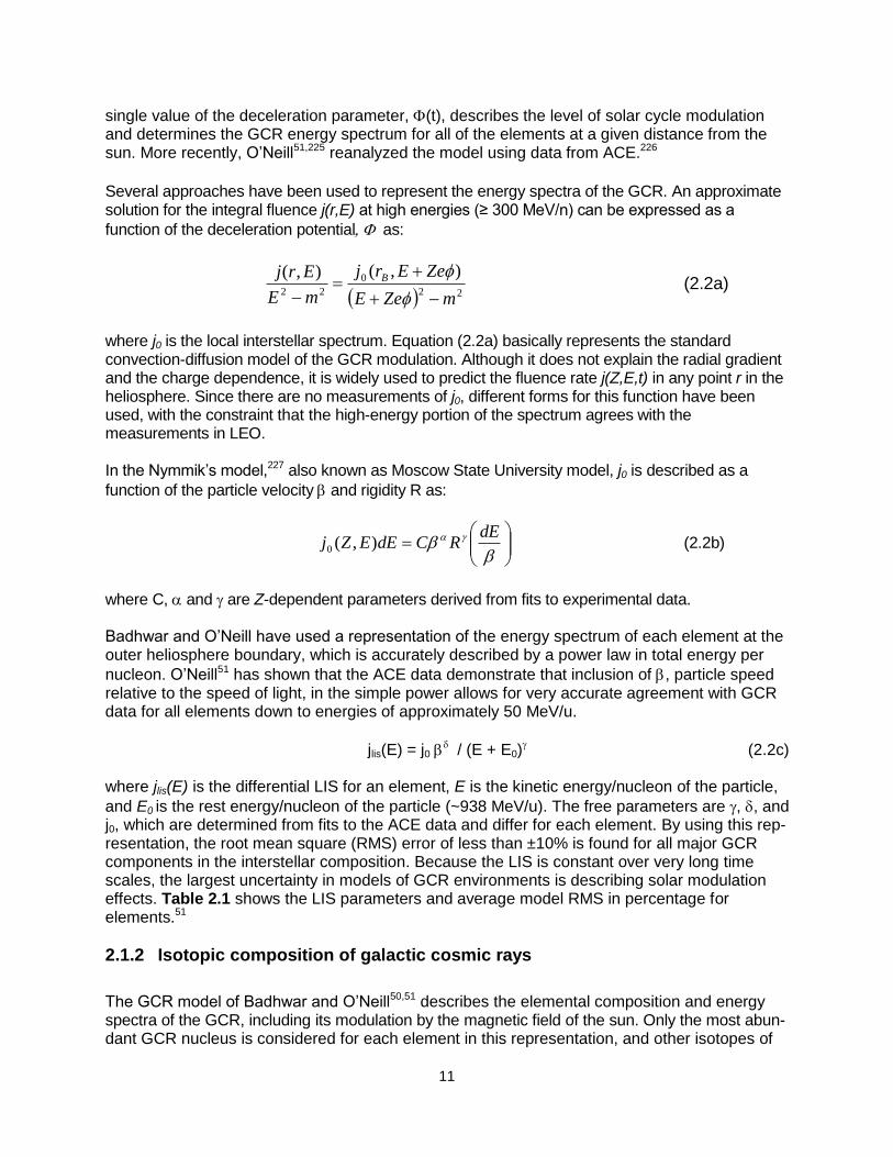
11

single value of the deceleration parameter, (t), describes the level of solar cycle modulation and determines the GCR energy spectrum for all of the elements at a given distance from the sun. More recently, O’Neill51,225 reanalyzed the model using data from ACE.226

Several approaches have been used to represent the energy spectra of the GCR. An approximate solution for the integral fluence j(r,E) at high energies (≥ 300 MeV/n) can be expressed as a

function of the deceleration potential as:

22

0

22

),(),(

mZeE

ZeErj

mE

Erj B

(2.2a)

where j0 is the local interstellar spectrum. Equation (2.2a) basically represents the standard convection-diffusion model of the GCR modulation. Although it does not explain the radial gradient and the charge dependence, it is widely used to predict the fluence rate j(Z,E,t) in any point r in the heliosphere. Since there are no measurements of j0, different forms for this function have been used, with the constraint that the high-energy portion of the spectrum agrees with the measurements in LEO. In the Nymmik’s model,227 also known as Moscow State University model, j0 is described as a

function of the particle velocity and rigidity R as:

dE

RCdEEZj ),(0 (2.2b)

where C, and are Z-dependent parameters derived from fits to experimental data. Badhwar and O’Neill have used a representation of the energy spectrum of each element at the outer heliosphere boundary, which is accurately described by a power law in total energy per

nucleon. O’Neill51 has shown that the ACE data demonstrate that inclusion of , particle speed relative to the speed of light, in the simple power allows for very accurate agreement with GCR data for all elements down to energies of approximately 50 MeV/u.

jlis(E) = j0 / (E + E0)

(2.2c)

where jlis(E) is the differential LIS for an element, E is the kinetic energy/nucleon of the particle,

and E0 is the rest energy/nucleon of the particle (~938 MeV/u). The free parameters are , , and j0, which are determined from fits to the ACE data and differ for each element. By using this rep-resentation, the root mean square (RMS) error of less than ±10% is found for all major GCR components in the interstellar composition. Because the LIS is constant over very long time scales, the largest uncertainty in models of GCR environments is describing solar modulation effects. Table 2.1 shows the LIS parameters and average model RMS in percentage for elements.51

2.1.2 Isotopic composition of galactic cosmic rays

The GCR model of Badhwar and O’Neill50,51 describes the elemental composition and energy spectra of the GCR, including its modulation by the magnetic field of the sun. Only the most abun-dant GCR nucleus is considered for each element in this representation, and other isotopes of

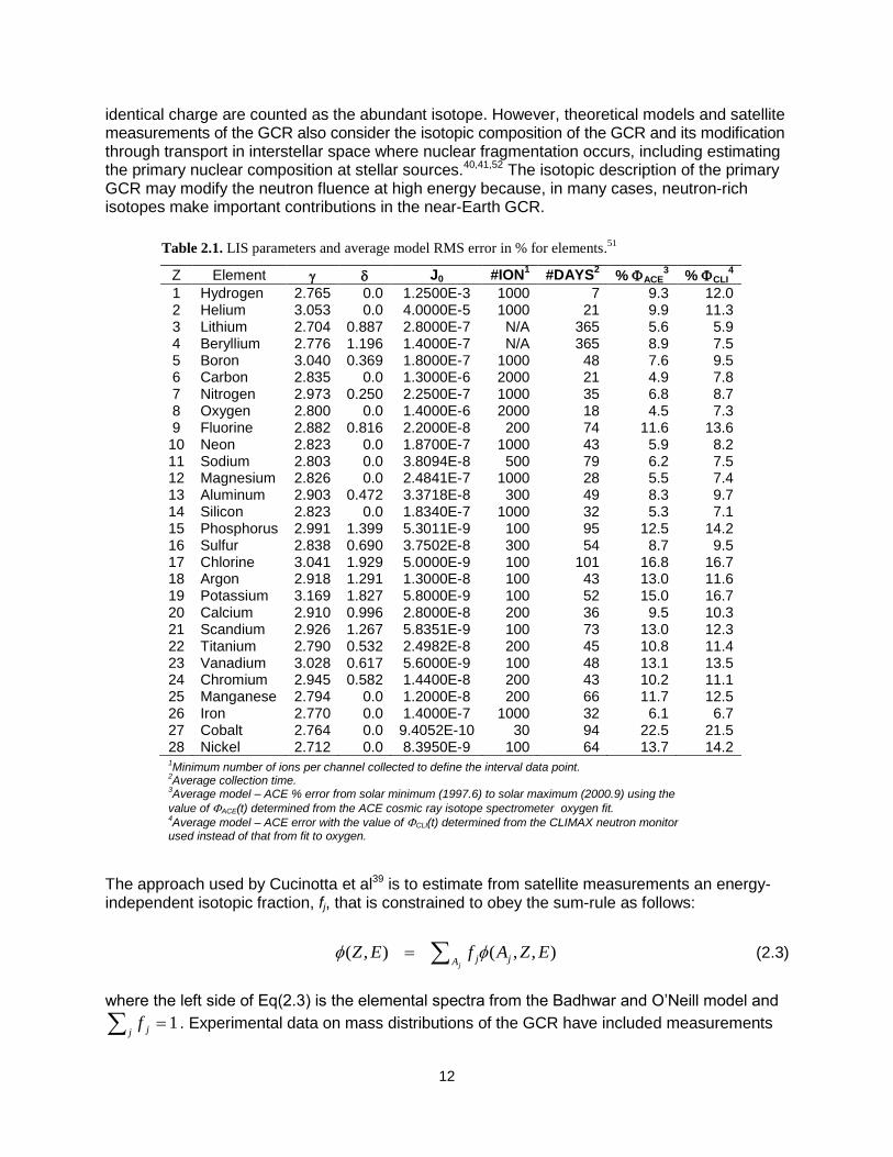
12

identical charge are counted as the abundant isotope. However, theoretical models and satellite measurements of the GCR also consider the isotopic composition of the GCR and its modification through transport in interstellar space where nuclear fragmentation occurs, including estimating the primary nuclear composition at stellar sources.40,41,52 The isotopic description of the primary GCR may modify the neutron fluence at high energy because, in many cases, neutron-rich isotopes make important contributions in the near-Earth GCR.

The approach used by Cucinotta et al39 is to estimate from satellite measurements an energy-independent isotopic fraction, fj, that is constrained to obey the sum-rule as follows:

( , ) ( , , )j

j jAZ E f A Z E (2.3)

where the left side of Eq(2.3) is the elemental spectra from the Badhwar and O’Neill model and

j jf 1 . Experimental data on mass distributions of the GCR have included measurements

Table 2.1. LIS parameters and average model RMS error in % for elements.51

5BZ 6BElement 0BJ0 1B#ION1

2B#DAYS2

3B% ACE3

4B% CLI4

1 Hydrogen 2.765 0.0 1.2500E-3 1000 7 9.3 12.0 2 Helium 3.053 0.0 4.0000E-5 1000 21 9.9 11.3 3 Lithium 2.704 0.887 2.8000E-7 N/A 365 5.6 5.9 4 Beryllium 2.776 1.196 1.4000E-7 N/A 365 8.9 7.5 5 Boron 3.040 0.369 1.8000E-7 1000 48 7.6 9.5 6 Carbon 2.835 0.0 1.3000E-6 2000 21 4.9 7.8 7 Nitrogen 2.973 0.250 2.2500E-7 1000 35 6.8 8.7 8 Oxygen 2.800 0.0 1.4000E-6 2000 18 4.5 7.3 9 Fluorine 2.882 0.816 2.2000E-8 200 74 11.6 13.6 10 Neon 2.823 0.0 1.8700E-7 1000 43 5.9 8.2 11 Sodium 2.803 0.0 3.8094E-8 500 79 6.2 7.5 12 Magnesium 2.826 0.0 2.4841E-7 1000 28 5.5 7.4 13 Aluminum 2.903 0.472 3.3718E-8 300 49 8.3 9.7 14 Silicon 2.823 0.0 1.8340E-7 1000 32 5.3 7.1 15 Phosphorus 2.991 1.399 5.3011E-9 100 95 12.5 14.2 16 Sulfur 2.838 0.690 3.7502E-8 300 54 8.7 9.5 17 Chlorine 3.041 1.929 5.0000E-9 100 101 16.8 16.7 18 Argon 2.918 1.291 1.3000E-8 100 43 13.0 11.6 19 Potassium 3.169 1.827 5.8000E-9 100 52 15.0 16.7 20 Calcium 2.910 0.996 2.8000E-8 200 36 9.5 10.3 21 Scandium 2.926 1.267 5.8351E-9 100 73 13.0 12.3 22 Titanium 2.790 0.532 2.4982E-8 200 45 10.8 11.4 23 Vanadium 3.028 0.617 5.6000E-9 100 48 13.1 13.5 24 Chromium 2.945 0.582 1.4400E-8 200 43 10.2 11.1 25 Manganese 2.794 0.0 1.2000E-8 200 66 11.7 12.5 26 Iron 2.770 0.0 1.4000E-7 1000 32 6.1 6.7 27 Cobalt 2.764 0.0 9.4052E-10 30 94 22.5 21.5 28 Nickel 2.712 0.0 8.3950E-9 100 64 13.7 14.2 1Minimum number of ions per channel collected to define the interval data point.

2Average collection time.

3Average model – ACE % error from solar minimum (1997.6) to solar maximum (2000.9) using the

value of ACE(t) determined from the ACE cosmic ray isotope spectrometer oxygen fit. 4Average model – ACE error with the value of CLI(t) determined from the CLIMAX neutron monitor

used instead of that from fit to oxygen.

13

on the Pioneer, Voyager, and Ulysses spacecraft. Since secondary fragment production is mod-ulated by the transit time in the heliosphere, the isotopic fraction is dependent on the position in the solar cycle. However, we compared radiation shielding calculations in which the isotopic com-ponents were modulated over the solar cycle to calculations fixed by the Ulysses estimates near solar minimum and found the differences to be small. The Ulysses estimates are then used for the isotopic composition for radiation transport calculations, such as with the HZETRN code.39

For the Z=1 and Z=2 ions, the following empirical formula can be used to estimate the primary (near-Earth) 2H and 3He spectra:39

Figure 2.2b. Energy spectra near solar minimum (=428 MV) for primary GCR isotopes of

Ne, Si, and Fe.

Figure 2.2.a. Energy spectra near solar minimum (=428 MV) and solar maximum (=1050

MV) for primary GCR light ions.

14

2

3 4( ) 0.0764 0.097exp[ 0.5(ln( /1660) /1.306) ] ( )He HeE E E (2.4a)

2 4( ) 0.2 ( )H He

E E (2.4b)

where 3He(E) is subtracted from the Badhwar and O’Neill model spectra for 4He(E). Primary 3H and neutron spectra are not considered because of their short half-lives. Examples of the GCR energy spectra for hydrogen and helium are shown in Figure 2.2a and for the isotopes of Ne, Si, and Fe at solar minimum in Figure 2.2b.

2.1.3 Solar modulation of the galactic cosmic rays

The intensity of the GCR flux varies over the approximately 11-y solar cycle due to changes in the interplanetary plasma that originates in the expanding solar corona.50,53 The intensity and energy of GCR entering the heliosphere is lowered as the rays are scattered by irregularities in the interplanetary magnetic field embedded in the solar wind. Parker52 showed that the steady-state, spherically symmetric Fokker-Planck equation accurately accounts for diffusion, convec-tion, and adiabatic deceleration of these particles.

If U is the cosmic ray density, E the particle kinetic energy, V the velocity, and the symmetric part of the diffusion tensor, the basic equation is52:

)5.2(013

1)( aUE

mE

m

EVUVU

t

U S

where m is the proton rest mass. A full numerical solution of the equation is given by the

deceleration potential (in MV):

'),'(

),'(

3

1),( dr

tr

trVtr

Br

r

w

(2.5b)

where rB is the radial extent of the heliosphere, the diffusion coefficient and Vw the solar wind velocity. The deceleration potential is the most important parameter in describing the modulation of

GCR intensity. The Fokker-Planck equation is readily solved numerically to propagate the LIS for each element to a given radius from the sun. A single diffusion coefficient, Eq(2.6), was used by Badhwar and O’Neill as well as by others to describe the effect of the magnetic field of the sun on particles entering the heliosphere.

k(r,t)=(k0/VSW)P[1+(r/r0)2]/(t)) (2.6)

where VSW is the constant solar wind speed (400 km/s), r is distance from the sun in AU, t is time

in years, k0 is constant, is particle speed relative to the speed of light, P is particle rigidity in MV,

and (t) is solar modulation parameter in MV.

15

In the Badhwar and O’Neill model the effect of magnetic field, including disturbances and the radial gradient, is described by the diffusion coefficient. An inverse square law (for 1/k(r, t)) for a spherical cavity is assumed. To fit each of the various elements from hydrogen to nickel with the simple analytical LIS form, the modulation cavity scaling parameter r0 was set to be 4.0 AU by O’Neill.51 The physical significance of the 4 AU cavity scaling is not yet clear; the actual boundary of the cavity was set at 50 AU. The single-fit parameter that determines the level of solar modu-

lation is k0/(t). O’Neill51 and others set k0 to a constant (k0 = 1.61021 cm2/s) and then deter-

mined the value of (t) that fits the measured spectra. The (t) is related to the energy and rigidity required for interstellar particles to propagate through the heliosphere to the radius of interest. The modulation parameter at solar minimum or maximum varies to some extent for each solar cycle.54 A worst-case solar minimum, based on the BO96 model of the 1977 minimum, has been widely used for shielding design studies. The most recent solar minimum (2009) was reported as significantly deeper compared to the 1977 solar minimum. For solar maximum a wide range of modulation parameters values is observed for each cycle; and, more importantly, the occurrence of large SPEs is not well predicted relative to the position in the solar cycle as described below. Therefore, a modulation parameter of about 1100 MV provided a reasonable GCR background to investigate SPE risks in the BO96 model. Recently, O’Neill (O’Neill et al, to be published) has modified the BO10 model225 to include a better representation of the GCR modulation as it relates to the smoothed mean sunspot number, and to improve the overall fit of the model to the historical GCR energy spectra, more recent HZE particle data from ACE, and the Interplanetary Monitoring Platform (IMP) data for protons and helium. The revised model is denoted at the BO11 model (O’Neill et al, to be published). In this model, a new feature is to introduce a modulation parameter for protons (Z=1) distinct from other GCR particles (Z>1). The description of the solar cycle considers two temporal progressions: 1) Pointed period during B- magnetic field where there is an immediate response to new solar cycle with minimal delay. 2) Plateau period during B+ magnetic field where there is a rapid GCR rise followed by a delayed decline. For protons, the relationship between sunspot number and the modulation is identical in the Pointed and Plateau periods. For Z>1 particles, a distinction is made leading to a different lag time. Figures 2.3 to 2.6 show representative results of the BO11 model for the modulation parameter based on the smoothed average sunspot number and comparisons of proton, helium, and iron particle predictions to various data sets.228-231 From these data, Table 2.2 shows calculations of average modulation parameter at solar min, solar max, and worst and best cases. Defining a worst-case GCR environment for mission design studies entails several considerations. We note that most NASA design studies have used a GCR environment representing the 1977 solar minimum to correspond to the worst case. Each solar cycle will have a distinct solar modulation and will depend on the polarity of the solar field, which itself switches from positive to negative polarity on a 22-y cycle. Negative polarity cycles are more likely to show deeper solar minima (smaller modulation parameters). As mission length increases, using a single-modulation parameter would overestimate the conditions at solar minimum. In our previous report we showed that the GCR modulation averaged over increasing mission length, and described the impact of using a fixed-modulation parameter.55 Solar modulation over recent cycles does not reflect historical periods. Castagnoli et al56 made estimates based on a sunspot number that suggests much deeper minima in past centuries. The effect of increased modulation beyond that of a recent solar minimum decreases with increasing shielding depth, perhaps

16

representing a 10% increase in GCR organ dose equivalents when comparing 428 MV to, say, 350 MV based on our earlier analysis.57

Figure 2.4. Comparison of BO11 model to recent balloon spectrometer data for proton and helium spectra

(O’Neill et al., 2012) .

0.0E+00

5.0E+05

1.0E+06

1.5E+06

2.0E+06

2.5E+06

3.0E+06

3.5E+06

4.0E+06

4.5E+06

5.0E+06

5.0E+00 5.0E+01 5.0E+02 5.0E+03 5.0E+04 5.0E+05

E x

(E),

1/(

cm2-y

r)

E, MeV/n

Helium Flux (Measurement vs BO11 GCR Model)

PAMELA_He

CAPRICE

BESS

IMAX (1992)

Avg_2006-8 (Phi=554 MV)

Aug. 9,1994 (Phi=491 MV)

July 29, 1998 (Phi=519 MV)

July 16, 1992 (Phi=605 MV)

0.0E+00

5.0E+06

1.0E+07

1.5E+07

2.0E+07

2.5E+07

3.0E+07

3.5E+07

4.0E+07

4.5E+07

5.0E+00 5.0E+01 5.0E+02 5.0E+03 5.0E+04 5.0E+05

E x

(E),

1/(

cm2-y

r)

E, MeV/n

Proton Flux (Measurement vs BO11 GCR Model)

PAMELA

CAPRICE

BESS_p

IMAX (1992)

Avg_2006-8 (Phi=554 MV)

Aug. 9, 1994 (Phi=557 MV)

July 29, 1998 (Phi=611 MV)

July 16, 1992 (Phi=777 MV)

Figure 2.3. BO11 model for GCR solar modulation parameter versus time compared to ACE and IMP derived

values. Results show distinct modulation values for protons compared to other particles.

400

600

800

1000

1200

1400

1600

1800

1950 1960 1970 1980 1990 2000 2010 2020

Ph

i, M

V

Time

Phi(Z=1), MV

Phi(Z>1), MV

IMP

ACE

Plateau Peak Plateau Peak Plateau Peak Plateau

17

Figure 2.5. Comparison of BO11 modulation of GCR iron fluence to ACE data for recent times.

0.0E+00

2.0E-04

4.0E-04

6.0E-04

8.0E-04

1.0E-03

1999 2001 2003 2005 2007 2009 2011 2013

Par

ticl

es/

(m2 -s

r-s-

MeV

/n)

Time

BO11 (284 - 432 MeV/n) ACE (270 - 450 MeV/n) ACE/Bartol Rotation (286.8 -465.9 MeV/n)

Previous space agerecord high

Table 2.2. Solar modulation parameters in BO11 model based on historical data smoothed average

sunspot numbers from 18th

century through 2011. The average solar min, solar max, and deepest and

weakest modulation parameters are shown for Z=1 and Z>1 particle modulation.

Modulation Condition Z=1 Z>1

Deep Sol Min 2009 (99th-percentile

or worse-case)

420 420

95th

Percentile 433.3 427.9

Ave. Sol Min 463.3 455.6

Median Solar Cycle 657.6 580.2

Ave. Sol. Max 924.3 817.5

10th

Percentile 1057.9 941.7

Deepest Solar Max 1740.9 1576.9

18

2.2 Solar Particle Events The origin of solar flares, coronal mass ejections (CMEs), etc., are discussed in a recent NCRP Report.5 For radiation protection purposes only, SPEs with integral 30 MeV proton fluences greater than 107 per cm2 are of importance. Radiation protection from SPEs can be divided into the pre-mission design phase and real-time responses during the mission (not discussed herein). The SPE frequency and total particle fluence, energy spectra, and duration must be described for mission design assessments. A solar flare is an intense local brightening on the face of the sun close to a sunspot. The solar abnormality results in an alteration of the general outflow of solar plasma at moderate energies and local solar magnetic fields carried by that plasma. An

Figure 2.6. GCR modulation parameters in BO11 model at solar min or solar max versus time (left panels) and

percentiles based on resulting values from 1750 to 2011 (right panels) for Z=1 and Z>1.

400

600

800

1000

1200

1400

1750 1800 1850 1900 1950 2000

Z

=1, M

V

Time

Solar Minimum Solar Maximum

400

600

800

1000

1200

1400

1750 1800 1850 1900 1950 2000

Z

>1, M

V

Time

Solar Minimum Solar Maximum

0%

10%

20%

30%

40%

50%

60%

70%

80%

90%

100%

400 600 800 1000 1200 1400 1600

Pe

rce

nti

le

Monthly Average Z>1, MV

Combined Distribution of Monthly Z>1 for All Cycles

0%

10%

20%

30%

40%

50%

60%

70%

80%

90%

100%

400 600 800 1000 1200 1400 1600 1800

Pe

rce

nti

le

Monthly Average Z1, MV

Combined Distribution of

Monthly Z=1 for All Cycles

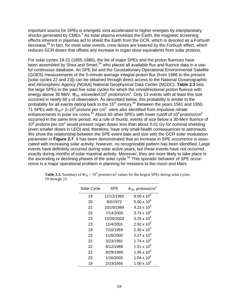
19

important source for SPEs is energetic ions accelerated to higher energies by interplanetary shocks generated by CMEs.5 As solar plasma envelops the Earth, the magnetic screening effects inherent in plasmas act to shield the Earth from the GCR, which is denoted as a Forbush decrease.58 In fact, for most solar events, crew doses are lowered by the Forbush effect, which reduces GCR doses that offsets any increase in organ dose equivalents from solar protons.

For solar cycles 19-21 (1955-1986), the list of major SPEs and the proton fluences have been assembled by Shea and Smart,59 who placed all available flux and fluence data in a use-ful continuous database. An SPE list and the Geostationary Operational Environmental Satellite (GOES) measurements of the 5-minute average integral proton flux (from 1986 to the present [solar cycles 22 and 23]) can be obtained through direct access to the National Oceanographic and Atmospheric Agency (NOAA) National Geophysical Data Center (NGDC). Table 2.3 lists the large SPEs in the past five solar cycles for which the omnidirectional proton fluence with energy above 30 MeV, Φ30, exceeded 109 protons/cm2. Only 13 events with at least this size occurred in nearly 60 y of observation. As described below, this probability is similar to the probability for all events dating back to the 15th century.60 Between the years 1561 and 1950,

71 SPEs with 30> 2109 protons per cm2 were also identified from impulsive nitrate enhancements in polar ice cores.61 About 40 other SPEs with lower cutoff of 108 protons/cm2 occurred in the same time period. As a rule of thumb, events of size below a 30-MeV fluence of 108 protons per cm2 would present organ doses less than about 0.01 Gy for nominal shielding (even smaller doses in LEO) and, therefore, have only small health consequences to astronauts. We show the relationship between the SPE event date and size with the GCR solar modulation parameter in Figure 2.7. It has been demonstrated that an increase in SPE occurrence is asso-ciated with increasing solar activity; however, no recognizable pattern has been identified. Large events have definitely occurred during solar active years, but these events have not occurred exactly during months of solar maximal activity. Moreover, they are more likely to take place in the ascending or declining phases of the solar cycle.62 This sporadic behavior of SPE occur-rence is a major operational problem in planning for missions to the moon and Mars.

Table 2.3. Summary of 30 > 109 protons/cm

2 values for the largest SPEs during solar cycles

19 through 23.

Solar Cycle SPE 30, protons/cm2

19 11/12/1960 9.00 x 109

20 8/2/1972 5.00 x 109

22 10/19/1989 4.23 x 109

23 7/14/2000 3.74 x 109

23 10/26/2003 3.25 x 109

23 11/4/2001 2.92 x 109

19 7/10/1959 2.30 x 109

23 11/8/2000 2.27 x 109

22 3/23/1991 1.74 x 109

22 8/12/1989 1.51 x 109

22 9/29/1989 1.35 x 109

23 1/16/2005 1.04 x 109

19 2/23/1956 1.00 x 109

20

2.2.1 Hazard function for solar particle event occurrence

More than 90% of the SPEs that occurred in solar cycles 19-23 would pose a small health risk; these can, nevertheless, result in significant mission disruption. This suggests that a probabilistic risk assessment (PRA) model is needed for mission design. Kim et al60 have used survival analysis to develop a model of SPE size and frequency for a standard solar cycle that provides such a PRA tool. The model considers all SPEs for solar cycles 19-23 (1955-1986) and the ice-core nitrate estimates of large events since the 15th century, and assembles the available flux and fluence data in the form of a continuous database (Figure 2.7). A total of 370 SPEs were identified during solar cycles 19–23. Events were found to be differ significantly in

overall distribution of 30 from cycle to cycle. However, fluence data of 30 were combined over all five cycles to estimate an overall probability distribution of an average cycle. Figure 2.8

shows sample cumulative tail probabilities of 30 for cycles 19-23 and the overall cumulative tail probability (thick line). Also included in Figure 2.8 are the probabilities of the impulsive nitrate

events of 71 SPEs with 30 > 2109 protons cm-2 (Ref. 61) with and without seasonal correction,

and they do not differ significantly from the modern sets of large 30 data.60 Table 2.4 lists the

available database of SPEs for the omnidirectional proton fluence of E, where E = 10, 30, 50, 60, or 100 MeV. Whereas the expected frequency of SPEs is strongly influenced by solar modulation, the SPE occurrences themselves are chaotic in nature. Figure 2.9 shows the onset times of all SPEs in solar cycles 19-23.

Figure 2.7. Historical data on fluence of protons above 30 MeV per cm2 (F(>30 MeV) from

large SPEs relative to solar modulation parameter (). Only events with >30 MeV >108 particles

per cm2 are shown in the lower graph.

GCR Deceleration Potential

200

400

600

800

1000

1200

1400

1600

1800

1950 1955 1960 1965 1970 1975 1980 1985 1990 1995 2000 2005 2010 2015 2020

Year

, M

V

+ + + +- - -

1/1/1950 1/1/1960 1/1/1970 1/1/1980 1/1/1990 1/1/2000 1/1/2010 1/1/2020

F(>

30 M

eV

), P

roto

ns/c

m2

108

109

1010F>10

8 solar proton

events only

21

Observations over solar cycles 19-23 were represented by a hazard function for the probability of SPE occurrence for a given mission length as a function of time within a cycle. Because there are typically more SPEs near the middle of cycles than there are near the beginning and end of cycles, the hazard function should take on relatively low values at the ends of each solar cycle and reach a peak somewhere near the middle of each solar cycle. After studying different

Figure 2.9. The onset dates of SPEs occurring between January 1, 1956, and December 31, 2007.

2/1/54 2/1/58 2/1/62 2/1/66 2/1/70 2/1/74 2/1/78 2/1/82 2/1/86 2/1/90 2/1/94 2/1/98 2/1/02 2/1/06

SPE onset date

Cycle 19 Cycle 20 Cycle 21 Cycle 22 Cycle 23

Figure 2.8. Probability (P) of an SPE event exceeding the displayed threshold 30.

0

0.1

0.2

0.3

0.4

0.5

0.6

0.7

0.8

0.9

1

P

Cycle 19

Cycle 20

Cycle 21

Cycle 22

Cycle 23

Impulsive Nitrate Events

Nitrate Events with Correction

Space era

105104 106 1010

Event Size, 30

108107 109

0

0.1

0.2

0.3

0.4

0.5

0.6

0.7

0.8

0.9

1

P

Cycle 19

Cycle 20

Cycle 21

Cycle 22

Cycle 23


Nitrate Events with Correction

Space era

105104 106 1010

Event Size, 30

108107 109

22

models for the hazard function and assessing goodness of fit, the functional form best explaining all SPEs was found as:60

1 1

0 ( )( ) 1

4000 4000 ( ) ( ) 4000 4000

p qK p q t t

tp q

(2.6)

for a ―typical‖ nonspecific cycle of 4000 days duration (0 < t < 4000), where 0, K, p, and q are

parameters to be estimated. Resulting maximum-likelihood parameter estimates were 0 =

19.52, K = 55.89, p = 4.073 and q = 4.820. From Eq(2.6), it can also be shown that , the time

of peak hazard, is 4000(p – 1)/(p + q –2) days into a cycle. For the observed data, was estimated at 1783 days.

The expected number of events for a mission in a time interval (t1, t2), N(t1, t2) were estimated

more accurately by using the basic properties of a Poisson process and the estimated t) at time t of a solar cycle than could be obtained by simple counting of cases in the SPE data oc-curring in a given time period (t1, t2). For conservatism, missions can be assumed to take place

centered on the time of greatest hazard, = 1783 days into a solar cycle, so that t1 = 1783 – d/2 and t2 = 1783 + d/2, where d is mission length (days).

2.2.2 Representation of solar particle event energy distribution

Wilson et al66 studied typical spacecraft shielding to show that protons with energies up to about 200 MeV or more are needed to fully characterize SPE organ doses. Unfortunately, only fluence at 100 MeV or below is reported for many historical events, which leads to inaccuracies in trans-port code predictions of SPE risks. Common functional forms to represent spectra are exponential or power law functions in rigidity, the Weibull function, and more recently a double power-law for studying high-energy SPEs where ground level enhancements (GLEs) were observed with neutron monitors (the so-called Band function67,68). Figure 2.10 compares two of the extreme examples of differences that occur in extrapolating energies beyond measurements with different functional forms. The best fit for the functional forms is shown in the upper panel, and predictions of effective doses vs. shielding depth are shown in lower panels. Differences

Table 2.4. Published databases of recorded SPEs.

Solar Cycle # of SPE # of Day Period ΦE

Cycle 23 92 4262 5/1/1996- 12/31/2007

*

10,30,50,60,100 (NGDC 2010)

Cycle 22 77 3742 2/1/1986- 4/30/1996

10,30,50,60,100 (a)

Cycle 21 70 3653 2/1/1976- 1/31/1986

10,30 (b)

Cycle 20 63 4140 10/1/1964- 1/31/1976

10,30 (b)

and 10,30,60 (c)

Cycle 19 68 3895 2/1/1954- 9/30/1964

10,30,100 (b)

and 10,30 (d)


71 390 y 1561 – 1950 30 (e)

*The end of cycle 23 estimated.

59,61,63-65

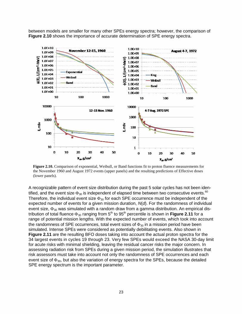
23

between models are smaller for many other SPEs energy spectra; however, the comparison of Figure 2.10 shows the importance of accurate determination of SPE energy spectra.

A recognizable pattern of event size distribution during the past 5 solar cycles has not been iden-

tified, and the event size 30 is independent of elapsed time between two consecutive events.60

Therefore, the individual event size 30 for each SPE occurrence must be independent of the expected number of events for a given mission duration, N(d). For the randomness of individual

event size, 30 was simulated with a random draw from a gamma distribution. An empirical dis-

tribution of total fluence 30 ranging from 5th to 95th percentile is shown in Figure 2.11 for a range of potential mission lengths. With the expected number of events, which took into account

the randomness of SPE occurrences, total event sizes of 30 in a mission period have been simulated. Intense SPEs were considered as potentially debilitating events. Also shown in Figure 2.11 are the resulting BFO doses taking into account the actual proton spectra for the 34 largest events in cycles 19 through 23. Very few SPEs would exceed the NASA 30-day limit for acute risks with minimal shielding, leaving the residual cancer risks the major concern. In assessing radiation risk from SPEs during a given mission period, the simulation illustrates that risk assessors must take into account not only the randomness of SPE occurrences and each

event size of 30, but also the variation of energy spectra for the SPEs, because the detailed SPE energy spectrum is the important parameter.

Figure 2.10. Comparison of exponential, Weibull, or Band functions fit to proton fluence measurements for

the November 1960 and August 1972 events (upper panels) and the resulting predictions of Effective doses

(lower panels).

24

2.3 Physics Model Description of Organ Exposures Descriptions of the fluence for each particle type and energy at each tissue of interest must be characterized before risk projections can be made. Fortunately, radiation transport codes validated by extensive measurements have been combined with accurate descriptions of the space environment to make accurate predictions of exposures to sensitive tissue sites behind spacecraft shielding or on planetary surfaces. Radiation transport codes were studied extensively in the past, and currently there are only minor scientific questions that lead to errors in the assess-ment of space radiation environments. Boltzmann equation solvers or Monte-Carlo algorithms can be used for this purpose when they are combined with models of the space environment as well as spacecraft and organ shielding. Monte-Carlo codes require long computational times to describe spacecraft with thousands of parts. Complex geometries are typically handled with simplifications in the representation by combining parts and material composition, thus negating any advantages compared to the one-dimensional transport methods that could be found by treatment of detailed three-dimensional effects. Boltzmann equation solvers such as the HZETRN code69 are able to use ray-tracing techniques to consider a very detailed geometry in a one-dimensional approach that is adequate for fast ions, especially for the omnidirectional radiation sources in space. The relative contribution from low-energy charged ions that deviate from the straight-ahead approximation can be solved by quadratures, leaving only the angular deflections of neutrons and intermediate energy light ions with sufficient energy to produce nuclear reactions to be addressed when considering a deviation from one-dimensional transport. However, their relative contribution to a GCR transport problem may be small, reducing the significance of any errors due to a one-dimensional approach. The underlying physical processes described by transport codes are atomic energy loss, straggling, and nuclear collisions. For describing atomic processes, the LET (stopping power), range, and energy straggling parameters are known to ±5% accuracy.33 A wide range of nuclear interactions occurs in GCR transport leading to a diverse range of secondary particles as described in Table 2.5.5,70 The nuclear cross sections needed for space radiation transport include nuclear

Figure 2.11. (Left panel) Simulated distribution of integral proton fluence above 30 MeV, 30 as a function of

increasing mission length. (Right panel) The blood-forming organ (BFO) dose behind 5 g/cm2 aluminum shields

from the 34 largest SPEs in the Space Age ranked by 30-MeV proton integral fluence, F>30 MeV calculated by the

BRYNTRN code.60

The black circles show the doses from each of the 34 events. The error bands show the 90%

CLs due to the variability of the proton energy spectra of the 34 events. The red dashed line shows the NASA 30-

day dose limit for the BFO.

1.E+04

1.E+05

1.E+06

1.E+07

1.E+08

1.E+09

1.E+10

1.E+11

0 50 100 150 200 250 300 350 400

Mission period, d

30, p

roto

ns c

m-2

95 percentile 90 percentile 75 percentile

Median with 5th & 95th percentile 25 percentile 10 percentile

5 percentile Max

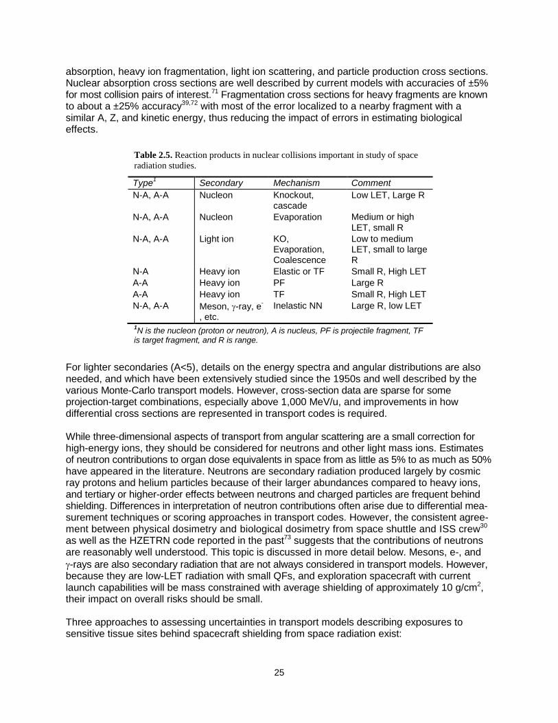
25

absorption, heavy ion fragmentation, light ion scattering, and particle production cross sections. Nuclear absorption cross sections are well described by current models with accuracies of ±5% for most collision pairs of interest.71 Fragmentation cross sections for heavy fragments are known to about a ±25% accuracy39,72 with most of the error localized to a nearby fragment with a similar A, Z, and kinetic energy, thus reducing the impact of errors in estimating biological effects.

For lighter secondaries (A<5), details on the energy spectra and angular distributions are also needed, and which have been extensively studied since the 1950s and well described by the various Monte-Carlo transport models. However, cross-section data are sparse for some projection-target combinations, especially above 1,000 MeV/u, and improvements in how differential cross sections are represented in transport codes is required. While three-dimensional aspects of transport from angular scattering are a small correction for high-energy ions, they should be considered for neutrons and other light mass ions. Estimates of neutron contributions to organ dose equivalents in space from as little as 5% to as much as 50% have appeared in the literature. Neutrons are secondary radiation produced largely by cosmic ray protons and helium particles because of their larger abundances compared to heavy ions, and tertiary or higher-order effects between neutrons and charged particles are frequent behind shielding. Differences in interpretation of neutron contributions often arise due to differential mea-surement techniques or scoring approaches in transport codes. However, the consistent agree-ment between physical dosimetry and biological dosimetry from space shuttle and ISS crew30 as well as the HZETRN code reported in the past73 suggests that the contributions of neutrons are reasonably well understood. This topic is discussed in more detail below. Mesons, e-, and

-rays are also secondary radiation that are not always considered in transport models. However, because they are low-LET radiation with small QFs, and exploration spacecraft with current launch capabilities will be mass constrained with average shielding of approximately 10 g/cm2, their impact on overall risks should be small. Three approaches to assessing uncertainties in transport models describing exposures to sensitive tissue sites behind spacecraft shielding from space radiation exist:

Table 2.5. Reaction products in nuclear collisions important in study of space

radiation studies.

Type1 Secondary Mechanism Comment

N-A, A-A Nucleon Knockout, cascade

Low LET, Large R

N-A, A-A Nucleon Evaporation Medium or high LET, small R

N-A, A-A Light ion KO, Evaporation, Coalescence

Low to medium LET, small to large R

N-A Heavy ion Elastic or TF Small R, High LET

A-A Heavy ion PF Large R

A-A Heavy ion TF Small R, High LET

N-A, A-A Meson, -ray, e-

, etc.

Inelastic NN Large R, low LET

1N is the nucleon (proton or neutron), A is nucleus, PF is projectile fragment, TF

is target fragment, and R is range.

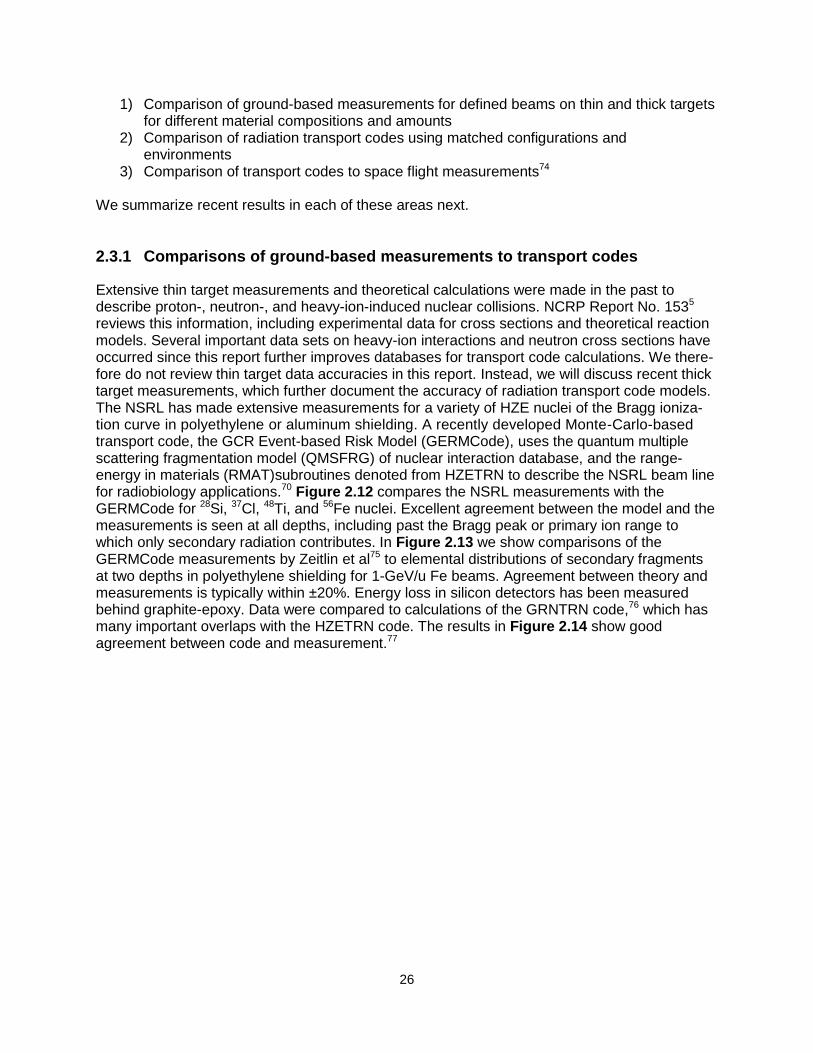
26

1) Comparison of ground-based measurements for defined beams on thin and thick targets for different material compositions and amounts

2) Comparison of radiation transport codes using matched configurations and environments

3) Comparison of transport codes to space flight measurements74 We summarize recent results in each of these areas next.

2.3.1 Comparisons of ground-based measurements to transport codes

Extensive thin target measurements and theoretical calculations were made in the past to describe proton-, neutron-, and heavy-ion-induced nuclear collisions. NCRP Report No. 1535 reviews this information, including experimental data for cross sections and theoretical reaction models. Several important data sets on heavy-ion interactions and neutron cross sections have occurred since this report further improves databases for transport code calculations. We there-fore do not review thin target data accuracies in this report. Instead, we will discuss recent thick target measurements, which further document the accuracy of radiation transport code models. The NSRL has made extensive measurements for a variety of HZE nuclei of the Bragg ioniza-tion curve in polyethylene or aluminum shielding. A recently developed Monte-Carlo-based transport code, the GCR Event-based Risk Model (GERMCode), uses the quantum multiple scattering fragmentation model (QMSFRG) of nuclear interaction database, and the range-energy in materials (RMAT)subroutines denoted from HZETRN to describe the NSRL beam line for radiobiology applications.70 Figure 2.12 compares the NSRL measurements with the GERMCode for 28Si, 37Cl, 48Ti, and 56Fe nuclei. Excellent agreement between the model and the measurements is seen at all depths, including past the Bragg peak or primary ion range to which only secondary radiation contributes. In Figure 2.13 we show comparisons of the GERMCode measurements by Zeitlin et al75 to elemental distributions of secondary fragments at two depths in polyethylene shielding for 1-GeV/u Fe beams. Agreement between theory and measurements is typically within ±20%. Energy loss in silicon detectors has been measured behind graphite-epoxy. Data were compared to calculations of the GRNTRN code,76 which has many important overlaps with the HZETRN code. The results in Figure 2.14 show good agreement between code and measurement.77

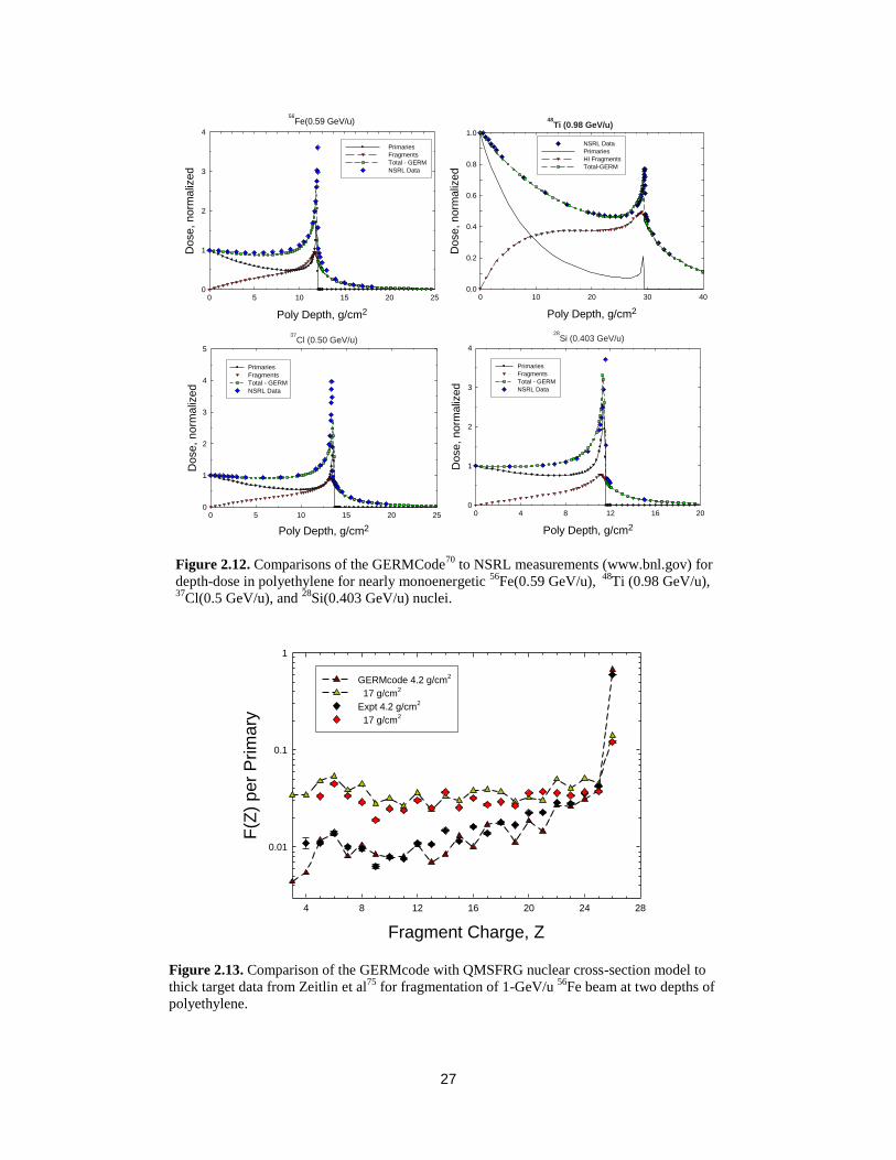
27

Figure 2.13. Comparison of the GERMcode with QMSFRG nuclear cross-section model to

thick target data from Zeitlin et al75

for fragmentation of 1-GeV/u 56

Fe beam at two depths of

polyethylene.

Fragment Charge, Z

4 8 12 16 20 24 28

F(Z

) p

er

Prim

ary

0.01

0.1

1

GERMcode 4.2 g/cm2

17 g/cm2

Expt 4.2 g/cm2

17 g/cm2

Figure 2.12. Comparisons of the GERMCode70

to NSRL measurements (www.bnl.gov) for

depth-dose in polyethylene for nearly monoenergetic 56

Fe(0.59 GeV/u), 48

Ti (0.98 GeV/u), 37

Cl(0.5 GeV/u), and 28

Si(0.403 GeV/u) nuclei.

48Ti (0.98 GeV/u)

Poly Depth, g/cm2

0 10 20 30 40

Dose,

norm

aliz

ed

0.0

0.2

0.4

0.6

0.8

1.0

NSRL Data

Primaries

HI Fragments

Total-GERM

56Fe(0.59 GeV/u)

Poly Depth, g/cm2

0 5 10 15 20 25

Dose,

norm

aliz

ed

0

1

2

3

4

Primaries

Fragments

Total - GERM

NSRL Data

28Si (0.403 GeV/u)

Poly Depth, g/cm2

0 4 8 12 16 20

Dose,

norm

aliz

ed

0

1

2

3

4

Primaries

Fragments

Total - GERM

NSRL Data

37Cl (0.50 GeV/u)

Poly Depth, g/cm2

0 5 10 15 20 25

Dose, norm

aliz

ed

0

1

2

3

4

5

Primaries

Fragments

Total - GERM

NSRL Data

28

2.3.2 Comparisons of transport codes

Recently, Wilson (private communications, 2009) organized comparisons of the HZETRN code to several Monte-Carlo codes for well-defined shielding configurations and identical source energy spectra for GCR and SPEs. The Monte-Carlo codes considered were HETC-HEDS,78 FLUKA,79 and PHITS.80 These results, as summarized in both Figure 2.15 and Figure 2.16, are in very good agreement for depth-dose, depth-dose-equivalent, and light-particle energy spectra. Some of the comparisons on organ doses did not consider all of the contributions from target fragments that introduce several differences between the code comparisons. These comparisons show that overall agreement between transport code predictions, when compared with identical source spectra and shielding configuration, is quite high. A possible

minor discrepancy is the mesons, electrons, and -rays that may contribute 5% to 10% of the absorbed dose from GCR behind ISS levels of shielding, and 1% to 3% of the dose equivalent because of their small QFs or RBEs compared to HZE nuclei, or to stopping protons and helium nuclei. These processes have not been fully integrated into all versions of the various existing codes, and should be considered for deep-shielding risk assessment (>50 g/cm2). Further considerations on pions are described below.

Figure 2.14. Comparisons of GRNTRN code to measurements for the summed

energy loss in a silicon detector from fragments of a 1053-MeV/u 56

Fe beam behind

10 g/cm2 graphite-epoxy (51%/49%) (reproduced from Walker et al).

77

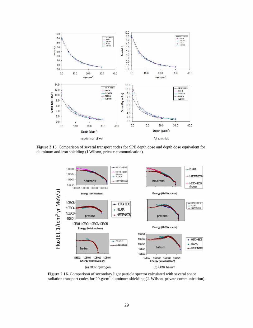
29

Figure 2.16. Comparison of secondary light particle spectra calculated with several space

radiation transport codes for 20-g/cm2 aluminum shielding (J. Wilson, private communication).

Figure 2.15. Comparison of several transport codes for SPE depth dose and depth dose equivalent for

aluminum and iron shielding (J Wilson, private communication).

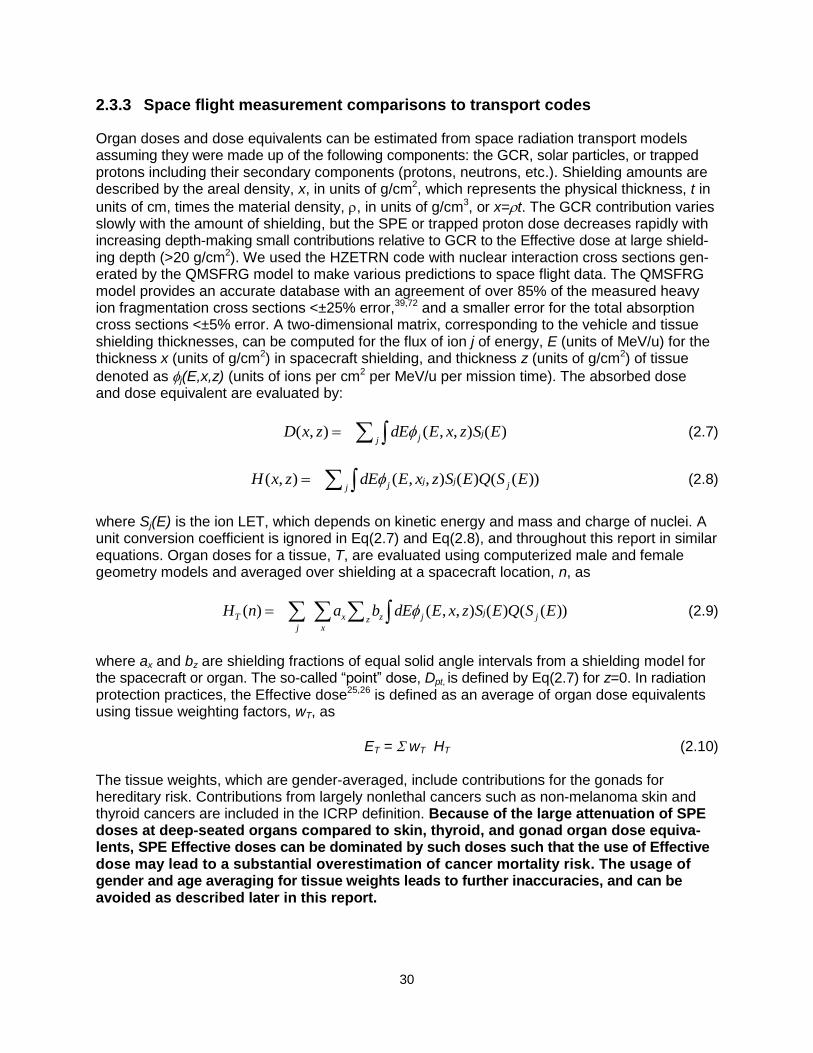
30

2.3.3 Space flight measurement comparisons to transport codes

Organ doses and dose equivalents can be estimated from space radiation transport models assuming they were made up of the following components: the GCR, solar particles, or trapped protons including their secondary components (protons, neutrons, etc.). Shielding amounts are described by the areal density, x, in units of g/cm2, which represents the physical thickness, t in

units of cm, times the material density, , in units of g/cm3, or x=t. The GCR contribution varies slowly with the amount of shielding, but the SPE or trapped proton dose decreases rapidly with increasing depth-making small contributions relative to GCR to the Effective dose at large shield-ing depth (>20 g/cm2). We used the HZETRN code with nuclear interaction cross sections gen-erated by the QMSFRG model to make various predictions to space flight data. The QMSFRG model provides an accurate database with an agreement of over 85% of the measured heavy ion fragmentation cross sections <±25% error,39,72 and a smaller error for the total absorption cross sections <±5% error. A two-dimensional matrix, corresponding to the vehicle and tissue shielding thicknesses, can be computed for the flux of ion j of energy, E (units of MeV/u) for the thickness x (units of g/cm2) in spacecraft shielding, and thickness z (units of g/cm2) of tissue

denoted as j(E,x,z) (units of ions per cm2 per MeV/u per mission time). The absorbed dose and dose equivalent are evaluated by:

( , ) ( , , ) ( )jjjD x z dE E x z S E (2.7)

( , ) ( , , ) ( ) ( ( ))j jj jjH x z dE E x z S E Q S E (2.8)

where Sj(E) is the ion LET, which depends on kinetic energy and mass and charge of nuclei. A unit conversion coefficient is ignored in Eq(2.7) and Eq(2.8), and throughout this report in similar equations. Organ doses for a tissue, T, are evaluated using computerized male and female geometry models and averaged over shielding at a spacecraft location, n, as

( ) ( , , ) ( ) ( ( ))jT x z j jzj x

H n a b dE E x z S E Q S E (2.9)

where ax and bz are shielding fractions of equal solid angle intervals from a shielding model for the spacecraft or organ. The so-called ―point‖ dose, Dpt, is defined by Eq(2.7) for z=0. In radiation protection practices, the Effective dose25,26 is defined as an average of organ dose equivalents using tissue weighting factors, wT, as

ET = wT HT (2.10) The tissue weights, which are gender-averaged, include contributions for the gonads for hereditary risk. Contributions from largely nonlethal cancers such as non-melanoma skin and thyroid cancers are included in the ICRP definition. Because of the large attenuation of SPE doses at deep-seated organs compared to skin, thyroid, and gonad organ dose equiva-lents, SPE Effective doses can be dominated by such doses such that the use of Effective dose may lead to a substantial overestimation of cancer mortality risk. The usage of gender and age averaging for tissue weights leads to further inaccuracies, and can be avoided as described later in this report.

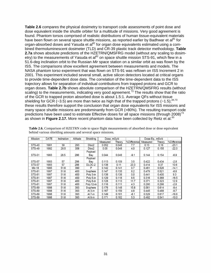
31

Table 2.6 compares the physical dosimetry to transport code assessments of point dose and dose equivalent inside the shuttle orbiter for a multitude of missions. Very good agreement is found. Phantom torsos comprised of realistic distributions of human tissue-equivalent materials have been flown on several space shuttle missions, as reported earlier by Badhwar et al81 for organ-absorbed doses and Yasuda et al82 for organ dose equivalents estimated using a com-bined thermoluminescent dosimeter (TLD) and CR-39 plastic track detector methodology. Table 2.7a shows absolute predictions of the HZETRN/QMSFRG model (without any scaling to dosim-etry) to the measurements of Yasuda et al82 on space shuttle mission STS-91, which flew in a 51.6-deg inclination orbit to the Russian Mir space station on a similar orbit as was flown by the ISS. The comparisons show excellent agreement between measurements and models. The NASA phantom torso experiment that was flown on STS-91 was reflown on ISS Increment 2 in 2001. This experiment included several small, active silicon detectors located at critical organs to provide time-dependent dose data. The correlation of the time-dependent data to the ISS trajectory allows for separation of individual contributions from trapped protons and GCR to organ doses. Table 2.7b shows absolute comparison of the HZETRN/QMSFRG results (without scaling) to the measurements, indicating very good agreement.73 The results show that the ratio of the GCR to trapped proton absorbed dose is about 1.5:1. Average QFs without tissue shielding for GCR (~3.5) are more than twice as high that of the trapped protons (~1.5);34,73 these results therefore support the conclusion that organ dose equivalents for ISS missions and many space shuttle missions are predominantly from GCR (>80%). The resulting transport code predictions have been used to estimate Effective doses for all space missions (through 2008)73 as shown in Figure 2.17. More recent phantom data have been collected by Reitz et al.83

Table 2.6. Comparison of HZETRN code to space flight measurements of absorbed dose or dose equivalent

behind various shielding amounts and several space missions.

32

Figure 2.17. Summary of mission badge dose, Effective dose, and population average biological dose equivalent

for astronauts on all NASA space missions, including Mercury, Gemini, Apollo, Skylab, Apollo-Soyuz, space

shuttle, NASA-Mir and ISS missions.73

Astronaut, i

0 100 200 300 400 500 600 700 800

Mis

sio

n D

ose

0.1

1

10

100

1000

Badge Dose, mGy

Effective Dose, mSv

Biodosimetry, mGy-EqSkylab, Mir and ISS

Mercury

Apollo and Shuttle

Gemini

Hubble Missions

Table 2.7.b. Comparison of small active dosimetry data from ISS Increment 2 phantom torso (for July-August 2001) to

predictions from the HZETRN/QMSFRG model.73

Organ Trapped, mGy/d GCR, mGy/d Total Dose, mGy/d Difference

(%) Expt. Model Expt. Model Expt. Model

Brain 0.051 0.066 0.076 0.077 0.127 0.143 13.3 Thyroid 0.062 0.072 0.074 0.077 0.136 0.148 9.4 Heart 0.054 0.061 0.075 0.076 0.129 0.137 6.7 Stomach 0.050 0.057 0.076 0.077 0.126 0.133 5.5 Colon 0.055 0.056 0.073 0.076 0.128 0.131 2.5

Table 2.7.a. Comparison of measured organ dose equivalent for STS-91 mission by Yasuda et al.82

using

combined CR-39/TLD method to predictions from the HZETRN/QMSFRG space transport model.

Organ Dose Equivalent, mSv

Tissue Measured HZETRN/QMSFRG Difference (%) Skin 4.5 +0.05 4.7 4.4 Thyroid 4.0 +0.21 4.0 0 Bone surface 5.2 +0.22 4.0 -23.1 Esophagus 3.4 +0.49 3.7 8.8 Lung 4.4 +0.76 3.8 -13.6 Stomach 4.3 +0.94 3.6 -16.3 Liver 4.0 +0.51 3.7 -7.5 Bone marrow 3.4 +0.40 3.9 14.7 Colon 3.6 +0.42 3.9 8.3 Bladder 3.6 +0.24 3.5 -2.8 Gonad 4.7 +0.71 3.9 -17.0 Chest 4.5 +0.11 4.5 0 Remainder 4.0 +0.57 4.0 0

Effective dose 4.1 +0.22 3.9 -4.9

33

Energy spectra for light particles measured with particle hodoscopes are in good agreement with the HZETRN code as shown in Figure 2.18.84 Measurements of heavy-ion spectra require a large area detector, and very few such measurements have been made in human-rated vehi-cles because of mass requirements. Other space flight measurements of LET or microdosimetry measurements of lineal energy spectra using tissue-equivalent proportional counters (TEPCs) have also been shown to be in good agreement with transport codes.85,86 Agreement is obviously improved when models of detector response are used to make such comparisons. Corrections of measurements often involve model-dependent assumptions, such as the conversion from silicon to tissue-equivalent LET spectra in which the conversion factor is dependent on energy and charge number. Also, the combined TLD plus CR-39 method for estimating dose equivalent82 involves corrections on the high-LET sensitivity of TLDs and the low-LET sensitivity of CR-39. Comparisons of codes to TEPCs data require the conversion of energy and charge spectra into lineal energy spectra, which differ substantially from LET spectra. Comparisons of models to measurements of neutron spectra on the Russian Mir space station were in good agreement (Fig. 2.19). The major fraction of the neutron dose is for energies >10 MeV, with a smaller fraction <10 MeV. At these higher energies, secondary recoil nuclei produced by neutrons are very similar in Z and E to those produced by high-energy protons. Therefore, at equal fluence, high-energy protons are more biologically effective than neutrons of the same energy because of the charge carried by protons.

Figure 2.18. Comparisons of proton (Panel A) and Deuteron (Panel B) energy distributions from

GCR on the STS-48 mission to HZETRN results.84

The dash line and solid line are without or with

cluster knockouts, respectively.

34

2.3.4 Predictions for exploration missions

We show the organ doses for GCR at solar minimum and the 1972 SPE for depths of 5 and 20 g/cm2 diameter in aluminum spheres In Table 2.8. The 1972 solar event is represented by the protons fluence spectrum derived by King.65 SPE spectra are greatly attenuated with shielding and show important variations in doses between tissue types, whereas GCR produces only a modest variation between organs at both depths. The point doses shown correspond to the dose without tissue shielding. Values of point doses are well above organ doses for SPEs and similar to organ doses for GCR. Doses to the skin can be several times higher than those of the internal organs for SPEs.88 Average skin doses do not properly describe the risk to specific skin loci, which are highly variable. Annual GCR Effective doses are calculated in Figure 2.20 for various charge groups inside a spacecraft of 50 g/cm2 aluminum from GCR at solar minimum in interplanetary space (blue bars). These heavy nuclei are a concern for radiation risks because they have the highest biological effectiveness and leave columns of damage at the molecular level as they traverse a biological system, and because a plausible mitigation measure by shielding is impossible due to the high penetration power of energetic particles of GCR.

Figure 2.19. Comparisons of transport codes to ISS neutron spectra measurements.87

35

Table 2.8. Organ doses for males inside aluminum shields for 1972 SPE and GCR at solar minimum.

(a) 5-g/cm2 aluminum

Organ/tissue

August 1972 SPE Annual GCR at solar minimum

D

mGy

G

mGy-Eq

H

mSv

D

mGy

G

mGy-Eq

H

mSv

Avg. Skin 2692.3 4052.1 4259.7 198.8 375.8 832.3

Avg. BFO 306.9 462.5 442.1 185.7 337.2 614.0

Stomach 112.3 169.6 168.0 182.2 324.4 547.6

Colon 251.4 379.0 363.8 185.6 336.4 606.2

Liver 174.1 262.7 255.0 183.1 327.9 566.6

Lung 205.6 310.1 299.4 184.5 332.9 590.9

Esophagus 195.4 294.8 285.0 184.0 331.3 584.4

Bladder 118.7 179.2 176.8 181.6 322.5 540.8

Thyroid 333.2 502.1 479.0 186.8 341.1 632.7

Chest/Breast 1615.9 2430.6 2323.9 194.1 365.6 770.2

Gonads/Ovarian 748.1 1125.7 1072.2 186.5 339.7 640.9

Front brain 571.7 860.9 816.4 190.6 354.4 696.9

Mid brain 279.6 421.5 403.9 187.7 344.1 640.2

Rear brain 557.5 839.6 796.2 190.5 354.0 695.2

Lens 1959.0 2946.2 2829.4 196.2 372.4 806.3

Gallbladder 118.7 179.2 176.8 181.6 322.5 540.8

Remainder 406.3 611.9 585.9 186.1 338.2 619.5

Point Dose 5389.0 8125.0 8663.0 218.2 434.4 1140.7

E, mSv wT (ICRP 1991)

612.3

611.1

wT (ICRP 2007)

676.2

620.7

(b) 20-g/cm2 aluminum

Organ/tissue

August 1972 SPE Annual GCR at solar minimum

D

mGy

G

mGy-Eq

H

mSv

D

mGy

G

mGy-Eq

H

mSv

Avg. Skin 87.8 132.8 144.0 193.5 342.3 599.8

Avg. BFO 23.4 35.7 42.9 182.0 314.9 494.2

Stomach 12.1 18.6 25.5 179.1 306.4 465.5

Colon 21.0 32.1 39.4 181.9 314.6 491.3

Liver 15.6 23.8 30.7 179.8 308.6 473.6

Lung 18.3 28.0 35.2 180.9 312.0 484.4

Esophagus 17.5 26.8 34.0 180.5 310.9 481.4

Bladder 12.0 18.4 25.0 178.6 305.0 462.2

Thyroid 25.7 39.1 46.5 182.9 317.5 502.5

Chest/Breast 67.2 101.9 107.0 189.0 333.8 558.7

Gonads/Ovarian 37.5 57.0 62.5 182.5 316.1 503.3

Front brain 37.6 57.1 64.8 186.1 326.6 530.5

Mid brain 24.0 36.7 44.8 183.7 319.8 506.9

Rear brain 37.0 56.4 64.0 186.0 326.4 529.8

Lens 76.7 116.1 120.9 190.8 338.4 574.0

Heart* 18.3 28.0 35.2 180.9 312.0 484.4

Gallbladder 12.0 18.4 25.0 178.6 305.0 462.2

Remainder 26.0 39.6 46.5 182.3 315.6 496.3

Point Dose 164.7 248.9 267.8 210.7 384.3 751.4

E, mSv wT (ICRP 1991)

45.83

492.48

wT (ICRP 2007)

48.45

496.74

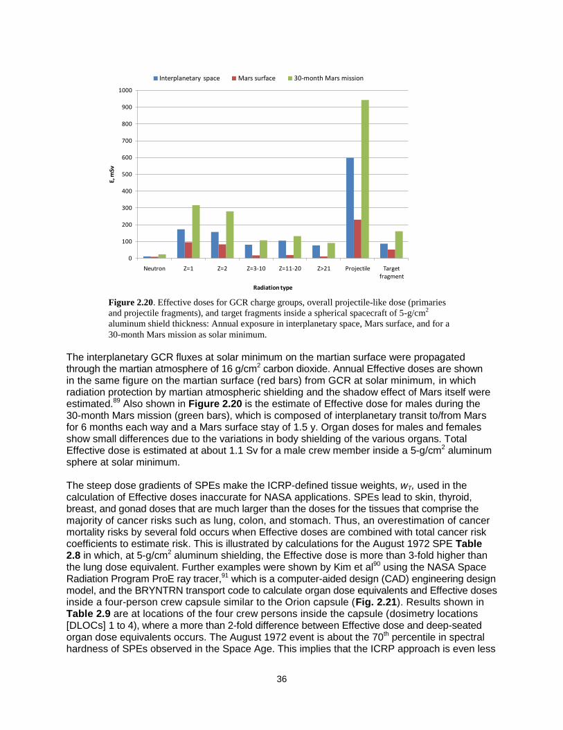
36

The interplanetary GCR fluxes at solar minimum on the martian surface were propagated through the martian atmosphere of 16 g/cm2 carbon dioxide. Annual Effective doses are shown in the same figure on the martian surface (red bars) from GCR at solar minimum, in which radiation protection by martian atmospheric shielding and the shadow effect of Mars itself were estimated.89 Also shown in Figure 2.20 is the estimate of Effective dose for males during the 30-month Mars mission (green bars), which is composed of interplanetary transit to/from Mars for 6 months each way and a Mars surface stay of 1.5 y. Organ doses for males and females show small differences due to the variations in body shielding of the various organs. Total Effective dose is estimated at about 1.1 Sv for a male crew member inside a 5-g/cm2 aluminum sphere at solar minimum. The steep dose gradients of SPEs make the ICRP-defined tissue weights, wT, used in the calculation of Effective doses inaccurate for NASA applications. SPEs lead to skin, thyroid, breast, and gonad doses that are much larger than the doses for the tissues that comprise the majority of cancer risks such as lung, colon, and stomach. Thus, an overestimation of cancer mortality risks by several fold occurs when Effective doses are combined with total cancer risk coefficients to estimate risk. This is illustrated by calculations for the August 1972 SPE Table 2.8 in which, at 5-g/cm2 aluminum shielding, the Effective dose is more than 3-fold higher than the lung dose equivalent. Further examples were shown by Kim et al90 using the NASA Space Radiation Program ProE ray tracer,91 which is a computer-aided design (CAD) engineering design model, and the BRYNTRN transport code to calculate organ dose equivalents and Effective doses inside a four-person crew capsule similar to the Orion capsule (Fig. 2.21). Results shown in Table 2.9 are at locations of the four crew persons inside the capsule (dosimetry locations [DLOCs] 1 to 4), where a more than 2-fold difference between Effective dose and deep-seated organ dose equivalents occurs. The August 1972 event is about the 70th percentile in spectral hardness of SPEs observed in the Space Age. This implies that the ICRP approach is even less

Figure 2.20. Effective doses for GCR charge groups, overall projectile-like dose (primaries

and projectile fragments), and target fragments inside a spherical spacecraft of 5-g/cm2

aluminum shield thickness: Annual exposure in interplanetary space, Mars surface, and for a

30-month Mars mission as solar minimum.

0

100

200

300

400

500

600

700

800

900

1000

Neutron Z=1 Z=2 Z=3-10 Z=11-20 Z>21 Projectile Target fragment

E, m

Sv

Radiation type

Interplanetary space Mars surface 30-month Mars mission

37

accurate for fatal cancer risk estimates for most other SPEs compared to results for the 1972 event because the dose gradient is larger for the many ―softer‖ SPE spectra.

Table 2.9. August 1972 SPE organ dose quantities for males using the fully automated ProE

structural distribution model LTV, the computerized anatomical man model (CAMERA), and

the BRYNTRN codes. The King spectra for the SPE is used. Calculations are at the location of

each crew member in the LTV.

Organ Dose Equivalent, mSv

DLOC1 DLOC2 DLOC3 DLOC4

Al-Eq xavg, g/cm2 15.18 15.08 15.85 15.33

CAM

organ

dose

Avg. skin 1266 1211 1041 1086

Eye 868 844 736 771

Avg. BFO 169 168 152 159

Stomach 73.8 73.7 67.7 70.3

Colon 144 144 130 136

Liver 104 103 94.1 98.0

Lung 122 121 110 115

Esophagus 116 116 105 110

Bladder 75.4 75.3 69.0 717

Thyroid 184 183 166 173

Chest 722 706 619 648

Gonads 353 347 308 322

Front brain 295 293 263 275

Mid brain 162 162 147 153

Rear brain 289 287 258 270

Effective Dose, mSv 213 210 188 196

Point Dose Eq., mSv 2557 2427 2079 2168

Figure 2.21. Visualization of detailed directional dose assessment at a dosimetry location (DLOC1) inside

a conceptual spacecraft representative of a lunar transfer vehicle (LTV). The spacecraft is shown in a

translucent view to reveal the exact dosimetry location (left), and the same directional dose assessment is

shown separately in the large view (right).

38

2.4 Dose Contributions from Pions and Pion Decays Pions are produced in nuclear reactions of GCR particles with shielding and tissue at energies above a few hundred MeV/u. The number of pions produced increases with kinetic energy of the GCR particle with multi-pion production processes occurring above about 500 MeV/u. The pion production cross section increases with mass number with an approximate 2/3 power; therefore, most pions are produced in GCR transport by protons, helium, and secondary neutrons because of their much higher abundances compared to HZE particles. Pion production is not important for SPEs and trapped protons because of their primary proton energies. Pions and their decay products can make an important contribution to GCR dose equivalent as shielding thickness increases beyond about 50 g/cm2 for aluminum and similar depth for other materials.

The three charge components of pions (+, -, 0) have different characteristics in radiation

transport in shielding and tissue. Neutral pions decay almost instantaneously into -rays of very

high energy. High energy -rays produce electron-positron pairs and photo-nuclear reactions. The charged pions decay into muons and neutrinos. The two pion charge states have similar transport characteristics above about 100 MeV with similar LET and nuclear production cross

sections. They differ at lower energy because the - can cause nuclear annihilation if it slows down and is captured by an atomic nucleus. Several transport codes have made predictions of the absorbed doses from pions and electromagnetic decays in GCR transport, including MCNPX,232 HZETRN,233 PHITS,234 FLUKA (B. Reddell, private communication). These estimates are summarized in Table 2.10. Differences between the codes are likely due to

differences in cross section models, and in the methods used to transport the higher energy -rays.

Table 2.10. Percentage of total GCR absorbed dose contributions from combined doses of pions, muons, electrons

and photons behind aluminum shielding estimated using several transport code models.232-234

Percentage Dose

equivalent contributions are about 3 times smaller occur because the average QF from pions and related particles is

much smaller compared to HZE particles and secondary neutrons.

%-Contributions to Total Absorbed Dose

Depth in Al, g/cm2 FLUKA MCNPX HZETRN (ISS) PHITS-ISS

5 - 5% 2% (2%)

10 15.3% 3% (5%)

20 17.7% 9% 6% (8%)

40 22.3% 13% (17%)

60 19% (25%)

80 31% (39%)

100 38% (47%)

~20 at skin (ISS) 13.5%

~20 at BFO (ISS) 6.2%

5 + 10 cm water 9%

20 + 10 cm water 13%

5 + 20 cm water 13%

20 + 20 cm water 16%

5 + 30 cm water 15%

20 + 30 cm water 18%

39

An empirical representation of the average dose contribution versus depth of shielding material, x, can be made as a fraction of the total GCR dose without pions and EM decays based on an average over the various transport code results for aluminum scaled to other materials using the average target mass number of the shielding:

)11.2()(4/3

1 xDxcD GCRpion

Where c1=0.011 [0.2+0.8(ATave/27)0.667], and ATave is the average target mass of the shielding material. For the QF of the average pion and EM decay dose, we estimate a value of 1.2 to account for target fragments from pion interactions, which have not been evaluated. Eq(2.10) is estimated to be accurate to within about +40%. Pions and their EM decays products makes a small contribution to the REID for shielding of areal density less than about 50 g/cm2, and more significant contributions at larger depths. Other dose or REID contributions from particle production processes, including that of kaons and anti-protons, should be smaller compared to pions. The radiobiology of Z=1 particles such as pions and muons of high energy and of photons above 5 MeV has not been well studied. Based on the track structure of these particles,

which is dominated by high energy -rays, we expect the RBE for most endpoints to be small (≤1) after the nuclear recoil components are accounted for.

Figure 2.22 compares the older BO96 model used in the HZETRN code at NASA for many years with the latest BO11 model. A detailed comparison of the BO96 model for protons and helium to balloon and satellite date for GCR suggests the model over-represented these particles. However, use of the BO11 model with the added dose contributions from pions and their decay products agrees very well with the BO96 environmental model without the doses from pions and decays products.

Figure 2.22. Annual GCR dose for 20 g/cm2 aluminum shielding for BO96 model and BO11 model

with or without dose contributions from pions and EM decays (photons, muons, and electrons).

Year

1996 1998 2000 2002 2004 2006 2008 2010 2012 2014

GC

R D

ose,

mG

y/y

r

0

50

100

150

200

250

BO96

BO11

BO11 with Pions/EM

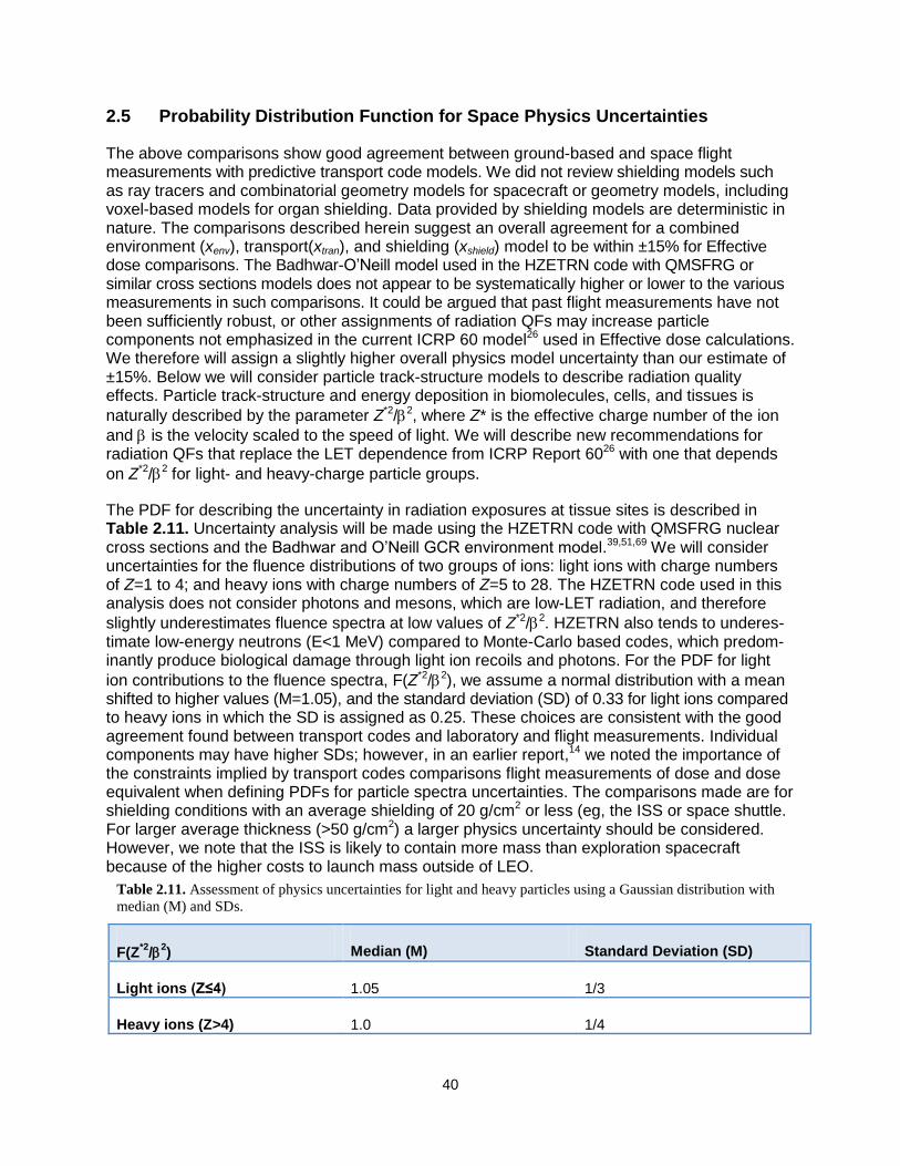
40

2.5 Probability Distribution Function for Space Physics Uncertainties

The above comparisons show good agreement between ground-based and space flight measurements with predictive transport code models. We did not review shielding models such as ray tracers and combinatorial geometry models for spacecraft or geometry models, including voxel-based models for organ shielding. Data provided by shielding models are deterministic in nature. The comparisons described herein suggest an overall agreement for a combined environment (xenv), transport(xtran), and shielding (xshield) model to be within ±15% for Effective dose comparisons. The Badhwar-O’Neill model used in the HZETRN code with QMSFRG or similar cross sections models does not appear to be systematically higher or lower to the various measurements in such comparisons. It could be argued that past flight measurements have not been sufficiently robust, or other assignments of radiation QFs may increase particle components not emphasized in the current ICRP 60 model26 used in Effective dose calculations. We therefore will assign a slightly higher overall physics model uncertainty than our estimate of ±15%. Below we will consider particle track-structure models to describe radiation quality effects. Particle track-structure and energy deposition in biomolecules, cells, and tissues is

naturally described by the parameter Z*2/2, where Z* is the effective charge number of the ion

and is the velocity scaled to the speed of light. We will describe new recommendations for radiation QFs that replace the LET dependence from ICRP Report 6026 with one that depends

on Z*2/2 for light- and heavy-charge particle groups.

The PDF for describing the uncertainty in radiation exposures at tissue sites is described in Table 2.11. Uncertainty analysis will be made using the HZETRN code with QMSFRG nuclear cross sections and the Badhwar and O’Neill GCR environment model.39,51,69 We will consider uncertainties for the fluence distributions of two groups of ions: light ions with charge numbers of Z=1 to 4; and heavy ions with charge numbers of Z=5 to 28. The HZETRN code used in this analysis does not consider photons and mesons, which are low-LET radiation, and therefore

slightly underestimates fluence spectra at low values of Z*2/2. HZETRN also tends to underes-timate low-energy neutrons (E<1 MeV) compared to Monte-Carlo based codes, which predom-inantly produce biological damage through light ion recoils and photons. For the PDF for light

ion contributions to the fluence spectra, F(Z*2/2), we assume a normal distribution with a mean shifted to higher values (M=1.05), and the standard deviation (SD) of 0.33 for light ions compared to heavy ions in which the SD is assigned as 0.25. These choices are consistent with the good agreement found between transport codes and laboratory and flight measurements. Individual components may have higher SDs; however, in an earlier report,14 we noted the importance of the constraints implied by transport codes comparisons flight measurements of dose and dose equivalent when defining PDFs for particle spectra uncertainties. The comparisons made are for shielding conditions with an average shielding of 20 g/cm2 or less (eg, the ISS or space shuttle. For larger average thickness (>50 g/cm2) a larger physics uncertainty should be considered. However, we note that the ISS is likely to contain more mass than exploration spacecraft because of the higher costs to launch mass outside of LEO.

Table 2.11. Assessment of physics uncertainties for light and heavy particles using a Gaussian distribution with

median (M) and SDs.

F(Z*2

/2) Median (M) Standard Deviation (SD)

Light ions (Z≤4) 1.05 1/3

Heavy ions (Z>4) 1.0 1/4

41

2.6. Summary of Research Needs in Space Physics As noted by the NRC,226 the current space environment models, radiation transport codes, and shielding models are very accurate, and further research has likely reached the point of diminishing returns. Nevertheless, such models require continued updates and sustainability including ensuring adequate personnel at NASA are qualified to update the various models and computer codes. Specifically:

1. Continued updates of GCR models most importantly with regards to solar modulation. 2. For SPE models, the approach of Kim et al218 should be updated as the current and

future solar cycles progress and new SPEs occur. A probabilistic model of the time profiles of SPEs should be developed.

3. Cross sectional models should be updated as new data becomes available and updated transport codes checked against important new flight measurements.

4. The HZETRN codes began integrating pions and EM decays in 1997. This work should be completed and checked against other computer codes.

5. The radiobiology of pions and high energy photons, muons, and electrons (>1 MeV) could be considered in the future.

42

3. Cancer Risk Projections for Low-linear Energy Transfer Radiation

The current radiation cancer risk projection model used at NASA is based on NCRP Report No. 132;6 however, this has been updated by NASA (PELs, 2006) to use the solid cancer mortality analysis made in LSS [Life-span Study of the Japanese atomic-bomb survivors] Report 13.9 These methods form the basis by which to calculate the current dose limits used at NASA; ie, age- and gender-specific Effective dose to reach a probability of 3% for REID. In recent years, there have been important new analyses of human epidemiology data by the BEIR VII Commit-tee,16 UNSCEAR,17 Preston et al,92 National Cancer Institute (NCI),93 Little et al,10,94 Pawel et al,95 and others. Important changes since NCRP Report No. 132 include a reevaluation of the A-bomb survivor doses denoted as DS02.96 Longer follow-up studies of the exposed cohorts with the most recent incidence data from the LSS from the Radiation Effects Research Foundation (RERF) cover the years 1958 through 1998.92 Meta-analysis of different exposed cohorts for specific tissues such as breast and thyroid cancers has been reported. Application of new meth-odologies includes Bayesian analysis of dosimetry errors10 and EB methods for tissue-specific cancer risk uncertainties.95 New analyses of the DDREF were made by the BEIR VII and Jacobs et al97 from a meta-analysis of 12 published radiation worker studies. An important change advocated by the BEIR VII report is to estimate cancer mortality risks by the transfer of incidence rates in exposed cohorts to populations under study (eg, the U.S.), and then to estimate mortality risks using the ratio of host population cancer mortality and incidence rates. Previous recommendations from the NCRP used mortality-based risk transfer models.6 In this section, we will review the mathematical approaches to calculate low-LET cancer risks and compare recent fits to the most recent LSS data.

The instantaneous incidence rate of cancer, (t), is defined in terms of the probability distribution function, F(t), of the time to cancer occurrence. The survival function, S(t), is the probability of being cancer-free at age t (the interval [0,t]), and is given by 1-F(t). The probability density function, f(t), is then dF(t)/dt. The hazard rate is the instantaneous incidence rate as is given by

( )

( )1 ( )

f tt

F t

(3.1)

The cumulative hazard, (t), also known as the cumulative incidence rate, is

0

( ) ( )

t

t z dz (3.2)

The survival probability is related to the cumulative hazard function by

( ) exp[ ( )]S t t (3.3)

To model radiation risk along with radiation hazard rates, the age- and gender-specific survival probability (often represented by a life-table) must be described because of the role of competing causes of death. For multiplicative risk models (described below), the age- and gender-specific hazard rates for cancer incidence or mortality in the population under study also must be defined.

43

The instantaneous cancer rate (mortality or incidence) can be a function of dose, D, or dose-rate, Dr, gender, age at exposure, aE, attained age, a, or latency, which is the time after expo-sure, L=a-aE. These dependencies may vary for each cancer type that could be increased by

radiation exposure. Hazard rates for cancer incidence, I, and cancer mortality, M, can be modeled with similar approaches. The REID is calculated by folding the probability of surviving to time, t, which is represented as the survival function, S0(t), for the background population times into the probability for radiation cancer death at a previous time with the instantaneous radiation cancer mortality rate and then integrating over the remainder of a lifetime:

( , , )

0( , ) ( , , ) ( )

t

M EaE

E

dz z a D

E M E

a

REID a D dt a a D S t e

(3.4)

Similarly, the REIC incidence uses a radiation cancer incidence rate folded with the probability to survive to time, t, and integrated over the remainder of a lifetime:

( , , )

0( , ) ( , , ) ( )

t

M Ea

E

E

dz z a D

E I E

a

REIC a D dt a a D S t e

(3.5)

The BEIR VII report16 uses the quantity LAR instead of REID as the primary measure of risk. Others committees98 have used the quantity ELR. (Note: NCRP Report No. 132 discusses results in terms of ELR; however, the formula on page 127 of the report suggests that REID was calculated in the report.) The LAR and ELR risk measures have important deficiencies and are not used at NASA. The ELR ignores cancer deaths that would have occurred anyway in a population but are moved to an earlier time point due to radiation exposure. ELR, therefore, underestimates risks. The LAR ignores the radiation contribution to the survival probability in Eq(3.4) or Eq(3.5). It thus leads to an overestimation of risk, especially at high doses, and also can lead to errors in uncertainty analysis when large risk values are sampled in Monte-Carlo trials.

3.1 Cancer Mortality and Incidence Rates Radiation cancer incidence (or mortality) rates are most often modeled in the multiplicative risk model that is also denoted as the excess relative risk (ERR) model in which the radiation cancer rates are proportional to background cancer rates given by:

0( , , ) ( )[1 ( , , )]I E I Ea a D a ERR a a D (3.6)

where i0(a) is the age-specific (and tissue- and gender-specific) cancer rate from background cancers in the population under study. A second model is also used; this study, denoted as the excess additive risk (EAR) model, does not explicitly depend on the background cancer rates given by:

( , , ) ( , , )I E Ea a D EAR a a D (3.7)

Radiation cancer rates can be fitted to data on all cancers or various sub-categories including tissue-specific cancer rates. Overall cancer incidence data have lower statistical uncertainties

44

than overall mortality data because of higher counts. Projecting tissue-specific cancer incidence probabilities has higher statistical uncertainties due to lower counts compared to fitting grouped data such as all solid cancers and leukemias. However, projections based on tissue-specific in-cidence data offer many advantages, including the possibility to apply tissue-specific transfer models between populations, tissue-specific radiation quality, and dose-rate dependencies. Attributable risks calculations for estimating probability of causation on disease discovery are evaluated with tissue-specific incidence models.93 The astronaut informed-consent process is also improved if information on specific cancer types for both incidence and mortality risks is provided. More recently, an EB method has been shown to provide an improved representation of statistical errors in tissue-specific risks.95 A multiplicative risk model for projecting cancer mortality (REID) from tissue-specific cancer incidence uses identical ERR functions determined for incidence to project tissue-specific mor-tality using population cancer incidence rate to mortality rate scaling.16 Similarly, an additive risk model derived from incidence data can be used for mortality risk prediction by adjusting EAR functions derived from incidence data by the ratio of background mortality to incidence rates:16

0

0

( )( , , ) ( , , )

( )

MM E E

I

aa a D EAR a a D

a

(3.8)

Various advisory reports have used distinct approaches to arrive at assumptions on how to combine multiplicative and additive risk model estimates. A weighting of the multiplicative transfer

model, denoted as T, can be introduced. The additive transfer model weight is then given by 1-T. NCRP Report No. 132 recommended to use an arithmetic mean of the additive and multiplicative risk models for all solid cancers and the additive risk model for leukemia risk. Although the recent UNSCEAR report17 did not make a recommendation on risk transfer models, we note that its mul-tiplicative risk model provides the best fit to the LSS. The BEIR VII report uses geometric means

of the additive and multiplicative transfer models for most cancer types with a weight T of 0.7 including leukemia, but deviates for lung, breast, and thyroid cancer risk estimates. For lung

cancer, BEIR VII assigns a weight T of 0.3, favoring additive transfer based on an older analysis of smoking interactions with radiation in the LSS.96 Projecting tissue-specific astronaut risks from space radiation requires functional forms for the ERR and EAR for cancer incidence for astronaut ages at first flight, typically age at exposure, aE> 30 y. The recent report of Preston et al92 uses Poisson regression models with appropriate adjustments to test several dose response models with a linear dose-response model providing the best fits of REIC for most solid cancers. Results are represented by ERR functions of the form:

( 30)( , , ) ( )( )

70Ec ap

E s

aERR a a D f D e

(3.9)

And of the same functional form, but with different parameters for EAR:

( 30)( , , ) ( )( )

70Ec ap

E s

aEAR a a D f D e

(3.10)

where f(D) represents a dose-response function. Several dose-response functions were consid-ered; however, a linear function was found to provide the best fit, ie, f(D)=D. These functions

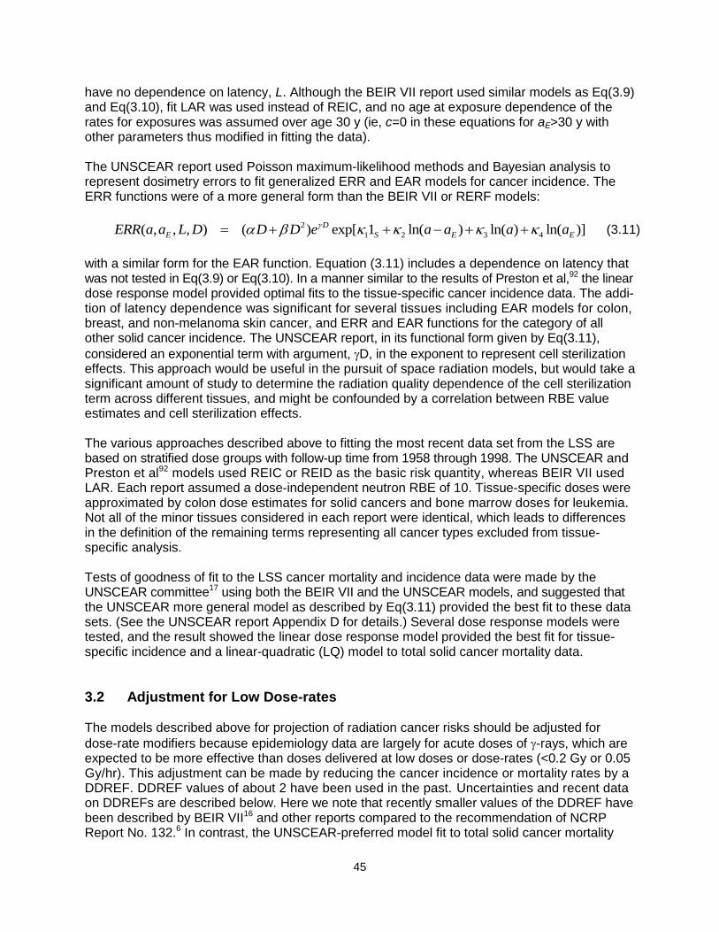
45

have no dependence on latency, L. Although the BEIR VII report used similar models as Eq(3.9) and Eq(3.10), fit LAR was used instead of REIC, and no age at exposure dependence of the rates for exposures was assumed over age 30 y (ie, c=0 in these equations for aE>30 y with other parameters thus modified in fitting the data). The UNSCEAR report used Poisson maximum-likelihood methods and Bayesian analysis to represent dosimetry errors to fit generalized ERR and EAR models for cancer incidence. The ERR functions were of a more general form than the BEIR VII or RERF models:

2

1 2 3 4( , , , ) ( ) exp[ 1 ln( ) ln( ) ln( )]D

E S E EERR a a L D D D e a a a a (3.11)

with a similar form for the EAR function. Equation (3.11) includes a dependence on latency that was not tested in Eq(3.9) or Eq(3.10). In a manner similar to the results of Preston et al,92 the linear dose response model provided optimal fits to the tissue-specific cancer incidence data. The addi-tion of latency dependence was significant for several tissues including EAR models for colon, breast, and non-melanoma skin cancer, and ERR and EAR functions for the category of all other solid cancer incidence. The UNSCEAR report, in its functional form given by Eq(3.11),

considered an exponential term with argument, D, in the exponent to represent cell sterilization effects. This approach would be useful in the pursuit of space radiation models, but would take a significant amount of study to determine the radiation quality dependence of the cell sterilization term across different tissues, and might be confounded by a correlation between RBE value estimates and cell sterilization effects. The various approaches described above to fitting the most recent data set from the LSS are based on stratified dose groups with follow-up time from 1958 through 1998. The UNSCEAR and Preston et al92 models used REIC or REID as the basic risk quantity, whereas BEIR VII used LAR. Each report assumed a dose-independent neutron RBE of 10. Tissue-specific doses were approximated by colon dose estimates for solid cancers and bone marrow doses for leukemia. Not all of the minor tissues considered in each report were identical, which leads to differences in the definition of the remaining terms representing all cancer types excluded from tissue-specific analysis. Tests of goodness of fit to the LSS cancer mortality and incidence data were made by the UNSCEAR committee17 using both the BEIR VII and the UNSCEAR models, and suggested that the UNSCEAR more general model as described by Eq(3.11) provided the best fit to these data sets. (See the UNSCEAR report Appendix D for details.) Several dose response models were tested, and the result showed the linear dose response model provided the best fit for tissue-specific incidence and a linear-quadratic (LQ) model to total solid cancer mortality data.

3.2 Adjustment for Low Dose-rates The models described above for projection of radiation cancer risks should be adjusted for

dose-rate modifiers because epidemiology data are largely for acute doses of -rays, which are expected to be more effective than doses delivered at low doses or dose-rates (<0.2 Gy or 0.05 Gy/hr). This adjustment can be made by reducing the cancer incidence or mortality rates by a DDREF. DDREF values of about 2 have been used in the past. Uncertainties and recent data on DDREFs are described below. Here we note that recently smaller values of the DDREF have been described by BEIR VII16 and other reports compared to the recommendation of NCRP Report No. 132.6 In contrast, the UNSCEAR-preferred model fit to total solid cancer mortality

46

was an LQ dose response model.10,17 An identical approach to leukemia risk estimation could therefore be followed where no DDREF is applied, while the quadratic dose term is ignored for low dose-rates. However, the optimal fit to cancer incidence by UNSCEAR was a linear dose response model, where a DDREF would normally still be applied.

3.3 Comparisons of Tissue-specific Risk Models We compared the BEIR VII,16 UNSCEAR,17 and Preston et al92 model fits for age- and gender-specific REIC and REID probabilities using the 2005 U.S. population data for cancer incidence, mortality, and life-table for all causes of death.99 All calculations are made with a DDREF of 1.75 for solid cancer risks, and the linear component of the leukemia model. The minimum latency for solid cancers is assumed as 5 years, and for leukemia as 2 years for all calculation in this report. Preston et al92 considered several tissues not considered by BEIR VII and UNSCEAR, including tumors of the oral cavity and esophagus. Figures 3.1 and 3.2 compare these models for the %-REIC using identical U.S. population rates from 200599 and a DDREF value of 1.75. Appendix A contains tables of estimates of REIC and REID for several cancer types. In Appendix B, we consider estimates for specific demographic factors within the U.S. population. Lung cancer makes the largest contribution to the risk, and the differences between the additive and the multiplicative models for lung cancer risks are found to be substantial, which is well documented.6 Importantly, the models predict REIC values about 2 times higher than REID, or about a 20% increase compared to the analysis of NCRP Report No. 132.6

3.4 Age at Exposure Dependence of Cancer NCRP Report No. 9898 recommendations to NASA with regard to the age dependence of career dose limits was a substantial change from the contemporary dose limits for astronauts, and was also distinct from radiation protection methods at other government agencies or nations.27 Tables of career limits were calculated for a 10-y career under the assumption that exposures were distributed evenly over the 10-y period,98 and the report noted that more detailed calcu-lations are needed if other career lengths are considered. NCRP Report No. 132 employed sim-ilar methodologies to NCRP Report No. 98, although it used the revised human epidemiology findings that occurred between the publications of the different reports. Table 3.1 compares the age-dependent dose limits from the two reports. The more recent report recommended reducing Effective dose limits by more than 2-fold below age 50 y compared to the former NCRP report. The largest difference between the NCRP estimates from 2000 and the BEIR VII model or recommended NASA 2010 approach is the reduction of the age at exposure dependence of cancer risk estimates and dose limits, with a more than a 3-fold change over the possible ages of astronauts in the NCRP model compared to a less than 50% change in the incidence-based risk transfer model approach. Figure 3.3 compares REID values for solid cancer risk in the two approaches. The upper panels for males and females compares calculations using the rates from LSS report 13, the UNSCEAR mortality fits (linear term only), and the BEIR VII model. The NCRP and BEIR VII calculations use an identical DDREF of 2, and the UNSCEAR result uses the linear

term from an LQ fit with DDREF=1. All calculations use the 2005 U.S. population data and T=0.5 for all tissues. The NCRP and UNSCEAR mortality transport models show a similar dependence on aE, and would be in even closer agreement if the UNSCEAR model were applied with a DDREF of about 1.3, or if the NCRP model DDREF was reduced from 2 to about 1.7. The

47

Figure 3.1. Comparison of %REIC per Sv for males and females as a function of age at exposure for

mixture model U.S. for the BEIR VII, UNSCEAR, and Preston et al92

tissue-specific cancer rates. Left

panels for males; right panels for females.

48

Figure 3.2. Comparison of %REIC per Sv for males and females as a function of age at exposure for

mixture model and for the BEIR VII, UNSCEAR, and Preston et al92

tissue-specific cancer rates. Left

panels for males; right panels for females.

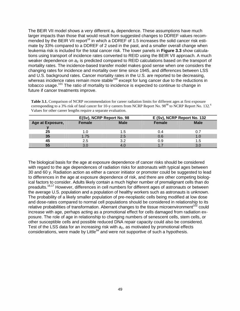
49

The BEIR VII model shows a very different aE dependence. These assumptions have much larger impacts than those that would result from suggested changes to DDREF values recom-mended by the BEIR VII report16 in which a DDREF of 1.5 increases the solid cancer risk esti-mate by 33% compared to a DDREF of 2 used in the past, and a smaller overall change when leukemia risk is included for the total cancer risk. The lower panels in Figure 3.3 show calcula-tions using transport of incidence rates converted to REID using the BEIR VII approach. A much weaker dependence on aE is predicted compared to REID calculations based on the transport of mortality rates. The incidence-based transfer model makes good sense when one considers the changing rates for incidence and mortality over time since 1945, and differences between LSS and U.S. background rates. Cancer mortality rates in the U.S. are reported to be decreasing, whereas incidence rates remain more stable100 except for lung cancer due to the reductions in tobacco usage.101 The ratio of mortality to incidence is expected to continue to change in future if cancer treatments improve.

The biological basis for the age at exposure dependence of cancer risks should be considered with regard to the age dependences of radiation risks for astronauts with typical ages between 30 and 60 y. Radiation action as either a cancer initiator or promoter could be suggested to lead to differences in the age at exposure dependence of risk, and there are other competing biolog-ical factors to consider. Adults likely contain a much higher number of premalignant cells than do preadults.16,17 However, differences in cell numbers for different ages of astronauts or between the average U.S. population and a population of healthy workers such as astronauts is unknown. The probability of a likely smaller population of pre-neoplastic cells being modified at low dose and dose-rates compared to normal cell populations should be considered in relationship to its relative probabilities of transformation. Aberrant changes to the tissue microenvironment102 could increase with age, perhaps acting as a promotional effect for cells damaged from radiation ex-posure. The role of age in relationship to changing numbers of senescent cells, stem cells, or other susceptible cells and possible reduced DNA repair capacity could also be considered. Test of the LSS data for an increasing risk with aE, as motivated by promotional effects considerations, were made by Little94 and were not supportive of such a hypothesis.

Table 3.1. Comparison of NCRP recommendation for career radiation limits for different ages at first exposure

corresponding to a 3% risk of fatal cancer for 10-y careers from NCRP Report No. 9898

to NCRP Report No. 132.6

Values for other career lengths require a separate evaluation.

E(Sv), NCRP Report No. 98 E (Sv), NCRP Report No. 132

Age at Exposure, y

Female Male Female Male

25 1.0 1.5 0.4 0.7 35 1.75 2.5 0.6 1.0 45 2.5 3.2 0.9 1.5 55 3.0 4.0 1.7 3.0

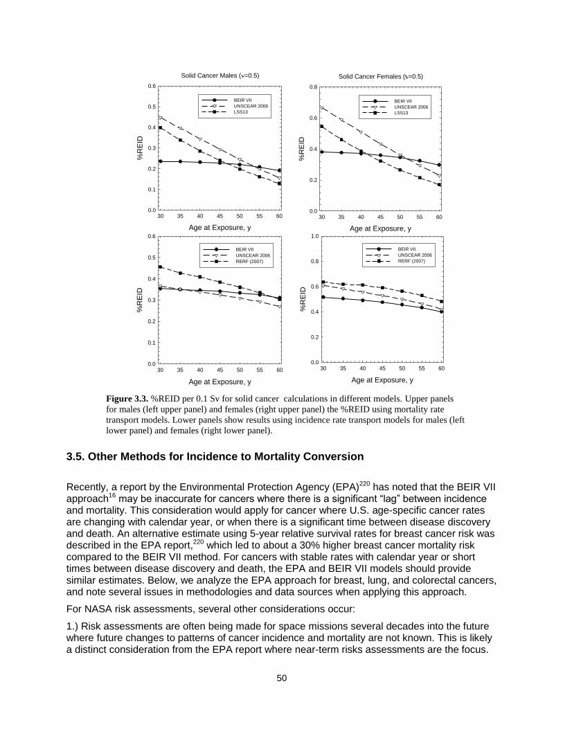
50

3.5. Other Methods for Incidence to Mortality Conversion

Recently, a report by the Environmental Protection Agency (EPA)220 has noted that the BEIR VII approach16 may be inaccurate for cancers where there is a significant ―lag‖ between incidence and mortality. This consideration would apply for cancer where U.S. age-specific cancer rates are changing with calendar year, or when there is a significant time between disease discovery and death. An alternative estimate using 5-year relative survival rates for breast cancer risk was described in the EPA report,220 which led to about a 30% higher breast cancer mortality risk compared to the BEIR VII method. For cancers with stable rates with calendar year or short times between disease discovery and death, the EPA and BEIR VII models should provide similar estimates. Below, we analyze the EPA approach for breast, lung, and colorectal cancers, and note several issues in methodologies and data sources when applying this approach.

For NASA risk assessments, several other considerations occur:

1.) Risk assessments are often being made for space missions several decades into the future where future changes to patterns of cancer incidence and mortality are not known. This is likely a distinct consideration from the EPA report where near-term risks assessments are the focus.

Figure 3.3. %REID per 0.1 Sv for solid cancer calculations in different models. Upper panels

for males (left upper panel) and females (right upper panel) the %REID using mortality rate

transport models. Lower panels show results using incidence rate transport models for males (left

lower panel) and females (right lower panel).

Age at Exposure, y

30 35 40 45 50 55 60

%R

EID

0.0

0.2

0.4

0.6

0.8

1.0

BEIR VII

UNSCEAR 2006

RERF (2007)

Females ( T=0.5)

Age at Exposure, y

30 35 40 45 50 55 60

%R

EID

0.0

0.1

0.2

0.3

0.4

0.5

0.6

BEIR VII

UNSCEAR 2006

RERF (2007)

Males ( T=0.5)

Solid Cancer Males ( =0.5)

Age at Exposure, y

30 35 40 45 50 55 60

%R

EID

0.0

0.1

0.2

0.3

0.4

0.5

0.6

BEIR VII

UNSCEAR 2006

LSS13

Solid Cancer Females ( =0.5)

Age at Exposure, y

30 35 40 45 50 55 60

%R

EID

0.0

0.2

0.4

0.6

0.8

BEIR VII

UNSCEAR 2006

LSS13

51

2.) The EPA used LAR in their report. The EPA method would be more cumbersome to apply using calculations of REID because the probability to survive to a given age depends both on background and on radiation-induced mortality rates in REID estimates, but on background mortality rates alone for LAR estimates.

3.) The healthy worker effects expected for never-smokers and other improved lifestyle factors noted for astronauts could lead to differences in histology’s in cancer that occur and in success of treatments.235 On the other hand, the type of tumors induced by space radiation may be distinct from those in different populations. These considerations could become the focus of future analysis as NASA develops individual-based approaches to reduce risks.

4.) Upon considering the surveillance, epidemiology, and end results (SEER) and other data for incidence, mortality, and 5-year survival probabilities, it is important to note that the disease stage at diagnosis can have a profound impact on the incidence to mortality conversion to be used for astronauts. Table 3.2 shows such data for several cancers where early diagnosis of cancers – namely lung, colon, breast, ovarian, and prostate – has made much progress in recent years. The BEIR VII and EPA approach use conversion coefficients similar to the All (average) category, which has much higher probability of death compared to when early cancer detection occurs. Clearly, a significantly reduced REID probability would be found if early detection at Stage I of these important radiogenic cancers could be assumed by NASA. However, REIC estimates would not be changed by early diagnosis. These are important considerations for risk management that should be considered in the future, especially when high risk missions are considered.

Breast Cancer: We applied the EPA method for different stages of disease discovery to understand how the method compared to the tissue specific cancer mortality rates used in the BEIR VII approach. The EPA method assumes that mortality rates are constant when they estimate breast cancer mortality rates for patients diagnosed with cancer. They make the argument that this is reasonable for the first 10 years after diagnoses based on an article published by Bland et al.237 They used the National Cancer Data Base breast carcinoma data and concluded in the abstract that ―In general, the annual relative survival rate remained constant over the 10 year observation period (with no plateau after 5 years within each stage and for all stages combined.)‖. Cronin et al238 published 5-year and 10-year relative survival rates for breast cancer based separated out into stages. Comparing these rates, a constant mortality rate seems reasonable for local and regional cancers, which are the majority of breast

Table 3.2. 5-year survival probabilities for cancers where early detection programs are partially successful.236

Cancer All (ave) Stage I Stage II Stage III Stage IV

Males (White)

Lung 14% 54% 32% 9% 2%

Colon 67% 97% 84% 63% 8%

Prostate 100% - 100% 100% 50%

Females (White)

Lung 19% 63% 35% 11% 3%

Colon 65% 94% 82% 61% 8%

Breast 90% 100% 90% 62% 23%

Ovarian 46% 94% 73% 28% 22%

52

cancers (only 7% are distant or unknown). In the EPA model, incidence was followed for 10 years to predict mortality rates. Extending this assumption past 10 years would be more uncertain. Figure 3.5 shows comparisons of the EPA model to the SEER breast cancer mortality rates. All stages uses the relative survival rates estimated using all stages of cancer separated into age groups for diagnosis. Localized uses the relative survival rates for localized cancer separated into age groups for diagnosis and provides an estimate for the mortality rate if all breast cancer incidences were localized. Similarly regional, distant, and unknown relative survival rates were implemented. The average weighted by stage distribution, averaged the four stages of cancer using the following stage distribution: Localized = %60, Regional = %33, Distant = %5, and unknown = %2. The All stages and average weighted by stage estimates overlap each other. This means that it would be unnecessary to separate out the stages when estimating the REID for breast cancer. The estimates are not smoothed due to the categorical nature of the age groups for relative survival rates. The mortality rates are well predicted up to about age 70 when all stages are combined. Since the relative survival rates adjust for the normal mortality that the cohort would experience from other causes of death, the lower estimates at older ages could be due to using relative survival rates. At older ages, some breast cancer deaths may not be counted because of the high probability that they would have died from another cause. The lower mortality rate estimates explain the REID decreasing from 0.43 to 0.32 for radiation exposures at age 35 when the EPA method was applied. Analysis showed the REID decreased when the EPA method was applied for less than 15 years. The REID has slight increases as more years are followed. The REID only becomes larger than the BEIR VII method after 20 years of incidence are followed for those exposed at ages less than 45. The EPA estimates the LAR to be 30% larger than the estimate of BEIR VII. We do not find the large increase that the EPA found. However, we have updated the incidence, mortality, and relative survival rates compared to their report. The differences could be due to the breast cancer incidence rates leveling off in the last 10 years as seen in Figure 3.5, unlike the increases seen between 1980 and 2000. With less changes in incidence rate over time, the two methods' results should become more similar to each other.

Table 3.3. Results for mortality probability following incidence for 5, 10, 15, and 20 years after

diagnosis to REID estimates from NSCR 2012 model.

Age at Exposure, y

Model 30 35 40 45 50 55 60

NASA2010 0.561 0.433 0.331 0.251 0.183 0.132 0.094

BrEPA5 0.267 0.202 0.150 0.111 0.077 0.053 0.035

BrEPA10 0.424 0.320 0.237 0.175 0.120 0.080 0.052

BrEPA15 0.537 0.405 0.299 0.219 0.148 0.098 0.062

BrEPA20 0.617 0.464 0.341 0.248 0.166 0.108 0.067

53

Figure 3.5. Comparisons of breast cancer mortality rates for different stages of disease discovery using US-EPA

method to SEER mortality rates for 10-year follow up times (top left panel). Comparisons of breast cancer

mortality rates using US-EPA method to SEER mortality rates for 10-, 15-, and 20-year follow-up times using two

different methods to combine different stages of disease discovery (top right panel). Lower panel shows the age

adjusted breast cancer incidence and mortality rates versus calendar year from SEER.

54

Colon and Rectum Cancer: Cronin et al238 also published 5-year and 10-year relative survival rates for colon and rectum cancer. The constant hazard rates over 10 years is only a reasonable assumption for localized colon cancer, which is 39% of colon cancers. Incidence was followed up to 5 years and compared with observed mortality rates to determine whether a constant hazard rate might be reasonable for the first 5 years (Figure 3.6). The mortality rate is well predicted up to age 80 y. Again, the lower mortality rate at older ages causes the REID to decrease from 0.44 to 0.42 for females and 0.51 to 0.45 for males exposed at age 35. Following localized cancer incidence up to 10 years was also considered in the right side figures.

Figure 3.6. Comparisons of colon cancer mortality rates for different stages of disease discovery using US-EPA

method to SEER mortality rates for 5-year follow-up times (left panels). Comparisons of colon cancer mortality

rates using US-EPA method to SEER mortality rates for 5 years, and 10 years for localized cancers, follow up

times using two different methods to combine different stages of disease discovery (right panels). Top panels

for females and lower panels for males.

Female

Male

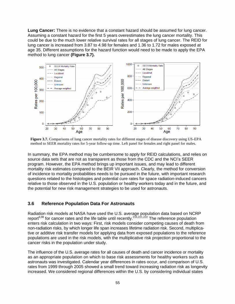
55

Lung Cancer: There is no evidence that a constant hazard should be assumed for lung cancer.

Assuming a constant hazard for the first 5 years overestimates the lung cancer mortality. This could be due to the much lower relative survival rates for all stages of lung cancer. The REID for lung cancer is increased from 3.87 to 4.98 for females and 1.36 to 1.72 for males exposed at age 35. Different assumptions for the hazard function would need to be made to apply the EPA method to lung cancer (Figure 3.7).

In summary, the EPA method may be cumbersome to apply for REID calculations, and relies on source data sets that are not as transparent as those from the CDC and the NCI’s SEER program. However, the EPA method brings up important issues, and may lead to different mortality risk estimates compared to the BEIR VII approach. Clearly, the method for conversion of incidence to mortality probabilities needs to be pursued in the future, with important research questions related to the histologies and potential cure rates for space radiation-induced cancers relative to those observed in the U.S. population or healthy workers today and in the future, and the potential for new risk management strategies to be used for astronauts.

3.6 Reference Population Data For Astronauts Radiation risk models at NASA have used the U.S. average population data based on NCRP report6,98 for cancer rates and the life table until recently.215,221,222 The reference population enters risk calculation in two ways: First, risk models consider competing causes of death from non-radiation risks, by which longer life span increases lifetime radiation risk. Second, multiplica-tive or additive risk transfer models for applying data from exposed populations to the reference populations are used in the risk models, with the multiplicative risk projection proportional to the cancer risks in the population under study.

The influence of the U.S. average rates for all causes of death and cancer incidence or mortality as an appropriate population on which to base risk assessments for healthy workers such as astronauts was investigated. Calendar year differences in rates occur, and comparison of U.S. rates from 1999 through 2005 showed a small trend toward increasing radiation risk as longevity increased. We considered regional differences within the U.S. by considering individual states

Figure 3.7. Comparisons of lung cancer mortality rates for different stages of disease discovery using US-EPA

method to SEER mortality rates for 5-year follow-up time. Left panel for females and right panel for males.

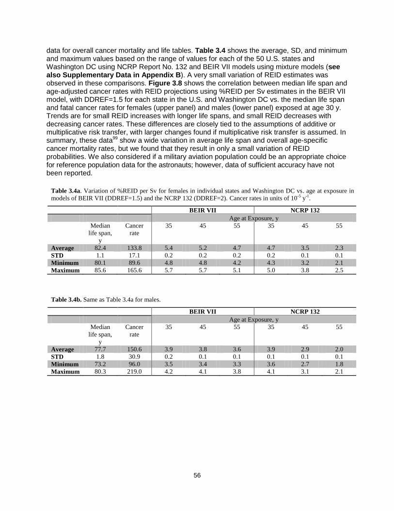
56

data for overall cancer mortality and life tables. Table 3.4 shows the average, SD, and minimum and maximum values based on the range of values for each of the 50 U.S. states and Washington DC using NCRP Report No. 132 and BEIR VII models using mixture models (see also Supplementary Data in Appendix B). A very small variation of REID estimates was observed in these comparisons. Figure 3.8 shows the correlation between median life span and age-adjusted cancer rates with REID projections using %REID per Sv estimates in the BEIR VII model, with DDREF=1.5 for each state in the U.S. and Washington DC vs. the median life span and fatal cancer rates for females (upper panel) and males (lower panel) exposed at age 30 y. Trends are for small REID increases with longer life spans, and small REID decreases with decreasing cancer rates. These differences are closely tied to the assumptions of additive or multiplicative risk transfer, with larger changes found if multiplicative risk transfer is assumed. In summary, these data99 show a wide variation in average life span and overall age-specific cancer mortality rates, but we found that they result in only a small variation of REID probabilities. We also considered if a military aviation population could be an appropriate choice for reference population data for the astronauts; however, data of sufficient accuracy have not been reported.

Table 3.4b. Same as Table 3.4a for males.

BEIR VII NCRP 132

Age at Exposure, y

Median

life span,

y

Cancer

rate

35 45 55 35 45 55

Average 77.7 150.6 3.9 3.8 3.6 3.9 2.9 2.0

STD 1.8 30.9 0.2 0.1 0.1 0.1 0.1 0.1

Minimum 73.2 96.0 3.5 3.4 3.3 3.6 2.7 1.8

Maximum 80.3 219.0 4.2 4.1 3.8 4.1 3.1 2.1

Table 3.4a. Variation of %REID per Sv for females in individual states and Washington DC vs. age at exposure in

models of BEIR VII (DDREF=1.5) and the NCRP 132 (DDREF=2). Cancer rates in units of 10-5

y-1

.

BEIR VII NCRP 132

Age at Exposure, y

Median

life span,

y

Cancer

rate

35 45 55 35 45 55

Average 82.4 133.8 5.4 5.2 4.7 4.7 3.5 2.3

STD 1.1 17.1 0.2 0.2 0.2 0.2 0.1 0.1

Minimum 80.1 89.6 4.8 4.8 4.2 4.3 3.2 2.1

Maximum 85.6 165.6 5.7 5.7 5.1 5.0 3.8 2.5

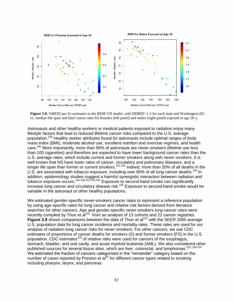
57

Astronauts and other healthy workers or medical patients exposed to radiation enjoy many lifestyle factors that lead to reduced lifetime cancer risks compared to the U.S. average population.239 Healthy worker attributes found for astronauts include optimal ranges of body mass index (BMI), moderate alcohol use, excellent nutrition and exercise regimes, and health care.240 More importantly, more than 90% of astronauts are never-smokers (lifetime use less than 100 cigarettes) and therefore are expected to have lower background cancer rates than the U.S. average rates, which include current and former smokers along with never-smokers. It is well known that NS have lower rates of cancer, circulatory and pulmonary diseases, and a longer life span than former or current smokers.241,242 Indeed, more than 20% of all deaths in the U.S. are associated with tobacco exposure, including over 80% of all lung cancer deaths.105 In addition, epidemiology studies suggest a harmful synergistic interaction between radiation and tobacco exposure occurs.104,109,222,243,244 Exposure to second-hand smoke can significantly increase lung cancer and circulatory disease risk.105 Exposure to second-hand smoke would be variable in the astronaut or other healthy populations.

We estimated gender-specific never-smokers cancer rates to represent a reference population by using age-specific rates for lung cancer and relative risk factors derived from literature searches for other cancers. Age and gender-specific never-smokers lung cancer rates were recently compiled by Thun et al103 from an analysis of 13 cohorts and 22 cancer registries. Figure 3.9 shows comparisons between the data of Thun et al103 with the SEER 2005 average U.S. population data for lung cancer incidence and mortality rates. These rates are used for our analysis of radiation lung cancer risks for never-smokers. For other cancers, we use CDC estimates of proportions of cancer deaths for smokers (S) and former smokers (FS) in the U.S. population. CDC estimates105 of relative risks were used for cancers of the esophagus, stomach, bladder, and oral cavity, and acute myeloid leukemia (AML). We also considered other published sources for several tissue sites, which are liver, colorectal, and lymphomas.223, 245-247 We estimated the fraction of cancers categorized in the ―remainder‖ category based on the number of cases reported by Preston et al92 for different cancer types related to smoking including pharynx, larynx, and pancreas.

Figure 3.8. %REID per Sv estimates in the BEIR VII model, with DDREF=1.5 for each state and Washington DC

vs. median life span and fatal cancer rates for females (left panel) and males (right panel) exposed at age 30 y.

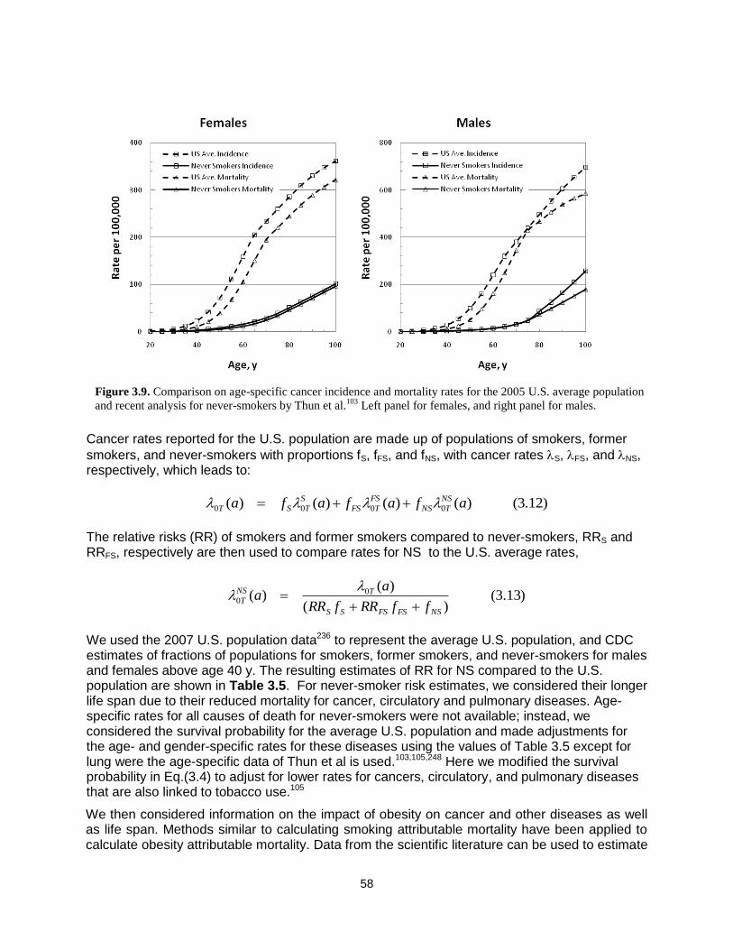
58

Cancer rates reported for the U.S. population are made up of populations of smokers, former

smokers, and never-smokers with proportions fS, fFS, and fNS, with cancer rates S, FS, and NS, respectively, which leads to:

)12.3()()()()( 0000 afafafa NS

TNS

FS

TFS

S

TST

The relative risks (RR) of smokers and former smokers compared to never-smokers, RRS and RRFS, respectively are then used to compare rates for NS to the U.S. average rates,

)13.3()(

)()( 0

0

NSFSFSSS

TNS

TffRRfRR

aa

We used the 2007 U.S. population data236 to represent the average U.S. population, and CDC estimates of fractions of populations for smokers, former smokers, and never-smokers for males and females above age 40 y. The resulting estimates of RR for NS compared to the U.S. population are shown in Table 3.5. For never-smoker risk estimates, we considered their longer life span due to their reduced mortality for cancer, circulatory and pulmonary diseases. Age-specific rates for all causes of death for never-smokers were not available; instead, we considered the survival probability for the average U.S. population and made adjustments for the age- and gender-specific rates for these diseases using the values of Table 3.5 except for lung were the age-specific data of Thun et al is used.103,105,248 Here we modified the survival probability in Eq.(3.4) to adjust for lower rates for cancers, circulatory, and pulmonary diseases that are also linked to tobacco use.105

We then considered information on the impact of obesity on cancer and other diseases as well as life span. Methods similar to calculating smoking attributable mortality have been applied to calculate obesity attributable mortality. Data from the scientific literature can be used to estimate

Figure 3.9. Comparison on age-specific cancer incidence and mortality rates for the 2005 U.S. average population

and recent analysis for never-smokers by Thun et al.103

Left panel for females, and right panel for males.

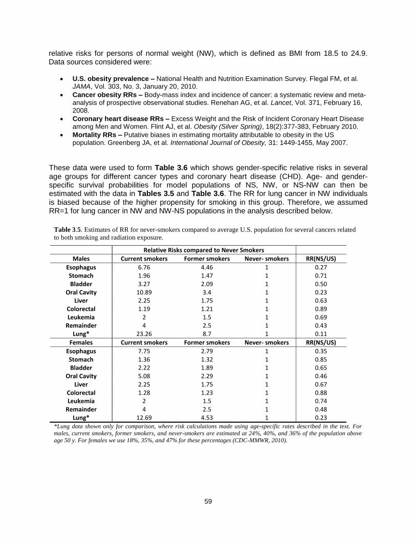
59

relative risks for persons of normal weight (NW), which is defined as BMI from 18.5 to 24.9. Data sources considered were:

U.S. obesity prevalence – National Health and Nutrition Examination Survey. Flegal FM, et al. JAMA, Vol. 303, No. 3, January 20, 2010.

Cancer obesity RRs – Body-mass index and incidence of cancer: a systematic review and meta-analysis of prospective observational studies. Renehan AG, et al. Lancet, Vol. 371, February 16, 2008.

Coronary heart disease RRs – Excess Weight and the Risk of Incident Coronary Heart Disease among Men and Women. Flint AJ, et al. Obesity (Silver Spring), 18(2):377-383, February 2010.

Mortality RRs – Putative biases in estimating mortality attributable to obesity in the US population. Greenberg JA, et al. International Journal of Obesity, 31: 1449-1455, May 2007.

These data were used to form Table 3.6 which shows gender-specific relative risks in several age groups for different cancer types and coronary heart disease (CHD). Age- and gender-specific survival probabilities for model populations of NS, NW, or NS-NW can then be estimated with the data in Tables 3.5 and Table 3.6. The RR for lung cancer in NW individuals is biased because of the higher propensity for smoking in this group. Therefore, we assumed RR=1 for lung cancer in NW and NW-NS populations in the analysis described below.

Table 3.5. Estimates of RR for never-smokers compared to average U.S. population for several cancers related

to both smoking and radiation exposure.

Relative Risks compared to Never Smokers

Males Current smokers Former smokers Never- smokers RR(NS/US)

Esophagus 6.76 4.46 1 0.27 Stomach 1.96 1.47 1 0.71 Bladder 3.27 2.09 1 0.50

Oral Cavity 10.89 3.4 1 0.23 Liver 2.25 1.75 1 0.63

Colorectal 1.19 1.21 1 0.89 Leukemia 2 1.5 1 0.69

Remainder 4 2.5 1 0.43 Lung* 23.26 8.7 1 0.11

Females Current smokers Former smokers Never- smokers RR(NS/US)

Esophagus 7.75 2.79 1 0.35 Stomach 1.36 1.32 1 0.85 Bladder 2.22 1.89 1 0.65

Oral Cavity 5.08 2.29 1 0.46 Liver 2.25 1.75 1 0.67

Colorectal 1.28 1.23 1 0.88 Leukemia 2 1.5 1 0.74

Remainder 4 2.5 1 0.48 Lung* 12.69 4.53 1 0.23

*Lung data shown only for comparison, where risk calculations made using age-specific rates described in the text. For

males, current smokers, former smokers, and never-smokers are estimated at 24%, 40%, and 36% of the population above

age 50 y. For females we use 18%, 35%, and 47% for these percentages (CDC-MMWR, 2010).

60

Evidence that astronauts should be considered to be at lower risk for cancers and circulatory diseases, and enjoy a longer life span compared to the U.S. average population is borne out by analysis of Kaplan-Meir survival curves (Figure 3.10) and Standard Mortality Ratios (SMRs) (Table 3.7), where the cohort of NASA astronauts and payload specialists is compared to the U.S. average population, and our estimates for NS, NW, or NS-NW model populations. These comparisons include results after censoring 18 of 19 occupationally related accidental deaths from space missions or training considered atypical of U.S. workers. The largely male cohort of astronauts and payload specialists show a longer longevity and reduced SMR in comparison to the U.S. average population, and are more similar to a population of never-smokers with normal weight, which is a strong indication that a healthy worker effect occurs for astronauts. It is possible but not likely that the population effective dose (over 100 Sv for the astronaut cohort 7,30) has led to any increase in cancers at this time because of the small cohort size and because the current average of the astronaut population is only 59 y, such that the observation time after exposure is still relatively short.

Table 3.6. Relative risks for NW persons compared to the U.S. average for males and females for cancer and CHD.

Cause 20 to 39 40 to 59 > 60 y 20 to 39 40 to 59 >60 y

Leukemia 0.923 0.907 0.904 0.825 0.810 0.823

Colon 0.788 0.751 0.746 0.903 0.894 0.902

Liver 0.788 0.751 0.746 0.924 0.917 0.923

Lung 1.275 1.361 1.373 1.246 1.280 1.263

Esophagus 0.602 0.551 0.543 0.560 0.538 0.567

Thyroid 0.722 0.678 0.671 0.853 0.841 0.852

Kidney 0.788 0.751 0.746 0.679 0.659 0.681

Gallbladder 0.914 0.896 0.893 0.512 0.490 0.521

NHL 0.942 0.929 0.927 0.924 0.917 0.923

Breast(PostM)* 0.873 0.862 0.871

Breast(PreM) 1.093 1.104 1.097

Prostate 0.970 0.964 0.963

CHD 0.725 0.682 0.677 0.675 0.650 0.659

Mortality 0.863 0.836 0.829 0.833 0.819 0.839

*PostM and PreM for post-menopause or pre-menopause, respectively.

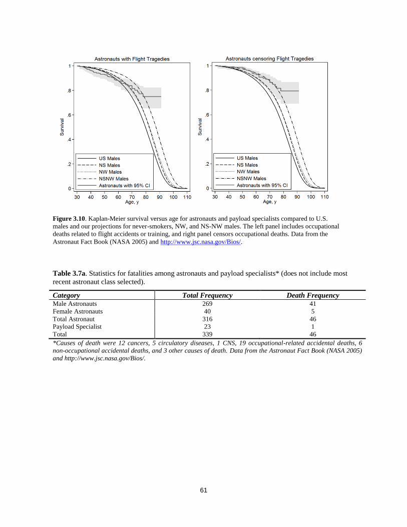
61

Table 3.7a. Statistics for fatalities among astronauts and payload specialists* (does not include most

recent astronaut class selected).

Category Total Frequency Death Frequency Male Astronauts 269 41

Female Astronauts 40 5

Total Astronaut 316 46

Payload Specialist 23 1

Total 339 46

*Causes of death were 12 cancers, 5 circulatory diseases, 1 CNS, 19 occupational-related accidental deaths, 6

non-occupational accidental deaths, and 3 other causes of death. Data from the Astronaut Fact Book (NASA 2005)

and http://www.jsc.nasa.gov/Bios/.

Figure 3.10. Kaplan-Meier survival versus age for astronauts and payload specialists compared to U.S.

males and our projections for never-smokers, NW, and NS-NW males. The left panel includes occupational

deaths related to flight accidents or training, and right panel censors occupational deaths. Data from the

Astronaut Fact Book (NASA 2005) and http://www.jsc.nasa.gov/Bios/.

http://www.jsc.nasa.gov/Bios/

62

3.6.1. Healthy Worker Effects and Risk Estimates We used NS and U.S. average population rates to estimate lung cancer risks using the BEIR VII, UNSCEAR, and RERF models as shown in Tables 3.8 and 3.9 for estimates of REIC and REID, respectively. A significant decrease in REID and REIC probabilities for never-smokers compared to the average U.S. population was estimated for lung cancer risks when multiplicative risk transfer is assumed. A more than 8-fold decrease is estimated in the multiplicative transfer model when never-smoker rates are compared to the U.S. population average. Using a mixture model with vT=0.5 reduced the lung cancer estimate for never-smokers by 2-fold compared to the average U.S. population. The generalized multiplicative model of Furukawa et al,104 which estimates radiation risks dependent on smoking consumption leads to a minor reduction for females compared to the usage of never-smoker baseline rate estimates alone, and is about the same for males. We note that Furukawa et al104 used lung dose estimates for the LSS cohort, while the reports noted above used colon doses to represent all solid cancer risks including the risk of lung cancer. Because lung cancer is the largest contributor to overall radiation cancer risks, these lower estimates for never-smokers have large impacts on overall risk estimates.

Table 3.7d. Standard Mortality Ratio (SMR) for astronauts and payload specialists relative

to model other populations for coronary heart disease and stroke.

Comparison SMR Astronauts vs. U.S. avg. 0.33 [0.14, 0.80]

Astronauts vs. NS avg. 0.43 [0.18, 1.04]

Astronauts vs NW avg. 0.47 [0.19, 1.12]

Astronauts vs NS-NW Avg. 0.67 [0.28, 1.62]

Table 3.7c. Standard Cancer Mortality Ratio (SMR) for astronauts and payload specialists

relative to other populations for cancer.





Table 3.7b. Standard Mortality Ratio (SMR) for astronauts and payload specialists relative

to U.S. average or never-smokers average (gender weighted to proportion of M and F

astronauts) or female never-smokers, suggests astronauts have lifetime risks similar to

female never-smokers.


Censoring tragedies vs. US avg. 0.44 [0.31, 0.63]


Censoring tragedies vs. NS avg. 0.56 [0.39, 0.80]


Censoring tragedies vs NW avg. 0.56 [0.39, 0.80]


Censoring Tragedies vs. NS-NW Avg. 0.93 [0.63, 1.31]

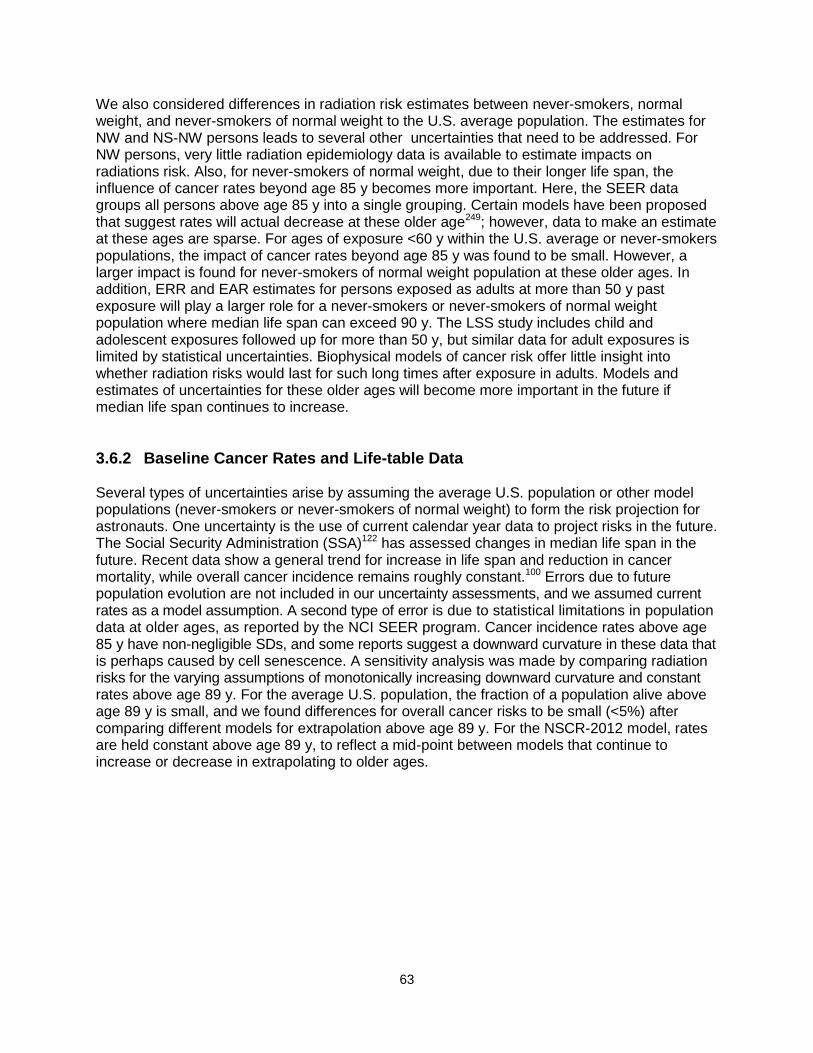
63

We also considered differences in radiation risk estimates between never-smokers, normal weight, and never-smokers of normal weight to the U.S. average population. The estimates for NW and NS-NW persons leads to several other uncertainties that need to be addressed. For NW persons, very little radiation epidemiology data is available to estimate impacts on radiations risk. Also, for never-smokers of normal weight, due to their longer life span, the influence of cancer rates beyond age 85 y becomes more important. Here, the SEER data groups all persons above age 85 y into a single grouping. Certain models have been proposed that suggest rates will actual decrease at these older age249; however, data to make an estimate at these ages are sparse. For ages of exposure <60 y within the U.S. average or never-smokers populations, the impact of cancer rates beyond age 85 y was found to be small. However, a larger impact is found for never-smokers of normal weight population at these older ages. In addition, ERR and EAR estimates for persons exposed as adults at more than 50 y past exposure will play a larger role for a never-smokers or never-smokers of normal weight population where median life span can exceed 90 y. The LSS study includes child and adolescent exposures followed up for more than 50 y, but similar data for adult exposures is limited by statistical uncertainties. Biophysical models of cancer risk offer little insight into whether radiation risks would last for such long times after exposure in adults. Models and estimates of uncertainties for these older ages will become more important in the future if median life span continues to increase.

3.6.2 Baseline Cancer Rates and Life-table Data Several types of uncertainties arise by assuming the average U.S. population or other model populations (never-smokers or never-smokers of normal weight) to form the risk projection for astronauts. One uncertainty is the use of current calendar year data to project risks in the future. The Social Security Administration (SSA)122 has assessed changes in median life span in the future. Recent data show a general trend for increase in life span and reduction in cancer mortality, while overall cancer incidence remains roughly constant.100 Errors due to future population evolution are not included in our uncertainty assessments, and we assumed current rates as a model assumption. A second type of error is due to statistical limitations in population data at older ages, as reported by the NCI SEER program. Cancer incidence rates above age 85 y have non-negligible SDs, and some reports suggest a downward curvature in these data that is perhaps caused by cell senescence. A sensitivity analysis was made by comparing radiation risks for the varying assumptions of monotonically increasing downward curvature and constant rates above age 89 y. For the average U.S. population, the fraction of a population alive above age 89 y is small, and we found differences for overall cancer risks to be small (<5%) after comparing different models for extrapolation above age 89 y. For the NSCR-2012 model, rates are held constant above age 89 y, to reflect a mid-point between models that continue to increase or decrease in extrapolating to older ages.

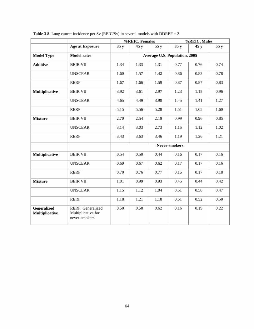
64

Table 3.8. Lung cancer incidence per Sv (REIC/Sv) in several models with DDREF = 2.

%REIC, Females %REIC, Males

Age at Exposure 35 y 45 y 55 y 35 y 45 y 55 y

Model Type Model rates Average U.S. Population, 2005

Additive BEIR VII 1.34 1.33 1.31 0.77 0.76 0.74

UNSCEAR 1.60 1.57 1.42 0.86 0.83 0.78

RERF 1.67 1.66 1.59 0.87 0.87 0.83

Multiplicative BEIR VII 3.92 3.61 2.97 1.23 1.15 0.96

UNSCEAR 4.65 4.49 3.98 1.45 1.41 1.27

RERF 5.15 5.56 5.28 1.51 1.65 1.60

Mixture BEIR VII 2.70 2.54 2.19 0.99 0.96 0.85

UNSCEAR 3.14 3.03 2.73 1.15 1.12 1.02

RERF 3.43 3.63 3.46 1.19 1.26 1.21

Never-smokers


UNSCEAR 0.69 0.67 0.62 0.17 0.17 0.16

RERF 0.70 0.76 0.77 0.15 0.17 0.18

Mixture BEIR VII 1.01 0.99 0.93 0.45 0.44 0.42

UNSCEAR 1.15 1.12 1.04 0.51 0.50 0.47

RERF 1.18 1.21 1.18 0.51 0.52 0.50

Generalized

Multiplicative

RERF, Generalized

Multiplicative for

never-smokers

0.50 0.58 0.62 0.16 0.19 0.22

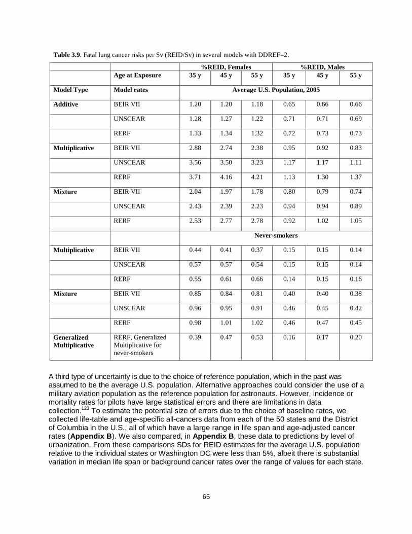
65

A third type of uncertainty is due to the choice of reference population, which in the past was assumed to be the average U.S. population. Alternative approaches could consider the use of a military aviation population as the reference population for astronauts. However, incidence or mortality rates for pilots have large statistical errors and there are limitations in data collection.123 To estimate the potential size of errors due to the choice of baseline rates, we collected life-table and age-specific all-cancers data from each of the 50 states and the District of Columbia in the U.S., all of which have a large range in life span and age-adjusted cancer rates (Appendix B). We also compared, in Appendix B, these data to predictions by level of urbanization. From these comparisons SDs for REID estimates for the average U.S. population relative to the individual states or Washington DC were less than 5%, albeit there is substantial variation in median life span or background cancer rates over the range of values for each state.

Table 3.9. Fatal lung cancer risks per Sv (REID/Sv) in several models with DDREF=2.

%REID, Females %REID, Males

Age at Exposure 35 y 45 y 55 y 35 y 45 y 55 y

Model Type Model rates Average U.S. Population, 2005

Additive BEIR VII 1.20 1.20 1.18 0.65 0.66 0.66

UNSCEAR 1.28 1.27 1.22 0.71 0.71 0.69

RERF 1.33 1.34 1.32 0.72 0.73 0.73


UNSCEAR 3.56 3.50 3.23 1.17 1.17 1.11

RERF 3.71 4.16 4.21 1.13 1.30 1.37

Mixture BEIR VII 2.04 1.97 1.78 0.80 0.79 0.74

UNSCEAR 2.43 2.39 2.23 0.94 0.94 0.89

RERF 2.53 2.77 2.78 0.92 1.02 1.05

Never-smokers


UNSCEAR 0.57 0.57 0.54 0.15 0.15 0.14

RERF 0.55 0.61 0.66 0.14 0.15 0.16

Mixture BEIR VII 0.85 0.84 0.81 0.40 0.40 0.38

UNSCEAR 0.96 0.95 0.91 0.46 0.45 0.42

RERF 0.98 1.01 1.02 0.46 0.47 0.45

Generalized

Multiplicative

RERF, Generalized

Multiplicative for

never-smokers

0.39 0.47 0.53 0.16 0.17 0.20

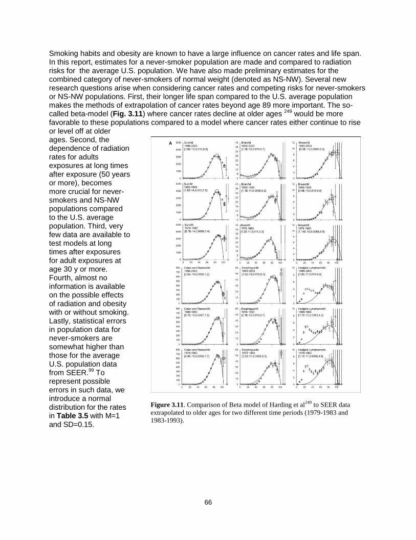
66

Smoking habits and obesity are known to have a large influence on cancer rates and life span. In this report, estimates for a never-smoker population are made and compared to radiation risks for the average U.S. population. We have also made preliminary estimates for the combined category of never-smokers of normal weight (denoted as NS-NW). Several new research questions arise when considering cancer rates and competing risks for never-smokers or NS-NW populations. First, their longer life span compared to the U.S. average population makes the methods of extrapolation of cancer rates beyond age 89 more important. The so-called beta-model (Fig. 3.11) where cancer rates decline at older ages 249 would be more favorable to these populations compared to a model where cancer rates either continue to rise or level off at older ages. Second, the dependence of radiation rates for adults exposures at long times after exposure (50 years or more), becomes more crucial for never-smokers and NS-NW populations compared to the U.S. average population. Third, very few data are available to test models at long times after exposures for adult exposures at age 30 y or more. Fourth, almost no information is available on the possible effects of radiation and obesity with or without smoking. Lastly, statistical errors in population data for never-smokers are somewhat higher than those for the average U.S. population data from SEER.99 To represent possible errors in such data, we introduce a normal distribution for the rates in Table 3.5 with M=1 and SD=0.15.

Figure 3.11. Comparison of Beta model of Harding et al249

to SEER data

extrapolated to older ages for two different time periods (1979-1983 and

1983-1993).

67

3.7 Summary of Research Needs for Type I Uncertainties

1. Models of incidence-to-mortality conversion can be investigated based on possibility of early cancer detection and more aggressive tumor histology by HZE particles and neutrons.

2. Epidemiology data for radiation cancer risks as it is reported by NCI, UNSCEAR, and others should be considered for future integration into NASA risk models.

3. The extrapolation of cancer rates to older ages (> 85 yr) should be investigated. 4. Possible interactions between radiation and tobacco products should be investigated for

their potential role as confounders to human epidemiology data and for risk assessment for astronauts that are former or current smokers.

5. Additional healthy worker effects should be investigated to define the optimal model population to represent astronauts.

68

4. Uncertainties in Low-linear-energy-transfer Risk Model Factors NCRP Report No. 12615 reviewed uncertainties for low-LET radiation risk assessments, and the recommended PDFs were used by NASA for its previous space radiation risk assessments.14,21 Several reports published since 1997, as noted above, provide new sources of information to update uncertainty assessments. We first summarize NCRP Report No. 126 and then describe other information to update the low-LET uncertainty PDFs. For Monte-Carlo sampling purposes,

the low-LET mortality rate per Sievert, L, is written as

Dr

UBTSDE

ELx

xxxxx

DDREF

aaaaE

),(),,( 0 (4.1)

where 0 is the baseline mortality rate per Sievert and the xα are quantiles (random variables)

whose values are sampled from an associated PDF, P(x). Note that the DDREF applies only to the solid cancer risk and not to the leukemia risk under the given assumptions. NCRP Report

No. 12615 defined the following subjective PDFs, P(x), for each factor that contributes to the low-LET-risk projection:

1) Pdosimetry represents random and systematic errors in the estimation of doses received by atomic-bomb blast survivors. It was assumed by the NCRP as a normally distributed PDF for bias correction of random and systematic errors in the dosimetry (DS86) with a mean of 0.84 and an SD of 0.11.

2) Pstatistical represents the distribution in uncertainty in the risk coefficient r0. It is assumed as a normally distributed PDF with a mean of 1 and an SD of 0.15.

3) Pbias represents any bias resulting for over-reporting or underreporting of cancer deaths. Pbias is assumed as a normal distribution with a most probable value of 1.1 and a 90% CI from 1.02 to 1.18 corresponding to an SD of 0.05.

4) Ptransfer represents the uncertainty in the transfer of cancer risk following radiation exposure from the Japanese population to the U.S. population. Both additive and relative risks models were considered by NCRP Report No. 12615 in assessing the uncertainties in such transfer. Ptransfer is log-normal with a mean of 1 and an SD of 0.26 (GSD [geometric standard deviation]=1.3).

5) PDr represents the uncertainty in the knowledge of the extrapolation of risks to low dose and dose-rates embodied in the DDREF. The NCRP assumed PDr to be a truncated triangle distribution starting at 1 and ending at 5 with a peak at 2 and a relative value of ¼ or ½ at 1 or 5, respectively, compared to the peak values for the DDREF at 2. This PDF is used to scale the low-LET risk coefficient (mortality rates) in our estimates for space radiation.

6) PU represents unknown uncertainties. The NCRP assumed this uncertainty followed a normal distribution with a central value of 1 and an SD of 0.3 with 90th-percentile sub-jective CIs of [0.5, 1.5].

The NCRP also considered a PDF for bias correction in projection of cancer risks over a lifetime, which is important for those exposed below age 30 y but not for astronauts. The lifetime projection and NCRP-unknown uncertainties were ignored in the previous NASA model. The analysis and data for updating low-LET cancer risk assessments and uncertainties since NCRP Reports Nos. 126 and 132 are as follows:

69

1) Publication of the revised atomic-bomb dosimetry assessment96 for the LSS of survivor

called dosimetry system 2002 (DS02). 2) Longer follow-up and reanalysis of the LSS cancer incidence data by BEIR VII,16

UNSCEAR17 (see also Little et al10), and Preston et al.92 3) Meta-analysis of other human epidemiology models for breast and thyroid cancer risks

(BEIR VII). 4) Development of EB and Bayesian models for tissue-specific cancer incidence data that

represent significantly reduced tissue-specific statistical errors,95,111 respectively. 5) Assessment of dose response models fitted to human data sets and in the evaluation of

DDREF values, including the BEIR VII analysis16 and analysis of radiation worker studies that support a DDREF value near unity.97

4.1 Life-span Study Dosimetry Errors Errors in dosimetry related to epidemiology data include random and systematic errors. The completion of the revised dosimetry of the atomic-bomb survivors, called dosimetry system 2002, DS02,94 led to minor reductions in the neutron dose estimates as well as modest changes

in estimates of the -ray organ doses compared to the earlier DS86. Recent analysis by BEIR VII, UNSCEAR, and Preston et al112 assume larger dosimetry errors than that of NCRP Report No. 126.15 The DS86 evaluation was subjectively assessed in light of the anticipated dosimetry reevaluation that cumulated in the newer DS02 system. The UNSCEAR report made a Bayesian analysis of dosimetry errors.10,17 Preston et al92 assume an overall 35% error in DS02 estimates. UNSCEAR assumed a log-normal distribution with a GSD of 30%. Other reports112-114 estimate the impact of using a fixed-neutron RBE of 10 in fitting the A-bomb data and other errors. Here, since a larger RBE value and a dose-dependent value are plausible, especially for solid cancers

based on radiobiology experiments with cells and small animals, an overall reduction in the -ray-derived risk coefficients would be expected. A dose-dependent RBE tested by Suzuki et al112

indicated that reductions as high as 30% in the -ray risks were plausible if the neutron RBE ac-tually had a much higher value than the 10 that was assumed in recent reports. Another source of error is the use of stratified dose groups instead of individualized dose estimates.10 Tissue sites in which meta-analysis over several exposed cohorts is considered introduces other dosimetry considerations. Cohorts exposed for medical conditions often involved x-ray exposures that have

RBEs of two or more compared to -rays at low doses.115-117 Underreporting of doses from other sources is also a potential bias. After considering these various descriptions and the previous NCRP Report No. 126 assessment, we assume a log-normal PDF for the combined dosim-etry uncertainties with a geometric mean of 0.9 and GSD of 1.3. This represents a signifi-cant increase in dosimetry error compared to the NCRP Report No. 126 recommendation.

4.2 Statistical Errors NCRP Report No. 126 represented statistical errors by a normal PDF with a mean of 1 and an SD of 0.15. It would be expected that the SD would improve with continued analysis and longer follow-up times. Pawel et al95 found, using so-called EB models, that tissue-specific statistical errors are much better represented when all data are assumed to originate from a common parent distribution. A result of this analysis is reproduced in Table 4.1. For our subjective PDF representing statistical errors, we assume a normal distribution with a mean of 1 and an SD of 0.15 to represent the overall cancer risk estimate. Estimates of statistical uncertainties for

70

individual sites can be made with the larger values suggested by the EB model; however, these uncertainties would be small compared to DDREF or radiation quality uncertainties.

4.3 Errors from Reporting Bias

We estimated the REID probabilities based on the cancer incidence data in this report whereas NCRP Report Nos. 132 and 126 used cancer mortality data. As noted by NCRP Report No. 126, reporting errors in incidence data are expected to be smaller than those of mortality data. We assumed a normal distribution with a mean of 1 and a standard error of 0.05 for the reporting bias error.

4.4 Dose-rate Reduction Factor Uncertainties Estimating dose-rate effect modifiers on risk estimates can be pursued by comparisons of acute dose effects to chronic doses delivered over a few days or less, or comparisons to chronic doses over weeks, months, or a significant proportion of a life span. The former case is related to dose-rate dependent changes due to DNA repair, persistent oxidative stress, cell phase sensitivity, and repopulation of cells. The latter case might also include changes due to differences in susceptibility with age. Intermediate to these two cases would be the possibility of adaptation whereby biochemical changes related to gene expression and signal transduction alter cellular or tissue responses for chronic radiation exposure. The length of space missions of interest will be short compared to the life span of humans; however, age-dependent changes need to be considered in experimental models exposed to chronic radiation for the purpose of estimating dose-rate effects. In the ideal case, the dose response as the dose-rate is lowered

Table 4.1. Comparison of maximum likelihood estimates (MLEs) to EB method for gender-adjusted, site-specific

ERR from the LSS.95

ERR/Sv Estimate Standard Error

Tissue MLE EB MLE EB

Kidney 0.40 0.40 0.32 0.19

Esophagus 0.63 0.48 0.31 0.19

Prostate 0.18 0.32 0.30 0.19

Bladder 0.84 0.58 0.29 0.18

Pancreas 0.38 0.39 0.22 0.15

Remainder 1.15 0.85 0.19 0.15

Ovary 0.27 0.32 0.19 0.15

CNS 0.37 0.38 0.17 0.14

Oral Cavity 0.34 0.36 0.15 0.13

Lung 0.70 0.63 0.13 0.11

Gallbladder -0.01 0.08 0.13 0.11

Colon 0.49 0.47 0.11 0.10

Rectum 0.14 0.19 0.10 0.10

Liver 0.31 0.32 0.10 0.09

Breast 0.67 0.63 0.10 0.09

Stomach 0.32 0.32 0.06 0.06

Uterus 0.04 0.05 0.05 0.05

71

would reach a limiting linear response with a constant slope, independent of total dose over the dose-range of interest. The dose-rate factor used by NASA should apply to solid cancer risk estimates over the appropriate range of equivalent organ doses and dose-rates to be expected in space. ISS missions of a 4- to 7-month duration have led to crew doses between 0.02 to 0.06 Gy and Effective doses of about 0.05 to 0.15 Sv. To date, the highest lifetime Effective dose for astronauts has been about 0.3 Sv.73 For exploration missions, Effective doses as high as 1.5 Sv are projected. Dose-rates in interplanetary space range from about 0.3 to 0.6 mGy/d for GCR, and values about 0.15 to 0.3 mGy/d on the moon or Mars surface. A large SPE would have maximum dose-rates at deep tissues for modest spacecraft shielding amounts of about 0.3 Gy/hr and higher values possible if unprotected by shielding during extravehicular activity

These values suggest that experimental information for -rays for estimating dose-rate effects for doses from about 0.05 to 2 Gy are the most appropriate for the NASA risk estimates. This is distinct from exposure to the public or terrestrial workers for whom exposures below 0.05 Gy are the major concern. Also, the ICRP recommends the DDREF be applied for doses below 0.2 Gy. Table 4.2 shows a summary of different DDREF recommendations and estimates in recent years. A wide range of DDREF values from unity to approximately 10 can be found. NCRP Report No. 9898 recommends a dose-rate effectiveness factor (DREF) of 2.5. NCRP Report No. 1326 recommends a DDREF of 2.0. The BEIR VII report16 recommended a DDREF of 1.5 based on a Bayesian analysis of the LSS data and selected mouse tumor data. Reducing the DDREF from 2.0 to 1.5 would increase the solid cancer risk estimates by 33% with all other factors the same. The UNSCEAR (2008) best-fitting model to the LSS total solid cancer mortality data was an LQ dose response model; however, differences between fits using linear and LQ response models were consistent with the DDREF values reported by BEIR VII (Table 4.2). The NCI radio-epidemiological assessment model93 considers a weighted discrete distribution of DDREF values with a mean value from the distribution of about 1.75. A recent meta-analysis of 12 radiation worker studies by Jacobs et al97 suggests a DDREF of 0.83 [0.53, 1.96] based on comparison to the LSS. However, other differences between the populations, and adjustments for dose protraction and a photon RBE different than unity for different types of low-LET exposures are confounding factors in a comparison of radiation worker data to the LSS data.

Table 4.2. Summary of estimates of the DDREF from human or experimental studies with cells and animals.

Estimate or Recommended Value DDREF Estimate

*NCRP Report No. 9898

2.5

NCRP Report No. 1326 2

BEIR VII: selected mouse tumor studies 1.5 [1.0, 4.4]

BEIR VII: LSS data analysis 1.3 [0.8, 2.6]

BEIR VII: Combined Bayesian Analysis 1.5 [1.1, 2.3]

ICRP117

2

*UNSCEAR17

1.22

NCI93

1.75

Jacob et al97

Radiation-Worker studies vs. LSS 0.83 [0.53, 1.96]

Oncogenic changes in cell culture models ~1 to > 10

*Solid tumors in mice from NCRP Report No. 64120

3.48

NASA 2010 model 1.75

*NCRP used the related quantity DREF instead of DDREF.**UNSCEAR did not make a DDREF recommendation;

however, a comparison of its fitted LQ and linear dose response models to LSS data leads to value shown.

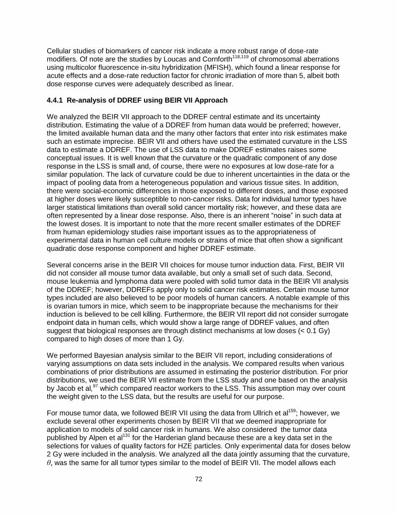
72

Cellular studies of biomarkers of cancer risk indicate a more robust range of dose-rate modifiers. Of note are the studies by Loucas and Cornforth118,119 of chromosomal aberrations using multicolor fluorescence in-situ hybridization (MFISH), which found a linear response for acute effects and a dose-rate reduction factor for chronic irradiation of more than 5, albeit both dose response curves were adequately described as linear. 4.4.1 Re-analysis of DDREF using BEIR VII Approach We analyzed the BEIR VII approach to the DDREF central estimate and its uncertainty distribution. Estimating the value of a DDREF from human data would be preferred; however, the limited available human data and the many other factors that enter into risk estimates make such an estimate imprecise. BEIR VII and others have used the estimated curvature in the LSS data to estimate a DDREF. The use of LSS data to make DDREF estimates raises some conceptual issues. It is well known that the curvature or the quadratic component of any dose response in the LSS is small and, of course, there were no exposures at low dose-rate for a similar population. The lack of curvature could be due to inherent uncertainties in the data or the impact of pooling data from a heterogeneous population and various tissue sites. In addition, there were social-economic differences in those exposed to different doses, and those exposed at higher doses were likely susceptible to non-cancer risks. Data for individual tumor types have larger statistical limitations than overall solid cancer mortality risk; however, and these data are often represented by a linear dose response. Also, there is an inherent ―noise‖ in such data at the lowest doses. It is important to note that the more recent smaller estimates of the DDREF from human epidemiology studies raise important issues as to the appropriateness of experimental data in human cell culture models or strains of mice that often show a significant quadratic dose response component and higher DDREF estimate. Several concerns arise in the BEIR VII choices for mouse tumor induction data. First, BEIR VII did not consider all mouse tumor data available, but only a small set of such data. Second, mouse leukemia and lymphoma data were pooled with solid tumor data in the BEIR VII analysis of the DDREF; however, DDREFs apply only to solid cancer risk estimates. Certain mouse tumor types included are also believed to be poor models of human cancers. A notable example of this is ovarian tumors in mice, which seem to be inappropriate because the mechanisms for their induction is believed to be cell killing. Furthermore, the BEIR VII report did not consider surrogate endpoint data in human cells, which would show a large range of DDREF values, and often suggest that biological responses are through distinct mechanisms at low doses (< 0.1 Gy) compared to high doses of more than 1 Gy. We performed Bayesian analysis similar to the BEIR VII report, including considerations of varying assumptions on data sets included in the analysis. We compared results when various combinations of prior distributions are assumed in estimating the posterior distribution. For prior distributions, we used the BEIR VII estimate from the LSS study and one based on the analysis by Jacob et al,97 which compared reactor workers to the LSS. This assumption may over count the weight given to the LSS data, but the results are useful for our purpose. For mouse tumor data, we followed BEIR VII using the data from Ullrich et al159; however, we exclude several other experiments chosen by BEIR VII that we deemed inappropriate for application to models of solid cancer risk in humans. We also considered the tumor data published by Alpen et al131 for the Harderian gland because these are a key data set in the selections for values of quality factors for HZE particles. Only experimental data for doses below 2 Gy were included in the analysis. We analyzed all the data jointly assuming that the curvature, θ, was the same for all tumor types similar to the model of BEIR VII. The model allows each

73

type of cancer and type of mouse to have its own baseline cancer risk, linear increase, and

quadratic increase in cancer risk. However θ is estimated instead of the quadratic, β term. We fit

the following model to the tumor risk data:

)2.4()]([ 2

acuteii DxIDDcRisk

where D is the dose, i is an indicator for each type of cancer and mouse and I(Dacute) is the indicator function for acute doses. Note that each type of cancer and mouse has a unique value

for β = αi*θ. The model assumes risks are normally distributed with variances that are

proportional to the reciprocal of the squared standard errors. The DDREF can be estimated as 1

+ θ for the dose range of interest here. For the final likelihood function that we combined for the

posterior estimate, we assumed that the DDREF had a log-normal distribution with mean

ln(1+θ) and error determined using the delta method.

BEIR VII did not utilize the data from the chronically exposed mice from the large Argonne National Lab studies reported by Grahn et al.250 In this study, male and female B6CF1 mice (F1 crosses of resistant C57BL/6 and sensitive BALB/c mouse strains) were exposed at 110+7 days

of age to single fraction (acute), 24 once-weekly or 60 once-weekly doses of -rays or neutrons. To support our Bayesian analysis of the DDREF, we considered the acute and 24 once-weekly data (Table 4.3). We did not consider the 60 once-weekly data since it could also include a dose protraction effect independent of dose-rate effects, such as a possible difference in cancer susceptibility for difference mouse ages. We allowed the chronic data to contribute to the estimation of the linear term in the model. Linear dose response, α values were published for both the acute and chronic data. The data were divided into individual epithelial cancers that included lung, liver, Harderian gland, and glandular/reproductive tumors. The data were further divided by gender and into two intervals of ages, 600-799 days and 800-899. For each cancer type, gender, and age interval, the DDREF can be estimated using the published α values as

follows:

)3.4(chronic

acuteDDREF

If again we assume that the DDREF follows a log-normal distribution, we can estimate the variance of the natural log of the DDREF using the standard errors (SE) as:

)4.4()()()][ln( 22

acute

acute

chronic

chronic SESEDDREFVar

The natural logarithm transformed DDREFs can be aggregated across the different cancer types, genders, and age intervals using the generalized inverse variance method. We estimated the effects of protraction due to the age of the mice in the acute exposure being lower than mice at the end of the 24 week chronic exposure. Since no mouse data over a similar age range was available, we made an estimate of the influence of the dose protraction using the UNSCEAR models for humans by comparing risks for an age of exposure of 20 years to that of 35 years, which approximates the 24 wks of life span in the chronically exposed mice.

74

Using this assumption the DDREF for all sites combined in Table 4.3 would be reduced by a small amount to ~1.94. There are also a large number of cell culture studies using surrogate endpoints for cancer risk that have studied dose-rate effects, including mutation, transformation, and chromosomal aberrations. For example recent studies for dose-rate reduction for HPRT mutations vary from about 3 to 8 in studies by Vivek et al 251 and Nakamura et al252, respectively. As an illustration of how human cell culture cancer biomarker data might alter the Bayesian analysis we chose to considered data for translocations measured in a population of 28 astronauts. Astronaut blood

samples were exposed to low doses of -rays 30, 253 and chromosomal aberrations scored with 3 color FISH (Figure 4.1). Each astronaut in the model had their own estimate for initial translocation prevalence, ci and linear increase with dose, αi . The combined curvature, θ, in the linear quadratic fit for astronaut translocation could be determined as:

)5.4(][ 2DDcRisk ii

The model assumes risk are normally distributed with variances that are proportional to the reciprocal of the squared standard errors. The DDREF can be estimated as 1 + θ for the dose range of interest here. For the final likelihood function that we combined for the posterior estimate, we assumed that the DDREF had a log-normal distribution with mean ln(1+θ) and error determined using the delta method.

4.4.2 Combining the distributions using Bayesian methods

A log-normal distribution was fit using the reported LSS DDREF and confidence intervals. The value of μ was estimated as ln(1.3). The upper 95% confidence limit was used to determine the σ value for the log-normal distribution with μ = ln(1.3) and the cumulative distribution at 2.6 = 0.975. This distribution has error at values below 1 for the DDREF. The log-normal distribution adds slightly more uncertainty at these lower values of DDREF. Each prior distribution and likelihood is assumed to be log-normal. Combining these distributions using a conjugate prior determined by the log-normal distributions results in a posterior with a student’s t-distribution on the log scale shown in Figure 4.2. The range of values based on varying choices of which different distributions are combined was for the central estimate a range from 1.41 to 1.9, while the upper 95% confidence interval has a range from 2.6 to 3.19 under different assumptions.

Table 4.3. DDREF values and log-normal function parameter values estimated from Argonne Lab data for

tumor induction in B6CF1 mice comparing acute to 24 weekly fractions (Grahn et al 250

).

Tissue DDREF 95% CI

All Epithelial 1.66 [1.47, 1.87] 0.507 0.061

Lung 1.54 [1.20, 1.98] 0.432 0.128

Live 1.78 [0.8, 3.96] 0.578 0.407

Harderian Gland 2.37 [1.55, 3.63] 0.864 0.217

Glandular/Reproductive 2.72 [1.79, 4.11] 0.999 0.212

All Sites combined 1.99 [1.52, 2.61] 0.688 0.138

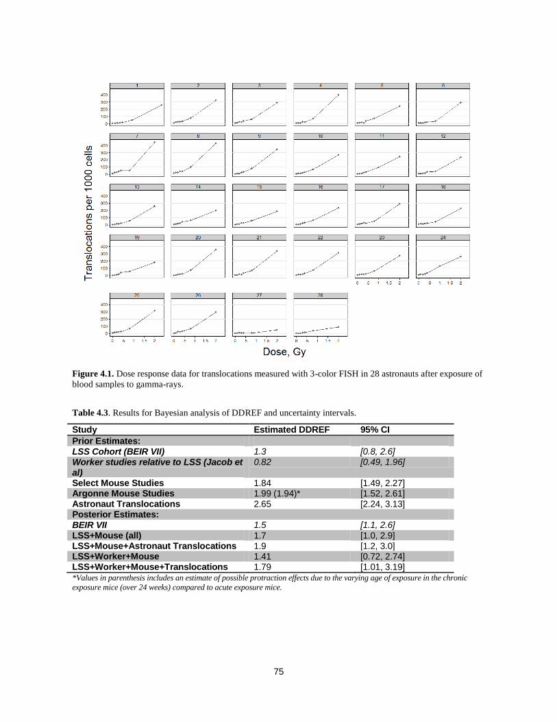
75

Table 4.3. Results for Bayesian analysis of DDREF and uncertainty intervals.

Study Estimated DDREF 95% CI

Prior Estimates: LSS Cohort (BEIR VII) 1.3 [0.8, 2.6] Worker studies relative to LSS (Jacob et al)

0.82 [0.49, 1.96]

Select Mouse Studies 1.84 [1.49, 2.27] Argonne Mouse Studies 1.99 (1.94)* [1.52, 2.61] Astronaut Translocations 2.65 [2.24, 3.13] Posterior Estimates: BEIR VII 1.5 [1.1, 2.6] LSS+Mouse (all) 1.7 [1.0, 2.9] LSS+Mouse+Astronaut Translocations 1.9 [1.2, 3.0] LSS+Worker+Mouse 1.41 [0.72, 2.74] LSS+Worker+Mouse+Translocations 1.79 [1.01, 3.19] *Values in parenthesis includes an estimate of possible protraction effects due to the varying age of exposure in the chronic

exposure mice (over 24 weeks) compared to acute exposure mice.

Figure 4.1. Dose response data for translocations measured with 3-color FISH in 28 astronauts after exposure of

blood samples to gamma-rays.

76

For the NSCR-2012 model, we considered these different estimates of the posterior distribution. Based on the recommendations of the NRC 2012 Committee, we use the BEIR VII central estimate of 1.5. for the DDREF. We used a subjective assessment based on the composite of the different Bayesian results to select the PDF for the DDREF as a Student’s t-distribution with 95% confidence intervals [1, 3.2] as shown in Figure 4.3. One implication of the smaller DDREF is a shift in the overall space radiation uncertainty distribution to be skewed toward higher DDREF values and lower risk although the central estimate is increased.

Figure 4.3. Subjective PDF and CDF representing the DDREF uncertainty in NSCR-2012 model.

DDREF

0.0 0.5 1.0 1.5 2.0 2.5 3.0 3.5 4.0 4.5 5.0

No

rmaliz

ed D

ensity

0.0

0.2

0.4

0.6

0.8

1.0

PDF

CDF

Figure. 4.2. Bayesian posterior probability densities resulting from combining different prior distributions for

DDREF estimates.

77

4.5 Transfer Models Uncertainties

Two models are often considered for transferring radiation-associated incidence or mortality rates from other populations such as the Japanese to a U.S. population. The multiplicative transfer model uses the fitted ERR functions and assumes radiation risks are proportional to spontaneous or background cancer risks. The additive transfer model uses fitted EAR functions to predict cancer risks in the U.S. population and assumes radiation acts independently of other cancer risks. The NCRP recommends6 a mixture model for solid cancers with equal additive contributions from the multiplicative and the additive transfer models. For leukemia risk, the additive transfer model was recommended. There are several considerations with regard to which transfer model is appropriate, least considered of which is the possibility of radiation quality dependence of the transfer model. Additive risk transfer models suggest that radiation acts independently of promotional effects in the population under study. Multiplicative risk transfer models suggest that radiation acts independently of other cancer initiators in the population under study.16 Mouse tumor induction

studies with -rays suggest the multiplicative transfer model is correct for solid cancers and addi-tive transfer for leukemia.121 The transfer model should depend on tissue type if distinct mecha-nisms leading to cancer act in different tissues. There could also be transfer model dependences on age at exposure since older persons compared to younger ones are presumed to have more initiated cells, altered DNA repair capacity, a higher fraction of senescent cells, etc. The transfer model assumption may also depend on radiation quality or become invalid if HZE nuclei and

neutrons produce tumors through different mechanisms than -rays, or on dose if distinct mechanisms of carcinogenesis occur at high vs. low doses.

The possibility to empirically decide on the choice of either multiplicative or additive transfer through inter-comparisons of radiation data from different exposed human populations was discussed by NCRP Report 12615 for stomach, colon, and breast cancers. This analysis suggested stomach cancer was consistent with multiplicative transfer, and results for colon inconclusive. For breast cancer, an additive transfer model is supported but differences in the age at first child birth also needs to be considered.

Lung cancer makes up the highest proportion of the overall cancer risks, and is highly influenced by the use or exposure to tobacco products.254 Thus, it is very important to have accurate transfer model assumptions for the risk of lung cancer. The influence of cigarette smoke on radiation risks for lung and other cancer enters into models in several ways:

1) In background cancer rates, especially important in the application of multiplicative risk models.

2) Competing risks for smokers, former-smokers, and never-smokers.

3) Possible synergistic interactions between smoking and radiation exposure.

Comparisons of radiation lung cancer risks across different cohorts is difficult because of the large influence of primary and secondary tobacco use or exposure in different populations. These inter-comparisons can include comparing the Atomic-bomb survivors to other studies, or comparisons of never-smokers to former or current studies within studies. For example, more than 80% of males and less than 20% of females in the A-bomb survivor study were smokers, but most females were exposed to significant amounts of second-hand smoke. The U.S. Surgeon General’s report 254 estimates an ERR for second-hand smoke of 0.31. The ERR for second-hand smoke is comparable to a gamma-ray lung dose of ~0.4 Sv and is thus a large confounder to deriving risk estimates from epidemiology data. For application at NASA, where most astronauts are never-smokers and the remainder are former-smokers, modeling synergistic

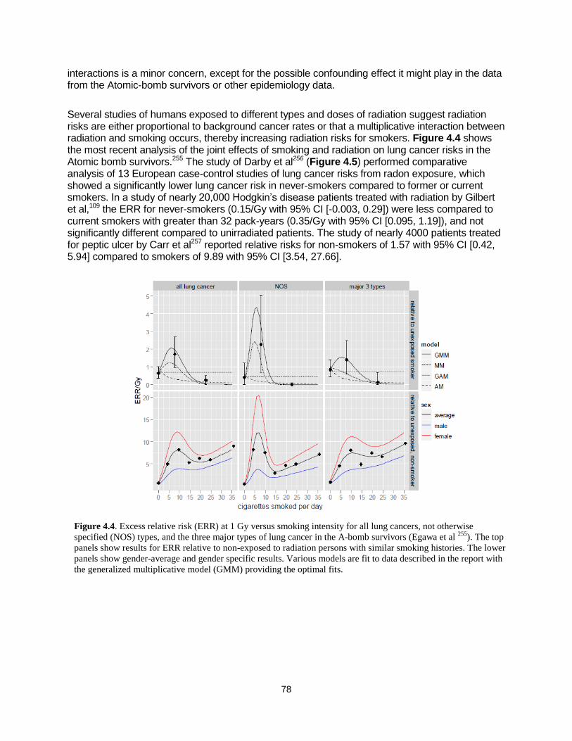
78

interactions is a minor concern, except for the possible confounding effect it might play in the data from the Atomic-bomb survivors or other epidemiology data.

Several studies of humans exposed to different types and doses of radiation suggest radiation risks are either proportional to background cancer rates or that a multiplicative interaction between radiation and smoking occurs, thereby increasing radiation risks for smokers. Figure 4.4 shows the most recent analysis of the joint effects of smoking and radiation on lung cancer risks in the Atomic bomb survivors.255 The study of Darby et al256 (Figure 4.5) performed comparative analysis of 13 European case-control studies of lung cancer risks from radon exposure, which showed a significantly lower lung cancer risk in never-smokers compared to former or current smokers. In a study of nearly 20,000 Hodgkin’s disease patients treated with radiation by Gilbert et al,109 the ERR for never-smokers (0.15/Gy with 95% CI [-0.003, 0.29]) were less compared to current smokers with greater than 32 pack-years (0.35/Gy with 95% CI [0.095, 1.19]), and not significantly different compared to unirradiated patients. The study of nearly 4000 patients treated for peptic ulcer by Carr et al257 reported relative risks for non-smokers of 1.57 with 95% CI [0.42, 5.94] compared to smokers of 9.89 with 95% CI [3.54, 27.66].

Figure 4.4. Excess relative risk (ERR) at 1 Gy versus smoking intensity for all lung cancers, not otherwise

specified (NOS) types, and the three major types of lung cancer in the A-bomb survivors (Egawa et al 255

). The top

panels show results for ERR relative to non-exposed to radiation persons with similar smoking histories. The lower

panels show gender-average and gender specific results. Various models are fit to data described in the report with

the generalized multiplicative model (GMM) providing the optimal fits.

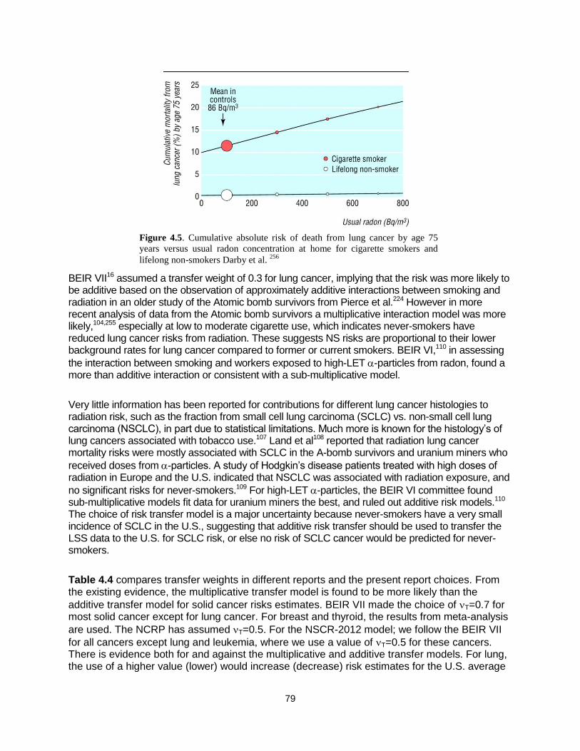
79

BEIR VII16 assumed a transfer weight of 0.3 for lung cancer, implying that the risk was more likely to be additive based on the observation of approximately additive interactions between smoking and radiation in an older study of the Atomic bomb survivors from Pierce et al.224 However in more recent analysis of data from the Atomic bomb survivors a multiplicative interaction model was more likely,104,255 especially at low to moderate cigarette use, which indicates never-smokers have reduced lung cancer risks from radiation. These suggests NS risks are proportional to their lower background rates for lung cancer compared to former or current smokers. BEIR VI,110 in assessing

the interaction between smoking and workers exposed to high-LET -particles from radon, found a more than additive interaction or consistent with a sub-multiplicative model.

Very little information has been reported for contributions for different lung cancer histologies to radiation risk, such as the fraction from small cell lung carcinoma (SCLC) vs. non-small cell lung carcinoma (NSCLC), in part due to statistical limitations. Much more is known for the histology’s of lung cancers associated with tobacco use.107 Land et al108 reported that radiation lung cancer mortality risks were mostly associated with SCLC in the A-bomb survivors and uranium miners who

received doses from -particles. A study of Hodgkin’s disease patients treated with high doses of radiation in Europe and the U.S. indicated that NSCLC was associated with radiation exposure, and

no significant risks for never-smokers.109 For high-LET -particles, the BEIR VI committee found sub-multiplicative models fit data for uranium miners the best, and ruled out additive risk models.110 The choice of risk transfer model is a major uncertainty because never-smokers have a very small incidence of SCLC in the U.S., suggesting that additive risk transfer should be used to transfer the LSS data to the U.S. for SCLC risk, or else no risk of SCLC cancer would be predicted for never-smokers.

Table 4.4 compares transfer weights in different reports and the present report choices. From the existing evidence, the multiplicative transfer model is found to be more likely than the

additive transfer model for solid cancer risks estimates. BEIR VII made the choice of T=0.7 for most solid cancer except for lung cancer. For breast and thyroid, the results from meta-analysis

are used. The NCRP has assumed T=0.5. For the NSCR-2012 model; we follow the BEIR VII

for all cancers except lung and leukemia, where we use a value of T=0.5 for these cancers. There is evidence both for and against the multiplicative and additive transfer models. For lung, the use of a higher value (lower) would increase (decrease) risk estimates for the U.S. average

Figure 4.5. Cumulative absolute risk of death from lung cancer by age 75

years versus usual radon concentration at home for cigarette smokers and

lifelong non-smokers Darby et al. 256

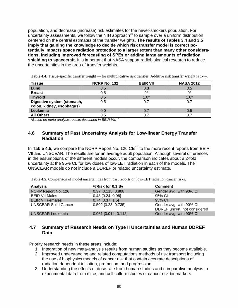
80

population, and decrease (increase) risk estimates for the never-smokers population. For uncertainty assessments, we follow the NIH approach93 to sample over a uniform distribution centered on the central estimates of the transfer weights. The results of Tables 3.4 and 3.5 imply that gaining the knowledge to decide which risk transfer model is correct po-tentially impacts space radiation protection to a larger extent than many other considera-tions, including improved forecasting of SPEs or adding large amounts of radiation shielding to spacecraft. It is important that NASA support radiobiological research to reduce the uncertainties in the area of transfer weights.

4.6 Summary of Past Uncertainty Analysis for Low-linear Energy Transfer Radiation

In Table 4.5, we compare the NCRP Report No. 126 CIs15 to the more recent reports from BEIR VII and UNSCEAR. The results are for an average adult population. Although several differences in the assumptions of the different models occur, the comparison indicates about a 2-fold uncertainty at the 95% CL for low doses of low-LET radiation in each of the models. The UNSCEAR models do not include a DDREF or related uncertainty estimate.

4.7 Summary of Research Needs on Type II Uncertainties and Human DDREF Data

Priority research needs in these areas include:

1. Integration of new meta-analysis results from human studies as they become available. 2. Improved understanding and related computations methods of risk transport including

the use of biophysics models of cancer risk that contain accurate descriptions of radiation dependent initiation, promotion, and progression.

3. Understanding the effects of dose-rate from human studies and comparative analysis to experimental data from mice, and cell culture studies of cancer risk biomarkers.

Table 4.5. Comparison of model uncertainties from past reports on low-LET radiation cancer risks.

Analysis %Risk for 0.1 Sv Comment

NCRP Report No. 126 0.37 [0.115, 0.808] Gender avg. with 90% CI BEIR VII Males 0.48 [0.24, 0.98] 95% CI BEIR VII Females 0.74 [0.37, 1.5] 95% CI UNSCEAR Solid Cancer 0.502 [0.28, 0.735] Gender avg. with 90% CI;

DDREF uncert. not considered UNSCEAR Leukemia 0.061 [0.014, 0.118] Gender avg. with 90% CI

Table 4.4. Tissue-specific transfer weight T for multiplicative risk transfer. Additive risk transfer weight is 1-T.

Tissue NCRP No. 132 BEIR VII NASA 2012

Lung 0.5 0.3 0.5 Breast 0.5 0* 0* Thyroid 0.5 1.0* 1.0* Digestive system (stomach, colon, kidney, esophagus)

0.5 0.7 0.7

Leukemia 0.0 0.7 0.5 All Others 0.5 0.7 0.7 *Based on meta-analysis results described in BEIR VII.

16

81

5. Cancer Risks and Radiation Quality The quality factor (QF) multiplies the absorbed dose to define a dose equivalent for particles

relative to a reference radiation, which is rays.6,25 NASA currently uses the LET, L-dependent radiation QF function, Q(L) that was recommended by the ICRP26 to estimate organ dose equivalents for space missions.6,25,73 Organ doses are evaluated by a mass average of fluence spectra weighted by LET and QFs, Q(L) over each tissue contributing to solid cancer risks. For estimating leukemia risk, organ dose equivalents averaged over bone marrow sites as distributed in adults are used. As described by the NCRP,25 NASA does not use the ICRP radiation weighting factors, which are defined for external fields at the surface of the human body, because of their imprecision and the complex nature of the radiation fields in space. The approach developed at NASA is supported by recommendations by the NCRP in its Report Nos. 1326 and142.25 The ICRP26 definition of the LET-dependent quality function is given by:

>

>

100/300

100102.232.0

/101

)(

LL

L

mkeVL

LQ

The ICRP and NCRP have noted that the use of Q(L) or the alternative radiation weighting factors are simplifications because of lack of knowledge to assign a more precise relationship. QFs are based on a subjective assessment of maximum RBE values, RBEmax for relevant endpoints from radiobiology experimentation. RBEmax is defined as the ratio of initial slopes for the radiation of interest to a reference radiation assuming that both radiation types have linear dose response curves at low dose and dose-rates. It is important to note that it is implicitly as-sumed that DDREFs are not used for particles because RBEmax values are the basis to assign

QFs. The reference radiation should be taken as Cs or Co -rays to accurately represent LSS exposures. RBEs for ions can be underestimated if x rays with energies below about 300 kVp

are used as the reference radiation because the RBE for x rays relative to -rays is greater than unity and observed to exceed 3 at low dose for some endpoints.31 The ICRP and NCRP have noted limitations in radiobiology data to assess radiation QFs.5,31 Other reports have discussed qualitative differences that might preclude the usage of QFs for estimating heavy ion effects.1,5 In this section, we review available radiobiology data for RBEs and discuss biophysical models of radiation quality effects. We will discuss a rationale for defining new radiation quality functions that will:

1) Introduce distinct QFs for solid cancer and leukemia risk estimates.

2) Replace the QF LET dependence with a differential dependence on Z*2/2 for light (Z4) and heavy (Z>4) charged particles.

3) Discuss an alternative risk calculation using track-structure-based risk coefficients. 4) Revise the uncertainty assessment of QFs. 5) Provide an additional uncertainty assessment that considers a nonlinear dose response

at low doses as suggested by NTE models of cancer risk. Uncertainty analysis of radiation quality effects need to address several questions that arise with regard to the radiation quality function including:

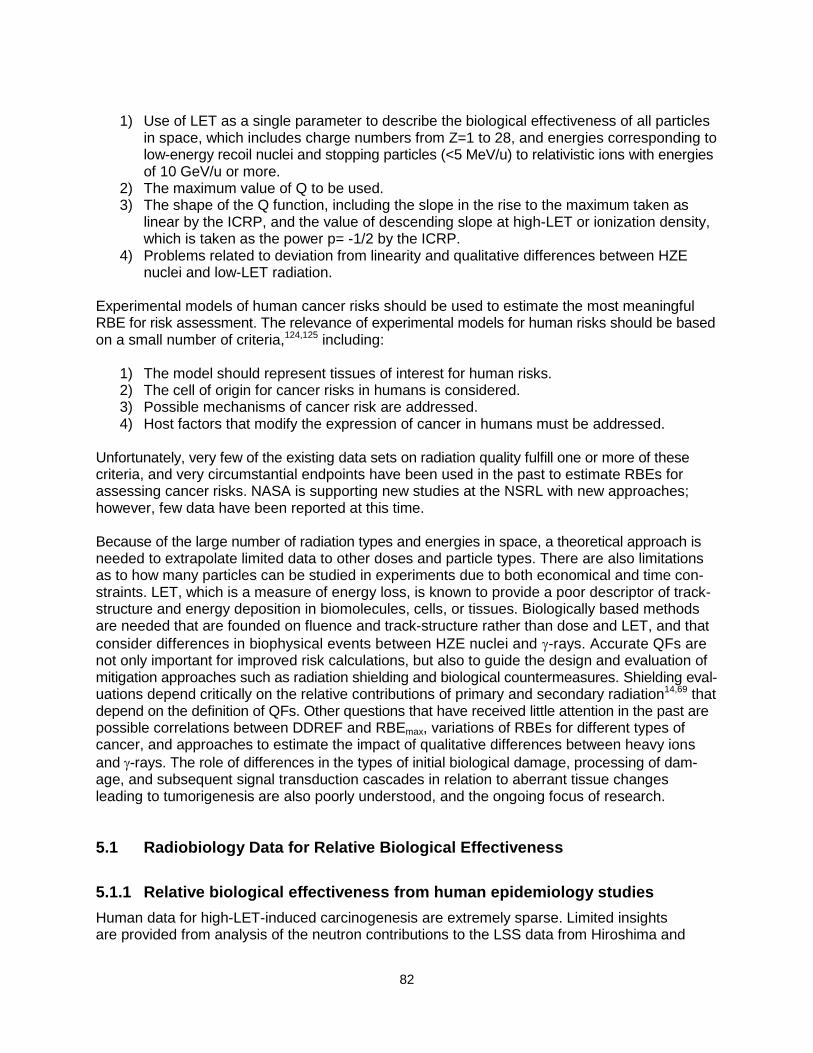
82

1) Use of LET as a single parameter to describe the biological effectiveness of all particles

in space, which includes charge numbers from Z=1 to 28, and energies corresponding to low-energy recoil nuclei and stopping particles (<5 MeV/u) to relativistic ions with energies of 10 GeV/u or more.

2) The maximum value of Q to be used. 3) The shape of the Q function, including the slope in the rise to the maximum taken as

linear by the ICRP, and the value of descending slope at high-LET or ionization density, which is taken as the power p= -1/2 by the ICRP.

4) Problems related to deviation from linearity and qualitative differences between HZE nuclei and low-LET radiation.

Experimental models of human cancer risks should be used to estimate the most meaningful RBE for risk assessment. The relevance of experimental models for human risks should be based on a small number of criteria,124,125 including:

1) The model should represent tissues of interest for human risks. 2) The cell of origin for cancer risks in humans is considered. 3) Possible mechanisms of cancer risk are addressed. 4) Host factors that modify the expression of cancer in humans must be addressed.

Unfortunately, very few of the existing data sets on radiation quality fulfill one or more of these criteria, and very circumstantial endpoints have been used in the past to estimate RBEs for assessing cancer risks. NASA is supporting new studies at the NSRL with new approaches; however, few data have been reported at this time. Because of the large number of radiation types and energies in space, a theoretical approach is needed to extrapolate limited data to other doses and particle types. There are also limitations as to how many particles can be studied in experiments due to both economical and time con-straints. LET, which is a measure of energy loss, is known to provide a poor descriptor of track-structure and energy deposition in biomolecules, cells, or tissues. Biologically based methods are needed that are founded on fluence and track-structure rather than dose and LET, and that

consider differences in biophysical events between HZE nuclei and -rays. Accurate QFs are not only important for improved risk calculations, but also to guide the design and evaluation of mitigation approaches such as radiation shielding and biological countermeasures. Shielding eval-uations depend critically on the relative contributions of primary and secondary radiation14,69 that depend on the definition of QFs. Other questions that have received little attention in the past are possible correlations between DDREF and RBEmax, variations of RBEs for different types of cancer, and approaches to estimate the impact of qualitative differences between heavy ions

and -rays. The role of differences in the types of initial biological damage, processing of dam-age, and subsequent signal transduction cascades in relation to aberrant tissue changes leading to tumorigenesis are also poorly understood, and the ongoing focus of research.

5.1 Radiobiology Data for Relative Biological Effectiveness

5.1.1 Relative biological effectiveness from human epidemiology studies

Human data for high-LET-induced carcinogenesis are extremely sparse. Limited insights are provided from analysis of the neutron contributions to the LSS data from Hiroshima and

83

Nagasaki, or from radon daughter exposures to miners and medical patients exposed to α-emitters. Beyond statistical limitations in such data, there are important differences in the dose distribution among tissues and track-structure between the protons, helium, and HZE nuclei in

space, and low-energy (<10-MeV) neutrons and -particles in terrestrial high-LET exposures. The neutron contributions to the A-bomb survivors’ data are usually treated with an RBE of 10; however, alternative approaches suggest higher dose-dependent values are plausible.113,115 The

BEIR VI report110 made a thorough examination of -particle risks of lung cancer. However, the local deposition of the dose in the lung from radon is quite different from the low-energy helium ions that are produced largely by high-energy GCR protons in all tissues, thus making any infer-ences from these data for space radiation risks quite difficult. ICRP Publication 9231 noted that

studies with -emitters have estimated a low RBE compared to human studies for leukemia with

-rays and x rays. Boice126 estimates, from a study of 1003 patients exposed to thorostrast re-

sulting in -particle exposure to the bone marrow, an effectiveness of -particles 1.33 times

greater than that of -rays in the LSS of A-bomb survivors. In contrast, analysis of studies of liver cancer in thorostrast patients suggests RBEs of about 20 relative to the LSS results.127 These estimates carry large uncertainties. For space radiation, the only epidemiology study reported was the increased risk of cataracts found at low doses (<100 mSv),7,8 which suggests a large RBE (>10) for this endpoint.

5.1.2 Animal carcinogenesis studies with heavy ions

Animal studies generally demonstrate that HZE nuclei have higher carcinogenic effectiveness than low-LET radiation. However, the number of studies of animal carcinogenesis made with HZE nuclei is extremely limited, as summarized in Table 5.1. Dose response studies comparing

tumor induction by -rays or electrons to HZE ions were measured for rat skin,128,129 mouse Harderian gland,130-132 rat mammary gland,133 and mouse leukemia and liver.134 These studies used one or only a few ion types, providing little information on the possible radiation quality dependence on RBE. The exception is the Harderian gland experiments, which consisted of seven particles of differing LET130-132 and other particle exposures in a spread-out Bragg peak.130 Figure 5.1 shows that a similar dose response for solid tumor induction is observed for high-energy Fe nuclei in different murine models at low doses with an absolute excess risk of approximately 25% at 0.2 Gy. Differences in cell sterilization effects or competing risks in the different models lead to different responses at higher doses. No data have been reported for murine models of lung, colon, and several other tumor types important for human radiation risk assessments.

Table 5.1. Tumor induction studies with HZE nuclei.

Tumor Model Tumor type HZE type Reference

Mice (B6CF1) Life-shortening C, Ar, Fe Ainsworth et al135

Mice (B6CF1) Harderian Gland He, C, Ar, Fe Fry et al

130

Mice (B6CF1) Harderian Gland p, He, Ne, Fe, Nb, La Alpen et al132,133

Rat (Sprague-Dawley) Skin tumors Ne, Ar, Fe Burns et al

136.137

Rat (Sprague-Dawley) Mammary tumors Fe Dicello et al133

Mice (CBA) Leukemia, Liver Fe Weil et al

134

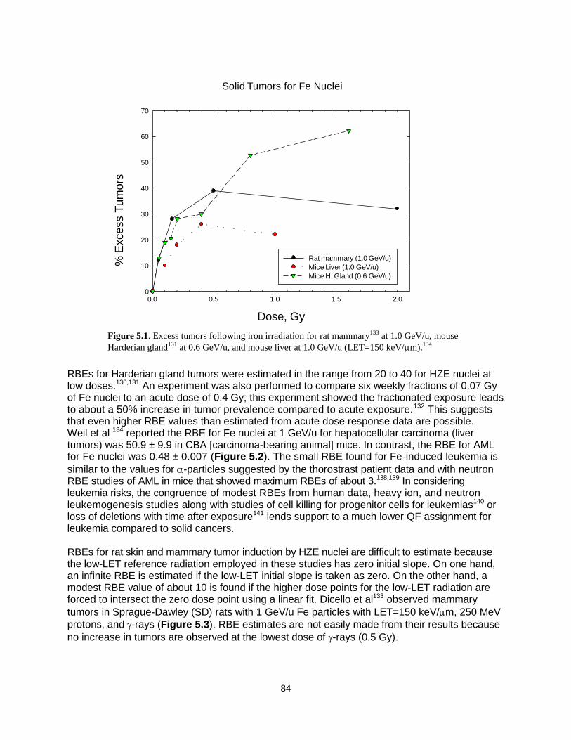
84

RBEs for Harderian gland tumors were estimated in the range from 20 to 40 for HZE nuclei at low doses.130,131 An experiment was also performed to compare six weekly fractions of 0.07 Gy of Fe nuclei to an acute dose of 0.4 Gy; this experiment showed the fractionated exposure leads to about a 50% increase in tumor prevalence compared to acute exposure.132 This suggests that even higher RBE values than estimated from acute dose response data are possible. Weil et al 134 reported the RBE for Fe nuclei at 1 GeV/u for hepatocellular carcinoma (liver tumors) was 50.9 ± 9.9 in CBA [carcinoma-bearing animal] mice. In contrast, the RBE for AML for Fe nuclei was 0.48 ± 0.007 (Figure 5.2). The small RBE found for Fe-induced leukemia is

similar to the values for -particles suggested by the thorostrast patient data and with neutron RBE studies of AML in mice that showed maximum RBEs of about 3.138,139 In considering leukemia risks, the congruence of modest RBEs from human data, heavy ion, and neutron leukemogenesis studies along with studies of cell killing for progenitor cells for leukemias140 or loss of deletions with time after exposure141 lends support to a much lower QF assignment for leukemia compared to solid cancers. RBEs for rat skin and mammary tumor induction by HZE nuclei are difficult to estimate because the low-LET reference radiation employed in these studies has zero initial slope. On one hand, an infinite RBE is estimated if the low-LET initial slope is taken as zero. On the other hand, a modest RBE value of about 10 is found if the higher dose points for the low-LET radiation are forced to intersect the zero dose point using a linear fit. Dicello et al133 observed mammary

tumors in Sprague-Dawley (SD) rats with 1 GeV/u Fe particles with LET=150 keV/m, 250 MeV

protons, and -rays (Figure 5.3). RBE estimates are not easily made from their results because

no increase in tumors are observed at the lowest dose of -rays (0.5 Gy).

Figure 5.1. Excess tumors following iron irradiation for rat mammary133

at 1.0 GeV/u, mouse

Harderian gland131

at 0.6 GeV/u, and mouse liver at 1.0 GeV/u (LET=150 keV/m).134

Solid Tumors for Fe Nuclei

Dose, Gy

0.0 0.5 1.0 1.5 2.0

% E

xcess T

um

ors

0

10

20

30

40

50

60

70

Rat mammary (1.0 GeV/u)

Mice Liver (1.0 GeV/u)

Mice H. Gland (0.6 GeV/u)

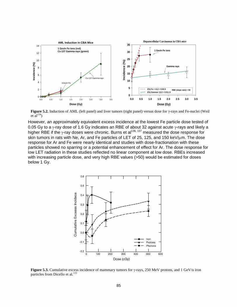
85

However, an approximately equivalent excess incidence at the lowest Fe particle dose tested of

0.05 Gy to a-ray dose of 1.6 Gy indicates an RBE of about 32 against acute -rays and likely a

higher RBE if the -ray doses were chronic. Burns et al136, 137 measured the dose response for

skin tumors in rats with Ne, Ar, and Fe particles of LET of 25, 125, and 150 keV/m. The dose response for Ar and Fe were nearly identical and studies with dose-fractionation with these particles showed no sparring or a potential enhancement of effect for Ar. The dose response for low LET radiation in these studies reflected no linear component at low dose. RBEs increased with increasing particle dose, and very high RBE values (>50) would be estimated for doses below 1 Gy.

Figure 5.3. Cumulative excess incidence of mammary tumors for -rays, 250 MeV protons, and 1 GeV/u iron

particles from Dicello et al.133

Figure 5.2. Induction of AML (left panel) and liver tumors (right panel) versus dose for -rays and Fe-nuclei (Weil

et al134

)

Dose (Gy)

0.0 0.5 1.0 1.5 2.0 2.5 3.0 3.5

Incid

en

ce (

%)

0

2

4

6

8

10

12

14

Cs-137 Gamma-rays

1Gev/n Fe

AML Induction in CBA Mice

1 Gev/n Fe ions (red) Cs-137 Gamma-rays (green)

Dose (Gy)

0.0 0.5 1.0 1.5 2.0 2.5 3.0 3.5

Incid

en

ce (

%)

0

5

10

15

20

25

30

35

Gamma rays

1 Gev/n Fe ions

I(%) Fe = 12.2 + 0.56 D

I(%) Gamma= 12.2 + 0.011 DRBE (slope ratio) = 50

Hepatocellular Carcinomas in CBA mice

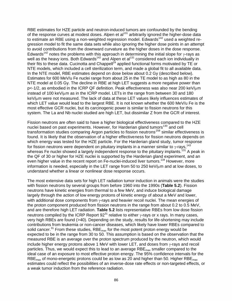
86

RBE estimates for HZE particle and neutron-induced tumors are confounded by the bending of the response curves at modest doses. Alpen et al131 arbitrarily ignored the higher-dose data to estimate an RBE using a non-weighted regression model. Edwards142 used a weighted re-gression model to fit the same data sets while also ignoring the higher dose points in an attempt to avoid contributions from the downward curvature as the higher doses in the dose response.

Edwards142 notes the problems with this approach in determining the initial slope for -rays as well as the heavy ions. Both Edwards142 and Alpen et al131 considered each ion individually in their fits to these data. Cucinotta and Chappell24 applied functional forms motivated by TE or NTE models, which included a cell sterilization term, and made a global fit to all available data. In the NTE model, RBE estimates depend on dose below about 0.2 Gy (described below). Estimates for 600 MeV/u Fe nuclei range from about 25 in the TE model to as high as 80 in the NTE model at 0.05 Gy. The decline in RBE at high LET suggests a more negative power than

p<-1/2, as embodied in the ICRP QF definition. Peak effectiveness was also near 200 keV/m

instead of 100 keV/m as in the ICRP model. LETs in the range from between 30 and 180

keV/m were not measured. The lack of data at these LET values likely influences estimates of which LET value would lead to the largest RBE. It is not known whether the 600 MeV/u Fe is the most effective GCR nuclei, but its carcinogenic power is similar to fission neutrons for this system. The La and Nb nuclei studied are high LET, but dissimilar Z from the GCR of interest. Fission neutrons are often said to have a higher biological effectiveness compared to the HZE nuclei based on past experiments. However, for Harderian gland tumors130 and cell transformation studies comparing Argon particles to fission neutrons258 similar effectiveness is found. It is likely that the observation of a higher effectiveness for fission neutrons depends on which energy was tested for the HZE particle. For the Harderian gland study, tumor response

for fission neutrons were dependent on pituitary implants in a manner similar to -rays,143 whereas Fe nuclei showed a largely independent response to the pituitary implants.131 A peak in the QF of 30 or higher for HZE nuclei is supported by the Harderian gland experiment, and an even higher value in the recent report on Fe-nuclei-induced liver tumors.134 However, more

information is needed, especially in the LET range from 50 to 250 keV/m and at low doses, to understand whether a linear or nonlinear dose response occurs.

The most extensive data sets for high LET radiation tumor induction in animals were the studies with fission neutrons by several groups from before 1960 into the 1990s (Table 5.2). Fission neutrons have kinetic energies from thermal to a few MeV, and induce biological damage largely through the action of low energy protons of kinetic energy of about a MeV and lower,

with additional dose components from -rays and heavier recoil nuclei. The mean energies of the proton component produced from fission neutrons in the range from about 0.2 to 0.5 MeV, and are therefore high LET radiation. Table 5.2 lists representative RBEs from low dose fission

neutrons compiled by the ICRP Report 9231 relative to either -rays or x rays. In many cases, very high RBEs are found (>40). Depending on the study, results for life-shortening may include contributions from leukemia or non-cancer diseases, which likely have lower RBEs compared to solid cancer.31 From these studies, RBEmax for the most potent proton energy would be expected to be in the range from 30 to 50. This assumption is based on the observation that the measured RBE is an average over the proton spectrum produced by the neutron, which would

include higher energy protons above 1 MeV with lower LET, and doses from -rays and recoil particles. Thus, we would expect this to lead to an average RBEmax smaller compared to the ideal case of an exposure to most effective proton energy. The 95% confidence intervals for the RBEmax of mono-energetic protons could be as low as 20 and higher than 50. Higher RBEmax estimates could reflect the possibilities of an inverse-dose rate effects or non-targeted effects, or a weak tumor induction from the reference radiation.

87

In contrast to low energy protons (< 1 MeV), RBE studies for tumors induced by high-energy protons in animals are generally close to 1, with reports lower than 1,265 and as high as 2.131 The higher values could reflect the secondary target fragments produced by the protons in tissue, which could have much higher LET compared to the primary particle. In the NASA approach to risk assessment, the contributions from secondaries produced in tissue are counted separately from the primary particle using radiation transport models and the additivity assumption applied at low dose and dose-rate. Thus, when considering radiobiological data for high-energy protons (and neutrons), a careful assessment of the secondary radiation in tissue is made.

5.1.3 Cellular studies on chromosomal aberrations and mutation

Because of their smaller costs, cellular studies for endpoint presumed to be involved in cancer risks have been used more extensively compare to animal studies for the purpose of understanding radiation quality effects. These studies show that for a large majority of biological

endpoints, RBE peaks around 100 to 200 keV/m, and then decreases at higher LET values. HZE nuclei are very effective at producing chromosomal exchanges with RBE values exceeding 30 in interphase (as visualized using premature chromosome condensation)144 and 10 at the first post-irradiation mitosis for HZE nuclei.145 Table 5.3 shows RBEmax for chromosomal aberrations (CA) human lymphocytes estimates for several energies of Si, Ti, and Fe nuclei. Figure 5.4 compares Si and Fe data to data for neoplastic transformation of mouse C3H10T1/2 cells.146 A sharp peak in the RBE curve appears at specific LET values similar to those of the ICRP model. However, through use of more energies in the CA study, the LET value in which the peak occurs is shown to increase with increasing Z. Individual curves for each Z are not observed if LET is varied with limited E resolution. A smaller RBEmax is found for the transformation experiments because the RBEs are based on acute dose of 225-kVp x rays

not -rays, and are the RBEs at 50% cell survival levels, which lead to smaller values of RBEmax

compared to low doses (eg, higher survival levels) of -rays.

Table 5.2. Estimates of RBEs for life-shortening and tumors for fission neutrons.

Model Endpoint RBEmax Reference B6CF1 mice (F) Life-shortening 43+6 Carnes et al

259

B6CF1 mice (M) Life-shortening 24+4 “”

B6CF1 mice (M) Life-shortening 42+7 “”

Several mouse strains

With 0.7 MeV average

neutron energy

Life-Shortening 11 to 30 Neary et al260

CBA/CNE mice (M) Life-Shortening 24 to 47 (X-rays) Dimajo et al261

CBA/CNE mice (F) Life-Shortening 7 to 9 (X-rays) “””

SD rats Life-Shortening 35 (1 Gy Gamma) Wolf et al262

Tumors:

BALB/c mice (F) Lung tumors 20 (12 to 30) Ullrich et al159

BALB/c mice (F) Mammary tumors 27 (13 to 41) “”

B6CF1 mice (M) Lung 25 + 4 Grahn et al250

B6CF1 mice (M) All Epithelial tumors 26 + 4 “”

B6CF1 mice (M) Vascular tumors 15 + 3 “”

SD rats (M) Lethal Tumors >50 Wolf et al262

SD rats (M) Lung tumors >50 Lafuma et al263

SD rats (F) Mammary tumors >50 Shellabarger et al264

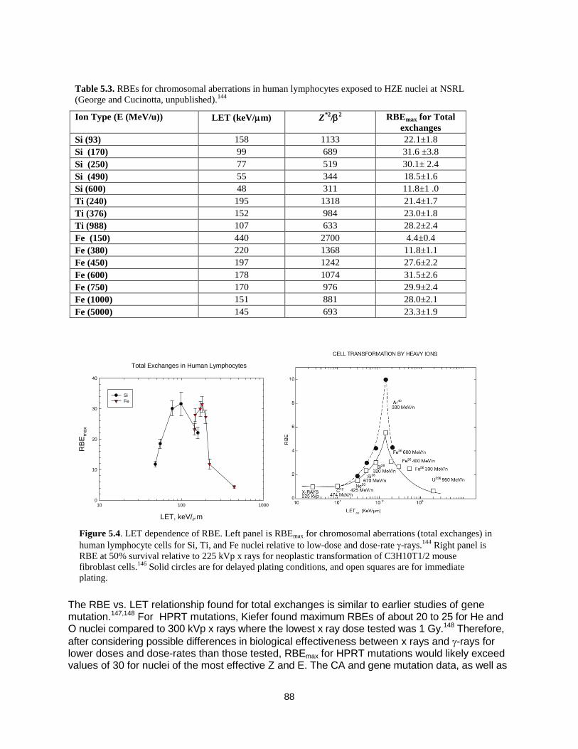
88

The RBE vs. LET relationship found for total exchanges is similar to earlier studies of gene mutation.147,148 For HPRT mutations, Kiefer found maximum RBEs of about 20 to 25 for He and O nuclei compared to 300 kVp x rays where the lowest x ray dose tested was 1 Gy.148 Therefore,

after considering possible differences in biological effectiveness between x rays and -rays for lower doses and dose-rates than those tested, RBEmax for HPRT mutations would likely exceed values of 30 for nuclei of the most effective Z and E. The CA and gene mutation data, as well as

Figure 5.4. LET dependence of RBE. Left panel is RBEmax for chromosomal aberrations (total exchanges) in

human lymphocyte cells for Si, Ti, and Fe nuclei relative to low-dose and dose-rate -rays.144

Right panel is

RBE at 50% survival relative to 225 kVp x rays for neoplastic transformation of C3H10T1/2 mouse

fibroblast cells.146

Solid circles are for delayed plating conditions, and open squares are for immediate

plating.

Total Exchanges in Human Lymphocytes

LET, keV/ m

10 100 1000

RB

Em

ax

0

10

20

30

40

Si

Fe

Table 5.3. RBEs for chromosomal aberrations in human lymphocytes exposed to HZE nuclei at NSRL

(George and Cucinotta, unpublished).144

Ion Type (E (MeV/u)) LET (keV/m) Z*2

/2 RBEmax for Total

exchanges

Si (93) 158 1133 22.1±1.8

Si (170) 99 689 31.6 ±3.8

Si (250) 77 519 30.1± 2.4

Si (490) 55 344 18.5±1.6

Si (600) 48 311 11.8±1 .0

Ti (240) 195 1318 21.4±1.7

Ti (376) 152 984 23.0±1.8

Ti (988) 107 633 28.2±2.4

Fe (150) 440 2700 4.4±0.4

Fe (380) 220 1368 11.8±1.1

Fe (450) 197 1242 27.6±2.2

Fe (600) 178 1074 31.5±2.6

Fe (750) 170 976 29.9±2.4

Fe (1000) 151 881 28.0±2.1

Fe (5000) 145 693 23.3±1.9

89

other data for cell inactivation, imply a larger RBE at the peak for lower Z and fixed values of LET, which is consistent with the predictions of track-structure models. These data also suggest the slope, p, of the falloff with LET on the low-energy side of the RBE peak is more negative than in the ICRP Q. On the high-energy side of the peak, the RBE appears to decline in a manner underrepresented by LET. Here, the LET is nearly constant at these energies as nuclei approach or exceed minimum ionization (~2 GeV/u). A single experimental campaign was made at the Brookhaven National Laboratory (BNL) alternating gradient synchrotron (AGS) using ions of 5 GeV/u, allowing for a comparison to results for Fe from NSRL or other facilities. George and Cucinotta144 compared CAs for Fe at 0.6, 1, and 5 GeV/u with LEs of 178, 150, and 145

keV/m. Results suggest the decline in RBE with increasing E was greater than a LET dependence would predict. In fact, the ICRP Q(LET) model estimates an increased effectiveness for Fe nuclei as the energy is increased above 600 MeV/u. Track structure models that take into account the broadening of a track as velocity is increased predict RBE declines as energy is increased above 600 MeV/u.149

5.2 Qualitative Differences of HZE Particles with Low LET Radiation A growing number of studies report qualitative differences observed in radiobiology experiments when comparing HZE particles and other high LET radiation to low LET radiation. These observations originate from the much higher and distinct patterns of energy deposition in biomolecules, cells and tissues – ie, track structure – for HZE particles, as described below. Distinct contributions from various reactive oxygen species and their clustering along the particle track in cells and tissues also occurs, which are described below. HZE particles and other high LET radiation cause increased clustering of DNA damage leading to more complex DSB’s and other complex DNA damage types,163,266,267 and which leads inhibition of the non-homologous end-joining (NHEJ) repair pathway268,269 or higher levels of residual DNA damages.270-272 The patterns of DSB foci are qualitatively different for HZE particles,2,273,274 and cell cycle differences occur as revealed using flow cytometry.272 Differences between the kinetics of loss of DNA repair foci measured in two-dimensional versus three-dimensional cell cultures are observed comparing HZE particles to low LET radiation. These differences are suggestive of qualitative differences.275 New imaging techniques are being developed to observe repair foci in vivo276 and could be applied to HZE particle irradiation and other radiation types. The quality of chromosome damage or the mutation spectra has been noted to be different when heavy ions are compared to sparsely ionizing radiation.147 Novel multicolor fluorescence

painting techniques of human chromosomes have clearly demonstrated that -particles and iron ions induce many more complex-type chromosomal exchanges in human cells than low-LET radi-ation.150,151 Most of these complex chromosomal rearrangements will ultimately lead to cell death. In fact, only a small fraction of the initial damage is transmitted in mice 2 to 4 months after expo-sure to energetic Fe ions. A low RBE for induction of late chromosomal damage was observed in the progeny of human lymphocytes exposed in vitro to energetic Fe particle, with the interesting exception of terminal deletions; this occurred with much higher frequency with heavy

ions compared to -rays, leading to a very large RBE value.152 Qualitative differences related to telomere dysfunction have been report for Fe particles.277

Qualitative differences in gene expression278-281 between high and low LET, high and low dose, and tissue type have been studied (Figure 5.5) and provide insights into differences in

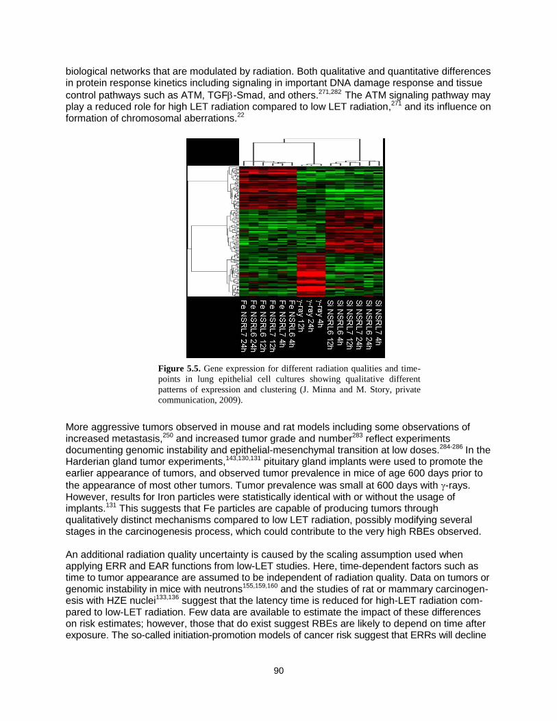
90

biological networks that are modulated by radiation. Both qualitative and quantitative differences in protein response kinetics including signaling in important DNA damage response and tissue

control pathways such as ATM, TGF-Smad, and others.271,282 The ATM signaling pathway may play a reduced role for high LET radiation compared to low LET radiation,271 and its influence on formation of chromosomal aberrations.22

More aggressive tumors observed in mouse and rat models including some observations of increased metastasis,250 and increased tumor grade and number283 reflect experiments documenting genomic instability and epithelial-mesenchymal transition at low doses.284-286

In the Harderian gland tumor experiments,143,130,131 pituitary gland implants were used to promote the earlier appearance of tumors, and observed tumor prevalence in mice of age 600 days prior to

the appearance of most other tumors. Tumor prevalence was small at 600 days with -rays. However, results for Iron particles were statistically identical with or without the usage of implants.131 This suggests that Fe particles are capable of producing tumors through qualitatively distinct mechanisms compared to low LET radiation, possibly modifying several stages in the carcinogenesis process, which could contribute to the very high RBEs observed.

An additional radiation quality uncertainty is caused by the scaling assumption used when applying ERR and EAR functions from low-LET studies. Here, time-dependent factors such as time to tumor appearance are assumed to be independent of radiation quality. Data on tumors or genomic instability in mice with neutrons155,159,160 and the studies of rat or mammary carcinogen-esis with HZE nuclei133,136 suggest that the latency time is reduced for high-LET radiation com-pared to low-LET radiation. Few data are available to estimate the impact of these differences on risk estimates; however, those that do exist suggest RBEs are likely to depend on time after exposure. The so-called initiation-promotion models of cancer risk suggest that ERRs will decline

Figure 5.5. Gene expression for different radiation qualities and time-

points in lung epithelial cell cultures showing qualitative different

patterns of expression and clustering (J. Minna and M. Story, private

communication, 2009).

91

with time after exposure16 and RBEs that depend on time after exposure are predicted from these models.161

Genomic instability in the form of delayed chromosomal aberrations or micronuclei has been measured in mice or rats by several groups,153-156,287 two-dimensional cell culture models,157 and more recently three-dimensional cell culture models have also been studied for genomic insta-bility.158,288 These studies are typically undertaken to understand mechanisms and verify effects, and are often limited by the number of radiation qualities and doses studied. The relationship between delayed micronuclei appearance or chromosomal aberrations and cancer risk is also poorly understood. In general, high-LET radiation is more effective in producing chromosomal instability and delayed micronuclei than low-LET radiation and, in some cases, no effect is ob-served for low-LET radiation. However, RBE or dose-response curves have not been studied in any detail for these endpoints. For proton and HZE nuclei exposures at a low dose-rate of more than a few months, new biological factors may influence risk assessments, including redistribution in the cell cycle, repopulation, or promotional effects, especially when particle fluence is large enough to lead to multiple hits of target cells or surrounding cells and tissue. Very few experimental data are at low dose-rates for HZE nuclei. Burns et al136 found split doses of Ar ions separated by from a few hours up to 1 day increased the risk of skin cancer in rats. Alpen et al132 found using seven 2-week fractions of 0.07 Gy of iron increased risk to 50% compared to a single acute dose of 0.4 Gy for Harderian gland tumors in mice. The Skyhook study of Ainsworth135 considered life shortening in mice, comparing single acute with weekly fractions of several ions; however, the results were unclear with regard to any increase or decrease in risk as dose-rate is decreased.

For -rays and neutrons, a number of studies for cancer induction or life shortening in mice were

made, showing that the sparring effects for -rays and neutron effects may be increased due to protraction under certain conditions in some tissues.159,160 Important questions related to the dif-ferences in life span, cell turnover rates, the role of cell killing, and mechanisms of initiation or promotion in humans and mice make difficult the estimates of the effects of protraction on risk. Elucidating possible differences in inflammation290 and immune responses at high vs. low or chronic doses is also needed to improve risk estimates. If protraction effects do increase the risk from high-LET radiation, such effects would be more important for a Mars mission than for the shorter lunar missions. More recent studies of epigenetic mechanisms are investigating the role of methylation changes and mirco-RNA modifications for irradiation of mice or tissue culture models with HZE particles.290-293 These studies have begun to elucidate possible qualitative differences of GCR with low LET radiation, suggesting differences in epigenetic reprogramming mechanisms. Other studies are detailing micro-RNA controls on ROS responses,294 and the relationship between persistent ROS and mitochondria dysregulation.295

5.3 Biophysical Considerations The term ―track-structure‖ refers to the description of the position of excitations and ionization of target molecules from the passage of ions through DNA, cells, or tissues. It is these initial insults from particles interacting with biomolecules that lead to all biological damage from radiation. Two types of initial damage are considered: DNA damage through direct ionization or oxidative rad-icals; and oxidative damage to non-DNA structures (water molecules, proteins, etc.) leading to changes in signaling or tissue status and function. Track structure descriptions are used in theoretical models of biological responses to understand and extrapolate limited radiobiology

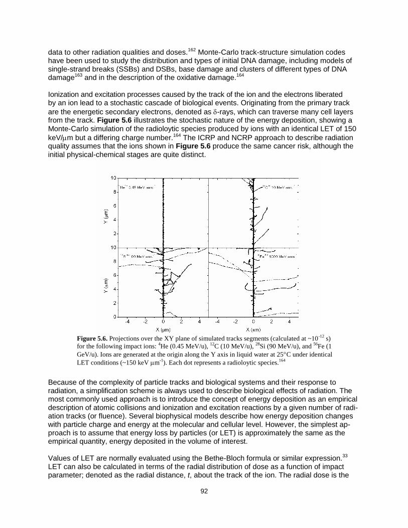
92

data to other radiation qualities and doses.162 Monte-Carlo track-structure simulation codes have been used to study the distribution and types of initial DNA damage, including models of single-strand breaks (SSBs) and DSBs, base damage and clusters of different types of DNA damage163 and in the description of the oxidative damage.164

Ionization and excitation processes caused by the track of the ion and the electrons liberated by an ion lead to a stochastic cascade of biological events. Originating from the primary track

are the energetic secondary electrons, denoted as -rays, which can traverse many cell layers from the track. Figure 5.6 illustrates the stochastic nature of the energy deposition, showing a Monte-Carlo simulation of the radioloytic species produced by ions with an identical LET of 150

keV/m but a differing charge number.164 The ICRP and NCRP approach to describe radiation quality assumes that the ions shown in Figure 5.6 produce the same cancer risk, although the initial physical-chemical stages are quite distinct.

Because of the complexity of particle tracks and biological systems and their response to radiation, a simplification scheme is always used to describe biological effects of radiation. The most commonly used approach is to introduce the concept of energy deposition as an empirical description of atomic collisions and ionization and excitation reactions by a given number of radi-ation tracks (or fluence). Several biophysical models describe how energy deposition changes with particle charge and energy at the molecular and cellular level. However, the simplest ap-proach is to assume that energy loss by particles (or LET) is approximately the same as the empirical quantity, energy deposited in the volume of interest. Values of LET are normally evaluated using the Bethe-Bloch formula or similar expression.33 LET can also be calculated in terms of the radial distribution of dose as a function of impact parameter; denoted as the radial distance, t, about the track of the ion. The radial dose is the

Figure 5.6. Projections over the XY plane of simulated tracks segments (calculated at ~10

-12 s)

for the following impact ions: 4He (0.45 MeV/u),

12C (10 MeV/u),

28Si (90 MeV/u), and

56Fe (1

GeV/u). Ions are generated at the origin along the Y axis in liquid water at 25C under identical

LET conditions (~150 keV m-1

). Each dot represents a radioloytic species.164

93

energy density distribution in a cylindrical shell of radius, t, about the path of the ion.165 Integra-tion of the radial dose distribution over all values of t up to the maximum allowable value, tM, is a measure of the LET:

Mt

exc tDtDtdtLET0

)]()([2 (5.1)

In Eq(5.1), contributions to the radial dose from ionization are denoted as D, and excitations by Dexc. The value of tM, which defines the track width, is a function of particle velocity that corre-sponds to the range of electrons with maximum energy ejected by the passing particle. At suffi-ciently low energies (<0.1 MeV/u), nuclear stopping also contributes to the LET. At very high energy and charge number two-photon emission processes contribute to the LET.166 The track

width can extend well beyond 100 m as the velocity of the ions approaches the speed of light. The primary electron spectrum from ion interactions with target atoms is folded with average transmission properties of electrons to obtain the spatial distribution of electron dose as a function of radial distance from the path of the ion (Kobetich and Katz, 1968):167

dd

dnttE

tdd

ttD

i

i

)],(),([

2

1)( (5.2)

In Eq(5.2) is the initial electron energy, E is the residual energy of an electron with energy

after traveling distance t, and (t,) is the transmission probability that an electron with starting

energy, penetrates a depth, t. Equation (5.2) includes an angular distribution for the number

of primary electrons produced from target atom i, ni, with energy, , and solid angle, . The cross sections for electron production from protons are typically scaled to heavy ions using the effective charge number, Z*, which includes a velocity-dependent screening correction at low energies. The accuracy of the angular distribution is found to substantially modify the radial distribution both at large and small radial distances, and to play only a minor role at intermediate values where a 1/t2 behavior holds. An ansatz168 can be used for the radial dependence of the excitation term, Dexc(t), which is important at small values of t (<10 nm),

2

)2/exp(),,()(

t

dtZACtD excexc

(5.3)

where d=/2 hc/(2r), c is the speed of light, is the ion velocity scaled by c, h is Plank’s

constant, r = 13 eV for water, and Cexc, is a normalization parameter. In Eq(5.3), the radial extension of excitations is confined to very small distances (<10 nm) as characterized by the parameter d.168 Characteristics of the two components of the radial dose are illustrated in Figure

5.7 for nuclei of LET close to 30 keV/m (1 MeV protons and 300 MeV/u Ne).169 The radial dose for Ne extends for many microns, whereas low-energy protons deposit all of their energy within 0.1 micron of the track. The model of Chatterjee et al170 incorrectly assumes that energy deposition in so-called track core and penumbra make equal contributions (50% each); in truth, less than 20% of energy deposition is in the so-called ―core‖ (see reviews by Kraft et al;171 Cucinotta et al169).

94

The frequency distribution of energy imparted to a volume of biomolecular dimensions163 is more closely related to stochastic aspects of radiation tracks described by Monte-Carlo methods than it is to the radial dose. For high-energy ions, frequency distribution can be described using the impact parameter of the ion and distinguishing events in which the ion passes through a vol-

ume (primary-ion or -ray events) and outside a volume (-ray events).172 The two components can be weighted by considering the number of events as a function of impact parameter. The frequency distributions demonstrate energy deposition events in biomolecular targets that occur for high-LET radiation that are not possible with low-LET radiation, even at high doses (up to 100 Gy of low-LET radiation).163 These higher-energy deposition events are usually confined to close to the track of the ion, often called the ―track core,‖ and events similar to low-LET radiation at larger distances, often called the ―track penumbra.‖ The distinction is somewhat arbitrary

because deposition will vary with dimension considered, and because -rays dominate energy deposition in both regions.

Goodhead et al173 reviewed energy deposition models and noted that using the probability of producing >9 ionizations in small volumes (<5 nm diameter), corresponding to a short segment of DNA, provided the best description of increased biological effectiveness at high LET in the experiments of that time. This number of ionizations is related to energy deposition >300 eV in this volume. Microdosimetry approaches, which use micron-size volumes, were shown to be inadequate for describing heavy ion effects or the effects of ultra-soft x rays. Ultra-soft x rays produce only low-energy electrons with short ranges (typically <20 nm), and are a useful probe of mechanisms or radiation action. Ultra-soft x rays were used in several defining experiments to demonstrate failed arguments in microdosimetry-based models. These arguments extend to the use of microdosimetry models of radiation quality, which are often motivated by detector con-siderations rather than radiobiology and are often difficult to interpret due to artifacts such as wall composition, anode wires, and electronic noise inherent in the measurement.

The spatial distribution of -rays plays an important role in describing RBE. Observations by Goodhead et al173 and earlier arguments from Katz,174 predict that biological effects would be

highly influenced by -ray effects rather than by LET alone. Figure 5.8 shows such a description comparing the frequency of energy deposition above 300 eV in a volume the size of the nucleo-

some. The comparisons illustrate that the parameter Z*2/ provides an improved descriptor of

Figure 5.7. Calculations of radial dose distributions to experiments for

1H at 1 MeV (LET=27

keV/m) (left panel) and 20

Ne at 377 MeV/u (LET= 31 keV/m) (right panel).169

t, nm

10-1 100 101 102 103

D(t

), G

y

10-1

100

101

102

103

104

105

106

107

Experiment

Total

Excitations

-rays

t/ nm

10-1 100 101 102 103 104 105 106

D(t

)/ G

y

10-8

10-7

10-6

10-5

10-4

10-3

10-2

10-1

100

101

102

103

104

105

106

Experiments

Total

Excitations

-rays

95

energy deposition in small volumes compared to LET. Deviations from a unique Z*2/ depen-dence occur at low energy where the curves branch for distinct charge numbers. For identical LET values, the ion with the lowest charge is predicted to be more effective at energies above a few MeV/u. Research at the NSRL is making new estimates of radiation quality effects for a variety of endpoints with the focus on approaches to mechanistic understanding of biological effectiveness. However, very few comprehensive studies have been completed at this time. Here we note that, in the past, very detailed studies of radiation quality were made for DNA breaks, as well as for cell inactivation and mutation for a large number of ion types. Such extensive studies would be dif-ficult to repeat today because of the higher costs of many current experimental approaches,

and certainly would take many years to complete. These older studies are useful to consider in terms of track-structure models.

Figure 5.9, from Thacker et al,175 illustrates such track-structure effects for cell inactivation with several ions at a variety of LET values. The upper panel shows the RBE diverging for ions with similar LET values but differing charge numbers, whereas the lower panel shows much

improved convergence when radiation quality is described by the parameter Z*2/. Similar observations by Belli et al176,177 suggested that protons were significantly more damaging than helium at the same LET for V79 cell inactivation and HPRT mutation. More expansive studies of diverging biological effectiveness for particles of identical LET, but differential Z and E, were made with heavy ions with energies from about 1 to 20 MeV/u. Figure 5.10 shows results expressed as an action cross section for inactivation of E. coli Bs-1,178 Bacillus subtilus (rec),179 and V79 mammalian cells.148,175,180 These experiments were compared to the Katz track-structure model by Cucinotta et al,149,181 which is also shown in Figure 5.10. Good agreement is found in comparing the model to experiments. In these comparisons, LET is a poor predictor of biological effectiveness, which was established by the use of many ion types and energies. Track structure models of DNA damage endpoints show similar deviation of LET response for nuclei with different Z. Figure 5.11 shows predictions from Holley and Chatterjee182 for the production of small DNA fragments (0.02 to 20 kbp [kilobase pairs]) by several HZE nuclei. The model shows that for two nuclei with the same LET, the one with the lower Z has a larger

Figure 5.8. Number of nucleosomes per cell receiving 300 eV or more as a function of LET

(left panel) or Z*2

/2 (right panel). Calculations are shown for H, He, Si, and Fe nuclei using

methods of Cucinotta et al.172

10x5 nm (Nucleosome)

LET, keV/m

1 10 100 1000

F(

>300 e

V)

per

Cell,

Gy-1

0

20

40

60

80

100

Proton

Helium

Silicon

Iron

Z*2/

2

1 10 100 1000 10000

96

biological effectiveness. It is also known that the production of the initial oxidative species varies by Z and E, and not by LET alone as shown in Figure 5.11 (right panel). The existing evidence therefore suggests that the radiation quality dependence of both the initial DNA damage and the non-DNA damage, such as the production of various oxidative species, is dependent on Z and LET or alternatively Z and E, and is not well described by LET alone.

Figure 5.10. Cross sections for inactivation of E. coli (panel A), Bacterial spores (panel B), and V79 mammalian

cells (panel C) showing charge number branching in the LET dependence of biological responses (see Cucinotta et

al181

for details).

Figure 5.9. Reproduced from Thacker et al.,175

the relationship between RBE

and ionization density for V79 hamster cells (closed symbols) and T1 human

cells (open symbols). Panel A: RBE vs. LET. Panel B: RBE vs. Z*2

/2.

A B C

97

Although commonly used endpoints (eg, DNA breaks, cell death, mutation, and chromosomal aberrations used to investigate track-structure effects) are limited as surrogate markers to cancer risks, they are used under the assumption that cancer risks would follow similar relative changes as a function of radiation quality. HPRT mutations are clearly related to the deletion of segments of DNA in surviving cells; however, the role of mutations and genomic instability that might evolve from deletions in cancer risk is still debated. While chromosomal aberrations are found in almost all human tumors, they can be both an initiating event or the result of genomic instability from an independent event. The NRC1 recommends that endpoints, such as chromosomal aberrations or cell inactivation, could be studied to evaluate track-structure and shielding effectiveness. However, it would be more useful for track-structure studies to be made with endpoints clearly related to cancer risk.

5.4 Biophysical Models of Relative Biological Effectiveness Dose responses for tumor induction by HZE particles and neutrons often appear to increase linearly at low doses and then bend over at moderate doses of 0.5 Gy or lower due to cell steri-lization effects or competing risks.160 This bending in the dose response makes determination of RBEmax values difficult unless large sample sizes for multiple low doses are used. For describing tumor dose-response data in which cell killing or competing risks modifies the dose response at higher doses, a commonly used functional form, which we denote as the TE model, is given by:

2 ( )

0 [ ( ) ( ) ] L D

TEP P L D L D e (5.4)

where the dose is denoted, D, and P0 is the background tumor probability. The and

coefficients are parameters that will depend on radiation quality. The dose-squared term (with

coefficient ) in Eq(5.4) is normally only considered for -rays or other forms of low-LET radiation

Figure 5.11. Panel A shows calculations of total yields of fragments of double-stranded DNA with sizes from 0.02

to 20 kbp for He, N, and Fe nuclei (for details see Holley and Chatterjee182

) showing that lower Z nuclei have

greater biological effectiveness at identical LET values than higher Z nuclei. Panel B shows results for Laverne183

of ferric ion yields in the Fricke dosimetry illustrating charge branching with LET for oxidative damage effects.

98

such as high-energy protons or helium ions. Equation (5.4) can be thought of as a Taylor series expansion with higher-order terms typically ignored. It is a common assumption to represent radiation quality dependence in terms of LET with the

or linear induction term rising with increasing LET to a peak and then decreasing at higher LET:

0 1 2( ) exp( )L L L (5.5)

And, similarly for the cell sterilization factor:

0 1 2( ) exp( )L L L (5.6)

The Do value for cell killing, which varies by LET, is given by 1/(L). In the TE model, the RBE becomes independent of dose at a sufficiently low dose in which the

cell sterilization term and the -term can be ignored. RBEmax is defined as a low dose-limit given

by the ratio of linear-induction coefficients for -rays and ions:

LTERBE

(5.7)

At low fluence, where less than one particle intersects the biological target under study, the biological action cross section, which is defined as the probability per unit fluence for the end-point considered (eg, cell inactivation, mutation, or tumor induction), is a very useful quantity for discussing particle effects. This concept holds rigorously when exponential or linear dose response curves occur such that the simple relationship applies:

D F (5.8)

Using a conversion factor to have units of m2 for , keV/m for LET, and Gy for dose leads to:

/ 6.24L (5.9)

The RBE is expressed in terms of the linear slope for -rays and the action cross section as:

6.24

RBEL

(5.10)

A complication occurs if the dose response curve for particles contains nonlinear terms. The initial slope in a dose response curve will then be distinct from the final slope or a slope estimated at higher doses. In this case, models of nonlinear terms must be constructed to infer the action

cross section from dose response data.162 The use of fluence is problematic for -rays, because

of the complication of the distribution of electrons of varying LET that mediate -ray effects, and because a ―low electron fluence‖ regime is difficult to observe experimentally for biological endpoints of interest (eg, doses of ~0.01 Gy or less).

99

Because of the large number of particle types and energies in space, parametric representations will be quite limited if no underlying biophysical model is used to describe track-structure and dose response curves. Instead, a parametric approach built on an underlying track-structure model would be very useful for extrapolation of experimental data. Biophysical models can describe how RBEs vary with radiation quality, and can be compared to the assumption of the QF function dependence on LET alone. One consideration is the assumed decline in effec-tiveness at high LET by the power, p=-1/2, in the ICRP definition of Q(L). Katz and Cucinotta184

studied the case in which a multi-target model represents the -ray biological response data. In the Katz model,162 the action cross section is calculated in terms of the radial dose distribution

averaged over the target volume )(tD , and -ray dose response function, P(D), integrating over

all distances from the ions track to the target as:

2 ( ( ))tdtP D t (5.11a)

For ions above about 5 MeV/u with Z<30, the cross section model of Katz et al162 is accurately described by the function:

*2 2/

0 (1 )Z me (5.11b)

where m can be interpreted to represent a target number or hit number, 0 is the saturation area

of the sensitive part of biological system under consideration, and is a measure of the value of

Z*2/2 where approaches 0. These constants are fitted to radiobiological data sets. Equation (5.11) predicts the action cross section above energies of about 5 MeV/u for Z<30, which then

increases with Z*2/2 until reaching a maximum dependent on the value of . If an ion has a charge

and speed such that Z*2/2 > , saturation occurs. Values of ranging from 500 to 2000 were found in fits to a large number of radiobiology experiments with heavy ions.185 The action cross section deviates from this form at lower E where thin-down occurs (narrowing of the track relative

to the biological target size) or for very high Z where >0. At low fluence, the RBE is found to follow the following relationship (Katz and Cucinotta, 1991):184

1/

0

1 1/

m

m

DRBE

F L

(5.12)

where D0 is a radiosensitivity parameter for the -ray data being considered. Equation (5.12)

predicts that the RBE declines once the cross section saturates to its asymptotic value, 0, as higher LET values are reached with a power, p=-1. Katz has also described a ―final slope‖ cross

section for high doses that shows a distinct dependence on Z*2/2 and LET rather than Eq(5.12). At high dose, LET is shown to be a reasonable predictor of radiation quality effects, as should

be expected because here -rays from many overlapping particle tracks occur. Of the biophysical models developed to describe heavy ion effects, the Katz model provides the most robust description of heavy ion dose responses and radiation quality. Mechanistically, the model contains several deficiencies,169,186 including neglect of stochastic aspects of radiation tracks and ignoring differences in biological effectiveness of electrons of different energies. In many applications, the multi-target model is also used, which ignores a linear response term for

-rays and a time-dependent description of damage repair. The idea of an effective target size continues to be debated in radiobiology.187 There appear to be several important dimensions.

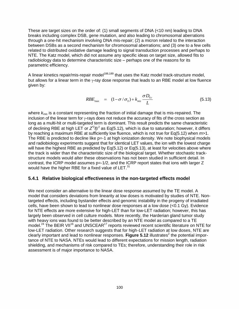
100

These are target sizes on the order of: (1) small segments of DNA (<10 nm) leading to DNA breaks including complex DSB, gene mutation, and also leading to chromosomal aberrations through a one-hit mechanism involving DNA mis-repair; (2) a micron related to the interaction between DSBs as a second mechanism for chromosomal aberrations; and (3) one to a few cells related to distributed oxidative damage leading to signal transduction processes and perhaps to NTE. The Katz model, which did not assume any specific ideas on target size, allowed fits to radiobiology data to determine characteristic size – perhaps one of the reasons for its parametric efficiency. A linear kinetics repair/mis-repair model188,189 that uses the Katz model track-structure model,

but allows for a linear term in the -ray dose response that leads to an RBE model at low fluence given by:

0

max 0(1 / ) mis

DRBE k

L

(5.13)

where kmis is a constant representing the fraction of initial damage that is mis-repaired. The

inclusion of the linear term for -rays does not reduce the accuracy of fits of the cross section as long as a multi-hit or multi-targeted term is dominant. This result predicts the same characteristic

of declining RBE at high LET or Z*2/2 as Eq(5.12), which is due to saturation; however, it differs by reaching a maximum RBE at sufficiently low fluence, which is not true for Eq(5.12) when m>1. The RBE is predicted to decline like p=-1 at high ionization density. We note biophysical models and radiobiology experiments suggest that for identical LET values, the ion with the lowest charge will have the highest RBE as predicted by Eq(5.12) or Eq(5.13), at least for velocities above where the track is wider than the characteristic size of the biological target. Whether stochastic track-structure models would alter these observations has not been studied in sufficient detail. In contrast, the ICRP model assumes p=-1/2, and the ICRP report states that ions with larger Z would have the higher RBE for a fixed value of LET.31

5.4.1 Relative biological effectiveness in the non-targeted effects model

We next consider an alternative to the linear dose response assumed by the TE model. A model that considers deviations from linearity at low doses is motivated by studies of NTE. Non-targeted effects, including bystander effects and genomic instability in the progeny of irradiated cells, have been shown to lead to nonlinear dose responses at a low dose (<0.1 Gy). Evidence for NTE effects are more extensive for high-LET than for low-LET radiation; however, this has largely been observed in cell culture models. More recently, the Harderian gland tumor study with heavy ions was found to be better described by an NTE model as compared to a TE model.24 The BEIR VII16 and UNSCEAR17 reports reviewed recent scientific literature on NTE for low-LET radiation. Other research suggests that for high-LET radiation at low doses, NTE are clearly important and lead to nonlinear responses. Figure 5.12 illustrates2 the potential impor-tance of NTE to NASA. NTEs would lead to different expectations for mission length, radiation shielding, and mechanisms of risk compared to TEs; therefore, understanding their role in risk assessment is of major importance to NASA.

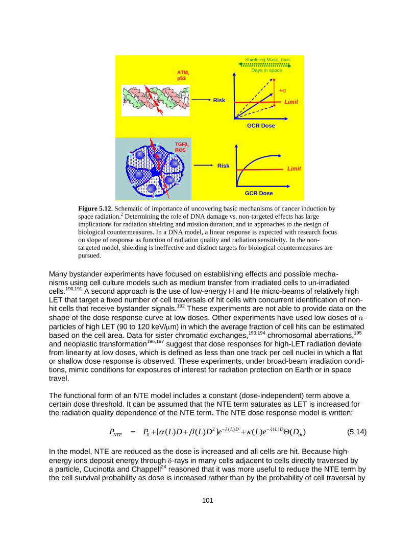
101

Many bystander experiments have focused on establishing effects and possible mecha-nisms using cell culture models such as medium transfer from irradiated cells to un-irradiated cells.190,191 A second approach is the use of low-energy H and He micro-beams of relatively high LET that target a fixed number of cell traversals of hit cells with concurrent identification of non-hit cells that receive bystander signals.192 These experiments are not able to provide data on the

shape of the dose response curve at low doses. Other experiments have used low doses of -

particles of high LET (90 to 120 keV/m) in which the average fraction of cell hits can be estimated based on the cell area. Data for sister chromatid exchanges,193,194 chromosomal aberrations,195 and neoplastic transformation196,197 suggest that dose responses for high-LET radiation deviate from linearity at low doses, which is defined as less than one track per cell nuclei in which a flat or shallow dose response is observed. These experiments, under broad-beam irradiation condi-tions, mimic conditions for exposures of interest for radiation protection on Earth or in space travel. The functional form of an NTE model includes a constant (dose-independent) term above a certain dose threshold. It can be assumed that the NTE term saturates as LET is increased for the radiation quality dependence of the NTE term. The NTE dose response model is written:

2 ( ) ( )

0 [ ( ) ( ) ] ( ) ( )L D L D

NTE thP P L D L D e L e D (5.14)

In the model, NTE are reduced as the dose is increased and all cells are hit. Because high-

energy ions deposit energy through -rays in many cells adjacent to cells directly traversed by a particle, Cucinotta and Chappell24 reasoned that it was more useful to reduce the NTE term by the cell survival probability as dose is increased rather than by the probability of cell traversal by

Figure 5.12. Schematic of importance of uncovering basic mechanisms of cancer induction by

space radiation.2 Determining the role of DNA damage vs. non-targeted effects has large

implications for radiation shielding and mission duration, and in approaches to the design of

biological countermeasures. In a DNA model, a linear response is expected with research focus

on slope of response as function of radiation quality and radiation sensitivity. In the non-

targeted model, shielding is ineffective and distinct targets for biological countermeasures are

pursued.

GCR Dose

Risk

GCR Dose

Risk

Shielding Mass, tons

+

Days in space

Limit

TGF

ROS

Limit

ATM

p53

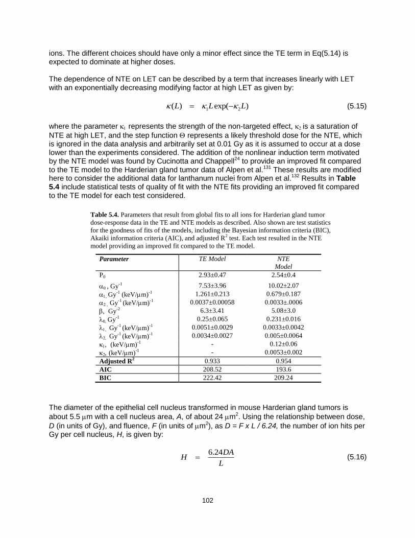
102

ions. The different choices should have only a minor effect since the TE term in Eq(5.14) is expected to dominate at higher doses. The dependence of NTE on LET can be described by a term that increases linearly with LET with an exponentially decreasing modifying factor at high LET as given by:

1 2( ) exp( )L L L (5.15)

where the parameter 1 represents the strength of the non-targeted effect, is a saturation of

NTE at high LET, and the step function represents a likely threshold dose for the NTE, which is ignored in the data analysis and arbitrarily set at 0.01 Gy as it is assumed to occur at a dose lower than the experiments considered. The addition of the nonlinear induction term motivated by the NTE model was found by Cucinotta and Chappell24 to provide an improved fit compared to the TE model to the Harderian gland tumor data of Alpen et al.131 These results are modified here to consider the additional data for lanthanum nuclei from Alpen et al.132 Results in Table 5.4 include statistical tests of quality of fit with the NTE fits providing an improved fit compared to the TE model for each test considered.

The diameter of the epithelial cell nucleus transformed in mouse Harderian gland tumors is

about 5.5 m with a cell nucleus area, A, of about 24 m2. Using the relationship between dose,

D (in units of Gy), and fluence, F (in units of m2), as D = F x L / 6.24, the number of ion hits per Gy per cell nucleus, H, is given by:

6.24DA

HL

(5.16)

Table 5.4. Parameters that result from global fits to all ions for Harderian gland tumor

dose-response data in the TE and NTE models as described. Also shown are test statistics

for the goodness of fits of the models, including the Bayesian information criteria (BIC),

Akaiki information criteria (AIC), and adjusted R2 test. Each test resulted in the NTE

model providing an improved fit compared to the TE model.

Parameter TE Model NTE

Model

P0 2.93±0.47 2.54±0.4

, Gy-1 7.53±3.96 10.02±2.07

1Gy-1

(keV/m)-1

1.261±0.213 0.679±0.187

Gy-1

(keV/m)-1

0.0037±0.00058 0.0033±.0006

Gy-2

6.3±3.41 5.08±3.0

Gy-1

0.25±0.065 0.231±0.016

1 Gy-1

(keV/m)-1

0.0051±0.0029 0.0033±0.0042

Gy-1

(keV/m)-1

0.0034±0.0027 0.005±0.0064

1 (keV/m)-1 - 0.12±0.06

(keV/m)-1 - 0.0053±0.002

Adjusted R2 0.933 0.954

AIC 208.52 193.6

BIC 222.42 209.24

103

Figure 5.13 shows the model fit to the Harderian gland experiment. The comparison shows that less than 1 Fe ion per 100 cells, which is more than double the tumor prevalence. The response curves for the heavy ions display a characteristic change in slope from a low-fluence region, in which NTE effects dominate, to intermediate regions, in which TE dominate and then bend and decrease as cell sterilization contributes at even higher fluence.

The RBE can be estimated near the crossover dose in which the linear induction term is equal to the nontarget term. The crossover dose can be found, for example, from Eq(5.14) as:

( )

( )cr

LD

L

(5.17)

A dose-dependent RBE in then found for the NTE model given for ions of LET, L, at dose, DL by:

( ) ( )

(1 )crNTE TE

L L

DL LRBE RBE

D D

, (5.18)

which is assumed to hold down to a possible threshold dose for the non-targeted effect. The

RBE is thus seen to be dose dependent, even at doses below where cell sterilization and the -term no longer contribute. For chronic irradiation at low fluence as occurs in space, the lower limit or a threshold dose for NTEs becomes an important consideration, and little is known in this regard. Many other considerations need to be addressed including the role of protective NTEs such as the induction of apoptosis, the tissue specificity of NTEs, and temporal aspects.

Figure 5.13. Comparison of NTE2 model24

to experiments131

for prevalence of Harderian

gland tumors vs. the number of radiation tracks per cell nuclei (diameter of 5.5 m). Error

bars represent standard errors. A mean LET of 0.23 keV/m is used to convert dose to

number of radiation tracks for -rays.

Tracks per Cell Nuclei

0.001 0.01 0.1 1 10 100 1000 10000

% P

revale

nce

0

20

40

60-rays (Expt)

H (.4 keV/m)

He (1.6)

Ne (25)

Fe (193)

Fe (253)

Nb (464)

-rays (model)

H (.4 keV/m)

He (1.6)

Ne (25)

Fe (193)

Fe (253)

Nb (464)

104

5.4.2 Saturation mechanisms in biological responses

The declining biological effectiveness at the high ionization density observed in radiobiology experiments can be due to several mechanisms, as described in Table 5.5. The first mechanism is what is termed ―overkill effects,‖ which occur due to energy deposition exceeding a value that is needed to cause an effect. In terms of an action cross section, saturation occurs when the cross section reaches a nearly constant value for increasing ionization densities. A second

mechanism is denoted as ―thindown,‖ which results when the spatial distribution of the -ray brush from an ion becomes limited by kinematics to a size smaller than the biological target size, although the ionization density is still large, often occurring at a velocity at which the Bragg ionization peak occurs. Since thindown depends only on the velocity of the ion and not on Z, it is determined by kinematics. A third mechanism may occur for endpoints such as mutation, neoplas-tic transformation, or perhaps cancer induction when a significant cell killing probability reduces the viability of mutant or carcinogenic cells. Each of these mechanisms needs to be considered when describing the dependence of RBE or QFs with energy and charge as well as dose. A further consideration for cancer data is the role of competing risks from other causes of death, which also may vary with dose and radiation quality.

5.5 Risk Cross Sections and Coefficients Descriptions of radiobiology data in terms of action cross sections lead naturally to the idea of a risk cross section, which originates in the ideas of Katz162,165,198 and is considered by Hoffman et al199 and Curtis et al.200 Such an approach was also discussed in NCRP Report No. 137.201

In this approach, the form for a risk calculation as R = R0 D Q/DDREF is replaced by R = R0

F were denotes a risk cross section. Parametric forms for , as dependent on LET or

Z*2/2 fit to available experimental data or to the ICRP quality function, were considered in NCRP Report No. 137.201 At first glance, it appears that the risk cross section is merely an alternative algebraic representation of the existing calculation replacing dose and Q by fluence and

respectively. What was lacking in NCRP Report No. 137201 was a description of particle track-structure and biophysical considerations on the extrapolation to low dose. We hypothesize that risk cross sections would be useful to NASA if placed in the context of using track-structure and biophysical models to extrapolate experimental observations to other particle types and from acute responses at relatively high doses or fluences to chronic exposures of interest. Another approach was developed by which to consider the neutron components of the Atomic-bomb exposures in Japan. Here, Kellerer and Walsh114 made a direct estimate of a neutron risk coefficient for a typical fission neutron spectrum. Using LSS data to estimate the neutron risk directly avoids the need for the use of the DDREF and its associated uncertainties. The method would not be applicable to space radiation or even other neutron energies, however, because no human data is available to fit a risk coefficient for these radiation types. One idea is that a neutron risk coefficient would represent the maximum value to be expected for any cosmic ray.

Table 5.5. Summary of mechanisms for decline in biological effectiveness at high-energy densities.

Mechanism Impact on RBE Impact on Cross Section,

Overkill RBE declines like 1/LET constant

Thindown RBE declines >1/LET decreases rapidly

Competing risks from cell death or other tumors

Dose dependent decrease at higher doses

does not apply at H>1

H = number of cell hits per particle.

105

However, the uncertainties associated with the neutron risk coefficient – especially with its smaller contribution in the dose estimates from DS02 compared to the earlier DS86 estimates as well as the complex mixture of particles in space – make knowledge of such a maximum estimate of limited value. Estimates of tissue specific neutron risk coefficients would have even larger uncertainties. Furthermore, the space radiation environment is variable, including solar cycle modulation of the GCR energies, random SPE occurrences with variable energies and total fluence, and shielding modifications to the proportion of secondary radiation. Therefore, as in the NCRP Report No. 137 description of a risk cross section, the lack of an underlying track-structure description and dose response model of proton and heavy ion radiobiology limits the applicability of such an approach for describing space radiation risks. Related to the above considerations is the idea to compare proton and HZE particles directly to

high dose-rate -ray data in humans and thereby bypass the need for DDREF estimates and its uncertainties. This approach would be a trade of the DDREF uncertainty and estimates of RBEmax for a model where dose and perhaps dose-rate dependencies of RBEs for particles would need to be estimated. Therefore, re-analysis of the various data sets from the publications described above would be needed to be made for an alternative RBE model replacing RBEmax. We compared the two approaches for the Harderian gland tumor experiment

in Figure 5.14. Using the BEIR VII approach, the DDREF estimate for the Harderian gland -ray data was found as 2.17+1.1. Comparing different approaches, the largest RBE is reduced to

~18 in the model comparing to high dose-rate rays, as compared to ~28 in the model leading to RBEmax in the TE model described above. Therefore, in a model without a DDREF, a scaling factor of 18 would be used. Using the model with a DDREF, a scaling value of 14 is found using a DDREF estimate for the Harderian gland tumor data, whereas a scaling of 21 is found using the BEIR VII DDREF of 1.5. Therefore, the alternative approach falls between possible estimates using a DDREF. However, the uncertainties in the assessment are not likely reduced, and much additional radiobiology data for particles would be needed to implement the approach. We conclude that attempts at a new risk assessment algebra does not necessarily reduce uncertainties and, more importantly, does not alleviate the need to improve the understanding the radiobiology of HZE particles.

Figure 5.14. Comparison of “high dose” model for -ray dose response and RBEs to RBEmax approach. In the left

panel, the dose response for -rays is re-fit using a linear or linear-exponential response model and compared to a

linear-quadratic with exponential response model. The right panel shows the previous result for RBEmax with RBEs

estimated from the “high dose” model for gamma-rays. The lower RBE estimates compared to the estimates of

RBEmax are largely in balance with the estimate of RBE without application of a DDREF.

106

5.6 NASA Radiation Quality Factors

The ideas discussed above on track-structure models and the extrapolation to low dose can be used to allow us to recommend a parametric model for a risk cross section, which is written as188,189:

)),(1(24.6

),(),( 0 EZPLET

EZPEZ

(5.19)

with

mZEZP ))/exp(1(),( 22* (5.20)

where the parameters, 0, m, and should be based on subjective estimates from radiobiology

experiments, and the low-LET slope, , estimated from human epidemiology data for -rays. Using Eqs(5.19) and (5.10), a NASA defined QF function is then written:

),()/(24.6

)),(1(0

EZPLET

EZPQNASA

(5.21)

The interpretation of the parameters is quite general, and is not tied to a particular track-structure models per se, but rather is an efficient parameterization of radiobiology data for

particles. The parameters can be described as follows: 0 is the maximum value of the cross section, which is related to RBEmax for the most biologically effective particle types. m is the slope of the cross section for increasing ionization density, with values m>1 necessary to have

RBE>1. determines the saturation value of the cross section, where the RBE begins to decline. Eq(5.21) provides the central estimate; however, the NASA approach places a higher importance on the overall PDF for QNASA and not the central estimates because of the uncertainties. The overall PDF is estimated by considering possible parameter values that enter into Eq(5.21).

5.6.1. Parameter estimation for NASA quality factors and uncertainties

Estimate of 0 / or Qmax: For solid cancer risks, radiobiology data are sparse. However, the largest RBEmax estimates for HZE nuclei is in the range from 20 to 50 for solid tumors in rodents, and for chromosomal aberrations and mutations in human cells (Figure 5.15). Similarly the largest RBEmax observed for fission neutrons should reflect the values possible for high LET protons with energies below 1 MeV, and fall in the range from 20 to more than 50. Lower value for RBEmax are found for leukemia. These estimates assume a linear dose response at low particle dose, ignoring NTEs or other possible mechanisms, leading to deviation from linearity. Thus, for

example, if a peak RBE value of approximately 40 is assumed for Si at 100 keV/m where

P(Z,E)~1, 0 / can be estimated as 40100/6.24 or described by Qmax=40. Only the ratio, 0

/ is considered here to simplify parameter estimates. The uncertainty distribution of 0 / corresponds to that of the maximum Q value for the most effective particle. Alternative choices for the monoenergetic particle in which the peak occurs would not change numerical estimates appreciably, and calculations should include uncertainty analysis through the use of PDFs to represent subjective assessments of ranges for each parameter. We assume this

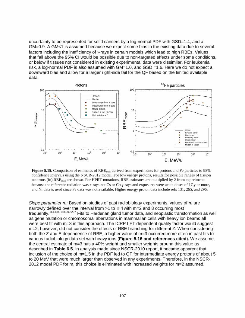
107

uncertainty to be represented for solid cancers by a log-normal PDF with GSD=1.4, and a GM=0.9. A GM<1 is assumed because we expect some bias in the existing data due to several

factors including the inefficiency of -rays in certain models which lead to high RBEs. Values that fall above the 95% CI would be possible due to non-targeted effects under some conditions, or below if tissues not considered in existing experimental data were dissimilar. For leukemia risk, a log-normal PDF is also assumed with GM=1.0, and GSD =1.6. Here we do not expect a downward bias and allow for a larger right-side tail for the QF based on the limited available data.

Slope parameter m: Based on studies of past radiobiology experiments, values of m are

narrowly defined over the interval from >1 to 4 with m=2 and 3 occurring most frequently.161,185,188,209,297 Fits to Harderian gland tumor data, and neoplastic transformation as well as gene mutation or chromosomal aberrations in mammalian cells with heavy ion beams all were best fit with m=3 in this approach. The ICRP LET dependent quality factor would suggest m=2, however, did not consider the effects of RBE branching for different Z. When considering both the Z and E dependence of RBE, a higher value of m=3 occurred more often in past fits to various radiobiology data set with heavy ions (Figure 5.16 and references cited). We assume the central estimate of m=3 has a 40% weight and smaller weights around this value as described in Table 6.5. In analysis made since NSCR-2010 report, it became apparent that inclusion of the choice of m=1.5 in the PDF led to QF for intermediate energy protons of about 5 to 20 MeV that were much larger than observed in any experiments. Therefore, in the NSCR-2012 model PDF for m, this choice is eliminated with increased weights for m=2 assumed.

Figure 5.15. Comparison of estimates of RBEmax derived from experiments for protons and Fe particles to 95%

confidence intervals using the NSCR-2012 model. For low energy protons, results for possible ranges of fission

neutrons (fn) RBEmax are shown. For HPRT mutations, RBE estimates are multiplied by 2 from experiments

because the reference radiation was x rays not Cs or Co -rays and exposures were acute doses of 1Gy or more,

and Ni data is used since Fe data was not available. Higher energy proton data include refs 131, 265, and 296.

Protons

E, MeV/u

10-1 100 101 102 103 104

RB

Em

ax

0.1

1

10

100

95% CI

Median

Lower range from fn data

Upper range from fn data

Mouse tumors

Tumors in rats (Russia)

Hprt Mutation x 2

56Fe particles

E, MeV/u

10-1 100 101 102 103 104

RB

Em

ax

0.1

1

10

100

95% CI

H. Gland tumor

Liver tumor

Mammary tumor

Chrom Aberr.

Hprt Mutation (Ni with Drx2)

Median of Model

108

Track structure parameter : Making an estimate of ranges of possible values of requires

studies of particles of varying E and Z to identify the most effective E or similarly value of Z*2/2 where Qmax occurs. We made estimates based on existing radiobiology experiments for the choice of m=3 and consider other values of m below. Table 5.6 illustrates how E changes for

different Z for fixed values of Z*2/2. The maximum biological effectiveness for protons and He is expected near 0.5 MeV and 1 MeV/u, respectively. Considering Eq(5.21) for m=3, we find the

peak in the quality factor occurs at a value of Z*2/2 =2 . This suggests to ensure the peak in QF

is near a proton energy of 0.5 MeV, requires the value of near 1000. Also the range of allowed

for uncertainty analysis for light particles should be constrained not to be less than =500 or the proton peak RBE would occur above 1 MeV, which is not found in experiments or predicted by track structure models. Data for gene mutation and transformation for He particles overlap

significantly with this choice for . We therefore assumed that values for the parameter below 500 or above 1500 for low Z particles should be excluded.

Figure 5.16. Action cross sections vs. Z*2

/2 for several biological endpoints in mammalian

cells. Experimental data for total exchanges (George and Cucinotta, unpublished),144

dicentrics,202,203

HPRT mutations in human fibroblasts,204,205

human lymphoid cells,206

HPRT

mutations in V79 Chinese hamster cells,148,175,177

and C3H10T1/2 neoplastic

transformation.146,196,207,208

Z*2/

2

10 100 1000

,

m2

0.1

1

10

100

Total Exchanges

Dicentrics

Chromosomal Aberrations in Human Lymphocytes

HPRT Mutations in Human Cells

Z*2

/2

10 100 1000 10000

,

m2

10-5

10-4

10-3

10-2

Fibroblasts

Lymphoid

HPRT Mutations in V79 Cells

Z*2

/2

100 1000 10000

,

m2

10-5

10-4

10-3

10-2

Kiefer expt (Heavy ions)

Thacker or Belli expts

Neoplastic Cell Transformation

Z*2

/2

101 102 103 104 105

,

m2

10-5

10-4

10-3

10-2

10-1

Yang et al. (1993)

Miller el al. (1994)

109

Experiments with Fe nuclei suggest the peak biological effectiveness in the region of kinetic energy of 600 MeV/u, with experiments performed at lower or higher E showing a reduced effectiveness (Figures 5.3 and 5.15). A reasonable range for the RBE peak for Fe is energies of 500 to 1000 MeV/u, which corresponds to Z*2/β2 between 900 and 1300 (see Table 5.6 and Figure 5.17). This implies the value of κ for m=3 would be in the range of κ = 450 and 600. Several studies show the peak for Si to be at about 100 to 300 MeV/u for CA (George and Cucinotta, unpublished),144 gene mutation,206 and neoplastic transformation.146,212 There is a clear reduction in the RBE for Si at 600 MeV/u and higher energies, but less known below 100 MeV/u. The absence of animal tumor data for Si nuclei is an important issue. However, the value of κ based on experiments for Fe particles is largely consistent with the existing data for Si particles. Studies with other particle types, energies and model systems are sparse, and are clearly needed to improve estimates, including studies with O, Ne, Ca, and Ti nuclei.

Because there is little information to make more precise estimates of the value of κ, the approach of the NSCR-2012 models simplifies the calculation of uncertainties to two distributions of particles at each tissue site as a function of Z*2/β2: FLI for Z≤4, and FHI for Z>4. This approach provides flexibility in uncertainty analysis. Future studies can aim to improve descriptions of particle track structure and perhaps consider uncertainty analysis for each charge group. An alternative approach would assume a LET dependent QF function similar to the form used by the ICRP, but with the peak value (currently 100 keV/μm) shifting with increasing Z to higher values. Such an approach would require LET spectra for each Z to be determined, whereas the approach used here allows a simplification into just two spectra for light and heavy particles, and includes considerations of the uncertainty in the rising and falling slope of Q with changing ionization density. The NASA approach has the advantage of simplicity and its relationships to track structure models that consider δ-ray effects.

Figure 5.17. Z*2/β2 versus kinetic energy for several GCR particles. Calculations made using the Barkas formula for effective charger number.

E, MeV/u

10-2 10-1 100 101 102 103 104 105

Z*2 /

β2

10-1

100

101

102

103

104

105

106

107

HHeCOSiCaFe

110

By analysis, we found that the slope, m, is correlated with the position of the maximum value of

Q for varying Z*2/2 as determined by the value of . After studying the functional dependence of the parameters of Eq(5.21), we find that the position of the maximum Q is held fixed for different values of m if the following constraint is used:

04( )

( 1)m

m

(5.22)

where 0 is the estimated value for m=3. In extensive computer analysis, we found that ignoring the condition of Eq(6.7) led to values where the peak value of the QF as kinetic energy is changed for different Z falls outside of what is expected from existing data or basic consideration of track structure models. The uncertainty analysis described below is applied using conditional Monte-Carlo sampling, where a random value of m is selected from its PDF

prior to sampling for the value with central estimate defined by Eq(5.22). This central estimate

of for a given value of m is then allowed to vary with a normal PDF with M=1 and SD=1/3.

Describing radiation quality effects in terms of Z*2/2 is consistent with radial dose models of track-structure, and describes some aspects of stochastic track-structure models. Both LET

and the ionization cross section for -ray production are proportional to Z*2/2; however, LET has

other important Z- and dependent terms at low energy due to atomic shell structure and nuclear

stopping corrections, and at high energies due to the Fermi density effect. The use of Z*2/2 does

not take into account differences in track-width between two particles with identical Z*2/2. This effect will be most important at low energy (<10 MeV/u). Only light ions make important contribu-tions at these energies for GCR because of their longer ranges and the large nuclear production cross sections for hydrogen and helium in tissue. We also assume a description of ―thindown‖ at low energies. Here Eq(5.19) accounts for the saturation, but not for the thindown, mechanism where the track width becomes smaller than the biological target. For low energies, we modify the cross section by the factor PE=1-exp(-E/ETD) to account for thindown. The value of ETD=0.2 is based on experimental data for H and He. This factor has a very small impact for heavy ions since at low E they make a very small contribution for GCR or SPEs. We did not include a PDF describing the possible variation in the ETD parameter since the its influence would overlap with the other parameters in the model such that the model became over-parameterized. Possible deficiencies of radial dose in describing track-structure include the absence of a description of

differences in biological effectiveness of different -rays energies, especially below 10 keV.

Table 5.6. Kinetic energy values for different charge number, Z, corresponding to fixed Z*2/

2. Calculations use the

Barkas model210

of the effective charge number.

Kinetic Energy (MeV/u) for Charge Number (Z) at fixed Z*2

/2

Z*2

/2 1 2 6 10 14 20 26

100 4.7 19.3 234 >10 000 NA NA NA 250 1.85 7.5 75.5 272 1070 NA NA 500 0.93 3.75 35.5 110 264 1155 NA 750 0.61 2.5 23.3 69.4 153 424 2042

1000 0.45 1.85 17.2 50.5 108 272 707 1250 0.35 1.46 13.7 39.8 83.2 199 445 1500 0.28 1.2 11.3 31.6 65.4 157 326 1750 0.24 1.01 9.7 27.8 57.1 130 258 2000 0.2 0.88 8.4 24.2 49.4 110 214

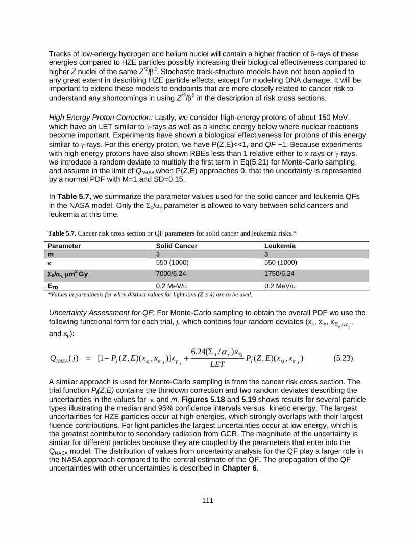
111

Tracks of low-energy hydrogen and helium nuclei will contain a higher fraction of -rays of these energies compared to HZE particles possibly increasing their biological effectiveness compared to

higher Z nuclei of the same Z*2/2. Stochastic track-structure models have not been applied to any great extent in describing HZE particle effects, except for modeling DNA damage. It will be important to extend these models to endpoints that are more closely related to cancer risk to

understand any shortcomings in using Z*2/2 in the description of risk cross sections.

High Energy Proton Correction: Lastly, we consider high-energy protons of about 150 MeV,

which have an LET similar to -rays as well as a kinetic energy below where nuclear reactions become important. Experiments have shown a biological effectiveness for protons of this energy

similar to -rays. For this energy proton, we have P(Z,E)<<1, and QF ~1. Because experiments

with high energy protons have also shown RBEs less than 1 relative either to x rays or -rays, we introduce a random deviate to multiply the first term in Eq(5.21) for Monte-Carlo sampling, and assume in the limit of QNASA when P(Z,E) approaches 0, that the uncertainty is represented by a normal PDF with M=1 and SD=0.15. In Table 5.7, we summarize the parameter values used for the solid cancer and leukemia QFs

in the NASA model. Only the 0/ parameter is allowed to vary between solid cancers and leukemia at this time.

Uncertainty Assessment for QF: For Monte-Carlo sampling to obtain the overall PDF we use the

following functional form for each trial, j, which contains four random deviates (x, xm, x/0,

and xp):

)23.5(),)(,()/(24.6

)],)(,(1[)(0

jmjj

j

jpjmjjNASA xxEZPLET

xxxxEZPjQ

A similar approach is used for Monte-Carlo sampling is from the cancer risk cross section. The trial function Pj(Z,E) contains the thindown correction and two random deviates describing the

uncertainties in the values for and m. Figures 5.18 and 5.19 shows results for several particle types illustrating the median and 95% confidence intervals versus kinetic energy. The largest uncertainties for HZE particles occur at high energies, which strongly overlaps with their largest fluence contributions. For light particles the largest uncertainties occur at low energy, which is the greatest contributor to secondary radiation from GCR. The magnitude of the uncertainty is similar for different particles because they are coupled by the parameters that enter into the QNASA model. The distribution of values from uncertainty analysis for the QF play a larger role in the NASA approach compared to the central estimate of the QF. The propagation of the QF uncertainties with other uncertainties is described in Chapter 6.

Table 5.7. Cancer risk cross section or QF parameters for solid cancer and leukemia risks.*

Parameter Solid Cancer Leukemia

m 3 3

550 (1000) 550 (1000)

0/ m2 Gy 7000/6.24 1750/6.24

ETD 0.2 MeV/u 0.2 MeV/u

*Values in parenthesis for when distinct values for light ions (Z 4) are to be used.

112

Figure 5.18. Results from Monte-Carlo analysis for the overall PDF of the NASA QF function for solid cancers versus kinetic energy for p, He, O, Si, Ca, and Fe

particles. The graphs display the median value and 95% confidence intervals.

Iron

E, MeV/u

10-1 100 101 102 103 104 105

QS

olid

0.1

1

10

100

Median and 95% CI

Calcium

E, MeV/u

10-1 100 101 102 103 104 105

QS

olid

0.1

1

10

100

Median and 95% CI

Oxygen

E, MeV/u

10-1 100 101 102 103 104 105

QS

olid

0.1

1

10

100

Median and 95% CI

Helium

E, MeV/u

10-1 100 101 102 103 104 105

QS

olid

0.1

1

10

100

Median and 95% CI

Protons

E, MeV/u

10-1 100 101 102 103 104 105

QS

olid

0.1

1

10

100

Median and 95% CI

Silicon

E, MeV/u

10-1 100 101 102 103 104 105

QS

olid

0.1

1

10

100

Median and 95% CI

113

Fig. 5.19. Results from Monte-Carlo analysis for the overall PDF of the NASA QF function for leukemia versus kinetic energy for p, and Fe particles. The

graphs display the median value and 95% confidence intervals.

Iron

E, MeV/u

10-1 100 101 102 103 104 105

QLeukem

ia

0.1

1

10

Median and 95% CI

Proton

E, MeV/u

10-1 100 101 102 103 104 105

QLeukem

ia

0.1

1

10

Median and 95% CI

114

5.7 Recommendations for Research Needs on Radiation Quality Future research on radiation quality effects should include:

1. Improving estimates of the maximum QF for several tissues including lung, colorectal, and liver cancers.

2. Assessing the role of NTEs and other mechanisms that could lead to deviation from linear responses. This research should consider chronic radiation with protons and HZE particles

3. Understanding the potential impacts of correlations between DDREF and RBEs from experimental results, and possible variation of experimentally derived values with DDREF’s estimates from human epidemiology data.

4. Determining reliable biomarkers to improve the assessment of the and m parameters in the NASA QF or risk cross section.

5. Improving track structure based biophysics models of radiation quality, including the development of alternative cancer risk models, and systems biology approaches.

6. The NASA QF adequately describes the variation of biological effectiveness based on models of track structure and intra-cellular effects. However, the role of correlations in inter-cellular damage for single HZE particles should be investigated as it relates to RBE in order to understand if increased biological effectiveness might result for HZE particles compared

to protons and helium particles at similar values of Z*2/2. 7. The radiobiology of pions and high energy photons, muons, and electrons (>1 MeV) could

be considered in the future, especially for understanding GCR risks on the Mars surface or behind heavy spacecraft shielding.

8. Other research is vitally needed on radiation quality and dose-rate effects for non-cancer risks including central nervous system effects and circulatory disease. Comparisons of radiation quality effects between cancer and non-cancer experimental studies should be made.

115

6. Revised NASA Model for Cancer Risks and Uncertainties

In this section, we integrate the new findings and observations described in this report to introduce a revised NASA assessment model of space radiation cancer risk. Figure 6.1 shows a flow chart of the major components of the calculation. In using the BEIR VII approach, we recommend a departure from NCRP Report No. 1326 whereby we transfer incidence rates from exposed cohorts to the U.S. rather than use mortality rate transport. The ratio of U.S. background rates for mortality to incidence are then used to convert REIC to REID estimates. Arithmetic weighting of multiplicative and additive risk transfer models are used to transfer to the U.S. population in the same manner

as NCRP Report No. 132.6 The preferred multiplicative transfer weights, T, are listed in the last column of Table 4.4. An alternative calculation for lifetime never-smokers is also described by the revised NASA model using the adjusted rates for never-smokers for lung, esophagus, oral cavity, and several other cancers described in Section 3 of this report. For the ERR and EAR functions, we prefer the UNSCEAR model fitted to the LSS data. The BEIR VII report assumes no age at exposure dependence of cancer rates above age 30 y, and uses LAR instead of REID in fitting the LSS data. Furthermore, Appendix D of the UNSCEAR report17 showed an improved fit to the LSS data for Eq(3.11) used by UNSCEAR as compared to Eq(3.9) with c=0 used by BEIR VII. Therefore, the UNSCEAR17 models are recommended for most tissue sites. For several tissues that UNSCEAR did not consider, we use the results from Preston et al,92 however, and the remainder term adjusted accordingly. For breast298 and thyroid299 cancers, we follow the BEIR VII recommended models based on meta-analysis of several exposed cohorts. Table 6.1 summarizes the sources of ERR and EAR functions used in the recommended NASA model. We assume a DDREF value of 1.5 for solid cancer risks as used by BEIR VII, and a PDF for its uncertainty based on our Bayesian analysis (Chapter 4).

Figure 6.1. Flow chart for REID and REIC calculations.

116

In calculating leukemia risk, no DDREF value is used. The quadratic dose response term in fits to the LSS data are to be ignored; however, they should be considered as SPEs with dose-rates >0.1 Gy/hr. The minimal latency assumed in calculations is 2 years for leukemia and 5 years for solid cancers. The tissue-specific cancer incidence rate for an organ dose equivalent, HT, is written:

0( , , ) [ ( , ) ( ) (1 ) ( , )] T

I T E T E I T E

HH a a v ERR a a a v EAR a a

DDREF (6.1)

where ERR and EAR are the excess relative risk and excess additive risk per Sievert, respectively. The tissue-specific cancer mortality rate for each tissue site is written:

00

0

( )( , , ) [ ( , ) ( ) (1 ) ( , )]

( )

M TM T E T E M T E

I

a HH a a v ERR a a a v EAR a a

a DDREF

(6.2)

The rates for each tissue using Eq(6.2) are summed to estimate the REID using Eq(3.4). A comparison of Effective doses that lead to REID=3%, under the assumption of equal organ dose equivalents for each tissue, can be made to the current dose limits at NASA. These comparisons are shown in Table 6.2 where we also show a similar calculation using the BEIR VII model. All calculations used recent cancer incidence and life-table data for the U.S. population, which is for 2008 (SEER, 2011).211 In the recommended NASA model, dose limits are slightly less restrictive at younger crew ages (<40 y), but become more restrictive above age 40 y and older. We also show in Table 6.2a and 6.2b the dose limits that are recommended for lifetime never-smokers based on the analysis described in Chapter 3. The recommended never-smoker limits are more than 20% less restrictive for males and females than the model based on the average U.S. population with larger differences at older ages of exposure. However, estimates for never-smokers are more restrictive than those for the NCRP model at older ages due largely to the DDREF changes and revised methods for use of epidemiology data.

117

Table 6.2b. Same at Table 6.2.a but for males.

Age, y NASA 2005 BEIR VII NASA 2012 Avg. U.S.


30 0.6 Sv 0.79 Sv 0.63 Sv 0.78 Sv

40 0.8 0.80 0.70 0.88

50 1.15 0.83 0.77 1.00

60 2.0 0.94 0.90 1.17

Table 6.2a. Effective dose limits for females on 1-y missions for a 3%REID assuming an ideal case of equal

organ dose equivalents for all tissues.

Age, y NASA 2005 BEIR VII NASA 2012 Avg. U.S.


30 0.5 Sv 0.55 Sv 0.44 Sv 0.60 Sv

40 0.6 0.59 0.48 0.70

50 0.9 0.64 0.54 0.82

60 1.6 0.73 0.64 0.98

Table 6.1. Tissue-specific cancer risks considered in recent studies that are used in the NASA revised model.

Tissue BEIR VII UNSCEAR Preston et al NASA 2010

Stomach X X X UNSCEAR Colon X X X UNSCEAR Liver X X X UNSCEAR Lung X X X UNSCEAR Breast X X X BEIR VII Prostate - - X Preston et al Uterus X - X Preston et al Ovary X - X Preston et al Bladder X X X UNSCEAR Esophagus - X X UNSCEAR Brain-CNS - X X UNSCEAR Thyroid X X X BEIR VII Oral Cavity - - X Preston et al Remainder X X X Preston et al Leukemia X X - UNSCEAR (Little

et al10

) Nonmelanoma Skin

X X X Preston et al

Bone Cancer - X X Future work

118

6.1 Track-structure-based Risk Model As described in Chapter 5, calculations with radiation QFs and a risk cross section are related to each other through a simple algebraic formula. However, the approach of Eq(5.19) more naturally aligns with track-structure descriptions of radiation quality, including models for the extrapolation of experimental data from acute to low dose and dose-rates and other radiation qualities. In the track-structure-based model for a mono-energetic particle with energy,E and charge number, Z, Eq(6.1), or similarly Eq(6.2), is replaced by:

),(),()),(1)(,(),(

),,( 0 EZFEZPEZPEZDDDREF

aaaaF TT

EI

ETZI

(6.3)

where I is the inner-bracketed term in Eq(6.1) that contains the ERR and EAR functions. Recommended parameters for the risk cross section are shown in Table 5.7. The model contains

the three parameters (m, , and 0/) that describe variations with particle type as well as the -ray

slope (). The values for 0/ correspond to maximum Q values of 40 and 10 for solid cancer and

leukemia, respectively. We assume the parameter has distinct values for light and heavy particles (Table 5.7). Equation (5.19) was suggested by radial dose models of track structure. Radial dose models do not account for some aspects of track structure, as discussed in Chapter 5, which suggests that the models do not allow us to describe light and heavy particles with a single parameter set. The model represents several changes from the ICRP QF: First, we assume a smaller maximum Q for leukemia than for solid cancer based on existing animal and human data. The RBE value for leukemia for fission neutrons is reported in the range of 3 to 5 for AML.138,160 However, there is little data for other types of leukemia. Data for heavy ions are sparse but also suggest a value below 10 and perhaps as low as 1. We assume the maximum Q is 10 for low-energy protons (~0.5 MeV). For projecting solid cancer risk, a maximum Q value of 40 is used. This value is about the average of the different values of RBEmax for the most effective particle found in animal tumor induction studies or cellular endpoints, such as chromosomal aberrations or gene mutation, and is consistent with values for neutrons for similar endpoints. Second, the NASA QF accounts for experimental and theoretical observations that radiation quality is a function of Z and E. The cancer risk cross

section is expressed in terms of the track structure parameter, Xtr= Z*2/2, and the QF has an additional LET dependence. We assume the Barkas form for the effective charge function.210 The QF has an additional dependence on LET in the denominator of Eq(5.21), which relates the particle track structure to the absorbed dose. Figure 6.2 compares the NASA QF to the ICRP model used at NASA in the past for p, C, Si, and Fe nuclei vs. LET, thus illustrating the differences as described. The preferred slope on the rising side with increasing ionization density of m=3 is different than the ICRP Q(LET), which rises approximately as m=2. Our expectation is that the NASA QFs will not modify point estimates, except for smaller GCR-induced leukemia risk. However, the current approach, with its improved model of the uncertainty distribution, leads to different assessments of shielding effectiveness compared to use of Q(LET) with no consideration of uncertainties.

119

6.2 Updates to Radiation Transport Codes Using the HZETRN code or similar radiation transport codes, the fluence spectra, F(Xtr), can be

found by transforming the energy spectra, j(E), for each particle, j of mass number, and charge number Aj and Zj, respectively, as:

1

( ) ( )trtr j

j

XF X E

E

(6.4)

where we evaluate the Jacobian in Eq(6.4) using the Barkas210 form for the effective charge number given by:

2 / 3* 125 /(1 )ZZ Z e (6.5)

The tissue-specific cancer incidence rate for GCR or SPEs can be written as:

Figure 6.2. Comparison of LET dependence for H, C, Si, and Fe nuclei in the proposed NASA

QFs for solid cancer and leukemia risk estimation to QFs from ICRP.26

Iron

LET, keV/m

100 1000 10000

Q

0

10

20

30

40

ICRP

NASA Solid Cancer

NASA Leukemia

Silicon

LET, keV/m

100 1000

Q

0

10

20

30

40

ICRP

NASA Solid Cancer

NASA Leukemia

Carbon

LET, keV/m

10 100 1000

Q

0

10

20

30

40

50

ICRP

NASA Solid Cancer

NASA Leukemia

Protons

LET, keV/m

1 10 100

Q

0

10

20

30

40

50

ICRP

NASA Solid Cancer

NASA Leukemia

120

j

trtrtrtrjjT

I

I XPXFdXXPESEdEDDREF

)()())(1)(()( 0

(6.6)

The first term on the right side of Eq(6.6) can be well approximated by the tissue-averaged absorbed dose times the low-LET risk coefficient. This approximation can be shown to lead to <10% overestimation of its true value. However, in the REID calculation, the error is even smaller because the second term of the right side of Eq(6.6) is dominant. We modified the HZETRN and BRYNTRN codes to perform the exact calculation but for the Monte-Carlo un-certainty analysis, we can use the following form for the radiation cancer rate for the mixed particle and energy fields in space:

)()()()(0

trHItrHItrtrLItrLItr

I

I XPXFdXXPXFdXDoseDDREF

(6.6’)

where we separate out spectra for light ions with Z≤4, FLI from heavy ions, and FHI with higher charges as described above. A summation of all cancer types is made for the radiation contribution to the survivor function that enters into the REID or REIC formula in evaluating specific tissue risks, and to evaluate the overall cancer risk. Fluence spectra are averaged over each tissue using body-shielding models. Previous versions of HZETRN and BRYNTRN had included Z=1 and Z=2 target fragments as part of the transported particle energy spectra. However, the Z=3 to Z=8 target fragments in tissues that are of low energy (<10 MeV/u) and have very small ranges were modeled using parametric dose functions. To more readily include their contributions to the revised risk model and associated error analysis, we modified these codes by adding the target fragment spectra into the Z=3 to Z=8 energy spectra for primaries and projectile fragments on entry to the existing DMETRIC and the new cancer risk cross-section subroutines in these codes. We show the resulting differential REID spectra vs. Xtr at solar minimum behind increasing amounts of aluminum shielding in Figure 6.3. Calculations are made with the HZETRN code using the Badhwar and O’Neill GCR model51 and QMSFRG nuclear cross-section database.39,72 Results are shown on a linear-log plot such that the area under the curve for each decade of Xtr is equally weighted. Leukemia risk shows a reduced maximum Q-value compared to solid cancer risks, resulting in particles at lower values of Xtr with larger contributions compared to solid cancer risks. Figure 6.3 shows sharp spikes at the integer value of Z2 corresponding to different GCR charge groups. For example, at small values of Xtr we see peaks at 1 and 4 corresponding to protons and He nuclei. At large values of Xtr we observe a prominent peak near 626 (or 262), which corresponds to Fe nuclei. These sharp peaks correspond to the contributions from relativistic

particles because at high energy, 1 and Z*Z, and high energy particles have similar QFs and dependent only on Z. For increasing shielding depths, the contributions from lower velocity particles increases and higher Z deceases. The peaks become broader as more lower E particles contribute to the REID. Figure 6.4 shows similar calculations for the Mars surface where the CO2 atmosphere is treated in the transport model, and for the 1972 SPE. Broader peaks at different Z*2 in each case due to the energy spectra of solar protons or shielding of the martian atmosphere.

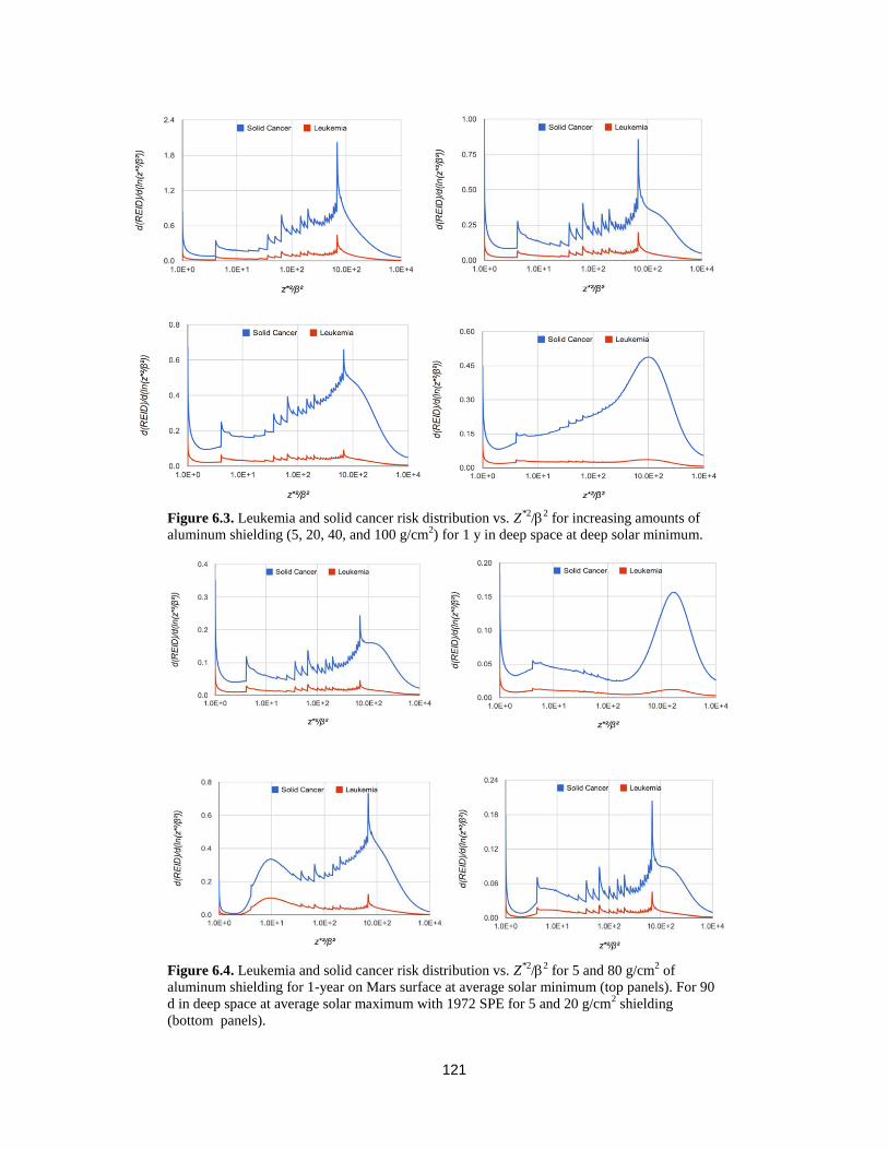
121

Figure 6.4. Leukemia and solid cancer risk distribution vs. Z*2

/2 for 5 and 80 g/cm

2 of

aluminum shielding for 1-year on Mars surface at average solar minimum (top panels). For 90

d in deep space at average solar maximum with 1972 SPE for 5 and 20 g/cm2 shielding

(bottom panels).

Figure 6.3. Leukemia and solid cancer risk distribution vs. Z

*2/

2 for increasing amounts of

aluminum shielding (5, 20, 40, and 100 g/cm2) for 1 y in deep space at deep solar minimum.

122

6.3 NASA Effective Dose and Tissue Weights

In the approach described above, tissue weights, wT, do not appear in the calculation of REID or REIC; however, because Effective dose is still a useful summary variable for mission operations, we estimated gender-specific wT values (Table 6.3) averaged over typical astronaut ages (30 to 60 y). The use of the terminology ―Effective dose‖ refers specifically to the ICRP definition. However, NASA continues to make adjustments to methods from the ICRP and NCRP based on the unique circumstances of space radiation protection. The use of this methodology with modified values is intended strictly for internal NASA usage and should be denoted ―NASA Effective Dose‖. Several differences in values for the tissue weights estimated here compared to the ICRP values. First, the ICRP includes hereditary risk and nonlethal cancer in its considerations of radiation detriment in recommending wT values. In comparison, NASA uses cancer-mortality-based risk limits (REID) based on NCRP recommendations.6 The ICRP averages tissue weights over age and gender, including values for pre-adults because its simplified methods are intended for use in both occupational and public exposures. Comparison of the ICRP values to gender-specific estimates in the NASA model for adults (30 to 60 y) are shown in Table 6.4. Distinct values would occur for different radiation fields because of the different QF used for the leukemia risk estimate. Never-smokers also have different tissue weights than the average U.S. population due to lower contributions from smoking-attributable cancers. The ICRP wT values for skin, gonad, and thyroid, which make negligible contributions to the REID, can lead to very high estimates of Effective doses for SPEs in which steep dose gradients occur, especially for extravehicular activity risk assessments. The values in Table 6.3 are good approximations for SPEs or trapped protons; however, for GCR, the leukemia weights are reduced and solid cancer weights are increased as indicated by values in parentheses. We compare calculations of annual Effective dose in the ICRP model to the NASA-recommended model for ISS missions at solar minimum and maximum in Figure 6.5. Comparisons for aluminum and polyethylene shielding are shown. The AP8 model of trapped protons is used, as is the Badhwar and O’Neill 2011 model of the GCR environment with quiet-time geomagnetic cutoffs. The CAM [computerized anatomical man] and CAF [computerized anatomical female] models of tissue self-shielding213 are used to evaluate of organ dose equivalents. The steep dose gradient at shallow depths for the ISS orbit is due to the trapped proton dose attenuation. Figure 6.6 shows similar comparisons for 1 y in deep space. The ICRP model, due largely to its higher estimation of contributions for relativistic particles than described here, provides higher estimates at shallow shielding depth. At deep shielding depths, the NASA model is larger due to its assignment of higher biological effectiveness to low-energy proton and helium nuclei produced by neutrons and other particles and from atomic slowing down of primaries. For the various mission scenarios, differences in Effective doses are on the order of 10% to 30%; however, the NASA model allows for a more precise uncertainty assessment to be made than the ICRP Q function, whose parameters are difficult to relate to biophysical interpretation. Figure 6.7 shows predictions of the Effective dose map on the surface of Mars using the MOLA [Mars orbiter laser altimeter] data to determine the vertical height of the carbon dioxide atmosphere and assuming a 10 g/cm2 aluminum habitat. Shown are results for the 1972 SPE using the King spectra (and the annual GCR at solar minimum). GCR Effective doses will be much larger than SPEs on the martian surface due to the attenuation of the SPEs by the martian atmosphere. Comparisons of Figure 6.7 will be useful for the selection of future crew landing sites on the Mars surface to minimize crew risks. Figure 6.8 compares the spectrum average QFs for the NASA and ICRP models for each charge group. The less attenuation at deep shielding depths in the NASA model is largely attributed to the increased biological effectiveness of low energy protons and helium particles produced in shielding and tissue.

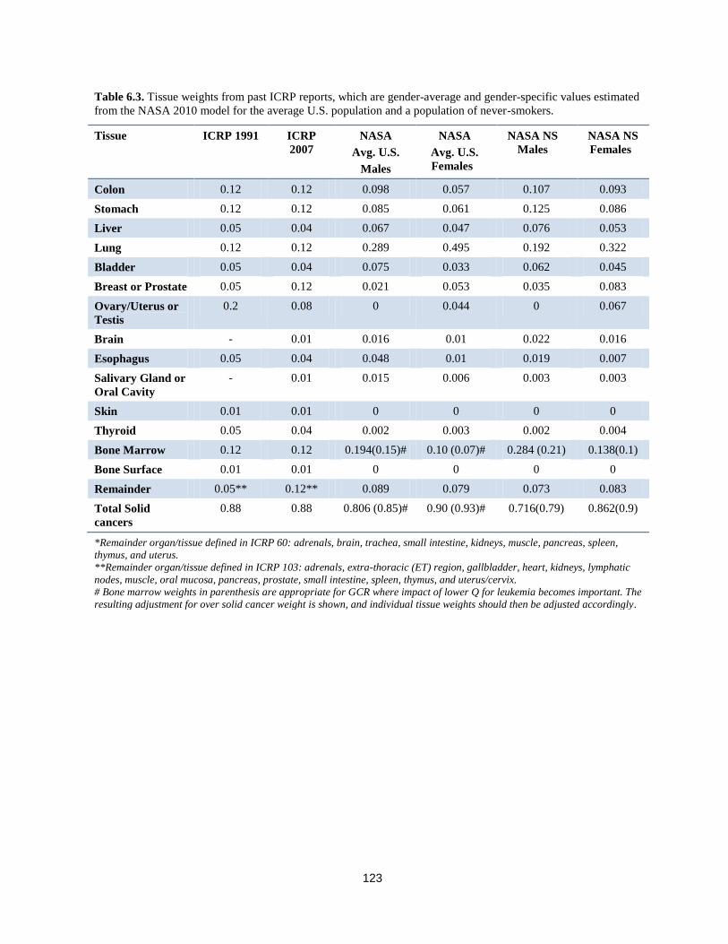
123

Table 6.3. Tissue weights from past ICRP reports, which are gender-average and gender-specific values estimated

from the NASA 2010 model for the average U.S. population and a population of never-smokers.

Tissue ICRP 1991 ICRP

2007

NASA

Avg. U.S.

Males

NASA

Avg. U.S.

Females

NASA NS

Males

NASA NS

Females

Colon 0.12 0.12 0.098 0.057 0.107 0.093

Stomach 0.12 0.12 0.085 0.061 0.125 0.086

Liver 0.05 0.04 0.067 0.047 0.076 0.053

Lung 0.12 0.12 0.289 0.495 0.192 0.322

Bladder 0.05 0.04 0.075 0.033 0.062 0.045

Breast or Prostate 0.05 0.12 0.021 0.053 0.035 0.083

Ovary/Uterus or

Testis

0.2 0.08 0 0.044 0 0.067

Brain - 0.01 0.016 0.01 0.022 0.016

Esophagus 0.05 0.04 0.048 0.01 0.019 0.007

Salivary Gland or

Oral Cavity

- 0.01 0.015 0.006 0.003 0.003

Skin 0.01 0.01 0 0 0 0

Thyroid 0.05 0.04 0.002 0.003 0.002 0.004

Bone Marrow 0.12 0.12 0.194(0.15)# 0.10 (0.07)# 0.284 (0.21) 0.138(0.1)

Bone Surface 0.01 0.01 0 0 0 0

Remainder 0.05** 0.12** 0.089 0.079 0.073 0.083

Total Solid

cancers

0.88 0.88 0.806 (0.85)# 0.90 (0.93)# 0.716(0.79) 0.862(0.9)

*Remainder organ/tissue defined in ICRP 60: adrenals, brain, trachea, small intestine, kidneys, muscle, pancreas, spleen,

thymus, and uterus.

**Remainder organ/tissue defined in ICRP 103: adrenals, extra-thoracic (ET) region, gallbladder, heart, kidneys, lymphatic

nodes, muscle, oral mucosa, pancreas, prostate, small intestine, spleen, thymus, and uterus/cervix.

# Bone marrow weights in parenthesis are appropriate for GCR where impact of lower Q for leukemia becomes important. The

resulting adjustment for over solid cancer weight is shown, and individual tissue weights should then be adjusted accordingly.

124

Figure 6.6. Annual GCR Effective doses or NASA Effective dose in deep space vs. depth of

shielding for males. Values for solar minimum and maximum are shown.

0

100

200

300

400

500

600

700

800

0 20 40 60 80 100

E, m

Sv/y

X, g/cm2

E(NASA)_AlE(ICRP)_AlE(NASA)_PEE(ICRP)_PEE(NASA)_AlE(ICRP)_AlE(NASA)_PESolar Minimum

Solar Maximum

Figure 6.5. Comparison of annual Effective dose or NASA Effective for males in ISS orbit (51.6 deg

400 km) vs. depth of shielding. Values for solar minimum and maximum are shown.

0

100

200

300

400

500

600

0 20 40 60 80 100

E, m

Sv/y

X, g/cm2

E(NASA)_Al

E(ICRP)_Al

E(NASA)_PE

E(ICRP)_PE

E(NASA)_Al

E(ICRP)_Al

E(NASA)_PE

E(ICRP)_PE

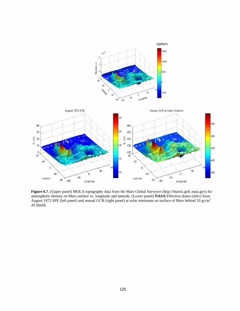
125

Figure 6.7. (Upper panel) MOLA topography data from the Mars Global Surveyor (http://tharsis.gsfc.nasa.gov) for

atmospheric density on Mars surface vs. longitude and latitude. (Lower panel) NASA Effective doses (mSv) from

August 1972 SPE (left panel) and annual GCR (right panel) at solar minimum on surface of Mars behind 10 g/cm2

Al shield.

meters

126

6.4 Overall Uncertainty Assessment

PDFs describing the uncertainties to the quantiles, x, for the various parameters in the model are described in Table 6.4. Space physics uncertainties were described in Chapter 2, low-LET uncertainties were described in Chapter 4, and radiation quality uncertainties were described in Chapter 5. The subjective PDFs are then employed in Monte-Carlo calculations to describe a given space radiation scenario, as described previously.12,14,15,20 Figures 5.18 and 5.19 illustrates the uncertainties in the Q value for solid cancer and leukemia, respectively vs. kinetic energy. The median values and 95% CIs are shown. The largest contributor to the Q-uncertainty is the

maximum value, Qmax, or the value of 0/. The point (central) estimates for Qmax of 40 or 10 for solid cancers or leukemia, respectively, occur for the most effective proton energy (~0.5 MeV). Values assigned give more weight to the animal model solid tumor data and are influenced by fractionation studies that suggest that higher RBEs are possible. These values are also consistent with RBEs for gene mutation and chromosomal aberrations in human cells. Possible contributions to uncertainties from NTE are discussed below. We did not consider uncertainty quantiles for the characteristic energy for thindown, Eth in Eq(5.19). Estimates of values for this parameter is likely

correlated with the values of m, ,and 0 /, and the addition of quantiles with small influence would not add to the analysis.214 The addition of a quantile for Eth would also create the complication of performing uncertainty analysis for each charge group, rather than the light and heavy charge groups considered here. The possible correlations between DDREF and Qmax (or

0/) are difficult to estimate with existing data; however, they should be considered in future work.

Figure 6.8. Spectra-tissue averaged central estimate of QF in the NASA model or ICRP QF for each charge group,

Z shown for 5 and 20 g/cm2 aluminum shielding. Calculations are made for the average solar minimum.

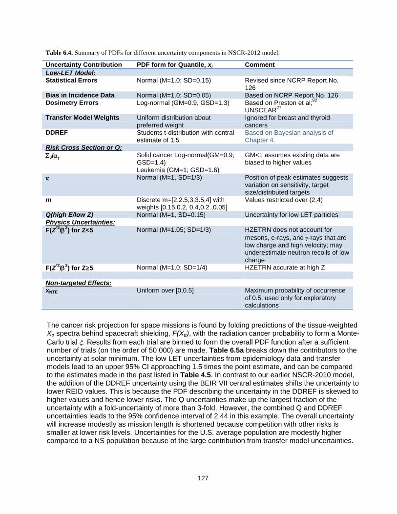
127

The cancer risk projection for space missions is found by folding predictions of the tissue-weighted Xtr spectra behind spacecraft shielding, F(Xtr), with the radiation cancer probability to form a Monte-

Carlo trial . Results from each trial are binned to form the overall PDF function after a sufficient number of trials (on the order of 50 000) are made. Table 6.5a breaks down the contributors to the uncertainty at solar minimum. The low-LET uncertainties from epidemiology data and transfer models lead to an upper 95% CI approaching 1.5 times the point estimate, and can be compared to the estimates made in the past listed in Table 4.5. In contrast to our earlier NSCR-2010 model, the addition of the DDREF uncertainty using the BEIR VII central estimates shifts the uncertainty to lower REID values. This is because the PDF describing the uncertainty in the DDREF is skewed to higher values and hence lower risks. The Q uncertainties make up the largest fraction of the uncertainty with a fold-uncertainty of more than 3-fold. However, the combined Q and DDREF uncertainties leads to the 95% confidence interval of 2.44 in this example. The overall uncertainty will increase modestly as mission length is shortened because competition with other risks is smaller at lower risk levels. Uncertainties for the U.S. average population are modestly higher compared to a NS population because of the large contribution from transfer model uncertainties.

Table 6.4. Summary of PDFs for different uncertainty components in NSCR-2012 model.

Uncertainty Contribution PDF form for Quantile, xj Comment

Low-LET Model: Statistical Errors Normal (M=1.0; SD=0.15) Revised since NCRP Report No.

126 Bias in Incidence Data Normal (M=1.0; SD=0.05) Based on NCRP Report No. 126 Dosimetry Errors Log-normal (GM=0.9, GSD=1.3) Based on Preston et al;

92

UNSCEAR27

Transfer Model Weights Uniform distribution about

preferred weight Ignored for breast and thyroid cancers

DDREF Students t-distribution with central estimate of 1.5

Based on Bayesian analysis of Chapter 4.

Risk Cross Section or Q:

0/ Solid cancer Log-normal(GM=0.9; GSD=1.4) Leukemia (GM=1; GSD=1.6)

GM<1 assumes existing data are biased to higher values

Normal (M=1, SD=1/3) Position of peak estimates suggests variation on sensitivity, target size/distributed targets

m Discrete m=[2,2.5,3,3.5,4] with weights [0.15,0.2, 0.4,0.2.,0.05]

Values restricted over (2,4)

Q(high E/low Z) Normal (M=1, SD=0.15) Uncertainty for low LET particles Physics Uncertainties:

F(Z*2

/2) for Z<5 Normal (M=1.05; SD=1/3) HZETRN does not account for

mesons, e-rays, and -rays that are low charge and high velocity; may underestimate neutron recoils of low charge

F(Z*2

/2) for Z5 Normal (M=1.0; SD=1/4) HZETRN accurate at high Z

Non-targeted Effects: xNTE Uniform over [0,0.5] Maximum probability of occurrence

of 0.5; used only for exploratory calculations

128

Table 6.5b shows comparisons near solar maximum, assuming the 1972 SPE occurred during a 1-y deep-space mission. Overall uncertainties are reduced compared to those of the GCR. In summary, these uncertainty estimates are reduced compared to the NSCR-2010 model, largely due to the smaller uncertainty in the Q-distribution and the skewness of the DDREF uncertainty to lower risk (higher DDREF). Table 6.6a shows estimates of the number of ―safe days‖ to be within the NASA limits at a 95% confidence level for NS and the average US population. Calculations are for 20 g/cm2 of aluminum shielding at the average solar minimum as described in Chapter 2 and in parenthesis for the recent 2009 deep solar minimum. The differences between the average and deep solar minima are small because the reduced solar modulation that occurs largely effects lower energy particles that are stopped by shielding or tissue. The gain in the number of safe days for never- smokers compared to the average U.S. population can be contrasted with the results of Figure 6.6 for large amounts of aluminum or polyethylene shielding. Results are improved compared to the NSCR-2010 model due to the improved BO11 model and changes that resulted from the NCR Report leading to the NSCR-2012 model as described above. Table 6.6b shows a similar comparison for the average solar maximum with or without exposure to the large 1972 SPE. The result without the SPE are reflective of a well-designed storm shelter that would eliminate most SPE exposure. Such storm shelter solutions have been known for many years and are practically implemented into spacecraft designs. Exploration missions near solar maximum are clearly favorable if sufficient SPE protection is provided, compared to missions near solar minimum. For both solar minimum and solar maximum conditions, gaining knowledge to improve risk assessments has the potential to lead to more substantial reductions in risk projections than the addition of costly radiation shielding or the use of alternative radiation shielding materials.

Table. 6.5b. Contributions of various uncertainties for 40-y females for the August 1972 SPE (King Spectra) in deep

space with a 10-g/cm2 aluminum shield.

Uncertainties considered

Expected Mean Median STD Lower 95%

Upper 95%

Fold Uncert.

Epidemiology, Transfer

1.12 0.87 0.81 0.32 0.27 1.56 1.39

Epidemiology, Transfer, DDREF

1.12 0.63 0.55 0.3 0.16 1.27 1.14

Q only 1.12 1.15 0.91 0.92 0.41 2.99 2.68 Q and Physics 1.12 1.17 0.91 0.95 0.45 3.10 2.77 All uncertainties 1.12 0.83 0.62 0.82 0.16 2.42 2.16

Table. 6.5a. Contributions of various uncertainties for 40-y females on a 1-y mission at solar minimum in deep space

with a 2-g/cm2 aluminum shield.

Uncertainties considered

Expected Mean Median STD Lower 95%

Upper 95%

Fold Uncert.

Epidemiology, Transfer

2.60 2.24 2.09 0.82 0.62 4.0 1.53

Epidemiology, Transfer, DDREF

2.60 1.59 1.36 0.76 0.40 3.37 1.30

Q only 2.60 2.85 2.24 2.22 0.92 7.96 3.06 Q and Physics 2.60 2.89 2.26 2.22 0.92 8.10 3.12 All uncertainties 2.60 2.03 1.50 1.92 0.40 6.34 2.44

129

Table 6.6b. Solar Maximum Safe Days in deep space, which are defined as the maximum

number of days with 95% CL to be below the NASA 3%REID limit. Calculations are for

average solar maximum assuming large August 1972 SPE with 20 g/cm2 aluminum

shielding. Values in parenthesis are the case without SPE that also represents the case of an

ideal storm shelter that reduce SPE doses to a negligible amount.

aE, y NASA 2012 U.S. Avg. Population


Males 35 306 (357) 395 (458) 45 344 (397) 456 (526) 55 367 (460) 500 (615)

Females 35 144 (187) 276 (325) 45 187 (232) 319 (394) 55 227 (282) 383 (472)

Table 6.6a. Solar Minimum Safe Days in deep space, which are defined as the maximum

number of days with 95% CL [confidence level] to be below the NASA 3%REID limit.

Calculations are for average solar minimum with 20 g/cm2 aluminum shielding. Values in

parenthesis are the case of the deep solar minimum of 2009.

aE, y NASA 2005 NASA 2012 U.S. Avg. Population


Males 35 158 209 (205) 271 (256) 45 207 232 (227) 308 (291) 55 302 274 (256) 351 (335)

Females 35 129 106 (95) 187 (180) 45 173 139 (125) 227 (212) 55 259 161 (159) 277 (246)

130

6.4.1 Uncertainties due to Non-targeted effects

To estimate the uncertainty contribution from NTEs, we introduced a dose-dependent QF trial function and an additional quantile representing the probability that NTEs contribute to cancer risks. Using the Harderian gland data as a basis for parameters for the uncertainty assessment, we assume, for a Monte-Carlo trial, the modified QF function:

(1 )NTE TE crossS S NTE

T

DQ Q x

D (6.8)

where the quantile, xNTE represents the uncertain contribution of NTEs to space radiation cancer risk. We assumed a uniform PDF for this quantile, but with a limited maximum probability of 0.5. We chose not to vary the parametric dependence of Dcross and used the Harderian gland estimates with no modifications. Figure 6.9 shows results for risks and uncertainties for absorbed doses of 0.01 and 0.1 Gy of 600 MeV/u Fe. Further comparisons are shown in Table 6.9. These results show that about a 2-fold increase in uncertainties compared to TEs alone occurs at low dose (<0.1 Gy) representative of GCR exposures. Extension of the calculations for mixed-particle space environment will depend not only on the NTE probability, but also on information on temporal aspects and likely lower dose or fluence (threshold) for NTE occurrence. Results could be higher or lower depending on these assumptions. The current recommendation is that research using chronic exposures to simulate GCR studying cancer-related processes should be prioritized because of the large impact of the results for NASA. Efforts to validate or refute the importance of NTEs should consider in-vivo experiments with representative tissues of human cancer risks, as well as differences between chronic and acute irradiation for small total absorbed doses (<0.3 Gy).

Figure 6.9. Uncertainty assessment for REID distribution for 600 MeV/u Fe nuclei at 0.01 or 0.1 Gy for 40-y males

with a limit of 0.5 for maximum probability that NTE occur and average probability of 0.25.

(%)REID per 0.1 Gy

0 10 20 30 40 50

(%)

Fre

quency

0.0

0.5

1.0

1.5

2.0

Epidem/DDREF Uncertainties

Epi/DDREF/QF-TE Uncertainties

With NTE Uncertainties

(%)REID per 0.01 Gy

0 2 4 6 8 10

(%)

Fre

quency

0.0

0.5

1.0

1.5

2.0

Epidem/DDREF Uncertainties

Epi/DDREF/QF-TE Uncertainties

With NTE Uncertainties

131

6.5 Considerations for Implementation of New Methods Implementation of the recommendations made in this report should consider several areas, including dosimetry requirements, application for the ISS Program, historical records or future epidemiology studies, and new or ongoing NASA trade studies for exploration mission planning. The NCRP recommends updating radiation worker records when revised assessments exceed potential changes of more than 30%.25 Our recommendations for Effective doses and REID pro-jections would include instances in which assessments would be above or below a 30% difference. Exposure records at NASA include mission dosimetry values, Effective dose and organ dose equivalents using the HZETRN/QMSFRG and CAM/CAF models,73 and projections of REID and REIC. It will be a small undertaking to reassess past ISS exposures and risk levels using the revised approach, but a much larger effort for past shuttle missions. Effective doses on shuttle missions were small – typically below 10 mSv. We recommend that exposures for the past and future ISS missions be updated using the new methods. For space shuttle and other past missions, there is no strong rationale to update organ dose equivalent records; however, REID and REID values could easily be updated using existing databases. For NASA trade studies, the approaches here are recommended for future mission analysis. Models of radiation risks and uncertainty analysis are subjective when applied to human risk estimates from space radiation. Nevertheless, it continues to be a reasonable approach to carry acceptable levels of risk as specific REID values, and to make uncertainty assessments of the upper 95% CL as an additional safety consideration. Trade studies can explore the value of potential mitigation measures to reduce uncertainty factors and REID projections, but radiobiological research remains the primary method to reduce uncertainties for all space missions. Dosimetry in space flight is complex because of the many types of particles and energies comprising space radiation. Mission dosimetry includes area and crew personnel dosimetry. Area dosimetry used in the past includes TEPCs, charged-particle hodoscopes to measure Z and E spectra over a limited range, and passive dosimeters made up of TLDs and CR-39 nuclear track detectors. Typically, passive dosimeters used as area detectors are also carried by crew members as their dosimeter of record. Each of these dosimeters can measure various aspects of the radiation environment in space, but none can measure all radiation components. Furthermore, cancer risks are evaluated at sensitive tissue sites, which, of course, are not directly measured and must be estimated with computer models. NASA thus uses area and crew dosimetry in conjunction with the HZETRN/QMSFRG code to make estimates of organ dose equivalents in which mission-

Table 6.9. Influence of NTE on average and upper 95% CL REID for 40-y males exposed to 0.01 Gy (1 rad) of

HZE nuclei for different average probability of NTE occurrence, PNTE.

PNTE %REID for 0.01 Gy of Fe (600 MeV/u) %REID for 0.01 Gy of Si (1000 MeV/u)

Avg. Upper 95% CL Avg. Upper 95% CL

0 1.02 4.41 0.50 2.29

0.1 1.19 5.39 0.56 2.48

0.2 1.58 7.27 0.67 2.74

0.25 1.81 7.84 0.73 2.86

0.35 2.34 8.44 0.89 3.02

0.5 3.31 8.83 1.19 3.18

132

specific predictions are normalized to the dosimetry of record.25 The recommendations of this report would not change this approach; however, the new NASA QFs and REID/ REIC calculations would be employed. Biodosimetry results from the ISS crew would be unchanged, and these results already include track structure effects described in this report. Implementation of the recommendation made in this report to estimate cancer risks and Effective dose limits for never-smokers should consider several factors. Ensuring continued never-smoker status for the remainder of a lifetime should be a minor concern because most individuals make a decision on tobacco usage at a young age. The influence of secondhand smoke and risks for former smokers also needs to be considered. The CDC has estimated the number of secondhand smoke-attributable cancers,101 which indicates that the number is a much smaller fraction of cancer risks than the corrections considered in this report. The potential impact of secondhand smoke should be emphasized in occupational health programs at NASA, however. The genetic basis for individual radiation sensitivity is an active research area, although there is no consensus on whether or how to use such information at this time. Other non-genetic factors besides tobacco usage that could modify cancer risks from space radiation are: the age of first pregnancy for breast cancer risks, and skin pigment and history of ultraviolet exposures for skin cancer risks. Possible interactions between these factors and space radiation exposures should be considered in future research.

133

7. Conclusions

Important changes to the calculation of cancer risks from space radiation were proposed in this report. Several of these changes are based on recent reports from international committees on low-LET radiation effects, or reanalysis of older heavy ion data sets with the notable exception of new data on leukemia and liver tumors induced by Fe nuclei.134 In addition, the recommendations of the 2012 NRC report216 reviewing the NASA model were considered. Several reviews2,3,5 summarize more recent radiobiology findings on the qualitative and quantitative differences between space radiation and terrestrial low-LET radiation. However, very few comprehensive data sets related to radiation quality or dose-rate modifiers from space radiation have been reported in recent years, although many new studies are in progress. Uncertainties, described as the ratio of the upper 95% CL to the point projection, were slightly improved from our earlier estimates, with improvements partially negated by higher assessments of LSS dosimetry errors in recent reports compared to the earlier NCRP assessment.15 GCR uncertainties estimates at solar minimum were about 2.4 to 2.6 fold in our revised assessment. The uncertainties in the DDREF and QF offset each other, with the DDREF uncertainty reducing the upper 95% CI, and the uncertainties in QF increasing the upper 95% CI in the NSCR-2012 model. The goal of the NASA Space Radiation Program (SRP) is to achieve less than a 50% error for risk projections for a Mars mission, which is estimated to be the necessary tolerance level because of the higher radiation risks associated with Mars exploration. The underlying scaling approach to the LSS and other human radio-epidemiology data used to estimate space radiation risks has an inherent uncertainty of approaching 2-fold, which is a severe limitation to the current approach to space radiation risk estimates. Thus, the current approach will need to be replaced in future to achieve the SRP goal for a Mars mission. Changes recommended, based on the available new information, include:

Revisions to low-LET risk coefficients to scale space radiation cancer risks, based largely on the UNSCEAR17 fits to the most recent LSS incidence data.

Use of incidence-based risk transfer from the LSS to an average U.S. population as recommended by the BEIR VII report.

Development of an alternative risk calculation for never-smokers that reduces radiation risks for lung, esophagus, oral cavity, and bladder cancers compared to calculations for the average U.S. population.

Revisions to PDFs for uncertainties from low-LET radiation, including a revised PDF for the solid-cancer-risk DDREF with a point estimate of DDREF=1.5, based on the BEIR VII report16 and NRC-2012 review,216 compared to the NCRP value of 2, A Bayesian analysis was performed in this report to describe the DDREF uncertainty.

Development of a track-structure-based model of radiation QFs and an alternative risk cross-section approach, which rely on both E and Z and not LET alone.

Recommendation of a lower QF for leukemia risk compared to solid cancer risks.

Revisions to uncertainty assessment for space physics and radiation QFs.

Use of probabilistic models of SPE size, frequency, and spectral parameters for mission design for a given set of mission parameters (solar cycle, mission length, and shielding).

The RERF in Hiroshima, Japan, made important updates to the LSS data within the last decade, including longer follow-up time and implementation of the DS02 dosimetry system.96 The BEIR VII, UNSCEAR, and RERF92 reported on models of incidence or mortality rates for these data sets.

134

The BEIR VII report16 ignored the age at exposure dependence in EAR and ERR functions above age 30 y, while arguing that the effects were small or the data lacked significant power to detect this effect. The UNSCEAR report27 used more general functions of age as well as age at exposure dependences of ERR and EAR functions to describe temporal effects, and also used a Bayesian model of dosimetry errors. UNSCEAR showed that its approach provided improved fits to the LSS incidence data in comparison to the mathematical functions used in the BEIR VII report. Because the UNSCEAR report did not consider several minor tissues that may be of interest for future attributable risk calculations for ISS crew and exploration planning, we used the RERF model92 for these tissues (esophagus, oral cavity, ovary, and uterus) and adjusted the remainder calculation accordingly. We used the BEIR VII recommended rates from meta-analysis of several populations, including the LSS data, for radiation risks of breast and thyroid cancer. The most significant change compared to the NCRP model6 is the use of incidence rates from the LSS to project mortality risks for astronauts. When using incidence-based transfer, cancer rates from the LSS are transferred to the current U.S. population and then converted to mortality risks using ratios of mortality-to-incidence in the U.S. for each tissue site. Mortality-based risk transfer was shown to lead to a much larger decrease in risk with increasing age at exposure compared to incidence-based risk transfer, while yielding similar results around ages 40 to 45 y. We prefer incidence-based risk transfer because these rates are more stable with time compared to mortality rates. Mortality rates have changed appreciably over time since 1945, and are likely to continue to change in future. Tissue-specific estimates also are needed for attributable risk calculations, which will be described in a future report. The role of early detection of cancers, including lung, colon and breast cancer, could lead to a significant reduction in REID estimates, however requires further understanding of the possible histological differences in HZE particle induced tumors compared to others. The EPA considered an alternative approach to converting incidence to mortality for breast cancer risk, which was considered in this report. The role of early detection of cancer, future changes in cure rates, and possible differences in histology of space radiation cancers with backgrounds cancers will be important considerations for the future. Tissue-specific incidence calculations offer improved representation of cancer risks from SPE exposures. In the past, Effective dose calculations were made by averaging organ dose equivalents using tissue weights, wT, recommended by the ICRP that are age and gender averaged. In the NSCR-2013 approach, Effective doses do not enter into risk calculations; instead, tissue-specific organ dose equivalents are used. For operational radiation protection purposes, Effective doses are useful summary variables, and NSCR-2012 describes of gender-specific tissue weights for an average population of ages 30 to 60 y representative of NASA crew ages, and alternative weights for never-smokers. The recommended wT values are important for SPE risk estimates, in which large dose gradients occur, often leading to high skin, thyroid, an gonad dose equivalents. Therefore, an overestimate of SPE fatal cancer risks occurs when calculated using the ICRP-defined Effective dose. In the recommended wT values, skin dose equivalent is absent and the values for the thyroid and gonad are reduced. Because astronauts and many other individuals should be considered as healthy workers, including never-smokers (lifetime use of tobacco below 100 cigarettes), we considered a possible variation in risks and dose limits that would occur due to the reference population used for estimates. After adjusting U.S. average cancer rates to remove smoking effects, radiation risks for lung, and other smoking-attributable cancers including esophagus, oral cavity, stomach, and bladder cancer, estimates were made using a mixture model. Competing risks were considered through adjustments for cancer, circulatory disease, and pulmonary diseases for NS, which modestly increases risks due to longer life span. Overall cancer risks were found to be more than 20% and 30% lower for males and females, respectively, for never-smokers compared to the average U.S.

135

population. NSCR-2012 calculates age- and gender-specific dose limits, based on incidence-based risk transfer for never-smokers. Other healthy work effects, including normal BMI, could modify these results by increasing risk probabilities at very advanced ages (>85 y); however, data on cancer rates at these ages carry large uncertainties. This analysis illustrates that gaining knowledge to improve risk transfer models, which entails knowledge of cancer initiation and promotion effects, could significantly reduce uncertainties in risk projections. Larger reductions than were estimated in this report could occur if higher weight is given to multiplicative risk transfer compared to the transfer weights used herein. The effects of secondhand smoke and post-mission use of tobacco need to be taken into account when considering distinct radiation limits based on never-smoker risk estimates. A large number of radiobiology experiments show that biological effects depend on both particle charge number and velocity (or kinetic energy) and not on LET alone. For many years, theoretically based track structure models have predicted this effect. In this report, we developed a simple approach to take into account track structure effects using the improved physical descriptor

of Z*2/2 and breaking risk calculations into distinct response models for light (Z )4 and heavy

(Z>4) charged nuclei. Finer groupings into individual charge spectra can be made in future as more data become available. The revised approach to QFs described here corrects an important shortcoming in the ICRP definition of QF. Deficiencies in the ICRP model included that: the LET value of the maximum Q was independent of Z, and the slope of the Q function with varying E is incorrect both on the ascending and the descending side of a peak value. The resulting NASA

model evaluates risks using particle spectra dependent on Z*2/2 for light and heavy nuclei groups, and the total absorbed dose at sensitive tissue sites. We recommended QFs for leukemia risks with much smaller values than for solid cancer risks, based on limited but important data from human, animal, and cellular studies. Although the revised calculations of NASA Effective doses differ by about 10% to 30% from the ICRP-recommended QFs for varying shielding thicknesses, these calculations lead to distinct conclusions on the effectiveness of radiation shielding, and improved methods to assess uncertainties and target critical experiments to further reduced uncertainties. As described in Chapter I, uncertainties in radiation cancer risk estimates can be classified into Type I to IV type uncertainties. For Type I uncertainties, there was an increased estimate of the LSS dosimetry errors in recent reports compared to the NCRP description in 1997.15 There are uncertainties related to estimating the fraction of the U.S. population that are current or former smokers, and the types of cancers attributable to tobacco usage and related relative risk factors. Models of these uncertainties should be the focus of future work. The area of individual sensitivity is not considered in current risk models, but is certainly an important goal of future research and radiation protection methods. Type III uncertainties include space physics, DDREF, and radiation quality uncertainties. Space physics uncertainties continue to be a minor component of the overall uncertainty. For very thick shielding, there is a need for continued analysis of particle production processes that produce largely low-LET radiation (eg, mesons, electrons, and photons) that are less well studied by space transport codes than are protons, neutrons, and heavy nuclei. QFs with values below unity may be appropriate at sufficiently high energy for electrons and photons, and should be considered in uncertainty assessments. DDREF values are based on subjective assessment of dose and dose-rate responses across available data sets (human epidemiology, animal studies, and cell culture studies). The ICRP117 and NCRP6 recommend DDREF values of 2. However, the recent BEIR VII report recommended a

136

DDREF of 1.5. The impact of a wide range of DDREF values can be evaluated through error assessment methods for uncertainty assessments. Based on the NRC recommendation,216 we used a central estimate from the BEIR VII report,16 and a PDF based on Bayesian analysis of select data described in this report. The ICRP QF is not informed by existing radiobiology data for HZE nuclei. Uncertainty analysis is improved in the revised approach as the underlying QF parameters are more readily related to results from radiobiology experiments than to an LET-based approach such as the ICRP model. An alternative uncertainty assessment was described that assumes that the energy where the maximum QF occurs for each Z is highly constrained. Existing experimental data for Fe nuclei were used to estimate the most likely value and its standard deviation, whereas the underlying track structure model was used to predict the position for other nuclei with lower Z. Our overall uncertainty assessment led to ratios of the upper 95% CL to central estimates varying from about 2.4 to 2.7 GCR behind 20-g/cm2 aluminum shielding dependent on gender and smoking status. Uncertainties for the DDREF and QF were toward lower or higher values of REID, respectively, thereby reducing the overall uncertainty. These results suggest research strategies to improve parameter uncertainties with well-defined particle choices can be made. Tissue-specific estimates of the

parameters 0 and using validated experimental models such as transgenic tumor models of human cancers and a human cell culture model of cancer processes would be optimal in estimating these parameters. Such data would narrow uncertainty factors substantially from current estimates. Alternative uncertainty assessment approaches such as Bayesian methods should be used in the design and analysis of such experiments. Our revised approach allows for REIC and REID estimates in terms of track-structure-dependent risk cross sections. Risk cross sections, which have been suggested by several biophysical models of heavy ion effects, are useful for considering the extrapolation of radiobiology data to low

doses. The changes recommended replacing LET with Z*2/2 for different charge groups, but do not lead to any inconsistencies with current space dosimetry approaches, which scale transport code prediction or organ exposure to crew dosimeters and area monitors. However, the recommended approach places more emphasis on measurements of Z and E spectra, which can be estimated using CR-39 plastic track detectors worn by crew, and area detectors such as particle hodoscopes that resolve charge and energy. These methods can also be used to validate the accuracy of radiation transport code predictions as has been described in the past.73 Uncertainties not addressed are the ―unknown‖ uncertainties discussed by the NCRP, and uncertainty factors related to the distinct time after exposure dependence of cancer risks with radiation quality. Very little information is available to understand how an earlier time of appearance of tumors would impact risk assessments. Uncertainties due to deviation from linearity at low doses of heavy ions were explored with calculations motivated by nontargeted effects. NTEs or qualitative differences between HZE particles and low LER radiation could increase uncertainties by more than 2-fold for HZE nuclei, and may also depend on mission length. NTEs are a potential ―game-changer‖ for NASA because they may impact radiation protection paradigms with regard to mission length and shielding. Research with chronic exposures at low doses in appropriate models is needed to better understand the importance of NTE in cancer risks. No recommendation to use NTEs for mission requirements is made at this time; however, NTEs should be considered when deciding on research emphasis.

Several other concerns arise to the current risk projections for a exploration missions. These additional concerns clearly substantiate the NASA approach to protect against the upper 95% confidence level in the cancer risk model. First, the uncertainty estimates made in this report did

137

not consider inter-dependencies of the various uncertainties (Type IV uncertainties). These are partially accounted for using the method of Monte-Carlo propagation of errors described in this report. However other possible inter-dependencies could occur, and therefore the current estimates could under-estimate the overall uncertainty. Furthermore the role of individual radiation sensitivity is not included in current risk estimates. Finally, the additional mortality and morbidity risks for non-cancer diseases such as central nervous system risks and circulatory diseases are major concerns because that could substantially increase REID values above the current central estimates.5,300 It is important to note that the risks to the central nervous system include both during mission risks and possible late effects that could confer significant morbidity and mortality on returning crew from deep space missions. These additional risks are highly uncertain at this time, and will require substantial research efforts including life span studies in animal models to determine their significance. Overall these additional concerns demonstrate that the NASA approach to protect against the upper 95% confidence level is by no means conservative and is prudent until these additional concerns are fully addressed.

138

8. References

1National Academy of Sciences Space Science Board, Report of the Task Group on the Biological Effects of

Space Radiation. Radiation Hazards to Crews on Interplanetary Mission. Washington DC: National Academy of Sciences; 1996.

2Cucinotta FA, Durante M. Cancer risk from exposure to galactic cosmic rays: implications for space

exploration by human beings. The Lancet Onc. 2006;7:431-435. 3Durante M, Cucinotta FA. Heavy ion carcinogenesis and human space exploration Nat Rev Cancer.

2008;8:465-472. 4Schimmerling W, Wilson JW, Cucinotta FA, Kim MH. Requirements for simulating space radiations

with particle accelerators. In: Fujitaka K, Majima H, Ando K, Yasuda H, Susuki M, eds. Risk Evaluation of Cosmic-ray Exposure in Long-Term Manned Space Mission. Tokyo: Kodansha Scientific Ltd.; 1999:1-16.

5Information Needed to Make Radiation Protection Recommendations for Space Missions Beyond Low-Earth

Orbit. Bethesda, Md: National Council on Radiation Protection and Measurements; 2006. NCRP Report No. 153.

6NCRP, Recommendations of Dose Limits for Low Earth Orbit. Bethesda, Md: National Council on Radiation

Protection and Measurements; 2000. NCRP Report No. 132.

7Cucinotta FA, Manuel F, Jones J, et al. Space radiation and cataracts in astronauts. Radiat Res. December

2001;156:460-466. 8Chylack LT, Peterson LE, Feiveson A, et al. NASCA Report 1: Cross-sectional study of relationship of

exposure to space radiation and risk of lens opacity. Radiat Res. 2009;172:10-20. 9Preston DL, Shimizu Y, Pierce DA, Suyumac A, Mabuchi K. Studies of mortality of Atomic bomb survivors.

Report 13: Solid cancer and noncancer disease mortality: 1950-1997. Radiat Res. 2003;160:381-407.

10

Little MP, Hoel DG, Molitor J, Boice JD, Wakeford R, Muirhead CR. New models for evaluation of radiation-induced lifetime cancer risk and its uncertainty employed in the UNSCEAR 2006 report. Radiat Res. 2008;169:660-676.

11

Yang VV, Ainsworth EJ. Late effects of heavy charged particles on the fine structure of the mouse coronary artery. Radiat Res. 1982;91:135-144.

12Cucinotta FA, Schimmerling W, Wilson JW, et al. Space radiation cancer risks and uncertainties for Mars

missions. Radiat Res. 2001;156:682-688. 13

Cucinotta FA, Schimmerling W, Wilson JW, Peterson LE, and Saganti PB. Uncertainties In estimates of the risks of late effects from space radiation. Adv Space Res. 2004,34:1383-1389.

14

Cucinotta FA, Kim MY, Ren L. Evaluating shielding effectiveness for reducing space radiation cancer risks. Radiat Meas. 2006;41:1173-1185.

15

NCRP. Uncertainties in Fatal Cancer Risk Estimates Used in Radiation Protection. Bethesda, Md: National Council on Radiation Protection and Measurements; 1997. NCRP Report No. 126.

http://www.ncbi.nlm.nih.gov/pubmed/18451812?ordinalpos=3&itool=EntrezSystem2.PEntrez.Pubmed.Pubmed_ResultsPanel.Pubmed_RVDocSum

139

16National Academy of Sciences Committee on the Biological Effects of Radiation. Health Risks From

Exposure to Low Levels of Ionizing Radiation (BEIR VII). Washington DC: National Academy of Sciences Press: 2006.

17

United Nations Scientific Committee on the Effects of Atomic Radiation. Sources and Effects of Ionizing Radiation. UNSCEAR 2006 Report to the General Assembly, with Scientific Annexes. New York, NY: United Nations; 2008.

18

Schimmerling W. Accepting space radiation risks. Radiat Env Biophys. 2010;49:325-329. 19

Vaeth M, Pierce DA. Calculating excess lifetime risk in relative risk models. Environ Health Per. 1990;87:83-94.

20

Peterson LE, Cucinotta FA. Monte Carlo mixture model of lifetime cancer incidence risks for radiation on shuttle and the International Space Station. Mutat Res. 1999;430:327-335.

21

NCRP. Potential Impact of Individual Genetic Susceptibility and Previous Radiation Exposure on Radiation Risk for Astronauts. Bethesda MD. National Council on Radiation Protection and Measurements; 2011. Report No. 167.

22

George KA, Elliott T, Kawata T, Pluth JM, Cucinotta FA. Biological effectiveness of low doses of -rays and iron nuclei for induction of chromosome aberrations in normal and repair deficient cell lines. Radiat. Res. 2009; 171:752-763.

23

Barcellos-Hoff MH, Park C, Wright EG. Radiation and the microenvironment – tumorigenesis and therapy. Nat Rev Cancer. 2005;5:867-875.

24

Cucinotta FA, Chappell LJ, Non-targeted effects and the dose response for heavy ion tumor formation. Mutat Res. 2010;687:49-53.

25

NCRP. Operational radiation protection in low Earth orbit. Bethesda, Md: National Council on Radiation Protection and Measurements; 2003. NCRP Report No. 142.

26

ICRP. 1990 Recommendations of the International Commission on Radiological Protection. Oxford: Pergamon Press; 1990. ICRP Publication 60.

27

Cucinotta FA, Hu S, Schwadron NA, Townsend LW, Kim MY. Space radiation risk limits and Earth-moon-Mars environmental models. Available at: http://www.agu.org/pubs/crossref/2010/2010SW000572.shtml. Accessed July 18, 2011.

28

Badhwar GD, Cucinotta FA. A comparison of depth dependence of dose and linear energy transfer spectra in aluminum and polyethylene. Radiat Res. 2000;153:1-8.

29

Wilson JW, Nealy JE, Atwell W, Cucinotta FA, Shinn JL, Townsend LW. Improved Model for solar Cosmic Ray Exposures in Manned Earth Orbital Flights. Houston, Tx: NASA Johnson Space Center; 1990. NASA TP-1990-2987.

30Cucinotta FA, Kim MH, Willingham V, George KA. Physical and biological organ dosimetry analysis for

International Space Station Astronauts. Radiat Res. 2008; 170: 127–138. 31

ICRP, Relative Biological Effectiveness (RBE), Quality Factor (Q), and Radiation Weighting Factor (wR). ICRP Publication 92. International Commission on Radiation Protection, Pergamon, 2003.

32

Rai SN, Kreqski D. Uncertainty and variability analysis in multiplicative risk models. Risk Analysis. 1998;18:37-45.

http://www.agu.org/pubs/crossref/2010/2010SW000572.shtml

http://www.ncbi.nlm.nih.gov/entrez/query.fcgi?cmd=Retrieve&db=pubmed&dopt=Abstract&list_uids=18582161

http://www.ncbi.nlm.nih.gov/entrez/query.fcgi?cmd=Retrieve&db=pubmed&dopt=Abstract&list_uids=18582161

140

33Wilson JW, Townsend LW, Schimmerling W, et al. Transport Methods and Interactions for Space

Radiations. Springfield, Va: National Technical Information Service, 1991. NASA RP-1257. 34

Cucinotta FA, Wilson JW, Williams JR, Dicello JF. Analysis of Mir-18 results for physical and biological dosimetry: radiation shielding effectiveness in LEO. Radiat Meas. 2000;132:181-191.

35

Ginzburg VL. The origin of cosmic radiation. Progr Elem Particle Cosmic Ray Phys. 1958;4:339. 36

Colgate SA, Grasberger WH, White RH. The dynamics of a supernova explosion. J Phys Soc Japan. 1963;17(suppl A-III):157.

37

Meyer P. Cosmic rays in the galaxy. Ann Rev Astron Astrophys. 1969;7:1. 38

Simpson JA. Elemental and isotropic composition of the galactic cosmic rays. In: Jackson J, Gove H, Schwitters R, eds. Ann Rev Nucl Particle Sci. 1983;33:323-381.

39

Cucinotta FA, Wilson JW, Saganti P, et al. Isotopic dependence of GCR fluence behind shielding. Radiat

Meas. 2006;41:1235-1249. 40

Webber WR, Southoul A, Ferrando P, Gupta M. The source charge and isotopic abundances of cosmic rays with Z = 9–16: a study using new fragmentation cross-sections. Astrophys J. 1990;348, 611-620.

41

Fields BD, Olive KA, Schramm DN. Cosmic ray models for early galactic lithium, beryllium and boron production. Astrophys J. 1994;435:185-202.

42

Wiedenback ME, Greiner DE. High-resolution observations of the isotopic composition of carbon and silicon in the galactic cosmic rays. Astrophys J. 1981;247:L119-L122.

43

Wiedenback ME. The isotopic composition on cosmic ray chlorine. Paper presented at: 19th International Cosmic Ray Conference; August 11-23, 1985; La Jolla, Calif.

44

Webber WR, Kish JC, Schrier DA. Cosmic ray isotope measurements with a new Cerenkov total energy telescope. Paper presented at: 19th International Cosmic Ray Conference; August 11-23, 1985; La Jolla, Calif.

45

Hesse A, Acarya BS, Heinbach U, et al. The isotopic composition of silicon and iron in the cosmic radiation as measured by the ALICE experiment. Proc 22nd Internat Cosmic Ray Conf (Dublin, Ireland). 1991;1:596-599 (1991).

46

Lukasiak A, Ferrando P, McDonald FB, Webber WR. Cosmic ray composition of 6<Z<8 nuclei in the energy range 50-150 MeV/n by the Voyager spacecraft during the solar minimum and maximum periods. Paper presented at: 23rd International Cosmic Ray Conference; July 19-30, 1993; La Jolla, Calif.

47

Lukasiak A, McDonald FB, Webber WR, Ferrando P. Voyager measurements of the isotopic composition of Sc, Ti, V, Cr, Mn, and Fe nuclei. Iucci N, Lamanna, eds. Proceedings of the Twenty-fourth International Cosmic Ray Conference. Vol. 2. Rome: International Union of Pure and Applied Physics; 1995:576-579.

48

Labrado AW, et al. Extended energy spectrum measurements of elements with the cosmic ray isotope spectrometer (CRIS). Proc 28th Int Cosmic Ray Conf (Tsukuba, Japan). 2003:1773-1776.

49

Zeitlin C, Cleghorn T, Cucinotta F, et al. Overview of the Martian radiation environment experiment. Adv Space Res. 2004;33:2204-2210.

141

50Badhwar GD, O’Neill PM. An improved model of GCR for space exploration missions. Nucl Tracks Radiat

Meas. 1992;20:403-410. 51

O’Neill P. Badhwar–O’Neill. Galactic cosmic ray model update based on advanced composition explorer (ACE) energy spectra from 1997 to present. Adv Space Res. 2006;37:1727-1733.

52Parker EN. The passage of energetic charged particles through interplanetary space. Planet Space Sci.

1965:13:9-49. 53

Bobcock HW. The topology of the Sun’s magnetic field and the 22-year cycle. Astrophys J. 1961;133(2):572-587.

54

Badhwar, G. B.; Cucinotta, F.A., and O'Neill, P. M.: An Analysis of Interplanetary Space Radiation Exposure for Various Solar Cycles. Radiat Res. 1994;138: 201-208.

55

Kim MY, De Angelis G, Cucinotta FA. Probabilistic risk assessment for astronauts on deep space missions. Acta Astron. 2011;68: 747-759.

56

Castagnoli GC, Cane D, Taricco C, Bhandari N. GCR flux decline during the last three centuries: extraterrestrial and terrestrial evidences. In: Kajita, T., Asaoka, Y., Kawachi, A., Matsubara, Y., Sasaki, M. (Eds.), GCR Flux Decline during the last Three Centuries: Extraterrestrial and Terrestrial Evidences. Universal Academy Press, Inc., 2003; 4045–4048.

57

Valtonen V, Nurmi P, Zheng JQ, et al. Natural transfer of viable microbes in space from planets in extra-solar systems to a planet in our solar system and vice versa. Astrophys J. 2009;690:210-215.

58

Forbush SE. On the effects in cosmic-ray intensity observed during the recent magnetic storm. Phys Rev. 1937;51:1108-1109.

59

Shea M, Smart DF. A summary of major proton events. Solar Phys. 1990;127:297-320. 60

Kim MY, Hayat MJ, Feiveson AH, Cucinotta FA. Prediction of frequency and exposure level of solar particle events. Health Phys. 2009;97:68-81.

61

McCracken KG, Dreschhoff G, Zeller EJ, Smart DF, Shea MA. 2001. Solar cosmic ray events for the period 1561-1994. 1. Identification in polar ice, 1561–1950. J Geophys Res. 2001;106(A10):21585-21598.

62

Goswami JN, McGuire RE, Reedy RC, Lal D, Jha R. Solar flare protons and alpha particles during the last three solar cycles. J Geophys Res. 1988;93:7195-7205.

63

National Geophysical Data Center (NGDC), National Oceanic and Atmospheric Administration (NOAA): GOES Space Environment Monitor (SEM) data archive directories. Available at: http://goes.ngdc.noaa.gov/data/. Accessed July 18, 2011.

64

Feynman J, Spitale G, Wang J, and S. Gabriel. Interplanetary proton fluence model: JPL 1991. J. Geophys Res. 1993, 98: 281-294.

65

King JH. Proton fluences for 1977-1983 space missions. J Spacecraft. 1974;11:401-408. 66

Wilson JW, Cucinotta FA, Kim M, Shinn JL, Jones TD, and Chang CK. Biological response to SPE exposure. Radiat Meas. 1999;30:361-370.

67

Band D, et al. Baste Observations of gamma-rays burst spectra. I. Spectral diversity. Astrophys J. 1993;413:281-292.

http://goes.ngdc.noaa.gov/data/

142

68Tylka AJ, Dietrich A. New comprehensive analysis of proton spectra in ground-level enhanced (GLE) solar

particle events. The Proceedings of the 31st International Cosmic Ray Conference, Lodz, Poland,

July 7-15, 1999. 69

Wilson JW, Kim MH, Schimmerling W, et al. Issues in space radiation protection. Health Phys. 1995;68:50-58.

70

Cucinotta FA, Plante I, Ponomarev AL, Kim MY. Nuclear interactions in heavy ion transport and event-based risk models. Radiat Prot Dosim. Doi: February 2011;143(2-4):384-390.

71Tripathi RK, Cucinotta FA, and Wilson JW. Accurate universal parameterization of absorption cross

sections. Nuclear Instrum Meth Phys Res. 1996; B117:347-349. 72

Cucinotta FA, Kim MY, Schneider SI, Hassler DM. Description of light ion production cross sections and fluxes on the Mars surface using the QMSFRG model. Radiat Environ Biophys. 2007;46:101-106.

73

Cucinotta FA, Wilson JW, Katz R, Atwell W, and Badhwar G D. Track structure and radiation transport models for space radiobiology studies. Adv Space Res. 1995;18:183-194.

74

Benton EV. Summary of radiation dosimetry results on the U.S. and Soviet manned spacecraft. Adv Space Res. 1986;6:315-328.

75

Zeitlin CJ, Sihver L, La Tessa C. Comparisons of fragmentation spectra using 1 GeV/amu 56

Fe data and the PHITS model. Radiat Meas. 2008;43:1242-1253.

76

Wilson JW, Cucinotta FA, Tai H, Shinn JL, Chun SY, Sihver L. Transport properties of light ions in matter. Adv Space Res. 1998;21:1763-1771.

77

Walker SA, Tweed J, Wilson JW. Validation of the HZETRN code for laboratory exposures with 1 GeV/u

iron with several targets. Adv Space Res. 2005;35:202-207. 78

Townsend LW, Miller TM, Gabriel TA. Modifications to the HETC radiation transport code for space radiation shielding applications: A status report. Paper presented at: 12th Biennial ANS Radiation Protection and Shielding Division Topical Meeting; April 14-18, 2002; Santa Fe, NM.

79

Ballarini F, Battistoni G, Brugger M, et al. The physics of the FLUKA code: recent developments. Adv Space Res. 2007;40:1339-1349.

80

Niita K, Sato T, Iwase H, Nose H, Nakashima H, Sihver L. PHITS – a particle and heavy ion transport code system. Radiat Meas. 2006;41:1080-1090.

81

Badhwar GD, Atwell W, Badavi FF, Yang TC, Cleghorn TF. Space radiation dose in a human phantom. Radiat Res. 2002;157:76-91.

82

Yasuda H, Badhwar GD, Komiyama T, Fujitaka K. Effective dose equivalent on the ninth shuttle-Mir mission (STS 91). Radiat Res. 2000;154:705-713.

83

Reitz G, et al. Astronaut's organ doses inferred from measurements in a human phantom outside the international space station. Radiat Res. 2009;171:225-235.

84

Badhwar GD, Patel JU, Cucinotta FA, Wilson JW. Measurements of secondary particle energy spectrum in the space shuttle. Radiat Meas. 1995;24:129-138.

85

Shinn JL, Badhwar GD, Xapsos MA, Cucinotta FA, Wilson JW. An analysis of energy deposition in a tissue equivalent proportional counter onboard the space shuttle. Radiat Meas. 1999;30:19-28.

http://www.ncbi.nlm.nih.gov/pubmed/19267549?ordinalpos=1&itool=EntrezSystem2.PEntrez.Pubmed.Pubmed_ResultsPanel.Pubmed_DefaultReportPanel.Pubmed_RVDocSum

http://www.ncbi.nlm.nih.gov/pubmed/19267549?ordinalpos=1&itool=EntrezSystem2.PEntrez.Pubmed.Pubmed_ResultsPanel.Pubmed_DefaultReportPanel.Pubmed_RVDocSum

143

86

Nikjoo H, Khvostunov IK, Cucinotta FA. The response of (TEPC) proportional counters to heavy ions. Radiat Res. 2002;157:435-445.

87

Wilson JW, et al. Time serial analysis of the induced LEO environment within the ISS 6A. Adv Space Res. 2007;40:1562-1570.

88

Kim MY, George KA, Cucinotta FA. Evaluation of skin cancer risks from lunar and Mars missions. Adv Space Res. 2006;37:1798-1803.

89Saganti PB, Cucinotta FA, Wilson JW, Simonsen LC, and Zeitlin CJ. Radiation climate map for analyzing

risks to astronauts on the Mars surface from galactic cosmic rays. Space Science Rev. 2004; 110:143-156.

90

Kim MY, Cucinotta FA, Wilson JW. A temporal forecast of radiation environments for future space exploration missions. Radiat Environ Biophys. 2007;46:95-100.

91

Ponomarev A, Nounu HN, Hussein HF, Kim MY, Atwell W, Cucinotta FA. NASA-developed ProE-based Tool for the Ray-tracing of Spacecraft Geometry to Determine Radiation Doses and Particle Fluxes in Habitable Area of Spacecraft and the Human Body. Houston, Tx: NASA Johnson Space Center; 2007. NASA TP-2007-214770.

92

Preston DL, Ron E, Tokuoka S, et al. Solid cancer incidence in atomic bomb survivors: 1958-1998. Radiat Res. 2007;168:1-64.

93

NIH. Report of the NCI-CDC Working Group to Revise the 1985 NIH Radioepidemiological Tables. Washington, DC: U.S. Department of Health and Human Services, National Institutes of Health, National Cancer Institute; 2003. NIH Publication No. 03-5387.

94

Little MP. Heterogeneity of variation of relative risk by age at exposure in the Japanese atomic bomb survivors. Radiat Environ Biophys. 2010;48:253-262.

95

Pawel D, Preston D, Pierce D, Cologne J. Improved estimates of cancer site-specific risks for A-bomb survivors. Radiat Res. 2008;169:87-98.

96

Preston DL, Pierce DA, Shimizu Y, et al. Recent changes in atomic bomb survivor dosimetry on cancer mortality risk estimates. Radiat Res. 2004;162:377–389.

97

Jacob P, Ruhm W, Walsh L, Blettner M, Hammer G, Zeeb H. Is cancer risk of radiation workers larger than expected? Occup Env Med. 2009;66:789-796.

98

NCRP. Guidance on Radiation Received in Space Activities. Bethesda, Md: National Council on Radiation Protection and Measurements; 1989. NCRP Report No. 98.

99

SEER, Surveillance, Epidemiology, and End Results: Cancer Statistics Review, 2005. Bethesda, Md: Cancer Surveillance Research Program, National Cancer Institute; 2006.

100

Kort EJ, Paneeth N, Vande Woude GF. The decline in U.S. cancer mortality in people born since 1925. Cancer Res. 2009;69:6500-6505.

101

Centers for Disease Control (CDC), Compressed Mortality File 1999-2005. CDC WONDER On-line Database, compiled from Compressed Mortality File 1999-2005 Series 20 No. 2K, 2008. Available at: http://wonder.cdc.gov/cmf-icd10.html. Accessed July 18, 2011.

102

Barcellos-Hoff MH, Ravini SA. Irradiated mammary gland stroma promotes the expression of tumorigenic potential by unirradiated epithelial cells. Cancer Res. 2000;60:1254-1260.

http://wonder.cdc.gov/cmf-icd10.html

144

103

Thun MJ, Hannan LM, Adams-Campbell LL, et al. Lung cancer occurrence in never-smokers: an analysis of 13 cohorts and 22 cancer registry studies. PLoS Med. 2008;5:1357-1371.

104

Furukawa K, Preston DL, Lonn S, et al. Radiation and smoking effects on lung cancer incidence among atomic bomb survivors. Radiat Res. 2010;174:72-82.

105

CDC-MMWR. Morbidity Weekly Report. Centers of Disease Control. 2008;57(45):1226-1228. 106

Terry PD, Rohan TE. Cigarette smoking and the risk of breast cancer in women: a review of the literature. Cancer Epidem Biomark Prev. 2002;11:953-971.

107

Subramanian J, Gavindan R. Molecular genetics of lung cancer in people who never have smoked. Lancet Oncol. 2008;9:676-682.

108

Land CE, Shimosatao Y, Saccomanno G, et. al. Radiation-associated lung cancer: a comparison of the histology of lung cancers in uranium miners and survivors of the atomic bombings of Hiroshima and Nagasaki. Radiat Res. 1993;134:234-243.

109

Gilbert ES, Stovall M, Gospodarowicz M, et al. Lung cancer after treatment for Hodgkin’s disease: focus on radiation effects. Radiat Res. 2003;159:161-173.

110

National Academy of Sciences, National Research Council, Committee on Health Risks of Exposure to Radon. Health Effects of Exposure to Radon (BEIR VI). Washington, DC: National Academy Press: 1999.

111

Preston DL, Krestnina LY, Sokolnikov ME, et al. How much can we say about site-specific cancer radiation risks? Radiat Res. 2010;174(6):816-824.

112

Suzuki, MS, Nomura T, Ejima Y, et al. Experimental derivation of relative biological effectiveness of A-bomb neutrons in Hiroshima and Nagasaki and Implications for risk assessment. Radiat Res. 2008;170: 101-117.

113

EPA. ‖EPA Radiogenic Cancer Risk Models and Projections for the U.S. Population‖. U.S. Environmental Protection Agency, Washington DC. (Draft report), 2008.

114

Kellerer AJ, Walsh L. Solid cancer risk coefficient for fast neutrons in terms of effective dose. Radiat Res 2002;158:61-68.

115

Goodhead DT, Thacker J, Cox R. Effectiveness of 0.3 keV carbon ultrasoft x-rays for the inactivation and mutation of cultured mammalian cells. Int J Radiat Biol. 1979;36:101–114.

116Hill MA. The variation in biological effectiveness of X-rays and gamma rays with energy. Radiat. Prot.

Dosim. 2004;112:471-481. 117

ICRP. The 2007 Recommendations of the International Commission on Radiological Protection. International Commission on Radiological Protection. Annals of the ICRP 37, Nos. 2-4; 2007. ICRP Publication 103.

118

Loucas BD, Eberle R, Bailey SM, Cornforth MN. Influence of dose rate on the induction of simple and complex chromosome exchanges by gamma rays. Radiat Res. 2004;162:339-349.

119

Cornforth M, Bailey SM, Goodwin EH. Dose responses for chromosome aberrations produced in noncycling primary human fibroblasts by alpha particles, and by gamma rays delivered at sublimiting low dose rates. Radiat Res. 2002; 158: 45-53.

145

120NCRP, Influence of Dose and Its Distribution in Time on Dose-Response Relationships for Low LET

Radiation. Bethesda, Md: National Council on Radiation Protection and Measurements; 1980. NCRP Report No. 64.

121

Storer JB, Mitchell TJ, Fry RJ. Extrapolation of the relative risk of radiogenic neoplasms across mouse strains and to man. Radiat Res. 1988;113:331-353.

122

Social Security Administration. A stochastic model of the long-range financial status of the OASDI program actuarial study no. 117. Washington, DC: Social Security Administration, Office of the Chief Actuary; September 2004. SSA Pub. No. 11-11555.

123

Yamane GK. Cancer incidence in the U.S. Air Force: 1989-2002. Aviat Space Env Med. 2006;77:789-794. 124

Bissell M, et al. Modeling Human Risk: Cell & Molecular Biology in Context. NASA and LBNL Publication 40278; Oak Ridge, TN. 1997.

125

Fry RJM, Storer JB. External radiation carcinogenesis. In: Lett JT, ed. Advances in Radiation Biology. Vol. 13. New York, NY: Academic Press; 1987:31-90.

126

Boice JD Jr. Leukemia risks in thorotrast patients. Radiat Res. 1993;136:301-302. 127

Grogan HA, Sinclair WK, Voilleque PG. Risks of fatal cancer from inhalation of 239,240

plutonium by humans: a combined four-method approach with uncertainty evaluation. Health Phys. 2001;80:447-461.

128

Burns F, Yin Y, Garte SJ, Hosselet S. Estimation of risk based on multiple events in radiation carcinogenesis of rat skin. Adv Space Res. 1994;14:507–519.

129

Burns FJ, Jin Y, Koenig KL et al. The low carcinogenicity of electron radiation relative to argon ions in rat skin. Radiat Res. 1993;135:178-188.

130Fry RJM, Powers-Risius P, Alpen EL, Ainsworth EJ. High LET radiation carcinogenesis. Radiat Res.

1985;104:S188-S195. 131

Alpen EL, Powers-Risius P, Curtis SB, DeGuzman R. Tumorigenic potential of high-Z, high-LET charged particle radiations. Radiat Res. 1993;88:132-143.

132

Alpen EL, Powers-Risius P, Curtis SB, DeGuzman R, Fry RJM. Fluence-based relative biological effectiveness for charged particle carcinogenesis in mouse Harderian gland. Adv Space Res. 1994;14:573-581.

133

Dicello JF, et al. In vivo mammary tumorigenesis in the Sprague-Dawley rat and microdosimetric correlates. Phys Med Biol. 2004;49:3817-3830.

134

Weil MM, Bedford JS, Bielefeldt-Ohmann H, Ray AF, Gernik PC, Ehrhart EJ, Falgren CM, Hailu F, Battaglia CLR, Charles C, Callan MA, Ullrich RLet al. Incidence of acute myeloid leukemia and hepatocellular carcinoma in mice irradiated with 1 GeV/nucleon

56Fe ions. Radiat Res.

2009;172:213-219. 135

Ainsworth EJ. Early and late mammalian responses to heavy charged particles. Adv Space Res. 1986;6:153-162.

136

Burns FJ, Hosselet S, Jin Y, Dudas G, Garte SJ. Progression and multiple events in radiation carcinogenesis of rat skin. J Radiat Res. 1991;32:S202–S216.

146

137Burns F, Zhao P, Xu G, Roy N, Loomis C. Fibroma induction in rat skin following single or multiple doses

of 1.0 GeV/nucleon 56

Fe ions from the Brookhaven alternating gradient synchrotron. Physica Medica. 2001;XVII:194-195.

138

Mole RH, Papworth, DG Corp MJ. The dose-response for X-ray induction of myeloid-leukemia in male CBA/H mice. Br. J. Cancer 1983;47:285–291.

139

Ullrich RL Preston RJ. Myeloid leukemia in male RFM mice following irradiation with fission spectrum neutrons or gamma rays. Radiat Res. 1987;109:165–170.

140

Griffiths SD, Marsden SJ, Wright EG, Greaves MF, Goodhead DT. Lethality and mutagenesis of B

lymphocyte progenitor cells following exposures to -particles and X-rays. Int J Radiat Biol. 1994;66:197-205.

141

Peng, Y, Brown N, Finnon, F et al., Radiation leukemogenesis in mice: Loss of PU.1 on chromosome 2 in

CBA and C57BL/6 mice after irradiation with 1 GeV/nucleon 56Fe ions, X rays or rays. Part I. experimental observations. Radiat Res. 2009; 171:474–483.

142

Edwards AA. RBE of space radiations and the implications for space travel. Physica Medica. 2001;XVII(suppl 1):147-152.

143

Fry RJM, Garcia AG, Allen KH, et al. The effect of pituitary isografts on radiation carcinogenesis in the mammary and Harderian glands of mice. In: Biological Effects of Low Level Radiation Pertinent to Protection of Man and His Environment. Vol. I. Vienna, Austria: International Atomic Energy Agency; 1976:213-227.

144

George KA, Cucinotta FA. The influence of shielding on the biological effectiveness of accelerated particles for the induction of chromosome damage. Adv Space Res. 2007;39:1076-1081.

145

George K, Durante M, Willingham V, Wu H, Yang T, Cucinotta FA. Biological effectiveness of accelerated particles for the induction of chromosome damage measured in metaphase and interphase human lymphocytes. Radiat Res. 2003;160:425-435.

146

Yang TC, Craise LM, Mei M, Tobias CA. Neoplastic cell transformation by heavy charged particles. Radiat Res. 1985;104:S177-S187.

147

Kiefer J, Stoll U, Schneider E. Mutation induction by heavy Ions. Adv Space Res. 1994;14(10):257-265. 148

Kiefer J, Schmidt P, Koch S. Mutations in mammalian cells induced by heavy charged particles: An indicator for risk Assessment in Space. Radiat Res. 2001;156:607-611.

149

Cucinotta FA, Wilson JW, Shavers MR, Katz R. Effects of track structure and cell inactivation on the calculation of heavy ion mutation rates in mammalian cells. Int J Radiat Biol. 1996;69:593-600.

150

Anderson R, Stevens DL, Goodhead DT. M-FISH analysis shows that complex chromosome aberrations induced by α-particle tracks are cumulative products of localized rearrangements. Proc Natl Acad Sci USA. 2002;99:12167-12172.

151

Durante M, George K, Wu H, Cucinotta FA. Karyotypes of human lymphocytes exposed to high-energy iron ions. Radiat Res. 2002;158:581-590.

152

Durante M, George K, and Cucinotta FA. Chromosomes lacking telomeres are present in the progeny of human lymphocytes exposed to heavy ions. Radiat Res. 2006;165:51-58.

153

Kadhim MA, Macdonald DA, Goodhead DT, Lorimore SA, Marsden SJ, Wright EG. Transmission of chromosomal instability after plutonium a-particle irradiation. Nature. 1992;355:738-740.

147

154

Watson GE, Lorimore SA, Clutton S, Kadhim M, Wright EG. Chromosomal instability in unirradiated cells induced in vivo by a bystander effect of ionizing radiation. Cancer Res. 2000;60:5608-5611.

155

Ullrich RL, Ponnaiya B. Radiation-induced instability and its relation to radiation carcinogenesis. Inter J Radiat Biol. 1998;74:747-754.

156

Brooks AL, Bao S, Rithidech K, Couch LA, Braby LA. Relative effectiveness of HZE iron-56 particles for the induction of cytogenetic damage in vivo. Radiat Res. 2001;155:353-359.

157

Evans HH, Horng M, Ricanati M, Diaz-Insua R, Scwarz JL. Characteristics of genomic instability in clones of TK6 human lymphoblasts surviving exposure to

56Fe ions. Radiat Res. 2002;158:687-698.

158

Sudo H, Garbe J, Stampfer MR, Barcellos-Hoff MH, Kronenberg A. Karyotypic instability and centrosome aberrations in the progeny of finite life-span human mammary epithelial cells exposed to sparsely or densely ionizing radiation. Radiat Res. 2008;170:23-32.

159

Ullrich RL. Tumor induction in BAL/c mice after fractionated neutron or gamma irradiation. Radiat Res. 1984;93:506-512.

160

NCRP. Relative Biological Effectiveness of Radiations of Different Quality. Bethesda, Md: National Council on Radiation Protection and Measurements; 1990. NCRP Report No. 104.

161

Cucinotta FA, Wilson JW. Initiation-promotion model for tumor prevalence from high energy and charge radiation. Phys Med Biol. 1994;39:1811-1831.

162

Katz R, Ackerson B, Homayoonfar M, Scharma SC. Inactivation of cells by heavy ion bombardment. Radiat Res. 1971;47:402-425.

163

Goodhead DT, Nikjoo H. Track structure analysis of ultrasoft X-rays compared to high- and low-LET radiations. Int J Radiat Biol. 1989;55:513-529.

164

Plante I, Cucinotta FA. Ionization and excitation cross sections for the interaction of HZE particles in liquid water and application to Monte-Carlo simulation of radiation tracks. New J Phys. 2008;10:125020 doi: 10.1088/1367-2630/10/12/125020.

165

Butts JJ, Katz R. Theory of RBE for heavy ion bombardment of dry enzymes and viruses. Radiat Res. 1967;30:855-871.

166

Cheung WK, Norbury JW. Stopping powers and cross sections due to two-photon processes in relativistic nucleus-nucleus collisions. Washington DC: NASA Headquarters, 1994. NASA CP 4574.

167

Kobetich R, Katz R. Energy deposition by electron beams and -rays. Phys Rev. 1968;170:391-396. 168

Brandt W, Ritchie HR. Primary processes in the physical stage. In: Cooper RD, Woods R, eds. Physical Mechanisms in Radiation Biology. Washington, DC: Technical Information Center, Atomic Energy Commission, U.S. Department of Energy; 1974:20-29.

169

Cucinotta FA, Nikjoo H, Goodhead DT. Applications of amorphous track models in radiobiology. Radiat Environ Biophys. 1999;38:81-92.

170

Chatterjee A, Maccabee D, Tobias CA. Radial cutoff LET and radial cutoff dose calculations for heavy charged particles in water. Radiat Res. 1973;54:479-494.

171

Kraft G, Kramer M. LET and track structure. In: Lett J, Sinclair WK, eds. Advances in Radiation Biology. San Diego, Calif: Academic Press; 1993:1-50.

http://dx.doi.org/10.1088/1367-2630/10/12/125020

148

172

Cucinotta FA, Nikjoo H, Goodhead DT. Model of the radial distribution of energy imparted in nanometer volumes from HZE particles. Radiat Res. 2000;153:459-468.

173

Goodhead DT, Munson RJ, Thacker J, Cox R. Mutation and inactivation of cultured mammalian cells exposed to beams of accelerated heavy ions. IV. Biophysical interpretation. Int J Radiat Biol. 1980;37:135-167.

174Katz R RBE, LET, and z/. Health Phys. 1970;18:175.

175

Thacker J, Stretch A, Stephens MA. Mutation and inactivation of cultured mammalian cells exposed to beams of accelerated heavy ions. II. Chinese hamster V79 cells. Int J Radiat Biol. 1979;38:137-148.

176

Belli M, Goodhead DT, Ianzini F, Simone G, Tabocchini MA. Direct comparison of biological effectiveness of protons and alpha-particles of the same LET. II. Mutation induction at the HPRT locus in V79 cells. Int J Radiat Biol. 1992;61:625-629.

177

Belli M, Cera F, Cherubini R, et al. Inactivation and mutation induction In V79 cells by low energy protons: re-evaluation of the results at the LNL facility. Int J Radiat Biol. 1993;63:331-337.

178

Schafer M, Schmitz C, Bucker H. DNA double strand breaks induced in Escherichia Coli cells by radiations of different quality. Radiat Prot Dosim. 1994;52:233-236.

179

Baltschukat K, Horneck G. Response to accelerated heavy ions of spores of Bacillus-Subtilis of different repair capacity. Radiat Env Biophys. 1991;30:87-104.

180

Kranert T, Schneider E, Kiefer J. Mutation induction in V79 Chinese hamster cells by very heavy ions. Int J Radiat Biol. 1990;58:975-987.

181

Cucinotta FA, Wilson JW, Shavers MR, Katz R. The Calculation of Heavy Ion Inactivation and Mutation Rates in the Track Structure Model. Houston, Tex: NASA Johnson Space Center; 1997. NASA TP-1997-3630.

182

Holley WR, Chatterjee A. Clusters of DNA damage induced by ionizing radiation: formation of short DNA fragments. I. Theoretical modeling. Radiat Res. 1996;145:188-189.

183

LaVerne JA. Review: Track effects of heavy ions in liquid water. Radiat Res. 2000;153:487-496. 184

Katz R, Cucinotta FA. RBE vs. dose for low doses of high LET radiation. Health Phys. 1991;60:717-719. 185

Katz R, Zachariah R, Cucinotta FA, Chanxiang Z. Survey of radiosensitivity parameters. Radiat Res. 1994;14:356-365.

186

Goodhead DT. Relationship of radiation track structure to biological effect: a re-interpretation of the parameters of the Katz model. Nuclear Tracks Radiat Meas. 1989;116:177-184.

187

Goodhead DT. Energy deposition stochastics and track structure: What about the target? Radiat Prot Dosim. 2006;122:3-15.

188

Wilson JW, Cucinotta FA, Shinn JL. Cell kinetics and track structure. In: Swenberg CE, et al, eds. Biological Effects and Physics of Solar and Galactic Cosmic Rays. New York, NY: Plenum Press, New York; 1993:295-338.

189

Cucinotta FA, Wilson JW. Initiation-promotion model of tumor prevalence in mice from space radiation exposure. Radiat Environ Biophys. 1995;34:145-149.

149

190Morgan WF. Non-targeted and delayed effects of exposure to ionizing radiation: I. Radiation-induced

genomic instability and bystander effects in vitro. Radiat Res.2003;159:567-580. 191

Prise KM, Belyakov OV, Folkard M, Michael BD. Studies on bystander effects in human fibroblasts using a charged particle microbeam. Int J Radiat Biol. 1998;74:793-798.

192

Belyakov OV, et al. Biological effects of unirradiated human tissue by radiation damage up to 1 mm away. Proc Natl Acad Sci USA. 2005;102:14203-14208.

193

Nagasawa H, Little JB. Induction of sister chromatid exchanges by extremely low doses of α-particles. Cancer Res. 1992;52:6394-6396.

194

Lehnert BE, Goodwin EH, Desphande A. Extracellular factors following exposure to α-particles can cause sister chromatid exchanges in normal human cells. Cancer Res. 1997;57:2164-2171.

195

Nagasawa H, Little JB. Bystander effect for chromosomal aberrations induced in wild-type and repair deficient CHO cells by low fluences of alpha particles. Mutat Res. 2002;508:121-129.

196

Miller RC, Marino SA, Brenner DJ, et al. The biological effectiveness of radon-progeny alpha particles. II. Oncogenic transformation as a function of linear energy transfer. Radiat Res. 1995;142:54-60.

197

Brenner DJ, Little JB, Sachs RK. The bystander effect in radiation oncogenesis. II. A quantitative model. Radiat Res. 2001;155:402-408.

198

Katz R, Scharma SC, Homayoonfar M. The structure of particle tracks. In: Attix FH, ed. Topics in Radiation Dosimetry, Supplement 1. New York, NY: Academic Press; 1972:317-383.

199

Hoffman W, Katz R, Chunxiang Z. Lung cancer risk at low doses of -particles. Health Phys. 1986;51:457-468.

200

Curtis SB, Nealy JE, Wilson JW. Risk cross sections and their application to risk estimation in the galactic cosmic-ray environment. Radiat Res. 1995;141:57-65.

201

NCRP. Fluence-based Microdosimetric Event-based Methods for Radiation Protection in Space. Bethesda, Md: National Council on Radiation Protection and Measurements; 2001. NCRP Report No. 137.

202

Edwards AA. The use of chromosomal aberrations in human lymphocytes for biological dosimetry. Radiat Res. 1997;148:S39-S44.

203

Sasaki MS, Takatsuji T, Ejima Y. The F value cannot be ruled out as a chromosomal fingerprint of radiation quality. Radiat Res. 1998;150:253-258.

204

Cox R, Masson WK. Mutation and inactivation of cultured mammalian cells exposed to beams of accelerated heavy Ions. Int J Radiat Biol. 1979;36:149-160.

205

Tsuboi K., Yang TC, Chen DJ. Charged-particle mutagenesis. I. cytoxic and mutagenic effects of high-LET charged iron particles on human skin fibroblasts. Radiat Res. 1992;129:171-176.

206

Kronenberg A. Mutation induction in human lymphoid cells by energetic heavy ions. Adv Space Res. 1994;14:339-346.

207

Yang TC, Craise LM, Mei M, Tobias CA. Neoplastic transformation by high LET radiation: Molecular mechanisms. Adv Space Res. 1989;9:131-140.

150

208Miller RC, Marino S., Brenner DJ, et al. The biological effectiveness of radon-progeny alpha particles III.

quality factors. Radiat. Res.1995;142: 61–69. 209

Waligorski MP, Sinclair GL, Katz R. Radiosensitivity parameters for neoplastic transformations in C3H10T1/2 cells. Radiat Res. 1987;111:424-437.

210

Barkas H. Nuclear Research Emulsions. Vol. 1. New York, NY: Academic Press Inc.; 1963:chap 9. 211

SEER, Horner MJ, Ries LAG, Krapcho M, Neyman N, Aminou R, Howlader N, Altekruse SF, Feuer EJ, Huang L, Mariotto A, Miller BA, Lewis DR, Eisner MP, Stinchcomb DG, Edwards BK (eds). SEER Cancer Statistics Review, 1975-2006, National Cancer Institute. Bethesda, MD, http://seer.cancer.gov/csr/1975_2006/, based on November 2008 SEER data submission, posted to the SEER web site, 2009

212

Han, Z, Suzuki H, Suzuki F, et al. Neoplastic transformation of hamster embryo cells by heavy ions. Adv Space Res. 1998;22:1725-1732.

213

Billings MP, Yucker WR, Heckman BR. Body self-shielding data analysis. Huntington Beach, Calif: McDonald Douglas Astronautics Company West; 1973. MDC-G4131.

214

Smith AE, Ryan PB, Evans JS. The effect of neglecting correlations when propagating uncertainty and estimating the population distribution of risk. Risk Analysis. 1992;12:467-474.

Added References: 215

Cucinotta FA, Kim MY, and Chappell LJ. Space radiation cancer risks and uncertainties- 2010. National Aeronautics and Space Administration, Washington DC. NASA TP-2011-216155.

216

National Research Council, Technical Evaluation of the NASA Model for Cancer Risk to Astronauts Due to Space Radiation. The National Academies Press, Washington D.C., 2012.

217

Hassler DM, Zeitlin CJ, Wimmer-Schweingruber K, Bottcher S, Martin C, Andres J, Bohm E, Brinza DE, Bullock MA, Burmeister S, Ehresmann B, Epperly M, Grinspoon D, Kohler G, Neal K, Peterson J, Posner A, Ratkin S, Seimetz L, Smith KD, Tyler Y, Weighle G, Reitz G, Cucinotta FA. The Radiation Assessment Detector (RAD) investigation. Space Science Rev. 2012; DOI: 10.1007/s11214-012-9913-1.

218

Schwadron NA, Townsend LW, Kozarev K, Dayeh MA, Cucinotta FA, Desai R, Golightly MJ, Hassler D, Hatcher R, Kim MY, Posner A, PourArsalan M, Spence HE, Squier RK. The Earth Moon Mars radiation environment module framework. Space Weather J. 2010; 8: S00E02, doi:10.1029/2009SW00052.

219

Kim MY, Hayat

ML, Feiveson AH, and Cucinotta FA. Using high-energy proton fluence to improve risk

prediction for consequences of solar particle events. Adv Space Res. 2009; 44: 1428-1432. 220

EPA, The Environmental Protection Agency’s (EPA’s) Report EPA Radiogenic Cancer Risk Models and Projections for the U.S. Population, 2011.

221

Cucinotta FA, and Chappell LJ. Updates to radiation risks limits for astronauts: risks for never-smokers. Radiat Res. 2011; 176:102‐114.

222

Cucinotta FA, Chappell LJ, Kim MY, and Wang M. Radiation carcinogenesis risk assessments for never-smokers. Health Phys. 2012; 103: 643-651.

223

IARC, International Agency for Research on Cancer. Tobacco smoking. IARC Monographs on the Evaluation of Carcinogenic Risks to Humans. Vol. 38. Lyon (France): IARC; 1986.

151

224

Pierce DA, Sharp GB, Mabuchi K. Joint effects of radiation and smoking on lung cancer risk among atomic bomb survivors. Radiat Res. 2003;159:511-520.

225

O’Neill PM. Badhwar-O’Neill 2010 galactic cosmic ray flux model- Revised. IEEE Trans Nucl Sci. 2010; 57.

226

George JS, Lave KA, Wiedenbeck ME, Binns WR, Cummings AC, et al. Elemental composition and energy spectra of galactic cosmic rays during solar cycle 23. Astrophys J. 2009; 696:1666-1681.

227

Nymmik RA, Panasyuk MI, Suslov AA. Galactic cosmic ray flux simulation and prediction. Adv Space Res. 1996; 30:219-230.

228

Adriani O, Barbarino GC, Bazilevskaya GA, Bellotti R, Boezio M, et al., PAMELA measurements of cosmic-ray proton and helium spectra. Science 2011; 332:69-72.

229

Menn W, Hof M, Reimer O, Simon M, Davis AJ, et al., The absolute flux of protons and helium at the top of the atmosphere using IMAX. Astrophys J. 2000; 533:281-297.

230

Boeizio M, Carlson P, Francke T, Weber N, Stuffert M, et al. The cosmic-ray proton and helium spectra between 0.4 and 200 GV. Astrophys J. 1999; 518:457-472.

231

Sanuki T., Motoki M, Matsumoto H, Seo ES, Wang JZ, et al. Precise measurement of cosmic-ray proton and helium spectra with the BESS spectrometer. Astrophys J. 2000; 545:1135-1142.

232

Aghara SK, Blattnig SR, Norbury JW, Singleterry RC. Monte Carlo Analysis of Pion Contribution to Absorbed Dose from Galactic Cosmic Rays. Nucl Instrum Meth Phys Res Sec B. 2009; 264:1115-1124.

233

Slaba T, Blattnig S, Reddell B, Bahadori A, Norman R, Badavi F. Pion and electromagnetic contribution to dose: comparisons of HZETRN to Monte Carlo results and ISS data. NASA TP (in press), 2012.

234

Sato T, Endo A, Sihver L, Niita K. Dose estimation for astronauts using dose conversion coefficients calculated with the PHITS code and the ICRP/ICRU adult reference computational phantoms. Radiat Environ Biophys. 2011; 50:115-123

235

Bryant A, Cerfolio RJ. Differences in epidemiology, histology, and survival between cigarette smokers and never-smokers who develop non-small cell lung cancer. Chest. 2007; 132:185-192.

236

2007 US Cancer and Mortality Statistics: 1999-2008 CDC WONDER Online Database. United States Life Tables, 2007. National Vital Statistics Reports, Vol. 59, No. 9, September 28, 2011.

237

Bland KI, HR Menck, CEH Scott-Conner, M Morrow, DJ Winchester, DP Winchester. The national cancer data base 10-year survey of breast carcinoma treatment at hospitals in the United States. Cancer 1998; 83:1262-1273.

238

Cronin K, E Feuer, M Wesley, A Mariotto, S Scoppa, D Green. Current Estimates for 5 and 10 Year Relative Survival. Statistical Research and Applications Branch, National Cancer Institute. Technical Report No. 2003-04.

239

Calle EE, Thun MJ, Petrelli JM, Rodriquez C, Health CW. Body mass index and mortality in a prospective cohort of U.S. adults. New Eng J Med. 1999; 341:1097-1105.

240

LSAH, Longitudinal Study of Astronaut Health Newsletter. Volume 12, 2003. (http://lsda.jsc.nasa.gov/refs/LSAH/Vol_12_Issue_1_Jul_03.pdf).

http://lsda.jsc.nasa.gov/refs/LSAH/Vol_12_Issue_1_Jul_03.pdf

152

241Thun M, Day-Lally C, Calle E, Flanders W, Heath C. Excess mortality among cigarette smokers: changes

in a 20-year interval. Am J Public Health 1995; 85:1223–1230. 242

Doll R, Peto R, Boreham J, and Sutherland I. Mortality in relation to smoking: 50 years’ observations on male British doctors. British Medical J 2004; doi: 10.1136/bmj.38142.554479.AE.

243

Leuraud K, Schnelzer M, Tomasek L, et al. Radon, smoking and lung cancer risk: results of a joint analysis of three European case-control studies among uranium miners. Radiat Res. 2011; 176: 375-387.

244

Travis LB, Curtis RE, Bennett WP, Hankey BF, Travis WD, Boice Jr JD. Lung cancer after Hodgkin’s disease. JNCI 1995; 87:1324-1327.

245

Liang PS, Chen TY, Giovannucci E. Cigarette smoking and colorectal cancer incidence and mortality: Systematic review and meta-analysis. Int J Cancer 2009; 124:2406-2415.

246

Sandler DP, Shore DL, Anderson JR, et al. Cigarette smoking and risk of acute leukemia: associations with morphology and cytogenetic abnormalities in bone marrow. JNCI 2003; 85:1994-2003.

247

Vineis P, Alavanja M, Buffer P, et al. Tobacco and cancer: recent epidemiological evidence. JNCI 2004; 96:99-106.

248

Malarcher AM, Schulman J, Epstein LA, Thun MJ, et al. Methodological issues in estimating smoking-attributable mortality in the United States. Am J Epidemiol. 2000; 152:573-584.

249

Harding C, Pompei F, Lee EE, Wilson, R. Cancer suppression at old age. Cancer Res. 2008; 68:4465-4478.

250

Grahn D, Lombard LS, Carnes BA. The comparative tumorigenic effects of fission neutrons and Cobalt-60

rays in B6CF1 mouse. Radiat Res. 1992; 129:19-36. 251

Vivek PR, Mohankumar MN, Hamza VZ, Jeevanram RK. Dose-rate effect of the induction of HPRT mutants in human G0 lymphocytes exposed in vitro to gamma radiation. Radiat Res. 2006; 165:43-50.

252

Nakamura H, Fukami H, Hayashi Y, Tachibana A, Nakatsugawa S, Hamaguchi M, Ishizaki K. Cytoxic and mutagenic effects of chronic low-dose-rate irradiation of TERT-immortalized human cells. Radiat. Res. 2005; 163:283-288.

253

George K, Willingham V, and Cucinotta FA. Stability of chromosome aberrations in the blood lymphocytes

of astronauts, measured after space flight by FISH-chromosome painting. Radiation Res. 2005; 164:474-480.

254

U.S. Department of Health and Human Services. How Tobacco Smoke Causes Disease: The Biology and Behavioral Basis for Smoking-Attributable Disease: A Report of the Surgeon General. Atlanta, GA: U.S. Department of Health and Human Services, Centers for Disease Control and Prevention, National Center for Chronic Disease Prevention and Health Promotion, Office on Smoking and Health, 2010.

255

Egawa H, Furukawa K, Preston D, Funamoto S, Yonehara S, Matsuo T, Tokuoka S, Suyama A, Ozasa K, Kodama K and Mabuchi K. Radiation and smoking effects on lung cancer incidence by histological types among atomic bomb survivors. Radiat Res. 2012; 178:191-201.

256

Darby S, D Hill, Auvinen A, Barros-Dios JM, Baysson H, et al. Radon in homes and risk of lung cancer: collaborative analysis of individual data from 13 European case-control studies. Br Med J. 2004: doi:10.1136/bmj.38308.477650.63.

153

257

Carr Z, Ruth A. Kleinerman RA, Stovall M, Weinstock RM, Griem ML and Land CE. Malignant neoplasms after radiation therapy for peptic ulcer. Radiat Res. 2002; 157:668-677.

258

Borak C, Hall EJ, Rossi H. Heavy Ions Produced by X-rays, 430-keV Monoenergetic Neutrons, and Malignant Transformation in Cultured Hamster Embryo Cells. Cancer Res. 1978; 38:2997-3005.

259

Carnes BA, Grahn D, Thomson JF. Dose-response modeling of the life shortening in a retrospective analysis of the combined data from the JANUS program at Argonne National Laboratory. Radiat Res. 1989; 119:39-56.

260

Neary GJ, Munson RJ, and Mole RH. Chronic Radiation Hazards: An Experimental Study with Fast Neutrons. 1957. Pergamon Press, New York, USA.

261

Di Majo V, Coppola M, Baarli S et al. The influence of sex on life shortening and tumor induction in CBA/Cne mice exposed to x rays and fission neutrons. Radiat Res. 1996; 146:181-187.

262

Wolf C, Lafuma J, Masse R et al. Neutron RBE for tumors with high lethality in Sprague-Dawley rats. Radiat Res. 2000; 154: 412-420.

263

Lafuma J, Chemelevsky D, Chameaud J, et al. Lung carcinomas in Sprague-Dawley rats after exposures

to low doses of radon daughters, fission neutrons, or rays. Radiat Res. 1989; 118:230-245. 264

Shellabarger C, Chmelevsky D, Kellerer AM. Induction of mammary carcinogenesis in the Sprague-Dawley rat by 430 keV neutrons and x rays. J Natl Cancer Inst. 1980; 64:821-832.

265

Clapp NK, Darden EB, Jernigan MC. Relative effects of whole-body sublethal doses of 6-MeV protons and 300-kVp X-rays on disease incidences in RF mice. Radiat Res. 1974; 57:158-186.

266

Sutherland BM, Bennett PV, Sidorkina O, and Laval J. DNA damage clusters induced by ionizing radiation in isolated DNA and in human cells. Proc Natl Acad Sci USA 2000; 97:103–108.

267

Gulston M, de Lara C, Jenner T, Davis E, O'Neill P, Processing of clustered DNA damage generates additional double-strand breaks in mammalian cells post-irradiation. Nucleic Acids Res. 2004; 32:1602-1609.

268

Wang H, Zhang X, Wang P, Yu X, Essers J, Chen D, Kanaar R, Takeda S, Wang Y. Characteristics of DNA-binding proteins determine the biological sensitivity to high-linear energy transfer radiation. Nucleic Acids Res. 2010; 38:3245-3251.

269

Li Y, Qian H, Wang Y, and Cucinotta FA. A stochastic model of DNA fragment rejoining. PLoS One. 2012; 7(9), E44293, September 2012.

270

Asaithamby A, Uematsu N, Chatterjee A, Story MD, Burma S, Chen DJ. Repair of HZE-particle-induced DNA double-strand breaks in normal human fibroblasts. Radiat Res. 2008 169:437-446.

271

Whalen MK, Gurai SK, Zahed-Kargaran H, Pluth JM, Specific ATM-Mediated phosphorylation dependent on radiation quality. Radiat Res. 2008; 170:353-364.

272Chappell LJ, Whalen MK, Gurai S, Ponomarev A, Cucinotta FA, Pluth JM. Analysis of flow cytometry DNA

damage response protein activation kinetics after exposure to X rays and high-energy iron nuclei. Radiat Res. 2010; 174:691-702.

273

Costes SV, Ponomarev A, Chen JL, Nguyen D, Cucinotta FA, and Barcellos-Hoff MH. Image-based modeling reveals dynamic redistribution of DNA damage into nuclear sub-domains. PLoS Comp Biol. 2007; 3:1-12.

http://dx.doi.org/10.1093/nar/gkq069

http://dx.doi.org/10.1093/nar/gkq069

http://www.ncbi.nlm.nih.gov/pubmed/18363429


http://dx.doi.org/10.1667/RR2204.1

http://dx.doi.org/10.1667/RR2204.1

154

274Ponomarev AL, Huff J, Cucinotta FA. The analysis of the densely populated patterns of radiation-induced

foci by a stochastic, monte carlo model of dna double strand breaks induction by heavy ions. Int J Radiat Biol. 2010; 86:507-515.

275Asaithamby A, Hu B, Delgado O, Ding LH, Story MD, Minna JD, Shay JW, Chen D. J., 2011 Irreparable

complex DNA double-strand breaks induce chromosome breakage in organotypic three-dimensional human lung epithelial cell culture. Nucleic Acids Res. 2011 Mar 18

276

Li W, Li F, Huang Q, Shen J, Wolf F, He Y, Liu X, Hu A, Bedford J, Li CY. Quantitative, non-invasive imaging of radiation-induced DNA double strand breaks in vivo. Cancer Res. 2011 Apr 28

277Zhang Q, Williams ES, Askin KF, Peng Y, Bedford JS, Liber HL, Bailey SM, Suppression of DNA-PK by

RNAi has different quantitative effects on telomere dysfunction and mutagenesis in human lymphoblasts treated with gamma rays or HZE particles. Radiat Res. 2005; 164:497-504.

278Ding LH, Shingyoji M, Chen F, Chatterjee A, Kasai KE, Chen DJ. Gene expression changes in normal

human skin fibroblasts induced by HZE-particle radiation. Radiat Res. 2005;164:523-526.

279Meador JA, Ghandi SA, Amundson SA. p53-Independent downregulation of histone gene expression in

human cell lines by high- and low-LET radiation. Radiat Res. 2011;175:689-699. 280

Story M, Ding LH, Brock WA, Ang KK, Alsbeih G, Minna J, Park S, Das A. Defining molecular and cellular responses after low and high linear energy transfer radiations to develop biomarkers of carcinogenic risk or therapeutic outcome. Health Phys. 2012;103:596-606

281

Shay JW, Cucinotta FA, Sulzman FM, Coleman CN, Minna JD. From Mice and Men to Earth and Space: Joint NASA-NCI Workshop on Lung Cancer Risk Resulting from Space and Terrestrial Radiation.

Cancer Res. 2011;71:6926-6929. 282

Wang M, Saha J, Hada M, Pluth JM, Anderson J, O’Neill P, Cucinotta FA. Novel Smad proteins localize to ir-induced double-strand breaks: Interplay between TGFß and ATM Pathways. Nucleic Acids Res. 2012; published on-line Dec 3.

283Trani D, Datta K, Doiron K, Kallakury B, Fornace, Jr AJ. Enhanced intestinal tumor multiplicity and grade

in vivo after HZE exposure: Mouse models for space radiation risk estimates. Radiat Environ

Biophys. 2010;49:389-396.

284Andarawewa KL, Erickson AC, Chou WS, Costes SV, Gascard P, Mott J D, Bissell MJ, Barcellos-Hoff MH.

Ionizing radiation predisposes nonmalignant human mammary epithelial cells to undergo transforming growth factor beta induced epithelial to mesenchymal transition. Cancer Res. 2007; 67:8662-8670.

285

Wang M, Hada M, Huff J, Pluth JM, Anderson J, O’Neill P, Cucinotta, FA. Heavy ions can enhance TGF mediated Epithelial to Mesenchymal Transition. J Radiat Res. 2012;53:51-57.

286

Wang, M., Hada, M., Saha, J., Sridharan, D., Pluth, J.M., Cucinotta, FA: Low Energy Protons Sensitize Epithelial Cells to Mesenchymal Transition. PLoS One, 7(7) July 2012.

287Rithidech KN, Supanpaiboon W, Honikel L, Whorton EB. Induction of genomic instability after an acute

whole-body exposure of mice to 56

Fe ions. Adv Space Res. 2009;44:895-906.

288Maxwell CA, Fleisch MC, Costes SV, Erickson AC, Boissiere A, Gupta R, Ravani SA, Parvin B, Barcellos-

Hoff MH. Targeted and nontargeted effects of ionizing radiation that impact genomic instability. Cancer Res. 2008;68:8304-8311.

http://dx.doi.org/10.3109/09553001003717175

http://dx.doi.org/10.3109/09553001003717175

http://dx.doi.org/10.1093/nar/gkr149



http://dx.doi.org/10.1158/0008-5472.CAN-10-2540











http://dx.doi.org/10.1007/s0041-010-0292-2

http://dx.doi.org/10.1007/s0041-010-0292-2



http://dx.doi.org/10.1016/j.asr.2009.05.001

http://dx.doi.org/10.1016/j.asr.2009.05.001


155

289

Mukhurjee D, Coates PJ, Lorimore SA, Wright EG. The in vivo expression of radiation-induced chromosomal instability has an inflammatory mechanism. Radiat Res. 2012;177:18-24.

290

Aypar U, Morgan WF, Baulch JE. Radiation-induced epigenetic alterations after low and high LET irradiations. Mut Res. 2011;707:24-33.

291Goetz W., Morgan M. N., Baulch J. E., 2011 The effect of radiation quality on genomic DNA methylation

profiles in irradiated human cell lines. Radiat Res. 2011;175:575-587.

292Zhu Y, Yu X, Fu H, Wang H, Zheng X, Wang Y. MicroRNA-21 is involved in ionizing radiation-promoted

liver carcinogenesis. Int J Clin Exp Med. 2010;3:211-222.

293 Chaudhry MA, Omaruddin RA, Kreger B, de Toledo SM, Azzam EI. Micro RNA responses to chronic or

acute exposures to low dose ionizing radiation. Mol Biol Rep. 2012;39:7549-7558.

294Zhang X, Ng WL, Wang P, Tian, LL, Werner E, Wang H, Doetsch P, Wang Y. MicroRNA-21 modulates the

levels of reactive oxygen species by targeting SOD3 and TNF. Cancer Res. 2012;72:4703-4713.

295Datta K, Suman S, Kallakury BVS, Fornace AJ. Exposure to heavy ion radiation induces persistent

oxidative stress in mouse intestine. PLoS One 2012; 7(8), e42224.

296Tobias CA, Grigor’yev YG. Ionizing Radiations. In: Foundations of Space Biology and Medicine. Joint

USA/USSR Publication in Three Volumes, Volume II, Book 2. NASA, Washington DC, 1975. 297

Cucinotta FA, and Wilson JW. Estimates of Cellular Mutagenesis From Cosmic Rays NASA TP-1994-3453, Washington DC, 1994.

298

Preston DL, Mattsson A, Holmberg E, Shore R, Hildreth NG, Boice JD. Radiation effects on breast cancer risk: a pooled analysis of eight cohorts. Radiat Res. 2002;158:220-235.

299

Ron E, Lubin JH, Shore RE, Mabuchi K, Modan B, Pottern L, Schneider AB, Tucker MA, Boice JD. Thyroid cancer after exposure to external radiation: a pooled analysis of seven studies. Radiat Res. 1995; 141:259-277.

300

Little M, Azizova TV, Bazyka D, Bouffler SD, Cardis E, Chekin S, Chumak VV, Cucinotta FA, de Vathaire F, Hall P, Harrison JD, Hildebrandt G, Ivanov V, Kashcheev VV, Klymenko SV, Kreuzer M, Ozasa K, Schneider T, Soile Tapio, Taylor AM, Tzoulaki I, Vandoolaeghe WL, Wakeford R, Zhang W, Lipshultz SE. Meta-analysis of circulatory disease from exposure to low-level ionizing Radiation and estimates of potential population risks. Environ Health Persp. 2012;120:1503-1511.







http://www.ncbi.nlm.nih.gov/pmc/articles/PMC2929947/

http://www.ncbi.nlm.nih.gov/pmc/articles/PMC2929947/



156

Appendix A The following tables list REIC and REID values for 1-y missions in deep space at the average solar minimum for 20

g/cm2 of aluminum shielding. Calculations for the average U.S. and never-smoker populations are listed.

Table A2. %REIC for U.S. average males vs. age at exposure (y).

Organ Age20 Age25 Age30 Age35 Age40 Age45 Age50 Age55 Age60 Age65

Leukemia 0.382 0.363 0.352 0.34 0.322 0.299 0.272 0.244 0.215 0.184

Stomach 0.39 0.383 0.374 0.359 0.341 0.319 0.292 0.263 0.229 0.192

Colon 0.857 0.766 0.687 0.616 0.55 0.485 0.421 0.356 0.291 0.225

Liver 0.167 0.168 0.168 0.166 0.163 0.157 0.148 0.135 0.12 0.103

Bladder 0.929 0.936 0.942 0.946 0.947 0.944 0.933 0.908 0.858 0.777

Lung 0.792 0.797 0.801 0.802 0.799 0.79 0.771 0.737 0.682 0.601

Esophagus 0.123 0.123 0.123 0.122 0.121 0.118 0.113 0.105 0.093 0.079

Oral Cavity 0.205 0.204 0.2 0.193 0.181 0.165 0.144 0.121 0.097 0.074

Brain-CNS 0.09 0.075 0.063 0.054 0.046 0.04 0.033 0.028 0.022 0.017

Thyroid 0.017 0.014 0.011 0.008 0.006 0.004 0.003 0.002 0.001 0.001

Skin 0.097 0.059 0.036 0.022 0.013 0.008 0.005 0.003 0.002 0.001

Remainder 1.208 0.97 0.765 0.59 0.444 0.324 0.229 0.155 0.1 0.061

Prostate 0.487 0.491 0.494 0.496 0.491 0.473 0.44 0.387 0.318 0.239

Total Solid 5.362 4.985 4.663 4.376 4.103 3.827 3.532 3.2 2.812 2.369

Total(sol+leuk) 5.744 5.348 5.015 4.717 4.425 4.125 3.804 3.443 3.027 2.553

Table A1. %REIC for NS males vs. age at exposure (y).


Leukemia 0.405 0.397 0.395 0.391 0.378 0.355 0.324 0.291 0.256 0.219

Stomach 0.405 0.399 0.39 0.377 0.359 0.337 0.312 0.282 0.248 0.209

Colon 0.872 0.773 0.689 0.616 0.547 0.482 0.419 0.356 0.291 0.227

Liver 0.155 0.156 0.156 0.155 0.153 0.148 0.14 0.13 0.117 0.101

Bladder 0.65 0.655 0.659 0.663 0.664 0.662 0.656 0.641 0.61 0.557

Lung 0.416 0.419 0.42 0.42 0.417 0.411 0.402 0.388 0.367 0.336

Esophagus 0.048 0.047 0.047 0.046 0.045 0.044 0.042 0.039 0.035 0.03

Oral Cavity 0.075 0.075 0.074 0.071 0.068 0.063 0.057 0.051 0.043 0.035

Brain-CNS 0.097 0.081 0.068 0.059 0.051 0.043 0.037 0.031 0.025 0.02

Thyroid 0.017 0.014 0.011 0.009 0.006 0.005 0.003 0.002 0.001 0.001

Skin 0.112 0.068 0.041 0.025 0.015 0.009 0.005 0.003 0.002 0.001

Remainder 1.117 0.902 0.716 0.557 0.423 0.312 0.223 0.153 0.1 0.061

Prostate 0.528 0.532 0.536 0.538 0.533 0.515 0.481 0.425 0.351 0.267

Total Solid 4.494 4.122 3.809 3.534 3.28 3.032 2.777 2.5 2.189 1.845

Total(sol+leuk) 4.899 4.518 4.203 3.925 3.658 3.387 3.102 2.791 2.445 2.064

157

Table A4. %REID for U.S. average males vs. age at exposure (y).


Leukemia 0.209 0.206 0.202 0.199 0.194 0.189 0.183 0.175 0.165 0.151

Stomach 0.204 0.201 0.197 0.19 0.182 0.172 0.16 0.147 0.132 0.115

Colon 0.351 0.316 0.285 0.258 0.233 0.209 0.185 0.161 0.137 0.111

Liver 0.127 0.128 0.128 0.128 0.127 0.123 0.118 0.111 0.102 0.091

Bladder 0.204 0.206 0.208 0.209 0.21 0.212 0.212 0.212 0.209 0.2

Lung 0.645 0.65 0.654 0.656 0.655 0.65 0.638 0.617 0.579 0.521

Esophagus 0.11 0.11 0.111 0.11 0.109 0.107 0.103 0.097 0.088 0.076

Oral Cavity 0.047 0.047 0.047 0.046 0.044 0.042 0.038 0.034 0.029 0.024

Brain-CNS 0.066 0.056 0.049 0.043 0.037 0.033 0.028 0.024 0.019 0.015

Thyroid 0.001 0.001 0.001 0 0 0 0 0 0 0

Skin 0.072 0.044 0.027 0.016 0.01 0.006 0.004 0.002 0.001 0.001

Remainder 0.432 0.357 0.29 0.23 0.178 0.134 0.097 0.068 0.046 0.029

Prostate 0.068 0.068 0.068 0.069 0.069 0.07 0.07 0.07 0.068 0.065

Total Solid 2.327 2.183 2.063 1.955 1.855 1.757 1.655 1.543 1.41 1.248

Total(sol+leuk) 2.537 2.389 2.265 2.154 2.049 1.946 1.838 1.718 1.575 1.4

Table A3. %REID for never-smoker males vs. age at exposure (y).


Leukemia 0.183 0.179 0.175 0.17 0.166 0.161 0.155 0.147 0.138 0.126

Stomach 0.215 0.213 0.208 0.202 0.194 0.184 0.173 0.16 0.145 0.127

Colon 0.366 0.326 0.293 0.263 0.236 0.211 0.187 0.163 0.138 0.113

Liver 0.122 0.122 0.123 0.122 0.121 0.119 0.115 0.109 0.101 0.091

Bladder 0.15 0.151 0.152 0.153 0.154 0.155 0.155 0.155 0.153 0.147

Lung 0.38 0.382 0.383 0.382 0.379 0.373 0.363 0.348 0.327 0.296

Esophagus 0.043 0.043 0.042 0.042 0.041 0.04 0.039 0.036 0.033 0.029

Oral Cavity 0.018 0.018 0.018 0.018 0.018 0.017 0.016 0.015 0.013 0.011

Brain-CNS 0.073 0.061 0.053 0.047 0.041 0.036 0.031 0.027 0.022 0.017

Thyroid 0.001 0.001 0.001 0 0 0 0 0 0 0

Skin 0.085 0.052 0.032 0.019 0.012 0.007 0.004 0.003 0.001 0.001

Remainder 0.418 0.347 0.283 0.226 0.176 0.134 0.098 0.07 0.047 0.03

Prostate 0.08 0.08 0.08 0.081 0.082 0.082 0.083 0.082 0.08 0.076

Total Solid 1.95 1.796 1.668 1.557 1.455 1.359 1.265 1.168 1.061 0.939

Total(sol+leuk) 2.133 1.975 1.843 1.727 1.621 1.52 1.42 1.315 1.199 1.064

158

Table A6. %REIC for U.S. average females vs. age at exposure (y).


Leukemia 0.251 0.235 0.224 0.213 0.201 0.187 0.171 0.155 0.137 0.118

Stomach 0.415 0.407 0.395 0.381 0.362 0.34 0.314 0.285 0.251 0.215

Colon 0.888 0.778 0.683 0.601 0.526 0.458 0.396 0.336 0.278 0.221

Liver 0.132 0.132 0.132 0.131 0.129 0.125 0.121 0.114 0.105 0.094

Bladder 0.362 0.363 0.364 0.364 0.363 0.361 0.355 0.343 0.324 0.295

Lung 2.339 2.346 2.35 2.346 2.331 2.297 2.232 2.117 1.935 1.682

Esophagus 0.04 0.039 0.039 0.038 0.037 0.036 0.035 0.032 0.029 0.026

Oral Cavity 0.111 0.108 0.105 0.101 0.095 0.088 0.08 0.07 0.06 0.049

Brain-CNS 0.081 0.068 0.058 0.05 0.043 0.037 0.032 0.027 0.022 0.017

Thyroid 0.152 0.116 0.084 0.058 0.038 0.024 0.015 0.009 0.005 0.003

Skin 0.039 0.024 0.014 0.008 0.005 0.003 0.002 0.001 0.001 0

Remainder 1.092 0.87 0.682 0.525 0.394 0.289 0.205 0.14 0.091 0.056

Breast 2.618 2.015 1.537 1.158 0.856 0.616 0.431 0.295 0.197 0.127

Ovarian 0.26 0.251 0.241 0.228 0.212 0.193 0.171 0.148 0.122 0.097

Uterian 0.237 0.234 0.228 0.22 0.207 0.189 0.165 0.137 0.108 0.08

Total Solid 8.767 7.752 6.913 6.208 5.599 5.056 4.553 4.055 3.529 2.962

Total(sol+leuk) 9.017 7.987 7.137 6.42 5.8 5.243 4.724 4.21 3.666 3.081

Table A5. %REIC for average never-smoker females vs. age at exposure (y).


Leukemia 0.25 0.24 0.233 0.226 0.216 0.204 0.189 0.172 0.153 0.133

Stomach 0.435 0.427 0.416 0.401 0.382 0.36 0.335 0.304 0.27 0.231

Colon 0.888 0.772 0.674 0.589 0.513 0.446 0.385 0.327 0.271 0.215

Liver 0.134 0.134 0.133 0.132 0.13 0.127 0.123 0.116 0.108 0.097

Bladder 0.313 0.315 0.315 0.316 0.315 0.313 0.308 0.299 0.283 0.259

Lung 0.902 0.904 0.905 0.903 0.896 0.881 0.859 0.826 0.775 0.705

Esophagus 0.023 0.023 0.022 0.021 0.021 0.02 0.019 0.017 0.016 0.014

Oral Cavity 0.072 0.071 0.069 0.066 0.063 0.059 0.055 0.049 0.043 0.036

Brain-CNS 0.086 0.071 0.061 0.053 0.046 0.04 0.034 0.029 0.024 0.019

Thyroid 0.152 0.117 0.085 0.058 0.039 0.025 0.015 0.009 0.005 0.003

Skin 0.043 0.026 0.015 0.009 0.005 0.003 0.002 0.001 0.001 0

Remainder 1.061 0.851 0.671 0.519 0.393 0.29 0.207 0.143 0.094 0.058

Breast 2.766 2.13 1.627 1.228 0.91 0.657 0.462 0.318 0.214 0.138

Ovarian 0.271 0.262 0.252 0.239 0.223 0.204 0.182 0.157 0.131 0.105

Uterian 0.246 0.243 0.237 0.229 0.216 0.198 0.174 0.145 0.115 0.086

Total Solid 7.393 6.344 5.482 4.763 4.152 3.622 3.158 2.741 2.348 1.966

Total(sol+leuk) 7.643 6.585 5.716 4.989 4.368 3.826 3.347 2.913 2.501 2.099

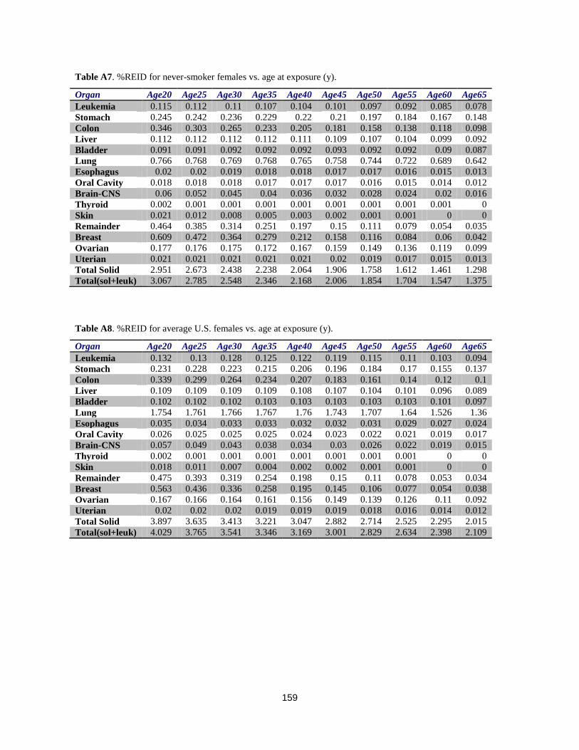
159

Table A8. %REID for average U.S. females vs. age at exposure (y).


Leukemia 0.132 0.13 0.128 0.125 0.122 0.119 0.115 0.11 0.103 0.094

Stomach 0.231 0.228 0.223 0.215 0.206 0.196 0.184 0.17 0.155 0.137

Colon 0.339 0.299 0.264 0.234 0.207 0.183 0.161 0.14 0.12 0.1

Liver 0.109 0.109 0.109 0.109 0.108 0.107 0.104 0.101 0.096 0.089

Bladder 0.102 0.102 0.102 0.103 0.103 0.103 0.103 0.103 0.101 0.097

Lung 1.754 1.761 1.766 1.767 1.76 1.743 1.707 1.64 1.526 1.36

Esophagus 0.035 0.034 0.033 0.033 0.032 0.032 0.031 0.029 0.027 0.024

Oral Cavity 0.026 0.025 0.025 0.025 0.024 0.023 0.022 0.021 0.019 0.017

Brain-CNS 0.057 0.049 0.043 0.038 0.034 0.03 0.026 0.022 0.019 0.015

Thyroid 0.002 0.001 0.001 0.001 0.001 0.001 0.001 0.001 0 0

Skin 0.018 0.011 0.007 0.004 0.002 0.002 0.001 0.001 0 0

Remainder 0.475 0.393 0.319 0.254 0.198 0.15 0.11 0.078 0.053 0.034

Breast 0.563 0.436 0.336 0.258 0.195 0.145 0.106 0.077 0.054 0.038

Ovarian 0.167 0.166 0.164 0.161 0.156 0.149 0.139 0.126 0.11 0.092

Uterian 0.02 0.02 0.02 0.019 0.019 0.019 0.018 0.016 0.014 0.012

Total Solid 3.897 3.635 3.413 3.221 3.047 2.882 2.714 2.525 2.295 2.015

Total(sol+leuk) 4.029 3.765 3.541 3.346 3.169 3.001 2.829 2.634 2.398 2.109

Table A7. %REID for never-smoker females vs. age at exposure (y).


Leukemia 0.115 0.112 0.11 0.107 0.104 0.101 0.097 0.092 0.085 0.078

Stomach 0.245 0.242 0.236 0.229 0.22 0.21 0.197 0.184 0.167 0.148

Colon 0.346 0.303 0.265 0.233 0.205 0.181 0.158 0.138 0.118 0.098

Liver 0.112 0.112 0.112 0.112 0.111 0.109 0.107 0.104 0.099 0.092

Bladder 0.091 0.091 0.092 0.092 0.092 0.093 0.092 0.092 0.09 0.087

Lung 0.766 0.768 0.769 0.768 0.765 0.758 0.744 0.722 0.689 0.642

Esophagus 0.02 0.02 0.019 0.018 0.018 0.017 0.017 0.016 0.015 0.013

Oral Cavity 0.018 0.018 0.018 0.017 0.017 0.017 0.016 0.015 0.014 0.012

Brain-CNS 0.06 0.052 0.045 0.04 0.036 0.032 0.028 0.024 0.02 0.016

Thyroid 0.002 0.001 0.001 0.001 0.001 0.001 0.001 0.001 0.001 0

Skin 0.021 0.012 0.008 0.005 0.003 0.002 0.001 0.001 0 0

Remainder 0.464 0.385 0.314 0.251 0.197 0.15 0.111 0.079 0.054 0.035

Breast 0.609 0.472 0.364 0.279 0.212 0.158 0.116 0.084 0.06 0.042

Ovarian 0.177 0.176 0.175 0.172 0.167 0.159 0.149 0.136 0.119 0.099

Uterian 0.021 0.021 0.021 0.021 0.021 0.02 0.019 0.017 0.015 0.013

Total Solid 2.951 2.673 2.438 2.238 2.064 1.906 1.758 1.612 1.461 1.298

Total(sol+leuk) 3.067 2.785 2.548 2.346 2.168 2.006 1.854 1.704 1.547 1.375

160

Appendix B Using the methods described in the text, risk calculations were made for each U.S. state and the District of Columbia using the NCRP No. 132 Model (as described in the text) and the BEIR VII model. The following tables show REID results for females and males at ages of exposure of 35, 45, and 55 y. The median life span and age-adjusted cancer mortality rate are also shown

161

Table B1. REID per Sv for males at different ages at exposure in NCRP and BEIR VII models.

State Median lifespan Cancer rate 35 45 55 35 45 55

Utah 80.2 96.0 3.78 3.69 3.46 3.69 2.85 1.95

North Dakota 79.2 103.8 3.98 3.86 3.64 3.96 3.03 2.05

Colorado 79.7 107.4 3.90 3.80 3.57 3.86 2.97 2.02

Wyoming 78.3 108.2 3.84 3.76 3.54 3.78 2.91 1.96

Alaska 78.4 112.8 4.03 3.93 3.69 4.08 3.13 2.14

Montana 78.5 113.5 3.92 3.85 3.66 3.88 2.97 2.02

Minnesota 80.1 115.0 4.18 4.06 3.84 4.09 3.12 2.11

Idaho 79.2 118.1 4.01 3.90 3.74 3.89 2.98 2.03

Connecticut 79.4 120.8 4.09 3.99 3.75 4.07 3.10 2.10

California 79.4 123.0 3.92 3.81 3.57 3.91 3.00 2.05

Vermont 79.6 123.9 4.08 3.94 3.73 4.02 3.06 2.06

Nebraska 79.0 125.8 3.96 3.85 3.59 3.90 2.96 1.99

New Mexico 78.1 126.0 3.76 3.69 3.48 3.76 2.91 2.01

Washington 79.3 126.5 4.06 3.95 3.73 3.99 3.04 2.07

New Hampshire 79.4 129.1 4.14 4.01 3.76 4.11 3.12 2.10

Wisconsin 78.9 130.6 4.10 3.99 3.76 3.99 3.03 2.04

New Jersey 78.7 132.7 3.99 3.88 3.65 3.97 3.02 2.04

Arizona 78.7 134.2 3.85 3.76 3.55 3.89 2.99 2.06

South Dakota 78.6 135.0 4.03 3.93 3.70 3.96 3.02 2.04

Oregon 78.8 135.9 3.98 3.87 3.63 3.95 3.01 2.04

Iowa 78.9 140.4 4.12 4.01 3.78 3.99 3.02 2.04

Nevada 76.5 140.4 3.70 3.61 3.40 3.68 2.80 1.91

Massachusetts 79.0 141.0 4.06 3.94 3.70 4.06 3.08 2.09

New York 79.1 141.5 3.96 3.84 3.60 3.92 2.99 2.03

Hawaii 80.3 144.5 3.91 3.76 3.53 3.99 3.07 2.11

Kansas 78.2 144.9 3.95 3.84 3.61 3.86 2.93 1.98

Texas 77.4 149.1 3.84 3.73 3.50 3.80 2.89 1.95

Maryland 77.7 150.2 3.89 3.78 3.55 3.90 2.97 2.02

Virginia 77.9 150.6 3.94 3.81 3.55 3.93 2.97 2.00

Illinois 77.8 151.2 3.99 3.88 3.65 3.92 2.97 2.00

Rhode Island 78.5 152.7 4.00 3.86 3.57 4.04 3.06 2.07

Michigan 77.7 157.0 3.90 3.79 3.56 3.84 2.91 1.97

Pennsylvania 77.3 158.8 3.91 3.80 3.56 3.86 2.92 1.96

Indiana 76.8 158.9 3.89 3.79 3.55 3.83 2.89 1.94

Maine 78.3 165.3 4.11 3.98 3.72 4.03 3.04 2.04

Ohio 76.9 168.3 3.87 3.76 3.52 3.83 2.88 1.94

Georgia 76.1 169.1 3.70 3.58 3.34 3.70 2.79 1.88

Delaware 77.4 170.9 3.97 3.88 3.63 3.96 3.00 2.03

Missouri 76.7 171.5 3.88 3.78 3.54 3.81 2.88 1.94

Florida 78.4 174.1 3.99 3.88 3.67 3.95 3.02 2.08

North Carolina 76.5 175.1 3.80 3.68 3.44 3.78 2.85 1.92

Kentucky 75.2 185.1 3.80 3.69 3.45 3.79 2.86 1.91

West Virginia 75.3 185.2 3.69 3.59 3.32 3.66 2.77 1.85

Oklahoma 75.4 187.5 3.66 3.56 3.34 3.60 2.72 1.82

South Carolina 75.5 196.2 3.77 3.66 3.45 3.74 2.82 1.91

Alabama 74.6 196.2 3.64 3.53 3.30 3.63 2.73 1.84

Tennessee 75.2 196.7 3.74 3.64 3.43 3.70 2.79 1.88

Arkansas 75.4 202.0 3.82 3.71 3.49 3.75 2.83 1.91

District of Columbia 73.2 205.0 3.48 3.41 3.29 3.56 2.72 1.90

Louisiana 74.2 212.3 3.67 3.57 3.34 3.68 2.77 1.87

Mississippi 73.7 219.0 3.59 3.49 3.27 3.59 2.70 1.81

BEIR VII NCRP 132

162

Table B2. REID per Sv for females at different ages at exposure in NCRP and BEIR VII models.

State Median lifespan Cancer rate 35 45 55 35 45 55

Alaska 82.6 89.6 5.43 5.26 4.85 4.82 3.62 2.42

Utah 83.1 99.4 4.84 4.64 4.21 4.27 3.22 2.13

Colorado 83.1 108.6 5.34 5.14 4.72 4.72 3.52 2.34

North Dakota 84.0 109.6 5.60 5.40 4.92 4.98 3.72 2.46

Idaho 83.0 111.5 5.45 5.25 4.86 4.71 3.52 2.33

Nebraska 83.2 114.3 5.47 5.27 4.84 4.80 3.58 2.37

Hawaii 85.6 114.4 5.46 5.22 4.76 4.93 3.73 2.50

Minnesota 84.0 117.1 5.74 5.54 5.09 5.04 3.76 2.49

Montana 82.8 117.5 5.50 5.32 4.91 4.85 3.62 2.40

Oregon 82.5 119.7 5.52 5.32 4.87 4.89 3.63 2.40

Connecticut 83.6 120.6 5.69 5.48 5.03 5.05 3.76 2.49

Washington 82.9 120.8 5.58 5.38 4.94 4.94 3.67 2.44

Wyoming 82.2 121.1 5.33 5.16 4.73 4.68 3.50 2.32

California 83.4 123.8 5.46 5.25 4.80 4.84 3.61 2.40

Maine 82.3 123.9 5.65 5.44 4.97 4.97 3.68 2.41

Wisconsin 83.3 126.0 5.61 5.40 4.95 4.91 3.65 2.41

Arizona 83.4 126.3 5.33 5.13 4.70 4.72 3.54 2.36

Vermont 83.3 127.4 5.53 5.31 4.83 4.89 3.63 2.39

New Mexico 83.1 127.5 5.25 5.05 4.62 4.67 3.50 2.33

Texas 82.2 128.8 5.18 4.96 4.52 4.56 3.39 2.24

Massachusetts 83.2 129.0 5.66 5.44 4.98 5.01 3.72 2.45

New Hampshire 83.1 129.2 5.64 5.39 4.92 5.01 3.71 2.45

Nevada 81.5 129.8 5.32 5.13 4.69 4.73 3.51 2.32

South Dakota 83.6 130.2 5.59 5.39 4.92 4.91 3.67 2.43

Rhode Island 83.0 130.7 5.64 5.44 5.00 4.92 3.65 2.41

Iowa 83.4 131.7 5.62 5.41 4.94 4.90 3.65 2.41

Virginia 82.2 135.2 5.37 5.14 4.67 4.74 3.51 2.31

New York 83.3 135.6 5.51 5.29 4.82 4.88 3.63 2.40

New Jersey 82.8 135.6 5.64 5.43 4.96 4.98 3.70 2.44

Kansas 82.4 135.9 5.36 5.15 4.71 4.68 3.48 2.30

Michigan 82.0 138.6 5.37 5.16 4.72 4.70 3.48 2.30

Illinois 82.4 139.5 5.50 5.28 4.82 4.84 3.58 2.36

Maryland 82.2 140.6 5.42 5.20 4.75 4.80 3.56 2.35

Pennsylvania 82.2 140.6 5.46 5.25 4.77 4.81 3.56 2.35

Georgia 81.2 142.7 5.07 4.85 4.41 4.43 3.28 2.16

North Carolina 81.7 143.6 5.18 4.96 4.51 4.56 3.39 2.23

Indiana 81.6 143.7 5.38 5.15 4.68 4.72 3.49 2.29

Missouri 81.7 145.3 5.34 5.12 4.65 4.69 3.47 2.28

Oklahoma 80.7 146.4 5.02 4.81 4.36 4.39 3.25 2.14

Florida 83.7 146.4 5.50 5.29 4.85 4.86 3.64 2.43

Ohio 81.5 147.2 5.36 5.14 4.67 4.70 3.47 2.28

Delaware 82.2 150.0 5.54 5.33 4.85 4.84 3.59 2.37

Alabama 80.5 152.2 4.97 4.77 4.33 4.33 3.21 2.11

West Virginia 80.4 153.1 5.21 5.01 4.54 4.56 3.36 2.19

South Carolina 81.3 154.0 5.11 4.88 4.44 4.50 3.34 2.21

Kentucky 80.8 156.9 5.34 5.13 4.62 4.66 3.43 2.24

Tennessee 80.8 158.6 5.15 4.93 4.48 4.52 3.34 2.20

Louisiana 80.1 161.7 5.10 4.87 4.42 4.48 3.31 2.17

Arkansas 81.3 163.5 5.24 5.02 4.56 4.58 3.39 2.23

Mississippi 80.4 165.1 5.04 4.82 4.38 4.36 3.23 2.13

District of Columbia 81.6 165.6 5.22 5.05 4.72 4.58 3.44 2.33

BEIR VII NCRP 132

163

The CDC101 has published life-table and cancer mortality rates for different levels of urbanization. We applied these rates using the NCRP No. 132 model with the LSS report solid cancer (DDREF=2) and the BEIR VII model (DDREF=1.5) to study age and gender dependence of REID values (Figures B1 and B2) for different locality as described by the CDC.

Figure B2. %REID per Sv for males and females in NCRP6 model with vT=0.5.

Figure B1. %REID per Sv for males and females in BEIR VII model with vT=0.5.

REPORT DOCUMENTATION PAGE Form Approved OMB No. 0704-0188

Public reporting burden for this collection of information is estimated to average 1 hour per response, including the time for reviewing instructions, searching existing data sources, gathering and

maintaining the data needed, and completing and reviewing the collection of information. Send comments regarding this burden estimate or any other aspect of this collection of information, including

suggestions for reducing this burden, to Washington Headquarters Services, Directorate for Information Operations and Reports, 1215 Jefferson Davis Highway, Suite 1204, Arlington, VA 22202-4302,

and to the Office of Management and Budget, Paperwork Reduction Project (0704-0188), Washington, DC 20503.

1. AGENCY USE ONLY (Leave Blank) 2. REPORT DATE 3. REPORT TYPE AND DATES COVERED

January 2013 Technical Publication

4. TITLE AND SUBTITLE

5. FUNDING NUMBERS

Space Radiation Cancer Risk Projections and Uncertainties – 2012

6. AUTHOR(S) Francis A. Cucinotta,* Myung-Hee Y. Kim,** Lori J. Chappell**

7. PERFORMING ORGANIZATION NAME(S) AND ADDRESS(ES) 8. PERFORMING ORGANIZATION REPORT NUMBERS

Lyndon B. Johnson Space Center

Houston, Texas 77058

S-1137

9. SPONSORING/MONITORING AGENCY NAME(S) AND ADDRESS(ES) 10. SPONSORING/MONITORING

AGENCY REPORT NUMBER

National Aeronautics and Space Administration

Washington, DC 20546-0001

TP-2012-217375

11. SUPPLEMENTARY NOTES

*NASA Johnson Space Center, Houston; **U.S.R.A., Division of Space Life Sciences, Houston

12a. DISTRIBUTION/AVAILABILITY STATEMENT 12b. DISTRIBUTION CODE

Unclassified/Unlimited Available from the NASA Center for AeroSpace Information (CASI) 7115 Standard Hanover, MD 21076-1320 Category: 52

13. ABSTRACT (Maximum 200 words)

Uncertainties in estimating health risks from galactic cosmic rays are a major limitation to the length of space missions and the

evaluation of potential risk mitigations. NASA limits astronaut exposures to a 3% risk of exposure-induced death and protects against

uncertainties in risks projections using an assessment of 95% confidence intervals in the projection model. Revisions to the NASA

projection model for lifetime cancer risks from space radiation and new estimates of model uncertainties are described. Our report

reviews models of space environments and transport code predictions of organ exposures, and characterizes uncertainties. We

summarize recent analysis of low linear energy transfer radio-epidemiology data, including revision to the Japanese A-bomb survivor

dosimetry, longer follow-up of exposed cohorts, and reassessments of dose and dose-rate reduction effectiveness factors. We compare

newer projections and uncertainties with earlier estimates. Current understanding of radiation quality effects and recent data on factors

of relative biological effectiveness and particle track structure are reviewed. Results from radiobiology experiments provide new

information on solid cancer and leukemia risks from heavy ions; radiation quality effects are described. New findings and knowledge

are used to revise the NASA risk projection model for space radiation cancer risks.

14. SUBJECT TERMS 15. NUMBER OF

PAGES

16. PRICE CODE

radiation effects; biological effects; radiation exposure; radiation hazards; radiation

injuries; radiation protection; radiation sickness; radiation tolerance; human tolerance 186

17. SECURITY CLASSIFICATION

OF REPORT


OF THIS PAGE


OF ABSTRACT

20. LIMITATION OF ABSTRACT

Unclassified Unclassified Unclassified Unlimited

Standard Form 298 (Rev Feb 89) (MS Word Mar 97) Prescribed by ANSI Std. 239-18 298-102

NSN 7540-01-280-5500

space radiation cancer risk projections and … space radiation cancer risk projections and...

Documents