Sovereign Debt and Structural Reforms�

Andreas Müllery Kjetil Storeslettenz Fabrizio Zilibottix

September 11, 2016

Abstract

Motivated by the European debt crisis, we construct a tractable theory of sovereign debt andstructural reforms under limited commitment. A sovereign country which has fallen into a recessionof an uncertain duration issues one-period debt to smooth consumption. It can also implementstructural policy reforms to speed up recovery from the recession. The sovereign can renege onits debt obligations by su¤ering an observable stochastic default cost, in which case creditors o¤era take-it-or-leave-it debt haircut to avert default. The laissez-faire Markov equilibrium featureslarge �uctuations in consumption, debt, and reform e¤ort. During the recession, consumption fallswhenever debt is honored. A large debt destroys incentives for structural reforms since some ofthe gains from reform accrue to the lenders. Allowing for �nancial markets with state-contingentdebt provides only limited consumption insurance. We contrast the Markov equilibrium with anoptimal contract with one-sided commitment. This allocation, which features step-wise increasingconsumption and step-wise decreasing reform e¤ort, can be interpreted as a �exible assistanceprogram provided by an international institution with commitment. We calibrate the model andshow that it can match a number of key stylized facts about debt and debt crises. We quantify thee¤ect of relaxing di¤erent contractual and �nancial frictions.JEL Codes: E62, F33, F34, F53, H12, H63Keywords: Austerity, Debt overhang, Default, European debt crisis, Fiscal policy, Great Re-

cession, Limited commitment, Markov equilibrium, Moral hazard, Renegotiation, Risk premia, Risksharing, Sovereign debt, Structural reforms.

�We would like to thank Manuel Amador, George-Marios Angeletos, Cristina Arellano, Marco Bassetto, TobiasBroer, Fernando Broner, Alessandro Dovis, Jonathan Eaton, Patrick Kehoe, Enrique Mendoza, Juan-Pablo Nicolini,Ugo Panizza, Aleh Tsyvinski, Jaume Ventura, Christopher Winter, Tim Worrall, and seminar participants at AnnualMeeting of the Swiss Society of Economics and Statistics, Barcelona GSE Summer Forum, Brown University, CEMFI,Columbia University, CREi, EIEF Political Economy Workshop, ESSIM 2016, European University Institute, GoetheUniversity Frankfurt, Graduate Institute of Geneva, Humboldt University, Istanbul School of Central Banking, NOR-MAC, Oxford, Royal Holloway, Swiss National Bank, Università Cà Foscari, Universitat Autonoma Barcelona, UniversityCollege London, University of Cambridge, University of Konstanz, University of Oslo, University of Oxford, Universityof Pennsylvania, University of Padua, University of Toronto, University of Zurich, and Yale University. We acknowledgesupport from the European Research Council (ERC Advanced Grant IPCDP-324085).

yUniversity of Oslo, Department of Economics, andreas.mueller@econ.uio.no.zUniversity of Oslo, Department of Economics, kjetil.storesletten@econ.uio.no.xUniversity of Zurich, Department of Economics, fabrizio.zilibotti@econ.uzh.ch.

1 Introduction

Sovereign debt crises and economic reforms have been salient intertwined policy issues throughoutthe Great Recession, especially in Europe. Economic theory o¤ers two simple policy prescriptions forcountries su¤ering a temporary decline in output. First, they should borrow on international marketsto smooth consumption. Second, they should undertake reforms �possibly painful in the short run�to speed up economic recovery. However, these simple policy prescriptions run into di¢ culties inthe presence of limited enforcement issues. On the one hand, risk sharing may be hampered by risingdefault premia associated with the risk of debt renegotiations.1 On the other hand, a large debt canreduce the borrower�s incentive to undertake economic reforms to boost economic growth since someof the gains from growth would accrue to the lenders.

To cast light on these trade-o¤s and to derive positive and normative predictions, this paper pro-poses a dynamic theory of sovereign debt that rests on four building blocks. The �rst is that sovereigndebt is subject to limited enforcement, and that countries can renege on their obligations subject toreal costs, as in e.g. Aguiar and Gopinath (2006), Arellano (2008) and Yue (2010). Departing from theprevious literature, we assume the size of default costs to be stochastic, re�ecting exogenous changesin the domestic and international situation. The second building block is that whenever creditors facea credible default threat, they can make a take-it-or-leave-it renegotiation o¤er to the indebted coun-try. This approach conforms with the empirical observations that unordered defaults are rare events,and that there is great heterogeneity in the terms at which debt is renegotiated, as documented byTomz and Wright (2007) and Sturzenegger and Zettelmeyer (2008). The third building block is thepossibility for the government of the indebted country to make structural policy reforms that speedup recovery from an existing recession. Examples of such reforms include labor and product marketderegulation, and the establishment of �scal capacity that allows the government to raise tax revenuee¢ ciently (see, e.g., Ilzkovitz and Dierx 2011). While these reforms are bene�cial in the long run,they may entail short-run costs for citizens at large, governments or special-interest groups (see, e.g.,Blanchard and Giavazzi 2003, and Boeri 2005). The fourth building block is the assumption that mar-kets �nd it di¢ cult to coordinate punishment for past bad behavior of governments. More precisely,markets charge a high interest rate on highly indebted countries, but have no additional instrument todiscipline, ex-post, non-virtuous governments. This idea is captured by the notion of a Markov-perfectequilibrium, which excludes reputational mechanisms.

More formally, we construct a dynamic model of an endowment economy subject to income shocksfollowing a two-state Markov process. A benevolent local government can issue sovereign debt tosmooth consumption. The country starts in a recession of an unknown duration. The probabilitythat the recession ends is endogenous, and hinges on the government�s reform e¤ort. Debt issuance issubject to a limited-commitment problem: the government can, ex-post, repudiate its debt, based onthe publicly observable realization of a stochastic default cost. When this realization is su¢ ciently lowrelative to the outstanding debt, the default threat is credible. In this case, a syndicate of creditorsmakes a take-it-or-leave-it debt haircut o¤er, as in Bulow and Rogo¤ (1989). In equilibrium, there isno outright default, but debt renegotiations. Haircuts are more frequent during recession, and morefrequent the larger is the outstanding sovereign debt. Consumption increases after a renegotiation, in

1Greece, the hardest hit country in Europe, saw its debt-GDP ratio soar from 107% in 2008 to 170% in 2011, atwhich point creditors had to agree to a debt haircut implying a 53% loss on its face value. Meanwhile, internationalorganizations stepped in to provide �nancial assistance and access to new loans, asking in exchange �scal austerity and acommitment to economic reforms. A new crisis with a request from the Greek government of a haircut on the outstandingdebt was barely averted in the summer of 2015.

1

line with the empirical evidence that economic conditions improve in the aftermath of debt relief, asdocumented in Reinhart and Trebesch (2016).

We �rst characterize the laissez-faire equilibrium. During recessions, the government would liketo issue debt in order to smooth consumption. However, as debt accumulates, the probability ofrenegotiation increases, implying a rising risk premium and consumption volatility. The reform e¤ortexhibits a non-monotonic pattern: it is increasing with debt at low levels of debt because of thedisciplining e¤ect of recession. However, for su¢ ciently high debt levels the relationship is �ippedbecause of a debt overhang problem: very high debt levels deter useful reforms because most of thegains from the reforms accrue to foreign lenders in the form of capital gains on the outstanding debt.The moral hazard problem exacerbates the country�s inability to achieve consumption smoothing: athigh debt levels, creditors expect little reform e¤ort, are pessimistic about the economic outlook, andrequest an even higher risk premium. We also consider an economy in which the government can issuedebt whose payment is contingent on the stochastic realization of the endowment. We show that evenin this case, the moral hazard in reform e¤ort prevents full insurance.2

Next, we characterize the dynamic principal-agent problem when the planner, contrary to investorsin the competitive equilibrium, can commit to punish the agent (i.e., the sovereign government) whenshe deviates from the optimal contract. However, the enforcement power is limited: the agent to quitpermanently the contract and resort to the competitive (Markov) equilibrium after paying the defaultcost. When this happens (out of equilibrium), the planner can exclude permanently the agent fromfuture contractual relations. In other words, the agent can bene�t from the principal�s commitmentpower that the market lacks. However, there is only one opportunity to be in the contract. If theagent quits, it is for good. We consider two alternative cases. In the �rst, the planner can observe(as do investors in the competitive equilibrium) the reform e¤ort. In the second, the planner cannotobserve it. The optimal contract with observable e¤ort is very di¤erent from the market equilibrium:it features non-decreasing consumption and non-increasing reform e¤ort during the recession. Moreprecisely, consumption and e¤ort remain constant whenever the country�s participation constraint isnot binding. However, when the constraint is binding the planner increases the country�s promisedutility and consumption, and reduces the required reform e¤ort. In contrast, the optimal contract withunobservable e¤ort is identical to the market equilibrium where investor can observe the reform e¤ortbut cannot commit to punish deviations and where the sovereign government can issue state-contingentdebt.

We provide an institutional interpretation of the optimal contract. The optimal contract can beinterpreted as the intervention of an independent institution (e.g., the IMF) that can provide assistanceto the economy in recession, and that commits to abandon its assistance program if the country doesnot implement the required reforms, assumed to be ex-post observable. During the recession theoptimal program entails a persistent budget support through extending loans on favorable terms,combined with a larger reform e¤ort than the borrower would choose on its own. Upon recovery fromthe recession, the sovereign government is settled with a (large) debt on market terms. A commonobjection to schemes implying deferred repayment is that the country may refuse to repay its loanswhen the economy recovers. In our theory, this risks is factored in as part of the contract. The optimal

2 In standard models without moral hazard, state-contingent debt would provide insurance against the continuationof a recession �i.e., Arrow securities paying o¤ conditional on the aggregate state, recession or normal times. However,the better insured the country is, the more severe the moral hazard problem becomes. For instance, full insurance wouldremove incentives to exert reform e¤ort. Since this is priced into the debt, the social value of state-contingent debt islimited. In a calibrated version of the model, we show that state-contingent debt yields very small welfare gains relativeto the equilibrium with non-state contingent debt.

2

program has the interesting feature that, whenever the country can credibly threaten to default, theinternational institution should relent and improve the terms of the agreement for the debtor bygranting her higher consumption and a lower reform e¤ort. In other words, the austerity program isrelaxed over time, whenever necessary to avert the breakdown of the program.

We provide a quantitative evaluation of the theory with the aid of a calibrated version of the model.The model matches realistic debt-to-GDP ratios, as well as default premia, renegotiation frequencies,and recovery rates. We regard this as a contribution in itself. In the existing quantitative literature,it is di¢ cult to sustain high debt levels, contrary both to the observation that many countries havemanaged to �nance debt-GDP ratios above 100%, and to the estimates of a recent study by Collard,Habib, and Rochet (2015) showing that OECD countries can sustain debt-GDP ratios even in excessof 200%. We �nd that an assistance program implementing the constrained optimum yields largewelfare gains, equivalent to a transfer of 45% of the initial GDP with a zero expected cost for theinstitution running the assistance program.

1.1 Literature review

Our paper relates to several streams of the literature on sovereign debt. By focusing on Markovequilibria, we abstract from reputational mechanisms, being close in the spirit to the direct-punishmentapproach proposed by Bulow and Rogo¤ (1989).3 Our work is related to the more recent quantitativemodels of sovereign default such as Aguiar and Gopinath (2006) and Arellano (2008). Yue (2010)considers, as we do, the possibility of renegotiation, although in her model renegotiation is costly andis determined by Nash bargaining between creditors and debtors - with no stochastic shocks to outsideoptions. In her model, ex-post ine¢ cient restructuring helps ex-ante discipline and provides incentivesto honor the debt.4 This literature does not consider the e¢ cient allocation nor economic reforms.Moreover, we pursue an analytical characterization of the properties of the model, whereas the mainfocus of this literature has been quantitative.

In terms of reform e¤ort, our paper is related to Krugman (1988), Atkeson (1991) and Jeanne(2009). Krugman (1988) showed that when a borrower has a large debt, productive investmentsmight not be undertaken (the �debt overhang�). His is a static model where debt is exogenous.Atkeson (1991) studies the optimal contract in an environment in which an in�nitely-lived borrowerfaces a sequence of two-period lived lenders. The borrower can use funds to invest in productivefuture capacity or to consume the funds. However, the lenders cannot observe the allocation toinvestment or consumption. Our paper di¤ers from Atkeson�s in various aspects. First, in our modelwe focus on Markov equilibria where the borrower cannot commit the reform e¤ort, but the lendercan observe it. This seems a plausible abstraction in the context of, for example, the European debtcrisis. Second, in the COA, the planner can observe the e¤ort, but its power to punish deviations islimited by the ability of the sovereign to revert to the competitive (Markov) equilibrium. Third, in ourtheory structural reforms a¤ect the future stochastic process of income, while his model investmentsonly a¤ect next period�s income. Finally, in our model all agents (and the planner) have an in�nitehorizon. The results are di¤erent. Atkeson (1991) shows that the optimal contract involves capital

3The distinction between the reputation approach and the punishment approach as the two main conceptual frame-works in the literature on sovereign debt crisis has been introduced recently by Bulow and Rogo¤ (2015).Pioneer contributions to the analysis of debt repudiation based on reputational mechanisms such as the threat of future

exclusion from credit markets include Eaton and Gersovitz (1981), Grossman and Van Huyck (1988), and Fernandez andRosenthal (1989).

4Other papers focusing on the restructuring of sovereign debt include Asonuma and Trebesch (2016), Benjamin andWright (2009), Bolton and Jeanne (2007), Dovis (2016), and Mendoza and Yue (2012).

3

out�ow from the borrower during the worst aggregate state. Our model predicts instead that in arecession the borrower keeps accumulating debt and renegotiates it periodically. Moreover, in ourmodel the constrained optimal allocation (though not necessarily the competitive equilibrium) hasnon-decreasing consumption when reform e¤ort is observable. Jeanne (2009) studies an economywhere the government takes a policy action that a¤ects the return to foreign investors (e.g., theenforcement of creditor�s right) but this can be reversed within a time horizon that is shorter thanthat at which investors must commit their resources.

Dovis (2016) studies the e¢ cient risk-sharing arrangement between a sovereign borrower withlimited commitment and international lenders in a framework with informational frictions. He showsthat the e¢ cient allocation can be implemented with non-contingent defaultable bonds of short andlong maturity. In his framework, ex post ine¢ cient outcomes (i.e., sovereign default episodes) arenecessary to support the e¢ cient allocation. We focus instead on a decentralized Markov equilibriumwhere international markets lack the commitment to coordinate on ex post ine¢ cient punishments,and emphasize the interaction between structural reforms and limited commitment. Instead, ex poste¢ cient renegotiations of debt contracts are observed in equilibrium whenever the sovereign defaultthreat is credible.

Hopenhayn and Werning (2008) study the optimal corporate debt contract between a bank and arisk-neutral borrowing �rm. As we do, they assume that the borrower has a stochastic default cost.Di¤erent from us, they focus on the case when this outside option is not observable to the lender andshow that this implies that default can occur in equilibrium. They do not study reform e¤ort nor dothey analyze the case of sovereign debt issued by a country in recession.

Another recent paper complementary to ours is Conesa and Kehoe (2015). In their theory, undersome circumstances, the government of the indebted country may opt to �gamble for redemption.�Namely, it runs an irresponsible �scal policy that sends the economy into the default zone if therecovery does not happen soon enough. The source and the mechanism of the crisis are di¤erentfrom ours. Their model is based on the framework of Cole and Kehoe (1996, 2000) inducing multipleequilibria and sunspots.

Our paper is related also to the literature on endogenous incomplete markets due to limited en-forcement or limited commitment. This includes Alvarez and Jermann (2000) and Kehoe and Perri(2002). The analysis of constrained e¢ ciency is related to the literature on competitive risk sharingcontracts with limited commitment, including Thomas and Worrall (1988), Kocherlakota (1996), andKrueger and Uhlig (2006). An application of this methodology to the optimal design of a FinancialStability Fund is provided by Abraham, Carceles-Poveda, and Marimon (2014). In our model all debtis held by foreign lenders. Recent papers by Broner, Martin, and Ventura (2010), Broner and Ventura(2011), and Brutti and Sauré (2016) study the implications for the incentives to default of havingpart of the government debt held by domestic residents. Song et al. (2012) and Müller et al. (2016)focus, as we do, on Markov equilibria to study the politico-economic determination of debt in openeconomies where governments are committed to honor their debt. An excellent review of the sovereigndebt literature is provided by Aguiar and Amador (2014).

In the large empirical literature, our paper is related to the �nding of Tomz and Wright (2007).Using a dataset for the period 1820�2004, they �nd a negative but weak relationship between economicoutput in the borrowing country and default on loans from private foreign creditors. While countriesdefault more often during recessions, there are many cases of default in good times and many instancesin which countries have maintained debt service during times of very bad macroeconomic conditions.They argue that these �ndings are at odds with the existing theories of international debt. Our theoryis consistent with the pattern they document. In our model, due to the stochastic default cost, countries

4

may default during booms (though this is less likely, consistent with the data) and can conversely failto renegotiate their debt during very bad times. Their �ndings are reinforced by Sturzenegger andZettelmeyer (2008) who document that even within a relatively short period (1998-2005) there are verylarge di¤erences between average investor losses across di¤erent episodes of debt restructuring. Theobservation of such a large variability in outcomes is in line with our theory, insofar as the bargainingoutcome hinges on an outside option that is subject to stochastic shocks. Borensztein and Panizza(2009) evaluate empirically the costs that may result from an international sovereign default, includingreputation costs, international trade exclusion, costs to the domestic economy through the �nancialsystem, and political costs to the authorities. They �nd that the economic costs are generally short-lived. Finally, the relationship between consumption and renegotiations is in line with the evidencedocumented by Reinhart and Trebesch (2016), as discussed above. For a thorough review of theevidence, see also Panizza et al. (2009).

The rest of the paper is organized as follows. Section 2 describes the model environment. Section 3characterizes the competitive Markov equilibrium. Section 4 solves for the optimal dynamic contractunder the assumption that the principal (creditors) has full commitment, whereas the agent (sovereigngovernment) is subject to limited commitment. A decentralized interpretation of the optimal contractis provided. Section 5 presents quantitative positive and normative implications of the theory withthe aid of a calibrated economy. Section 6 concludes. Two online appendixes contain, respectively, theproofs of the main propositions and lemmas (Appendix A) and additional technical material referredin the text (Appendix B).

2 The model environment

The model economy is a small open endowment economy populated by an in�nitely-lived representativeagent. The endowments follow a two-state Markov switching process, with realizations w 2 fw; �wg,where 0 < w < �w. We label the two endowment states, respectively, recession and normal times.Normal times is assumed to be an absorbing state. If the economy starts in a recession, it switchesto normal times with probability p and remains in the recession with probability 1� p. A benevolentgovernment (henceforth, the sovereign) can implement a costly reform policy to increase the probabilityof a recovery. In our notation, p is both the reform e¤ort and the probability that the recession ends.The assumption that normal times is an absorbing state aids tractability and enables us to obtainsharp analytical results. In Section 5, we generalize the model to the case of recurrent recessions.

The preferences of the representative agent are described by the following expected utility function:

E0X

�t�u (ct)� �tIfdefault in tg �X (pt)

�:

The utility function u is twice continuously di¤erentiable and satis�es limc!0 u(c) = �1, u0 (c) > 0, and u00 (c) < 0. I 2 f0; 1g is an indicator switching on when the economy is in a default stateand � is a stochastic default cost assumed to be i.i.d. over time and to be drawn from the p.d.f.f (�) with an associated c.d.f. F (�) :We assume that F (�) is continuously di¤erentiable everywhere,and denote its support by @ � [0; �max] � R+, where �max < 1. The assumption that shocks areindependent is inessential, but aids tractability. X is the cost of reform, assumed to be an increasingconvex function of the probability of exiting recession, p 2 [p; �p] � [0; 1]. X is assumed to be twicecontinuously di¤erentiable, with the properties that X

�p�= 0; X 0 (p) > 0 and X 00 (p) > 0. In normal

times, X = 0.

5

To establish a benchmark, we characterize the optimal allocation under full insurance and fullenforcement (labelled the �rst-best allocation). The economy is assumed to start with an outstandingobligation of b given an implicit gross rate of return of R = ��1. The �rst-best allocation entailsperfect insurance: the country enjoys a constant stream of consumption and exerts a constant reforme¤ort during recession (during normal times, there is no e¤ort). The level of b lowers consumptionand increases reform e¤ort in recession.

Proposition 1 Let WFB (b; w) ; cFB (b; w) and pFB (b) denote, respectively, the discounted utility,consumption and e¤ort as a function of the outstanding obligation b, with w 2 fw; �wg denoting theinitial state of productivity. Then, for an economy starting in normal state:

cFB (b; �w) = �w � (1� �) b; WFB (b; �w) =u�cFB (b; �w)

�1� � :

For an economy starting in recession:

cFB (b; w) =(1� �)w + �pFB (b) �w1� � (1� pFB (b)) � (1� �) b;

WFB (b; w) =u�cFB (b; w)

�1� � �

X�pFB (b)

�1� � (1� pFB (b))

where pFB (b) is the reform e¤ort exerted for as long as the economy stays in recession. pFB (b) is theunique solution for pFB satisfying the following condition:

�

1� � (1� pFB)

0B@ ( �w � w)� u0�cFB (b; w)

�| {z }increase in output if econ. recovers

+ X�pFB

�| {z }saved e¤ort cost if econ. recovers

1CA = X 0 �pFB� : (1)

Moreover, when e¤ort is interior, cFB (b; w) and pFB (b) are, respectively, decreasing and increasingfunctions of b.

3 Competitive equilibrium

In the competitive equilibrium, the sovereign can issue a one-period bond (sovereign debt) to smoothconsumption. The bond, b, is a claim to one unit of the next-period consumption good, which sellstoday at the price Q (b; w). Bonds are purchased by a representative risk neutral foreign creditor whohas access to an international risk-free portfolio paying the world interest rate R. For simplicity, wefocus on the case in which �R = 1, although our main insights carry over to the case in which �R < 1(see Section 5). After issuing debt, the country decides its reform e¤ort.

The key assumptions are that (i) the country cannot commit to repay its sovereign debt, and(ii) the reform e¤ort is not contractible. At the beginning of each period, the sovereign observesthe realization of the default cost �; and decides whether to repay the debt that reaches maturityor to announce default on all its debt. The cost � is publicly observed, and captures in a reducedform a variety of shocks including both taste shocks (e.g., the sentiments of the public opinion aboutdefaulting on foreign debt) and institutional shocks (e.g., the election of a new prime minister, a new

6

central bank governor taking o¢ ce, the attitude of foreign governments, etc.).5 If a country defaults,no debt is reimbursed.6

When the sovereign announces its intention to default, a syndicate of creditors can make a take-it-or-leave-it renegotiation o¤er that we assume to be binding for all creditors. By accepting therenegotiation o¤er, the sovereign averts the default cost. In equilibrium, a haircut is o¤ered onlyif the default threat is credible, i.e., if the realization of � is su¢ ciently low to make the countryprefer default to full repayment. When they o¤er renegotiation, creditors make the debtor indi¤erentbetween an outright default and the proposed haircut.

In summary, the timing is as follows: The sovereign enters the period with the pledged debt b,observes the realization of w and �, and then decides whether to announce default. If the threat iscredible, the creditors o¤er a haircut. Next, the country decides whether to accept or decline the o¤er.Then, the sovereign issues new debt subject to the period budget constraint Q�b0 = B (b; �; w)+c�w,where B (b; �; w) � b denotes the debt level after the renegotiation stage. For technical reasons we alsoimpose that debt is bounded, b 2 [b;~b] where b 2 (�1; 0] and ~b = �w= (R� 1) is the natural borrowingconstraint in normal times. In equilibrium, these bounds will never be binding. If the country couldcommit to honor its debt, it would sell bonds at the price Q = 1=R. However, due to the risk ofdefault or renegotiation, it sells at a discount, Q � 1=R. Next, consumption is realized, and �nallythe sovereign decides its reform e¤ort.

3.1 De�nition of Markov equilibrium

In the characterization of the competitive equilibrium, we restrict attention to Markov-perfect equi-libria where the set of equilibrium functions only depend on the pay-o¤ relevant state variables, b,�, and w. This rules out that the sovereign�s decisions can be a¤ected by the desire to establish ormaintain a reputation.

De�nition 1 A Markov-perfect equilibrium is a set of value functions fV;Wg, a threshold renegoti-ation function �, an equilibrium debt price function Q, a set of optimal decision rules fB; B; C;g,such that, conditional on the state vector (b; �; w) 2

�[b;~b]� [0; �max]� fw; �wg

�, the sovereign and

the international creditors maximize utility, and markets clear. More formally:

� The value function V satis�es

V (b; �; w) = max fW (b; w) ;W (0; w)� �g ; (2)

where W (b; w) is the value function conditional on the debt level b being honored,

W (b; w) = maxb02[b;~b]

u�Q�b0; w

�� b0 + w � b

�+ Z

�b0; w

�;

5Alternatively, � could be given a politico-economic interpretation, as re�ecting special interests of the groups inpower. For instance, the government may care about the cost of default to its constituency rather than to the populationat large. In the welfare analysis, we stick to the interpretation of a benevolent government and abstract from politico-economic factors, although the model could be extended in this direction.

6For simplicity, we assume that � captures all costs associated with default. In an earlier version of this paper, weassumed that the government could not issue new debt in the default period, but were allowed to start issuing bondsalready in the following period. The results are unchanged. One could even consider richer post-default dynamics, suchas prolonged or stochastic exclusion from debt markets. Since outright default does not occur in equilibrium, the detailsof the post-default dynamics are immaterial.

7

and where Z is de�ned as

Z�b0; w

�= max

p2[p;�p]

��X (p) + �

�p� E

�V�b0; �0; �w

��+ (1� p)� E

�V�b0; �0; w

���; (3)

Z�b0; �w

�= �E

�V�b0; �0; �w

��(4)

and E�V�x; �0; w

��=R@ V (x; �;w) dF (�).

� The threshold renegotiation function � satis�es

� (b; w) =W (0; w)�W (b; w) : (5)

� The debt price function satis�es the following arbitrage conditions:

Q (b; �w) = Q̂ (b; �w) (6)

Q (b; w) = (b)� Q̂ (b; �w) + [1�(b)]� Q̂ (b; w) (7)

where Q̂ (b; w) is the bond price conditional on next period being in state w,

Q̂ (b; w) � 1

R(1� F (� (b; w))) + 1

R

1

b

Z �(b;w)

0b̂ (�;w)� f (�) d�; (8)

and where b̂ (�;w) is the new debt after a renegotiation given a realization �. b̂ is implicitly

de�ned by the condition W�b̂ (�;w) ; w

�=W (0; w)� �:

� The set of optimal decision rules comprises:

1. A take-it-or-leave-it debt renegotiation o¤er:

B (b; �; w) =�b̂ (�;w) if � � � (b; w) ;b if � > � (b; w) :

(9)

2. An optimal debt accumulation and an associated consumption decision rule:

B (B (b; �; w) ; w) = arg maxb02[b;~b]

�u�Q�b0; w

�� b0 + w � B (b; �; w)

�+ Z

�b0; w

�; (10)

C (B (b; �; w) ; w) = Q (B (B (b; �; w) ; w) ; w)�B (B (b; �; w) ; w) + w � B (b; �; w) : (11)

3. An optimal e¤ort decision rule:

�b0�= arg max

p2[p;�p]

��X (p) + �

�p� E

�V�b0; �0; �w

��+ (1� p)� E

�V�b0; �0; w

���: (12)

� The equilibrium law of motion of debt is b0 = B (B (b; �; w) ; w) :

� The probability that the recession ends is p = (b0).

8

V and W denote the sovereign�s value functions. Equation (2) states that when � > � (b; w) thereis no renegotiation, otherwise the sovereign renegotiates its debt. Since, ex-post, creditors have all thebargaining power, the discounted utility accruing to the sovereign equals the value that she would getunder outright default. Thus,

V (b; �; w) =

�W (b; w) if b � b̂ (�;w) ;

W (0; w)� � if b > b̂ (�;w) :

Consider, next, the equilibrium debt price function. Since creditors are risk neutral, the expectedrate of return on the sovereign debt must equal the risk-free rate of return. Then, the arbitrageconditions (6)�(7) ensure market clearing in the bond market and pin down the equilibrium bondprice in normal times and recession, respectively. The function Q̂ de�ned in equation (8) yields thebond price after the state w has realized but before knowing �:With probability 1�F (� (b; w)) debtis honored, where � (b; w) denotes the threshold default shock realization such that, conditional onthe debt b; the sovereign cannot credibly threaten to default for all � � � (b; w). With probabilityF (� (b; w)), debt is renegotiated to a level that depends on the realization of �: This level is given byb̂ (�;w) which, recall, denotes the renegotiated debt level that keeps the sovereign indi¤erent betweenaccepting the creditors� o¤er and defaulting. In the rest of the paper, we use the more compactnotation EV (b; w) � E [V (b; �; w)] and EV (b0; w) � E

�V�b0; �0; w

��:

Consider, �nally, the set of decision rules. (9) stipulates that creditors always extract the entiresurplus at the renegotiation stage. Equations (10)-(11) yield the optimal consumption-saving decisionssubject to a resource constraint. Equation (12) yields the optimal e¤ort decision. Note that the e¤ortexerted depends on b0, since e¤ort is chosen after the new debt is issued.

3.2 Existence of a Markov equilibrium

The crux for proving the existence of a Markov equilibrium lies in establishing the existence of thevalue function W . Once this is done, all the equilibrium functions (V;�; b̂; Q; Z;B; B; C;) can bederived from the set of de�nitions above. Before proving the existence of W; we establish an intuitiveproperty linking b̂ and �:

Lemma 1 Suppose a value functionW (b; w) exists and is strictly decreasing in b. Then, b̂ (� (b; w) ; w) =b: Moreover, � (b; w) is strictly increasing in b, hence, b̂ (�; �w) = ���1 (�) and b̂ (�;w) = ��1 (�), where�� (b) � � (b; �w) ; and � (b) � � (b; w) :

The lemma follows from the de�nitions of b̂ and �. On the one hand, b̂ (�;w) is the debt level that,conditional on �, makes the debtor indi¤erent between honoring and defaulting. On the other hand,� (b; w) is the realization of � that, conditional on b, makes the debtor indi¤erent between honoringand defaulting.

The next proposition establishes the existence of a Markov equilibrium. The proof establishes thatthe value function W is a �xed-point of a monotone mapping following Theorem 17.7 in Stokey andLucas (1989).

Proposition 2 There exists a Markov equilibrium, i.e., a set of equilibrium functions (V;W;�; b̂; Q; Z;B; B; C;)satisfying De�nition 1. The value functions V and W are continuous and non-increasing in b. Theequilibrium functions �; Q and are also continuous in b: The bond revenue, Q(b; w)b, is non-decreasing in b: The policy function B (b; w) is non-decreasing in b.

9

Proposition 2 establishes the existence but not the uniqueness of the Markov equilibrium. Thecorollary of Theorem 17.7 in Stokey and Lucas (1989) provides a strategy to verify numerically whetheran equilibrium is unique. We state this as Corollary 1 in Appendix A.

The next proposition establishes local di¤erentiability properties of the value function W , andthat the �rst-order conditions are necessary. Due to the possibility that debt is renegotiated, thevalue functions are not necessarily concave. Nevertheless, we establish that the equilibrium functionsare di¤erentiable at all debt levels that can result from an optimal choice given some initial debt level.We de�ne formally the set of such debt levels as B(w) = fx 2 [b;~b] j B (b; w) = x; for some b 2 [b;~b]g.7

Proposition 3 The equilibrium functions W (b; w), Z(b; w); �(b; w), Q(b; w), (b) are di¤erentiablefor all b 2 B(w). Moreover, for any b0 2 B(w); the �rst-order condition (@=@b0)u (Q(b0; w)b0 + w � b)+(@=@b0)Z (b0; w) = 0 and the envelope condition @W (b0; w)=@b0 = �u0 (C (b0; w)) holds true.

The proof in Appendix A is an application of the envelope theorem of Clausen and Strub (2013)that applies to problems including endogenous functions such as default probabilities and interestrates (see also Arellano et al. 2014).

Hereafter, for simplicity, we refer to the competitive Markov equilibrium as the competitive equi-librium.

3.3 Competitive equilibrium in normal times

In this section, we characterize the equilibrium when the economy is in normal times (w = �w), inwhich case there is no aggregate uncertainty. The next lemma establishes properties of the debtrevenue function at the optimal interior debt choice.

Lemma 2 The debt revenue function Q(b0; �w)b0 is concave in b0 2 [b;~b] and di¤erentiable for allb0 2 B(w) where @ (Q (b0; �w) b0) =@b0 = R�1 (1� F (� (b0; �w))).

An immediate implication of the lemma is that if we de�ne �b to be the lowest debt inducingrenegotiation almost surely (i.e., such that limb0!�b F (�(b

0; �w)) = 1), then, �b is also the top of the

La¤er curve, i.e., the endogenous debt limit. More formally, �b � minnargmaxb2[b;~b] fQ (b; �w) bg

o< ~b:

Although the borrower could issue debt exceeding �b, the marginal debt revenue would be zero forb0 > �b since this debt would never be honored.

We now study the consumption and debt dynamics. We introduce a de�nition that will be usefulthroughout the paper.

De�nition 2 A Conditional Euler Equation (CEE) describes the (expected) marginal rate of substi-tution between current and next-period consumption in all states of nature �0 that induce the sovereignto honor its debt next period.

Next, we characterize formally the CEE. The sovereign solves the consumption-saving problemgiven by (10). The �rst-order condition and the envelope theorem yield the following proposition.

7We prove later that during normal times the equilibrium functions are di¤erentiable everywhere. However, this isnot true in recession. In this case Proposition 3 shows that di¤erentiability still holds for all b that can be attained asan optimal choice.

10

Proposition 4 If the realization of �0 induces no renegotiation, then the following CEE holds true:

�Ru0 (c0jH; �w)u0 (c)

= 1; (13)

where c = C (B (b; �; �w) ; �w) is current consumption and c0jH; �w = C (b0; �w) = C (B (B (b; �; �w) ; �w) ; �w)is next-period consumption conditional on no renegotiation. Since �R = 1; then b0 = B (b; �w) = b,and consumption remains constant. Moreover, for all b < �b, the value function W (b; �w) is strictlydecreasing, strictly concave and twice continuously di¤erentiable in b, and consumption C(b; �w) isstrictly falling in b.

Although the CEE (13) resembles a standard Euler equation under full commitment, the similarityis deceiving: R is not the ex-post interest rate when debt is fully honored; the realized interest rate isin fact higher due to the default premium.

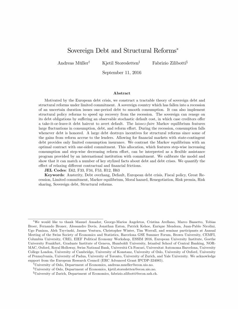
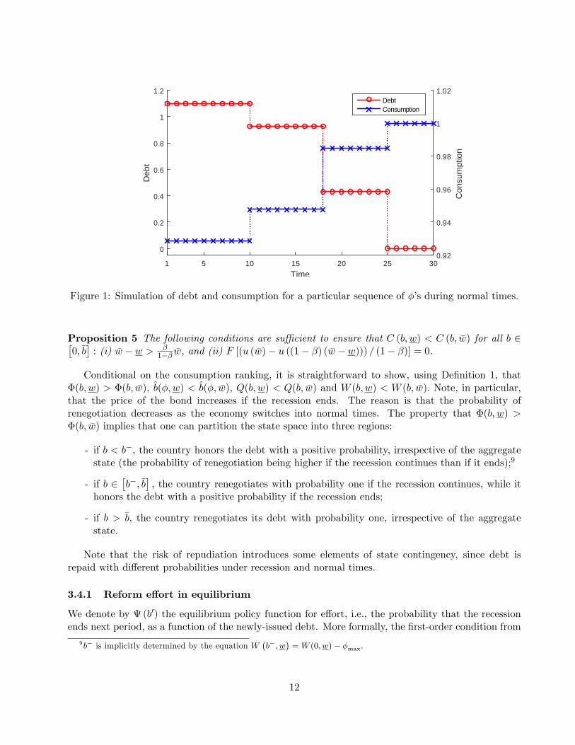
When debt is renegotiated, consumption increases discretely, hence u0 (ct) =u0 (ct+1) > �R. This isnot surprising, since the country bene�ts from a reduction in debt repayment.8 Thus, consumptionand debt are, respectively, increasing and decreasing step functions over time: they remain constantin every period in which the country honors its debt, while changing discretely upon every episodeof renegotiation. Figure 1 illustrates a simulation of the consumption and debt dynamics. Note thatthe sequence of renegotiations eventually brings the debt to a su¢ ciently low level where the riskof renegotiation vanishes. This consumption path is di¤erent from the �rst-best allocation whereconsumption and debt are constant for ever. Interestingly, in the long run, consumption is higher inthe competitive equilibrium with the risk of repudiation than in the �rst best allocation.

It is straightforward to generalize the results to the case of �R < 1 under the assumption thatutility features constant relative risk aversion. In this case, when the debt is honored debt wouldincrease and consumption would fall. After each episode of renegotiation the economy would startagain accumulating debt. In a world comprising economies with di¤erent �; e.g., some with �R = 1and some with �R < 1; economies with low � would experience recurrent debt crises.

3.4 Equilibrium under recession

When the economy is in recession the sovereign chooses, sequentially, whether to honor the currentdebt, how much new debt to issue, and how much reform e¤ort to exert. In this section, we assumethat the sovereign cannot issue state-contingent debt, i.e., securities whose payment is contingent onthe aggregate state of the economy. In Section 3.5 below we relax this restriction.

A natural property of the competitive equilibrium is that C (b; w) < C (b; �w) for all b � �b: con-ditional on honoring a giving debt level, consumption is higher in normal times than in a recession.Although we could �nd no numerical counterexample to this property, it is di¢ cult to prove it ingeneral because the equilibrium functions for consumption, e¤ort and debt price are determined si-multaneously. However, we can provide a su¢ cient condition in terms of the primitive parameters ofthe model.

8The prediction that whenever debt is renegotiated consumption increases permanently is extreme, and hinges on theassumptions that �R = 1 and that � is i.i.d. with a known distribution. In Section B.3 of Appendix B we extend themodel to a setting where there is uncertainty about the true distribution of � and the market learns about this distributionby observing the sequence of ��s. In this case, a low realization of � has two opposing e¤ects on consumption: on theone hand, a low � triggers debt renegotiation which on its own would increase consumption; on the other hand, a low �a¤ects the beliefs about the distribution of �, inducing the market to regard the country as less creditworthy (namely,the country draws from a distribution where low � is more likely). This tends to increase the default premium on bondsand to lower consumption.

11

Time1 5 10 15 20 25 30

Deb

t

0

0.2

0.4

0.6

0.8

1

1.2

Con

sum

ptio

n

0.92

0.94

0.96

0.98

1

1.02DebtConsumption

Figure 1: Simulation of debt and consumption for a particular sequence of ��s during normal times.

Proposition 5 The following conditions are su¢ cient to ensure that C (b; w) < C (b; �w) for all b 2�0;�b�: (i) �w � w > �

1�� �w; and (ii) F [(u ( �w)� u ((1� �) ( �w � w))) = (1� �)] = 0.

Conditional on the consumption ranking, it is straightforward to show, using De�nition 1, that�(b; w) > �(b; �w), b̂(�;w) < b̂(�; �w), Q(b; w) < Q(b; �w) and W (b; w) < W (b; �w): Note, in particular,that the price of the bond increases if the recession ends. The reason is that the probability ofrenegotiation decreases as the economy switches into normal times. The property that �(b; w) >�(b; �w) implies that one can partition the state space into three regions:

- if b < b�; the country honors the debt with a positive probability, irrespective of the aggregatestate (the probability of renegotiation being higher if the recession continues than if it ends);9

- if b 2�b�;�b

�; the country renegotiates with probability one if the recession continues, while it

honors the debt with a positive probability if the recession ends;

- if b > �b; the country renegotiates its debt with probability one, irrespective of the aggregatestate.

Note that the risk of repudiation introduces some elements of state contingency, since debt isrepaid with di¤erent probabilities under recession and normal times.

3.4.1 Reform e¤ort in equilibrium

We denote by (b0) the equilibrium policy function for e¤ort, i.e., the probability that the recessionends next period, as a function of the newly-issued debt. More formally, the �rst-order condition from

9b� is implicitly determined by the equation W�b�; w

�=W (0; w)� �max.

12

(12) yields:

X 0 � �b0�� = � �Z 1

0V�b0; �0; �w

�dF (�)�

Z 1

0V�b0; �0; w

�dF (�)

�: (14)

The continuity and monotonicity of X; together with the continuity of the value functions andthe continuity of the c.d.f. F ensure that is a continuous function. Intuitively, the sovereign hasan incentive to do some reform e¤ort because a recovery will increase expected utility. The gain isthe di¤erence in expected utility between recovery and recession, and the larger this di¤erence, thelarger will the reform e¤ort be. However, e¤ort is not provided e¢ ciently. To see why, recall that thebond price increases upon economic recovery. Thus, the creditors reap part of the gain from economicrecovery, whereas the country bears the full burden of the e¤ort cost.

We can prove that e¤ort is ine¢ ciently provided with the aid of a simple one-period deviationargument. Consider an equilibrium e¤ort choice path consistent with (14) �corresponding to the caseof non-contractible e¤ort. Next, suppose that, only in the initial period, the country could contracte¤ort before issuing new debt. As it turns out, the country would choose a higher reform e¤ort in the�rst period than in the competitive equilibrium. We state this result as a lemma.

Lemma 3 Suppose that b0 > 0 and that the borrower could, in the initial period, commit to an e¤ortlevel upon issuing new debt, then the reform e¤ort would be strictly larger than in the case in whiche¤ort is never contractible.

If the sovereign could commit to reform, its reform e¤ort would be monotone increasing in thedebt level, since a high debt increases the hardship of a recession. However, under moral hazard, theequilibrium reform e¤ort exhibits a non-monotonic behavior. More precisely, (b) is increasing atlow levels of debt, and decreasing in a range of high debt levels, including the entire region

�b�;�b

�.

Proposition 6 establishes this result more formally.

Proposition 6 There exist three ranges, [0; b1] � [0; b�]; [b2;�b] � [b�;�b]; and��b;1

�such that:

1. If b 2 [0; b1) ; 0 (b) > 0;

2. If b 2�b2;�b

�; 0 (b) < 0;

3. If b 2��b;1

�; 0 (b) = 0.

The following argument establishes the result. Consider a low (possibly negative) debt rangewhere the probability of renegotiation is zero. In this range, there is no moral hazard. Thus, a higherdebt level has a disciplining e¤ect, i.e., it strengthens the incentive for economic reforms: due to theconcavity of the utility function, the discounted gain of leaving the recession is an increasing functionof debt.

As one moves to a larger initial debt, however, moral hazard becomes more severe, since thereform e¤ort decreases the probability of default, and shifts some of the gains to the creditors. Thisis reminiscent of the debt overhang e¤ect in Krugman (1988). The debt overhang dominates over thedisciplining e¤ect in the region [b�;�b]. In this range, debt has a stark state contingency. If the economyremains in recession, debt is renegotiated for sure, so the continuation utility

R10 V

�b0; �0; w

�dF (�)

is independent of b. If the recession ends, the continuation utility is decreasing in b. Therefore, in thisregion the value of reform e¤ort necessarily declines in b. By continuity, the same argument applies

13

to a range of debt below b�. Finally, when b > �b; debt is always renegotiated, and thus the gain fromleaving the recession is independent of b.10

Note, �nally, that the debt-overhang e¤ect hinges on the presence of some renegotiation risk andan associated premium on debt. If the borrower instead could commit to repay the debt, the priceof debt would be 1=R regardless of the aggregate state, so an economic recovery would not yield anybene�ts to the lenders. Consequently, there would be no moral hazard in the e¤ort choice and thee¤ort function would be monotone increasing in debt.

3.4.2 Debt issuance and consumption dynamics

In this section we characterize the dynamics of consumption and debt. We proceed in two steps. First,we derive the properties of the CEE. Then we summarize its characterization in a formal proposition.

The sovereign solves the problem (10) for w = w. Using the �rst-order condition together withthe envelope theorem yields the following CEE:

E

�MUt+1MUt

jdebt is honored at t+ 1�

(15)

= 1 +0 (bt+1)

Pr (debt is honored at t+ 1)RhQ (bt+1; �w)� Q̂ (bt+1; w)

ibt+1:

Equation (15) is the analogue of (13). There are two di¤erences. First, the left-hand side has theexpected ratio between the marginal utilities, due to the uncertainty about the future aggregate state.Second, there is a new term on the right-hand side capturing the e¤ect of debt on reform e¤ort.

For expositional purposes, consider �rst the case in which the probability that the recession ends isexogenous, i.e., 0 = 0. In this case, the CEE requires that the expected marginal utility be constant.For this to be true, conditional on debt being honored, consumption growth must be positive if therecession ends, and negative if the recession continues. The lack of consumption insurance stemsfrom the incompleteness of �nancial markets, and would disappear if the sovereign could issue state-contingent bonds. However, this conclusion does not carry over to the economy with moral hazard,as we show in Section 3.5 below.

Consider, next, the general case. Moral hazard introduces a new strategic motive. By changingthe level of newly-issued debt, the sovereign manipulates its own ex-post incentive to make reforms.The sign of this strategic e¤ect is ambiguous, and hinges on the sign of 0 (see Proposition 6). Whenthe outstanding debt is low, 0 > 0. Then, more debt strengthens the ex-post incentive to reform,thereby increasing the price of the newly-issued debt. The right-hand side of (15) is in this caselarger than unity, and the CEE implies a lower consumption fall (hence, higher debt accumulation)than in the absence of moral hazard. In contrast, in the region of high initial debt, 0 < 0. In thiscase, it is optimal to issue less debt than in the absence of moral hazard. The reason is that themarket anticipates that a larger debt reduces the reform e¤ort. In response, the sovereign restrainsits debt issuance strategically in order to mitigate the ensuing fall in the debt price. Thus, when therecession continues, a highly indebted country will obtain less consumption insurance when the reformis endogenous than when p is exogenous.

We summarize the results in a formal proposition.

10 In a variety of numerical simulations, we have always found to be hump-shaped with a unique peak (see Figure3), although in general this depends on the distribution F (�).

14

Proposition 7 If the economy starts in a recession and the realization of �0 induces no renegotia-tion, the optimal debt level, b0 = B (B (b; �; w) ; w) ; induces a consumption sequence that satis�es thefollowing CEE:

�R

0BBBBBBBBBBBB@

�1�

�b0����1� F

���b0���| {z }

prob. of repayment and continuing recession

Pr�Hjb0

�| {z }unconditional prob. of repayment

�u0�c0jH;w

�u (c)| {z }

MRS if rec. cont.

+

�b0���1� F

����b0���| {z }

prob. of repayment and end of recession

Pr�Hjb0

�| {z }unconditional prob. of repayment

� u0 (c0jH; �w)u (c)| {z }

MRS if rec. ends

1CCCCCCCCCCCCA= 1+

0 (b0)

Pr (Hjb0)�R�Q�b0; �w

�� Q̂

�b0; w

��b0| {z }

gain to lenders if recession ends

(16)where c = C (B (b; �; w) ; w) is current consumption, c0jH;w = C (b0; w) = C (B (B (b; �; w) ; w) ; w) isnext-period consumption conditional on w and no renegotiation, and Pr (Hjb0) is the unconditionalprobability that the debt b0 be honored, i.e., Pr (Hjb0) = [1�(b0)] �

�1� F

��� (b0)

��+ (b0) �

(1� F (� (b0))) :

We end this section by noting that the top of the La¤er curve of debt corresponds to a lower debtlevel in recession than during normal times.

Lemma 4 Let �b = minnargmaxb2[b;~b] fQ (b; �w) bg

oand �bR = min

nargmaxb2[b;~b] fQ (b; w) bg

o. Then,

�bR � �b; with equality holding only if (b) = p (i.e., if the probability of staying in a recession isexogenous).

The reason why the top of the La¤er curve under recession is located strictly to the left of �b isthat the reform e¤ort is decreasing in debt (i.e., 0 < 0) for b close to �b, as established in Proposition6. This implies that for b close to but smaller than �b, bond revenue is strictly decreasing in b. Byreducing the newly-issued debt, the borrower increases the subsequent reform e¤ort, which in turnincreases the current bond price and debt revenue.

3.4.3 Contracting on e¤ort

In equilibrium, there is no contracting on e¤ort, even though this is not ruled out at the outset. Thereason is that in a Markov equilibrium, there can be no retrospective punishment, i.e., the markethas no commitment power. To see why, consider the possibility for a syndicate of creditors to write acontract specifying a reform e¤ort at t. For simplicity, we assume that any punishment of deviationsmust be dispensed in period t+1 (although this is not essential). The largest feasible punishmentwould be to treat any deviation from the agreed e¤ort level as a default. In this case, a sovereignwho deviates from the agreed reform e¤ort would be forced to default in the next period. This threatcould discipline, ex-ante, the sovereign�s e¤ort. However, it would not be optimal for the syndicate ofcreditors to carry out the punishment ex-post, since this would induce a loss for creditors (the countrywould not repay its debt). More generally, once the agent has failed to deliver the e¢ cient e¤ort level,it is never time-consistent to punish her. Therefore, the lack of commitment (Markov equilibrium)implies that e¤ort is not contractible.

15

Debt issued, b'0 0.2 0.4 0.6 0.8 1 1.2 1.4 1.6 1.8

Ref

orm

 Effo

rt,(b

')

0.1

0.12

0.14

0.16

0.18

0.2

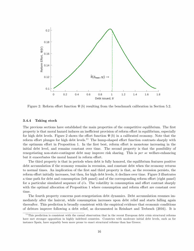
Figure 2: Reform e¤ort function (b) resulting from the benchmark calibration in Section 5.2.

3.4.4 Taking stock

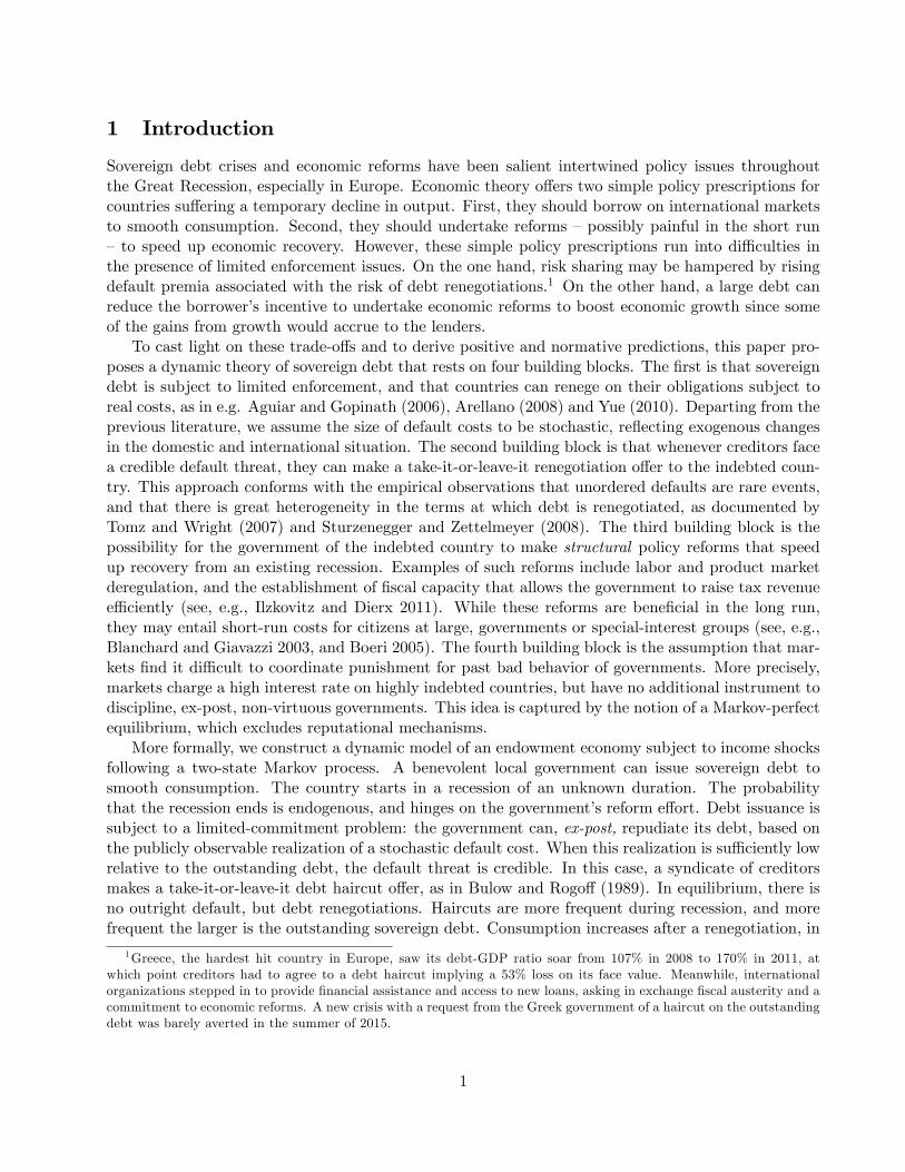
The previous sections have established the main properties of the competitive equilibrium. The �rstproperty is that moral hazard induces an ine¢ cient provision of reform e¤ort in equilibrium, especiallyfor high debt levels. Figure 2 shows the e¤ort function (b) in a calibrated economy. Note that thereform e¤ort plunges for high debt levels.11 The hump-shaped e¤ort function contrasts sharply withthe optimum e¤ort in Proposition 1. In the �rst best, reform e¤ort is monotone increasing in theinitial debt level, and remains constant over time. The second property is that the possibility ofrenegotiating non-state-contingent debt may improve risk sharing. This is per se welfare-enhancingbut it exacerbates the moral hazard in reform e¤ort.

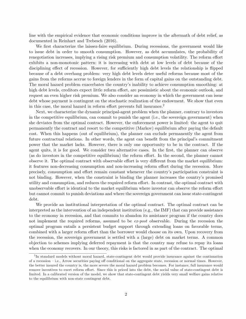
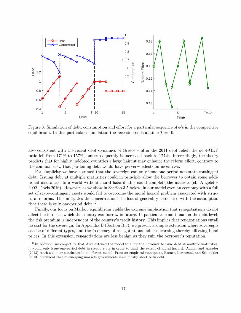
The third property is that in periods when debt is fully honored, the equilibrium features positivedebt accumulation if the economy remains in recession, and constant debt when the economy returnsto normal times. An implication of the �rst and third property is that, as the recession persists, thereform e¤ort initially increases, but then, for high debt levels, it declines over time. Figure 3 illustratesa time path for debt and consumption (left panel) and of the corresponding reform e¤ort (right panel)for a particular simulated sequence of ��s. The volatility in consumption and e¤ort contrast sharplywith the optimal allocation of Proposition 1 where consumption and reform e¤ort are constant overtime.

The fourth property concerns post-renegotiation debt dynamics. Debt accumulation resumes im-mediately after the haircut, while consumption increases upon debt relief and starts falling againthereafter. This prediction is broadly consistent with the empirical evidence that economic conditionsof debtors improve following a debt relief, as documented in Reinhart and Trebesch (2016). It is

11This prediction is consistent with the casual observation that in the recent European debt crisis structural reformshave met stronger opposition in highly indebted countries. Countries with moderate initial debt levels, such as forinstance Spain, have arguably been more prone to enact structural reforms than has Greece.

16

Time1 5 T=10 15

Deb

t

0.4

0.6

0.8

1

1.2

Con

sum

ptio

n

0.5

0.6

0.7

0.8

0.9

1

DebtConsumption

Time1 5 T=10

Ref

orm

 Effo

rt

0.13

0.14

0.15

0.16

0.17

0.18

Figure 3: Simulation of debt, consumption and e¤ort for a particular sequence of ��s in the competitiveequilibrium. In this particular siumulation the recession ends at time T = 10.

also consistent with the recent debt dynamics of Greece �after the 2011 debt relief, the debt-GDPratio fell from 171% to 157%, but subsequently it increased back to 177%. Interestingly, the theorypredicts that for highly indebted countries a large haircut may enhance the reform e¤ort, contrary tothe common view that pardoning debt would have perverse e¤ects on incentives.

For simplicity we have assumed that the sovereign can only issue one-period non-state-contingentdebt. Issuing debt at multiple maturities could in principle allow the borrower to obtain some addi-tional insurance. In a world without moral hazard, this could complete the markets (cf. Angeletos2002, Dovis 2016). However, as we show in Section 3.5 below, in our model even an economy with a fullset of state-contingent assets would fail to overcome the moral hazard problem associated with struc-tural reforms. This mitigates the concern about the loss of generality associated with the assumptionthat there is only one-period debt.12

Finally, our focus on Markov equilibrium yields the extreme implication that renegotiations do nota¤ect the terms at which the country can borrow in future. In particular, conditional on the debt level,the risk premium is independent of the country�s credit history. This implies that renegotiations entailno cost for the sovereign. In Appendix B (Section B.3), we present a simple extension where sovereignscan be of di¤erent types, and the frequency of renegotiations induces learning thereby a¤ecting bondprices. In this extension, renegotiations are less benign as they ruin the borrower�s reputation.

12 In addition, we conjecture that if we extened the model to allow the borrower to issue debt at multiple maturities,it would only issue one-period debt in steady state in order to limit the extent of moral hazard. Aguiar and Amador(2013) reach a similar conclusion in a di¤erent model. From an empirical standpoint, Broner, Lorenzoni, and Schmukler(2013) document that in emerging markets governments issue mostly short term debt.

17

3.5 Competitive equilibrium with state-contingent debt

The analysis of the competitive equilibrium was carried out thus far under the assumption that thesovereign can issue only a non-contingent asset. In this section, we extend the analysis and allow forstate-contingent debt. We continue to focus on Markov equilibria.

Let bw and b �w denote two securities paying one unit of output if the economy is in a recession or innormal times, respectively. We label these securities recession-contingent debt and recovery-contingentdebt, respectively, and denote by Qw

�b0w; b

0�w

�and Q �w

�b0w; b

0�w

�their corresponding prices. The budget

constraint in a recession is given by:

Qw�b0w; b

0�w

�� b0w +Q �w

�b0w; b

0�w

�� b0w = B (b; �; w) + c� w: (17)

Under limited commitment, the price of each security depends on the two outstanding debt levels,as both a¤ect the reform e¤ort and the probability of renegotiation.13 The sovereign�s value functioncan be written as:

V (b; �; w) = maxfb0w;b0�wg

�u�Qw�b0w; b

0�w

�� b0w +Q �w

�b0w; b

0�w

�� b0�w + w � B (b; �; w)

�(18)

�X��b0w; b

0�w

��+ �

�1�

�b0w; b

0�w

��EV

�b0w; w

�+ �

�b0w; b

0�w

�EV

�b0�w; �w

�:

Mirroring the analysis in the case of non-state-contingent debt, we proceed in two steps. First, wecharacterize the optimal reform e¤ort. This is determined by the di¤erence between the discountedutility conditional on the recession ending and continuing, respectively (cf. equation (14)):

X 0 � �b0w; b0�w�� = � �Z 1

0V�b0�w; �

0; �w�dF (�)�

Z 1

0V�b0w; �

0; w�dF (�)

�: (19)

Note that the incentive to reform would vanish under full insurance.Next, we characterize consumption and debt issuance. To this aim, consider �rst the equilibrium

asset prices. The prices of the recession- and recovery-contingent debt are given by, respectively:

Qw�b0w; b

0�w

�=

1��b0w; b

0�w

�R

�1� F

���b0w���

+1

b0w

Z �(b0w)

0

���1 (�) dF (�)

�!; (20)

Q �w

�b0w; b

0�w

�=

�b0w; b

0�w

�R

�1� F

����b0�w���

+1

b0�w

Z ��(b0�w)

0

����1 (�) dF (�)

�!: (21)

The next proposition characterizes the CEE with state-contingent debt.

Proposition 8 Assume that there exist markets for two securities delivering one unit of output if theeconomy is in recession and in normal times, respectively, and subject to the risk of renegotiation.Suppose that the economy is initially in recession. The following CEEs are satis�ed in the competitive

13Note that these assets are not Arrow-Debreu assets since their payo¤s are not conditional on the realization of �.An alternative approach would have been to follow Alvarez and Jermann (2000) and issue an Arrow-Debreu asset foreach state (w; �) and let the default-driven participation constraint serve as an endogenous borrowing constraint.

18

equilibrium:(I) If the recession continues,

u0�c0jH;w

�u0 (c)| {z }

MRS if rec. continues

= 1 +@

@b0w�b0w; b

0�w

�| {z }

>0

�R��

�b0w; b

0�w

��1� F

���b0w��� �

1��b0w; b

0�w

��| {z }>0

: (22)

(II) If the recession ends,

u0 (c0jH; �w)u0 (c)| {z }

MRS if rec. ends

= 1 +@

@b0�w�b0w; b

0�w

�| {z }

<0

�R��

�b0w; b

0�w

��1� F

��� (b0�w)

���b0w; b

0�w

�| {z };>0

(23)

where

��b0w; b

0�w

��Q �w

�b0w; b

0�w

�� b0�w

�b0w; b

0�w

� �Qw�b0w; b

0�w

�� b0w

1��b0w; b

0�w

� � 0: (24)

Moreover,

c = Qw�b0w; b

0�w

�� b0w +Q �w

�b0w; b

0�w

�� b0�w + w � B (b; �; w) ;

c0jH;w = Qw�B �w

�b0w�; B �w

�b0w���Bw

�b0w�+Q �w

�Bw�b0w�; B �w

�b0w���B �w

�b0w�+ w � b0w;

c0jH; �w = Q�B�b0w; �w

�; �w��B

�b0w; �w

�+ �w � b0�w;

where Bw�b0w�and B �w

�b0w�denote the optimal level of newly-issued recession- and recovery-contingent

debt when the recession continues, and debt is honored.

If the probability that the recession ends were exogenous, 0 = 0, consumption would be inde-pendent of the realization of the aggregate state. In this case, the CEEs imply constant consumptionc0jH;w = c0jH; �w = c where, recall, c0jH;w is consumption conditional on debt being honored in the nextperiod. However, in the general case with moral hazard, consumption falls (and recession-contingentdebt increases) whenever the economy remains in recession and debt is honored, as shown by equation(22). When the recession ends, consumption increases as shown by equation (23). Therefore, thecompetitive equilibrium features imperfect insurance, even conditional on honoring the debt.

The intuition is as follows. By issuing more recession-contingent debt, the country strengthensits incentive to make reforms, since @=@b0w > 0. This induces the sovereign to issue more recession-contingent debt than in the absence of moral hazard. This e¤ect is stronger the larger is �

�b0w; b

0�w

�which can be interpreted as the net expected gain accruing to the lenders from a marginal increasein the probability that the recession ends. On the contrary, issuing more recovery-contingent debtweakens the incentives to do reform. As a result, consumption increases if the recession ends and fallsif the recession continues (and debt is honored). This result highlights the trade-o¤ between insuranceand incentives: the country must give up insurance in order to gain credibility about its willingnessto do reforms. In addition, debt in�uences the reform e¤ort: this is increasing in the newly-issuedrecession-contingent debt and decreasing in the newly-issued recovery-contingent debt. In summary,the moral hazard problem in reform limits the possibility for the equilibrium with state-contingentdebt to smooth consumption and reform e¤ort.

19

4 Optimal contract with one-sided commitment

In the competitive equilibrium of the previous section, the sovereign cannot commit to the e¢ cientreform e¤ort and creditors cannot commit to punishments that are ex-post suboptimal. In this section,we characterize the allocation chosen by a benevolent social planner who can commit to enforcea contract even by dispensing punishments that are not ex-post optimal. However, the borrowercontinues to be subject to limited commitment. This limits the planner�s ability to punish deviationsfrom the optimal contract. In particular, the maximum punishment the planner can impose is toterminate the contract and let the sovereign resort to the competitive equilibrium. In the next section,we interpret this allocation as the result of an assistance program managed by an international agency(e.g., the IMF) that can commit to terminate its program in case of non-compliance. We consider twoscenarios. In the �rst, the reform e¤ort is observable, while in the second it is not. We continue toassume, as in the competitive equilibrium, that the realization of � is publicly observable.

The problem is formulated as a one-sided commitment program, following Ljungqvist and Sargent(2012) and based on a promised-utility approach in the vein of Spear and Srivastava (1987), Thomasand Worrall (1988 and 1990) and Kocherlakota (1996).

We denote by � the utility promised to the risk-averse agent in the beginning of the period, beforethe realization of �. � is the key state variable of the problem. We denote by �!� and !� the promisedcontinuation utilities conditional on the realization � and on the aggregate state �w and w, respectively.P (�) and �P (�) denote the expected present value of pro�ts accruing to the principal conditional ondelivering the promised utility � in the most cost-e¤ective way in recession and in normal times,respectively. The planning problem is evaluated after the uncertainty about the aggregate state hasbeen resolved (i.e., the economy is either in recession or in normal times in the current period), butbefore the realization of � is known. In Appendix B (Proposition 16), we prove, following the strategyin Thomas and Worrall (1990), that the functional equations de�ned in equations (25) and (30) beloware contraction mappings, that the pro�t functions P (�) and �P (�) are decreasing, strictly concaveand continuously di¤erentiable, and that the associated maximands are unique.

4.1 Normal times

In normal times, the optimal value �P (�) satis�es the following functional equation:

�P (�) = maxfc�;�!�g�2@

Z@

��w � �c� +

1

R�P (�!�)

�dF (�) ; (25)

where the maximization is subject to the constraintsZ@[u (�c�) + ��!�] dF (�) � �; (26)

u (�c�) + ��!� � W (0; �w)� �; � 2 @; (27)

�c� 2 [0; �w]; �; �!� 2 [W (0; �w)� E [�] ;W (0; �w)]:

The inequality (26) is a promise-keeping constraint, whereas (27) is a participation constraint (PC).Note that the outside option for the agent is equivalent to the value of default in the competitiveequilibrium.

The application of recursive methods allows us to establish the following proposition.

20

Proposition 9 Assume the economy is in normal times. (I) For all realizations � such that the PCof the agent, (27), is binding, �!� > � and the solution for (�c�; �!�) is determined by the followingconditions:

u0 (�c�) = �1

�P 0 (�!�); (28)

u (�c�) + ��!� =W (0; �w)� �: (29)

The solution is not history-dependent, i.e., the initial promise, �; does not matter. (II) For all real-izations � such that the PC of the agent, (27), is not binding, �!� = � and �c� = �c (�), where �c (�) isdetermined by (28). The solution is history-dependent.

The optimal contract has standard properties. Whenever the agent�s PC is not binding, consump-tion and promised utility remain constant over time. Whenever the PC binds, the planner increasesthe agent�s consumption and promised utility in order to meet her PC.

4.2 Recession

When the economy is in recession, the contract speci�es also an e¤ort level. We consider �rst the casein which the reform e¤ort is observable. In this case, the planner terminates the contract wheneverthe agent deviates from the e¢ cient e¤ort level. We assume that when the agent deviates at time t,she is settled with the default cost at t+ 1. Note that this allocation is equivalent to a decentralizedequilibrium in which the sovereign can issue debt contingent both on the aggregate level and on theborrower�s e¤ort.

The reform e¤ort associated with a deviation is given by

pdev = arg maxp2[p;�p]

�X (p) + � ((1� p)W (0; w) + pW (0; �w))

! X 0 (pdev) = � (W (0; �w)�W (0; w))

Then, the continuation utility from a deviation is given by

�dev � �X (pdev) + ��(1� pdev)W (0; w) + pdevW (0; �w)� E

��0��;

where E��0�denotes the expected value of �0:

We can now characterize the optimal contract under recession

P (�) = maxfc�;p�;�!�;!�g�2@

Z@

�w � c� +

1

R

�(1� p�)P

�!��+ p� �P (�!�)

��dF (�) ; (30)

where the maximization is subject to the constraintsZ@

�u�c���X (p�) + �

�(1� p�)!� + p��!�

��dF (�) � �; (31)

u�c���X (p�) + �

�(1� p�)!� + p��!�

�� W (0; w)� �; � 2 @; (32)

�X (p�) + ��(1� p�)!� + p��!�

�� �dev (33)

c� 2 [0; �w]; p� 2 [p; �p]; �; !� 2 [W (0; w)� E [�] ;W (0; �w)]; �!� 2 [W (0; �w)� E [�] ;W (0; �w)]:

21

We prove in Appendix B (Proposition 16) that the program is concave, and that the FOCs arenecessary and su¢ cient. The FOCs with respect to �!�; !�; and p� (see equations (63)�(66) inAppendix A) yield:14

�P 0 (�!�) = P 0�!��

(34)

X 0 (p�) = ���!� � !�

�� R�1

P 0�!�� � �P (�!�)� P �!��� : (35)

Equation (34) establishes that the planner equates the marginal pro�t loss associated with promisedutilities in the two aggregate states. (35) establishes that e¤ort is set at the constrained e¢ cient level.The two terms on the right hand-side are the bene�ts accruing to the agent and to the principal,respectively. Note that in the competitive equilibrium the sovereign only takes into consideration theprivate gain of exerting e¤ort, so the second term is missing.

The IC constraint may or may not be binding. When it is binding, (34), (35) and the IC constraintpin down a unique (constant) level of promised utilities and e¤ort. We state this formally in thefollowing Lemma.

Lemma 5 When the IC is binding, e¤ort and promised utilities are constant at the levels �!� = �!�;!� = !

� and p� = p�, where the triplet (p�; !�; �!�) is uniquely determined by the IC constraint (33)holding with equality, (34), and (35).

When the IC constraint is not binding, consumption is pinned down by the following standardFOC (see equations (63) and (64) in Appendix A):

u0�c��= � 1

P 0�!�� : (36)

This condition does not hold when the IC constraint is binding, since the planner must in this casedistort the consumption margin.

We characterize the optimal contract by distinguishing two cases. Proposition 10 covers the casein which the initial promise utility is high and the IC constraint is not binding irrespective of therealization of �. Proposition 11 covers the case in which the initial promise utility is low and the ICconstraint is binding for a non-empty range of realizations of �.

It is useful to de�ne ~�(�) as the threshold realization of � such that the participation constraintis binding. In particular, ~�(�) is implicitly de�ned by the promise-keeping constraint (31),

� =W (0; w)�"Z ~�(v)

0�dF (�) + ~�(�)

h1� F (~�(v))

i#; (37)

where ~�(�) is decreasing in �.

Proposition 10 Suppose that the economy starts in a recession with promised utility � � !�: Then,the IC constraint (33) is never binding (irrespective of �), and the optimal contract is characterizedas follows:14To see why the solution to (34)�(35) is unique, note that the concavity and monotonicity of P and �P imply that

Equation (34) determines a positive relationship between !� and �!�. Thus, Equation (35) yields an implicit decreasingrelationship between p� and !� and an implicit increasing relationship between p� and �!�.

22

1. If � < ~�(�), the PC is binding, and the solution for�c�; p�; !�; �!�

�is determined by (34), (35),

(36) and by (32) holding with equality. Moreover, !� > �.

2. If � � ~�(�), the PC is slack, and the solution for�c�; p�; !�; �!�

�is given by !� = �; c� = c (�) ;

�!� = �! (�) ; and p� = p (�), where the functions c (�) ; �! (�) and p (�) are determined by (36),(34), (35), respectively. The solution is history-dependent. The reform e¤ort is decreasing andconsumption and future promised utility are increasing in �.

When � < !�, the solution of Proposition 10 would violate the IC constraint in some states. Thus,the planner must either reduce the demands on e¤ort or increase the promise utilities so that the ICconstraint holds. The following proposition characterizes the optimal contract in this case.

Proposition 11 Suppose that the economy starts in a recession with promised utility � < !�. Then,the IC constraint (33) is binding in some states, and the optimal contract is characterized as follows:

1. If � < ~�(!�), the PC is binding while the IC is not binding. The solution is not history-dependentand is determined as in Proposition 10, part 1 (in particular, !� > !

� and p� < p�).

2. If � 2 [~�(!�); ~�(�)], both the PC and the IC are binding. E¤ort and promised utilities are equalto (p�; !�; �!�) as given by Lemma 5. Consumption is determined by (32) and (33) jointly, whichyield:

c�� = u�1 (W (0; w)� �� �dev) : (38)

Consumption and e¤ort are lower and promised utilities are higher than in the absence of an ICconstraint.

3. If � > ~�(�), the IC is binding, while the PC is not binding. E¤ort and promised utilities areequal to (p�; !�; �!�) : Consumption is constant across � and is determined by (31) and (33),which yield:

c�� = u�1�W (0; w)� ~�(�)� �dev

�: (39)

Consumption and e¤ort are lower and promised utilities are higher than in the absence of an ICconstraint.

Consider an economy where, initially, � < !�. If � < ~�(!�) (case 1), the binding PC inducesthe planner to set an e¤ort level so low that the IC is not binding. The allocation is not history-dependent, and the characterization of Proposition 10 applies. For all levels of � larger than ~�(!�),the IC is binding, and Lemma 5 implies that e¤ort and promised utility are equal to (p�; !�; �!�), i.e. themaximum e¤ort and the minimum promised future utilities consistent with the IC. In particular, if � 2[~�(!�); ~�(�)] (case 2), consumption is pinned down jointly by the PC and IC. In this case, consumptionis decreasing in �. Finally, if � > ~�(�) (case 3) the PC is slack, and consumption is constant across �and determined by the promise-keeping constraint. Note that whenever the IC constraint is binding(cases 2 and 3), both consumption and e¤ort are lower than in Proposition 10. Intuitively, the plannersatis�es the IC and promise-keeping contraints by reducing current consumption and e¤ort, and byincreasing promised utilities relative to the case in which the IC constraint is not binding. Thus, thecontract provides less consumption insurance but more e¤ort smoothing.

Note that the IC constraint binds for at most one period. After that either the recession ends, orthe planner sets the promised utility to the level !�: Either way, the IC constraint becomes irrelevant,and the equilibrium is characterized as in Proposition 10.

23

Time1 5 T=10 15

Con

sum

ptio

n

0.64

0.66

0.68

0.7

0.72

0.74

0.76

0.78

Ref

orm

 Effo

rt

0.13

0.14

0.15

0.16

0.17

0.18

0.19

0.2

0.21

ConsumptionReform Effort

Time1 5 T=10 15

Pro

mis

ed­U

tility

, Rec

essi

on

­22.15

­22.05

­21.95

­21.85

­21.75

­21.65

Pro

mis

ed­U

tility

, Nor

mal

 Tim

es

­1.85

­1.845

­1.84

­1.835

­1.83

RecessionNormal Times

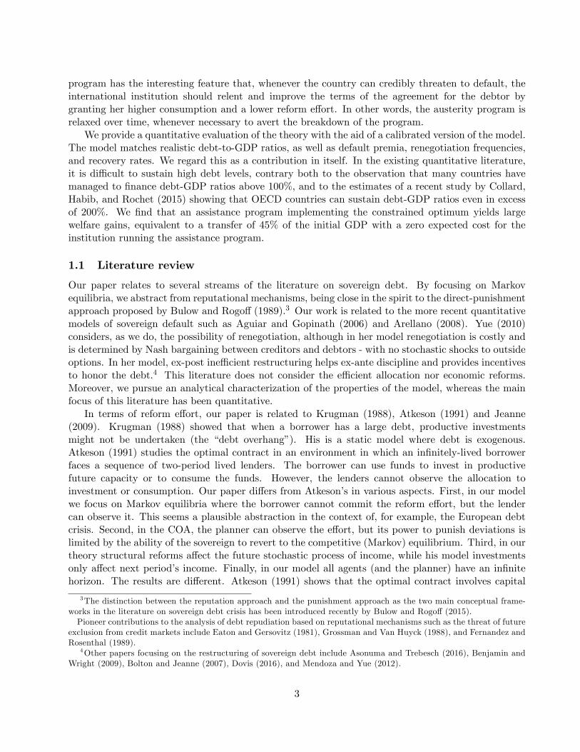
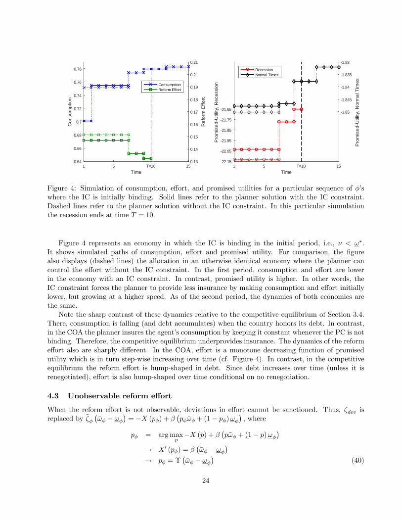
Figure 4: Simulation of consumption, e¤ort, and promised utilities for a particular sequence of ��swhere the IC is initially binding. Solid lines refer to the planner solution with the IC constraint.Dashed lines refer to the planner solution without the IC constraint. In this particular siumulationthe recession ends at time T = 10.

Figure 4 represents an economy in which the IC is binding in the initial period, i.e., � < !�.It shows simulated paths of consumption, e¤ort and promised utility. For comparison, the �gurealso displays (dashed lines) the allocation in an otherwise identical economy where the planner cancontrol the e¤ort without the IC constraint. In the �rst period, consumption and e¤ort are lowerin the economy with an IC constraint. In contrast, promised utility is higher. In other words, theIC constraint forces the planner to provide less insurance by making consumption and e¤ort initiallylower, but growing at a higher speed. As of the second period, the dynamics of both economies arethe same.

Note the sharp contrast of these dynamics relative to the competitive equilibrium of Section 3.4.There, consumption is falling (and debt accumulates) when the country honors its debt. In contrast,in the COA the planner insures the agent�s consumption by keeping it constant whenever the PC is notbinding. Therefore, the competitive equilibrium underprovides insurance. The dynamics of the reforme¤ort also are sharply di¤erent. In the COA, e¤ort is a monotone decreasing function of promisedutility which is in turn step-wise increasing over time (cf. Figure 4). In contrast, in the competitiveequilibrium the reform e¤ort is hump-shaped in debt. Since debt increases over time (unless it isrenegotiated), e¤ort is also hump-shaped over time conditional on no renegotiation.

4.3 Unobservable reform e¤ort

When the reform e¤ort is not observable, deviations in e¤ort cannot be sanctioned. Thus, �dev isreplaced by ~��

��!� � !�

�= �X (p�) + �

�p��!� + (1� p�)!�

�; where

p� = argmaxp�X (p) + �

�p�!� + (1� p)!�

�! X 0 (p�) = �

��!� � !�

�! p� = �

��!� � !�

�(40)

24

Moreover, the IC constraint always holds. Note that e¤ort is now ine¢ ciently provided, since theagent does not internalize the bene�t of e¤ort provision that accrues to the planner.

The FOCs with respect to !� and �!�, together with the envelope condition, yield (see proof ofProposition 12 in Appendix A):

P 0�!��� �P 0 (�!�) =

��0(�!� � !�)�(�!� � !�)

+�0(�!� � !�)1��(�!� � !�)

���P (�!�)� P

�!���

(41)

1

u0(c�)= �

�P 0�!���

�0(�!� � !�)1��(�!� � !�)

��P (�!�)� P

�!����

: (42)

The FOC (41) is the analogue of (34). Note that the planner does no longer equalize the marginalcost of promised utility in the two states. The reason is that increasing the di¤erence in promisedutility is the only way for the planner to increase e¤ort provision. Thus, the unobservability of e¤ortreduces insurance.

We can now establish the following proposition.

Proposition 12 Suppose that the economy starts in a recession and e¤ort is not observable. Then,the optimal contract is characterized as follows: (i) p� = �

��!� � !�

�as in (40), and (ii):

1. If � < ~�(�); the PC is binding, and the solution for�c�; !�; �!�

�is determined by (41), (42),

and by (32) holding with equality.

2. If � � ~�(�); the PC is slack, and the solution for�c�; !�; �!�

�is determined by (41), (42), and

by the FOC for consumption

u0�c��= � 1

P 0 (�):

The solution is history-dependent (i.e., c� = c (�) ; !� = ! (�) < �; and �!� = �! (�)). As long asthe recession persists and the PC remains slack, consumption and promised utilities are fallingand e¤ort is increasing over time.

The results when e¤ort is not unobservable di¤er sharply from the case in which e¤ort is observ-able and the planner has commitment. In this case, the dynamics are more similar to those of thecompetitive equilibrium without commitment. Consumption falls over time whenever � is su¢ cientlyhigh. This is the way the planner gives dynamic incentives: she curtails insurance in order to extracthigher e¤ort over time.

4.4 Comparison between the COA and the competitive equilibrium

The �rst result is that in normal times the planner allocation in Proposition 9 is identical to thecompetitive equilibrium. To establish the equivalence result we return, �rst, to the competitive equi-librium. Let

�� (b) =�1� F

��� (b)

��b+

Z ��(b)

0b̂ (�; �w) dF (�) (43)

25

denote the expected value for the creditors of an outstanding debt b before the current-period un-certainty is resolved. Note that �� (b) yields the expected debt repayment, which is lower than theface value of debt, since in some states of nature debt is renegotiated. To prove the equivalence, wepostulate that �� (b) = �P (�) ; and show that in this case � = EV (b; �w).15 If the planning allocationwere more e¢ cient than the equilibrium, and we would �nd that � > EV (b; �w) :

Proposition 13 Assume that the economy is in normal times. The competitive equilibrium is equiv-alent to the COA in Proposition 9, namely, �� (b) = �P (�), � = EV (b; �w) :

Intuitively, renegotiation provides the market economy with su¢ ciently many state contingenciesto attain second-best e¢ ciency. This result hinges on two features of the renegotiation protocol. First,renegotiation averts any real loss associated with unordered default. Second, creditors have all thebargaining power in the renegotiation game.16 Moreover, note that in normal times there is no issueof commitment since e¤ort is only exerted in recession.

The equivalence result of Proposition 13 hinges on the assumption that normal times is an absorbingstate that will be relaxed in Section 5 below. Moreover, even in the current environment, it does notcarry over to recessions. We will show that in recession the result hinges on two critical assumptionsabout the planning problem: whether e¤ort is observable and whether the sovereign can issue state-contingent debt.

It is instructive to start by analyzing with a case in which there is no moral hazard problem, i.e.,the probability that the recession ends is independent of the reform e¤ort (i.e., = p).

Proposition 14 If the probability that the recession ends is independent of the reform e¤ort (i.e., = p), then the competitive equilibrium with state-contingent debt is constrained e¢ cient conditionalon p. In particular, if p = p (EV (b; w)) ; i.e., e¤ort is set at the constrained optimum level, then thecompetitive equilibrium with state-contingent debt is a COA, namely, �(b) = P (�), � = EV (b; w),where �(b) is the valuation of debt conditional on staying in recession before the realization of �:

The equivalence of Proposition 14 breaks down if there is moral hazard, and the market cannotcommit to punish deviations in reform e¤ort. The qualitative dynamics are also di¤erent. In thecompetitive equilibrium with state-contingent debt of Section 3.5, consumption falls (and recession-contingent debt increases) whenever the economy remains in recession and debt is honored, as shownby equation (22). On the contrary, consumption increases whenever the recession ends, as shown byequation (23).

Interestingly, the competitive equilibrium with state-contingent debt can sustain a planning allo-cation where the planner cannot observe e¤ort. The result is especially interesting as e¤ort can inprinciple be observed in the competitive equilibrium. However, this is not useful because of the lackof commitment. The proof of this equivalence is harder, as it is di¢ cult to prove that the planningproblem is concave in general when e¤ort is not observable. This is a common problem in the liter-ature (see Renner and Schmedders 2015). Therefore, the equivalence is stated under the assumptionthat the �rst-order conditions are su¢ cient for the planning problem. This assumption can be veri�ednumerically, as we do in the numerical analysis below.15Recall that EV (b; �w) =

R@ V (b; �; �w) dF (�) denotes the discounted utility accruing to a country with the debt level

b in the competitive Markov equilibrium.16We view this as a useful benchmark. In reality, renegotiations may entail costs associated with legal proceeds and

lawsuits, trade retaliation, temporary market exclusion, etc. Also, creditors may not have the full ex-post bargainingpower at the renegotiation stage as in Yue (2010). This would reduce the amount of loans creditors can recover. In allthese cases, the competitive equilibrium would fail to implement the COA.

26

Proposition 15 Assume that the economy is in recession. Consider the planning allocation withunobservable e¤ort of Proposition 12 where the outside option W (0; w) in equation (32) is the valuefunction associated with a competitive equilibrium with state-contingent debt. Assume that the �rst-order conditions are necessary and su¢ cient. This planning allocation can be sustained as a competitiveequilibrium with state contingent debt (cf. Proposition 3.5), namely, �(b) = P (�), � = EV (b; w).

The proposition establishes that if e¤ort is not observable, then, commitment is of no value tothe planner. Then, the market can decentralized the planner allocation in the vein of Prescott andTownsend (1984). An immediate corollary of Proposition 15 is that the planning allocation of Propo-sition 12 is more e¢ cient than the equilibrium with non-state-contingent debt.

It is also useful to comment on the relationship between the competitive equilibrium and theplanning allocation with observable e¤ort of Proposition 10. In order to decentralize the optimalcontract as a competitive equilibrium with state-contingent debt, the sovereign should be able tocommit to the e¢ cient reform level. In particular, one could consider a market for state-contingentdebt where payments are also conditioned on the exerted e¤ort level. At the optimal e¤ort level, thesovereign would promise a repayment that is equivalent to the optimal contract. For any other e¤ortlevel, the payment would be that associated with the maximum debt level �b. This implies that if thereis a deviation from the equilibrium e¤ort debt would be renegotiated with certainty in the followingperiod. This ensures that the IC constraint holds in the competitive equilibrium. In other words, thistype of state-contingent debt is a stand-in for commitment.

4.5 Interpreting the COA as an austerity program

In this section, we discuss a policy-relevant institutional interpretation of the COA. Consider a stand-by program run by an international institution, e.g., the IMF. Like the planner, and unlike the market,the IMF can punish deviations, but cannot get around the limited commitment problem, i.e., theindebted country can pay the default cost and walk away unilaterally. We show that the plannerallocation can be interpreted as a combination of transfers (or loans), repayment schedules, reformprogram and renegotiation strategy. This program has two key features. First, the country cannotrun an independent �scal policy, i.e., it is not allowed to issue additional debt in the market. Second,the program is subject to renegotiation. More precisely, whenever the country credibly threatens toabandon the program, the international institution should sweeten the deal by increasing the transfers,reducing the required e¤ort, and reducing the debt the country owes when the recession ends. Whenno credible threat of default is on the table, consumption and reform e¤ort should be held constant aslong as the recession lasts. When the recession ends, the international institution receives a paymentfrom the country, �nanced by issuing debt in the market.

Let � denote the present discounted utility guaranteed to the country when the program is �rstagreed upon. Let c� (�) and p� (�) be the consumption and reform e¤ort associated with the promisedutility in the planning problem. Upon entering the program, the country receives a transfer equal toT (�) + b0; where T (�) = c� (�) � w (note that T (�) could be negative). In the subsequent periods,the country is guaranteed the transfer �ow T (�) so long as the recession lasts and there is no crediblerequest of renegotiating the terms of the austerity program. In other words, the international insti-tution �rst bails out the country from its obligations to creditors, and then becomes the sole residualclaimant of the country�s sovereign debt. The country is also asked to exert a reform e¤ort p� (�). Ifthe country faces a low realization of � and threatens to leave the program, the institution improvesthe terms of the program so as to match the country�s outside option. Thereafter, consumption and

27

e¤ort are held constant at new higher and lower levels, respectively, as in the planner�s allocation.And so on, for as long as the recession continues.

As soon as the recession ends, the country owes a debt bN to the international institution, deter-mined by the equation

Q (bN ; �w)� bN = c� (�N )� �w + bN :

Here �N is the expected utility granted to the country after the most recent round of renegotiation.After receiving this payment, the international institution terminates the program and lets the country�nance its debt in the market.

This program resembles an austerity program, in the sense that the country is prevented fromrunning an independent �scal policy and reform program. In particular, the country would like toissue extra debt after entering the stand-by agreement, so austerity is a binding constraint. In addition,the country would like to shirk on the reform e¤ort prescribed by the agreement. Thus, the sovereignwould like to (temporarily) deviate from the optimal plan, and promises about future transfers is anessential feature of the program.

A distinctive feature of the assistance program is that the international institution sets "harsh"entry conditions in anticipation of future renegotiations. How harsh these conditions are depends on�: In turn, � may re�ect a political decision about how many (if any) own resources the internationalinstitution wishes to commit to rescuing the indebted country. A natural benchmark is to set � suchthat the international institution makes zero pro�ts (and zero losses) in expectation. Whether, ex-post, the international institution makes net gains or losses hinges on the duration of the recessionand on the realized sequence of ��s.

Another important policy implication of our analysis is that it would be subptimal for the interna-tional institution to commit never to accept any renegotiation. On the contrary, such a policy wouldlead to welfare losses because, on the one hand, there would be ine¢ cient default in equilibrium; on theother hand, the country could not expect future improvements, and therefore would not accept a verylow initial consumption, or a very high reform e¤ort. If the international institution�s expected pro�twere zero in both programs, the country would receive a lower expected utility from the alternative(no renegotiation) program.

In summary, our theory prescribes a pragmatic approach to debt renegotiation. Credible threats ofdefault should be appeased by reducing the debt and softening the austerity program. Such approachis often criticized for creating bad incentives. In our model, such appeasement is precisely the optimalpolicy under the reasonable assumption that penalties on sovereign countries for breaking an agreementare limited.

5 Recurrent recessions and quantitative analysis

In this section, we generalize the model and study its quantitative properties from a positive andnormative standpoint.

5.1 Recurrent recessions

In order to align the model with the data, we relax the assumption that there exists an absorbing stateand assume, instead, that in normal times the economy falls into a deep recession with an exogenousprobability p̂. Additionally, we relax the assumption that �R = 1: In particular, we emphasize the casein which �R < 1 since this ensures that the competitive equilibrium has a non-degenerate stationarydistribution (cf. Aiyagari 1994).

28

While most properties discussed in the previous section carry over to this generalization, theeconomy will feature some qualitative di¤erences relative to the analysis in Sections 3-4 above. First,in normal times, the sovereign engages in precautionary savings to accumulate a bu¤er in expectation offuture recessions. Therefore, consumption and wealth are not constant during normal times even whendebt is honored.17 The qualitative debt dynamics in the stationary equilibrium have the followingfeatures. In normal times, debt (when honored) tends to a target level. During recession, whenhonored, debt increases unambiguously with dynamics qualitatively similar to those of Section 3.4.

Assuming �R < 1 also a¤ects the planning allocation. The �rst-best now features ever-decreasingconsumption and increasing e¤ort when the economy is in recession. The planning allocation withone-sided commitment and observable e¤ort of Section 4.2 is a¤ected in a similar fashion: when neitherthe participation nor the IC constraint are binding, the allocation yields rising e¤ort and decliningconsumption and promised utility. Consequently, the IC constraint may bind recurrently: the ICconstraint sets a �oor to the continuation utility below which the agent would choose to exit thecontract and resort to market �nancing.

5.2 Calibration

We calibrate the model economy to match salient moments of observed debt-to-GDP ratios and defaultpremia for Greece, Ireland, Italy, Portugal, and Spain (GIIPS). A model period corresponds to oneyear. We set p̂ = 0:01. This low probability is intended to capture rare and severe downturns ignoringstandard �uctuations on a business cycle frequency. We normalize the GDP during normal times to�w = 1 and assume that the recession causes a drop in income of 40%, i.e., w = 0:6� �w. This correspondsto the fall of GDP per capita for Greece between 2007 and 2013, relative to trend.18 Since we focuson the return on government debt, the annual real gross interest rate is set to R = 1:02. The utilityfunction is assumed to be CRRA with a relative risk aversion of 2.

We calibrate the discount factor � to target a stationary average debt 54.9% of GDP in line withthe evidence for the GIIPS over the period 1950-2015.19 We assume an isoelastic e¤ort cost function,X(p) = �

1+1='(p)1+1=', where � regulates the average level of e¤ort and ' regulates the elasticity of

reform e¤ort to changes in the return to reforms. We calibrate the two parameters, ' and �; so asto match two points on the equilibrium e¤ort function (b). In particular, we target the e¤ort atthe debt limit,

��b�= 10%, so that a country at the debt limit would choose an e¤ort inducing an

expected duration of the recession of one decade (we have Greece in mind). Moreover, we target amaximum e¤ort, maxb(b) = 20%, inducing an expected recession duration of �ve years (we haveIceland and Ireland in mind).

Finally, we calibrate the support and the distribution of the default cost � so that the modelmatches key moments of the quantity and price of sovereign debt. One common problem in thequantitative literature on sovereign debt is that those models fail to match observed values of debt-to-GDP ratios under standard parameterization (Arellano 2008; Yue 2010). This is not a problemin our model. In fact, the maximum default cost realization �� is calibrated to target a debt limitduring normal times of �b= �w = 178% which corresponds to the maximum sustainable debt reported

17Moreover, as anticipated above, Proposition 13 is no longer true.18GDP per capita of Greece fell from 22�700 to 16�800 Euro between 2007 and 2013 (Eurostat, nama_10_pc series).

The annualized growth rate between 1997 and 2007 was 3.6%. The fall in output between 2007 and 2013 relative totrend was therefore 40%.19We use the debt-to-GDP ratios reported by Eurostat for the period 1995-2015. For earlier periods, we chain the

debt levels back to 1950 with the series reported in the Reinhart and Rogo¤ (2010) dataset.

29

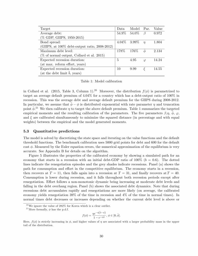
Target Data Model Par. ValueAverage debt: 54.9% 54.0% � 0.972(% GDP, GIIPS, 1950-2015)Bond spread: 4.04% 3.99% � 1.804(GIIPS, at 100% debt-output ratio, 2008-2012)Maximum debt level: 178% 176% �� 2.134(% of normal output, Collard et al. 2015)Expected recession duration: 5 4.95 ' 14.24(at max. reform e¤ort, years)Expected recession duration: 10 9.99 � 14.55(at the debt limit �b, years)

Table 1: Model calibration

in Collard et al. (2015, Table 3, Column 1).20 Moreover, the distribution f(�) is parametrized totarget an average default premium of 4:04% for a country which has a debt-output ratio of 100% inrecession. This was the average debt and average default premium for the GIIPS during 2008-2012.In particular, we assume that ��� � is distributed exponential with rate parameter � and truncationpoint ��.21 We then calibrate � to target the above default premium. Table 1 summarizes the targetedempirical moments and the resulting calibration of the parameters. The �ve parameters �,�, ��, ',and � are calibrated simultaneously to minimize the squared distance (in percentage and with equalweights) between the empirical and the model generated moments.

5.3 Quantitative predictions

The model is solved by discretizing the state space and iterating on the value functions and the defaultthreshold functions. The benchmark calibration uses 5000 grid points for debt and 600 for the defaultcost �: Measured by the Euler equation errors, the numerical approximation of the equilibrium is veryaccurate. See Appendix B for details on the algorithm.

Figure 5 illustrates the properties of the calibrated economy by showing a simulated path for aneconomy that starts in a recession with an initial debt-GDP ratio of 100% (b = 0:6). The dottedlines indicate the renegotiation episodes and the grey shades indicate recessions. Panel (a) shows thepath for consumption and e¤ort in the competitive equilibrium. The economy starts in a recession,then recovers at T = 11, then falls again into a recession at T = 31, and �nally recovers atT = 40.Consumption is lower during recession, and it falls throughout both recession periods except afterrenegotiation. E¤ort follows a non-monotonic dynamic being increasing at moderate debt levels andfalling in the debt overhang region. Panel (b) shows the associated debt dynamics. Note that duringrecessions debt accumulates rapidly and renegotiations are more likely (on average, the calibratedeconomy yields renegotiation 39% of the time in recession and 4% of the time in normal times). Innormal times debt decreases or increases depending on whether the current debt level is above or

20We ignore the value of 282% for Korea which is a clear outlier.21More formally, � has the p.d.f.

f(�) =�e��(

����)

1� e����, � 2 [0; ��]:

Here, f(�) is strictly increasing in �; and higher values of � are associated with a larger probability mass in the uppertail of the distribution.

30

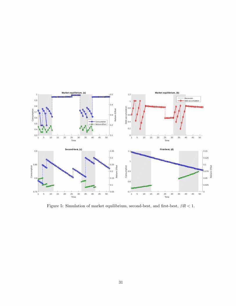
Time1 5 10 15 20 25 30 35 40 45 50

Con

sum

ptio

n

0.3

0.4

0.5

0.6

0.7

0.8

0.9

1Market equilibrium, (a)

Ref

orm

 Effo

rt

0.1

0.2

0.3

0.4

0.5

ConsumptionReform Effort

Time1 5 10 15 20 25 30 35 40 45 50

Deb

t acc

umul

atio

n

0

0.2

0.4

0.6

0.8

1

1.2Market equilibrium, (b)

RecessionDebt accumulation

Time1 5 10 15 20 25 30 35 40 45 50

Con

sum

ptio

n

0.75

0.8

0.85

0.9Second­best, (c)

Ref

orm

 Effo

rt

0.05

0.1

0.15

0.2

0.25

0.3

0.35

Time1 5 10 15 20 25 30 35 40 45 50

Con

sum

ptio

n

0.7

0.8

0.9

1

1.1First­best, (d)

Ref

orm

 Effo

rt

0

0.025

0.05

0.075

0.1

0.125

0.15

Figure 5: Simulation of market equilibrium, second-best, and �rst-best, �R < 1:

31

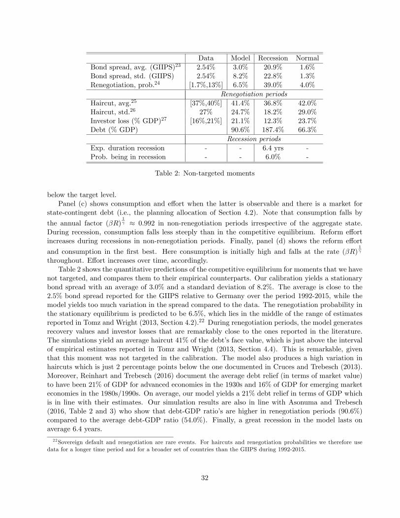
Data Model Recession NormalBond spread, avg. (GIIPS)23 2.54% 3.0% 20.9% 1.6%Bond spread, std. (GIIPS) 2.54% 8.2% 22.8% 1.3%Renegotiation, prob.24 [1.7%,13%] 6.5% 39.0% 4.0%

Renegotiation periodsHaircut, avg.25 [37%,40%] 41.4% 36.8% 42.0%Haircut, std.26 27% 24.7% 18.2% 29.0%Investor loss (% GDP)27 [16%,21%] 21.1% 12.3% 23.7%Debt (% GDP) 90.6% 187.4% 66.3%

Recession periodsExp. duration recession - - 6.4 yrs -Prob. being in recession - - 6.0% -

Table 2: Non-targeted moments

below the target level.Panel (c) shows consumption and e¤ort when the latter is observable and there is a market for

state-contingent debt (i.e., the planning allocation of Section 4.2). Note that consumption falls by

the annual factor (�R)1 � 0:992 in non-renegotiation periods irrespective of the aggregate state.

During recession, consumption falls less steeply than in the competitive equilibrium. Reform e¤ortincreases during recessions in non-renegotiation periods. Finally, panel (d) shows the reform e¤ort

and consumption in the �rst best. Here consumption is initially high and falls at the rate (�R)1

throughout. E¤ort increases over time, accordingly.Table 2 shows the quantitative predictions of the competitive equilibrium for moments that we have

not targeted, and compares them to their empirical counterparts. Our calibration yields a stationarybond spread with an average of 3.0% and a standard deviation of 8.2%. The average is close to the2.5% bond spread reported for the GIIPS relative to Germany over the period 1992-2015, while themodel yields too much variation in the spread compared to the data. The renegotiation probability inthe stationary equilibrium is predicted to be 6.5%, which lies in the middle of the range of estimatesreported in Tomz and Wright (2013, Section 4.2).22 During renegotiation periods, the model generatesrecovery values and investor losses that are remarkably close to the ones reported in the literature.The simulations yield an average haircut 41% of the debt�s face value, which is just above the intervalof empirical estimates reported in Tomz and Wright (2013, Section 4.4). This is remarkable, giventhat this moment was not targeted in the calibration. The model also produces a high variation inhaircuts which is just 2 percentage points below the one documented in Cruces and Trebesch (2013).Moreover, Reinhart and Trebesch (2016) document the average debt relief (in terms of market value)to have been 21% of GDP for advanced economies in the 1930s and 16% of GDP for emerging marketeconomies in the 1980s/1990s. On average, our model yields a 21% debt relief in terms of GDP whichis in line with their estimates. Our simulation results are also in line with Asonuma and Trebesch(2016, Table 2 and 3) who show that debt-GDP ratio�s are higher in renegotiation periods (90.6%)compared to the average debt-GDP ratio (54.0%). Finally, a great recession in the model lasts onaverage 6.4 years.

22Sovereign default and renegotiation are rare events. For haircuts and renegotiation probabilities we therefore usedata for a longer time period and for a broader set of countries than the GIIPS during 1992-2015.

32

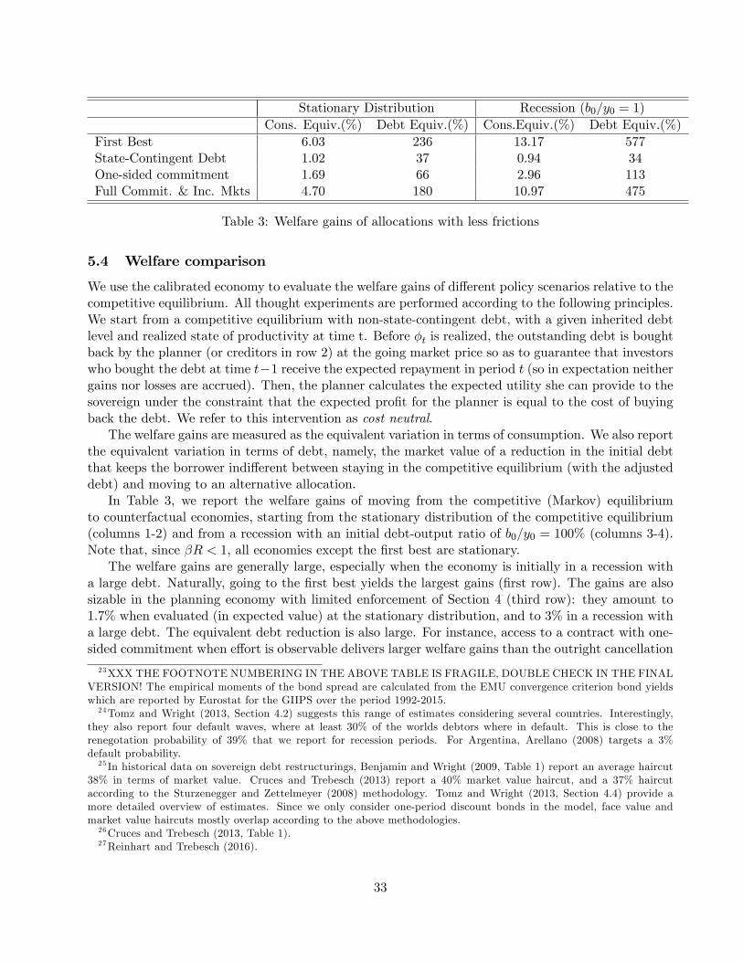
Stationary Distribution Recession (b0=y0 = 1)Cons. Equiv.(%) Debt Equiv.(%) Cons.Equiv.(%) Debt Equiv.(%)

First Best 6.03 236 13.17 577State-Contingent Debt 1.02 37 0.94 34One-sided commitment 1.69 66 2.96 113Full Commit. & Inc. Mkts 4.70 180 10.97 475

Table 3: Welfare gains of allocations with less frictions

5.4 Welfare comparison

We use the calibrated economy to evaluate the welfare gains of di¤erent policy scenarios relative to thecompetitive equilibrium. All thought experiments are performed according to the following principles.We start from a competitive equilibrium with non-state-contingent debt, with a given inherited debtlevel and realized state of productivity at time t. Before �t is realized, the outstanding debt is boughtback by the planner (or creditors in row 2) at the going market price so as to guarantee that investorswho bought the debt at time t�1 receive the expected repayment in period t (so in expectation neithergains nor losses are accrued). Then, the planner calculates the expected utility she can provide to thesovereign under the constraint that the expected pro�t for the planner is equal to the cost of buyingback the debt. We refer to this intervention as cost neutral.

The welfare gains are measured as the equivalent variation in terms of consumption. We also reportthe equivalent variation in terms of debt, namely, the market value of a reduction in the initial debtthat keeps the borrower indi¤erent between staying in the competitive equilibrium (with the adjusteddebt) and moving to an alternative allocation.

In Table 3, we report the welfare gains of moving from the competitive (Markov) equilibriumto counterfactual economies, starting from the stationary distribution of the competitive equilibrium(columns 1-2) and from a recession with an initial debt-output ratio of b0=y0 = 100% (columns 3-4).Note that, since �R < 1, all economies except the �rst best are stationary.

The welfare gains are generally large, especially when the economy is initially in a recession witha large debt. Naturally, going to the �rst best yields the largest gains (�rst row). The gains are alsosizable in the planning economy with limited enforcement of Section 4 (third row): they amount to1.7% when evaluated (in expected value) at the stationary distribution, and to 3% in a recession witha large debt. The equivalent debt reduction is also large. For instance, access to a contract with one-sided commitment when e¤ort is observable delivers larger welfare gains than the outright cancellation

23XXX THE FOOTNOTE NUMBERING IN THE ABOVE TABLE IS FRAGILE, DOUBLE CHECK IN THE FINALVERSION! The empirical moments of the bond spread are calculated from the EMU convergence criterion bond yieldswhich are reported by Eurostat for the GIIPS over the period 1992-2015.24Tomz and Wright (2013, Section 4.2) suggests this range of estimates considering several countries. Interestingly,

they also report four default waves, where at least 30% of the worlds debtors where in default. This is close to therenegotation probability of 39% that we report for recession periods. For Argentina, Arellano (2008) targets a 3%default probability.25 In historical data on sovereign debt restructurings, Benjamin and Wright (2009, Table 1) report an average haircut

38% in terms of market value. Cruces and Trebesch (2013) report a 40% market value haircut, and a 37% haircutaccording to the Sturzenegger and Zettelmeyer (2008) methodology. Tomz and Wright (2013, Section 4.4) provide amore detailed overview of estimates. Since we only consider one-period discount bonds in the model, face value andmarket value haircuts mostly overlap according to the above methodologies.26Cruces and Trebesch (2013, Table 1).27Reinhart and Trebesch (2016).

33

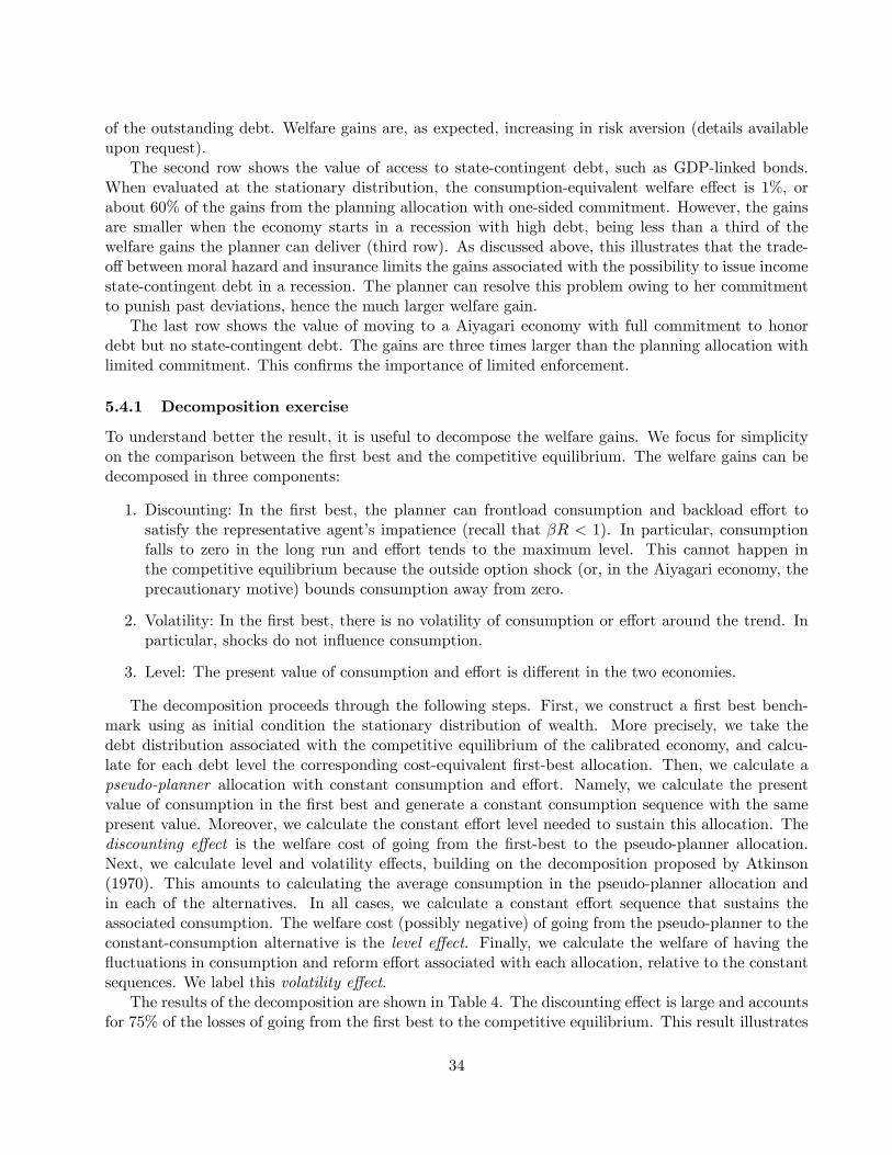
of the outstanding debt. Welfare gains are, as expected, increasing in risk aversion (details availableupon request).

The second row shows the value of access to state-contingent debt, such as GDP-linked bonds.When evaluated at the stationary distribution, the consumption-equivalent welfare e¤ect is 1%, orabout 60% of the gains from the planning allocation with one-sided commitment. However, the gainsare smaller when the economy starts in a recession with high debt, being less than a third of thewelfare gains the planner can deliver (third row). As discussed above, this illustrates that the trade-o¤ between moral hazard and insurance limits the gains associated with the possibility to issue incomestate-contingent debt in a recession. The planner can resolve this problem owing to her commitmentto punish past deviations, hence the much larger welfare gain.

The last row shows the value of moving to a Aiyagari economy with full commitment to honordebt but no state-contingent debt. The gains are three times larger than the planning allocation withlimited commitment. This con�rms the importance of limited enforcement.

5.4.1 Decomposition exercise

To understand better the result, it is useful to decompose the welfare gains. We focus for simplicityon the comparison between the �rst best and the competitive equilibrium. The welfare gains can bedecomposed in three components:

1. Discounting: In the �rst best, the planner can frontload consumption and backload e¤ort tosatisfy the representative agent�s impatience (recall that �R < 1). In particular, consumptionfalls to zero in the long run and e¤ort tends to the maximum level. This cannot happen inthe competitive equilibrium because the outside option shock (or, in the Aiyagari economy, theprecautionary motive) bounds consumption away from zero.

2. Volatility: In the �rst best, there is no volatility of consumption or e¤ort around the trend. Inparticular, shocks do not in�uence consumption.

3. Level: The present value of consumption and e¤ort is di¤erent in the two economies.

The decomposition proceeds through the following steps. First, we construct a �rst best bench-mark using as initial condition the stationary distribution of wealth. More precisely, we take thedebt distribution associated with the competitive equilibrium of the calibrated economy, and calcu-late for each debt level the corresponding cost-equivalent �rst-best allocation. Then, we calculate apseudo-planner allocation with constant consumption and e¤ort. Namely, we calculate the presentvalue of consumption in the �rst best and generate a constant consumption sequence with the samepresent value. Moreover, we calculate the constant e¤ort level needed to sustain this allocation. Thediscounting e¤ect is the welfare cost of going from the �rst-best to the pseudo-planner allocation.Next, we calculate level and volatility e¤ects, building on the decomposition proposed by Atkinson(1970). This amounts to calculating the average consumption in the pseudo-planner allocation andin each of the alternatives. In all cases, we calculate a constant e¤ort sequence that sustains theassociated consumption. The welfare cost (possibly negative) of going from the pseudo-planner to theconstant-consumption alternative is the level e¤ect. Finally, we calculate the welfare of having the�uctuations in consumption and reform e¤ort associated with each allocation, relative to the constantsequences. We label this volatility e¤ect.

The results of the decomposition are shown in Table 4. The discounting e¤ect is large and accountsfor 75% of the losses of going from the �rst best to the competitive equilibrium. This result illustrates

34

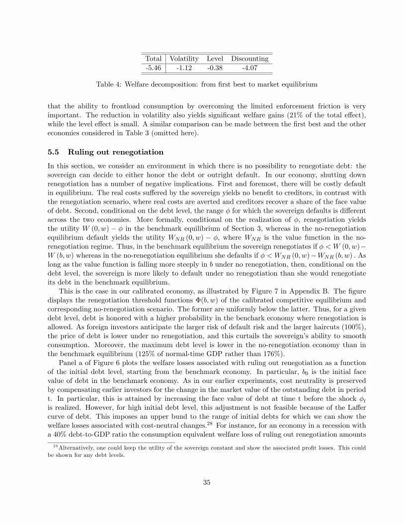
Total Volatility Level Discounting-5.46 -1.12 -0.38 -4.07

Table 4: Welfare decomposition: from �rst best to market equilibrium

that the ability to frontload consumption by overcoming the limited enforcement friction is veryimportant. The reduction in volatility also yields signi�cant welfare gains (21% of the total e¤ect),while the level e¤ect is small. A similar comparison can be made between the �rst best and the othereconomies considered in Table 3 (omitted here).

5.5 Ruling out renegotiation

In this section, we consider an environment in which there is no possibility to renegotiate debt: thesovereign can decide to either honor the debt or outright default. In our economy, shutting downrenegotiation has a number of negative implications. First and foremost, there will be costly defaultin equilibrium. The real costs su¤ered by the sovereign yields no bene�t to creditors, in contrast withthe renegotiation scenario, where real costs are averted and creditors recover a share of the face valueof debt. Second, conditional on the debt level, the range � for which the sovereign defaults is di¤erentacross the two economies. More formally, conditional on the realization of �, renegotiation yieldsthe utility W (0; w) � � in the benchmark equilibrium of Section 3, whereas in the no-renegotiationequilibrium default yields the utility WNR (0; w) � �; where WNR is the value function in the no-renegotiation regime. Thus, in the benchmark equilibrium the sovereign renegotiates if � < W (0; w)�W (b; w) whereas in the no-renegotiation equilibrium she defaults if � < WNR (0; w)�WNR (b; w) : Aslong as the value function is falling more steeply in b under no renegotiation, then, conditional on thedebt level, the sovereign is more likely to default under no renegotiation than she would renegotiateits debt in the benchmark equilibrium.

This is the case in our calibrated economy, as illustrated by Figure 7 in Appendix B. The �guredisplays the renegotiation threshold functions �(b; w) of the calibrated competitive equilibrium andcorresponding no-renegotiation scenario. The former are uniformly below the latter. Thus, for a givendebt level, debt is honored with a higher probability in the benchark economy where renegotiation isallowed. As foreign investors anticipate the larger risk of default risk and the larger haircuts (100%),the price of debt is lower under no renegotiation, and this curtails the sovereign�s ability to smoothconsumption. Moreover, the maximum debt level is lower in the no-renegotiation economy than inthe benchmark equilibrium (125% of normal-time GDP rather than 176%).

Panel a of Figure 6 plots the welfare losses associated with ruling out renegotiation as a functionof the initial debt level, starting from the benchmark economy. In particular, b0 is the initial facevalue of debt in the benchmark economy. As in our earlier experiments, cost neutrality is preservedby compensating earlier investors for the change in the market value of the outstanding debt in periodt. In particular, this is attained by increasing the face value of debt at time t before the shock �tis realized. However, for high initial debt level, this adjustment is not feasible because of the La¤ercurve of debt. This imposes an upper bund to the range of initial debts for which we can show thewelfare losses associated with cost-neutral changes.28 For instance, for an economy in a recession witha 40% debt-to-GDP ratio the consumption equivalent welfare loss of ruling out renegotiation amounts

28Alternatively, one could keep the utility of the sovereign constant and show the associated pro�t losses. This couldbe shown for any debt levels.

35

to 1.67% of permanent consumption. As a general pattern, the welfare losses are increasing in theinitial debt level and the sovereign�s risk aversion. This is not suprising, as the set of states in whichrenegotiation prevents costy default is larger when debt is large. Therefore, ruling out renegotiationis especially costly when an economy is in a recession with high debt.

5.6 Austerity cum Grexit

In this section, we evaluate the welfare consequences of an austerity program, where any violationof the program�s conditions triggers an immediate and permanent termination of the arrangement.This scenario is reminiscent of the so-called Grexit threat that was supported by some Eurozoneleaders, most notably the German Finance Minister Wolfgang Schäuble, before the third bailout planfor Greece was �nally settled in July 2015.29

Consider a once-and-for-all intervention of an external institution (the Trojka) that provides aguarantee on the sovereign�s obligations, so that the market price of debt will be 1=R in all states.The Trojka requires in exchange �scal austerity, i.e., the sovereign can roll over the outstandingdebt, but cannot borrow additional resources on the market. E¤ort is observable, and the Trojka iscommitted to terminate the assistance program (Grexit) as soon as the sovereign either attempts torenegotiate the outstanding debt, or violates the �scal austerity requirement. The abrupt terminationof the contract triggers default: the sovereign pays the cost � and does not repay its outstanding debt.Even in this case, the Trojka carries the loss and reimburses the investors for the debt issued beforedefault. In case of no termination, the program continues until the recession ends and (unless defaultoccurs right in the period in which the recession ends) no default cost ever becomes due. In this case,as the recession ends, the sovereign repays its debt and start borrowing at market terms.

This program has some attractive features: (i) the international guarantee reduces the burden ofservicing debt; (ii) the intervention mitigates the hold up problem in reform e¤ort. However, the �scalausterity requirement limits the possibility of borrowing to smooth consumption. Moreover, ine¢ cientterminations can occur inducing losses for the Trojka, and �uctuations in consumption and e¤ort ofthe borrowing country.

Panel b of Figure 6 plots the welfare losses arising from the introduction of the austerity programstarting from a competitive equilibrium. When the program starts, the Trojka purchases the out-standing debt at market value. Thereafter, it o¤ers the guarantee described above. Since a costlytermination may occur in equilibrium, the Trojka makes losses in expectations when entering theagreement. Therefore, the initial debt of the sovereign must be increased in order to retain cost neu-trality. Like in panel a, the La¤er curve of debt imposes an upper bound to the feasible initial debt.Therefore, we can only show welfare losses in the range below that debt level.

The welfare loss is decreasing in the outstanding debt, being as large as 0.97% at an initial debt-GDP ratio of 40% and 0.34% at an initial debt-GDP ratio of 100%. Intuitively, the higher the debtthe more severe the moral hazard in reform e¤ort and the less binding is �scal austerity (since thecost of raising funds in the market would be large in the competitive equilibrium). The value of theprogram increases with the risk tolerance. The dashed line in Figure 6 shows that when = 1 theimprovements in the moral hazard problem close to outweigh the other ine¢ ciencies of the interventionfor high debt levels.

In summary, the two last sections establish the two institutional arrangements that are often

29See, e.g., Spiegel online July 17, 2015, http://www.spiegel.de/international/germany/schaeuble-pushed-for-a-grexit-and-backed-merkel-into-a-corner-a-1044259.html.

36

0 0.05 0.1 0.15 0.2 0.25 0.3Initial debt, b

0

­3.5

­3

­2.5

­2

­1.5

­1

­0.5

Con

sum

ptio

n eq

uiva

lent

 wel

fare

 loss

 (%

)

(a) No Renegotiation

=1=2=3

0 0.1 0.2 0.3 0.4 0.5 0.6 0.7Initial debt, b

0

­2.5

­2

­1.5

­1

­0.5

0(b) Grexit

=1=2=3

Figure 6: Welfare losses of simple policies

praised in the policy debate for allegedly providing better ex-ante incentives, i.e., commitment not torenegotiate and �scal austerity, may be ine¢ cient. In our model, ruling out renegotiation is a badidea, whereas Grexit-style �scal austerity programs have ambiguous welfare e¤ects. Moreover, thee¤ects are negative in the calibrated economy. Both policies are dominated in welfare terms by thelaissez-faire arrangement, and a fortiori by an assistance program that allows repeated renegotiations(an approach that is reminiscent of the policy that was followed by the Trojka and that has often beenridiculed as inconsistent in the public debatea).

6 Conclusions

This paper presents a theory of sovereign debt dynamics under limited commitment. A sovereign coun-try issues debt to smooth consumption during a recession whose duration is uncertain and endogenous.The expected duration of the recession depends on the intensity of (costly) structural reforms. Bothelements � the risk of repudiation and the need for structural reforms �are salient features of therecent European debt crisis.

The competitive equilibrium, assumed to be Markovian, features repeated debt renegotiations.Renegotiations are more likely to occur during recessions and when the country has accumulated ahigh level of debt. As a recession drags on, the country has an incentive to go deeper into debt. Ahigher level of debt in turn may obstruct rather than encourage economic reforms.

The theory bears normative predictions that are relevant for events such as the European crisis.The competitive equilibrium is ine¢ cient for two reasons. On the one hand, due to the lack ofcommitment of market institutions, structural reforms are subject to a hold up problem. The intuitivereason is that the short-run cost of reforms is borne entirely by the country, while future bene�ts ofreforms accrue in part to the creditors in the form of an ex-post increased price of debt, due to areduction in the probability of renegotiation. On the other hand, the limited commitment to honor

37

debt induces high risk premia and excess consumption volatility. A well-designed intervention by aninternational institution endowed with commitment power can improve welfare. The optimal policyentails an assistance program whereby an international organization provides the country with aconstant transfer �ow, deferring the repayment of debt to the time when the recession ends. Theoptimal contract takes into account that this payment is itself subject to renegotiation risk.

The result that institutions endowed with commitment power can improve on the competitiveequilibrium hinges on reforms being observable, an assumption that is also maintained in the compet-itive equilibrium. If institutions cannot observe reform (even imperfectly), institutional commitmentis powerless, and the assistance program cannot improve on the competitive equilibrium. Arguably,in the recent debt crises, many reforms were by-and-large observable (e.g., labor market reforms, orthe establishment of a property registry in Greece), suggesting that commitment issues played animportant role.

A second implication is that, when the sovereign credibly threatens to renege on an existingagreement, concessions should be made to avoid an outright repudiation. Contrary to a commonperception among policy makers, a rigid commitment to enforce the terms of the original agreementis not optimal. Rather, the optimal policy entails the possibility of multiple renegotiations, which arere�ected in the terms of the initial agreement. Likewise, we show that shutting down renegotiationsis not useful, and induces instead additional welfare losses.

To retain tractability, we make important assumptions that we plan to relax in future research.First, in our theory the default cost follows an exogenous stochastic process. In a richer model, thiswould be part of the equilibrium dynamics. Strategic delegation is a potentially important extension.In the case of Greece, voters may have an incentive to elect a radical sovereign with the aim ofdelegating the negotiation power to an agent that has or is perceived to have a lower default costthan voters do (cf. Rogo¤ 1985). In our current model, however, the stochastic process governing thecreditor�s outside option is exogenous, and is outside of the control of the sovereign and creditors.

Second, again for simplicity, we assume that renegotiation is costless, that creditors can perfectlycoordinate and that they have full bargaining power in the renegotiation game. Each of these assump-tions could be relaxed. For instance, in reality the process of negotiation may entail costs. Moreover,as in the recent contention between Argentina and the so-called vulture funds, some creditors may holdout and refuse to accept a restructuring plan signed by a syndicate of lenders. Finally, the countrymay retain some bargaining power in the renegotiation. All these extensions would introduce interest-ing additional dimensions, and invalidate some of the strong e¢ ciency results (for instance, the resultthat the market economy attains the constrained optimum in the absence of income �uctuations).However, we are con�dent that the gist of the results is robust to these extensions.

Finally, by focusing on a representative agent, we abstract from con�icts of interest betweendi¤erent groups of agents within the country. Studying the political economy of sovereign debt wouldbe an interesting extension. We leave the exploration of these and other avenues to future work.

References

Abraham, Arpad, Eva Carceles-Poveda, and Ramon Marimon (2014). �On the optimal design of a �nancialstability fund,�Mimeo, European University Institute.

Aguiar, Mark, and Manuel Amador (2013). �Take the Short Route: How to Repay and Restructure SovereignDebt with Multiple Maturities,�NBER Working Paper No. 19717.

Aguiar, Mark, and Manuel Amador (2014). �Sovereign debt: a review,�Handbook of International Economics4, 647-87.

38

Aguiar, Mark, and Gita Gopinath (2006). �Defaultable Debt, Interest Rates, and the Current Account,�Journal of International Economics 69 (1), 64�83.

Alvarez, Fernando, and Urban J. Jermann (2000). �E¢ ciency, equilibrium, and asset pricing with risk ofdefault,�Econometrica 68(4), 775�797.

Angeletos, George-Marios (2002). �Fiscal Policy with Non-Contingent Debt and the Optimal Maturity Struc-ture,�Quarterly Journal of Economics 117(3), 1105-1131.

Arellano, Cristina (2008). �Default risk and income �uctuations in emerging economies,�American EconomicReview 98(3), 690�712.

Arellano, Cristina, Lilia Maliar, Serguei Maliar, and Viktor Tsyrennikov (2014). �Envelope Condition Methodwith an Application to Default Risk Models,�Mimeo, http://dx.doi.org/10.2139/ssrn.2470009.

Asonuma, Tamon, and Christoph Trebesch (2016). �Sovereign debt restructurings: preemptive or post-default,�Journal of the European Economic Association.

Atkeson, Andrew (1991). �International Lending with Moral Hazard and Risk of Repudiation,�Econometrica59(4), 1069-1089.

Atkinson, Anthony B. (1970). �On the Measurement of Inequality,�Journal of Economic Theory 2(3), 244-263.

Barro, Robert and David Gordon (1983). �Rules, discretion, and reputation in a model of monetary policy,�Journal of Monetary Economics 12(1), 101-121.

Benjamin, David, and Mark L. J. Wright (2009). �Recovery Before Redemption: A Theory of Delays inSovereign Debt Renegotiations,�Mimeo, State University of New York Bu¤alo.

Benveniste, Larry M., and Jose A. Scheinkman (1979). �On the Di¤erentiability of the Value Function inDynamic Models of Economics,�Econometrica 47(3), 727�732.

Blanchard, Olivier, and Francesco Giavazzi (2003). �Macroeconomic E¤ects of Regulation and Deregulationin Goods and Labor Markets,�Quarterly Journal of Economics 118(3), 879�907.

Boeri, Tito (2005). �Reforming labor and product markets: Some lessons from two decades of experiments inEurope,�IMF WP/05/97.

Bolton, Patrick, and Olivier Jeanne (2007). �Structuring and restructuring sovereign debt: the role of abankruptcy regime,�Journal of Political Economy 115(6), 901�924.

Borensztein, Eduardo, and Ugo Panizza (2009). �The costs of sovereign default,� IMF Sta¤ Papers 56 (4),683-741.

Broner, Fernando A., Guido Lorenzoni, and Sergio L. Schmukler (2013). �Why Do Emerging EconomiesBorrow Short Term?�Journal of the European Economic Association 11(1), 67�100.

Broner, Fernando A., Alberto Martin, and Jaume Ventura (2010). �Sovereign risk and secondary markets,�American Economic Review 100(4), 1523-1555.

Broner, Fernando A., and Jaume Ventura (2011). �Globalization and risk sharing,� Review of EconomicStudies 78(1), 49-82.

Brutti, Filippo, and Philip U. Sauré (2016). �Repatriation of Debt in the Euro Crisis,�Journal of the EuropeanEconomic Association 14(1).

Bulow, Jeremy, and Kenneth Rogo¤ (1989). �A constant recontracting model of sovereign debt,� Journal ofPolitical Economy 97(1), 155�178.

Bulow, Jeremy, and Kenneth Rogo¤ (2015). �Why sovereigns repay debts to external creditors and why itmatters,�Vox CEPR�s Policy Portal, June 10, 2015.

Clausen, Andrew, and Carlo Strub (2013). �A General and Intuitive Envelope Theorem,�Mimeo. Universityof Edinburgh, URL:https://andrewclausen.net/Clausen_Strub_Envelope.pdf.

39

Cole, Harold L., and Timothy J. Kehoe (1996). �A self-ful�lling model of Mexico�s 1994�1995 debt crisis,�Journal of International Economics 41(3), 309�330.

Cole, Harold L., and Timothy J. Kehoe (2000). �Self-ful�lling debt crises,�Review of Economic Studies 67(1),91�116.

Collard, Fabrice, Michel Habib, and Jean-Charles Rochet (2015). �Sovereign Debt Sustainability in AdvancedEconomies,�Journal of the European Economic Association 13(3), 381-420.

Conesa, Juan Carlos, and Timothy J. Kehoe (2015). �Gambling for redemption and self-ful�lling debt crises,�Research Department Sta¤ Report 465, Federal Reserve Bank of Minneapolis.

Cruces, Juan J., and Christoph Trebesch (2013). �Sovereign Defaults: The Price of Haircuts,� AmericanEconomic Journal: Macroeconomics 5(3), 85-177.

Dovis, Alessandro (2016). �E¢ cient Sovereign Default,�Mimeo, Pennsylvania State University.

Eaton, Jonathan, and Raquel Fernandez (1995). �Sovereign debt,�Handbook of International Economics 3,1243-2107.

Eaton, Jonathan, and Mark Gersovitz (1981). �Debt with potential repudiation: Theoretical and empiricalanalysis,�Review of Economic Studies 48(2), 289�309.

Fernandez, Raquel, and Robert W. Rosenthal (1989). �Sovereign-debt renegotiations revisted,�Working PaperNo. 2981, National Bureau of Economic Research.

Hopenhayn, Hugo and Ivan Werning (2008). �Equilibrium default,�Mimeo, MIT.

Ilzkovitz Fabienne, and Adriaan Dierx (2011). �Structural Reforms: A European Perspective,� Re�ets etperspectives de la vie économique 3/2011 (Tome L), 13�26.

Jeanne, Olivier (2009). �Debt Maturity and the International Financial Architecture,�American EconomicReview, 99(5), 2135�2148.

Kehoe, Patrick J., and Fabrizio Perri (2002). �International business cycles with endogenous incompletemarkets,�Econometrica 70(3), 907�928.

Kocherlakota, Narayana R. (1996). �Implications of e¢ cient risk sharing without commitment,�Review ofEconomic Studies 63(4), 595�609.

Krueger, Dirk, and Harald Uhlig (2006). �Competitive risk sharing contracts with one-sided commitment,�Journal of Monetary Economics 53(7), 1661�1691.

Krugman, Paul (1988). �Financing vs. forgiving a debt overhang,�Journal of Development Economics 29(3),253�268.

Ljungqvist, Lars, and Thomas J. Sargent (2012). Recursive Macroeconomic Theory, Third Edition, Cambridge,MA: MIT Press.

Mendoza, Enrique G., and Vivian Z. Yue (2012). �A General Equilibrium Model of Sovereign Default andBusiness Cycles,�Quarterly Journal of Economics 127(2), 889�946.

Müller, Andreas, Kjetil Storesletten, and Fabrizio Zilibotti (2016). �The Political Color of Fiscal Responsibil-ity,�Journal of the European Economic Association 14(1).

Panizza, Ugo, Federico Sturzenegger, and Jeromin Zettelmeyer (2009). �The economics and law of sovereigndebt and default,�Journal of Economic Literature 47(3), 651�698.

Prescott, Edward C., and Robert M. Townsend (1984). �General Competitive Analysis in an Economy withPrivate Information,�International Economic Review 25(1), 1�20.

Reinhart, Carmen M., and Kenneth S. Rogo¤ (2010). �From Financial Crash to Debt Crisis,�NBER WorkingPaper 15795.

Reinhart, Carmen M., and Christoph Trebesch (2016). �Sovereign debt relief and its aftermath,�Journal ofthe European Economic Association 14(1).

40

Renner, Philipp, and Karl Schmedders (2015). �A polynomial optimization approach to principal-agent prob-lems,�Econometrica 83(2), 729�769.

Rogo¤, Kenneth (1985). �The optimal degree of commitment to an intermediate monetary target,�QuarterlyJournal of Economics, 100(4), 141�182.

Song, Zheng, Kjetil Storesletten, and Fabrizio Zilibotti (2012). �Rotten Parents and Disciplined Children: APolitico-Economic Theory of Public Expenditure and Debt,�Econometrica 80(6), 2785�2803.

Spear, Stephen E., and Sanjay Srivastava (1987). �On repeated moral hazard with discounting,�Review ofEconomic Studies 54 (4), 599�617.

Stokey, Nancy L., and Robert E. Lucas, with Edward C. Prescott. 1989. Recursive Methods in EconomicDynamics. Publisher: Harvard University Press, Cambridge, Mass.

Sturzenegger, Federico, and Jeromin Zettelmeyer (2008). �Haircuts: estimating investor losses in sovereigndebt restructurings, 1998�2005,�Journal of International Money and Finance 27(5), 780�805.

Thomas, Jonathan, and Tim Worrall (1988). �Self-enforcing wage contracts,�The Review of Economic Studies55(4), 541�554.

Thomas, Jonathan, and Tim Worrall (1990). �Income �uctuation and asymmetric information: An exampleof a repeated pincipal-agent model,�Journal of Economic Theory 51(2), 367�390.

Tomz, Michael, and Mark L.J. Wright (2007). �Do countries default in bad times?,�Journal of the EuropeanEconomic Association 5(2-3), 352�360.

Yue, Vivian Z. (2010). �Sovereign default and debt renegotiation,�Journal of International Economics 80(2),176�187.

41

Online Appendixes of�Sovereign Debt and Structural Reforms�

Andreas Müller, Kjetil Storesletten and Fabrizio Zilibotti

A Appendix A: Proofs of lemmas, propositions, and corollaries.

Proof of Proposition 1. The case of normal times is straightforward. Consider an economystarting in a recession. Perfect insurance implies constant consumption and e¤ort. The e¢ cientsolution maximizes the discounted utility, W = u (c) = (1� �)�X (p) = (1� � (1� p)) with respect toc and p, subject to the following intertemporal budget constraint:

1

1� � (1� p) (w � c) +�

1� �p

1� � (1� p) ( �w � c) = b: (44)

Note that since insurance is provided in actuarially fair markets the budget constraint holds in expectedterms. Writing the Lagrangian, and di¤erentiating it with respect to c yields u0 (c) = �: Di¤erentiatingthe Lagrangian with respect to p and simplifying terms yields

X 0 (p)

�1� ��

+ p

��X (p) = ( �w � w)� u0 (c) ; (45)

which is identical to Equation (1) in the text. Equation (44) de�nes a positively sloped locus in theplane (p; c) ; while Equation (45) de�nes a negatively sloped locus in the same plane. Unless thesolution for e¤ort is a corner, the two equations pin down a unique interior solution for p and c.Consider the comparative statics with respect to b (note that b only features in equation (44)). Anincrease in b yields a decrease in c and an increase in p. This concludes the proof.

Proof of Lemma 1. The �rst part follows from the de�nitions of � and b̂. For the second part, notethat � (b; w) =W (0; w)�W (b; w) such that if W (b; w) is strictly decreasing in b, then � (b; w) mustbe strictly increasing in b. Thus, the inverse function of � (b; w) exits and is given by the expressionsstated in Lemma 1.

Proof of Proposition 2. We prove the existence of the Markov equilibrium by showing that thevalue function W is a �xed-point of a monotone mapping following Stokey and Lucas (1989, Theorem17.7).

Let �(w) be the space of bounded, continuous, and decreasing functions de�ned over [b;~b]. More-over, let d1 denote the supremum norm such that (�; d1) is a complete metric space. Let z 2 �(w)and be a real constant representing the outside option under outright default. T (z; ) is similar tothe Bellman equation of the Markov equilibrium in the text, but di¤ers in that the value of outright

I

default in the recession state is exogenously given by � �. We �rst establish the existence of anequilibrium for an exogenous ; and then extend the argument to an endogenous outside option as inthe Markov equilibrium.

De�ne the following mapping:

T (z; ;w) (b) = maxb02[b;~b]

u(Q(b0; z; )b0 � b+ w) + Z(b0; z; ; w); (46)

where � (x; z; ) = � z(x); and z�b̂ (�; z; )

�= � �: In addition, let T 0(z; ) = z, Tn(z; ) =

T (Tn�1(z; ); ), n = 1; 2; : : : , and zn � Tn(z; ). Moreover, when w = �w,

Z(x; z; ; �w) = �E�max

�z (x) ; � �0

�; and

Q(x; z; ; �w)x = R�1Ehmin

nx; b̂(�; z; )

oi:

Correspondingly, when w = w

Z(x; z; ; w) = �X((x; z; )) + ��(x; z; )E

�max

�W (x; �w) ;W (0; �w)� �0

�+(1�(x; z; ))E

�max

�z (x) ; � �0

� �;

X 0((x; z; )) = �

�[1� F (� (x; �w))]W (x; �w)� [1� F (�(x; z; ))] z(x)

�;

Q(x; z; ; w)x = R�1E

24 (x; z; )minnx; b̂ (�; �w)

o+(1�(x; z; ))min

nx; b̂ (�; z; )

o 35 :Note that the mapping during recession, T (z; ;w) ; takes as given the existence of the equilibriumfunctionsW (b; �w) ; � (b; �w) and b̂ (�; �w) : This is legitimate because one can prove existence recursively,�rst for normal times and then in recession.

We de�ne upper and lower bounds for the value functions. More formally, WMIN � u(w)=(1 ��) � �max, and WMAX � u( �w)=(1 � �). It is straightforward to see that WMIN and WMAX are,respectively, lower and upper bounds to the present utility the country can attain in equilibrium.

We establish �rst that the operator T (z; ;w) (b) is a uniformly continuous, bounded and decreas-ing (in b) mapping of the function space � into itself. Continuity follows by the Theorem of theMaximum. Boundedness follows from the fact that utility is bounded because consumption, reforme¤ort, the support of the default cost, and the elements of � are bounded. Finally, to establish thatthe mapping T is decreasing in b note that, for any � > 0; T (z; ;w) (b+�) < T (z; ;w) (b) since

T (z; ;w) (b+�) = maxb02[b;~b]

u�Q(b0; z; ; w)b0 + w � (b+�)

�+ Z

�b0; z; ; w

�= u (Q(B (b+�; z; ; w) ; z; ; w) �B (b+�; z; ; w) + w � (b+�)) + Z (B (b+�; z; ; w) ; z; ; w)< u (Q (B (b+�; z; ; w) ; z; ; w) �B (b+�; z; ; w) + w � b) + Z (B (b+�; z; ; w) ; z; ; w)� u (Q (B (b; z; ; w) ; z; ; w) �B (b; z; ; w) + w � b) + Z (B (b; z; ; w) ; z; ; w) = T (z; ;w) (b) ;

where B(b; z; ; w) = argmaxb02[b;~b] u(Q(b0; z; ; w)b0 � b+ w) + Z(b0; z; ; w):

Next, we establish that the mapping T (z; ;w) is monotone in z, that its �xed-point z� (z; ;w) (b) =limn!+1 Tn (z; ;w) (b) exists, and that z� 2 �. To this aim, consider z; z+ 2 � with z (b) < z+ (b),

II

8b 2 [b;~b]. Since z and z+ are decreasing in b; implying that z+�b̂(�; z+; )

�= �� > z

�b̂(�; z+; )

�,

it follows immediately that b̂(�; z; ) < b̂(�; z+; ). Consequently, � (b; z; ) � � (b; z+; ) for allb 2 [b;~b], which in turn implies that Q(b; z; ; w) � Q(b; z+; ; w). Consider �rst the case of w = �w:

We establish that z+ > z , T (z+; ; �w) (b) > T (z; ; �w) (b) ; since

T�z+; ; �w

�(b) = max

b02[b;~b]u�Q(b0; z+; ; �w)b0 � b+ �w

�+ Z

�b0; z+; ; �w

�= u

�Q(B

�b; z+; ; �w

�; z+; ; �w) �B

�b; z+; ; �w

�� b+ �w

�+ Z

�B�b; z+; ; �w

�; z+; ; �w

�� u

�Q(B (b; z; ; �w) ; z+; ; �w) �B (b; z; ; �w)� b+ �w

�+ Z

�B (b; z; ; �w) ; z+; ; �w

�> u (Q(B (b; z; ; �w) ; z; ; �w) �B (b; z; ; �w)� b+ �w) + Z (B (b; z; ; �w) ; z; ; �w)

= maxb02[b;~b]

u(Q�b0; z; ; �w

�b0 + �w � b) + Z

�b0; z; ; �w

�= T (z; ; �w) (b) :

where the �rst inequality follows from the fact that B (b; z; ; �w) yields a lower utility relative to theoptimal B (b; z+; ; �w). The second inequality follows from the fact that Q (b; z; ; �w) � Q (b; z+; ; �w)for all b 2 [b;~b].

Consider, next, the case of w = w: Let E �V (b) � E [V (b; �; �w)] : We establish that z+ > z ,T (z+; ;w) (b) > T (z; ;w) (b) ; since

T�z+; ;w

�(b) = max

b02[b;~b]u�Q(b0; z+; )b0 � b+ w

�+ Z

�b0; z+;

�= u

�Q(B

�b; z+;

�; z+; ) �B

�b; z+;

�� b+ w

��X

��B�b; z+;

�; z+;

��+

�(B (b; z+; ) ; z+; )�E �V (B (b; z+; ))+

(1�(B (b; z+; ) ; z+; ))�E [max f � �; z+ (B (b; z+; ))g]

�� u

�Q(B (b; z; ) ; z+; ) �B (b; z; )� b+ w

��X ( (B (b; z; ) ; z; ))

+

�(B (b; z; ) ; z; )�E �V (B (b; z; ))+

(1�(B (b; z; ) ; z; ))�E [max f � �; z+ (B (b; z; ))g]

�> u (Q (B (b; z; ) ; z; ) �B (b; z; )� b+ w)�X ( (B (b; z; ) ; z; ))

+

�(B (b; z; ) ; z; )�E �V (B (b; z; ))+

(1�(B (b; z; ) ; z; ))�E [max f � �; z (B (b; z; ))g]

�= max

b02[b;~b]u(Q(b0; z; )b0 � b+ w) + Z(b0; z; ) = T (z; ) (b; w) ;

where the same logic as above applies.We have established that T (z; ;w) is a monotone mapping with the sup norm. This mapping is

an equicontinuous family (each function in � is uniformly continuous and the continuity is uniformfor all functions in �). Then, Stokey and Lucas (1989, Theorem 17.7) ensures that the �xed point ofT (z; ;w) exists, is an element of � and is given by z�(z; ;w) = limn!+1 Tn(z; ;w).

Thus far, we have proven the existence of at least one �xed point of the mapping T for anyexogenous outside option, 2 [WMIN ;WMAX ] : We now use a di¤erent �xed point argument toshow that, conditional on an initial z; there exists a unique �xed point that the outside optionsin normal times and recession are, respectively, �z ( �w) and

�z (w) with the following properties:

z� (z; �z ( �w) ; �w) (0) = �z ( �w) = WMAX and z� (z; �z (w) ; w) (0) = �z (w) 2 (WMIN ;WMAX) : Tosee why, note that, by the Theorem of the Maximum, z� (z; ;w) (b) = limn!+1 Tn (z; ;w) (b) iscontinuous in . Moreover, z� is bounded since z� (z; ;w) 2 [WMIN ;WMAX ]. Thus, the Brouwer

III

�xed-point theorem ensures that there exists a z 2 [WMIN ;WMAX ] such that z� (z; z; w) (0) = z. Since z� (z; z; w) (0) = z � � (0; z�; z), this is equivalent to say that, at each �xed point,� (0; z�; �z (w)) = 0: To prove uniqueness, we note then that �

�0; z� ;

�is monotone increasing

for all 2 [WMIN ;WMAX ] ; as the set of (potential) states of nature in which the outside optionis attractive expands when increases. Therefore, there exists a unique �xed point �z (w) suchthat � (0; z�; �z (w)) = 0. In particular in normal times �z ( �w) = W (0; �w) = WMAX : In recession, �z (w) =W (0; w) 2 (WMIN ;WMAX).

The results proven thus far allow us to claim the existence of an equilibrium value function Wsuch that W (b; w) = T (W ;W (0; w) ; w) (b) : The de�nition of the remaining equilibrium functionsfollow from De�nition 1. This establishes the existence of a Markov equilibrium. The continuity ofthe value function W (b; w) in b follows from the Theorem of the Maximum, and implies that alsothe equilibrium functions �; Q and are continuous in b: It is also straightforward to show that Wis strictly decreasing in b and, hence, that � (b; w) = W (0; w) �W (b; w) is strictly increasing in b:Finally, we claim that the bond revenue, Q(b0; w)b0, is (weakly) monotone increasing in b0: This followsfrom equations (6)�(8), the fact that � increasing in b; and from Lemma 1.

Next, we prove that B is monotone decreasing in b by applying Topkis�Theorem: To this aim,de�ne B(b; w) = argmaxb02[b;~b]O(b

0; b; w) where

O(b0; b; w) = u(Q(b0; w)b0 � b+ w) + �Z(b0; w): (47)

We �rst establish that the objective function O(b0; b; w) is supermodular in (b0; b), i.e., if b0H > b0L and

bH > bL, then, O(b0H ; bH ; w)�O(b0L; bH ; w) � O(b0H ; bL; w)�O(b0L; bL; w). To this aim, note that

u(Q(b0H ; w)b0H � bH + w)� u(Q(b0L; w)b0L � bH + w) (48)

� u(Q(b0H ; w)b0H � bL + w)� u(Q(b0L; w)b0L � bL + w):

This inequality follows from the concavity of the utility function and the fact thatQ (b; w) b is increasingwith b; implying that, for � > 0;

u0(Q(x;w)x� b+ w)� u0(Q(x+�; w) (x+�)� b+ w) � 0:

Rearranging terms in (48), and adding and subtracting continuation values on both sides of theinequality yields

u(Q(b0H ; w)b0H � bH + w)� u(Q(b0H ; w)b0H � bL + w)

+�Z(b0H ; w)� �Z(b0H ; w)� u(Q(b0L; w)b

0L � bH + w)� u(Q(b0L; w)b0L � bL + w)

+�Z(b0L; w)� �Z(b0L; w)

that is equivalent to O(b0H ; bH ; w)�O(b0H ; bL; w) � O(b0L; bH ; w)�O(b0L; bL; w): This establishes thatO(b0; b; w) is supermodular in (b0; b): Topkis�Theorem implies then that B(bH ; w) � B(bL; w). Thisconcludes the proof of Proposition 2.

IV

Corollary 1 Let the operator T be de�ned as in Equation (46). If, for w 2 fw; �wg; W (b; w) =

limn!1 Tn (WMIN ;W (b; w) ; w) (b) = limn!1 Tn (WMAX ;W (b; w) ; w) (b), then the Markov equilib-rium is unique (i.e., there exists a unique equilibrium value function W (b; w) satisfying De�nition1).

Proof of Corollary 1. The proof follows immediately from the Corollary to Theorem 17.7 in Stokeyand Lucas (1989).

Proof of Proposition 3. The proof is an application of the generalized envelope theorem in Clausenand Strub (2013) which allows for discrete choices (i.e., repayment or renegotiation) and non-concavevalue functions. Consider the program W (b; w) = maxb02[b;~b]O(b

0; b; w) where O is de�ned in equation(47). Theorem 1 in Clausen and Strub (2013) ensures that if we can �nd a di¤erentiable lower supportfunction (DLSF) for O; then O is di¤erentiable for all b0 2 B(w):

We start by proving the lemma for the case of w = w. The strategy of the proof involves �ndingDLSF for the equilibrium functions Q(b0; w)b0 and Z(b0; w). To this aim, we follow the strategy ofBenveniste and Scheinkman (1979), and consider the value function of a pseudo-borrower that choosesdebt issuance b0 = B (x;w) instead of the optimal b0 = B (b; w),fW (b; x; w) � u (Q (B (x;w) ; w)B (x;w)� b+ w) + Z (B (x;w) ; w) :

Note that fW is di¤erentiable and strictly decreasing in b: Since debt issuance is chosen suboptimally,it must be the case that fW (b; x; w) � W (b; w) with equality holding at x = b. Furthermore, letthe pseudo-borrower set the default threshold at the level e� (b; x; w) = W (0; w) �fW (b; x; w), wheree� (b; x; w) � � (b; w). Thus, the pseudo-borrower will �nd it optimal to renegotiate for a range of �larger than �(b; w). Note that e� (b; x; w) is di¤erentiable and strictly increasing in b: Thus, the inversefunction exists and is such that e��1x;w (�) � b̂(�;w) (where we de�ne e�x;w (b) � e� (b; x; w)).

Consider �rst the case in which w = w. Let

eO �b0; b; x; w� = u� eQ(b0; x; w)b0 � b+ w�+ eZ(b0; x; w);

where the pseudo bond revenue function is given by

eQ �b0; x; w� b0 =1

Re(b0; x) h1� F (e� �b0; x; �w�)i b0 + Z e�(b0; �w)

0

e��1x; �w(�)dF (�)!

+1

R(1� e(b0; x)) h1� F (e� �b0; x; w�i b0 + Z e�(b0;w)

0

e��1x;w(�)dF (�)!;

and the continuation value is given by

eZ(b0; x; w) = �X(e(b0; x)) + �24 e(b0; x)EmaxnfW (b0; x; �w) ;fW (0; x; �w)� �0o+(1� e(b0; x))EmaxnfW (b0; x; w) ;fW (0; x; w)� �0o

35 ;having de�ned e as

e(b0; x) = �X 0��10@�24 Emax

nfW (b0; x; �w);fW (0; x; �w)� �0o�Emax

nfW (b0; x; w);fW (0; x; w)� �0o351A :

V

Note that eQ; eZ and e are di¤erentiable in b0 since we established above thatfW and e� are di¤erentiable.Then, eO is a DLSF for O such that eO(b0; b; x; w) � O(b0; b; w) with equality (only) at b0 = x. Thus,

Theorem 1 in Clausen and Strub (2013) ensures that the objective function O (b0; b; w) is di¤erentiablein b0 at b0 = B (b; w) and that @O(b0; b; w)=@b0 = @ eO(b0; b; B (b; w) ; w)=@b0 = 0. In this case, a standard�rst-order condition yields

@u (Q(b0; w)b0 � b+ w)@b0

+@Z(b0; w)

@b0= 0:

Moreover, Lemma 3 in Clausen and Strub (2013) ensures that the functions W (b; w), Z(b; w),�(b; w), Q(b; w), and (b) are di¤erentiable and that a standard envelope condition applies, namely,

@Z(b0; w)

@b0= �

"(b0) [1� F (�(b0; �w))] @W (b0; �w)

@b0

+(1�(b0)) [1� F (�(b0; w))] @W (b0;w)@b0

#;

@W (b; w)

@b= �u0 (Q(B(b; w); w)B(b; w)� b+ w) < 0:

The proof for the case of w = �w follows the same strategy and is therefore omitted.

Proof of Lemma 2. In normal times, the bond revenue function can be written as

Q(b0; �w)b0 = R�1Eminnb0; b̂(�; �w)

o.

Note that the minimum function in the expectation operator is concave in b0. Since the sum of concave

functions is still concave, then also Enmin b0; b̂(�; �w)

omust be concave in b0. This implies that the

marginal bond revenue is falling in b0. Di¤erentiating Q(b0; �w)b0 with respect to b0 2 [b;~b] yields:

@ (Q(b0; �w)b0)

@b0= Q

�b0; �w

�+@

@b0

R�1

�1� F

����b0���

+ (Rb0)�1Z ��(b0)

0

���1 (�)� f (�) d�!� b0

= Q�b0; �w

��R�1b0f

����b0��� @

�� (b0)

@b0

+b0(Rb0)�1 ���1����b0��f����b0��

�@��� (b0)

@b0� 1

R

1

b0

Z ��(b0)

0

����1 (�)� f (�) d�

�| {z }

=Q(b0; �w)� 1R(1�F(��(b0)))

= R�1�1� F

����b0���

:

Proof of Proposition 4. The �rst-order condition of (10) for w = �w yields:

@

@b0�b0 �Q

�b0; �w

�� u0 (c) + @

@b0�EV

�b0; �w

�= 0;

VI

The function V has a kink at b0 = b̂ (�; �w) : Consider, �rst, the range of realizations � > �� (b) implyingthat b0 < b̂ (�; �w). Di¤erentiating V in this range yields:

@

@bV (b; �; �w) = �u0 [Q (B (b; �w) ; �w)�B (b; �w) + �w � b] :

Next, consider the region of renegotiation, � < �� (b) ; implying that b > b̂ (�; �w) : In this case,@@bV (b; �; w) = 0. Using the results above one obtains:

@

@bEV (b; �w) =

Z ��(b)

0

@

@bV (b; �; �w) dF (�) +

Z 1

��(b)

@

@bV (b; �; �w) dF (�)

= �Z 1

��(b)u0 [Q (B (b; �w) ; �w)�B (b; �w) + �w � b] dF (�)

= ��1� F

��� (b)

��� u0 [Q (B (b; �w) ; �w)�B (b; �w) + �w � b] (49)

Plugging this expression back into the FOC, and leading the expression by one period, yields

0 =@

@b0�b0 �Q

�b0; �w

�� u0 (c)� �

�1� F

����b0���

� u0�c0jH; �w

�:

Finally, recall that @@b fb�Q (b; �w)g =

1R

�1� F

��� (b)

��; as established in the proof of Lemma 2.

Thus, for F��� (b)

�< 1; the above equation is equivalent to the CEE (13) in the proposition.

Although the �rst-order condition is also satis�ed at b0 = �b; it is possible to show that this is neveran optimal solution as long as b < �b (details in Appendix B).

Consider, next, the properties of the equilibrium functions C and W: Using the de�nition of Cin Equation (11) and Lemma 2, standard algebra shows that C is continuously di¤erentiable and de-creasing, with derivative @C(b; �w)=@b = R�1

�1� F (�� (b))

�� 1 < 0: Since B(b; �w) = b; then B maps

the complete domain of b into itself, B( �w) = [b;�b]. Proposition 3 implies then that the value functionis di¤erentiable everywhere, and that the envelope condition @W (b; �w)=@b = �u0(C(b; �w)) applies.Di¤erentiating this condition with respect to b yields @2W (b; �w)= (@b)2 = �u00(C(b; �w))@C(b; �w)=@b =u00(C(b; �w))

�1�R�1

�1� F (�� (b))

��< 0: This establishes that the value function W is twice contin-

uously di¤erentiable and strictly concave. This concludes the proof of the proposition.

Proof of Proposition 5. We start by claiming that cFB (b; w) > C (b; w), where cFB (b; w) wasde�ned in Proposition 1 and C (b; w) denotes consumption in the market equilibrium when debt ishonored. To see why, note that @=@b

�WFB (b; w)

� @=@b fW (b; w)g. This follows from observing

that the di¤erence between WFB (b; w) and WFB (b+�; w) ; where � > 0; merely re�ects the utilityloss from a permanent reduction in consumption cFB (b; w) and (in recession) a permanent increasein e¤ort pFB (b). In contrast, in the market equilibrium a larger debt induces a higher volatility ofconsumption (recall that � (b; w) is monotone increasing in b �see Lemma 1 �so higher debt increasesthe probability of renegotiation) and (in recession) e¤ort. Since @=@b

�WFB (b; w)

= �u0

�cFB (b; w)

�and @=@b fW (b; w)g = �u0 (C (b; w)) ; then the claim that cFB (b; w) > C (b; w) follows.

Let �min � [u ( �w)� u ((1� �) ( �w � w))] = (1� �) and bPV � w + �1�� �w. The assumption in the

Proposition implies that F (�min) = 0 and bPV < �w: Consider �rst the range b � bPV : In this range,W (b; �w) = WFB (b; �w) : To see this, note that W (bPV ; �w) = u ( �w � (1� �) bPV ) = (1� �) = �min:

VII

Since by assumption F (�min) = 0, no renegotiation is possible for b � bPV , so the claim follows. Thetwo claims above and Proposition 1 imply that C (b; �w) = cFB (b; �w) > cFB (b; w) � C (b; w) in therange b � bPV : Consider next the range b 2 (bPV ;�b]: In this range, C (b; w) � 0 since debt exceeds themaximum present value of future income. In contrast, C (b; �w) > 0 since bPV < �w: We have thereforeestablished that C (b; �w) > C (b; w) for all b � �b:

Proof of Lemma 3. If in the initial period (but not later) the country can contract on e¤ort whileissuing new debt, the problem becomes

maxb0;p�

�u (c)�X (p�) + �p� � EV

�b0; �w

�+ � (1� p�)� EV

�b0; w

�:

Note that the next-period value function V is the same as in the benchmark problem with non-contractible e¤ort, since we are considering a one-period deviation. The �rst-order condition withrespect to p yields

0 =d

dp��Q�b0; w

�b0� u0 (c)�X 0 (p�) + �

�EV

�b0; �w

�� EV

�b0; w

��) X 0 (p�) =

hQ�b0; �w

�� Q̂

�b0; w

�ib0 � u0 (c)

+�

�Z 1

0V�b0; �0; �w

�dF (�)�

Z 1

0V�b0; �0; w

�dF (�)

�> �

�Z 1

0V�b0; �0; �w

�dF (�)�

Z 1

0V�b0; �0; w

�dF (�)

�; (50)

where the last equation follows from the facts that Q (b0; �w) > Q̂ (b0; w) ; and that

d

dp

�Q�b0; w

�b0=

d

dp

nhpQ�b0; �w

�+ (1� p) Q̂

�b0; w

�ib0o

=hQ�b0; �w

�� Q̂

�b0; w

�ib0:

The right-hand side of the inequality in Equation (50) is the optimal e¤ort in the benchmark casewith non-contractible e¤ort, given in Equation (14). This establishes the lemma.

Proof of Proposition 6. Consider, �rst, the range b 2 [0; b1). Di¤erentiate equation (14) withrespect to b0,

X00 ��b0��0�b0�= �

�Z 1

0

@

@b0V�b0; �0; �w

�dF (�)�

Z 1

0

@

@b0V�b0; �0; w

�dF (�)

�= ��

�1� F

����b0���

� u0�Q�B�b0; �w

�; �w��B

�b0; �w

�+ �w � b0

�(51)

+��1� F

���b0���

��Q�B�b0; w

���B

�b0; w

�+ w � b0

�Taking the limit of equation (51) as b0 ! 0 yields

X00( (0))0 (0) = � [1� F (� (0))]� [Q (B (0; w))�B (0; w) + w � 0]

���1� F

��� (0)

��� u0 [Q (B (0; �w) ; �w)�B (0; �w) + �w � 0]

= ��u0 (Q (B (0; w))�B (0; w) + w � 0)� u0 ( �w)

�> 0; (52)

VIII

where the last equation uses the facts that �� (0) = � (0) = F (0) = 0 and that during normal timesc = �w if b = 0. Note that during recession, the annualized present value of income is strictly smallerthan �w. Therefore, it can never be optimal to choose consumption during recession larger than orequal to �w when b = 0. Since the marginal utility of consumption is larger in a recession thanduring normal times, the right-hand side of Equation (52) is strictly positive. Since X 00 > 0, thenlimb!0

0 (b) = 0 (0) > 0. By continuity, it follows then that 0 (b) will be positive for a range of bclose to b = 0, so there must exist a b1 > 0 such that 0 (b) > 0 for all b 2 [0; b1).Consider, next, the range b 2

�b�;�b

�, in which case F (� (b)) = 1 and F

��� (b)

�< 1. This implies that

Equation (51) can be written as

X00( (b))0 (b) = ��

�1� F

��� (b)

��� u0 [Q (B (b; �w) ; �w)�B (b; �w) + �w � b] < 0;

which establishes that 0 (b) < 0 for all b 2�b�;�b

�and with strict inequality also for b = b�. By

continuity, it follows then that there exists a b2 < b� such that 0 (b) < 0 for all b 2�b2;�b

�. Finally,

in the range where b � �b, F (� (b)) = F��� (b)

�= 1 so the right-hand side of Equation (51) becomes

zero, implying that 0 (b) = 0.

Proof of Proposition 7. The procedure is analogous to the derivation of the CEE in normal times.The �rst-order condition of (10) for w = w yields

0 =d

db0�Q�b0; w

�� b0

� u0 (c) + �

�1�

�b0�� ddb0EV

�b0; w

�+ �

�b0� ddb0EV

�b0; �w

�;

where a term has been cancelled by the envelope theorem. Using the same argument as in the proofof Proposition 4 we can write:

d

dbEV (b; w) = � [1� F (� (b))]� u0 [Q (B (b; w) ; w)�B (b; w) + w � b] :

Plugging this back into the FOC (after leading the expression by one period) yields the CEE

0 = u0 (c)�n0�b0��R

hQ�b0; �w

�� Q̂

�b0; w

�ib0+

+ �b0���1� F

����b0���

+�1�

�b0����1� F

���b0���

��R��1�

�b0����1� F

���b0���

u0�c0jH;w

�+

�b0���1� F

����b0���

u0�c0jH; �w

��;

where the equality follows from Lemma 4. Rearranging terms yields Equation (16).

Proof of Lemma 4. Di¤erentiating the bond revenue with respect to b yields

d

dbfQ (b; w) bg =

d

db

npbQ (b; �w) + (1� p) bQ̂ (b; w)

o+0 (b)�

�Q (b; �w)� Q̂ (b; w)

�b

= (b)� 1

R

�1� F

��� (b)

��+ (1�(b))� 1

R(1� F (� (b))) (53)

+0 (b)��Q (b; �w)� Q̂ (b; w)

�b;

IX

where the second equality can be derived as following:

d

db

npbQ (b; �w) + (1� p) bQ̂ (b; w)

o= p

1

R

�1� F

��� (b)

��+ (1� p) Q̂ (b; w)

+ (1� p)"

� bRf (� (b))� �

0 (b)�1R1b

R �(b)0

���1 (�)� f (�) d�

�+ 1

Rbf (� (b))�0 (b)

#= p

1

R

�1� F

��� (b)

��+ (1� p) 1

R(1� F (� (b)))

Consider, �rst, the case in which (b) is constant, (b) = p: In this case, debt revenue is increasingfor all b < �b; since, then, p=R�

�1� F

��� (b)

��+(1� p) =R�(1� F (� (b))) > 0. Moreover, it reaches

a maximum at b = �b (recall that F��� (b)

�< F (� (b)) for all b < �b). This establishes that, if is

constant, then �bR = �b:Consider, next, the general case. Proposition 6 implies that, in the range where b 2 [b2;�b]; 0 (b) <

0: Since Q (b; �w) > Q̂ (b; w), then, in a left neighborhood of �b; 0 (b)�hQ (b; �w)� Q̂ (b; w)

ib < 0: This

means that, starting from �b; one can increase the debt revenue by reducing debt, i.e., �bR < �b:

Proof of Proposition 8. We proceed in two steps: �rst, we derive the CEEs (step A), and thenwe show that �

�b0w; b

0�w

�> 0 (step B).

Step A: The �rst-order conditions with respect to b0�w and b0w in problem (18) yields

0 = u0 (c)� d

db0�wREV

�b0w; b

0�w

�+ �

�b0w; b

0�w

� d

db0�wEV

�b0�w; �w

�;

0 = u0 (c)� d

db0wREV

�b0w; b

0�w

�+ �

�1�

�b0w; b

0�w

�� d

db0wEV

�b0w; w

�;

where REV�b0w; b

0�w

�� b0w�Qw

�b0w; b

0�w

�+ b0�w�Q �w

�b0w; b

0�w

�is the bond revenue and c is de�ned in the

Proposition. Note that both equations have been simpli�ed using an envelope condition. The valuefunction has a kink at b = b̂ (�;w) : Consider, �rst, the range of realizations � 2 [� (b) ;+1) ; implyingthat b < b̂ (�;w). Di¤erentiating the value function yields:

d

dbV (b; �; �w) = �u0 [Q (B (b; �w) ; �w)�B (b; �w) + �w � b] ;

d

dbV (b; �; w) = �u0

�Qw�Bw (b) ; B �w (b)

��Bw (b) +Q �w

�Bw (b) ; B �w (b)

��B �w (b) + w � b

�;

where Bw and B �w denote the optimal issuance of the two assets, respectively. Next, consider the rangeof realizations � < � (b) ; implying that b � b̂ (�;w). In this case, ddbV (b; �; w) = 0.

In analogy with equation (49), we obtain:

d

dbEV (b; w) = � [1� F (� (b))]� u0

�cjH;w

�: (54)

Plugging (49) and (54) into the respective �rst-order conditions, and leading by one period, yields

u0 (c)� d

db0�wREV

�b0w; b

0�w

�= �

�b0w; b

0�w

���1� F

����b0�w���

� u0�c0jH; �w

�;

X

u0 (c)� d

db0wREV

�b0w; b

0�w

�= �

�1�

�b0w; b

0�w

����1� F

���b0�w���

� u0�c0jH;w

�:

The marginal revenues from issuing recession-contingent debt is given by:

d

db0wREV

�b0w; b

0�w

�=

1��b0w; b

0�w

�R

�1� F

���b0w���

�@(b0w;b0�w)

@b0w

1��b0w; b

0�w

�Qw �b0w; b0�w�� b0w + b0�w � @

@b0wQ �w

�b0w; b

0�w

�=

1��b0w; b

0�w

�R

�1� F

���b0w���

+@�b0w; b

0�w

�@b0w

���b0w; b

0�w

�; (55)

where, note, @@b0wQ �w

�b0w; b

0�w

�=

@(b0w;b0�w)@b0w

Q �w(b0w;b0�w)(b0w;b0�w)

follows from applying standard di¤erentiation to the

de�nition of Q �w

�b0w; b

0�w

�in equation (21). Applying the same methodology to the recovery-contingent

debt, we obtain:

d

db0�wREV

�b0w; b

0�w

�=�b0w; b

0�w

�R

�1� F

����b0�w���

+@�b0w; b

0�w

�@b0�w

���b0w; b

0�w

�:

The CEEs conditional on the recession continuing and ending, respectively, are then:

�u0�c0jH;w

�u0 (c)

=1

R+

@

@b0w�b0w; b

0�w

��

��b0w; b

0�w

��1� F

���b0w��� �

1��b0w; b

0�w

���u0 (c0jH; �w)u0 (c)

=1

R+

@

@b0�w�b0w; b

0�w

��

��b0w; b

0�w

��1� F

��� (b0�w)

���b0w; b

0�w

� :Setting �R = 1 yields equations (22)-(23).

Step B: Next, we prove that, in equilibrium, ��b0w; b

0�w

�> 0. To prove the claim, it is useful to

de�ne the two functions

� �w�b0�w��

Q �w

�b0w; b

0�w

�� b0�w

�b0w; b

0�w

� =1

R

�1� F

����b0�w���

b0�w +

Z ��(b0�w)

0

���1 (�)� f (�) d�!;

�w�b0w��

Qw�b0w; b

0�w

�� b0w

1��b0w; b

0�w

� =1

R

�1� F

���b0w���

b0w +

Z �(b0w)

0��1 (�)� f (�) d�

!;

where, recall, � (x) > �� (x) and F (� (x)) > F��� (x)

�. Note that �

�b0w; b

0�w

�= � �w (b

0�w) � �w

�b0w�;

where both � �w and �w are increasing functions in the relevant range, i.e., b0�w � �b and b0w � �b. Weproceed in two steps. First, we show that �

�b0w; b

0�w

�� 0 ) b0�w > b

0w (step B1). Next, we show that

b0�w > b0w ) ��b0w; b

0�w

�> 0 (step B2). Steps B1 and B2 establish jointly a contradiction ruling out

that ��b0w; b

0�w

�� 0 (step B3).

Step B1: Suppose that ��b0w; b

0�w

�� 0. Then, the CEEs (22)�(23) and the assumption that

u00 < 0, imply thatc0jH; �w � c � c0jH;w: (56)

XI

Suppose, to derive a contradiction, that b0w � b0�w. Recall that, if the recession ends and debt is honored,debt remains constant, i.e., b

00= B (b0�w) = b

0�w. Moreover, Q (b

0�w; �w) = Q �w

�b0w; b

0�w

�=�b0w; b

0�w

�. Thus,

c0jH; �w = Q (b0�w; �w) b0�w + �w � b0�w = � �w (b0�w) + �w � b0�w.

c0jH; �w = �b0w; b

0�w

�� �w�b0�w�+�1�

�b0w; b

0�w

��� �w�b0�w�+ �w � b0�w

� �b0w; b

0�w

�� �w�b0�w�+�1�

�b0w; b

0�w

��� �w�b0w�+ �w � b0w

� �b0w; b

0�w

�� �w�b0�w�+�1�

�b0w; b

0�w

���w�b0w�+ �w � b0w

> �b0w; b

0�w

�� �w�b0�w�+�1�

�b0w; b

0�w

���w�b0w�+ w � b0w = c0jH;w:

The �rst inequality follows from the assumption that b0w � b0�w and the fact that (1� p) � �w (x)�x < 0 forany p 2 [0; 1], which is due to the fact that � �w (x) � x=R < x for any x. The second inequality followsfrom the fact that � �w

�b0w�� �w

�b0w�, see equation (57) below. The last inequality follows from the

maintained assumption that �w > w. We have therefore proven that if b0w � b0�w then c0jH; �w > c0jH;w,which contradicts (56) and, hence, implies that �

�b0w; b

0�w

�� 0. We conclude from Step B1 that

��b0w; b

0�w

�� 0) b0�w > b

0w.

Step B2: Suppose that b0w = b0�w = x: Then, for any x:

�(x; x) = � �w (x)� �w (x) =1

R

Z �(x)

��(x)

��x� ��1 (�)

�� f (�) d�

�| {z }

>0

(57)

+1

R

Z ��(x)

0

�����1 (�)� ��1 (�)

�� f (�) d�

�| {z }

>0

> 0:

Since � �w (x) is an increasing function for x � �b, equation (57) implies that � �w (b0�w) > �w�b0w�, for all

b0w < b0�w � �b. We conclude from Step B2 that b0�w > b

0w ) �

�b0w; b

0�w

�> 0.

Step B3: Putting together the conclusions of Step B1 and Step B2, we derive a contradiction:��b0w; b

0�w

�� 0) b0�w > b

0w ) �

�b0w; b

0�w

�> 0. Therefore, we must have that �

�b0w; b

0�w

�> 0:

Proof of Proposition 9. We write the Lagrangian,

�� =

Z@

��w � �c� +

1

R�P (�!�)

�dF (�) + ��

�Z@[u (�c�) + ��!�] dF (�)� �

�+

Z@��� [u (�c�) + ��!� �W (0; �w) + �] d�;

with the associated multipliers �� and ���. The �rst-order conditions yield

f (�) = u0 (�c�)���f (�) + ���

�; (58)�

��f (�) + �����R = � �P 0 (�!�) f (�) : (59)

The envelope condition yields� �P 0 (�) = �� (60)

XII

The two �rst-order conditions, the envelope condition and �R = 1 jointly imply that

u0 (�c�) = � 1�P 0 (�!�)

(61)

�P 0 (�!�) = �P 0 (�)����f (�)

: (62)

Note that (61) is equivalent to (28) in the text. Consider, next, two cases, namely, when the PC isbinding and when it is not binding.

When the PC is binding, ��� > 0: (62) implies then that �!� > �: Then, (61) and (29) determinejointly the solution for (�c�; �!�) : When the PC is not binding, ��� = 0: (62) implies then that �!� = �and �c� = �c (�) :

What remains to be shown is that the �rst-order conditions are su¢ cient. The proof followsThomas and Worrall (1990, Proof of Proposition 1). The details of this proof are in Proposition 16 inAppendix B.

Proof of Lemma 5. The Lagrangian of the planner�s problem reads as

� =

Z@

�w � c� +

1

R

�(1� p�)P

�!��+ p� �P (�!�)

��dF (�)

+�

�Z@

�u�c���X (p�) + �

�(1� p�)!� + p��!�

��dF (�)� �

�+

Z@���u�c���X (p�) + �

�(1� p�)!� + p��!�

�� � + �

�d�

+

Z@ ���X (p�) + �

�(1� p�)!� + p��!�

�� �dev

�d�;

where the Lagrange multipliers of the PC and IC must be non-negative for all �, �� � 0; � � 0. The�rst-order conditions in combination with �R = 1 yield:

f (�) = u0�c�� �� f (�) + ��

�; (63)

� f (�) + �� + � = �P 0�!��f (�) ; (64)

� f (�) + �� + � = � �P 0 (�!�) f (�) ; (65)

R�1��P (�!�)� P

�!���f (�) =

�� f (�) + �� + �

� �X 0 (p�)� �

��!� � !�

��; (66)

while the envelope condition yields�P 0 (�) = �: (67)

The �rst-order conditions (64)�(66) imply equations (34)-(35) in the text. Since P and �P aremonotonic and strictly concave, equation (34) implies a strictly positive relationship between !� and�!�. Equation (35) yields then a strictly negative relationship between p� and !�, and a strictlyincreasing relationship between p� and �!�. Consider, next, the IC constraint. Therefore, when the ICis binding, the binding constraint (33), (34), and (35) pin down a unique solution for p�; !� and �!�;denoted by (p�; !�; �!�).

XIII

Proof of Proposition 10. We start by showing that � � !� implies that the IC is never strictlybinding. Combine equations (64) and (67) to yield P 0 (�) � P 0

�!��. Since P is strictly concave this

implies that promised utility is non-decreasing, !� � �, conditional on staying in recession. Moreover,!� � � � !�, thus the IC is never strictly binding, � = 0. When � = 0, the FOCs in (64)�(66) read

u0�c��= � 1

P 0�!��

P 0�!��= P 0 (�)�

��f (�)

P 0�!��= �P 0 (�!�)

X 0 (p�) = u0 (c�)R�1 � �P (�!�)� P �!���+ � ��!� � !�� :

The solution will therefore depend on whether the PC is slack or binding:

1. When the PC is binding and the recession continues, � < ~�(�), �� > 0, !� > �, and

u�c���X (p�) + �

�(1� p�)!� + p��!�

�=W (0; w)� �: (68)

Then, (34), (35), (36) and (68) determine jointly the solution for�c�; p�; !�; �!�

�. In this case,

there is no history dependence, i.e., � does not matter.

2. When the PC is not binding, � � ~�(�) and �� = 0: Then, !� = �, and c� = c (�), p� = p(�),and �!� = �!�(�) are determined by (36), (34), and (35), respectively. The solution is historydependent. Equation (35) and �R = 1 imply that

u0 (c (�))��P (�! (�))� P (�)

�+ [�! (�)� �] = ��1X 0 (p (�)) ;

namely, the planner requires constant e¤ort over the set of states for which the constraint is notbinding: p� = p (�). Di¤erentiating the left-hand side yields

u00 (c (�)) c0 (�)���P (�! (�))� P (�)

�| {z }<0

+�u0 (c (�))P 0 (�) + 1

� ��!0 (�)� 1

�= u00 (c (�)) c0 (�)�

��P (�! (�))� P (�)

�< 0

since, recall, (36) implies that P 0 (�) = �1=u0 (c (�)). This implies that the right-hand side mustalso be decreasing in �. Since X is convex and increasing, this implies in turn that p (�) mustbe decreasing in �. Moreover, P 0 (�) = �1=u0 (c (�)), implies that c (�) must be increasing in �,while P 0 (�) = �P 0 (�!(�)) shows that also �!(�) is increasing in �.

This concludes the proof.

Proof of Proposition 11. This proof builds on the proof of Lemma 5 and Proposition 10. Wealready know that in the case � < !� the IC is potentially binding.

1. When the IC is not binding, � = 0, the solution (c�; p�; !�; �!�) is as described in Proposition10.

XIV

2. When the IC and the PC is binding, � > 0 and , �� > 0, then p� = p�; !� = !

�; �!� = �!� asdescribed in Lemma 5. Consumption varies with the realization of � and is determined by thebinding PC and IC in equations (32) and (33) which imply equation (38) in the proposition.

3. When the IC is binding and the PC is not binding, � > 0 and , �� = 0, then p� = p�; !� =

!�; �!� = �!� as described in Lemma 5. Consumption is constant across � and determined bythe binding promise-keeping constraint in (31). Alternatively, at the threshold realization ~�(�),consumption must be the same as in equation (38) which implies equation (39).

Finally, we guess and verify that the threshold realization of � where the IC starts binding is givenby �� = ~�(!�) � ~�(�). Consider the promise-keeping constraint when the current promised utility is� = !�:

!� =

Z ��

0

�u(c�)�X(p�) + �

�(1� p�)!� + p��!�

��dF (�)

+

Z �max

��

hu(c���) + �dev

idF (�)

=

Z ��

0[W (0; w)� �] dF (�) + (W (0; w)� ��) [1� F (��)]

= W (0; w)�Z ��

0�dF (�)� �� [1� F (��)] :

The comparison with the threshold function in (37) con�rms the guess that �� = ~�(!�).

Proof of Proposition 12. The planner solves (30) subject to (31), (32), and (40). We write theLagrangian,

� =

Z@

�w � c� +R�1

��1��(�!� � !�)

�P�!��+�(�!� � !�) �P (�!�)

��dF (�)

+�

�Z@

�u (c�)�X

��(�!� � !�)

�+ �

��1��(�!� � !�)

�!� +�(�!� � !�)�!�

��dF (�)� �

�+

Z@���u�c���X

��(�!� � !�)

�+ �

��1��(�!� � !�)

�!� +�(�!� � !�)�!�

��W (0; w) + �

�d�;

where � and �� denote the multipliers in recession. The �rst-order conditions with respect to c�, �!�,and !� yield

0 = �f(�) +��f(�) + ��

�u0(c�);

0 = R�1��(�!� � !�) �P 0 (�!�) + �0(�!� � !�)

��P (�!�)� P

�!����f(�)

+��f(�) + ��

� � �X 0(�(�!� � !�))�0(�!� � !�)+���(�!� � !�)1 + �0(�!� � !�)

��!� � !�

�� ��0 = R�1

��1��(�!� � !�)

�P 0�!��+�0(�!� � !�)(�1)

��P (�!�)� P

�!����f(�)

+��f(�) + ��

� � �X 0(�(�!� � !�))�0(�!� � !�)(�1)+���1��(�!� � !�)

�1 + �0(�!� � !�)(�1)

��!� � !�

�� � :XV

Moreover, the �rst-order condition for reform e¤ort reads

X 0(�(�!� � !�))� �(�!� � !�) = 0

and the envelope condition is given byP 0 (�) = ��:

Combining the �rst-order conditions and the envelope condition yields

1

u0(c�)= �P 0 (�) +

��f(�)

(69)

�R1

u0(c�)= �

��P 0 (�!�) +

�0(�!� � !�)�(�!� � !�)

��P (�!�)� P

�!����

(70)

�R1

u0(c�)= �

�P 0�!���

�0(�!� � !�)1��(�!� � !�)

��P (�!�)� P

�!����

: (71)

Given that �R = 1, Equations (70) and (71) imply that (41) and (42) must hold for any realizeddefault cost state �.

For all states � where the participation constraint is not binding, �� = 0, the �rst-order conditionin (69) satis�es

1

u0(c�)= �P 0 (�) : (72)

In that case, the solution is history dependent, c� = c(�), !� = !(�), �!� = �!(�) and determinedby (69), (41) and (42). For all states where the participation constraint is binding, �� > 0, theparticipation constraint holds

u�c���X

��(�!� � !�)

�+ �

� �1��(�!� � !�)

�!�

+�(�!� � !�)�!�

�=W (0; w)� �:

In that case, the solution c�, !�, �!� is independent of � and determined by the binding PC in (32),(41), and (42).

Finally, note that the threshold realization of � where the constraint starts binding, ~�(�), remainsdetermined by the binding promise-keeping constraint

� =

Z ~�(�)

0[W (0; w)� �] dF (�) +

Z �max

~�(�)

�u (c(�))�X (�(�!(�)� !(�)))

+� ((1��(�!(�)� !(�)))!(�) + �(�!(�)� !(�))�!(�))

�dF (�)

= W (0; w)�"Z ~�(�)

0�dF (�) +

h1� F (~�(�))

i~�(�)

#:

Thus, �� = 0, � � ~�(�) and �� > 0, � < ~�(�). This concludes the proof of the proposition.

Proof of Proposition 13. We prove the proposition by deriving a contradiction. To this aim,suppose that, for �� (b) = �P (�) ; the planner can deliver more utility to the agent than can the marketequilibrium. Namely, � > EV (b; �w). Then, since �P is a decreasing strictly concave function, we musthave that �P (EV (b; �w)) > �P (�) and �P 0 (EV (b; �w)) > �P 0 (�) :We show that this inequality, along withthe set of optimality conditions, induces a contradiction.

XVI

First, recall, that equation (6) implies that �� (b) = RQ (b; �w) b: Thus,

�P (EV (b; �w)) > �P (�) = RQ (b; �w) b; (73)

where EV (b; �w) is decreasing in b. Di¤erentiating the two sides of the inequality (73) with respect tob yields

�P 0 (EV (b; �w))� d

dbEV (b; �w) >

d

db[Q (b; �w) b]�R = 1� F

��� (b)

�; (74)

where the right-hand side equality follows from the proof of Lemma 2. Next, equation (49) impliesthat

d

dbEV (b; �w) = �

�1� F

��� (b)

��� u0 [C (b; �w)] ;

where C (b; �w) = Q (B (b; �w) ; �w)�B (b; �w)+ �w� b is the consumption level in the market equilibriumwhen the debt b is honored. Plugging the expression of d

dbEV (b; �w) into (74), and simplifying terms,yields

u0 (C (b; �w)) > � 1�P 0 (EV (b; �w))

: (75)

Next, note that C (b; �w) = �c (�) : Equation (75) yields u0 (�c (�)) > �1= �P 0 (EV (b; �w)) ; while (61)yields that u0 (�c (�)) = �1= �P 0 (�) : Thus, the two conditions jointly imply that �P 0 (�) > �P 0 (EV (b; �w))

which in turn implies that � < EV (b; �w), since �P is decreasing and concave. This contradicts theassumption that � > EV (b; �w) :

The analysis thus far implies that � � EV (b; �w) :We can also rule out that � < EV (b; �w), becauseit would contradict that the allocation chosen by the planner is constrained e¢ cient. Therefore,� = EV (b; �w) :

Proof of Proposition 14. The strategy of the proof is the same as that of Proposition 13. Weprove the proposition by deriving a contradiction. To this aim, suppose that, for �(b) = P (�) ; theplanner can deliver more utility than the agent gets in the market equilibrium. Namely, � > EV (b; w).Then, since P is a decreasing strictly concave function, we must have that P (EV (b; w)) > P (�) andP 0 (EV (b; w)) > P 0 (�) : Note that, absent moral hazard, the price of recession-contingent debt isindependent of the amount of recovery-contingent debt. It is therefore legitimate to de�ne ~Qw

�b0w��

Qw�b0w; b

0�w

�:

First, the same argument invoked in the proof of Proposition 13 implies that �(b) = R1�p

~Qw (b) b:

Hence,

P (EV (b; w)) > P (�) =R

1� p~Qw (b) b: (76)

where EV (b; w) is decreasing in b. Di¤erentiating the two sides of the inequality (76) with respect tob yields:

P 0 (EV (b; w))� d

dbEV (b; w) (77)

>R

1� pd

db

�~Qw (b) b

�= � [1� F (� (b))] ;

XVII

where the right-hand side equality follows from equation (55). Next, equation (49) implies that

d

dbEV (b; �w) = �

�1� F

��� (b)

��� u0 (C (b; �w)) ;

where C (b; w) is the consumption level assuming that the recession-contingent debt b is honored.Plugging in the expression of d

dbEV (b; �w) allows us to simplify (77) as follows:

u0 (C (b; w)) > � 1

P 0 (EV (b; w)): (78)

Next, note that C (b; w) = c (�) : Equation (78) yields u0 (c (�)) > � 1P 0(EV (b;w))

; while (72) yields

that u0 (c (�)) = � 1P 0(�)

: Thus, the two conditions jointly imply that � 1P 0(�)

> � 1P 0(EV (b;w))

which inturn implies that � < EV (b; w), since P is decreasing and concave. This contradicts the assumptionthat � > EV (b; w) :

The analysis thus far establishes that � � EV (b; w) : We can also rule out that � < EV (b; w) be-cause it would contradict that the allocation chosen by the planner is constrained e¢ cient. Therefore,� = EV (b; w).

Proof of Proposition 15. We have already shown in Proposition 13 that the market equilibriumis equivalent to the planner solution once the economy has entered the absorbing normal time state.Thus, we can limit the proof to the recession state. The strategy of the proof is to show that the�rst-order conditions of the planner problem and the market equilibrium are equivalent. Under ourassumption that the �rst-order conditions of the planner problem are necessary and su¢ cient for thecharacterization of the optimal contract, this proves that the market equilibrium decentralizes theplanner solution.

Let the solution of an interior state-contingent Markov equilibrium be denoted by the collectionof functions

EV (b; w); C(�; w);(�; �); B �w(�; w); Bw(�; w):This solution necessarily satis�es the government budget constraint in (17) and the necessary opti-mality conditions for reform e¤ort and debt issuance in Equations (19), (22), and (23). We show inthe following that an interior solution to the planner problem satis�es these optimality conditions andthe budget constraint. Formally, we guess and verify that

EV (b; w) = �

C�(b) � C(B(b; �; w); w) = c�(�)�(b) � (Bw(B(b; �; w); w); B �w(B(b; �; w); w)) = p�(�)

B(B �w(b; w); �0; �w) = Q(B �w(B(B �w(b; w); �

0; �w); �w)) + �w � �c�0(�!�(�))B(b; �; w) = �(b)Q �w(B �w(B(b; �; w); �; w); w))

+(1��(b))Qw(Bw(B(b; �0; w); w)) + w � C�(b);

can be implemented as a market equilibrium, given that the optimal contract yields zero pro�ts inexpectation to the planner

P (�) =

(1� F (� (b))) b+

Z �(b)

0

���1 (�) dF (�)

�!� �(b) :

XVIII

Note that the zero pro�t condition in combination with the guess EV (b; w) = � implies that theremust also be zero expected pro�ts in the continuation

�P (�!�(�)) = �� (B �w(B(b; �; w))P (!�(�)) = �

�Bw(B(b; �; w); w)

�;

and that the continuation values are given by

EV (B �w(B(b; �; w); w); �w) = �!�(�)

EV (Bw(B(b; �; w); w); w) = !�(�):

By construction of the above solution candidate for the Markov equilibrium, the government budgetconstraint in (17) and the optimality condition for reform e¤ort in (19) are satis�ed. Moreover, in theplanner solution the agent is exactly indi¤erent of staying in the contract when�

u(c�(�))�X(p�(�))+��p�(�)�!�(�) + (1� p�(�))!�(�)

� � =W (0; w)� �.This coincides with the indi¤erence to renegotiate in the market equilibrium as24 u(C�(b))�X(�(b))

+�

��(b)EV (B �w(B(b; �; w); w); �w)

+(1��(b))EV (Bw(B(b; �; w); w); w)

� 35 = W (B(b; �; w); w)

= W (0; w)� �;

where the last equality follows from the indi¤erence assumption. Thus, the threshold function of theplanner solution coincides with the threshold function of the market equilibrium, ~�(�) = �(b). As aconsequence, the sovereign receives a value of W (0; w)� �, for the same set of states - in the optimalcontract and in the Markov equilibrium.

To show the equivalence of the dynamic optimality conditions, let us �rst simplify the notationby de�ning b0�w;� = B �w(B(b; �; w); w) and b0w;� = Bw(B(b; �; w); w). The zero pro�t condition has twoimportant implications:

1. The di¤erence in pro�ts across future states for the planner corresponds to the di¤erence in therecovery values of the issued debt for the international investors

R��(b0w;�; b0�w;�) =��P (�!�(�))� P

�!�(�)

��;

where �(b0w;�; b0�w;�) is de�ned in Equation (24) of Proposition (8) of the state-contingent market

equilibrium.

2. The derivative of the promised utility with respect to the debt level is given by

d!�(�)

db0w;�=1� F

���b0w;�

��P 0�!�(�)

� ;

XIX

such that the derivative of the reform e¤ort function in the market equilibrium can be writtenas

@(b0w;�; b0�w;�)

@b0w;�= ��0(�!�(�)� !�(�))(�1)

d�!�(�)

db �w;�

= ��0(�!�(�)� !�(�))1� F

���b0w;�

��P 0�!�(�)

� :

Thus, the intertemporal optimality conditions of the optimal contract in Equations (70) and (71)can be written as

�R1

u0(c�(�))= �

264 �P 0 (�!�(�)) + @(b0w;�; b0�w;�)@b0�w

0@1� F����b0�w;�

���P 0 (�!�(�))

1A�1 R��(b0w;�; b0�w;�)(b0w;�; b

0�w;�)

375�R

1

u0(c�(�))= �

264P 0 �!�(�)�+ @(b0w;�; b0�w;�)@b0w;�

0@1� F���b0w;�

��P 0�!�(�)

�1A�1 R��(b0w;�; b0�w;�)�

1�(b0w;�; b0�w;�)�375 :

We have shown in Proposition (11) that in all future states �0 � �(b0w;�) where the participationconstraint is not binding, the optimal contract satis�es the optimality condition

�P 0�!�(�)

�=

1

u0(c�0(!�(�)))

=1

u0(C�0(b0w;�; w))

; �0 � �(b0w;�);

such that the conditional Euler equations of the Markov equilibrium in (22) and (23) are indeedsatis�ed

�Ru0( �C�0(b

0�w;�))

u0(C�(b))= 1 +

@(b0w;�; b0�w;�)

@b0�w

R��(b0w;�; b0�w;�)

(b0w;�; b0�w;�)

�1� F

����b0�w;�

����Ru0(C�0(b

0w;�))

u0(C�(b))=

241 + @(b0w;�; b0�w;�)@b0w;�

R��(b0w;�; b0�w;�)�1�(b0w;�; b0�w;�)

��1� F

���b0w;�

���35 ;

for �0 � ��(b0�w;�).Finally, we verify the guess that the optimal solution to the planner problem yields the value � in

the Markov equilibrium by solving the functional equation

EV (b; w) =

Z@

24 u(C�(b))�X(�(b))

+�

��(b)EV (B �w(B(b; �; w); w); �w)

+(1��(b))EV (Bw(B(b; �; w); w); w)

� 35 dF (�)=

Z@

�u�c�(�)

��X(p�(�)) + �

�p�(�)�!�(�) + (1� p�(�))!�(�)

��dF (�)

= �;

XX

where the last equality follows from the binding promise-keeping constraint of the planner problem.This con�rms the initial guess that EV (b; w) = �. Thus, if the optimality conditions of the plannerproblem are necessary and su¢ cient to characterize the optimal solution, then the state-contingentmarkov equilibrium and the solution to the planner problem must be equivalent.

XXI

B Appendix B: Additional technical analysis

This appendix contains additional technical analysis. In particular, it provides: (i) technical detailsthat complete the proof of Proposition 4 in Appendix A; (ii) technical details of the analysis in Section4; (iii) an extension involving learning; (iv) the numerical algorithm used in Section 5.

B.1 Details of the proof of Proposition 4

This section completes the proof of Proposition 4 in Appendix A. We have established above that aninterior solution necessarily satis�es the FOC�

1� F (��(B(b; �w)))�u0(Q(B(b; �w); �w)B(b; �w)� b+ �w)

=�1� F (��(B(b; �w)))

�u0(Q(B(B(b; �w); �w))B(B(b; �w); �w)�B(b; �w) + �w):

Both, constant debt accumulation, B(b; �w) = b and maximal debt accumulation B(b; �w) = �b areobvious solution candidates. Note however, that B(b; �w) = �b can only be a global maximum whenthe outstanding debt level is at the maximum, b = �b (where the two solution candidates coincide),because otherwise the objective is strictly falling in the left neigborhood of �b since

u0(Q(�b; �w)�b� b+ �w) < u0(Q(�b; �w)�b� �b+ �w); b < �b:

Thus, we are therefore left to show that B(b; �w) = b is the unique solution that satis�es the FOC. Forthe ease of exposition, let us rewrite the FOC as�

1� F (��(b0))�u0(Q(b0; �w)b0 � b+ �w)

=�1� F (��(b0))

�u0(Q(b00; �w)b00 � b0 + �w):

Suppose there existed a solution candidate where the current debt accumulation b0 was strictly reduced,b � b0 > 0. Because the marginal bond revenue is falling and smaller than R�1 this leads to asmaller reduction of today�s consumption relative the increase in next period�s consumption for agiven b00. Therefore, b00 has to be lowered even further to equalize consumption intertemporally,b0 � b00 > b � b0 > 0. This argument can be expanded to further periods such that the equilibriumwould feature accelerated asset accumulation and ever falling consumption which contradicts therequirement that it is a global maximum. Suppose to the contrary that current debt accumulationb0 was strictly increased, b0 � b > 0. Then, by the same argument as before, b00 has to be increasedeven further to equalize consumption intertemporally, b00 � b0 > b0 � b > 0, and the equilibrium wouldfeature accelerated debt accumulation. This implies that the economy will hit the upper bound ondebt accumulation �b for some outstanding debt level below the maximum, b < �b. However, we havealready shown that this cannot be optimal. Thus, B(b; �w) = b is the unique maximizer of the objectivefunction.

B.2 Formal properties of the analysis of Section 4

Proposition 16 There exists unique pro�t functions �P and P that solve the programs (25) and(30), respectively. Moreover, �P and P are continuously di¤erentiable and strictly concave. Giventhe promised utility � and the realization �, (i) if w = �w there exists a unique optimal pair of promisedutility and consumption f�!� (�) ; c� (�)g ; (ii) if w = w there exists a unique optimal 4-tuple of promisedutilities, consumption and e¤ort,

�!� (�) ; �!� (�) ; p� (�) ; c� (�)

. The �rst-order conditions in Propo-

sitions 9 and 10 are necessary and su¢ cient when the solution is interior.

XXII

The proof strategy follows Thomas and Worrall (1990, Proof of Proposition 1), i.e., we show thatthe problem is a contraction mapping to establish the uniqueness and strict concavity of �P and P .The di¤erentiabilty of �P and P follows from an application of Lemma 1 in Benveniste and Scheinkman(1979). Finally, we prove that �P and P pin down uniquely promised utilities, e¤ort and consumption.

The arguments used to prove Proposition 16 in normal times and recession are mirror image ofeach other, except that the recession case is complicated by the presence of an e¤ort choice. Forthis reason, we prove the results when w = w (assuming the properties of �P follow the proposition),omitting the simpler proof for the case in which w = �w (more precisely, the arguments are extendedby setting X(p�) = 0 and p� = 1).

We prove the results in the form of three lemmas and one corollary. We �rst proof the aboveProposition for the case where the planner�s choice is not restricted by the incentive constraint, andthen generalize to the case with the incentive constraint.

De�ne, �rst, the mapping T (x)(�) as the right-hand side of the planner�s functional equation

T (x)(�) = max(fc�;p�;�!�;!�g�2@)2�(�)

Z@

�w � c� + �

�p� �P (�!�)

+(1� p�)x(!�)

��dF (�)

where maximization is constrained by the set �(�) de�ned byZ@

�u(c�)�X(p�) + �

�p��!� + (1� p�)!�

��dF (�) � �

u(c�)�X(p�) + ��p��!� + (1� p�)!�

�� � � �; 8� 2 @;

c� 2 [0; �w]; p� 2 [p; �p]; �; !� 2 [� � E [�] ; �]; �!� 2 [�� � E [�] ; ��]:

Recall that � = W (0; w) and �� = W (0; �w) are the values of the outside option during recession andnormal times, respectively. We take as given the uniqueness, strict concavity, and di¤erentiability ofthe pro�t function in normal times, �P . Moreover, let the pro�t in normal times be bounded between�PMIN = 0 and PMAX = �w=(1� �).

Lemma 6 T (x) maps concave functions into strictly concave functions.

Proof. Let � 0 6= � 00 2 [� � E [�] ; �], � 2 (0; 1), �o = �� 0 + (1� �)� 00, P k(�) = T (P k�1)(�), and P k�1be concave. Then,

P k�1(��0 + (1� �)� 00) � �P k�1(� 0) + (1� �)P k�1(� 00):

We follow the strategy of Thomas and Worrall (1990, Proof of Proposition 1), i.e., we construct a

feasible but (weakly) suboptimal contract,nco�; p

o�; �!

o�; !

o�

o�2@, such that even the pro�t generated by

the suboptimal contract P ok(��0+(1��)� 00) � P k(�� 0+(1��)� 00) dominates the linear combination of

maximal pro�ts �P k(�0)+(1��)P k(� 00). De�ne the weights �; �� 2 (0; 1) and the 4-tuple (co�; po�; !o�; �!o�)

such that

� � � [1� p�(� 0)]�(1� p�(� 0)) + (1� �)(1� p�(� 00))

� � 1� p�(�0)

1� po�(�o)

�� � �p�(�0)

�p�(� 0) + (1� �)p�(� 00)� � p�(�

0)

po�(�o)

!o�(�o) = �!�(�

0) + (1� �)!�(� 00)�!o�(�

o) = ���!�(�0) + (1� ��)�!�(� 00)

co�(�o) = u�1

��u(c�(�

0)) + (1� �)u(c�(� 00))�:

XXIII

Hence,

(1� po�(�o))!o�(�o) = ��1� p�(� 0)

�!�(�

0) + (1� �)(1� p�(� 00))!�(� 00)po�(�

o)�!o�(�o) = �p�(�

0)�!�(�0) + (1� �)p�(� 00)�!�(� 00)

By construction the suboptimal allocation satis�es

co� 2 [0; �w]; p0� 2 [p; �p]; !o� 2 [� � E [�] ; �]; �!o� 2 [�� � E [�] ; ��];

and, given the promised-utility �o, is also consistent with the promise-keeping constraintZ@

�u�co�(�

o)��X(po�(�o)) + �

�(1� po�(�o))!o�(�o) + po�(�o)�!o�(�o)

��dF (�)

=

Z@

24 �u (c�(� 0)) + (1� �) (c�(� 00))�X (�p�(� 0) + (1� �)p�(� 00))+���(1� p�(� 0))!�(� 0) + (1� �)(1� p�(� 00))!�(� 00)

�+� [�p�(�

0)�!�(�0) + (1� �)p�(� 00))�!�(� 00)]

35 dF (�)>

Z@

24 �u (c�(� 0)) + (1� �) (c�(� 00))� [�X(p�(� 0) + (1� �)X(p�(� 00))]+���(1� p�(� 0))!�(� 0) + (1� �)(1� p�(� 00))!�(� 00)

�+� [�p�(�

0)�!�(�0) + (1� �)p�(� 00))�!�(� 00)]

35 dF (�)= �� 0 + (1� �)� 00 = �o:

The fact that X (�p�(� 0) + (1� �)p�(� 00)) < �X(p�(� 0) + (1� �)X(p�(� 00)) follows from the convexityof X. Moreover, the participation constraint for any � yields

u�co�(�

o)��X(po�(�o)) + �

�(1� po�(�o))!o�(�o) + po�(�o)�!o�(�o)

�=

24 �u (c�(� 0)) + (1� �) (c�(� 00))�X(�p�(� 0) + (1� �)p�(� 00))+���(1� p�(� 0))!�(� 0) + (1� �)(1� p�(� 00))!�(� 00)

�+� [�p�(�

0)�!�(�0) + (1� �)p�(� 00))�!�(� 00)]

35>

24 �u (c�(� 0)) + (1� �) (c�(� 00))� [�X(p�(� 0) + (1� �)X(p�(� 00))]+���(1� p�(� 0))!�(� 0) + (1� �)(1� p�(� 00))!�(� 00)

�+� [�p�(�

0)�!�(�0) + (1� �)p�(� 00))�!�(� 00)]

35= �

�u�c�(�

0)��X(p�(� 0) + �(1� p�(� 0))!�(� 0) + �p�(� 0)�!�(� 0)

�+(1� �)

�c�(�

00)�X(p�(� 00)) + �(1� p�(� 00))!�(� 00) + �p�(� 00))�!�(� 00)�

� � (� � �) + (1� �) (� � �) = � � �;

where we used again the strict convexity of the cost function X. Thus, we have proven that the

suboptimal allocationnco�; p

o�; !

o�; �!

o�

o�2@

is feasible. Namely, it satis�es the participation constraints

and delivers at least the promised utility �o. The pro�t function evaluated at the optimal contract

XXIV

�c�; p�; !�; �!�

�2@ then implies the following inequality,

�P k(�0) + (1� �)P k(� 00)

= �T (P k�1)(�0) + (1� �)T (P k�1)(� 00)

=

Z@

24 w � [�c�(� 0) + (1� �)c�(� 00)]+���(1� p�(� 0))P k�1(!�(� 0)) + (1� �)(1� p�(� 00))P k�1(!�(� 00))

����p�(�

0) �P (�!�(�0)) + (1� �)p�(� 00) �P (�!�(� 00))

�35 dF (�)

=

Z@

24 w � [�c�(� 0) + (1� �)c�(� 00)]+�(1� po�(�o))

��P k�1(!�(�

0)) + (1� �)P k�1(!�(� 00))�

�po�(�o)��� �P (�!�(�

0)) + (1� ��) �P (�!�(� 00))�

35 dF (�)<

Z@

24 w � u�1 (�u(c�(� 0)) + (1� �)u(c�(� 00)))+�(1� po�(�o))P k�1(�!�(� 0) + (1� �)!�(� 00))

�po�(�o) �P (���!�(�

0) + (1� ��)�!�(� 00))

35 dF (�)=

Z@

�w � co�(�o) + �

�po�(�

o) �P (�!o�(�o)) + (1� po�(�o))P k�1(!o�(�o))

��dF (�)

� P ok(�o) � P k(�o) = P k(�� 0 + (1� �)� 00):

The �rst inequality follws from the strict concavity of the utility function and the pro�t function innormal times, along with the assumed concavity of P k�1. The second inequality, P k(�

o) � P ok(�o),

follows from the fact that the optimal allocation delivers (weakly) larger pro�ts than the suboptimalone. We conclude that P k(��

0+(1� �)� 00) > �P k(� 0)+(1� �)P k(� 00), i.e., P k is strictly concave. Thisconcludes the proof of the lemma.

Let denote the space of continuous functions de�ned over the interval [��E [�] ; �] and boundedbetween PMIN = �( �w�w)=(1� �) and PMAX = �w=(1� �). Moreover, let d1 denote the supremumnorm, such that (; d1) is a complete metric space.

Lemma 7 The mapping T (x) is an operator on the complete metric space (; d1), T (x) is a con-traction mapping with a unique �xed-point P 2 .

Proof. By the Theorem of the Maximum T (x)(�) is continuous in �. Moreover, T (x)(�) is boundedbetween PMIN and PMAX since even choosing zero consumption for any realization of � would inducepro�ts not exceeding PMAX

w + �

Z@

�p� �P (�!�) + (1� p�)x(!�)

�dF (�) < �w + �=(1� �) �w

= �w=(1� �) = PMAX ,

and choosing the maximal consumption of �w for any � would induce pro�ts no lower than PMIN ,

�( �w � w) + �Z@x(!�)dF (�) � PMIN :

Thus, T (x)(�) is indeed an operator on (; d1):According to Blackwell�s su¢ cient conditions T is a contraction mapping (see Lucas and Stokey

(1989, Theorem 3.3) if: (i) T is monotone, (ii) T discounts.

XXV

1. Monotonicity: Let x; y 2 with x(�) � y(�), 8� 2 [� � E [�] ; �]. Then

T (x)(�) = max(fc�;p�;�!�;!�g�2@)2�(�)

Z@

�w � c� + �

�p� �P (�!�)

+(1� p�)x(!�)

��dF (�)

� max(fc�;p�;�!�;!�g�2@)2�(�)

Z@

�w � c� + �

�p� �P (�!�)

+(1� p�)y(!�)

��dF (�)

= T (y)(�):

2. Discounting: Let x 2 and a � be a real constant. Then

T (x+ a)(�) = max(fc�;p�;�!�;!�g�2@)2�(�)

Z@

�w � c� + �

�p� �P (�!�)

+(1� p�)�x(!�) + a

� �� dF (�)� T (x)(�) + �a

< T (x)(�) + a;

since � < 1:

Thus, T is indeed a contraction mapping and according to Banach�s �xed-point theorem (see Lucasand Stokey (1989, Theorem 3.2)) there exists a unique �xed-point P 2 satisfying the stationaryfunctional equation,

P (�) = T (P )(�):

Corollary 2 The pro�t function P (�) is strictly concave in � 2 [� � E [�] ; �].

This follows immediately from Lucas and Stokey (1989, Corollary 1). Since the unique �xed-pointof T is the limit of applying the operator n times Tn(x)(�) starting from any (and, in particular theconcave ones) element x in , and the operator T maps concave into strictly concave functions the�xed-point P must be strictly concave.

Lemma 8 The pro�t function P (�) is continuously di¤erentiable in � 2 [� � E [�] ; �].

Proof. The proof is an application of Benveniste and Scheinkman (1979, Lemma 1). Recall that �Pand P are strictly concave. Consider the pseudo pro�t function

eP (~�; �) �Z ~�(~�)

0

�w � ~c�(~�) + �

�p�(�) �P (�!�(�)) + (1� p�(�))P (!�(�))

��dF (�) (79)

+

Z 1

~�(~�)

hw � ~c~�(~�)(~�) + �

�p�(�) �P (�!�(�)) + (1� p�(�))P (!�(�))

�idF (�)

where the triplet (p�(�); !�(�); �!�(�)) is the same as in the optimal contract given an initial promise�, and the consumption function, ~c�(~�), is de�ned implicitly by the condition

~� =

Z ~�(~�)

0

�u (~c�(~�))�X(p�(�)) + �

�(1� p�(�))!�(�) + p�(�)�!�(�)

��dF (�)

+

Z 1

~�(~�)

hu�~c~�(~�)(~�)

��X(p�(�)) + �

�(1� p�(�))!�(�) + p�(�)�!�(�)

�idF (�): (80)

XXVI

Note that for ~� = �, equation (80) is equivalent to the promise-keeping constraint. Moreover, for allstates � � ~�(~�) such that the (pseudo-)participation constraint is binding,

u (~c�(~�))�X(p�(�)) + ��(1� p�(�))!�(�)+p�(�)�!�(�)

�= � � �: (81)

Otherwise, when � > ~�(~�) then consumption and promised utility are history dependent, implyingthat

u�~c~�(~�)(~�)

��X(p�(�)) + �

�(1� p�(�))!�(�)+p�(�)�!�(�)

�= � � ~�(~�): (82)

Substituting in the right hand-side of (81) and (82), respectively, in the �rst and second line of (80),pins down the threshold ~� (~�) that separates states in which the participation constraint is bindingfrom states with in which it is not binding:

~� = � �Z ~�(~�)

0

�dF (�)��1� F

�~� (~�)

��� ~� (~�) :

Di¤erentiating equation (81) with respect to ~� shows that, for � � ~�(~�); u0 (~c�(~�)) ~c0�(~�) = 0:

Di¤erentiating equation (80) shows that the consumption function, ~c~�(~�)(~�); is also continuously dif-

ferentiable when � > ~�(�). In particular,

1 = (1� F (~�(�)))u0�~c~�(~�)(~�)

�~c0~�(~�)(~�): (83)

Recall that the function eP has the properties that eP (~�; �) � P (�) with eP (�; �) = P (�). Thus,Lemma 1 in Benveniste and Scheinkman (1979) implies that the pro�t function P (�) is continuouslydi¤erentiable in � 2 [� � E [�] ; �], with derivative

P 0(�) = eP ~�(�; �) = �(1� F (~�(�)))~c0~�(�)(�)= �1=u0 [(c(�))] < 0:

The value of eP ~� follows from the di¤erentiation of (79) using standard methods. The last equalityfollows from (83) and from the fact that ~c~�(�)(�) = c(�). This establishes that the pro�t function P (�)is continuously di¤erentiable, concluding the proof.

We can now establish that the constrained allocation is unique.

Lemma 9 The constrained-optimal allocation is characterized by a unique 4-tuple of state-contingentpromised utilities, consumption and e¤ort levels,

�!� (�) ; �!� (�) ; p� (�) ; c� (�)

.

Proof. Lemma 6 implies that there cannot be two optimal contracts with distinct promised-utilities.Suppose not, so that there exists a 4-tuple of promised utilities

n!0�; !

00�; �!

0�; �!

00�

osuch that either

!0�(�) = !00�(�) or �!0�(�) 6= �!00�(�) (or both). Then, from the strict concavity of P and �P ; it would

be possible to construct a feasible allocation that dominates the continuation pro�t implied by theproposed optimal allocations, i.e., either P (�!0� + (1 � �)!00�) > �P (!0�) + (1 � �)P (!00�), or �P (���!0� +(1 � ��)�!00�) > �� �P (�!0�) + (1 � ��) �P (�!00�) (or both). This contradicts the assumption that the proposed

XXVII

allocations are optimal, establishing that the optimal contract pins down a unique pair of promised

utilities,n!�; �!

0�

o:

Finally, we show that a unique pair of promised utilities pins down uniquely e¤ort and consumption.More formally, the �rst order conditions imply that

X 0 (p�) = ���P 0

�!���1 � �P (�!�)� P �!���+ ��!� � !��� ;

�P 0�!���1

= u0(c�);

implying that, given � and �, e¤ort and consumption are uniquely determined.

B.2.1 Incentive constraint

The proof of the pro�t function�s strict concavity and di¤erentiability when the planner problem in-cludes the incentive constraint for reform e¤ort provision is by-and-large a corollary of the case withoutthe additional incentive constraint. Moreover, we have already shown that the optimal allocation isunique when the incentive constraint is binding.

We know from Proposition 10 that for � > !� the additional incentive constraint is never relevant,thus strict concavity and the di¤erentiability of the pro�t function follows immediately from the aboveanalysis. On the other hand, if � � !�, than the pro�t function evaluated at the optimal contractreads as

P (�) =

Z ~�(!�)

0

�w � c� + �

�(1� p�)P (!�) + p� �P (�!�)

��dF (�)

+

Z ~�(�)

~�(!�)

�w � c�� + �

�(1� p�)P (!�) + p� �P (�!�)

��dF (�)

+

Z �max

~�(�)

hw � c�~�(�) + �

�(1� p�)P (!�) + p� �P (�!�)

�idF (�):

Note that the promised-utility � only enters the last two terms such that the �rst derivative of thepro�t function is given by (we will prove di¤erentiability of the pro�t function below)

P 0(�) =hw � c�~�(�) + �

�(1� p�)P (!�) + p� �P (�!�)

�if(~�(�))~�

0(�)

�Z �max

~�(�)

dc�~�(�)

d~�(�)~�0(�)dF (�)

�hw � c�~�(�) + �

�(1� p�)P (!�) + p� �P (�!�)

�if(~�(�))~�

0(�)

= �Z �max

~�(�)

dc�~�(�)d�

dF (�) < 0;

where equation (39) implies that dc�~�(�)=d� = �u0(c�~�(�))

�1~�0(�) > 0 as the threshold ~�(�) is decreasing

in the promised utility. The negative second derivative follows immediately

P 00(�) = �"Z �max

~�(�)

d2c�~�(�)d�2

dF (�) +dc�~�(�)d�

f(~�(�))(�~�0(�))#< 0;

XXVIII

because

d2c�~�(�)=d�2 =

h�u00(c�~�(�))~�

0(�)2 + u0(c�~�(�))

~�00(�)i

�hu0(c�~�(�))

�1~�0(�)i�2

> 0:

The positive sign of the second derivative is based on the fact that ~�00(�) > 0. This can be veri�ed

from totally di¤erentiating equation (37) with respect to �

1 = �h~�(�)f(~�(�))~�

0(�)i�h~�0(�)h1� F (~�(�))

i� ~�(�)f(~�(�))~�0(�)

i= �~�0(�)

h1� F (~�(�))

i) ~�

0(�) = �

h1� F (~�(�))

i�1< 0:

~�00(�) = �f(~�(�))~�0(�)=

h1� F (~�(�))

i2> 0:

Finally, as ~�(�) is continuously di¤erentiable, so is consumption, c�~�(�); and the pro�t function, P (�).

This concludes the proof of Proposition 16.

B.3 Extension: learning

In this section we consider an extensions of the theory. In our theory, renegotiation is unambiguouslygood for the borrower. On the one hand, consumption always increases upon renegotiation, in line withthe empirical evidence documented by Reinhart and Trebesch (2016). On the other, renegotiationsdo not a¤ect the terms at which the country can borrow in future. In particular, conditional on thedebt level, the risk premium is independent of the country�s credit history. In this section, we sketchan extension where bond prices depend on the frequency of previous renegotiations. We assume thatthere is imperfect information about the distribution from which countries draw their realizations of�: In particular, there are two types of countries, creditworthy (CW) and not creditworthy (NC), thatdraw from di¤erent distributions.30 In particular, FNC (�) � FCW (�), with strict inequality holdingfor some �; implying that the NC country is more likely to have lower realizations of the default cost.We assume that priors are common knowledge, and denote by � the belief that the borrower is CW.Beliefs are updated according to Bayes�rule:

�0 =fCW (�)

fCW (�)� � + fNC (�)� (1� �)� � � (�; �) :

Moreover, we de�neF (�j�) � �FCW (�) + (1� �)FNC (�) ;

and restrict attention to market equilibria during normal times (w = �w). For the ease of exposition,normal times variables will be indicated with a bar on top for the rest of this section.

In the new environment, the price of debt depends on the prior about the country�s type, i.e.,�Q (b0; �). No arbitrage implies the following bond price:

�Q�b0; �

�=1

R

(1� F (�� (b0; �) j� (�� (b0; �) ; �)))+

�b0R ��(b0;�)0 b̂ (�;� (�; �)) dFCW (�) +

1��b0R ��(b0;�)0 b̂ (�;� (�; �)) dFNC (�)

!30One could assume that the distributions have a common support in order to rule out perfectly revealing realizations.

However, this is not essential.

XXIX

where �� (b0; �) denotes the threshold �0 such that debt will be honored next period if and only if�0 � �� (b0; �) : More formally, �� is the unique �xed point of the following equation

�� = ���b0;� (��; �)

�:

The function �� takes into account that the realization of �0 will itself alter next-period beliefs, whichin turn a¤ect the country�s incentive to renegotiate.31 The bond price is falling in b0 and increasingin �:

Consider, next, the consumption-savings decision. The CEE yields (formal derivation below):

1� F�����B (b; �) ; �

�j� (��; �)

�= �

Z 1

��(b;�)

u0��C����0; �

�; �B (b; �)

��u0��C (b; �)

� dFCW��0�

(84)

+(1� �)Z 1

��(b;�)

u0��C����0; �

�; �B (b; �)

��u0��C (b; �)

� dFNC��0�:

If next-period consumption conditional on honoring the debt did not depend on �0; then the CEE wouldboil down to equation (13). However, in this extension, the realized consumption growth depends on�0 because creditors learn over time about the borrowers�types. For example, take two realization of�0; say �0h and �

0l; such that �

0h > �

0l; neither inducing renegotiation. Here, consumption will be larger

under �0h because the larger realization has a stronger positive e¤ect on the belief that the country isCW. This improves the terms of borrowing, and hence consumption. Note that renegotiation mightbe associated with a fall in consumption � for example if the realized � is just below �� (b0; �) thee¤ect of a very small renegotiation is more than o¤set by that of Bayesian updating. Conversely, acountry experiencing a sequence of large ��s which induces it to honor debt for a long time will enjoyan increasing consumption.

In summary, this simple extension shows that our theory can incorporate learning e¤ects throughwhich countries prone to renegotiation are punished by the market with high interest rates.

B.3.1 Formal derivation of Equation (84).

Let the sovereign�s value functions be denoted by �V (b; �; �) and �W (b; �). Since outright default isnever observed in equilibrium, the value function simpli�es to

�V (b; �; �) = maxb0[b;~b]

�u��Q�b0; �

�� b0 + �w � B (b; �; �w; �)

�+ � � EV

�b0; �

�: (85)

where EV (b0; �) � E �V�b0; �0;�

��0; �

��:

The function �� is such that ��(b; �) = �W (0; �)� �W (b; �). Given a debt issuance of b0 and a currentprior of �; debt will be honored next period if �0 � �� (b0; �) where �� is the unique �xed point of thefollowing equation

�� = ���b0;� (��; �)

�:

31Note that some functions must be rede�ned to take into account their dependence on public beliefs. Apart from�Q (b0; �) ; de�ned in the text, b̂ (�; �) is the renegotiated debt given � and �: Moreover, �� (b0; �) denotes the thresholdthat makes the country indi¤erent between honoring the debt level b0 and defaulting, conditional on the realized belief�:

XXX

The probability of renegotiation is

E�F����b0; �0

�j�0�; �= �FCW

����b0;� (��; �)

��+ (1� �)FNC

����b0;� (��; �)

��= �FCW

����b0; �

��+ (1� �)FNC

����b0; �

��= F

����b0; �

�;� (��; �)

�;

and an arbitrage argument then implies the following bond price

�Q�b0; �

�=1

R

1� F (�� (b0; �) j� (��; �))+

�b0R ��(b0;�)0 b̂ (�;� (�; �)) dFCW (�) +

1��b0R ��(b0;�)0 b̂ (�;� (�; �)) dFNC (�)

!:

In what follows, we assume that the relevant equilibrium functions are di¤erentiable in b. Then,di¤erentiating b� �Q (b; �), with respect to b yields

d

db

�b� �Q (b; �)

= �Q (b; �) + b� d

db�Q�b0; �

�= �Q (b; �)� b

R

�@F (�� (b; �) j� (��; �))

@�

@�� (b; �)

@b

�+

+b

R

�

bb̂ (�� (b; �) ;� (�� (b; �) ; �)) fCW (�

� (b; �))@�� (b; �)

@b

� 1R

�

b

Z ��(b;�)

0b̂ (�;� (�; �)) dFCW (�)

+b

R

1� �bb̂ (�� (b; �) ;� (�� (b; �) ; �)) fNC (�

� (b; �))@�� (b; �)

@b

� 1R

1� �b

Z ��(b;�)

0b̂ (�;� (�; �)) dFNC (�) ;

such that

d

db

�b� �Q (b; �)

= �Q (b; �)� b

R

�@F (�� (b; �) j� (��; �))

@�

@�� (b; �)

@b

�| {z }

A+B

+

+�b

RfCW (�

� (b; �))@�� (b; �)

@b| {z }A

+ (1� �) bRfNC (�

� (b; �))@�� (b; �)

@b| {z }B

� �Q (b; �) + 1

R(1� F (�� (b; �) j� (��; �)))

=1

R(1� F (�� (b; �) j� (��; �))) :

Next, consider the consumption-savings decision. The �rst-order condition of (85) reads

d

db0��Q�b0; �

�b0� u0

��Q�b0; �

�� b0 + �w � B (b; �; �w; �)

�+d

db0�EV

�b0; �

�= 0:

XXXI

The value function has a kink at b = b̂ (�; �) : Consider, �rst, the range where b < b̂ (�; �) :Di¤erentiating the value function yields

d

db�V (b; �; �) = �u0

��Q��B (b; �) ; �

�� �B (b; �) + �w � b

�;

where �B denotes the optimal issuance of new bonds. Next, consider the region of renegotiation,b > b̂ (�; �) : In this case, d

db�V (b; �; �) = 0.

Using the results above one obtains

d

dbEV (b;� (�; �)) = �

Z@

d

db�V (b; �;� (�; �)) dFCW (�) + (1� �)

Z@

d

db�V (b; �;� (�; �)) dFNC (�)

= �

R ��(b;�)0

ddb�V (b; �;� (�; �)) dFCW (�)

+R1��(b;�)

ddb�V (b; �;� (�; �)) dFCW (�)

!

+(1� �) R ��(b;�)

0ddb�V (b; �;� (�; �)) dFNC (�)

+R1��(b;�)

ddb�V (b; �;� (�; �)) dFNC (�)

!

= �

Z 1

��(b;�)

d

db�V (b; �;� (�; �)) dFCW (�)

+ (1� �)Z 1

��(b;�)

d

db�V (b; �;� (�; �)) dFNC (�)

=

Z 1

��(b;�)

d

db�V (b; �;� (�; �)) dF (�j�)

= �Z 1

��(b;�)u0��Q��B (b;� (�; �)) ;� (�; �)

�� �B (b;� (�; �)) + �w � b

�dF (�j�) :

Plugging this expression back into the FOC, and leading the expression by one period, yields

0 =1

R

�1� F

����b0; �

�j� (��; �)

��� u0

��Q�b0; �

�� b0 + �w � B (b; �; �w; �)

���Z 1

��(b;�)u0��Q��B�b0;� (�; �)

�;� (�; �)

�� �B

�b0;� (�; �)

�+ �w � b

�dF (�j�)

thus

�R =�1� F

����b0; �

�j� (��; �)

�� Z 1

��(b;�)

u0��C�� (�; �) ; �B (b; �)

��u0��C (�; b)

� dF (�j�)!�1

;

where the �rst step uses the fact that ddb0��Q (b0; �) b0

= 1

R (1� F (�� (b0; �) j� (��; �))) ; as shown

above. Since �R = 1; then

1� F�����B (b; �) ; �

�j� (��; �)

�=

Z 1

��(b;�)

u0��C�� (�; �) ; �B (b; �)

��u0��C (�; b)

� dF (�j�)!

= �

Z 1

��(b;�)

u0��C�� (�; �) ; �B (b; �)

��u0��C (�; b)

� dFCW (�) + (1� �)Z 1

��(b;�)

u0��C�� (�; �) ; �B (b; �)

��u0��C (�; b)

� dFNC (�) :

XXXII

B.4 Numerical algorithm

In this section, we discuss the numerical algorithms used in Section 5.

B.4.1 Market equilibrium

We solve for the market equilibrium described in Section 3 with an augmented value function iterationalgorithm. Let b = (b1; b2; :::; bN ) denote the equally spaced and inreasingly ordered grid for sovereigndebt. Let � = (�1; �2; :::�S) be the increasingly ordered grid for the default cost, where the location ofany grid point, �s, is chosen such that the cumulative weighted sum, eF (�s) �Ps

k=1 1=S, approximatesthe CDF of the default cost shock F (�s). We choose N = 50000 and S = 600 to get a solution withhigh accuracy.

1. Guess the default threshold, �0(b; w) 2 �, for both aggregate states w and guess the reforme¤ort, 0(b), over the debt grid b. Compute the associated bond revenue,

Q0(b; �w)b = Q̂0(b; �w)b

Q0(b; w)b = 0(b)Q̂0(b; �w)b+ (1�0(b))Q̂0(b; w)b;

where the discounted recovery values are given by

Q̂0(b; w)b = R�1

0@(1� eF (�0(b; w)))b+ X�s2�1;:::;�0(b;w)

b̂0(�s; w)=S

1Aand b̂0(�;w) 2 b is the inverse function of �0(b; w).

2. Guess the value functions conditional on honoring the debt, W0;0(b; w). For any given debt level,bn � b̂0(�S ; �w), on the debt grid update the value function in normal times according to

Wi+1;0(bn; �w) = maxb02(b1;:::;b̂0(�S ; �w))

u�Q0(b

0; �w)b0 + �w � bn�

+�

24(1� eF (�0(b0; �w)))Wi;0(b0; �w) +

X�s2�1;:::;�0(b0; �w)

Wi;0

�b̂0(�s; �w); �w

�=S

35 ;until convergence. For the remaining grid points, bn � b̂0(�S ; �w), setWi+1;0(bn; �w) =Wi+1;0(b̂0(�S ; �w); �w).In recession, for any given debt level, bn � b̂0(�S ; w), on the debt grid, update the value functionaccording to

Wi+1;0(bn; w) = maxb02(b1;:::;b̂0(�S ; �w))

u�Q0(b

0; w)b0 + w � bn�

+��1�0(b0)

� " (1� eF (�0(b0; w)))Wi;0(b0; w)

+P�s2�1;:::;�0(b0;w)Wi;0

�b̂0(�s; w); w

�=S

#

+�0(b0)

"(1� eF (�0(b0; �w)))W1;0(b0; �w)

+P�s2�1;:::;�0(b0; �w)W1;0

�b̂0(�s; �w); �w

�=S

#;

until convergence. For the remaining grid points, bn � b̂0(�S ; w), setWi+1;0(bn; w) =Wi+1;0(b̂0(�S ; w); w).W1;0(b0; w) denotes the converged value function conditional on the guess for the threshold andthe reform e¤ort.

XXXIII

3. Update the default threshold and the reform e¤ort according to

�j+1(b; w) =W1;j (0; w)�W1;j (b; w) ;

and Equation (14). Go back to step 1 and iterate until convergence.

B.4.2 Optimal contract with one-sided commitment

We solve for the second-best allocation with an augmented function iteration algorithm. Consider thesame grid � = (�1; �2; :::�S) for the default cost that we used above. Let �w = (�w(�1); :::; �w(�S))denote the grid for promised utility, where

� �w(�s) = �� �sXk=1

�k=S � �s�1� eF (�s)�

�w(�s) = � �sXk=1

�k=S � �s�1� eF (�s)� :

Note that given a promised utility, �w(�s), the default cost realization �s = ~�(�w(�s)) correspondsto the state s where the participation constraint of the debtor starts binding. It turns out to beconvenient to set the promised utility for a continued recession, �! �w = � �w, and the promised utility fora continued recession, !w = �w.

1. Guess the reform e¤ort, pw;0(�w), over the grid �w.

2. Guess the future consumption, c0w;0;0(�w), and the promised utilitiy, �!w;0;0(�w), over the grids� �w and �w.

3. Compute current consumption from the Euler equations (which holds for all states s where theparticipation constraint is not strictly binding)

cw;0;0(�w) =�u0��1 �

u0�c0w;0;0(�w)

��R�;

and the initial promised utility, ~�w;0 (�w), implicitly de�ned by

�� � ~�(~� �w;0;0 (� �w)) = u(c �w;0;0(� �w)) + �� �w

� � ~�(~�w;0;0��w�) = u(cw;0;0(�w))�X(pw;0(�w)) + �

�pw;0(�w)�!w;0;0(�w) + (1� pw;0(�w))�w

�;

4. Update the guess for the future consumption function by interpolating �w on the pairs (~�w;0;0; cw;0;0)to yield c0w;1;0(�w) Update the guess for promised utility by interpolating c

0w;1;0(�w) on the pairs�

cw;0;0; ~�w;0;0�to yield �!w;1;0(�w). Go back to step 3 and iterate until convergence. Let cw;1;0(�w)

and �!w;1;0(�w) denote the converged functions given the guess on the reform e¤ort.

5. Guess the pro�t functions, �P0(� �w) and P 0(�w). Update the pro�t function in normal timesaccording to

�Pi+1;0(~� �w;1;0 (� �w)) =�1� eF (~�(~� �w;1;0 (� �w)))� � �w � c �w;1;0(� �w) +R�1 �Pi;0(� �w)�+

X�s2�1;:::;~�(~� �w;1;0(� �w))

��w � c �w;1;0(� �w(�s)) +R�1 �Pi;0(� �w(�s))

�=S;

XXXIV

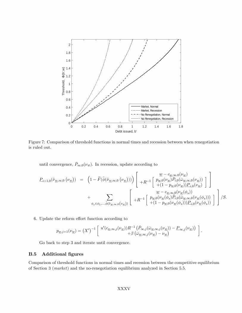
Debt issued, b'0 0.2 0.4 0.6 0.8 1 1.2 1.4 1.6 1.8

Thre

shol

d,(b

',w)

0

0.2

0.4

0.6

0.8

1

1.2

1.4

1.6

1.8

2

Market, NormalMarket, RecessionNo Renegotiation, NormalNo Renegotiation, Recession

Figure 7: Comparison of threshold functions in normal times and recession between when renegotiationis ruled out.

until convergence, �P1;0(� �w). In recession, update according to

P i+1;0(~�w;1;0��w�) =

�1� eF (~�(~�w;1;0 ��w�))�

24 w � cw;1;0(�w)

+R�1�pw;0(�w) �Pi;0(�!w;1;0(�w))+(1� pw;0(�w))P i;0(�w)

� 35+

X�s2�1;:::;~�(~�w;1;0(�w))

24 w � cw;1;0(�w(�s))

+R�1�pw;0(�w(�s) �Pi;0(�!w;1;0(�w(�s)))+(1� pw;0(�w(�s)))P i;0(�w(�s))

� 35 =S:

6. Update the reform e¤ort function according to

pw;j+1(�w) =�X 0��1 � u0(cw;1;j(�w))R�1 � �P1;j(�!w;1;j(�w))� P1;j(�w)�

+���!w;1;j(�w)� �w

� �:

Go back to step 3 and iterate until convergence.

B.5 Additional �gures

Comparison of threshold functions in normal times and recession between the competitive equilibriumof Section 3 (market) and the no-renegotiation equilibrium analyzed in Section 5.5.

XXXV