source reconstruction for spectrally-resolved bioluminescence ... · source reconstruction for...

Source Reconstruction forSpectrally-resolved Bioluminescence

Tomography with Sparse A prioriInformation

Yujie Lu1, Xiaoqun Zhang2, Ali Douraghy1, David Stout1, Jie Tian3,Tony F. Chan2, and Arion F. Chatziioannou1

1 David Geffen School of Medicine at UCLA, Crump Institute for Molecular Imaging,University of California, 570 Westwood Plaza, Los Angeles, CA 90095, USA

2 Department of Mathematics, University of California, Los Angeles, CA 900953 Medical Image Processing Group, Institute of Automation, Chinese Academy of Sciences,

P. O. Box 2728, Beijing, 100190, China

[email protected], [email protected]

Abstract: Through restoration of the light source information in smallanimals in vivo, optical molecular imaging, such as fluorescence moleculartomography (FMT) and bioluminescence tomography (BLT), can depictbiological and physiological changes observed using molecular probes. Apriori information plays an indispensable role in tomographic reconstruc-tion. As a type of a priori information, the sparsity characteristic of thelight source has not been sufficiently considered to date. In this paper, weintroduce a compressed sensing method to develop a new tomographicalgorithm for spectrally-resolved bioluminescence tomography. Thismethod uses the nature of the source sparsity to improve the reconstructionquality with a regularization implementation. Based on verification of theinverse crime, the proposed algorithm is validated with Monte Carlo-basedsynthetic data and the popular Tikhonov regularization method. Testing withdifferent noise levels and single/multiple source settings at different depthsdemonstrates the improved performance of this algorithm. Experimentalreconstruction with a mouse-shaped phantom further shows the potential ofthe proposed algorithm.

© 2009 Optical Society of America

OCIS codes: (110.6960) Tomography; (170.3010) Image reconstruction techniques;(170.6280) Spectroscopy, fluorescence and luminescence.

References and links1. R. Weissleder and U. Mahmood, “Molecular imaing,” Radiology 219, 316-333 (2001).2. V. Ntziachristos, J. Ripoll, L. V. Wang, and R. Weisslder, “Looking and listening to light: the evolution of whole

body photonic imaging,” Nat. Biotechnol. 23, 313-320 (2005).3. J. K. Willmann, N. van Bruggen, L. M. Dinkelborg, and S. S. Gambhir, “Molecular imaging in drug develop-

ment,” Nat. Rev. Drug Discovery 7, 591-607 (2008).4. C. H. Contag and M. H. Bachmann, “Advances in bioluminescence imaging of gene expression,” Annu. Rev.

Biomed. Eng. 4, 235-260 (2002).5. S. Bhaumik and S. S. Gambhir, “Optical imaging of renilla luciferase reporter gene expression in living mice,”

Proc. Natl. Acad. Sci. USA 99, 377-382 (2002).6. T. F. Massoud and S. S. Gambhir, “Molecular imaging in living subjects: seeing fundamental biological processes

in a new light,” Genes Dev. 17, 545-580 (2003).

(C) 2009 OSA 11 May 2009 / Vol. 17, No. 10 / OPTICS EXPRESS 8062#109156 - $15.00 USD Received 26 Mar 2009; revised 25 Apr 2009; accepted 26 Apr 2009; published 29 Apr 2009

7. G. Wang, E. A. Hoffman, G. McLennan, L. V. Wang, M. Suter, and J. F. Meinel, “Development of the firstbioluminescence CT scanner,” Radiology 566, 229 (2003).

8. G. Wang, Y. Li, and M. Jiang, “Uniqueness theorems in bioluminescence tomography,” Med. Phys. 31, 2289-2299 (2004).

9. G. Alexandrakis, F. R. Rannou, and A. F. Chatziioannou, “Tomographic bioluminescence imaging by use of acombined optical-PET (OPET) system: a computer simulation feasibility study,” Phys. Med. Biol. 50, 4225-4241(2005).

10. Y. Lv, J. Tian, W. Cong, and G. Wang, “Experimental study on bioluminescence tomography with multimodalityfusion,” Int. J. Biomed. Img. 1, 86741 (2007).

11. C. Kuo, O. Coquoz, D. G. Stearns, and B. W. Rice, “Diffuse luminescence imaging tomography of in vivobioluminescent markers using multi-spetral data,” in Proceedings of the 3rd International Meeting of the Society(MIT Press, 2004), p. 227.

12. A. J. Chaudhari, F. Darvas, J. R. Bading, R. A. Moats, P. S. Conti, D. J. Smith, S. R. Cherry, and R. M. Leahy,“Hyperspectral and multispectral bioluminescence optical tomography for small animal imaging,” Phys. Med.Biol. 50, 5421-5441 (2005).

13. H. Dehghani, S. C. Davis, S. Jiang, B. W. Pogue, K. D. Paulsen, and M. S. Patterson,“Spectrally resolved bioluminescence optical tomography,” Opt. Lett. 31, 365-367 (2006),http://www.opticsinfobase.org/abstract.cfm?URI=ol-31-3-365.

14. W. Cong, G. Wang, D. Kumar, Y. Liu, M. Jiang, L. V. Wang, E. A. Hoffman, G. McLennan, P. B. McCray,J. Zabner, and A. Cong, “Practical reconstruction method for bioluminescence tomography,” Opt. Express 13,6756-6771 (2005), http://www.opticsinfobase.org/oe/abstract.cfm?URI=oe-13-18-6756.

15. G. Wang, H. Shen, W. Cong, S. Zhao, and G. Wei, “Temperature-modulated bioluminescence tomography,” Opt.Express 14, 7852-7871 (2006), http://www.opticsinfobase.org/abstract.cfm?URI=oe-14-17-7852.

16. A. D. Klose, V. Ntziachristos, and A. H. Hielscher, “The inverse source problem based on the radiative transferequation in optical molecular imaging,” J. Comput. Phys. 202, 323-345 (2005).

17. A. P. Gibson, J. C. Hebden, and S. R. Arridge, “Recent advances in diffuse optical imaging,” Phys. Med. Biol.50, R1-R43 (2005).

18. Y. Lv, J. Tian, W. Cong, G. Wang, J. Luo, W. Yang, and H. Li, “A multilevel adaptivefinite element algorithm for bioluminescence tomography,” Opt. Express 14, 8211-8223 (2006),http://www.opticsinfobase.org/abstract.cfm?URI=oe-14-18-8211.

19. Y. Lv, J. Tian, W. Cong, G. Wang, W. Yang, C. Qin, and M. Xu, “Spectrally resolved bioluminescence tomogra-phy with adaptive finite element analysis: methodology and simulation,” Phys. Med. Biol. 52, 4497-4512 (2007).

20. X. Gu, Q. Zhang, L. Larcom, and H. Jiang, “Three-dimensional bioluminescence to-mography with model-based reconstruction,” Opt. Express 12, 3996-4000 (2004),http://www.opticsinfobase.org/oe/abstract.cfm?URI=oe-12-17-3996.

21. S. Holder, Electrical Impedance Tomography, (Institute of Physics Publishing, Bristol and Philadelphia, 2005).22. C. Kuo, O. Coquoz, T. L. Troy, H. Xu, and B. W. Rice, “Three-dimensional reconstruction of in vivo biolumines-

cent sources based on multispectral imaging,” J. Biomed. Opt. 12, 024007 (2007).23. W. Cong, K. Durairaj, L. V. Wang, and G. Wang, “A Born-type approximation method for bioluminescence

tomography,” Med. Phys. 33, 679-686 (2006).24. D. Donoho and I. Johnstone, “Ideal spatial adaption via wavelet shrinkage,” Biometrika 81, 425-455 (1994).25. S. G. Mallat and Z. Zhang, “Matching pursuits with time-frequency dictionaries,” IEEE Trans. Signal Process.

41, 3397-3415 (2002).26. L. Rudin, S. Osher, and E. Fatemi, “Nonlinear total variation based noise removal algorithms,” J. Phys. D 60,

259-268 (1992).27. E. J. Candes, J. K. Romberg, and T. Tao, “Stable signal recovery from incomplete and inaccurate measurements,”

Commun. Pur. Appl. Math. 59, 1207-1223 (2006).28. E. J. Candes, “Compressive sampling,” in Proceedings of the International Congress of Mathematicians, Madrid,

Spain 3, 1433-1452 (2006).29. C. Kuo, O. Coquoz, T. Troy, D. Zwarg, and B. Rice, “Bioluminescent tomography for in vivo localization and

quantification of luminescent sources from a multiple-view imaging system,” Mol. Img. 4, 370 (2005).30. G. Wang, H. Shen, K. Durairaj, X. Qian, and W. Cong, “The first bioluminescence tomography system for

simultaneous acquisition of multiview and multispectral data,” Int. J. Biomed. Img. 2006:Article ID 58601,(2006).

31. M. Schweiger, S. R. Arridge, M. Hiraoka, and D. T. Delpy, “The finite element method for the propagation oflight in scattering media: Boundary and source conditions,” Med. Phys. 22, 1779- 1792 (1995).

32. S. S. Rao, The finite element method in engineering, (Butterworth-Heinemann, Boston, 1999).33. R. Roy and E. M. Sevick-Muraca, “Active constrained truncated newton method

for simple-bound optical tomography,” J. Opt. Soc. Am. A 17, 1627-1641 (2000),http://www.opticsinfobase.org/abstract.cfm?URI=josaa-17-9-1627.

34. S. J. Benson and J. More, “A limited-memory variable-metric algorithm for bound-constrained minimization,”Technical Report ANL/MCS-P909-0901, Mathematics and Computer Science Division, Argonne National Lab-


oratory (2001).35. H. Li, J. Tian, F. Zhu, W. Cong, L. V. Wang, E. A. Hoffman, and G. Wang, “A mouse optical simulation envi-

roment (MOSE) to investigate bioluminescent phenomena in the living mouse with the Monte Carlo Method,”Acad. Radiol. 11, 1029-1038 (2004).

36. S. A. Prahl, M. J. C. van Gemert, and A. J. Welch, “Determining the optical proper-ties of turbid mediaby using the addingdoubling method,” Appl. Opt. 32, 559-568 (1993),http://www.opticsinfobase.org/abstract.cfm?URI=ao-32-4-559.

37. Michael Lustig, Sparse MRI, PhD thesis, Stanford University, 2008.38. D. Donoho, “For most large underdetermined systems of linear equations the minimal 1-norm solution is also

the sparsest solution,” Commun. Pur. Appl. Math. 59, 797-829 (2006).39. A. D. Klose and B. Beattie, “Bioluminescence tomography with SP3 equations,” in Biomedical Optics Topical

Meeting, 2008, http://www.opticsinfobase.org/abstract.cfm?URI=BIOMED-2008-BMC8.40. J. Cai, S. Osher and Z. Shen, “Convergence of the Linearized Bregman Iteration for �1-Norm Minimization,”

CAM report 08-52, 2008.

1. Introduction

In vivo small animal optical imaging has become an important tool of biological discoveryand preclinical applications [1][2][3]. When mouse models are labeled using optical molec-ular probes, the probes acting as light sources, reflect corresponding biological informationthrough the emission of visible or near infrared (NIR) light photons. Optical molecular imag-ing equipment is used to detect the photon distribution over the surface of the small animal tonon-invasively investigate these models [4]. In recent years, planar optical molecular imaging,and more specifically bioluminescence imaging, has been extensively applied in tumorigenesisstudies, cancer diagnosis, metastasis detection, drug discovery and development, and gene ther-apies given its convenience and ease operation [5][6]. The technology that is capable to acquirethree dimensional information of the light sources will become a next generation instrument foroptical molecular imaging. Bioluminescence tomography (BLT) is one such instrument beingdeveloped for this purpose [7].

An indispensable parameter for bioluminescence tomography is a priori information, whichcan be used to localize the optical sources. Theoretically, the source uniqueness proof givesus an important reference [8]. Practically, the richer the a priori information we apply, thefurther improvements BLT reconstruction can yield. Currently, three types of a priori informa-tion are verified and extensively applied in reconstruction algorithms. These include anatomi-cal information [9][10], spectrally-resolved measurements [11][12][9][13], and the distributionof surface photons [14]. Anatomical information is used to assign relevant optical propertiesto organs. Spectrally resolved data considers the source spectrum and the tissue absorptionand scattering characteristics. The use of these a priori information significantly improvessource reconstruction. The temperature dependent source spectral shift has recently led to atemperature-modulated bioluminescence tomography method which uses a focused ultrasoundarray [15]. In principle, this should belong to spectrally-resolved a priori information. The apriori permissible source region is defined by the surface photon distribution and improves thereconstruction by constraining the permissible source position [14]. Overall, it is necessary todefine additional a priori parameters for BLT reconstruction.

The diffusion approximation is extensively used in BLT reconstruction despite the fact thathigher approximations of the radiative transfer equation lead to improved reconstructed resultsin some situations [16]. The finite element method (FEM), analytical formulations and Bornapproximation theory have been applied in combination with the diffusion equation [17]. TheFEM has become popular due to its ability to process complex heterogeneous geometries. Theadaptive strategy has also been developed to further improve the reconstruction based on theFEM [18][19]. In BLT, although nonlinear optimization strategies [20] used in diffuse opticaltomography (DOT) and expectation maximization (EM) algorithms [9] similar with that in


positron emission tomography (PET) are used, a linear least square (LS) problem is easilyobtained because of the linear nature of the BLT problem [14]. Meanwhile, the inverse crimeneeds to be carefully considered especially when new algorithms are evaluated using syntheticdata [21].

BLT reconstruction is an ill-posed problem. Inhibiting noise in measured data and reducingthe ill-posedness is necessary to obtain BLT reconstructions. Regularization is a useful methodfor such problems. Currently, the weighted least square method is used to reduce the measurednoise effects [22][14]. The Tikhonov regularization is a popular method and is extensively ap-plied in BLT reconstruction [23][19]. Mathematically, the Tikhonov method is aiming to stabi-lize the inverse of an ill-conditioned operator by minimizing a trade-off between a loss functionand the l2-norm of the signals. The advantage of the l2 norm is that the associated optimizationproblem can be efficiently solved using a classic quadratic minimization algorithm. The disad-vantage is that the solution obtained is often smoothed everywhere, resulting the loss of highfrequency structures of the original signal, especially in the case of noise. Over the past severalyears, the l1 norm regularization has been investigated in the signal and image processing fields,such as wavelet thresholding denoising [24], basis pursuit [25], and total variation for edge pre-serving reconstruction [26]. Moreover, a new sampling theory related to l1 minimization, knownas compressed sensing (or compressed sampling) provides a strong theoretical foundation forsparse approximations [27][28]. More accurately, this theory allows an exact reconstructionfrom a greatly reduced number of measurements through the use of convex programming. Inother words, if the real signals or images are sparse on some basis and the measurement operatorand sparsity basis satisfy certain coherent conditions, then the original sparse signal can be re-constructed with a greatly reduced sampling rate. In BLT, the unknown sources are contained inthe reconstructed domain (such as a mouse). Non-invasive measurements only acquire the sur-face distribution of photons emitted by bioluminescence sources. When using small elements(such as tetrahedron or hexahedron) to discretize the whole domain, the number of the surfacediscretized points is significantly fewer than that of the volumetric discretized points. The un-dersampling is inevitable for BLT reconstruction. Compared with single view measurements,multi-view data acquisition improves the BLT reconstruction to a certain degree [29][30], butit limits the high throughput ability of optical imaging. Single view measurements need to befurther investigated for improved BLT reconstruction.

Fortunately, when we use optical probes to observe the specified biological process of in-terest, the domain of the light source is relatively small and sparse compared with the entirereconstruction domain, in this case the mouse body. Here, by a combination of this a prioriinformation and compressed sensing theory, a novel spectrally-resolved bioluminescence re-construction algorithm is proposed. Specifically, based on the diffusion approximation model,the linear relationship between the spectrally-resolved measured data and the unknown sourcedistribution is established by using the FEM. The l1 norm as a regularization term is combinedinto the BLT least squares problem, realizing the compressed sensing method. In order to re-duce memory and time cost, a limited memory variable metric optimization method is usedto solve the bound-constrained BLT problem. In numerical verifications, the inverse crime isdemonstrated for different synthetic data sets from different finite element meshes and differentsimulation methods, showing that the Monte Carlo method is necessary for accurate simulationtests. Furthermore, BLT reconstructions with different noise levels and different source depthsdemonstrate the usefulness of the compressing sensing method-based l1 norm regularization,especially for sources located deep within tissues and having high noise. Finally, the proposedalgorithm is further tested by experimental reconstruction. In the next section, we present thespectrally-resolved BLT framework based on l1 regularization. In the third section, we evaluatethe performance of the proposed algorithm with various source settings. In the final section,


we discuss the relevant issues and conclusions. To the best of the authors knowledge, this con-tribution represents the first time that bioluminescence source sparse characteristic is used toimprove BLT reconstruction with the compressed sensing method.

2. Model

2.1. Photon diffusion model

The available bioluminescence probes typically emit photons in the range of 400-800nm. Thediffusion models as the P1 approximation to the radiative transfer equation have been ex-tensively applied in bioluminescence imaging. As the optical properties of biological tissueschange depending on the wavelength, the diffusion model is also a function of the wave-length. Assuming the bioluminescence source intensity is stable when photons are collected,the steady-state diffusion equation can be used to depict the photon propagation in tissues:

−∇·(D(r,λ )∇Φ(r,λ ))+ μa(r,λ )Φ(r,λ ) = S(r,λ ) (r ∈ Ω) (1)

where Ω and λ is the domain and the wavelength respectively; Φ(r,λ ) denotes the pho-ton flux density; S(r,λ ) is the source energy density; μa(r,λ ) is the absorption coefficient;D(r,λ )=1/(3(μa(r,λ )+(1−g)μs(r,λ ))) is the optical diffusion coefficient, μs(r,λ ) the scat-tering coefficient, and g is the anisotropy parameter. On the boundary ∂Ω, the Robin boundarycondition is used to depict the refractive index mismatch between the external medium n′ andΩ:

Φ(r,λ )+2A(r;n,n′)D(r,λ )(v(r)·∇Φ(r,λ )

)=0 (r ∈ ∂Ω) (2)

where v is the unit outer normal on ∂Ω. A(r;n,n′) can be approximately represented as:

A(r;n,n′) ≈ 1+R(r)1−R(r)

(3)

where n′ is close to 1.0 when the mouse is in air; R(r) can be approximated by R(r) ≈−1.4399n−2 + 0.7099n−1 + 0.6681 + 0.0636n [31]. When practical measurements are per-formed with a set of bandpass filters, the measured quantity is the outgoing flux density Q(r,λ )on the discretized wavelength λi, which is:

Q(r,λi) = −D(r,λi)(v·∇Φ(r,λi)

)=

Φ(r,λi)2A(r;n,n′)

(r ∈ ∂Ω) (4)

2.2. Linear Relationship Establishment

Based on the finite element theory [32], the weak solution of the flux density Φ(r,λi)∈H1(Ω)is given considering Eqs. (1) and (2) for a specified wavelength λi:

∫

Ω

(D(r,λi)

(∇Φ(r,λi)

)·(∇Ψ(r))+ μa(r,λi)Φ(r,λi)Ψ(r)

)dr

+∫

∂Ω

12An(r)

Φ(r,λi)Ψ(r)dr =∫

ΩS(r,λi)Ψ(r)dr (5)

where ∀Ψ(r)∈H1(Ω), H1(Ω) is the Sobolev space, and Ψ(r) is an arbitrary piece-wise testfunction. In the numerical finite element computation, the domain Ω needs to be discretizedinto a group of small elements τ . Correspondingly in three dimensional computations, Ψ(r)is disretized as shape functions regarding the element τ . Tetrahedra and hexahedra are usuallyused as τ . Regardless of the specified element and shape function, we get the following finiteelement-based matrix form when the source term is unknown:

(K(λi)+C(λi)+B(λi)

)Φ(λi)=F(λi)S(λi) (6)


where λi, K(λi), C(λi) and B(λi) are called the mass, stiff and boundary matrix respectively.These are obtained from the first, second and third term in Eq. 5’s right side [14]. Note thatF(λi) can be flexibly selected depending on the choice of S(λi). Generally, we may selectdiscretized elements or points as the unknown variables. Here, we use the point-based mode.When K(λi), C(λi) and B(λi) are summed as M(λi), we have:

Φb(λi) = F (λi)S(λi) (7)

Here, we consider the linear relationship between the unknown source variable S(λi) and theflux density Φb(λi) at the measurable boundary discretized points. F (λi) can be adjustablyobtained regarding the whole domain, or a priori or a posteriori permissible source region asunknown source region [19]. When the energy percentage of the wavelength λi is γi, we get:

Φb = A S (8)

where

Φb =

⎡

⎢⎢⎢⎢⎢⎢⎣

Φb(λ1)...

Φb(λi)...

Φb(λI)

⎤

⎥⎥⎥⎥⎥⎥⎦

, A =

⎡

⎢⎢⎢⎢⎢⎢⎣

γ1F (λ1)...

γiF (λi)...

γIF (λI)

⎤

⎥⎥⎥⎥⎥⎥⎦

(9)

Total energy S at all the wavelengths will be ∑Ii=1 γiS(λi), where I is the total wavelength num-

ber.

2.3. Regularization

In optical tomographic imaging, the physical meaning of the various parameters and constrain-ing minimization problem by optimization methods have significant impact on object recon-struction [33]. Therefore, for Eq. 8, we get the following constrained minimization problem forthe measured signal Φmeas which corresponds to Φb:

minS

12‖A S−Φmeas‖2 s. t. D = {0 ≤ S ≤ Ssup} (10)

where Ssup is a known upper bound vector and ‖ · ‖ denotes l2 norm of a vector. If we ignorethe constraints, this also corresponds to solving the normal equation

A T A S=A T Φmeas

When the spectrum of the operator A T A is unbounded or ill-conditioned, the inverse of thisequation can cause severe numerical instabilities. A standard procedure is to integrate a prioriinformation in the solution, called regularization. For example, the simplest Tikhonov regular-ization consists of adding a l2 norm penalty term to the l2 loss functional, i. e.

minS

12‖A S−Φmeas‖2 +

δ2‖S‖2 s. t. D = {0 ≤ S ≤ Ssup}. (11)

where δ is a positive number called the regularization parameter which is used to balance thefidelity term and the regularization term. The related gradient of the objective function of Eq.11 is written as:

∇Θ(S) = A T (A S−Φmeas)+δS.


This quadratic functional can be efficiently solved by a large range of convex programmingtechnique.

However, this quadratic stabilizer intends to recover a smoothed version of S independentof the data structure. It is often incapable of recovering local singularities or discontinuitiespresented in the object in the case of noise. We are now considering a non-quadratic lp normpenalty where 1 ≤ p < 2, since the functional ceases to be convex if p < 1. The main advantageof the non quadratic norm is to promote the sparsity of the solution. Roughly speaking, whenp → 1, large components of S are less penalized when compared to the quadratic norm. How-ever, the sum of small components are more penalized, thus leading to a sparse solution. In BLT,an important a priori information is the sparsity of the light source, therefore l1 regularizationis a more natural choice for this ill posed inverse problem. It follows the model:

minS

Θ(S) :12‖A S−Φmeas‖2 +

δ2‖S‖1 s. t. D = {0 ≤ S ≤ Ssup} (12)

where ‖S‖1 = ∑i |Si| denotes the l1 of the vector S. Since this functional is non-differentiable,we can use a differentiable approximation defined as ‖S‖1 ≈ ∑n

i=1 Fε(S(i)) [40] defined as

Fε(ξ ) =

{|ξ |− ε

2 , if |ξ | > εξ 2

2ε , if |ξ | ≤ ε.

where ε is a small positive number.

2.4. Algorithm

Algorithm 1 Regularization-based BLMVM algorithm for BLT reconstruction

Require: Choose S0 ∈ D . Let d0 = −TD∇Θ(S0).

1: for k = 0 to kmax do2: Compute αk using a projected line search.3: Compute Sk+1 using P[Sk +αkdk].4: Compute ∇Θ(Sk+1) and its projection TD∇Θ(Sk+1).5: if ‖TD∇Θ(Sk+1) < ε‖ then6: Stop.7: else8: Compute sk and yk using Sk+1 −Sk and TD∇Θ(Sk+1)−TD∇Θ(Sk) respectively.9: if yT

k sk > 0 then10: Update Hk by Eq. 15.11: end if12: Compute Hk+1∇Θ(Sk+1) using the L-BFGS two-loop recursion.13: if 〈−TD(Hk+1∇Θ(Sk+1)),∇Θ(Sk+1)〉 > 0 then14: d = −Hk+1∇Θ(Sk+1).15: else16: d = −∇Θ(Sk+1).17: end if18: end if19: end for

Through minimizing the objective function Θ(S), BLT reconstruction can be obtained. Θ(S) isa typical bound-constrained regularization-based least square problem. For the constraint prob-lem, an active-set strategy which includes several types of Hessian matrix based optimization


algorithms is adopted to obtain a desirable reconstruction [14][19]. Although this least squareproblem easily obtains the Hessian matrix, it requires a significant amount of memory duringthe optimization procedure, especially for large-scale problems. In addition, when computingthe search direction, it is necessary to invert the Hessian matrix, which is time-consuming andseverely affects the speed of BLT reconstruction. One solution is to use quasi-Newton methods.Generally, these build up an approximate Hessian matrix by using gradients and iteration algo-rithms. This approximate matrix is obtained in real-time by vector-vector multiplications and iseasy to invert, saving memory and time requirements. Here, the limited memory variable metricbound constrained quasi-Newton method (BLMVM) [34] is used for BLT reconstruction. Thedetailed algorithm is shown in Algorithm 1.

Specifically, an initial guess S0 for the source distribution should be given and the initialsearching direction d0 is also provided. Here, the operator TD is defined as

[TDd]( j) =

⎧⎨

⎩

d( j) if S( j) ∈ (0,S( j)sup)min{d( j),0} if S( j) = 0max{d( j),0} if S( j) = S( j)sup

(13)

where d( j),S( j) denotes the j-th element of d and S respectively. When the step size αk isdetermined, the iterative solution at the next step Sk+1 can be calculated through the projectionoperator P onto the box constraint, defined as

[PDS]( j) =

⎧⎨

⎩

S( j) if S( j) ∈ [0,S( j)sup]0 if S( j) ≤ 0S( j)sup if S( j) > S( j)sup

(14)

During the minimization procedure, the approximation Hk+1 of the inverse Hessian matrix atthe next step is updated when yT

k sk > 0

Hk+1 = V Tk HkVk +ρks

Tk sk (15)

where ρk = 1/(yTk sk),Vk = I − ρk(yksT

k ), I is the identity matrix. Since the inverse Hessianmatrix is usually dense, the memory and time requirements for processing Hk is prohibitiveespecially for large scale problems. In the BLMVM algorithm, a limited memory BFGS ma-trix is obtained by the vector pairs from the last m iterations. Given an initial inverse Hessianapproximation H0

k+1, the updated matrix Hk is obtained

Hk = ( V Tk−1 · · ·V T

k−m)H0k (Vk−m · · ·Vk−1)

+ ρk−m(V Tk−1 · · ·V T

k−m+1)sk−msTk−m(Vk−m+1 · · ·Vk−1)

... (16)

+ ρk−2(Vk−1)T sk−2sTk−1(Vk−1)

+ ρk−1sk−1sTk−1

3. Results

3.1. Simulation verifications

Much attention should always be given to the inverse crime when new algorithms are verifiedusing synthetic data. Monte Carlo methods can simulate the photon propagation better giventhe ability to incorporate Poisson noise in the simulation. In addition, the same discretizedmodes used in the forward simulation and inverse reconstruction will significantly affect the


evaluation. A cubic domain with a width of 15mm was used to confirm these effects. The syn-thetic data was obtained through three types of modes, which are hexahedra- and tetrahedra-based FEM, and Monte Carlo method. The diffusion approximation equation was used in theFEM-based simulation. The same discretization with hexahedra-based simulation was used inBLT reconstruction and its element size was 1.0mm in width. The average element diameterin tetrahedra-based discretization was also 1.0mm. Figures 1(a) and 1(b) show the discretizedmeshes. In reconstruction, three wavelengths (600nm, 650nm and 700nm) were used to obtainspectrally-resolved measurements. We refer to the literature [9] to obtain the correspondingoptical properties as listed in Table 1. Photon attenuation is approximately an exponential func-tion of the effective attenuation coefficient μe f f (μe f f =

√3μa(μ ′

s + μa)). In order to preservethe noise effect for all the wavelengths, we sampled 107 photons for 600nm and half the num-ber of these photons were used at two other wavelengths. Monte Carlo simulation is severelytime-consuming. To accelerate the simulation, MPI-based parallel code based on the MolecularOptical Simulation Environment (MOSE) [35] was developed in order to perform spectrally-resolved simulations. Because the parallel program only records the information of the photonsemitted through the boundary, we can consider that the cubic domain used in the MC methodis not discretized, as shown in Fig. 1(c).

Table 1. Optical property at three wavelengths for cubic phantom in simulation verifications

Wavelength 600nm 650nm 700nmμa(λi)[mm−1] 0.19 0.038 0.022μ ′

s(λi)[mm−1] 1.66 1.53 1.41

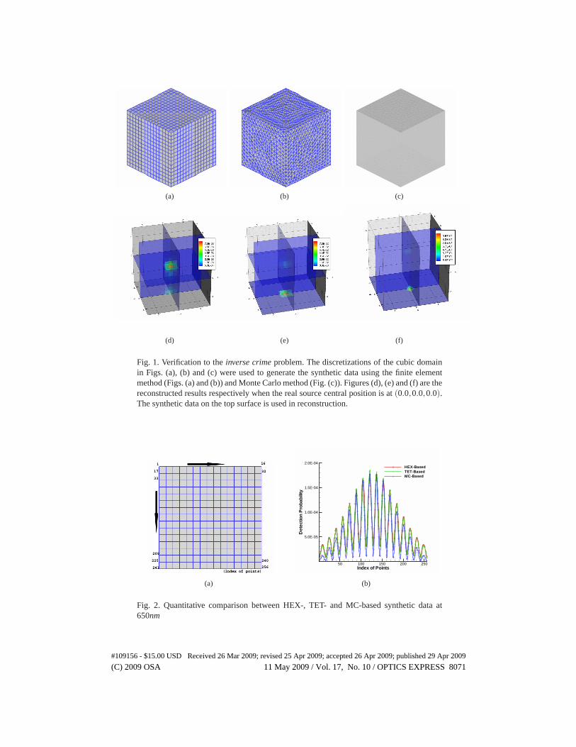
When generating the synthetic data, a cubic source with a width of 1mm was placed at thecenter of the cubic domain. The source intensity at every wavelength was set to “1.0”. In thereconstruction, we used the synthetic data on the top surface, while the additional noise was notconsidered. Additionly, regularization methods were not used. Based on three different typesof synthetic data, the reconstructed results are shown in Figs. 1(d) to 1(f). When using the hex-ahedral mesh, the same mathematical model and discretized mesh were used in synthetic datageneration and reconstruction. Although there are some artifacts in the reconstructed results,the source position is well localized, as seen in Fig. 1(d). However, when the tetrahedral-basedsynthetic data is used, the reconstructed results become inaccurate. Also, in Fig. 1(e), it is ob-served that there are some reconstructed results below the actual source position. MC-basedreconstructed results in Fig. 1(f) are similar with those based on the tetrahedral mesh. Thedifference is that the reconstruction around the actual source position becomes increasingly ob-scure and its position is proximal to the top surface. Actually, the use of different simulationmethods results in different levels of noise in the synthetic data, affecting the reconstructed re-sults. Therefore, the synthetic data results are compared in terms of the three different methodsand the results are shown in Fig. 2(b). We can find the Hex- and Tet-based synthetic data is al-most the same. The maximal relative error (RE) (RE = (ΦTet −ΦHex)/ΦHex) between them isonly 10.4%. However, these errors introduce significant effects during reconstruction, showingthe ill-posedness of the BLT problem and the necessity of regularization. Furthermore, we cansee there are large errors between the Hex- and MC-based data especially when the discretizedpoints are far from the center. It is clear that this produces the poor reconstructed results. Fromanother aspect, it is necessary to use the MC-based synthetic data for testing the proposed al-gorithm due to its precise simulation and the inverse crime problem. Note that for convenientcomparison the MC-based data is normalized using the Hex-based data based on its respectivemaximal flux density.


(a) (b) (c)

(d) (e) (f)

Fig. 1. Verification to the inverse crime problem. The discretizations of the cubic domainin Figs. (a), (b) and (c) were used to generate the synthetic data using the finite elementmethod (Figs. (a) and (b)) and Monte Carlo method (Fig. (c)). Figures (d), (e) and (f) are thereconstructed results respectively when the real source central position is at (0.0,0.0,0.0).The synthetic data on the top surface is used in reconstruction.

(a)

Index of Points

Det

ectio

nP

roba

bili

ty

50 100 150 200 250

5.0E-05

1.0E-04

1.5E-04

2.0E-04HEX-BasedTET-BasedMC-Based

(b)

Fig. 2. Quantitative comparison between HEX-, TET- and MC-based synthetic data at650nm


3.1.1. Single Source Cases with the Homogeneous Media

(a) (b) (c)

(d) (e) (f)

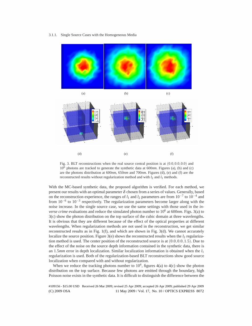
Fig. 3. BLT reconstructions when the real source central position is at (0.0,0.0,0.0) and106 photons are tracked to generate the synthetic data at 600nm. Figures (a), (b) and (c)are the photons distribution at 600nm, 650nm and 700nm. Figures (d), (e) and (f) are thereconstructed results without regularization method and with l2 and l1 methods.

With the MC-based synthetic data, the proposed algorithm is verified. For each method, wepresent our results with an optimal parameter δ chosen from a series of values. Generally, basedon the reconstruction experience, the ranges of l1 and l2 parameters are from 10−7 to 10−4 andfrom 10−6 to 10−3 respectively. The regularization parameters become larger along with thenoise increase. In the single source case, we use the same settings with those used in the in-verse crime evaluations and reduce the simulated photon number to 106 at 600nm. Figs. 3(a) to3(c) show the photon distribution on the top surface of the cubic domain at three wavelengths.It is obvious that they are different because of the effect of the optical properties at differentwavelengths. When regularization methods are not used in the reconstruction, we get similarreconstructed results as in Fig. 1(f), and which are shown in Fig. 3(d). We cannot accuratelylocalize the source position. Figure 3(e) shows the reconstructed results when the l2 regulariza-tion method is used. The center position of the reconstructed source is at (0.0,0.0,1.5). Due tothe effect of the noise on the source depth information contained in the synthetic data, there isan 1.5mm error in depth localization. Similar localization information is obtained when the l1regularization is used. Both of the regularization-based BLT reconstructions show good sourcelocalization when compared with and without regularization.

When we reduce the tracking photons number to 104, figures 4(a) to 4(c) show the photondistribution on the top surface. Because few photons are emitted through the boundary, highPoisson noise exists in the synthetic data. It is difficult to distinguish the difference between the


(a) (b) (c)

(d) (e) (f)

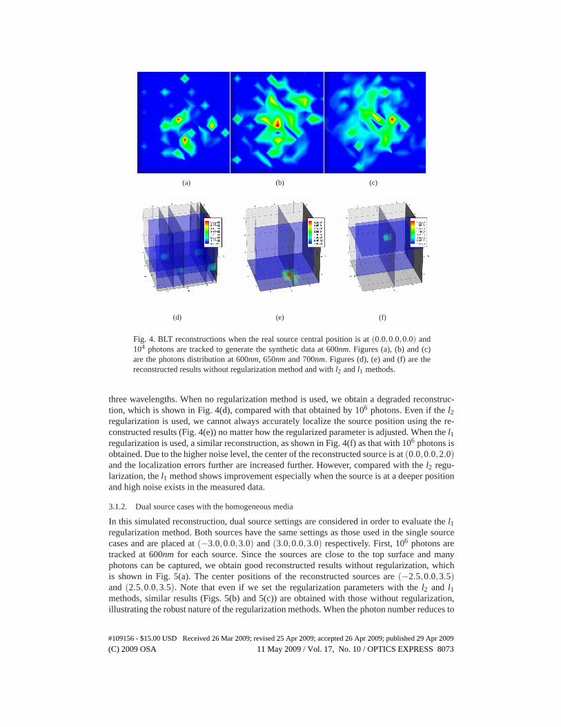
Fig. 4. BLT reconstructions when the real source central position is at (0.0,0.0,0.0) and104 photons are tracked to generate the synthetic data at 600nm. Figures (a), (b) and (c)are the photons distribution at 600nm, 650nm and 700nm. Figures (d), (e) and (f) are thereconstructed results without regularization method and with l2 and l1 methods.

three wavelengths. When no regularization method is used, we obtain a degraded reconstruc-tion, which is shown in Fig. 4(d), compared with that obtained by 106 photons. Even if the l2regularization is used, we cannot always accurately localize the source position using the re-constructed results (Fig. 4(e)) no matter how the regularized parameter is adjusted. When the l1regularization is used, a similar reconstruction, as shown in Fig. 4(f) as that with 106 photons isobtained. Due to the higher noise level, the center of the reconstructed source is at (0.0,0.0,2.0)and the localization errors further are increased further. However, compared with the l2 regu-larization, the l1 method shows improvement especially when the source is at a deeper positionand high noise exists in the measured data.

3.1.2. Dual source cases with the homogeneous media

In this simulated reconstruction, dual source settings are considered in order to evaluate the l1regularization method. Both sources have the same settings as those used in the single sourcecases and are placed at (−3.0,0.0,3.0) and (3.0,0.0,3.0) respectively. First, 106 photons aretracked at 600nm for each source. Since the sources are close to the top surface and manyphotons can be captured, we obtain good reconstructed results without regularization, whichis shown in Fig. 5(a). The center positions of the reconstructed sources are (−2.5,0.0,3.5)and (2.5,0.0,3.5). Note that even if we set the regularization parameters with the l2 and l1methods, similar results (Figs. 5(b) and 5(c)) are obtained with those without regularization,illustrating the robust nature of the regularization methods. When the photon number reduces to


(a) (b) (c)

(d) (e) (f)

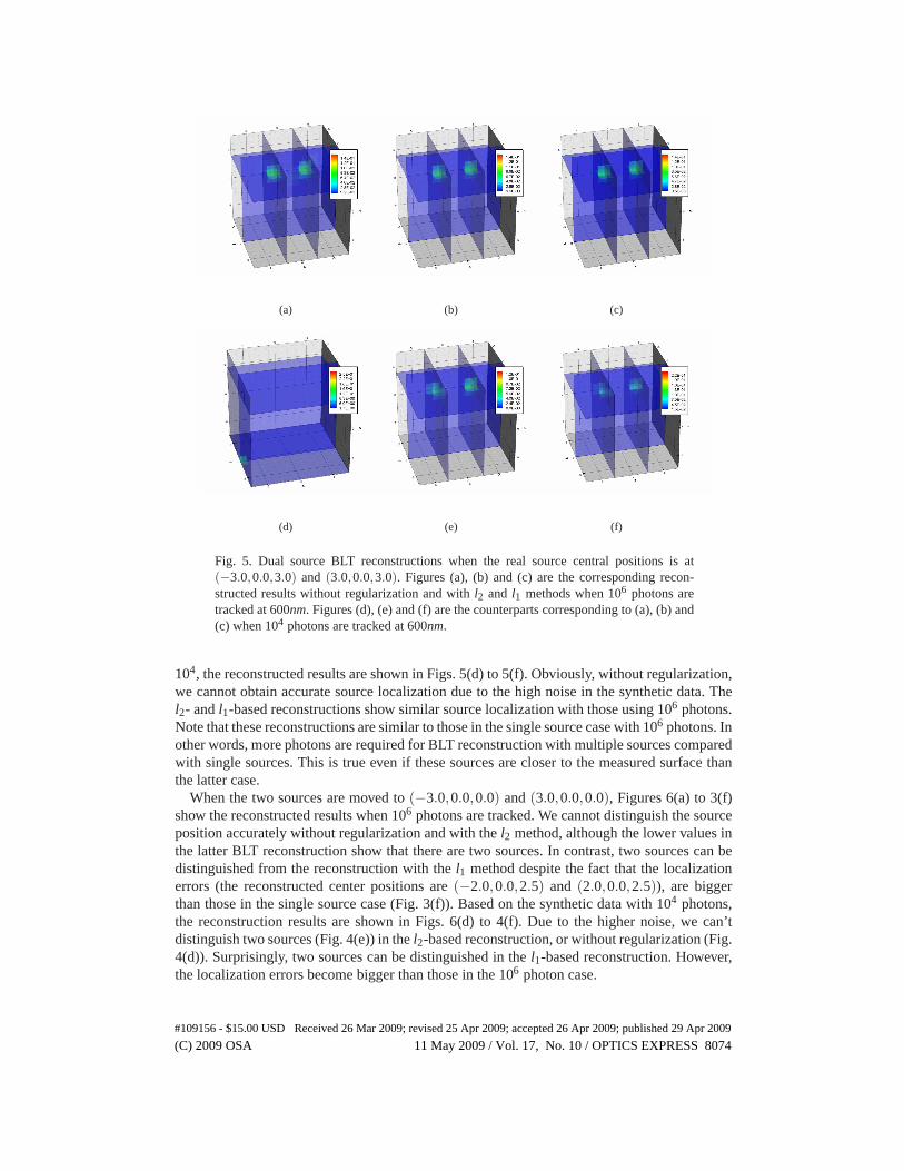
Fig. 5. Dual source BLT reconstructions when the real source central positions is at(−3.0,0.0,3.0) and (3.0,0.0,3.0). Figures (a), (b) and (c) are the corresponding recon-structed results without regularization and with l2 and l1 methods when 106 photons aretracked at 600nm. Figures (d), (e) and (f) are the counterparts corresponding to (a), (b) and(c) when 104 photons are tracked at 600nm.

104, the reconstructed results are shown in Figs. 5(d) to 5(f). Obviously, without regularization,we cannot obtain accurate source localization due to the high noise in the synthetic data. Thel2- and l1-based reconstructions show similar source localization with those using 106 photons.Note that these reconstructions are similar to those in the single source case with 106 photons. Inother words, more photons are required for BLT reconstruction with multiple sources comparedwith single sources. This is true even if these sources are closer to the measured surface thanthe latter case.

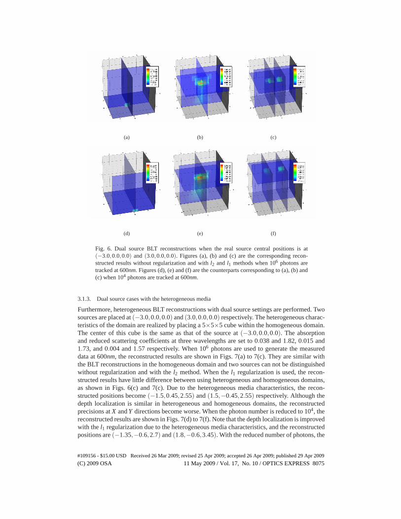
When the two sources are moved to (−3.0,0.0,0.0) and (3.0,0.0,0.0), Figures 6(a) to 3(f)show the reconstructed results when 106 photons are tracked. We cannot distinguish the sourceposition accurately without regularization and with the l2 method, although the lower values inthe latter BLT reconstruction show that there are two sources. In contrast, two sources can bedistinguished from the reconstruction with the l1 method despite the fact that the localizationerrors (the reconstructed center positions are (−2.0,0.0,2.5) and (2.0,0.0,2.5)), are biggerthan those in the single source case (Fig. 3(f)). Based on the synthetic data with 104 photons,the reconstruction results are shown in Figs. 6(d) to 4(f). Due to the higher noise, we can’tdistinguish two sources (Fig. 4(e)) in the l2-based reconstruction, or without regularization (Fig.4(d)). Surprisingly, two sources can be distinguished in the l1-based reconstruction. However,the localization errors become bigger than those in the 106 photon case.


(a) (b) (c)

(d) (e) (f)

Fig. 6. Dual source BLT reconstructions when the real source central positions is at(−3.0,0.0,0.0) and (3.0,0.0,0.0). Figures (a), (b) and (c) are the corresponding recon-structed results without regularization and with l2 and l1 methods when 106 photons aretracked at 600nm. Figures (d), (e) and (f) are the counterparts corresponding to (a), (b) and(c) when 104 photons are tracked at 600nm.

3.1.3. Dual source cases with the heterogeneous media

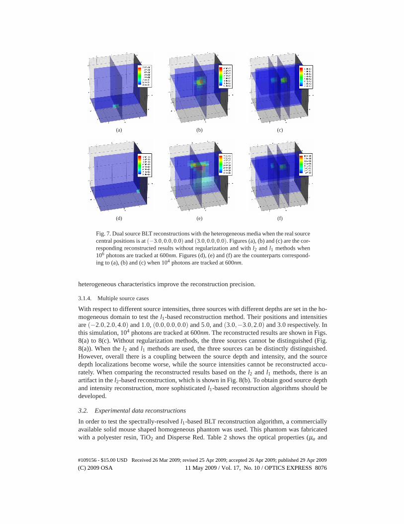
Furthermore, heterogeneous BLT reconstructions with dual source settings are performed. Twosources are placed at (−3.0,0.0,0.0) and (3.0,0.0,0.0) respectively. The heterogeneous charac-teristics of the domain are realized by placing a 5×5×5 cube within the homogeneous domain.The center of this cube is the same as that of the source at (−3.0,0.0,0.0). The absorptionand reduced scattering coefficients at three wavelengths are set to 0.038 and 1.82, 0.015 and1.73, and 0.004 and 1.57 respectively. When 106 photons are used to generate the measureddata at 600nm, the reconstructed results are shown in Figs. 7(a) to 7(c). They are similar withthe BLT reconstructions in the homogeneous domain and two sources can not be distinguishedwithout regularization and with the l2 method. When the l1 regularization is used, the recon-structed results have little difference between using heterogeneous and homogeneous domains,as shown in Figs. 6(c) and 7(c). Due to the heterogeneous media characteristics, the recon-structed positions become (−1.5,0.45,2.55) and (1.5,−0.45,2.55) respectively. Although thedepth localization is similar in heterogeneous and homogeneous domains, the reconstructedprecisions at X and Y directions become worse. When the photon number is reduced to 104, thereconstructed results are shown in Figs. 7(d) to 7(f). Note that the depth localization is improvedwith the l1 regularization due to the heterogeneous media characteristics, and the reconstructedpositions are (−1.35,−0.6,2.7) and (1.8,−0.6,3.45). With the reduced number of photons, the


(a) (b) (c)

(d) (e) (f)

Fig. 7. Dual source BLT reconstructions with the heterogeneous media when the real sourcecentral positions is at (−3.0,0.0,0.0) and (3.0,0.0,0.0). Figures (a), (b) and (c) are the cor-responding reconstructed results without regularization and with l2 and l1 methods when106 photons are tracked at 600nm. Figures (d), (e) and (f) are the counterparts correspond-ing to (a), (b) and (c) when 104 photons are tracked at 600nm.

heterogeneous characteristics improve the reconstruction precision.

3.1.4. Multiple source cases

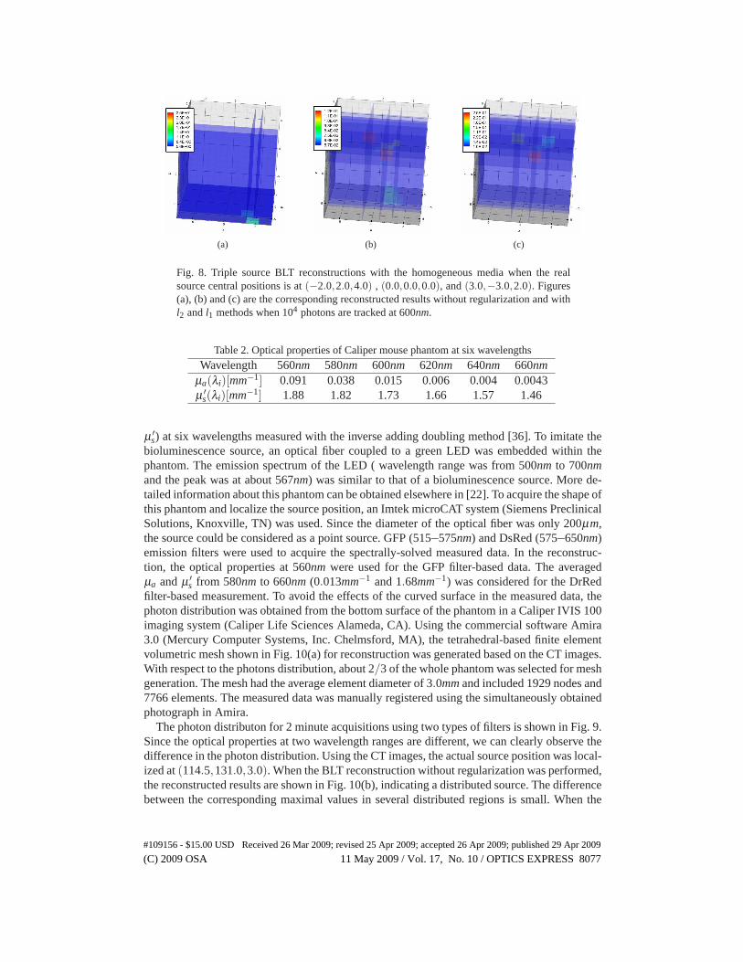
With respect to different source intensities, three sources with different depths are set in the ho-mogeneous domain to test the l1-based reconstruction method. Their positions and intensitiesare (−2.0,2.0,4.0) and 1.0, (0.0,0.0,0.0) and 5.0, and (3.0,−3.0,2.0) and 3.0 respectively. Inthis simulation, 104 photons are tracked at 600nm. The reconstructed results are shown in Figs.8(a) to 8(c). Without regularization methods, the three sources cannot be distinguished (Fig.8(a)). When the l2 and l1 methods are used, the three sources can be distinctly distinguished.However, overall there is a coupling between the source depth and intensity, and the sourcedepth localizations become worse, while the source intensities cannot be reconstructed accu-rately. When comparing the reconstructed results based on the l2 and l1 methods, there is anartifact in the l2-based reconstruction, which is shown in Fig. 8(b). To obtain good source depthand intensity reconstruction, more sophisticated l1-based reconstruction algorithms should bedeveloped.

3.2. Experimental data reconstructions

In order to test the spectrally-resolved l1-based BLT reconstruction algorithm, a commerciallyavailable solid mouse shaped homogeneous phantom was used. This phantom was fabricatedwith a polyester resin, TiO2 and Disperse Red. Table 2 shows the optical properties (μa and


(a) (b) (c)

Fig. 8. Triple source BLT reconstructions with the homogeneous media when the realsource central positions is at (−2.0,2.0,4.0) , (0.0,0.0,0.0), and (3.0,−3.0,2.0). Figures(a), (b) and (c) are the corresponding reconstructed results without regularization and withl2 and l1 methods when 104 photons are tracked at 600nm.

Table 2. Optical properties of Caliper mouse phantom at six wavelengths

Wavelength 560nm 580nm 600nm 620nm 640nm 660nmμa(λi)[mm−1] 0.091 0.038 0.015 0.006 0.004 0.0043μ ′

s(λi)[mm−1] 1.88 1.82 1.73 1.66 1.57 1.46

μ ′s) at six wavelengths measured with the inverse adding doubling method [36]. To imitate the

bioluminescence source, an optical fiber coupled to a green LED was embedded within thephantom. The emission spectrum of the LED ( wavelength range was from 500nm to 700nmand the peak was at about 567nm) was similar to that of a bioluminescence source. More de-tailed information about this phantom can be obtained elsewhere in [22]. To acquire the shape ofthis phantom and localize the source position, an Imtek microCAT system (Siemens PreclinicalSolutions, Knoxville, TN) was used. Since the diameter of the optical fiber was only 200μm,the source could be considered as a point source. GFP (515−575nm) and DsRed (575−650nm)emission filters were used to acquire the spectrally-solved measured data. In the reconstruc-tion, the optical properties at 560nm were used for the GFP filter-based data. The averagedμa and μ ′

s from 580nm to 660nm (0.013mm−1 and 1.68mm−1) was considered for the DrRedfilter-based measurement. To avoid the effects of the curved surface in the measured data, thephoton distribution was obtained from the bottom surface of the phantom in a Caliper IVIS 100imaging system (Caliper Life Sciences Alameda, CA). Using the commercial software Amira3.0 (Mercury Computer Systems, Inc. Chelmsford, MA), the tetrahedral-based finite elementvolumetric mesh shown in Fig. 10(a) for reconstruction was generated based on the CT images.With respect to the photons distribution, about 2/3 of the whole phantom was selected for meshgeneration. The mesh had the average element diameter of 3.0mm and included 1929 nodes and7766 elements. The measured data was manually registered using the simultaneously obtainedphotograph in Amira.

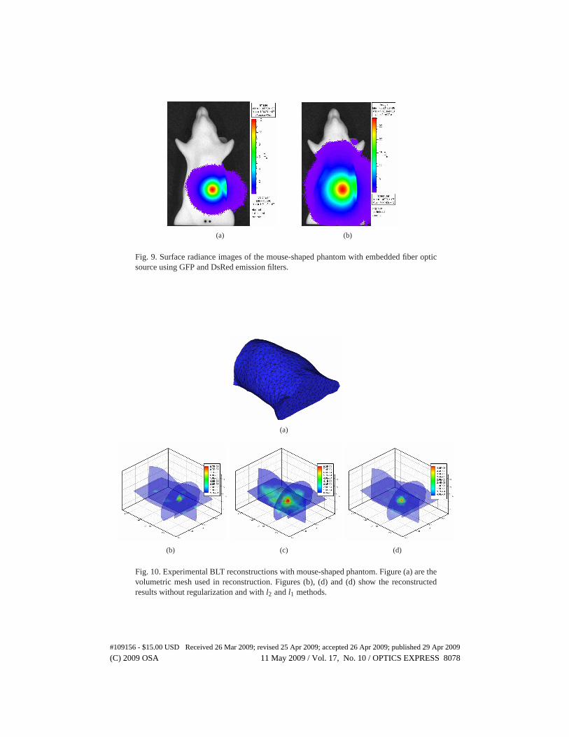
The photon distributon for 2 minute acquisitions using two types of filters is shown in Fig. 9.Since the optical properties at two wavelength ranges are different, we can clearly observe thedifference in the photon distribution. Using the CT images, the actual source position was local-ized at (114.5,131.0,3.0). When the BLT reconstruction without regularization was performed,the reconstructed results are shown in Fig. 10(b), indicating a distributed source. The differencebetween the corresponding maximal values in several distributed regions is small. When the


(a) (b)

Fig. 9. Surface radiance images of the mouse-shaped phantom with embedded fiber opticsource using GFP and DsRed emission filters.

(a)

(b) (c) (d)

Fig. 10. Experimental BLT reconstructions with mouse-shaped phantom. Figure (a) are thevolumetric mesh used in reconstruction. Figures (b), (d) and (d) show the reconstructedresults without regularization and with l2 and l1 methods.


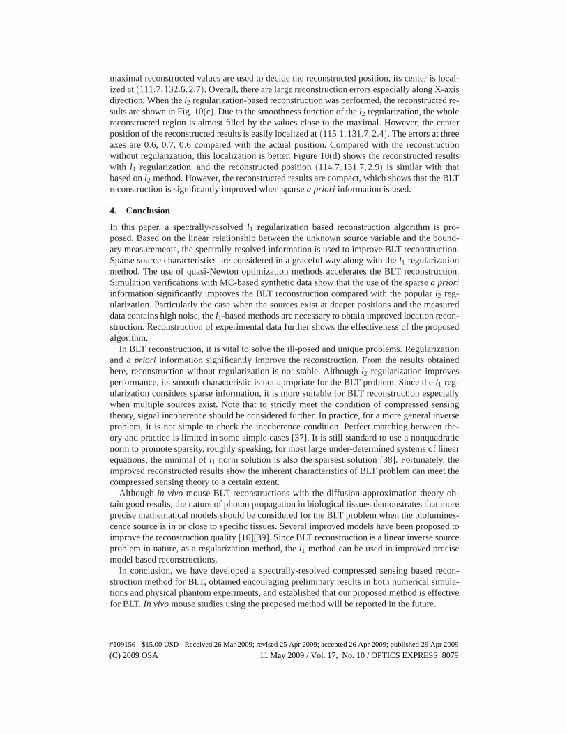
maximal reconstructed values are used to decide the reconstructed position, its center is local-ized at (111.7,132.6,2.7). Overall, there are large reconstruction errors especially along X-axisdirection. When the l2 regularization-based reconstruction was performed, the reconstructed re-sults are shown in Fig. 10(c). Due to the smoothness function of the l2 regularization, the wholereconstructed region is almost filled by the values close to the maximal. However, the centerposition of the reconstructed results is easily localized at (115.1,131.7,2.4). The errors at threeaxes are 0.6, 0.7, 0.6 compared with the actual position. Compared with the reconstructionwithout regularization, this localization is better. Figure 10(d) shows the reconstructed resultswith l1 regularization, and the reconstructed position (114.7,131.7,2.9) is similar with thatbased on l2 method. However, the reconstructed results are compact, which shows that the BLTreconstruction is significantly improved when sparse a priori information is used.

4. Conclusion

In this paper, a spectrally-resolved l1 regularization based reconstruction algorithm is pro-posed. Based on the linear relationship between the unknown source variable and the bound-ary measurements, the spectrally-resolved information is used to improve BLT reconstruction.Sparse source characteristics are considered in a graceful way along with the l1 regularizationmethod. The use of quasi-Newton optimization methods accelerates the BLT reconstruction.Simulation verifications with MC-based synthetic data show that the use of the sparse a prioriinformation significantly improves the BLT reconstruction compared with the popular l2 reg-ularization. Particularly the case when the sources exist at deeper positions and the measureddata contains high noise, the l1-based methods are necessary to obtain improved location recon-struction. Reconstruction of experimental data further shows the effectiveness of the proposedalgorithm.

In BLT reconstruction, it is vital to solve the ill-posed and unique problems. Regularizationand a priori information significantly improve the reconstruction. From the results obtainedhere, reconstruction without regularization is not stable. Although l2 regularization improvesperformance, its smooth characteristic is not apropriate for the BLT problem. Since the l1 reg-ularization considers sparse information, it is more suitable for BLT reconstruction especiallywhen multiple sources exist. Note that to strictly meet the condition of compressed sensingtheory, signal incoherence should be considered further. In practice, for a more general inverseproblem, it is not simple to check the incoherence condition. Perfect matching between the-ory and practice is limited in some simple cases [37]. It is still standard to use a nonquadraticnorm to promote sparsity, roughly speaking, for most large under-determined systems of linearequations, the minimal of l1 norm solution is also the sparsest solution [38]. Fortunately, theimproved reconstructed results show the inherent characteristics of BLT problem can meet thecompressed sensing theory to a certain extent.

Although in vivo mouse BLT reconstructions with the diffusion approximation theory ob-tain good results, the nature of photon propagation in biological tissues demonstrates that moreprecise mathematical models should be considered for the BLT problem when the biolumines-cence source is in or close to specific tissues. Several improved models have been proposed toimprove the reconstruction quality [16][39]. Since BLT reconstruction is a linear inverse sourceproblem in nature, as a regularization method, the l1 method can be used in improved precisemodel based reconstructions.

In conclusion, we have developed a spectrally-resolved compressed sensing based recon-struction method for BLT, obtained encouraging preliminary results in both numerical simula-tions and physical phantom experiments, and established that our proposed method is effectivefor BLT. In vivo mouse studies using the proposed method will be reported in the future.


Acknowledgments

We gratefully thank Dr. Richard Taschereau for his useful discussion about parallel Monte Carlomethod. This work is supported by the NIBIB R01-EB001458, NIH/NCI 2U24 CA092865cooperative agreement, DE-FC02-02ER63520 grants, NSF DMS 0312222, ONR N00014-06-1-0345, NSF CCF-0528583 and the Project for the National Basic Research Program of China(973) under Grant No. 2006CB705700.


source reconstruction for spectrally-resolved bioluminescence ... · source reconstruction for...

Documents