Some New Experiments on the Colorimetric Evaluation of Whiteness

S.V. VAECK

Laboratoire central Ministere des Affaires economiques Rue de la Senne, 17A B 1000 Brussels Belgium

In order to confirm and extend earlier work on the colori- metric evaluation of whiteness, different series of white textiles, each of constant reflectance, varying from Y = 96 to Y = 70, are studied. A study of the Ciba-Geigy white scale is also included.

Earlier predictions about the shape of the equi-whiteness surfaces in the x, y, Y colour space are confirmed and refined. As a result it is established that our original method used as such (using a diagram in the x, y chromaticity chart) or as adapted jbr numerical computation by Ganz, is applicable to nearly all white textiles, with or without FWAs. Only if shading dyes are used can the colour point trnnsgress the optimum whiteness point corresponding to the reflectance of the material. In such cases it is necessary to use equi-whiteness ellipses around the optimum point, whose position in the chromaticity diagram varies nearly linearly with reflectance.

it is also found that catastrophe theory applies to whiteness perception in the vicinity of the optimum whiteness axis in colour space. This means that the whiteness of a given colour in this domain can have a high and a low value, according to circumstances.

Introduction Although the distinction between white and black is the first and most fundamental colour perception [ 11 , until about 1964 surprisingly little was known about the perception of whiteness, and much of what was assumed to be evident was in fact wrong. A complete review of the literature up to 1965 has been published [2-41.

At that time, our experiments with fluorescent and non-fluorescent white textiles [2-41 first corrected this situation; they enabled us to propose the following laws, which since then have gradually been accepted by subsequent investigators. 1 . At any given level of luminance and for all normal

observers, the chromaticity corresponding to the highest whiteness perception is never identical with thc achromatic colour. It is always to the blue or purple side of the achromatic point (achromatic being taken here in the colorimetric sense).

2. As the level of luminance increases, the optimum whiteness chromaticity moves away from the vicinity of the achromatic point and towards the spectrum colour of wavelength about 470 nm. The set of these optimum whiteness points at different luminances defines an opti- mum whiteness curve in colour space.

3 . Distinct differences in whiteness perception exist between

normal observers. However, it is possible to agree on a standard observer for whiteness perception, who is defined by a standard optimum whiteness curve. Among actual observers, the optimum whiteness curve can be slightly displaced in the red direction, relative to the standard curve, (red-preferent observers) or in the green direction (green-preferent observers).

4. For object (fluorescent) colours under normal daylight illumination (D 65), the orthogonal projection of the standard optimum whiteness curve on the CIE chro- maticity diagram is, for all practical purposes, a straight line between a point near the achromatic point and the spectrum colour point of wavelength about 470 nm. This line can be called the optimum (or preferred) whiteness axis in the chromaticity diagram.

5. At high luminance factor (or diffuse reflectance)* values (y>90), the highest whiteness of fluorescent object colours realizable in practice, viewed under normal day- light illumination, is still below that of the (virtual) optimum whiteness point corresponding to the luminance factor, which means that this optimum whiteness point must be a more saturated blue than the whitest fluorescent object colours which can be realized in practice (excitation purity about 14%), when observed under normal daylight illumination.

For lower luminance factor values, it is possible to reach and bypass the optimum whiteness point, which means that in those cases the perception of blueness prevails over the perception of whiteness. The transition from whiteness perception to colour perception is often a catastrophic event. In other words, the limit is not strictly defined: it oscillates according to the direction from which it is approached as well as depending on the surrounding field.

6. For all observers a small departure of the chromaticity from their optimum whiteness axis, either in the green or in the red direction, luminance remaining constant, pro- duces a sharp decrease in the perceived whiteness. This means that in the chromaticity diagram the equi-whiteness curves at constant luminance must be elongated (irregular) ellipses.

From all this it can be seen that, in its most general form, the relation between whiteness and colour specification is very complex indeed. However, for practical purposes, limitation to the evaluation of the whiteness of textiles, plastics and papers dyed with commercial fluorescent whitening agents (FWA), having a high luminance factor, shows that the calculation of a whiteness value is relatively simple. It is sufficient to add the lightness contribution, measured as Y (%), to the chromaticity contribution, read from a chromaticity diagram ad hoc, in which the equi-whiteness lines are degenerate hyperbolae * The photometric equivalent of the visual perception o f lightness is,

strictly speaking, the luminance factor. However, many instruments use an integrating sphere and they measure diffuse reflectance, or something near to it.

262 JSDC July 1979

(representing the intersection of the hyperboloid whiteness surfaces in colour space and a plane of constant luminance factor).

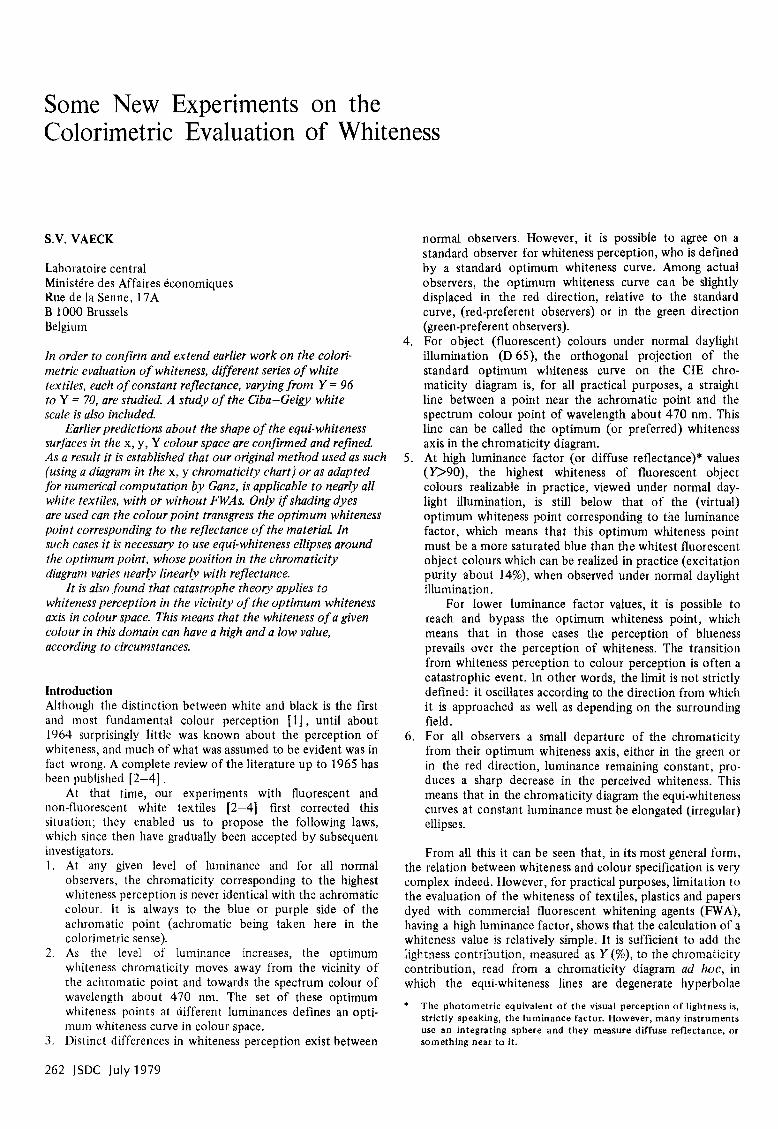
Figure 1 shows these equi-whiteness lines, based on our earlier results, recalculated for D 65 as achromatic point in the 1964 CIE (xl o, y1 o ) - chromaticity diagram.

0.3 1

0.3:

A 0.32

0.3

0.30

4-12:

u : T : 0 :

0 :

0.29 0.30 0.31 0.32 X

chromaticity points of steps 4 to 12 of the Ciba-Geigy plastic white scale dyeing of 0.5% Uvitex C F conc. new on bleached cotton dyeing of 2% Tinopal WHN on white Perlon as measured with the Zeiss D F C 5 as measured with the Zeiss RFC 3

Figure 1 - Equi-whiteness lines in the 1964 CIE ( x l o , y o)-chromaticity diagram for Source D 65 and measurement with the Zeiss DFC 5, based on our 1964 experiments.

It should be pointed out that the shape of this diagram differs significantly from the one csnstructed in the 1931 CIE (x, y ) diagram. I t also depends on the instrument used for the measurements. In the case of Figure 1 this is the Zeiss DFC 5.

If another instrument is used, the diagram should be adapted accordingly, because no two different types of instrument have the same u.v.-content in the light falling on the specimen. For non-fluorescent samples this is without importance, but for fluorescent samples the chromaticities may be quite different. To illustrate this the chromaticity point of the Ciba-Geigy scale, as measured with the Zeiss RFC 3 spectrophotometer, have been plotted. It is at once apparent

that the illuminant in this instrument emits much less in the u.v.-range so that the chromaticity points of the fluorescent samples are nearer the achromatic point. F x non-fluorescent samples (no. 1-5) on the other hand, the chromaticity points as measured by both instruments are very nearly identical. These results are similar to those obtained by Ganz [51.

The preferred whiteness axis has been drawn through the achromatic point (x = 0.31375, y = 0.33086), although it is known that it passes slightly to the red side of this point (for the standard whiteness observer). However, for the evaluation of FWA-whitened textiles the distinction is immaterial. T h e other point defining the axis is the colour point of step 12 of the Ciba-Geigy plastic white scale (in this case it has the values x = 0.2919, y = 0.3034). The equivalent luminance (%) is 80, which means that step 12, which has a reflectance (%) of about 89, measured with the Zeiss DFC 5, has a whiteness equivalent to that of the perfect diffuser, when the latter is illuminated with an illuminance having the relative value 80 t 89 = 169 when the illuminance on step 12 has the value 100.

Alternatively, the preferred axis can also be defined by the colour point of a dyeing of 0.5 % Uvitex CF conc. new (CGY) on bleached cotton, which has an equivalent luminance of 74, or by that of a dyeing of 2% Tinopal WHN (CCY) on white Perlon, with an equivalent luminance of 92.5, which is the highest value encountered by us to-date.

In an earlier diagram, the straight eyui-whiteness lines met at the preferred whiteness axis, which implied a discontinuity in aV/aH(V = whiteness, H = hue). To avoid this the tips have been rounded, as shown in Figure 1. The preferred whiteness axis intersects the spectrum locus at wavelength 467.5 nm.

This method has been adapted for numerical computation by Ganz [5j with the possibility of shifting the preferred whiteness axis according to the preference of the observer, although in practise hd = 470 nm is nearly always chosen.

The main drawback of the method is that the conceptual transparency of the diagram is lost.

Mechanical use of Canz’s mathematical fxmulae may lead to a loss of insight into the colorimetric relations.

Unsolved Problems Although the practical problem of evaluating the whiteness of textiles, papers and plastics dyed exclusively with FWAs has been solved by this method and its development by Ganz, the general problem of defining the equi-whiteness surfaces in colour space (at least in that part of it where the concept of whiteness can have a meaning) remains largely unsolved.

In particular, the exact shape of the optimum whiteness curve in colour space, i.e. the location 3f the optimum whiteness point at each luminance factor level, is still a subject of dispute, At very high luminance factor levels ( 0 9 0 ) the optimum whiteness point has a blue satxration which is without doubt higher than 14%. For very low levels (D80) our results have shown that it must lie near the achromatic point. Thielert and Schliemann 161 have published results which seem to confirm that for intermediate luminance factor levels it occupies an intermediate position. As a result, it has been suggested [7] that the optimum whiteness curve is a parabolic curve in the x , y , Y colour space.

In order to clarify this problem further, the relation between the visual evaluation of whiteness and the color- imetric specifications of a number of white textiles of

JSDC July1979 263

different chromaticities at different reflectance levels have been studied, and the Ciba-Geigy white scale has been investigated.

Experimental

APPARATUS

Zeiss DFC 5 Automatic Colorimeter All measurements were made on this instrument, which is a three-filter tristimulus colorimeter with xenon arc illumination and d/8" geometry.

The filters were placed in the light beam reflected from the specimen, an arrangement which made the instrument suitable for the measurement of fluorescent materiJs (but only for Source D 65). An on-line HF' 9815 computer was used to calculate the CIE 1964 tristimulus values XI o,.Y1 o,Z1 0 for Source D 65.

All measurements were made with a gloss trap, so that diffuse reflectance was measured.

Zeiss RFC 3 Spectrophotorneter This instrument was used when a recording of the spectral reflectance curves was required. It is an abridged spectrophoto- meter with 24 interference filters; the illumination and geometry are similar to that of the DFC 5, but the U.V. content of the light is less, as pointed out earlier. An on-line PDP 8/E computer was used to calcllate the tristimulus values, colour differences, etc., for any chosen illuminant or observer. Here also a gloss trap was used.

SPECIMENS

Ciba-Geig-y Plastic White Scale This comprises 12 steps rated from -20 to 210 on a scale which is claimed to be visually uniform [ 5 ] . Our scale was a recent one (1977) which was found to differ significantly from older issues [8].

FWA-treated Textiles ofMaximum Reflectance ( Y = 94 +I) B1 : 2% Tinopal WHN (CCY) on white nylon 6 B2 : 1.5% Blankophor CL (BAY) on bleached cotton B3 : 1.5% Tiponal RP (CCY) on white nylon 6 B4 : 0.5% Blankophor CL (BAY) on bleached cotton B5 : 0.5% Uvitex CF conc. new (CCY) on bleached cotton.

TABLE 1

Colorimetric Specifications and Visual Evaluation of Samples of Series B ( Y = 94.2 k0.7)

Sample Colorimetric specifications (D 65", 10" observer,

Zeiss DFC 5) Y X Y

B1 94.9 0.2888 0.2988 B2 94.9 0.2920 0.3003 B3 94.8 0.2923 0.3026 B4 95.9 0.2938 0.3061 B5 93.5 0.2938 0.3051

Eleven FWA-treated Cotton Fabrics (Cl to C11) Of these, six dyed red, blue or green, all specimens having a medium reflectance ( Y = 87.5 +2).

Ten Non-fluorescent Cotton Fabrics (Dl to DIO) These were dyed with small quantities of different dyes, all specimens showing a low reflectance (Y = 69 + 2 ) .

All the fabric specimens measured 6 x 10 cm, 8 layers being superimposed.

VISUAL ASSESSMENT The visual assessment of whiteness was made by three observers R, B, G, with normal colour vision, showing a slight but distinct red-, blue- and green-preference, respectively, in 3 viewing booth equipped with an Osram XBO 162 xenon arc lamp in a Siemens CL 10 G housing.

The background was a light grey ( Y = 50), except when series D was assessed. In that case it was necessary to use a black background (Y * 4) in order to enable the observers tcr make whiteness judgments.

All the samples of a given series were compared with one another (pair comparison method), the judgment being forced (no equality admitted).

The two samples of each pair were presented side by side. their relative positions being changed frequently (this is an import ant precaution).

Results and Discussion

FABRICS OF MAXIMUM REFLECTANCE The colorimetric specifications (for D 65 and the 10" observer, as measured with the DFC 5) of the samples of series B and their visual rank order under xenon lamp illumination are given in Table 1.

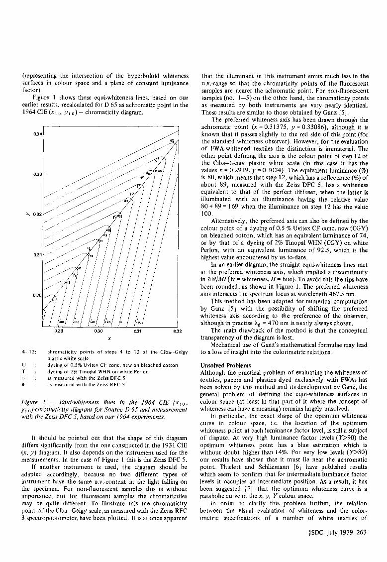
Figure 2 shows the chromaticity points of these samples. I t can be seen that, for these samples, the three observers agree in their ranking.

They equate whiteness with blue saturation, up to the limit of the whitest sample, although this has a saturation of about 14%. As a result, formulae such as the one of Berger, which equate whiteness with blue saturation, are applicable. Our method, based on the diagram of Figure 1, also gives valid results, but the preferred whiteness axis should be moved a little to the red side, in order to obtain the best correlation

Visual rank order Whiteness Value: from our from Berger

1964 diagram formula [9] Observer R B G Average 1 1 1 1 187.5 188.4 2 2 2 2 175 178.7 3 3 3 3 175 174.8 5 5 5 5 166.5 165.2 4 4 4 4 167.5 167.5

264 JSDC July 1979

0.31

A

a3c

Figure 2 - Chromaticity points o f the samples o f series B in the 1964 CIE chromaticity diagram. Source D 65 and measurement with Zeiss DFC 5. Equi-whiteness lines from Fipure 1

with visual assessment. Besides, this experiment shows that the optimum whiteness point, at the 94% reflectance level, corresponds to a blue saturation higher than 14%.

However, there are reasons to believe that it cannot be much higher, under daylight illumination, as the blue tint of the whitest sample tends to become apparent to our observers under certain daylight viewing conditions.

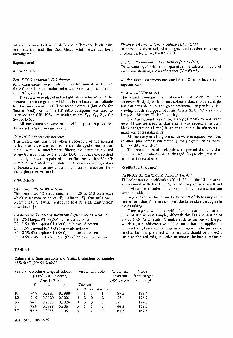
The present results confirm our earlier ones. They are also in agreement with the latest experiments of Berglund and Stenius [lo], if their experiment I is considered, in which 30 paper samples were evaluated by 30 observers, an undyed sample serving as reference standard. Figure 3 is a plot of the equi-whiteness lines corresponding to the average judgment of these observers for the 10 samples of highest blue saturation. It can be seen that they confirm the conclusions stated above, although it is apparent that the shape of the equi-whiteness lines in the chromaticity diagram is elliptical rather than hyperbolical. Minor deviations occur because the reflectance of the samples is not constant, but varies from 90.5 to 97.6, according to measurements made by Berger on an Elrepho colorimeter [ 111 . The preferred whlteness axis derived from these data lies to the red side of that shown in Figures 1 and 2.

a32

A

0.31

/

0.30 0.31

X

Figure 3 - Chromaticity points of the 19 samples (ojhighest blue saturation) studied by Berglund and Stenius [ l o / and average equi-whiteness lines for their 30 observers (experiment Ij; 1964 CIE chromaticity diagram, Source D 65, measure- ments ivith Zeiss Elrepho b y Berger [ 1 11.

If Figure 1 is superimposed on Figure 3 in such a way that the preferred whiteness axis coincides with the one derived from the visual evaluation, the whiteness values calculated according to our method show a correlation r = 0.9 16 with the average judgment of 30 observers, whereas, for example, for the Berger formula, r = 0.785.

Unfortunately, the samples of Berglund and Stenius do not attain the high saturation values of series B.

FABRICS OF MEDIUM REFLECTANCE (SERIES C) The colorimetric specifications and the visual rank order of the samples of series C are given in Table 2 .

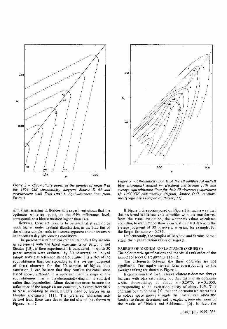
The differences between the three observers are not significant. The equi-whiteness lines corresponding to the average ranking are shown in Figure 4.

It can be seen that for this series whiteness does not always increase with blue saturation, but that there is an optimum white chromaticity, at about x = 0.2975, y = 0.3050, corresponding to an excitation purity of about 10%. This confirms our hypothesis [7] that the optimum whiteness axis in colour space moves towards the neutral axis when the luminance factor decreases, and it explains, inter alia, some of the results of Thielert and Schliemann [6]. In fact, the

JSDC July1979 265

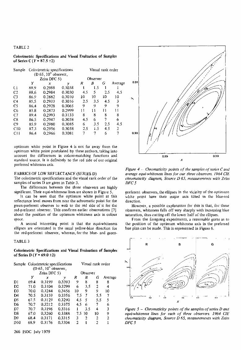
TABLE 2

Colorimetric Specifications and Visual Evaluation of Samples of Series C (Y = 87.5 +2)

Sample Colorimetric specifications Visual rank order (D 65, 10" observer,

Zeiss DFC 5) Observer Y X Y R B G Average 03'

c1 88.9 0.2988 0.3038 1 1.5 1 1 c2 88.6 0.2984 0.3030 4.5 5 2.5 4.5 c 3 86.9 0.2882 0.3010 10 10 10 10 c4 85.5 0.2933 0.3016 2.5 3.5 4.5 3 c5 86.4 0.2928 0.3065 9 9 9 9 C6 85.8 0.2873 0.2999 11 11 11 11 c7 89.4 0.2993 0.3133 8 8 8 8 C8 86.5 0.2947 0.3058 4.5 6 7 6 c9 85.9 0.2980 0.3085 6 3.5 2.5 4.5 C10 87.3 0.2956 0.3058 2.5 1.5 4.5 2

A

030

C11 86.4 0.2966 0.3081 7 7 6 7 0.30

optimum white point in Figure 4 is not far away from the optimum white point postulated by these authors, taking into account the differences in colour-matching functions and 0 29 standard source. It is definitely to the led side of our original X

preferred whiteness axis.

FABRICS OF LOW REFLECTANCE (SERIES D) The colorimetric specifications and the visual rank order of the samples of series D are given in Table 3.

The differences between the three observers are highly significant. Their equi-whiteness lines are shown in Figure 5.

It can be seen that the optimum white point at this reflectance level moves from near the achromatic point for the green-preferent observer to well to the red side of it for the red-preferent observer. This confirms earlier observations [7] about the position of the optimum whiteness axis in colour space.

ellipses are orientated in the usual yellow-blue direction for the red-preferent observer, whereas, for the blue- and green-

Figure 4 - Chromaticity points of the samples of series Cutid average equi-whiteness lines for our three observers. 1964 CIE chromaticity diagram, Source D 65, measurements with Zeiss DFC 5

preferent observers, the ellipses in the vicinity of the optimum white point have their major axis tilted in the blue-red direction.

However, a possible explanation for this is that, for these observers, whiteness falls off very sharply with increasing blue saturation, thus cutting off the lower half of the ellipses.

From the foregoing experiments, a reasonable guess as to A second interesting point is that the eyui-whiteness the position of the optimum whiteness axis in the preferred

hue plan can be made. This is represented in Figure 6.

TABLE 3

Colorimetric Specifications and Visual Evaluation of Samples of Series D (Y = 69.0 k2)

Sample Colorimetric specifications Visual rank order (D 65, 10" observer,

Zeiss DFC 5) Observer Y X y R B G Average

D1 69.4 0.3199 0.3393 9 8 8 8 D2 71.0 0.3104 0.3299 6 3.5 2 4 D3 70.G 0.3244 0.3456 10 9 9 10 D4 70.5 0.3159 0.3356 7.5 7 5.5 7 D5 67.5 0.3129 0.3290 4.5 5 5.5 5 D6 70.7 0.3212 0.3375 4.5 6 7 6 D7 70.7 0.3196 0.3316 1 3.5 4 3 D8 67.0 0.3260 0.3388 7.5 10 10 9 D9 68.4 0.3171 0.3315 3 2 2 2 D10 68.9 0.3176 0.3304 2 1 2 1

t . . i--_

111 0 3 1 0 11 011 011 01)

X

Figure 5 - Chromaticity points of the samples of series D and equi-whiteness lines for each o f three observers. 1964 ClE chromaticity diagram, Source D 65, measurements with Zeiss DFC 5

266 JSDC July 1979

461 nm c,

15 10 5

Excitation purity, %

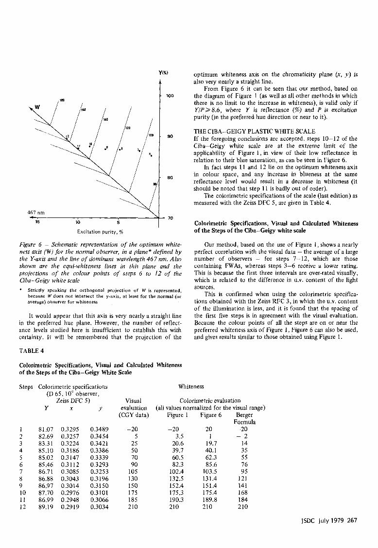
Figure 6 - Schematic representation of the optimum white- ness axis (W) for the normal observer, in a plane* defined by the Y-axis and the line of dominant wavelength 467 nm. Also shown are the equi-whiteness lines in this plane and the projections of the colour points of steps 6 to 12 of the Ciba-Geigy white scale * Strictly speaking the orthogonal projection of W is represented,

because W does not intersect the y-axis, at least for the normal (or average) observer for whiteness

It would appear that this axis is very nearly a straight line in the preferred hue plane. However, the number of reflect- ance levels studied here is insufficient to establish this with certainty. I t will be remembered that the projection of the

optimum whiteness axis on the chromaticity plane (x, y ) is also very nearly a straight line.

From Figure 6 it can be seen that our method, based on the diagram of Figure 1 (as well as all other methods in which there is no limit to the increase in whiteness), is valid only if YIP28.6, where Y is reflectance (%) and P is excitation purity (in the preferred hue direction or near to it).

THE CIBA-GEIGY PLASTIC WHITE SCALE If the foregoing conclusions are accepted, steps 10-12 of the Ciba-Geigy white scale are at the extreme limit of the applicability of Figure 1, in view of their low reflectance in relation to their blue saturation, as can be seen in Figure 6.

In fact steps 11 and 12 lie on the optimum whiteness axis in colour space, and any increase in blueness at the same reflectance level would result in a decrease in whiteness (it should be noted that step 11 is badly out of order).

The colorimetric specifications of the scale (last edition) as measured with the Zeiss DFC 5, are given in Table 4.

Colorimetric Specifications, Visual and Calculated Whiteness of the Steps of the Ciba-Geigy white scale

Our method, based on the use of Figure 1, shows a nearly perfect correlation with the visual data - the average of a large number of observers - for steps 7-12, which are those containing FWAs, whereas steps 3-6 receive a lower rating. This is because the first three intervals are over-rated visually, which is related to the difference in U.V. content of the light sources.

This is confirmed when using the colorimetric specifica- tions obtained with the Zeiss RFC 3, in which the U.V. content of the illumination is less, and it is found that the spacing of the first five steps is in agreement with the visual evaluation. Because the colour points of all the steps are on or near the preferred whiteness axis of Figure 1, Figure 6 can also be used, and gives results similar to those obtained using Figure 1.

TABLE 4

Colorimetric Specifications, Visual and Calculated Whiteness of the Steps of the Ciba-Geigy White Scale

Steps

1 2 3 4 5 6 7 8 9 10 11 12

Colorimetric specifications Whiteness (D 65, 10" observer,

Zeiss DFC 5 ) Visual Colorimetric evaluation Y X

81.07 0.3295 82.69 0.3257 83.31 0.3224 85.10 0.3186 85.02 0.3147 85.46 0.3112 86.71 0.3085 86.88 0.3043 86.97 0.3014 87.70 0.2976 86.99 0.2948 89.19 0.2919

Y

0.3489 0.3454 0.3421 0.3386 0.3339 0.3293 0.3253 0.3196 0.31 50 0.3101 0.3066 0.3034

evaluation (CGY data)

-20 5

25 50 70 90

105 130 150 175 185 210

(all values normalized for the visual range) Figure 1 Figure 6 Berger

-20 -20 -20 3.5 1 - 2

20.6 19.7 14 39.7 40.1 35 60.5 62.3 55 82.3 85.6 76

102.4 103.5 95 132.5 131.4 121 152.4 151.4 141 175.3 175.4 168 190.3 189.8 184 210 210 2 10

Formula

JSDC July1979 267

The Berger formula is less satisfactory. The overall correlation coefficients of the visual and colorimetric ratings are 0.998 or higher, but this is misleading. A better measure of the goodness of fit is obtained when the correlation coeffi- cients of the successive spacings of the different steps are calculated. These are 0.64 resp. 0.72 for our method described here, and 0.49 for the Berger method. If considering only steps 5-12, excluding the samples containing a yellow dye, the correlation Coefficients of the intervals are improved -0.74, resp. 0.82 for our method, and 0.86 for the Berger method. These differences illustrate the problems posed by a scale comprising both fluorescent and non-fluorescent samples.

In conclusion, taking into account the large uncertainties inherent in all visual ratings, and the supplementary problems encountered when colour differences between both fluores- cent and non-fluorescent samples must be evaluated, the method described in this paper agrees well with the visual assessment of the Ciba-Geigy white scale. However, it must be remembered that the samples of this scale have a rather low reflectance, near to the limit of validity of our method established for textile materials of high reflectance.

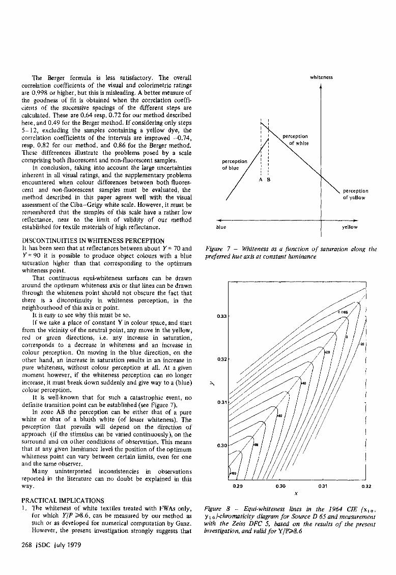
DISCONTINUITIES IN WHITENESS PERCEPTION It has been seen that at reflectances between about Y = 70 and Y = 90 it is possible to produce object colours with a blue saturation higher than that corresponding to the optimum whiteness point.

That continuous equi-whiteness surfaces can be drawn around the optimum whiteness axis or that lines can be drawn through the whiteness point should not obscure the fact that there is a discontinuity in whiteness perception, in the neighbourhood of this axis or point.

It is easy to see why this must be so. If we take a place of constant Y in colour space, and start

from the vicinity of the neutral point, any move in the yellow, red or green directions, i.e. any increase in saturation, corresponds to a decrease in whiteness and an increase in colour perception. On moving in the blue direction, on the other hand, an increase in saturation results in an increase in pure whiteness, without colour perception at all. At a given moment however, if the whiteness perception can no longer increase, it must break down suddenly and give way to a (blue) colour perception.

It is well-known that for such a catastrophic event, no def i i te transition point can be established (see Figure 7).

In zone AB the perception can be either that of a pure white or that of a bluish white (of lesser whiteness). The perception that prevails will depend on the direction of approach (if the stimulus can be varied continuously), on the surround and on other conditions of observation. This means that at any given luminance level the position of the optimum whiteness point can vary between certain limits, even for one and the same observer.

Many uninterpreted inconsistencies in observations reported in the literature can no doubt be explained in this way.

blue

PRACTICAL IMPLICATIONS 1. The whiteness of white textiles treated with FWAs only,

for which YIP 28.6, can be measured by our method as such or as developed for numerical computation by Ganz. However, the present investigation strongly suggests that

f

yellow

whiteness

perception of yellow

\

Figure 7 - Whiteness as a function of saturation along the preferred hue axis at constant luminance

I '

0.29 0.30 0.31 0.32 X

Figure 8 - Equi-whiteness lines in the 1964 ClE ( x l o , y1 o)-chromaticity diagram for Source D 65 and measurement with the Zeiss DFC 5, based on the results of the present investigation, and valid for YjP28.6

268 JSDC July 1979

the preferred whiteness axis shown in Figure 1 should be displaced to the right (in the red direction) by a distance corresponding to about 0.003 in x , for measurements with the Zeiss DFC 5 or RFC 3. The angle between this axis and the equi-whiteness lines appears about right in the vicinity of the preferred axis; at distances larger than about 0.005 in x, they tend to run more in parallel with the axis, but such colours are rarely, if ever, found in practice. The spacings of the equi-whiteness lines (and the parameters in the equations of Ganz) should be adapted to the measuring instrument being used, those given in Figure 1 being valid for the DFC 5. Taking all this into account, an improved diagram (Figure 8) to that of Figure 1 has been con- structed. For white textiles containing shading dyes, the position of the colour point with respect to the optimum whiteness axis in the x,y,Y colour space should be ascertained first. If the colour point lies above or on this axis (Y/P 238.6) our method and that of Ganz can be used. If not (Y/P<8.6) equi-whiteness ellipses such as those shown in Figure 4 must be used, the position of the centre of the ellipses being defmed by the reflectance of the sample, in such a way that it coincides with the intersection of the optimum whiteness axis in colour space and the plane Y = constant. For colour points in the immediate vicinity of the optimum whteness axis in colour space, the whiteness value cannot be assessed unambiguously: it can oscillate between a high value (pure white perception) and a low value (bluish-white perception).

Note An optimum whiteness axis similar to the one shown in Figure 6 was proposed by McConnell [121, based on work with tinted papers. However, its position is shifted to the right, possibly because of the unusual lighting conditions used by the author.

References

1. Berlin and Kay, ‘Basic color terms. Their universality and evolution’. (Berkeley: University of California Press, 1969).

2. Vaeck and Van Lierde, Ann. Sci. Textiles Belges, No. 1 (1964) 7.

3. Idem, ibid., No. 3 (1964) 7. 4. Vaeck, ibid., No. 1 (1966) 95. 5. Ganz, Appl. Optics, 15 (1976) 2039. 6. Thielert and Schliemann, J. Opt. SOC. h e r . , 63 (1973)

7. Vaeck, Ann. Sci. Textiles Belges, No. 2 (1975) 184. 8. Anders, J.S.D.C., 84 (1968) 125. 9. Berger, Farbe, 8 (1959) 187.

1607.

10. Berglund and Stenius, Report No. 5 of the CIE TC-1.3

11. Berger, Report No. 2 of the CIE TC-1.3 (Colorimetry)

12. McConnell, Roc . of the First International Colour Meet-

(Colorimetry) subcommittee on whiteness (1975).

subcommittee on whiteness (1975).

ing, Stockholm, 1969 (Musterschmidt, Gottingen).

(MS received 1 7 October I 9 78)

JSOC July1979 269