Solving Differential Equations on 2-D Geometries with Matlab

Joshua Wall∗

Drexel UniversityPhiladelphia, PA 19104

(Dated: April 28, 2014)

I. INTRODUCTION

Here we introduce the reader to solving partial differ-ential equations (PDEs) on 2 dimensional geometries us-ing the Matlab package PDE Tool. This robust packagesolves PDE’s using a finite element method. For moreinformation on the finite element method, I refer you toAllyson or Dr. Gilmore 1. If you want a cock-a-maymieexplanation, you’re welcome to come find me 2.

II. SOLVING THE EIGENVALUES AND EIGENVECTORSON A WASHER

A. Getting PDE Tool Ready to Go

Okay, so lets look at solving the actual problem given,which is solving the diffusion equation on a circularwasher:

−∇ · (c ∗ ∇u) + a ∗ u = λ ∗ d ∗ u

where c, a and d are constants and u is the solution. ais generally called k2 and d is often called ρ, the weight-ing function. We wish to solve the Schrodinger equationspecifically on the washer, so we have:

h2

2m∇2ψ(r, θ) = Eψ(r, θ)

with the boundary conditions that ψ = 0 at the radialedges of the washer.

We will let our problem have ”natural units,” so h =m = 1. So for us c = 0.5, a = d = 1.0. We’ll need thislater.

Start Matlab, then start the PDE tool by either find-ing in under the Apps tab or typing pdetool into the com-mand window. You will be greeted with a blank screenunder a row of buttons.

The screen is where we will draw our geometry, butfirst lets make it easier with a few settings. Click on Op-tions, and turn on the Grid and Snap. Snap makes our

∗ joshua.e.wall@gmail.com1 Added to the list of people that know more than I do.2 Bring alcohol.

drawings pop onto the grid lines you now see. Next selectgrid spacing and set it to draw grid lines at every integerin x and y. Also define the grid to go from [−12 12] forboth axes. Then click on Axes Equal to get the propershape of the grid. Finally, click on Solve, then Parame-ters and set the Eigenvalue range to go from [0 1]. Ifthis range is too large it will time out while trying tosolve for the eigenvalues.

B. Drawing the Geometry

Now that we have set the proper parameters, we candraw our geometry. Matlab uses a union/subtractionmethod to make complex geometries on the space. Forinstance, you can draw a disk, then draw a rectanglethrough it.

To draw a circle/ellipse, you pick either button that hasan ellipse on it. The button with the ’+’ in the centermeans it draws starting the center at the point you click,while the other starts an edge of the shape where youclick. The same goes for the rectangles.

You will see in the Set formula box that a combinationof letters and numbers appears for each shape as youdraw them, like for an ellipse E1 or for a rectangle R2.If these label your disk and rectangle, you can define yourproblem on both surfaces with E1+R2 or just in the areaof the disk outside of the rectangle with E1−R2.

Here we want a washer. So first draw a circle withradius 12 by clicking on the button of an ellipse with the’+’ in it, then clicking at the origin and dragging thecircle out to a radius of 12. Then do this again for acircle of radius of 5. You should see in the Set formulabox C1 + C2. Change this to C1 − C2, and you havedefined the geometry of a washer.

C. Setting the Boundary Conditions and the Equation

Next we click on the ∂Ω button. This gives the bound-ary conditions, and you now see the washer shape out-lined in red. If you double click any red line, it gives youthe option to select Dirichlet or Neumann boundary con-ditions. The red is Dirichlet, Neumann would be blue.So this is already set to what we want, and no valuesneed to be changed here.

2

FIG. 1 The Matlab PDE Tool

Next click the PDE button, and the choices for thefour different types of PDEs appear. Here Eigenvalue isthe diffusion equation, which is what we want. You willsee settings for the constants we defined before. Simplyset c = 0.5, a = 0.0, and d = 1.0 and your done here.

D. Creating the Mesh and the Solution

Next click on the ∆ button. This makes a mesh on thewasher surface. This mesh is the FEM part of solving theproblem. The initial mesh is fairly coarse, and will resultin a rather coarse solution. Clicking the button withthree ∆s stacked will refine the mesh for a more accuratesolution, but takes longer to calculate. I recommend 3times to make sure you get the proper degeneracy of theeignvalues.

After this, click on the Mesh in the menu bar, followedby Jiggle Mesh. This wiggles the mesh elements to betterfit at the edges and bends in the geometry.

Finally, click the = button to solve the problem.

E. Solutions and Plots

After you click the solve button, Matlab will calcu-late the solution and then the window will change to acolor plot of the first solution. You can then click the

button that looks like a 3-D plot to explore the solu-tions. This will present you with the Plot Selection win-dow. Here you can pick which eigenvector to plot by se-lecting the corresponding eigenvalue from the drop downmenu on the bottom right, then checking which type ofplot you want (color, contour, arrows, deformed mesh,or 3-D height plot). You can pick to plot the solutionu,∇u, |∇u|, or some user defined function of u just asyou would define any Matlab function.

If you simply click the different eigenvalues and thenplot the color plots of u, you will be able to see all of thenormal modes of the problem, including those that havedegenerate eigenvalues.

You can then save the plots or click on Solve in themenu and then Export Solution to export the eigenvaluesand eigenvectors to the main Matlab window for furtherplotting or work. You can also click on File then Save asto save an m-file of the problem and the solutions.

III. MY RESULTS

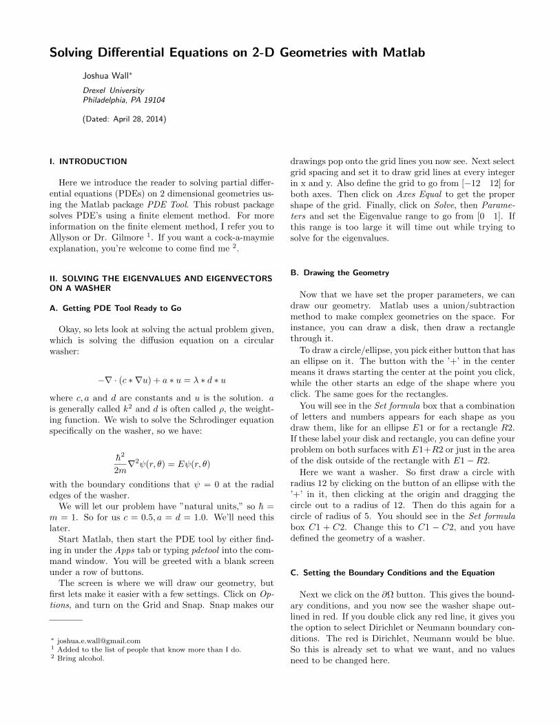
Having explained how to do the calculation, I nowpresent my findings using PDE Tool. Note that I presentthe unitless eigenvalues λ, for the energies multiply theseby h2/m. Here are the first 20 eigenvalues:

3

n λ ∗m/h2

1 0.0989

2 0.1063

3 0.1063

4 0.1283

5 0.1283

6 0.1644

7 0.1644

8 0.2136

9 0.2136

10 0.2748

11 0.2748

12 0.3470

13 0.3470

14 0.4012

15 0.4092

16 0.4092

17 0.4291

18 0.4291

19 0.4334

20 0.4334

The degeneracy in the eigenvalues relates to the ax-ial symmetry of the washer shape. It doesn’t matter if Itravel the washer in the positive or negative θ direction, I

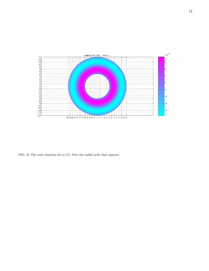
still see the same infinite potentials at the same radii. So Iget an energy for travel clockwise exp(+inθ) and counter-clockwise exp(−inθ). There are two singular eigenvalueshere though, the ground state (n=1) and the fourteenthstate (n=14). These are states that don’t have nodes inthe theta direction, instead they have nodes in the ra-dial r direction. We anticipate these would continue toappear as n gets higher, with each singular eigenvaluecorresponding to an eigenfunction with an additional ra-dial node.

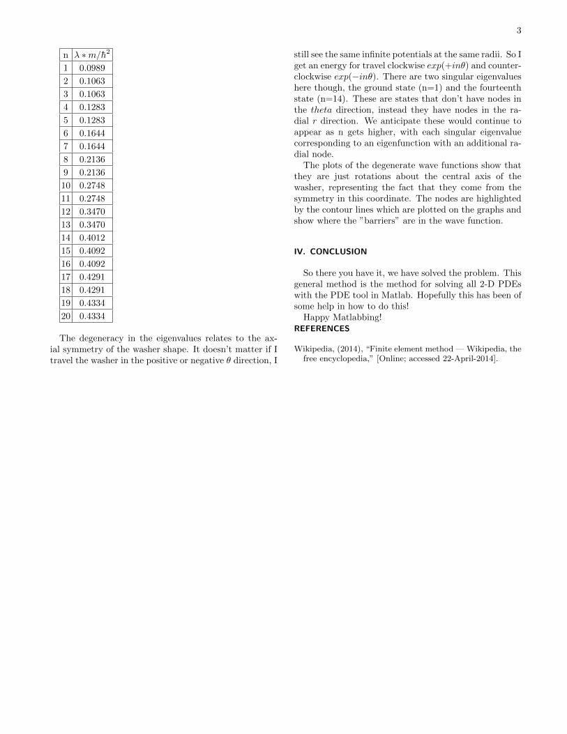
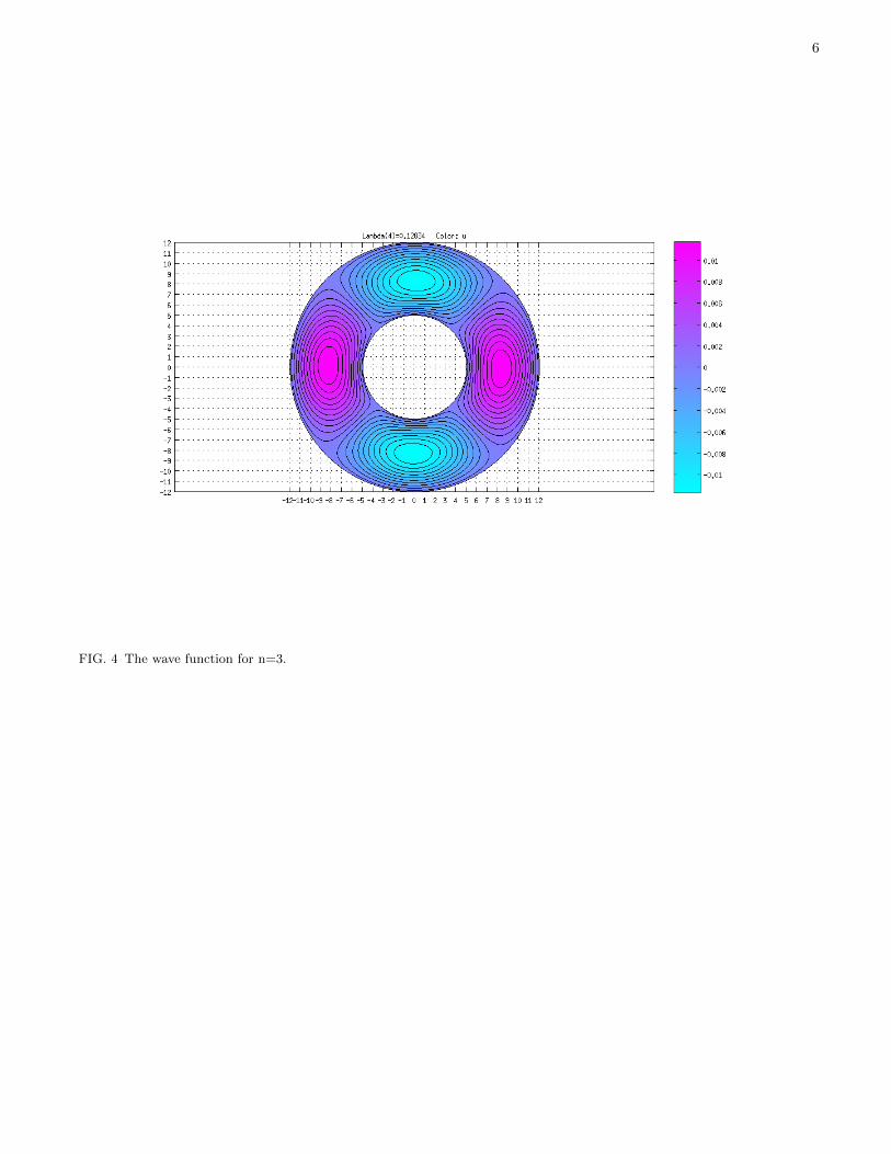
The plots of the degenerate wave functions show thatthey are just rotations about the central axis of thewasher, representing the fact that they come from thesymmetry in this coordinate. The nodes are highlightedby the contour lines which are plotted on the graphs andshow where the ”barriers” are in the wave function.

IV. CONCLUSION

So there you have it, we have solved the problem. Thisgeneral method is the method for solving all 2-D PDEswith the PDE tool in Matlab. Hopefully this has been ofsome help in how to do this!

Happy Matlabbing!REFERENCES

Wikipedia, (2014), “Finite element method — Wikipedia, thefree encyclopedia,” [Online; accessed 22-April-2014].

4

FIG. 2 The wave function for n=1 (ground state).

5

FIG. 3 The wave function for n=2.

6

FIG. 4 The wave function for n=3.

7

FIG. 5 The wave function for n=4.

8

FIG. 6 The wave function for n=5.

9

FIG. 7 The wave function for n=5.

10

FIG. 8 The wave function for n=6.

11

FIG. 9 The wave function for n=7.

12

FIG. 10 The wave function for n=14. Note the radial node that appears.