solidification and compositional convection of a ternary · pdf filesolidification and...
TRANSCRIPT
J. Fluid Mech. (2003), vol. 497, pp. 167–199. c© 2003 Cambridge University Press
DOI: 10.1017/S002211200300661X Printed in the United Kingdom
167
Solidification and compositional convectionof a ternary alloy
By ANDREW F. THOMPSON†, HERBERT E. HUPPERT,M. GRAE WORSTER AND ANNELI AITTA
Institute of Theoretical Geophysics, Department of Applied Mathematics and Theoretical Physics,University of Cambridge, Wilberforce Road, Cambridge CB3 0WA, UK
(Received 14 March 2003 and in revised form 30 June 2003)
We present the results of an experimental study on the solidification of aqueoussolutions of potassium nitrate and sodium nitrate cooled from below. Upon cooling,two distinct mushy layers form, primary and cotectic, separated by an approximatelyplanar horizontal interface. A density reversal between the two mushes causes theresidual liquid in the upper, primary mush to be more buoyant than the melt overlyingit, while the cotectic mush is compositionally stable. The unstable concentrationgradient between the melt and primary mush causes convection that keeps the meltwell-mixed and reduces the concentration gradient to zero after a finite time. Atthis point, the cotectic mush overtakes the primary mush and a transition from aconvective regime to a diffusive regime occurs. Our measurements show that thistransition is rapid and alters the growth rate of the single (cotectic) mush layer thatremains. Concentration measurements taken from within the melt during convectionand from within the mush during the diffusive regime show good agreement with theconcentration evolution predicted by use of the equilibrium ternary phase diagram.We describe a global conservation model for solidification of a ternary alloy in thisregime. Predictions from our model forced with empirical data for the heat andsolute fluxes are in good agreement with the measured data for the interface positionsof the two mushy layers. We also discuss how solid fractions vary with differentmelt concentrations in a non-convecting alloy and examine the influence of verticalsolute transport in the convecting case. The identification of a density reversal in thesolidification of a ternary alloy begins to address the complexities in solidificationprocesses of multi-component alloys.
1. IntroductionThe formation of solids by cooling a liquid melt is an integral part of many natural
and industrial processes. Many of these solidification processes also generate fluidflows that are effective means of heat and mass transport and significantly influencethe structure and growth rate of the solid phase. These fluid motions occur in liquidalloys owing to thermal convection caused by cooling the melt or to compositionalconvection caused by the removal of one or more components from the melt toform the solid phase. Preferential incorporation of components into the solid andrejection of others into the melt can also lead to constitutional supercooling, which
† Present address: Scripps Institution of Oceanography, University of California San Diego, LaJolla, CA 92037, USA.
168 A. F. Thompson, H. E. Huppert, M. G. Worster and A. Aitta
gives rise to the formation of one or more mushy layers between the melt and solidphases (Mullins & Sekerka 1964; Worster 2000). Processes where fluid flows playan important role in solidification include metal castings formed from molten alloys(Copley et al. 1970), the formation of sea ice (Wettlaufer, Worster & Huppert 1997,2000) and the freezing of magma chambers (Huppert & Sparks 1984).
A number of different fluid flows can develop even in the solidification of a simplebinary alloy (Huppert 1990). As the number of components in an alloy increases,the range of possible behaviour increases as well. More specifically, a ternary alloyexhibits dynamics, such as density reversals, not observed in binary systems. A densityreversal in an alloy occurs when the partial solidification of a component, previouslyin a liquid phase, causes the density gradient in the liquid to reverse sign. For example,Huppert & Sparks (1980) discussed the convective regimes during the formation ofMid Ocean Ridge Basalts (MORBs) which experience a density reversal as first olivineand then plagioclase are solidified out of the multi-component magma.
The potential for different convective behaviours of a ternary alloy can be identifiedwith the use of a ternary phase diagram (Aitta, Huppert & Worster 2001a). An alloy’sphase diagram indicates the phases present at local thermodynamic equilibrium fora given concentration and temperature. A full description of ternary phase diagramscan be found in West (1982), which also includes more complex systems than the onedescribed here.
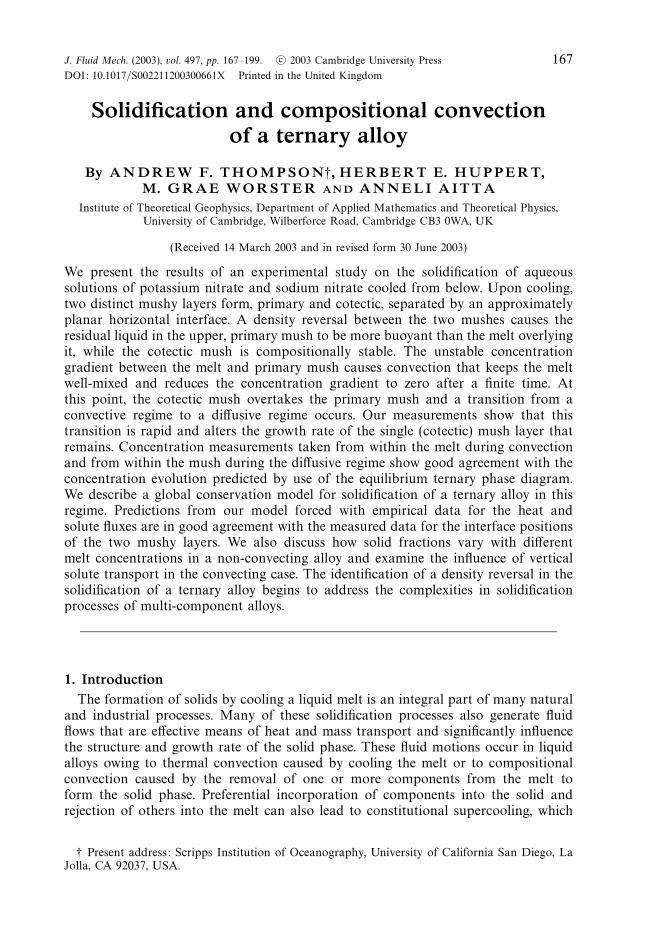
The phase diagram is important because it determines the order in which eachcomponent of an alloy solidifies along the liquid line of descent. A plan view of asimple ternary phase diagram with a single ternary eutectic point and a typical liquidline of descent is shown in figure 1. A ternary alloy initially in a liquid phase cools untilit reaches the liquidus point. The liquidus point lies on the concentration–temperaturesurface, where a single component first begins to solidify. The first component forms asolid crystal matrix bathed in residual liquid in a region called the primary mush. Animportant property of mushy layers is that to a good approximation they conform tolocal thermodynamic equilibrium so that temperature and concentration are coupledby a single relationship (Worster 2000). Within this mushy layer, the residual liquidbecomes enriched in the other two components which remain in the same ratio.This evolution of concentration and the associated temperature in the residual liquidoccurs along the tie line, which connects the liquidus point to the corner of thephase diagram representing the pure solidifying component and intersects one ofthree cotectic curves indicated by the dashed lines in figure 1. These cotectic curvesrepresent the range of concentration and temperature at which two components arein a solid phase coexisting in equilibrium with one another and the remaining liquid.Further cooling leads to the formation of a cotectic mush, which has a crystal matrixof two solid components bathed in residual liquid, and causes the concentrationand temperature of the residual liquid to evolve along the cotectic curve. Eventuallythe system will reach its eutectic point, the only combination of concentration andtemperature at which all three solid components and a liquid phase can co-exist inequilibrium. Cooling below the eutectic point leads to the formation of a eutecticcomposite solid.
Aitta, Huppert & Worster (2001b, herein referred to as AHW) initiated anexperimental study of ternary alloys in a laboratory setting by cooling from belowa simple alloy of two salts dissolved in water. Temperature and concentrationmeasurements were made at different heights within the tank and at various times,and the positions of the melt–mush interface and the mush–solid interface weretracked over time. In that study, the initial concentrations of the alloy were chosen
Solidification and compositional convection of a ternary alloy 169
A C
B
Liquiduspoint
Cotecticpoint Ternary
eutectic point
Figure 1. Plan view of a simple ternary phase diagram depicting a typical liquid line ofdescent. In this diagram, the three fields are separated by the cotectic curves (dashed lines)and temperature is measured along the vertical axis out of the page. Here the liquidus pointfalls in the field associated with B, indicating that it is component B that forms a solid phasein the primary mush. The liquid line of descent (bold line) shows that the temperature andconcentration evolve along the tie line until it reaches the cotectic point. At this point acotectic mush forms composed of solid A and B and residual liquid. Further cooling causesthe temperature and concentration of the residual liquid in the cotectic mush to evolve alongthe cotectic curve until the residual liquid reaches eutectic concentrations. Cooling below theeutectic temperature at these concentrations leads to the formation of a eutectic compositesolid. Similar liquid lines of descent occur in each of the three fields, but the stratificationof the residual liquid in these mushy layers will differ depending on which components areincorporated into a solid phase.
so that the residual liquid in the mushy layers was denser than the fluid overlyingit. The compositional and thermal fields of the alloy were stably stratified at alltimes, and convection did not play a role in the growth dynamics. Results fromthese experiments showed that the growth of the mushy layers and the compositesolid were diffusion-limited and the interface positions of these layers grew at a rateproportional to the square root of time after some initial transients, possibly relatedto a nucleation delay. The interface between the primary and cotectic mushes wasalso inferred through concentration measurements within the mushy layers. In ourexperiments this boundary was measured explicitly through visual observations.
More recently Bloomfield & Huppert (2003) analysed two regimes of an aqueousternary alloy cooled from the side. In the first regime, heavy fluid was releasedupon solidification and both the thermal and compositional boundary layers flowedto the base of the tank. In the second regime, the residual liquid was relativelylight and the thermal and compositional boundary layers were opposed. A widerange of convective behaviours was observable in this case, including uni-directional
170 A. F. Thompson, H. E. Huppert, M. G. Worster and A. Aitta
downflow, counterflow and mixed upflow. Density reversals were also observed, sothat over time the rejected fluid evolved from relatively light to relatively heavy andeventually the dynamics of the first regime were recovered. Our experimental studyinvestigated the solidification of an aqueous ternary alloy from a lower horizontalboundary which incorporated both compositional convection and a density reversal.This density reversal was transient, however, since the layer of light fluid mixed withthe melt above it and eventually disappeared. At this point, as in Bloomfield &Huppert (2003), the dynamics reverted to a simpler case, namely the diffusion-limitedgrowth studied by AHW.
We begin by describing a series of experiments exploring a compositionally unstableregime of a ternary alloy and presenting our observations and results. In § 3 wedevelop a simple global conservation model to describe the experiments. The globalconservation model is an extension of the binary model developed by Huppert &Worster (1985) and modified to include convection by Kerr et al. (1990a). In § 4 weconsider the special case in which convection is absent and investigate the effects ofvarying initial concentrations and the base temperature on the solid fractions. Wediscuss the full model including convection in § 5, and describe how the interfacepositions of the two mushy layers and the solid fractions evolve with time. In thatsection we also compare the positions of the two mushy layers with the experimentalobservations, and discuss a correction term to take into account the heat flux betweenthe laboratory and the experimental tank. We summarize our main results andconclusions in § 6.
2. Laboratory experiments2.1. Methods
The aim of our laboratory experiments was to explore the behaviour of a ternaryalloy cooled from below in a regime where compositional convection affects thesolidification process. We used the ternary alloy selected by AHW consisting oftwo salts, potassium nitrate (KNO3) and sodium nitrate (NaNO3), dissolved in thethird component, water. This alloy was chosen because it is transparent, whichenables visual observation, and because the liquidus and eutectic temperatures couldbe readily reached with typical laboratory equipment. This alloy also conforms to asimple phase diagram without any peritectic points near the ternary eutectic point, andthe concentration of KNO3 and NaNO3 in water could be accurately measured usinga Varian SpectrAA flame atomic absorption spectrometer (AAS). The solidificationfield of interest for the current set of experiments was the KNO3 field. With theconditions explored in the experiments, KNO3 solidified in the primary mush andKNO3 and H2O solidified in the cotectic mush. The liquidus surface was assumed tobe planar (an approximation that will be discussed further in the following section)and the points defining this surface appear in table 1.
The experiments were conducted in a rectangular Perspex tank with internalhorizontal dimensions 20 cm × 20 cm, which was filled with solution to a depth ofapproximately 35 cm. The walls were 1.3 cm thick and the top was covered with aPerspex lid 1.5 cm thick. The base consisted of a 2.5 cm thick brass plate that hadbeen milled to allow coolant to flow through it and cool the plate evenly. The wholesystem was then insulated with a layer of expanded polystyrene whose thickness was5 cm around the sidewalls and above the lid and 10 cm below the baseplate. Theinitial concentrations were decided upon before each experiment and commercialsalts with less than 2% impurities (as stated on the packaging) were measured out
Solidification and compositional convection of a ternary alloy 171
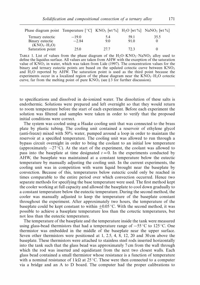
Phase diagram point Temperature [ ◦C] KNO3 [wt %] H2O [wt %] NaNO3 [wt %]
Ternary eutectic −19.0 5.4 59.1 35.5Binary eutectic −2.84 9.0 91.0 0
(KNO3–H2O)Saturation point 25.0 27.7 72.3 0
Table 1. List of values from the phase diagram of the H2O–KNO3–NaNO3 alloy used todefine the liquidus surface. All values are taken from AHW with the exception of the saturationvalue of KNO3 in water, which was taken from Lide (1997). The concentration values for thebinary and ternary eutectic points are based on the updated cotectic curve between KNO3
and H2O reported by AHW. The saturation point is used as the third point because theexperiments occur in a localized region of the phase diagram near the KNO3–H2O cotecticcurve, far from the melting point of pure KNO3 (see § 3 for further discussion).
to specifications and dissolved in de-ionized water. The dissolution of these salts isendothermic. Solutions were prepared and left overnight so that they would returnto room temperature before the start of each experiment. Before each experiment thesolution was filtered and samples were taken in order to verify that the proposedinitial conditions were correct.
The system was cooled using a Haake cooling unit that was connected to the brassplate by plastic tubing. The cooling unit contained a reservoir of ethylene glycol(anti-freeze) mixed with 50% water, pumped around a loop in order to maintain thereservoir at a specified temperature. The cooling unit was allowed to run through abypass circuit overnight in order to bring the coolant to an initial low temperature(approximately −27 ◦C). At the start of the experiment, the coolant was allowed topass into the baseplate at time designated t = 0. In the experiments conducted byAHW, the baseplate was maintained at a constant temperature below the eutectictemperature by manually adjusting the cooling unit. In the current experiments, thecooling unit was in competition with warm liquid brought near the baseplate byconvection. Because of this, temperatures below eutectic could only be reached intimes comparable to the entire period over which convection occurred. Hence twoseparate methods for specifying the base temperature were used. The first method keptthe cooler working at full capacity and allowed the baseplate to cool down gradually toa constant temperature below the eutectic temperature. During the second method, thecooler was manually adjusted to keep the temperature of the baseplate constantthroughout the experiment. After approximately two hours, the temperature of thebaseplate could be kept constant to within ±0.05 ◦C. With the second method, it waspossible to achieve a baseplate temperature less than the cotectic temperatures, butnot less than the eutectic temperature.
The temperature of the baseplate and the temperature inside the tank were measuredusing glass-bead thermistors that had a temperature range of −55 ◦C to 125 ◦C. Onethermistor was embedded in the middle of the baseplate near the upper surface.Seven other thermistors were positioned at 1, 2.5, 4, 8, 12, 20 and 30 cm above thebaseplate. These thermistors were attached to stainless steel rods inserted horizontallyinto the tank such that the glass bead was approximately 7 cm from the wall throughwhich the rod was inserted and equidistant from the next two closest walls. Eachglass bead contained a small thermistor whose resistance is a function of temperaturewith a nominal resistance of 1 k� at 25 ◦C. These were then connected to a computervia a bridge and an A to D board. The computer had the proper calibrations to
172 A. F. Thompson, H. E. Huppert, M. G. Worster and A. Aitta
compute the temperature from the resistances. The computer recorded temperatureautomatically at specified intervals, which could be adjusted during the course of theexperiment.
Samples of the liquid were removed at various times and at various heights using along thin syringe inserted in a small opening at the top of the tank. While the systemwas convecting, the mushy layers were flush against the sides of the tank so sampleswere only removed from the liquid region above the mushy layers. As will be discussedin § 2.2, convection eventually stopped, and the mushy layer formed a humped shapethat allowed samples to be removed from the side of the tank below the melt–mushinterface. To remove samples from this region, the lid of the tank had to be removed.This sampling lasted no longer than one or two minutes. Each sample was thendiluted 1:500 by volume so that accurate readings could be obtained using the AAS.A set of samples with known concentrations for each salt were used as standardsto calibrate the AAS. The AAS used flame emission to determine the concentrationof a given element in water (potassium K and sodium Na for these experiments),given in units of µg cm−3. The calibration, which was highly dependent on thestrength and stability of the flame, was checked after every ten samples. The con-centrations were then converted to a volume percentage by multiplying by the dilutionfactor 500, a factor of 106 (to convert from µg cm−3 to g cm−3), and the molecularweight of the salt divided by the atomic weight of the element. Then the weightpercent was determined by dividing by the density of the liquid. The density wasdetermined using the function,
ρ = 1 + a1N + b1K + a2N2 + b2K
2 + cNK, (2.1)
where N and K are weight percentages of the salts NaNO3 and KNO3 respectively.The values of the coefficients in (2.1) are a1 = 0.006387, a2 = −6.728 × 10⁻⁶, b1 =0.005898, b2 = −2.227 × 10⁻⁶, and c = 2.083 × 10⁻⁴ as given in AHW. By using thestandard solutions, it was determined that the AAS provided accurate concentrationreadings to within ±0.2 wt %.
Other measurements were made by simple observational techniques. The heightof the primary and cotectic mushes and the eutectic solid were measured using aruler and looking through the side of the tank. The interface between the liquid andprimary mush was well-defined at all times. The interface between the primary andcotectic mushes could be distinguished throughout most of the experiment to within±1mm by shining a strong, focused LED penlight through the side of the tank. Thisinterface became more difficult to observe close to the transition from a convectiveto diffusion-controlled regime. In experiments where a eutectic solid formed, the solidlayer was bright white, and the interface between the solid, eutectic layer and thecotectic mushy layer was well-defined. The strength and structure of the convectionwas visualized with standard shadowgraph techniques using a projector and tracingpaper.
2.2. Observations
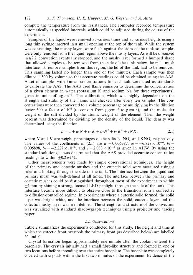
Table 2 summarizes the experiments conducted for this study. The height and time atwhich the cotectic front overtook the primary front (as described below) are labelledh∗ and t∗.
Crystal formation began approximately one minute after the coolant entered thebaseplate. The crystals initially had a small fibre-like structure and formed in one ortwo locations before spreading over the entire baseplate. The baseplate was completelycovered with crystals within the first two minutes of the experiment. Evidence of the
Solidification and compositional convection of a ternary alloy 173
Initial conc.[wt %] Minimum Total
Base base temp. Eutectic duration t∗ h∗
Expt H2O NaNO3 condition [◦C] solid [h] [h] [cm]
1 78 10 constant −17.2 no 58 7.5 2.32 78 10 cooled −27.2 yes 46 6.5 2.53 75.9 9.1 cooled −23.6 yes 71 10 3.44 76.8 3.0 cooled −25.8 no 100 19 4.85 75.9 9.7 cooled −25.7 yes 96 16 3.56 78.0 7.2 cooled −25.7 yes 76 16 4.07 72.6 15.0 constant −14.0 no 105 30 3.38 75 7 constant −14.8 no 105 35 4.4
Table 2. Experimental parameters. The base condition refers to the specification of temperatureat the baseplate, either gradually cooled below the eutectic temperature or maintained at aconstant temperature throughout the experiment; t∗ and h∗ are respectively the time and heightat which the cotectic mush overtook the primary mush; t∗ is also the duration of convectionin each experiment.
development of strong convection was visible within five minutes of the start of theexperiment. This initial convection was sufficiently strong to keep the fluid in the tankwell-mixed. In all the experiments, convection appeared to occur initially in the formof salt fingers for approximately ten minutes. The convection then became muchmore vigorous, which lasted for approximately half the period of total convectingtime, after which it began to decay again into fingering convection. There was noevidence of chimneys in the mushy layer during these experiments. This could be dueto what appeared to be wide spacing between crystals in the primary mush layer,which could allow relatively less dense fluid to rise without dissolving a significantnumber of crystals, the typical mechanism for chimney formation (Worster 2000).After 1 to 2 hours, the crystals looked like short hairs and were finer and thinnerthan those that first covered the baseplate. With this change the interface at the topof the primary mush layer became spiky with some crystals protruding above the flatinterface. In experiments where the baseplate was allowed to cool below the eutectictemperature and convection was strong, some of these fine crystals broke off fromthe solid matrix and were carried into the liquid layer by convective fluid motion.Similar observations were made in experiments by Sarazin & Hellawell (1992) wherechimney formation was reported. Unlike the mushy layers in the diffusion-limitedgrowth regime described by AHW, which were hump-shaped with open fluid betweenthe mush and side walls over most of their height, the mush here remained flushagainst the side walls of the tank.
After the first few hours, the top of the cotectic layer began to catch up slowlywith the top of the primary mush layer. After approximately half the convectingtime the crystals still had a hair-like structure, but had become thicker. During thisperiod the convection continued steadily. In the experiments where the baseplatewas continuously cooled, convection started to weaken after approximately 12 to14 hours. In the case where the baseplate was kept at a constant temperature (andat a higher temperature than the other set of experiments), convection started toweaken after approximately 23 hours. The weakening of convection corresponded tothe thinning of the primary mush layer and the establishment of fingering convection,which eventually led to the entire depth of the tank no longer being well-mixed. As
174 A. F. Thompson, H. E. Huppert, M. G. Worster and A. Aitta
the primary mush layer became very thin, the crystal structure at the melt–mushinterface again appeared to change as the hair-like crystals seemed to disappear orbe dissolved. Once the cotectic layer had overtaken the primary mush, convectionceased completely. Shortly after this transition, the crystal structure was replaced by amore solid-looking mush that was corrugated. The process of convection weakeningand then ceasing happened more abruptly in the experiments where the baseplatewas allowed to cool below the eutectic temperature. In general, though, the transitionbetween a convecting state and a diffusion-controlled state was rapid compared tothe length of time during which convection occurred.
At the height where the cotectic mush overtook the primary mush, a visiblehorizontal interface remained behind as the mush continued to grow. This interfacewas identifiable by a change in crystal structure or solid fraction and remained visibleand at a constant height as the experiment progressed. As the mushy layer continuedto grow into the liquid, a space formed between the sides of the tank and the mushylayer. This space, which increased with height and grew to a width of approximately2 cm, was similar to the gap observed by AHW in the diffusion-controlled, non-convecting regime of this alloy. This gap is most likely to have been caused by heatgains from the laboratory.
A eutectic solid layer was observed in four of the experiments where the baseplatewas allowed to cool below the eutectic temperature. It formed well after the baseplatehad been cooled below the eutectic temperature. This is similar to the long nucleationtimes for the eutectic solid observed by AHW. In the experiments where a eutecticsolid formed, the time at which this layer first became visible coincided with the timethat convection ceased completely. Eutectic solid was not observed in one experimentwhere the baseplate temperature was below the eutectic temperature: the initialconcentration of NaNO3 was low in this experiment, and would have had to increaseby an order of magnitude to reach its eutectic concentration. This may have eitherled to longer delays in the nucleation of the solid, or made it difficult for the systemto conform to equilibrium dynamics at low temperatures.
2.3. Measurements
2.3.1. Temperatures
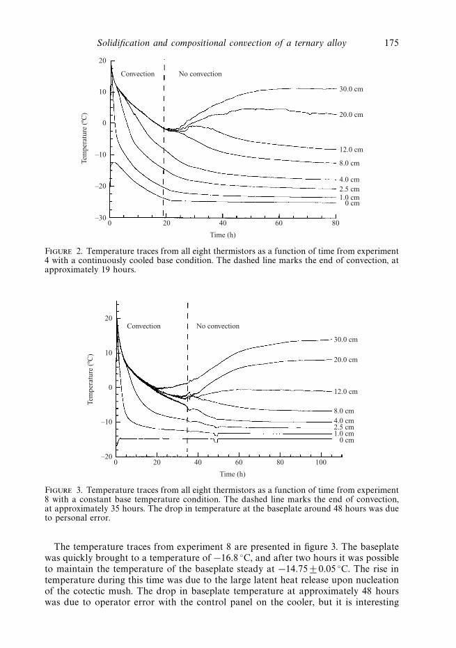
The temperatures measured in experiment 4, with a continuously cooled baseplate,are shown in figure 2 as a function of time. A base temperature of −13 ◦C was achievedafter 20 minutes, at which time it rose abruptly before decreasing again at a slowerrate until convection stopped. This short rise in temperature indicates the nucleationof the cotectic mush, since the liquid must be supercooled before the layer can form.The slow change in baseplate temperature suggests that during convection therewas competition between warm liquid brought close to the baseplate by convectionand the coolant within the baseplate. During convection the temperature in themelt was essentially uniform, indicating that this region was well-mixed. Thermistortraces decreased from this uniform temperature as each thermistor entered the mush.There was also a discontinuity in the gradient of the baseplate temperature in allexperiments in which a eutectic solid layer formed. This occurred as the baseplatereached its minimum temperature, and may have been caused by the release oflatent heat during the nucleation of the eutectic solid as well as by the terminationof convection. After convection ended, the temperature near the top of the tankincreased due to heating from the laboratory, and the temperature profile suggeststhat the tank had become thermally stratified.
Solidification and compositional convection of a ternary alloy 175
0 20 40 60 80
Time (h)
–30
–20
–10
0
10
20
Tem
pera
ture
(ºC
)
0 cm1.0 cm2.5 cm4.0 cm
8.0 cm
12.0 cm
20.0 cm
30.0 cm
Convection No convection
Figure 2. Temperature traces from all eight thermistors as a function of time from experiment4 with a continuously cooled base condition. The dashed line marks the end of convection, atapproximately 19 hours.
0 20 40 60 80
Time (h)
–20
–10
0
10
20
Tem
pera
ture
(ºC
)
0 cm1.0 cm2.5 cm4.0 cm8.0 cm
12.0 cm
20.0 cm
30.0 cm
Convection No convection
100
Figure 3. Temperature traces from all eight thermistors as a function of time from experiment8 with a constant base temperature condition. The dashed line marks the end of convection,at approximately 35 hours. The drop in temperature at the baseplate around 48 hours was dueto personal error.
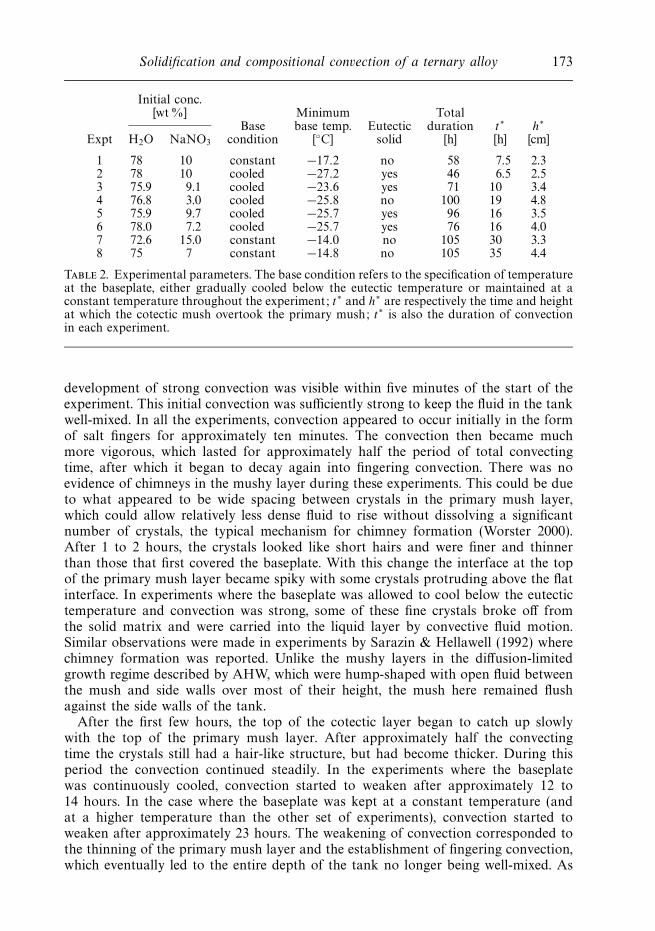
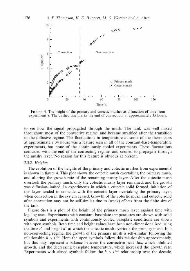
The temperature traces from experiment 8 are presented in figure 3. The baseplatewas quickly brought to a temperature of −16.8 ◦C, and after two hours it was possibleto maintain the temperature of the baseplate steady at −14.75 ± 0.05 ◦C. The rise intemperature during this time was due to the large latent heat release upon nucleationof the cotectic mush. The drop in baseplate temperature at approximately 48 hourswas due to operator error with the control panel on the cooler, but it is interesting
176 A. F. Thompson, H. E. Huppert, M. G. Worster and A. Aitta
0
Time (h)
Hei
ght (
cm) Convection No convection
20 40 60 80 100 120
2
4
6
8
10
Primary mushCotectic mush
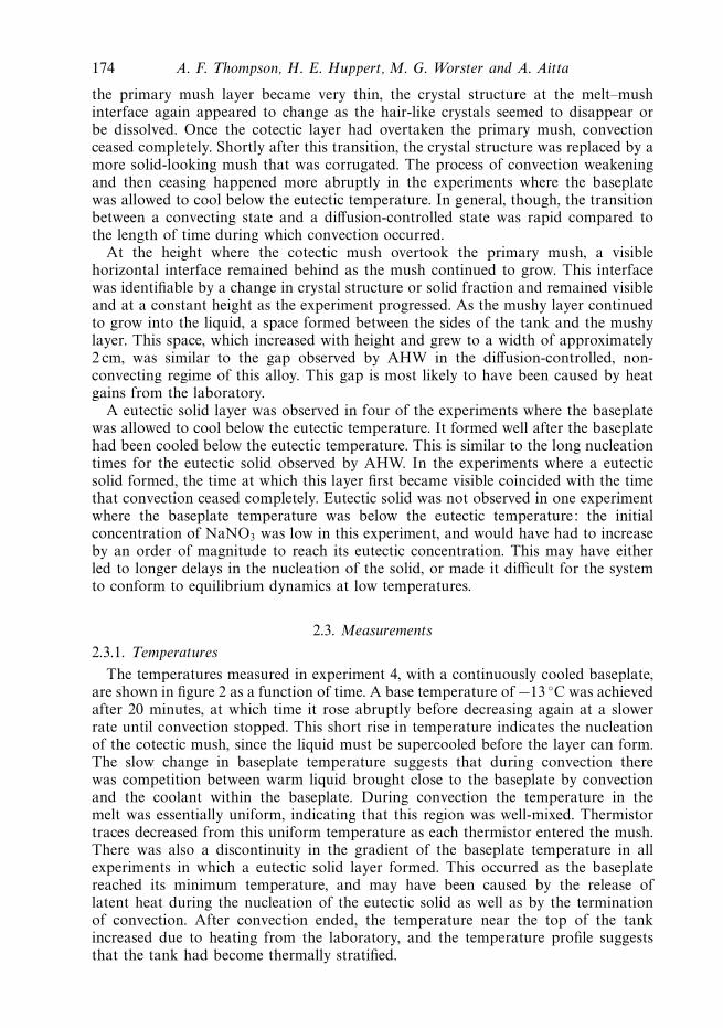
Figure 4. The height of the primary and cotectic mushes as a function of time fromexperiment 8. The dashed line marks the end of convection, at approximately 35 hours.
to see how the signal propagated through the mush. The tank was well mixedthroughout most of the convective regime, and became stratified after the transitionto the diffusive regime. The fluctuations in temperature at some of the thermistorsat approximately 34 hours was a feature seen in all of the constant-base-temperatureexperiments, but none of the continuously cooled experiments. These fluctuationscoincided with the end of the convecting regime, and seemed to propagate throughthe mushy layer. No reason for this feature is obvious at present.
2.3.2. Heights
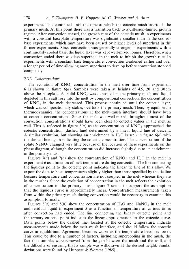
The evolution of the heights of the primary and cotectic mushes from experiment 8is shown in figure 4. This plot shows the cotectic mush overtaking the primary mush,and altering the growth rate of the remaining mushy layer. After the cotectic mushovertook the primary mush, only the cotectic mushy layer remained, and the growthwas diffusion-limited. In experiments in which a eutectic solid formed, initiation ofthis layer tended to coincide with the cotectic layer overtaking the primary layer,when convection in the system ceased. Growth of the cotectic mush and eutectic solidafter convection may not be self-similar due to (weak) effects from the finite size ofthe tank.
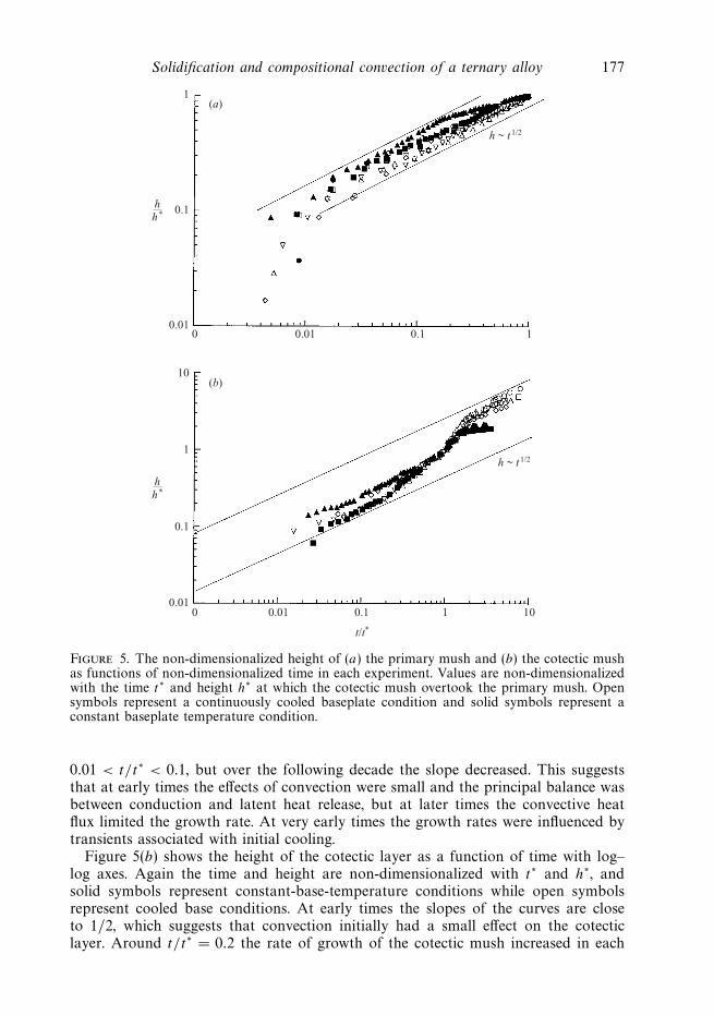
Figure 5(a) is a plot of the height of the primary mush layer against time withlog–log axes. Experiments with constant baseplate temperatures are shown with solidsymbols and experiments with continuously cooled baseplate conditions are shownwith open symbols. Both time and height values have been non-dimensionalized usingthe time t∗ and height h∗ at which the cotectic mush overtook the primary mush. In anon-convecting regime, the growth of the primary mush is self-similar, following therelationship h ∼ t1/2. Here the open symbols follow this relationship approximately,but this may represent a balance between the convective heat flux, which inhibitedgrowth, and the decreasing baseplate temperature, which increased the growth rate.Experiments with closed symbols follow the h ∼ t1/2 relationship over the decade,
Solidification and compositional convection of a ternary alloy 177
0 0.01 0.1 1 10
0 0.01 0.1 10.01
0.01
0.1
1
10
0.1
1
t/t*
h ~ t1/2
h ~ t1/2
(a)
(b)
hh*
hh*
Figure 5. The non-dimensionalized height of (a) the primary mush and (b) the cotectic mushas functions of non-dimensionalized time in each experiment. Values are non-dimensionalizedwith the time t∗ and height h∗ at which the cotectic mush overtook the primary mush. Opensymbols represent a continuously cooled baseplate condition and solid symbols represent aconstant baseplate temperature condition.
0.01 < t/t∗ < 0.1, but over the following decade the slope decreased. This suggeststhat at early times the effects of convection were small and the principal balance wasbetween conduction and latent heat release, but at later times the convective heatflux limited the growth rate. At very early times the growth rates were influenced bytransients associated with initial cooling.
Figure 5(b) shows the height of the cotectic layer as a function of time with log–log axes. Again the time and height are non-dimensionalized with t∗ and h∗, andsolid symbols represent constant-base-temperature conditions while open symbolsrepresent cooled base conditions. At early times the slopes of the curves are closeto 1/2, which suggests that convection initially had a small effect on the cotecticlayer. Around t/t∗ = 0.2 the rate of growth of the cotectic mush increased in each
178 A. F. Thompson, H. E. Huppert, M. G. Worster and A. Aitta
experiment. This continued until the time at which the cotectic mush overtook theprimary mush. At this point there was a transition back to a diffusion-limited growthregime. After convection ceased, the growth rate of the cotectic mush in experimentswith a constant baseplate temperature was significantly smaller than in the cooled-base experiments, which may have been caused by higher levels of superheat in theformer experiments. Since convection was generally stronger in experiments with acontinuously cooled base, the liquid layer was kept well-mixed longer. Therefore, whenconvection ended there was less superheat in the melt to inhibit the growth rate. Inexperiments with a constant base temperature, convection weakened earlier and overa longer period of time allowing more superheat to develop before convection stoppedcompletely.
2.3.3. Concentrations
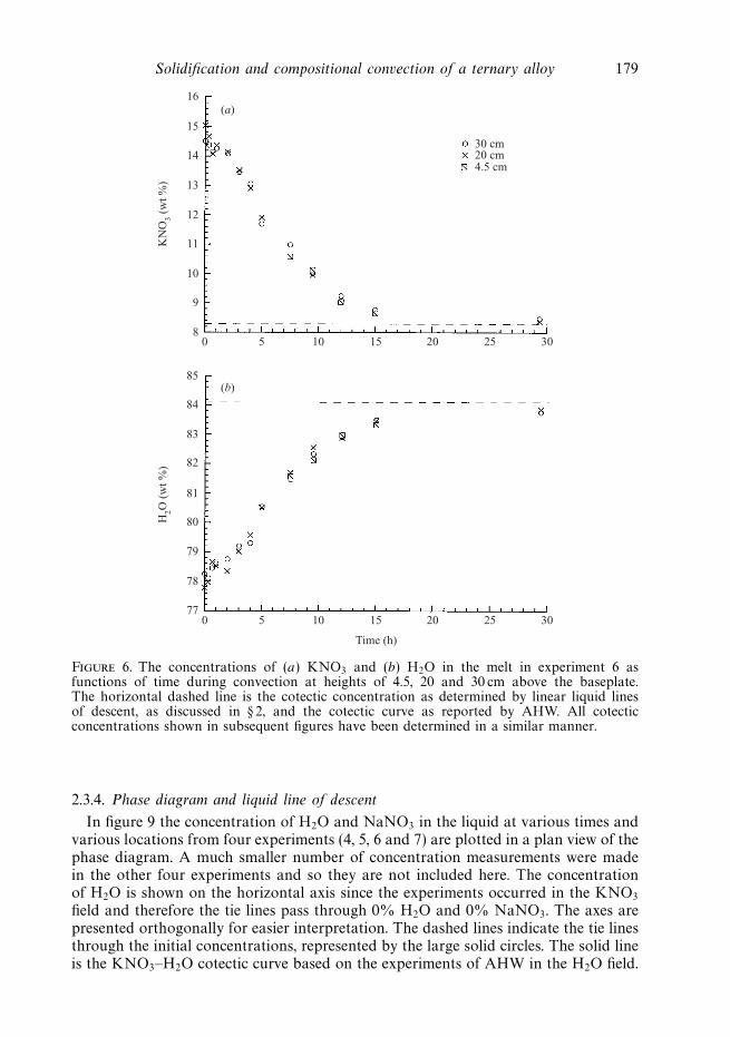
The evolution of KNO3 concentration in the melt over time from experiment6 is shown in figure 6(a). Samples were taken at heights of 4.5, 20 and 30 cmabove the baseplate. As solid KNO3 was deposited in the primary mush and liquiddepleted in this salt rose into the melt by compositional convection, the concentrationof KNO3 in the melt decreased. This process continued until the cotectic layer,which was compositionally stable, overtook the primary mush. Then, by equilibriumthermodynamics, the concentrations at the melt–mush interface should have beenat cotectic concentrations. Since the melt was well-mixed throughout most of theconvection, concentrations should have been close to cotectic values in the melt aswell. This is reflected in figure 6(a) as the concentration of KNO3 approached thecotectic concentration (dashed line) determined by a linear liquid line of descent.A similar evolution, but showing an enrichment in H2O is seen in figure 6(b) withthe dashed line again indicating the cotectic concentration. The concentration of thesolute NaNO3 changed very little because of the location of these experiments on thephase diagram, although the concentration did increase slightly due to its enrichmentin the primary mush.
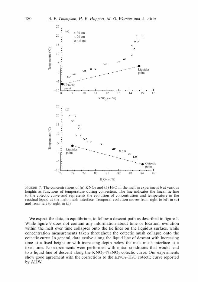
Figures 7(a) and 7(b) show the concentration of KNO3 and H2O in the melt inexperiment 6 as a function of melt temperature during convection. The line connectingthe liquidus point to the cotectic point indicates the linear tie line of this alloy. Weexpect the data to be at temperatures slightly higher than those specified by the tie linebecause temperature and concentration are not coupled in the melt whereas they arein the mushes. Since the evolution of concentration in the melt reflects the evolutionof concentration in the primary mush, figure 7 seems to support the assumptionthat the liquidus curve is approximately linear. Concentration measurements takenfrom within the primary mush during convection would be necessary to examine thisassumption formally.
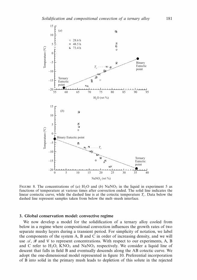
Figures 8(a) and 8(b) show the concentration of H2O and NaNO3 in the meltand residual liquid in experiment 5 as a function of temperature at various timesafter convection had ended. The line connecting the binary eutectic point andthe ternary eutectic point indicates the linear approximation to the cotectic curve.Data points below the dashed line, located at the cotectic temperature, indicatemeasurements made below the melt–mush interface, and should follow the cotecticcurve in equilibrium. Agreement becomes worse as the temperature becomes lower.This could be due to a number of factors, including supercooling in the mush, thefact that samples were removed from the gap between the mush and the wall, andthe difficulty of ensuring that a sample was withdrawn at the desired height. Similardeviations were found by Huppert & Worster (1985).
Solidification and compositional convection of a ternary alloy 179
(a)
0 5 10 15 20 25 308
9
10
11
12
13
14
15
16
30 cm20 cm4.5 cm
KN
O3
(wt %
)H
2O (
wt %
)
0 5 10 15 20 25 30
Time (h)
77
78
79
80
81
82
83
84
85(b)
Figure 6. The concentrations of (a) KNO3 and (b) H2O in the melt in experiment 6 asfunctions of time during convection at heights of 4.5, 20 and 30 cm above the baseplate.The horizontal dashed line is the cotectic concentration as determined by linear liquid linesof descent, as discussed in § 2, and the cotectic curve as reported by AHW. All cotecticconcentrations shown in subsequent figures have been determined in a similar manner.
2.3.4. Phase diagram and liquid line of descent
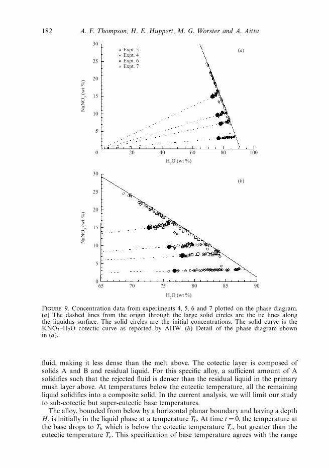
In figure 9 the concentration of H2O and NaNO3 in the liquid at various times andvarious locations from four experiments (4, 5, 6 and 7) are plotted in a plan view of thephase diagram. A much smaller number of concentration measurements were madein the other four experiments and so they are not included here. The concentrationof H2O is shown on the horizontal axis since the experiments occurred in the KNO3
field and therefore the tie lines pass through 0% H2O and 0% NaNO3. The axes arepresented orthogonally for easier interpretation. The dashed lines indicate the tie linesthrough the initial concentrations, represented by the large solid circles. The solid lineis the KNO3–H2O cotectic curve based on the experiments of AHW in the H2O field.
180 A. F. Thompson, H. E. Huppert, M. G. Worster and A. Aitta
(a)
8
30 cm20 cm4.5 cm
Tem
pera
ture
(ºC
)
(b)
9 10 11 12 13 14 15 16–10
–5
0
5
10
15
20
25
KNO3 (wt %)
77 78 79 80 81 82 83 84 85
Tem
pera
ture
(ºC
)
–10
–5
0
5
10
15
20
25
H2O (wt %)
Cotecticpoint
Liquiduspoint
Cotecticpoint
Liquiduspoint
Figure 7. The concentrations of (a) KNO3 and (b) H2O in the melt in experiment 6 at variousheights as functions of temperature during convection. The line indicates the linear tie lineto the cotectic curve and represents the evolution of concentration and temperature in theresidual liquid at the melt–mush interface. Temporal evolution moves from right to left in (a)and from left to right in (b).
We expect the data, in equilibrium, to follow a descent path as described in figure 1.While figure 9 does not contain any information about time or location, evolutionwithin the melt over time collapses onto the tie lines on the liquidus surface, whileconcentration measurements taken throughout the cotectic mush collapse onto thecotectic curve. In general, data evolve along the liquid line of descent with increasingtime at a fixed height or with increasing depth below the melt–mush interface at afixed time. No experiments were performed with initial conditions that would leadto a liquid line of descent along the KNO3–NaNO3 cotectic curve. Our experimentsshow good agreement with the corrections to the KNO3–H2O cotectic curve reportedby AHW.
Solidification and compositional convection of a ternary alloy 181
(a)
Tem
pera
ture
(ºC
)
(b)
NaNO3 (wt %)
H2O (wt %)
55 60 65 70 75 80 85 90 95–20
–15
–10
–5
0
5
10
15
BinaryEutecticpoint
28.6 h48.5 h73.4 h
0 5 10 15 20 25 30 35 40
Binary Eutectic point
Tem
pera
ture
(ºC
)
–20
–15
–10
–5
0
5
10
15
TernaryEutecticpoint
Tc
TernaryEutecticpoint
Tc
Figure 8. The concentrations of (a) H2O and (b) NaNO3 in the liquid in experiment 5 asfunctions of temperature at various times after convection ended. The solid line indicates thelinear contectic curve, while the dashed line is at the cotectic temperature Tc . Data below thedashed line represent samples taken from below the melt–mush interface.
3. Global conservation model: convective regimeWe now develop a model for the solidification of a ternary alloy cooled from
below in a regime where compositional convection influences the growth rates of twoseparate mushy layers during a transient period. For simplicity of notation, we labelthe components of the system A, B and C in order of increasing density, and we willuse A, B and C to represent concentrations. With respect to our experiments, A, Band C refer to H2O, KNO3 and NaNO3 respectively. We consider a liquid line ofdescent that falls in field B and eventually descends along the AB cotectic curve. Weadopt the one-dimensional model represented in figure 10. Preferential incorporationof B into solid in the primary mush leads to depletion of this solute in the rejected
182 A. F. Thompson, H. E. Huppert, M. G. Worster and A. Aitta
(a)
NaN
O3
(wt %
)
H2O (wt %)
0 20 40 60 80 100
5
10
15
20
25
30Expt. 5Expt. 4Expt. 6Expt. 7
(b)
65 70 75 80 85 900
5
10
15
20
25
30
NaN
O3
(wt %
)
H2O (wt %)
Figure 9. Concentration data from experiments 4, 5, 6 and 7 plotted on the phase diagram.(a) The dashed lines from the origin through the large solid circles are the tie lines alongthe liquidus surface. The solid circles are the initial concentrations. The solid curve is theKNO3–H2O cotectic curve as reported by AHW. (b) Detail of the phase diagram shownin (a).
fluid, making it less dense than the melt above. The cotectic layer is composed ofsolids A and B and residual liquid. For this specific alloy, a sufficient amount of Asolidifies such that the rejected fluid is denser than the residual liquid in the primarymush layer above. At temperatures below the eutectic temperature, all the remainingliquid solidifies into a composite solid. In the current analysis, we will limit our studyto sub-cotectic but super-eutectic base temperatures.
The alloy, bounded from below by a horizontal planar boundary and having a depthH , is initially in the liquid phase at a temperature T0. At time t =0, the temperature atthe base drops to Tb which is below the cotectic temperature Tc, but greater than theeutectic temperature Te. This specification of base temperature agrees with the range
Solidification and compositional convection of a ternary alloy 183
Tb
Tp, �0
Tc, �c
� � Tlz = H
z = hp(t)
z = hc(t)
z = 0
Melt(well-mixed)
PrimarymushB
AB
Cotecticmush
�
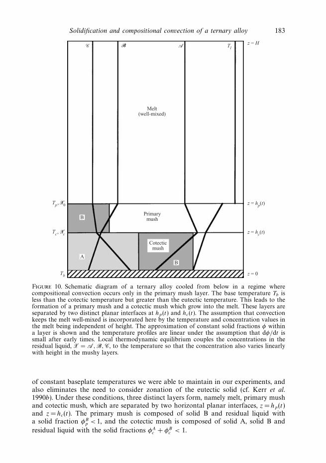
Figure 10. Schematic diagram of a ternary alloy cooled from below in a regime wherecompositional convection occurs only in the primary mush layer. The base temperature Tb isless than the cotectic temperature but greater than the eutectic temperature. This leads to theformation of a primary mush and a cotectic mush which grow into the melt. These layers areseparated by two distinct planar interfaces at hp(t) and hc(t). The assumption that convectionkeeps the melt well-mixed is incorporated here by the temperature and concentration values inthe melt being independent of height. The approximation of constant solid fractions φ withina layer is shown and the temperature profiles are linear under the assumption that dφ/dt issmall after early times. Local thermodynamic equilibrium couples the concentrations in theresidual liquid, X = A, B, C, to the temperature so that the concentration also varies linearlywith height in the mushy layers.
of constant baseplate temperatures we were able to maintain in our experiments, andalso eliminates the need to consider zonation of the eutectic solid (cf. Kerr et al.1990b). Under these conditions, three distinct layers form, namely melt, primary mushand cotectic mush, which are separated by two horizontal planar interfaces, z = hp(t)and z =hc(t). The primary mush is composed of solid B and residual liquid witha solid fraction φB
p < 1, and the cotectic mush is composed of solid A, solid B and
residual liquid with the solid fractions φAc + φB
c < 1.
184 A. F. Thompson, H. E. Huppert, M. G. Worster and A. Aitta
The global conservation model described here is based on the model introduced byHuppert & Worster (1985) for a binary alloy. Our model is also similar to the globalconservation model for diffusion-controlled growth of a ternary alloy described byThompson, Huppert & Worster (2003) with the important addition that the currentmodel allows for convection and time-dependent solid fractions. The model beginswith exact equations for the conservation of heat and solute in each layer, and thenapplies a simplifying assumption about the shape of the solid fraction in these layers.In the model we allow the solid fractions to represent depth-averaged values at everytime step, and therefore they are independent of height.
The model also assumes that local thermodynamic equilibrium holds throughoutthe mushy layers and that temperature and solute concentrations conform to theliquidus relationships. We further assume that a displaced parcel of fluid conformsto the liquidus relationships on time scales that are much shorter than the solutaldiffusive time scale. Therefore equilibrium processes dominate in the mushy layerand the effects of solutal diffusivity can be neglected in this region. We assumethat the difference in concentration across the primary mush drives convection andthat convection keeps the melt well-mixed at all times. The experiments supportthis assumption as the transition from a convective to a diffusion-limited state wasrapid. For simplicity we only consider the effect of the concentration gradient ofcomponent B on the stability of the system. Although depletion of component Band enrichment of component C in the primary mush have opposite effects on thestability of the residual liquid, the concentration gradient of C is small comparedto that of B for the H2O–KNO3–NaNO3 alloy. As the difference in concentrationbetween the melt and primary mush becomes small the stabilizing effect of thetemperature field will become important, and may explain why we observed convectionstopping slightly before the melt reached cotectic concentrations in some of ourexperiments.
Another common assumption is to approximate the liquidus surfaces by planarsurfaces and the cotectic curves by straight lines, so that the liquid line of descentfollows a piecewise linear curve. Then, given information about the phase diagram,these assumptions allow the liquidus and cotectic points to be determined from theinitial conditions of the system. Typically, the planar liquidus surfaces are definedby the freezing point of the component that first solidifies, the binary eutectic pointbetween the two solid components found in the cotectic mush, and the ternary eutecticpoint. In our experiments, though, the evolution of the residual liquid followed a liquidline of descent in a region localized around the cotectic curve. Rather than applyingthe freezing point of component B, which would introduce needless error, we use apoint on the AB binary liquidus curve that is specified by the saturation data forcomponents A and B. The three points of interest are then the saturation point (Asat,C = 0, Tsat), the binary eutectic point of A and B (Abe, C = 0, Tbe), and the ternaryeutectic point (Ae, Ce, Te). We choose to use the concentrations of component A andC in determining the liquidus relationships since the tie line passes through the cornerof pure B on the phase diagram, or 0 wt % A and C, which we take as our origin (cf.figure 9). Then the liquidus temperature Tp and the cotectic temperature Tc are givenby
Tp = Tsat − m(A0 − Asat) − nC0, (3.1)
Tc =Te + mc[(Tsat + mAsat)/mp − Ae]
1 + mc/mp
, (3.2)
Solidification and compositional convection of a ternary alloy 185
where A0 and C0 are the initial concentrations and m, n, mp and mc are the followingslopes on the phase diagram:
m =Tsat − Tbe
Abe − Asat
, (3.3)
n =Tsat − Te − m(Ae − Asat)
Ce
, (3.4)
mp = m +C0
A0
n, (3.5)
mc =Tbe − Te
Abe − Ae
. (3.6)
The concentrations at the cotectic point Ac and Cc can be found using equation (3.1)by replacing Tp with Tc and using the fact that Ac = (A0/C0)Cc at the cotectic point.
3.1. Model with empirical fluxes
Each of the three layers in this model is considered as a continuum with a separateset of equations governing the dynamics in that region. Boundary conditions areprovided at the interfaces between the different layers using the liquidus relationships,and the growth rates are coupled by conservation of heat at the interfaces. Unlike thediffusion-limited case, solute can be transported vertically due to convection, whichmodifies our equations for solute conservation. In the following analysis, subscripts l,p and c stand for the melt, primary mush and cotectic mush respectively.
In the melt, H > z > hp(t), convection keeps the liquid well-mixed so that
T = Tl(t) (3.7)
X = Xl(t), X = B, C, (3.8)
and we assume that these concentrations are equal to their values at the melt–mushinterface. The convective heat flux FT and the solute flux FC between the melt and themush can then be determined from the evolution of temperature and concentrationin the melt. We include a discussion of the relationship between FT and FC below,but in our simulations we applied empirical data from the melt and calculated thefluxes from the relationships
FC = −(H − hp)dBl
dt, (3.9)
FT = −ρCp(H − hp)dTl
dt, (3.10)
where a positive value of FC or FT represents a flux from the melt into the primarymush. Again we note that our assumption of convection being driven solely by theconcentration gradient in component B might not be valid for all alloys. Rejection ofsolute C would tend to reduce the value of both FC and FT .
In the global conservation models of diffusion-controlled solidifying alloys, the solidfractions are independent of time. Then applying the quasi-stationary approximation(linear temperature profile), latent heat is only released at the interfaces as themushy layers grow vertically. If the depth-averaged solid fractions are dependenton time, though, there can also be a release of latent heat within the mushy layerdue to changes in the solid fraction. Kerr et al. (1990a) show that when the globalconservation model is applied to a solidification problem where the solid fractions φ
are assumed uniform but vary with time, the temperature profile is quadratic. This
186 A. F. Thompson, H. E. Huppert, M. G. Worster and A. Aitta
temperature profile modifies the Stefan condition by introducing a new term thataccounts for the latent heat release within the mush. The Stefan condition at themelt–mush interface, z = hp(t), becomes
[ρCp(Tl − Tp) + φB
p ρBLB
] dhp
dt+
1
2ρBLB(hp − hc)
dφBp
dt= kp
(Tp − Tc)
(hp − hc)− FT , (3.11)
where ρ and Cp are the density and specific heat of the melt, ρB and LB are the density
and the latent heat release of solid B and kp is the average thermal conductivity ofthe primary mush, given by
kp = φBp kB +
(1 − φB
p
)kl (3.12)
as discussed by Batchelor (1974). We will assume that the effect of the quadratic termis small since dφ/dt is only significant when the height of the mushy layers are verysmall. Therefore we can continue to use the approximation that temperature varieslinearly with height in the mushy layers.
Conservation of solute B in the primary mush is expressed by∫ hp
hc
[(1 − φB
p
)B + φB
p
ρB
ρl
Bs
]dz = Bp(t)(hp(t) − hc(t)), (3.13)
in which we include the effects of a change in density between the liquid andsolid phase but assume that the depth of the alloy H remains constant since H �hp . Here Bs represents the concentration of solid B and is equal to 100 wt % if
solid immiscibility is assumed, and Bp represents the bulk concentration of soluteB in the primary mush. In the diffusion-limited regime the bulk concentration isconstant, but here it changes with time due to vertical solute transport. At thispoint we apply our approximations that the solid fraction is independent of heightand, as discussed above, that the temperature profile is approximately linear. Localthermodynamic equilibrium and a piecewise linear liquid line of descent then prescribethat concentration must also vary linearly with height in the mushy layers, and wecan modify (3.13) to obtain
Bp = 12
(1 − φB
p
)(Bl + Bc) + φB
p (ρB/ρl)Bs, (3.14)
where Bl and Bc are the concentrations at the upper and lower interfaces of theprimary mush. The bulk concentration of solute B in the primary mush changes dueto the growth of this layer into the melt and a deposition of salt caused by the soluteflux. The growth of the cotectic mush into the primary mush does not alter the bulkconcentration in the primary mush. This relationship can be written as
(hp − hc)dBp
dt= (Bl − Bp)
dhp
dt+ FC. (3.15)
At the interface between the primary and cotectic mushes, z =hc(t), the Stefancondition becomes
[φA
c ρALA +(φB
c − φBp
)ρBLB
]dhc
dt+
1
2hc
(ρALA
dφAc
dt+ ρBLB
dφBc
dt
)
= kc
(Tc − Tb)
hc
− kp
(Tp − Tc)
(hp − hc), (3.16)
where the averaged thermal conductivity in the cotectic mush is
kc = φAc kA + φB
c kB +(1 − φA
c − φBc
)kl. (3.17)
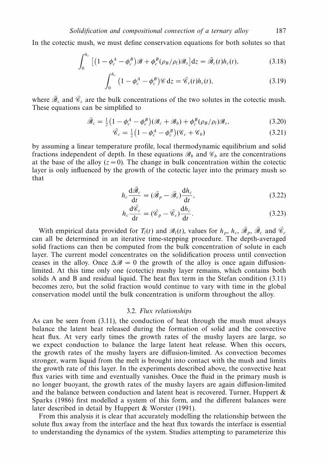
Solidification and compositional convection of a ternary alloy 187
In the cotectic mush, we must define conservation equations for both solutes so that
∫ hc
0
[(1 − φA
c − φBc
)B + φB
c (ρB/ρl)Bs
]dz = Bc(t)hc(t), (3.18)
∫ hc
0
(1 − φA
c − φBc
)C dz = Cc(t)hc(t), (3.19)
where Bc and Cc are the bulk concentrations of the two solutes in the cotectic mush.These equations can be simplified to
Bc = 12
(1 − φA
c − φBc
)(Bc + Bb) + φB
c (ρB/ρl)Bs, (3.20)
Cc = 12
(1 − φA
c − φBc
)(Cc + Cb) (3.21)
by assuming a linear temperature profile, local thermodynamic equilibrium and solidfractions independent of depth. In these equations Bb and Cb are the concentrationsat the base of the alloy (z =0). The change in bulk concentration within the cotecticlayer is only influenced by the growth of the cotectic layer into the primary mush sothat
hc
dBc
dt= (Bp − Bc)
dhc
dt, (3.22)
hc
dCc
dt= (Cp − Cc)
dhc
dt. (3.23)
With empirical data provided for Tl(t) and Bl(t), values for hp , hc, Bp , Bc and Cc
can all be determined in an iterative time-stepping procedure. The depth-averagedsolid fractions can then be computed from the bulk concentration of solute in eachlayer. The current model concentrates on the solidification process until convectionceases in the alloy. Once �B = 0 the growth of the alloy is once again diffusion-limited. At this time only one (cotectic) mushy layer remains, which contains bothsolids A and B and residual liquid. The heat flux term in the Stefan condition (3.11)becomes zero, but the solid fraction would continue to vary with time in the globalconservation model until the bulk concentration is uniform throughout the alloy.
3.2. Flux relationships
As can be seen from (3.11), the conduction of heat through the mush must alwaysbalance the latent heat released during the formation of solid and the convectiveheat flux. At very early times the growth rates of the mushy layers are large, sowe expect conduction to balance the large latent heat release. When this occurs,the growth rates of the mushy layers are diffusion-limited. As convection becomesstronger, warm liquid from the melt is brought into contact with the mush and limitsthe growth rate of this layer. In the experiments described above, the convective heatflux varies with time and eventually vanishes. Once the fluid in the primary mush isno longer buoyant, the growth rates of the mushy layers are again diffusion-limitedand the balance between conduction and latent heat is recovered. Turner, Huppert &Sparks (1986) first modelled a system of this form, and the different balances werelater described in detail by Huppert & Worster (1991).
From this analysis it is clear that accurately modelling the relationship between thesolute flux away from the interface and the heat flux towards the interface is essentialto understanding the dynamics of the system. Studies attempting to parameterize this
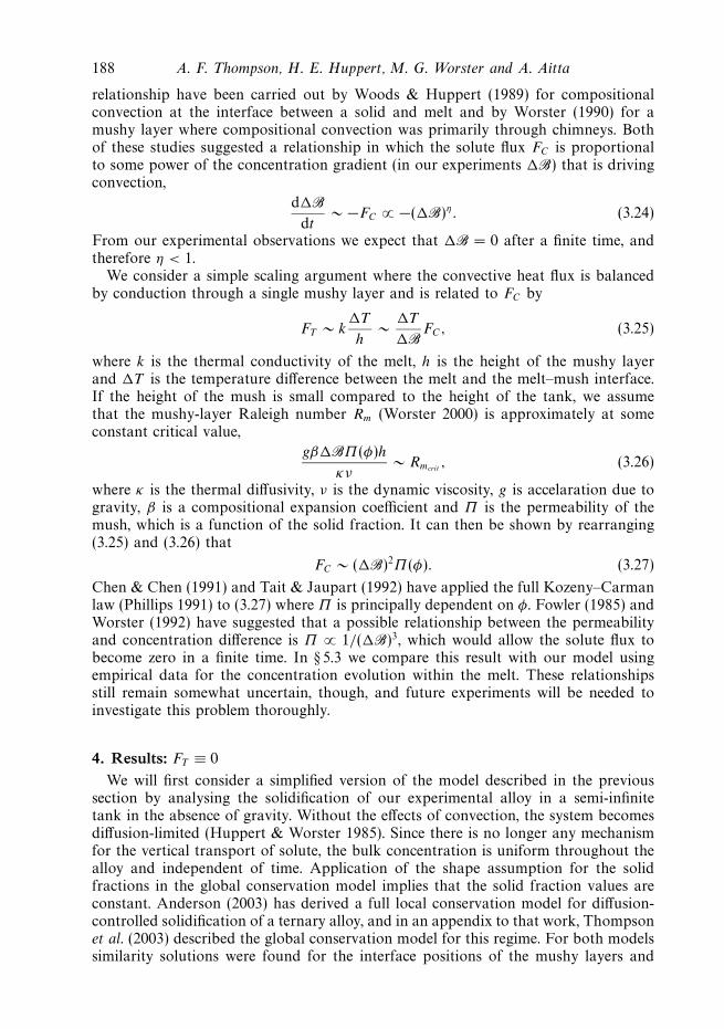
188 A. F. Thompson, H. E. Huppert, M. G. Worster and A. Aitta
relationship have been carried out by Woods & Huppert (1989) for compositionalconvection at the interface between a solid and melt and by Worster (1990) for amushy layer where compositional convection was primarily through chimneys. Bothof these studies suggested a relationship in which the solute flux FC is proportionalto some power of the concentration gradient (in our experiments �B) that is drivingconvection,
d�Bdt
∼ −FC ∝ −(�B)η. (3.24)
From our experimental observations we expect that �B = 0 after a finite time, andtherefore η < 1.
We consider a simple scaling argument where the convective heat flux is balancedby conduction through a single mushy layer and is related to FC by
FT ∼ k�T
h∼ �T
�BFC, (3.25)
where k is the thermal conductivity of the melt, h is the height of the mushy layerand �T is the temperature difference between the melt and the melt–mush interface.If the height of the mush is small compared to the height of the tank, we assumethat the mushy-layer Raleigh number Rm (Worster 2000) is approximately at someconstant critical value,
gβ�BΠ(φ)h
κν∼ Rmcrit
, (3.26)
where κ is the thermal diffusivity, ν is the dynamic viscosity, g is accelaration due togravity, β is a compositional expansion coefficient and Π is the permeability of themush, which is a function of the solid fraction. It can then be shown by rearranging(3.25) and (3.26) that
FC ∼ (�B)2Π(φ). (3.27)
Chen & Chen (1991) and Tait & Jaupart (1992) have applied the full Kozeny–Carmanlaw (Phillips 1991) to (3.27) where Π is principally dependent on φ. Fowler (1985) andWorster (1992) have suggested that a possible relationship between the permeabilityand concentration difference is Π ∝ 1/(�B)3, which would allow the solute flux tobecome zero in a finite time. In § 5.3 we compare this result with our model usingempirical data for the concentration evolution within the melt. These relationshipsstill remain somewhat uncertain, though, and future experiments will be needed toinvestigate this problem thoroughly.
4. Results: FT ≡ 0
We will first consider a simplified version of the model described in the previoussection by analysing the solidification of our experimental alloy in a semi-infinitetank in the absence of gravity. Without the effects of convection, the system becomesdiffusion-limited (Huppert & Worster 1985). Since there is no longer any mechanismfor the vertical transport of solute, the bulk concentration is uniform throughout thealloy and independent of time. Application of the shape assumption for the solidfractions in the global conservation model implies that the solid fraction values areconstant. Anderson (2003) has derived a full local conservation model for diffusion-controlled solidification of a ternary alloy, and in an appendix to that work, Thompsonet al. (2003) described the global conservation model for this regime. For both modelssimilarity solutions were found for the interface positions of the mushy layers and
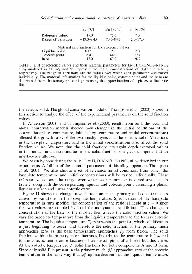
Solidification and compositional convection of a ternary alloy 189
Tb [◦C] A0 [wt %] C0 [wt%]
Reference values −15.0 75.0 7.0Range of variation −19.0–8.45 70.0–84.7 2.0–17.0
Material information for the reference valuesLiquidus point 8.45 75.0 7.0Cotectic point −6.41 84.0 7.84Base −15.0 67.0 26.7
Table 3. List of reference values and their material parameters for the H2O–KNO3–NaNO3
alloy analysed in § 4. A0 and C0 represent the initial concentrations of H2O and KNO3
respectively. The range of variations are the values over which each parameter was variedindividually. The material information for the liquidus point, cotectic point and the base aredetermined from the ternary phase diagram using the approximation of a piecewise linear tieline.
the eutectic solid. The global conservation model of Thompson et al. (2003) is used inthis section to analyse the effect of the experimental parameters on the solid fractionvalues.
In Anderson (2003) and Thompson et al. (2003), results from both the local andglobal conservation models showed how changes in the initial conditions of thesystem (baseplate temperature, initial alloy temperature and initial concentrations)affected the growth rates of the two mushy layers and the eutectic solid. Variationsin the baseplate temperature and in the initial concentrations also affect the solidfraction values. We note that the solid fractions are again depth-averaged valuesin this model, and discontinuities in the solid fraction of a given component at aninterface are allowed.
We begin by considering the A–B–C ≡ H2O–KNO3–NaNO3 alloy described in ourexperiments. A full list of the material parameters of this alloy appears in Thompsonet al. (2003). We also choose a set of reference initial conditions from which thebaseplate temperature and initial concentrations will be varied individually. Thesereference values and the ranges over which each parameter is varied are listed intable 3 along with the corresponding liquidus and cotectic points assuming a planarliquidus surface and linear cotectic curve.
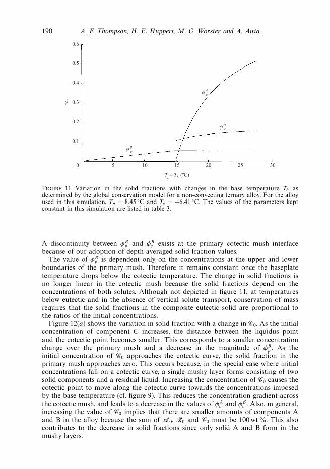
Figure 11 shows the change in solid fractions in the primary and cotectic mushescaused by variations in the baseplate temperature. Specification of the baseplatetemperature in turn specifies the concentration of the residual liquid at z = 0 sincethe two values are coupled by local thermodynamic equilibrium. This change inconcentration at the base of the mushes then affects the solid fraction values. Wevary the baseplate temperature from the liquidus temperature to the ternary eutectictemperature. The liquidus temperature Tp represents the point at which solidificationis just beginning to occur, and therefore the solid fraction of the primary mushapproaches zero as the base temperature approaches Tp from below. The solidfraction within the primary mush increases linearly as the temperature is loweredto the cotectic temperature because of our assumption of a linear liquidus curve.At the cotectic temperature Tc solid fractions for both components A and B form.Since only solid B is present in the primary mush, φA
c approaches zero at the cotectictemperature in the same way that φB
p approaches zero at the liquidus temperature.
190 A. F. Thompson, H. E. Huppert, M. G. Worster and A. Aitta
0 5 10 15 20 25 30
0.1
0.2
0.3
0.4
0.5
0.6
Tp– Tb (ºC)
φ
φBp
φBc
φAc
Figure 11. Variation in the solid fractions with changes in the base temperature Tb asdetermined by the global conservation model for a non-convecting ternary alloy. For the alloyused in this simulation, Tp = 8.45 ◦C and Tc = −6.41 ◦C. The values of the parameters keptconstant in this simulation are listed in table 3.
A discontinuity between φBp and φB
c exists at the primary–cotectic mush interfacebecause of our adoption of depth-averaged solid fraction values.
The value of φBp is dependent only on the concentrations at the upper and lower
boundaries of the primary mush. Therefore it remains constant once the baseplatetemperature drops below the cotectic temperature. The change in solid fractions isno longer linear in the cotectic mush because the solid fractions depend on theconcentrations of both solutes. Although not depicted in figure 11, at temperaturesbelow eutectic and in the absence of vertical solute transport, conservation of massrequires that the solid fractions in the composite eutectic solid are proportional tothe ratios of the initial concentrations.
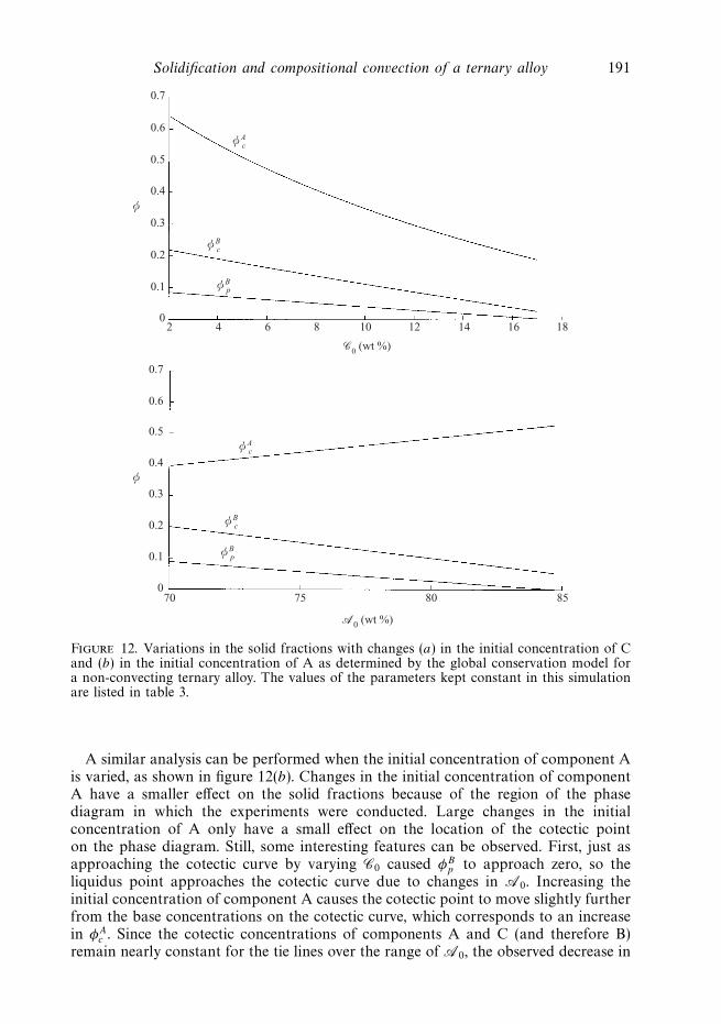
Figure 12(a) shows the variation in solid fraction with a change in C0. As the initialconcentration of component C increases, the distance between the liquidus pointand the cotectic point becomes smaller. This corresponds to a smaller concentrationchange over the primary mush and a decrease in the magnitude of φB
p . As theinitial concentration of C0 approaches the cotectic curve, the solid fraction in theprimary mush approaches zero. This occurs because, in the special case where initialconcentrations fall on a cotectic curve, a single mushy layer forms consisting of twosolid components and a residual liquid. Increasing the concentration of C0 causes thecotectic point to move along the cotectic curve towards the concentrations imposedby the base temperature (cf. figure 9). This reduces the concentration gradient acrossthe cotectic mush, and leads to a decrease in the values of φA
c and φBc . Also, in general,
increasing the value of C0 implies that there are smaller amounts of components Aand B in the alloy because the sum of A0, B0 and C0 must be 100 wt %. This alsocontributes to the decrease in solid fractions since only solid A and B form in themushy layers.
Solidification and compositional convection of a ternary alloy 191
φ
φAc
2 4 6 8 10 12 14 16 180
0.1
0.2
0.3
0.4
0.5
0.6
0.7
φBc
φBp
�0 (wt %)
70 75 80 850
0.1
0.2
0.3
0.4
0.5
0.6
0.7
�0 (wt %)
φ
φAc
φBc
φBp
Figure 12. Variations in the solid fractions with changes (a) in the initial concentration of Cand (b) in the initial concentration of A as determined by the global conservation model fora non-convecting ternary alloy. The values of the parameters kept constant in this simulationare listed in table 3.
A similar analysis can be performed when the initial concentration of component Ais varied, as shown in figure 12(b). Changes in the initial concentration of componentA have a smaller effect on the solid fractions because of the region of the phasediagram in which the experiments were conducted. Large changes in the initialconcentration of A only have a small effect on the location of the cotectic pointon the phase diagram. Still, some interesting features can be observed. First, just asapproaching the cotectic curve by varying C0 caused φB
p to approach zero, so theliquidus point approaches the cotectic curve due to changes in A0. Increasing theinitial concentration of component A causes the cotectic point to move slightly furtherfrom the base concentrations on the cotectic curve, which corresponds to an increasein φA
c . Since the cotectic concentrations of components A and C (and therefore B)remain nearly constant for the tie lines over the range of A0, the observed decrease in
192 A. F. Thompson, H. E. Huppert, M. G. Worster and A. Aitta
φBc with increasing A0 is primarily caused by a reduction in the bulk concentration
of solute B.In the convecting case, the evolution of the melt follows a tie line, which is very
similar to varying A0 as described above (changes in C are small). In the casesdiscussed here, however, each different solid fraction value represents a differentrealization of the simulation where the initial concentration, or solute content, ofthe alloy was changed. With convection, the change in concentration at the upperboundary of the mushy layer will still influence the solid fractions by increasing orreducing the concentration gradient over a layer, but now a more important effect isthat changes in concentration in the melt must be balanced by changes in the solidfractions in the mushy layers in order to conserve solute.
5. Results: full modelWe now consider the full model developed in § 3.1 where the solidification process
takes place in a gravitational field, and buoyancy forces give rise to convection thatsignificantly alters the behaviour of the system. In this model, convection only occurswithin the primary mush and the melt layers due to a compositional instability (thethermal field is stably stratified at all times). In reality this convection may causefluid motion in the cotectic layer as well, but thermistor traces suggest that this flowis very weak. Convection also stops completely after a finite period of time. Whenconvection has ceased the melt–mush interface has concentrations equivalent to thealloy’s cotectic concentrations and therefore only a single mush exists composed oftwo solids and a residual liquid. The analysis in this section concentrates primarilyon the convective regime until the transition to a diffusion-controlled system occurs.
This model provides information about the interface positions hp(t) and hc(t) andthe depth-averaged solid-fraction values φB
p (t), φAc (t) and φB
c (t). The assumptionsdiscussed in § 3.1 still apply. The model uses empirical data for the evolution oftemperature and concentration in the melt, which provides empirical values for thesolute flux and convective heat flux through (3.9) and (3.10).
We initialize the model with small height values for the primary and cotecticmush to avoid the singularity in the Stefan conditions at time t = 0. The heightsare initialized based on the asymptotic limit of a similarity solution for growth ina diffusion-controlled regime. We make this assumption because at early times thegrowth rate is large and the principal balance is between conduction and latentheat release (Huppert & Worster 1991). Temperature and concentration values arealso initialized at the two interfaces and at z = 0 based on the initial conditionsB0, C0, T0 and Tb and the corresponding liquid line of descent. We consider caseswhere Tc > Tb > Te and Tb is a constant. This model can also be easily modifiedto include empirical values for Tb in experiments where the baseplate temperaturewas not held constant. At the first time step, the concentration of component B(KNO3) and temperature in the melt are updated which determines the solute andconvective heat fluxes respectively. The heights of the two mushy layers are thenupdated simultaneously using the Stefan condition at each interface, (3.11) and (3.16),by applying a second-order Runge–Kutta scheme. The updated heights are usedto determine the change in solute bulk concentrations in both mushy layers fromequations (3.15), (3.22) and (3.23). Finally, the new depth-averaged values of the threesolid fractions are determined using (3.14), (3.20) and (3.21). The model continuesthese iterations until the height of the cotectic mush is just greater than the primarymush, which indicates that convection has stopped. In this model we assume that the
Solidification and compositional convection of a ternary alloy 193
0 5 10 15 20 25 30
1
2
3
4
5
6
7
8Primary mush (experimental)
Cotectic mush (experimental)Model without lab heat fluxModel with lab heat flux
Time (h)
Hei
ght (
cm)
Cotectic
Primary
Primary
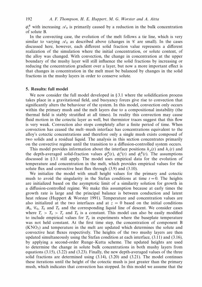
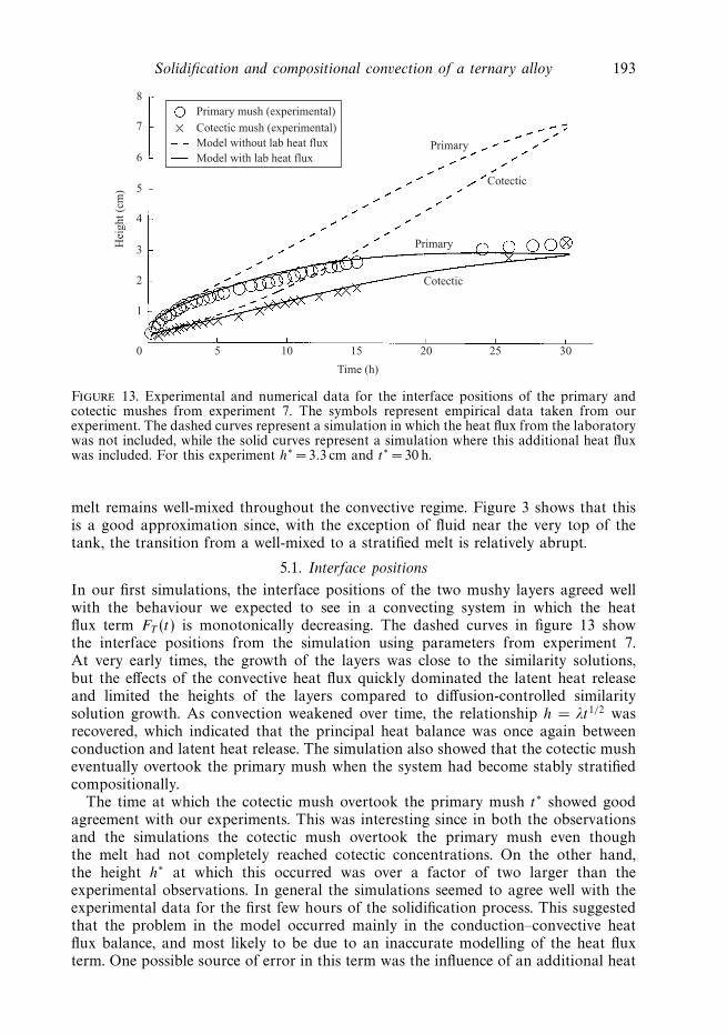
Cotectic
Figure 13. Experimental and numerical data for the interface positions of the primary andcotectic mushes from experiment 7. The symbols represent empirical data taken from ourexperiment. The dashed curves represent a simulation in which the heat flux from the laboratorywas not included, while the solid curves represent a simulation where this additional heat fluxwas included. For this experiment h∗ = 3.3 cm and t∗ = 30 h.
melt remains well-mixed throughout the convective regime. Figure 3 shows that thisis a good approximation since, with the exception of fluid near the very top of thetank, the transition from a well-mixed to a stratified melt is relatively abrupt.
5.1. Interface positions
In our first simulations, the interface positions of the two mushy layers agreed wellwith the behaviour we expected to see in a convecting system in which the heatflux term FT (t) is monotonically decreasing. The dashed curves in figure 13 showthe interface positions from the simulation using parameters from experiment 7.At very early times, the growth of the layers was close to the similarity solutions,but the effects of the convective heat flux quickly dominated the latent heat releaseand limited the heights of the layers compared to diffusion-controlled similaritysolution growth. As convection weakened over time, the relationship h = λt1/2 wasrecovered, which indicated that the principal heat balance was once again betweenconduction and latent heat release. The simulation also showed that the cotectic musheventually overtook the primary mush when the system had become stably stratifiedcompositionally.
The time at which the cotectic mush overtook the primary mush t∗ showed goodagreement with our experiments. This was interesting since in both the observationsand the simulations the cotectic mush overtook the primary mush even thoughthe melt had not completely reached cotectic concentrations. On the other hand,the height h∗ at which this occurred was over a factor of two larger than theexperimental observations. In general the simulations seemed to agree well with theexperimental data for the first few hours of the solidification process. This suggestedthat the problem in the model occurred mainly in the conduction–convective heatflux balance, and most likely to be due to an inaccurate modelling of the heat fluxterm. One possible source of error in this term was the influence of an additional heat
194 A. F. Thompson, H. E. Huppert, M. G. Worster and A. Aitta
Time (h)
D T = 20e(–0.024t)
0 2 4 6 8 10 12 1413
14
15
16
17
18
19
20
30 cm20 cm
12 cm
Tl – Tlab
(ºC)
K
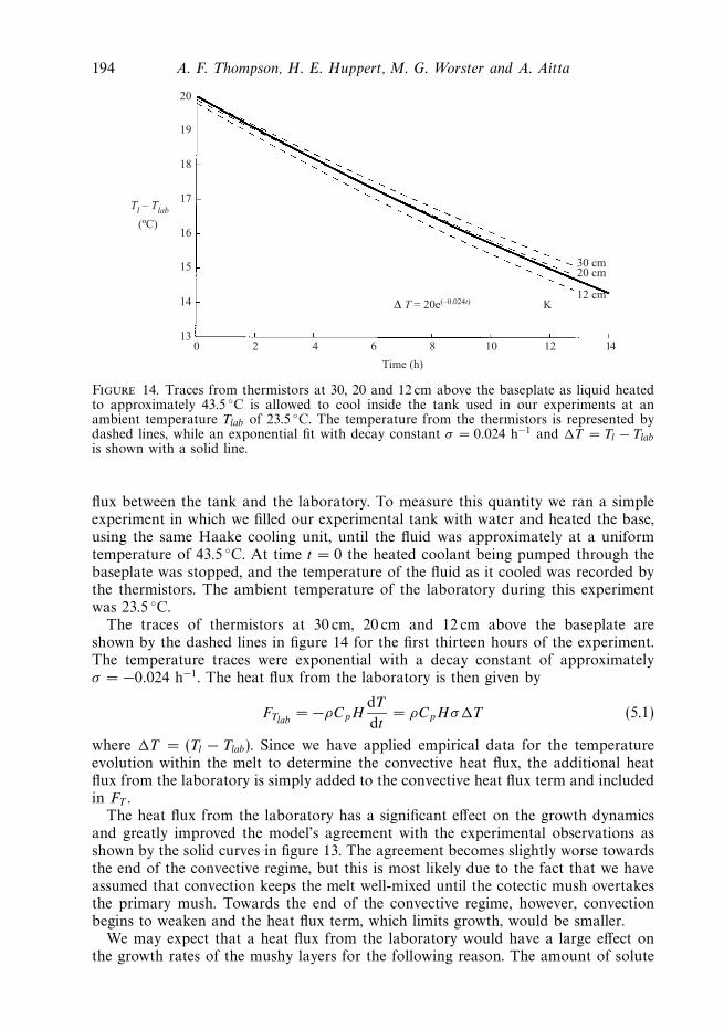
Figure 14. Traces from thermistors at 30, 20 and 12 cm above the baseplate as liquid heatedto approximately 43.5 ◦C is allowed to cool inside the tank used in our experiments at anambient temperature Tlab of 23.5 ◦C. The temperature from the thermistors is represented bydashed lines, while an exponential fit with decay constant σ = 0.024 h−1 and �T = Tl − Tlabis shown with a solid line.
flux between the tank and the laboratory. To measure this quantity we ran a simpleexperiment in which we filled our experimental tank with water and heated the base,using the same Haake cooling unit, until the fluid was approximately at a uniformtemperature of 43.5 ◦C. At time t = 0 the heated coolant being pumped through thebaseplate was stopped, and the temperature of the fluid as it cooled was recorded bythe thermistors. The ambient temperature of the laboratory during this experimentwas 23.5 ◦C.
The traces of thermistors at 30 cm, 20 cm and 12 cm above the baseplate areshown by the dashed lines in figure 14 for the first thirteen hours of the experiment.The temperature traces were exponential with a decay constant of approximatelyσ = −0.024 h−1. The heat flux from the laboratory is then given by
FTlab= −ρCpH
dT
dt= ρCpHσ�T (5.1)
where �T = (Tl − Tlab). Since we have applied empirical data for the temperatureevolution within the melt to determine the convective heat flux, the additional heatflux from the laboratory is simply added to the convective heat flux term and includedin FT .
The heat flux from the laboratory has a significant effect on the growth dynamicsand greatly improved the model’s agreement with the experimental observations asshown by the solid curves in figure 13. The agreement becomes slightly worse towardsthe end of the convective regime, but this is most likely due to the fact that we haveassumed that convection keeps the melt well-mixed until the cotectic mush overtakesthe primary mush. Towards the end of the convective regime, however, convectionbegins to weaken and the heat flux term, which limits growth, would be smaller.
We may expect that a heat flux from the laboratory would have a large effect onthe growth rates of the mushy layers for the following reason. The amount of solute
Solidification and compositional convection of a ternary alloy 195
Time (h)
φ
φBc
φBp
φAc
0 5 10 15 20 25 30
0.1
0.2
0.3
0.4
0.5
0.6
0.7
0.8
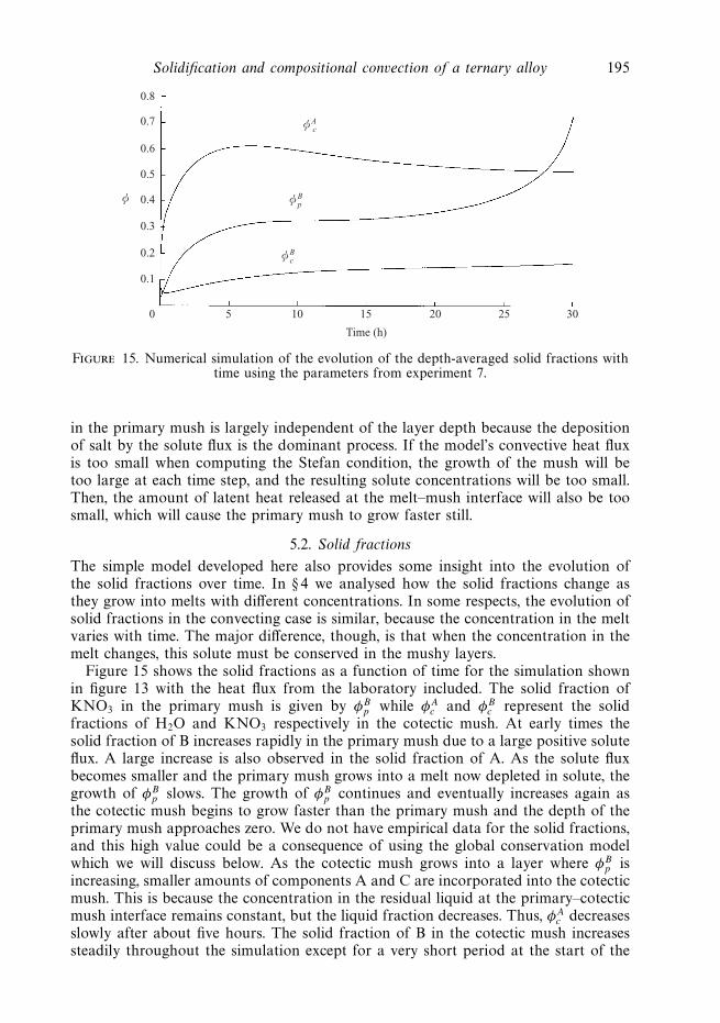
Figure 15. Numerical simulation of the evolution of the depth-averaged solid fractions withtime using the parameters from experiment 7.
in the primary mush is largely independent of the layer depth because the depositionof salt by the solute flux is the dominant process. If the model’s convective heat fluxis too small when computing the Stefan condition, the growth of the mush will betoo large at each time step, and the resulting solute concentrations will be too small.Then, the amount of latent heat released at the melt–mush interface will also be toosmall, which will cause the primary mush to grow faster still.
5.2. Solid fractions
The simple model developed here also provides some insight into the evolution ofthe solid fractions over time. In § 4 we analysed how the solid fractions change asthey grow into melts with different concentrations. In some respects, the evolution ofsolid fractions in the convecting case is similar, because the concentration in the meltvaries with time. The major difference, though, is that when the concentration in themelt changes, this solute must be conserved in the mushy layers.
Figure 15 shows the solid fractions as a function of time for the simulation shownin figure 13 with the heat flux from the laboratory included. The solid fraction ofKNO3 in the primary mush is given by φB
p while φAc and φB
c represent the solidfractions of H2O and KNO3 respectively in the cotectic mush. At early times thesolid fraction of B increases rapidly in the primary mush due to a large positive soluteflux. A large increase is also observed in the solid fraction of A. As the solute fluxbecomes smaller and the primary mush grows into a melt now depleted in solute, thegrowth of φB
p slows. The growth of φBp continues and eventually increases again as
the cotectic mush begins to grow faster than the primary mush and the depth of theprimary mush approaches zero. We do not have empirical data for the solid fractions,and this high value could be a consequence of using the global conservation modelwhich we will discuss below. As the cotectic mush grows into a layer where φB
p isincreasing, smaller amounts of components A and C are incorporated into the cotecticmush. This is because the concentration in the residual liquid at the primary–cotecticmush interface remains constant, but the liquid fraction decreases. Thus, φA
c decreasesslowly after about five hours. The solid fraction of B in the cotectic mush increasessteadily throughout the simulation except for a very short period at the start of the
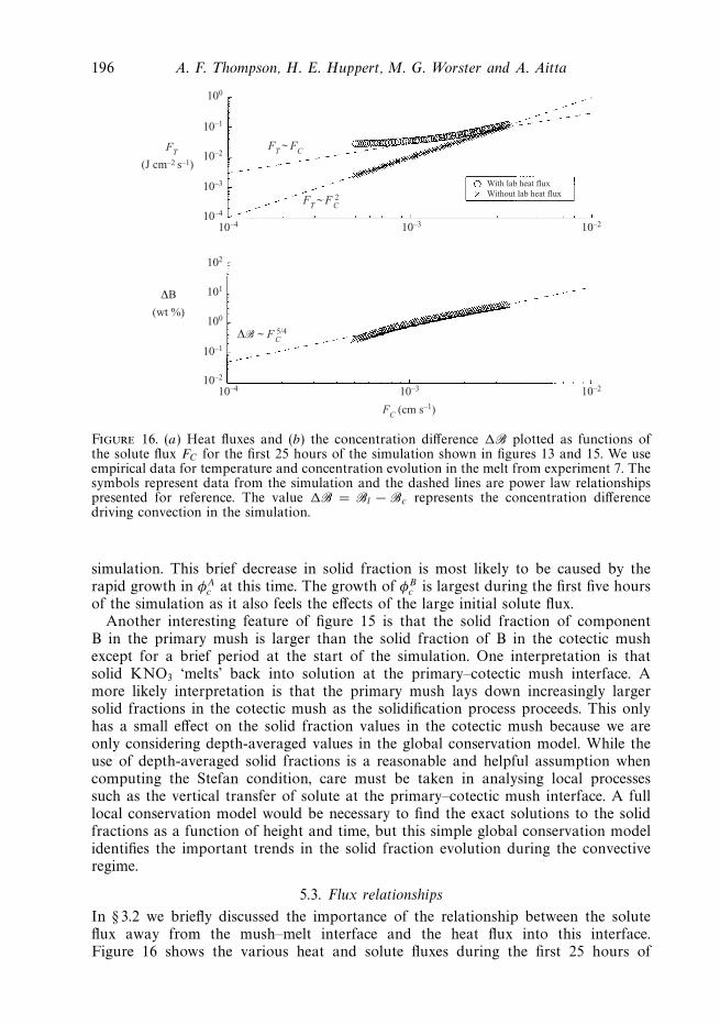
196 A. F. Thompson, H. E. Huppert, M. G. Worster and A. Aitta
10–4 10–3 10–210–4
10–3
10–2
10–1
100
10–4 10–3 10–210–2
10–1
100
101
102
FC (cm s–1)
FT
(J cm–2 s–1)
DB
(wt %)
With lab heat fluxWithout lab heat flux
D� ~ FC5/4
FT ~ FC
FT ~ FC2
Figure 16. (a) Heat fluxes and (b) the concentration difference �B plotted as functions ofthe solute flux FC for the first 25 hours of the simulation shown in figures 13 and 15. We useempirical data for temperature and concentration evolution in the melt from experiment 7. Thesymbols represent data from the simulation and the dashed lines are power law relationshipspresented for reference. The value �B = Bl − Bc represents the concentration differencedriving convection in the simulation.
simulation. This brief decrease in solid fraction is most likely to be caused by therapid growth in φA
c at this time. The growth of φBc is largest during the first five hours
of the simulation as it also feels the effects of the large initial solute flux.Another interesting feature of figure 15 is that the solid fraction of component
B in the primary mush is larger than the solid fraction of B in the cotectic mushexcept for a brief period at the start of the simulation. One interpretation is thatsolid KNO3 ‘melts’ back into solution at the primary–cotectic mush interface. Amore likely interpretation is that the primary mush lays down increasingly largersolid fractions in the cotectic mush as the solidification process proceeds. This onlyhas a small effect on the solid fraction values in the cotectic mush because we areonly considering depth-averaged values in the global conservation model. While theuse of depth-averaged solid fractions is a reasonable and helpful assumption whencomputing the Stefan condition, care must be taken in analysing local processessuch as the vertical transfer of solute at the primary–cotectic mush interface. A fulllocal conservation model would be necessary to find the exact solutions to the solidfractions as a function of height and time, but this simple global conservation modelidentifies the important trends in the solid fraction evolution during the convectiveregime.
5.3. Flux relationships
In § 3.2 we briefly discussed the importance of the relationship between the soluteflux away from the mush–melt interface and the heat flux into this interface.Figure 16 shows the various heat and solute fluxes during the first 25 hours of
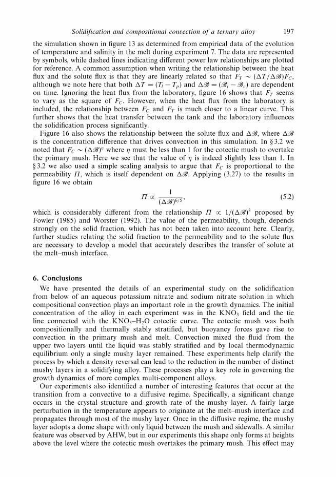
Solidification and compositional convection of a ternary alloy 197
the simulation shown in figure 13 as determined from empirical data of the evolutionof temperature and salinity in the melt during experiment 7. The data are representedby symbols, while dashed lines indicating different power law relationships are plottedfor reference. A common assumption when writing the relationship between the heatflux and the solute flux is that they are linearly related so that FT ∼ (�T/�B)FC ,although we note here that both �T = (Tl − Tp) and �B = (Bl − Bc) are dependenton time. Ignoring the heat flux from the laboratory, figure 16 shows that FT seemsto vary as the square of FC . However, when the heat flux from the laboratory isincluded, the relationship between FC and FT is much closer to a linear curve. Thisfurther shows that the heat transfer between the tank and the laboratory influencesthe solidification process significantly.
Figure 16 also shows the relationship between the solute flux and �B, where �Bis the concentration difference that drives convection in this simulation. In § 3.2 wenoted that FC ∼ (�B)η where η must be less than 1 for the cotectic mush to overtakethe primary mush. Here we see that the value of η is indeed slightly less than 1. In§ 3.2 we also used a simple scaling analysis to argue that FC is proportional to thepermeability Π , which is itself dependent on �B. Applying (3.27) to the results infigure 16 we obtain
Π ∝ 1
(�B)6/5, (5.2)
which is considerably different from the relationship Π ∝ 1/(�B)3 proposed byFowler (1985) and Worster (1992). The value of the permeability, though, dependsstrongly on the solid fraction, which has not been taken into account here. Clearly,further studies relating the solid fraction to the permeability and to the solute fluxare necessary to develop a model that accurately describes the transfer of solute atthe melt–mush interface.
6. ConclusionsWe have presented the details of an experimental study on the solidification
from below of an aqueous potassium nitrate and sodium nitrate solution in whichcompositional convection plays an important role in the growth dynamics. The initialconcentration of the alloy in each experiment was in the KNO3 field and the tieline connected with the KNO3–H2O cotectic curve. The cotectic mush was bothcompositionally and thermally stably stratified, but buoyancy forces gave rise toconvection in the primary mush and melt. Convection mixed the fluid from theupper two layers until the liquid was stably stratified and by local thermodynamicequilibrium only a single mushy layer remained. These experiments help clarify theprocess by which a density reversal can lead to the reduction in the number of distinctmushy layers in a solidifying alloy. These processes play a key role in governing thegrowth dynamics of more complex multi-component alloys.
Our experiments also identified a number of interesting features that occur at thetransition from a convective to a diffusive regime. Specifically, a significant changeoccurs in the crystal structure and growth rate of the mushy layer. A fairly largeperturbation in the temperature appears to originate at the melt–mush interface andpropagates through most of the mushy layer. Once in the diffusive regime, the mushylayer adopts a dome shape with only liquid between the mush and sidewalls. A similarfeature was observed by AHW, but in our experiments this shape only forms at heightsabove the level where the cotectic mush overtakes the primary mush. This effect may
198 A. F. Thompson, H. E. Huppert, M. G. Worster and A. Aitta
be due to sidewall heating from the laboratory. In general, the concentration andtemperature evolution of the alloy shows good agreement with the predictions ofthe ternary phase diagram under the assumption of a piecewise linear liquid line ofdescent, and we confirm the corrections made to the KNO3–H2O cotectic curve madeby AHW.
The global conservation model provides a relatively simple and accurate modelfor determining the growth rates of mushy layers although, in the convective modeldescribed here, the heat and solute fluxes must be forced by empirical data. Wehave presented the variation in solid fraction with initial melt concentration in anon-convecting system and compare how this changes in a convecting system wheredecreases in solute content in the melt are reflected by an increase in solid fractionsin order to conserve solute globally. Our model identifies the pronounced effectof heating from the laboratory on the growth rates of mushy layers in a convectingsystem. This may be an important factor in accurately describing natural or industrialsolidification processes where there is an external source of heating or cooling.
We thank Mark Hallworth for his assistance in the laboratory and Geoff Moggridgefor the use of the atomic absorption spectrometer. A.F.T. was supported by a fellowshipfrom the Keasbey Memorial Foundation. A.A. held a Daphne Jackson Fellowshipsupported by Lucy Cavendish College, University of Cambridge, and the ThriplowCharitable Trust.
REFERENCES
Aitta, A., Huppert, H. E. & Worster, M. G. 2001a Solidification in ternary systems. In InteractiveDynamics of Convection and Solidification (ed. P. Ehrhard, D. S. Riley & P. H. Steen), pp. 113–122. Kluwer.
Aitta, A., Huppert, H. E. & Worster, M. G. 2001b Diffusion-controlled solidification of a ternarymelt from a cooled boundary. J. Fluid Mech. 432, 201–217 (herein referred to as AHW).
Anderson, D. M. 2003 A model for diffusion-controlled solidification of ternary alloys in mushylayers. J. Fluid Mech. 483, 165–197.
Batchelor, G. K. 1974 Transport properties of two-phase materials with random structure. Annu.Rev. Fluid Mech. 6, 227–255.
Bloomfield, L. J. & Huppert, H. E. 2003 Solidification and convection of a ternary solution cooledfrom the side. J. Fluid Mech. 489, 269–299.
Chen, C. F. & Chen, F. 1991 Experimental study of directional solidification of aqueous ammoniumchloride solution. J. Fluid Mech. 227, 567–586.
Copley, S. M., Giamei, A. F., Johnson, S. M. & Hornbecker, M. F. 1970 The origin of freckles inunidirectionally solidified castings. Metall. Trans. 1, 2193–2204.
Fowler, A. C. 1985 The formation of freckles in binary alloys. IMA J. Appl. Maths 35, 159–174.
Huppert, H. E. 1990 The fluid mechanics of solidification. J. Fluid Mech. 212, 209–240.
Huppert, H. E. & Sparks, R. S. J. 1980 Restrictions on the composition of mid-ocean ridge basalts:a fluid dynamical investigation. Nature 286, 46–48.
Huppert, H. E. & Sparks, R. S. J. 1984 Double-diffusive convection due to crystallization inmagmas. Annu. Rev. Earth Planet. Sci. Lett. 12, 11–37.
Huppert, H. E. & Worster, M. G. 1985 Dynamic solidification of a binary melt. Nature 314,703–707.
Huppert, H. E. & Worster, M. G. 1991 Vigorous motions in magma chambers and lava lakes.IMA Proceedings–Preprint Series 862.
Kerr, R. C., Woods, A. W., Worster, M. G. & Huppert, H. E. 1990a Solidification of an alloycooled from above. Part 2. Non-equilibrium interfacial kinetics. J. Fluid Mech. 217, 331–348.
Kerr, R. C., Woods, A. W., Worster, M. G. & Huppert, H. E. 1990b Solidification of an alloycooled from above. Part 3. Compositional stratification within the solid. J. Fluid Mech. 218,337–354.
Solidification and compositional convection of a ternary alloy 199
Lide, D. R. 1997 CRC Handbook of Chemistry and Physics, 78th Edn. CRC Press.
Mullins, W. W. & Sekerka, R. F. 1964 Stability of a planar interface during solidification of adilute binary alloy. J. Appl. Phys. 35, 444–451.
Phillips, O. M. 1991 Flow and Reactions in Permeable Rocks. Cambridge University Press.
Sarazin, J. R. & Hellawell, A. 1992 Studies of channel-plume convection during solidification.In Interactive Dynamics of Convection and Solidification (ed. S. H. Davis, H. E. Huppert,U. Muller & M. G. Worster), pp. 143–145. Kluwer.
Tait, S. & Jaupart, C. 1992 Compositional convection in a reactive crystalline mush and meltdifferentiation. J. Geophys. Res. 97, B5, 6735–6756.
Thompson, A. F., Huppert, H. E. & Worster, M. G. 2003 Appendix: A global conservation modelfor diffusion-controlled solidification of a ternary alloy. J. Fluid Mech. 483, 191–197.
Turner, J. S., Huppert, H. E., & Sparks, R. S. J. 1986 Komatiites II: Experimental and theoreticalinvestigations of post-emplacement cooling and crystallization. J. Petrol. 27, 397–437.
West, D. R. F. 1982 Ternary Equilibrium Diagrams, 2nd Edn. Chapman and Hall.
Wettlaufer, J. S., Worster, M. G. & Huppert, H. E. 1997 Natural convection during solidificationof an alloy from above with application to the evolution of sea ice. J. Fluid Mech. 344, 291–316.
Wettlaufer, J. S., Worster, M. G. & Huppert, H. E. 2000 The solidification of leads: Theory,experiment and field observations. J. Geophys. Res. 105, 1123–1134.
Woods, A. W. & Huppert, H. E. 1989 The growth of compositionally stratified solid above ahorizontal boundary. J. Fluid Mech. 199, 29–53.
Worster, M. G. 1990 Structure of a convecting mushy layer. Appl. Mech. Rev. 43, 5, S59–S62.
Worster, M. G. 1991 Natural convection in a mushy layer. J. Fluid Mech. 224, 335–359.
Worster, M. G. 1992 The dynamics of mushy layers. In Interactive Dynamics of Convection andSolidification (ed. S. H. Davis, H. E. Huppert, U. Muller & M. G. Worster), pp. 113–138.Kluwer.
Worster, M. G. 2000 Solidification of Fluids. In Perspectives in Fluid Dynamics (ed. G. K. Batchelor,H. K. Moffatt & M. G. Worster), pp. 393–446. Cambridge University Press.