solid oxide fuel cell system control - skemman · solid oxide fuel cell system control ... matlab...
TRANSCRIPT
Solid Oxide Fuel Cell System Control
Modeling and Control Study of a Catalytic Partial Oxidation (CPOX) Reactor
Tomasz S. Miklis
SOLID OXIDE FUEL CELL SYSTEM CONTROL
Modeling and Control Study of a Catalytic Partial Oxidation (CPOX) Reactor
Tomasz Szczęsny Miklis
A 30 credit units Master’s thesis
Supervisors:
Dr. Tyrone Vincent (Project advisor)
Dr. David Dvorak (Academic advisor)
Dr. Thorsteinn Ingi Sigfusson (Academic advisor)
A Master’s thesis done at
RES │ the School for Renewable Energy Science
in affiliation with
University of Iceland &
the University of Akureyri
Akureyri, February 2009
Solid Oxide Fuel Cell System Control
Modeling and Control Study of a Catalytic Partial Oxidation (CPOX) Reactor
A 30 credit units Master’s thesis
© Tomasz Szczęsny Miklis, 2009
RES │ the School for Renewable Energy Science
Solborg at Nordurslod
IS600 Akureyri, Iceland
telephone: + 354 464 0100
www.res.is
Printed in 14/05/2009
at Stell Printing in Akureyri, Iceland
iii
ABSTRACT
An advanced thermodynamic model of a catalytic partial oxidation (CPOX) reactor was
developed. The dynamics of the reactor were simulated using differential algebraic
equations (DAEs). The aim of the project was to create a reliable and fast model that will
be used, for control purposes, to maximize the hydrogen yield from the CPOX reaction.
The composition of the output flow and species concentration is controlled by the input
mass flows of fuel (Dodecane) and air. The state variables of the reactor considered in this
model are temperature and total internal energy of the reactor. There are many options
with which to customize the reactor model, from the geometry and materials used to build
the reactor shell to different compositions of the gases fed to the reactor (fuel and air). The
Cantera toolbox was used to simulate chemistry and the whole project was completed the
in MATLAB programming environment.
iv
PREFACE
The focus of this Master Thesis project for the Fuel Cell Systems & Hydrogen
specialization at RES | The School for Renewable Energy Science is Solid Oxide Fuel Cell
System Control. At my home university (AGH University of Science and Technology in
Kraków) I am doing continuous M.Sc. studies in Automatics and Robotics specializing in
Computer Science in Control and Management. My goal with this thesis is to study the
control aspect of fuel cell systems and continue this research with my engineering M.Sc.
thesis at my home university.
Ryan O‟Hayre and Neal Sullivan, the Professors from the Colorado School of Mines, were
lecturers at the RES | The School for Renewable Energy Science (FC602 Fuel Cell Types
& Technologies course) in July 2008. During that time the idea of completing my M.Sc.
project in Colorado was born. Thanks to the excellent cooperation between CSM and RES,
I completed my thesis in the United States.
This project was developed during my work as a research associate at the Colorado School
of Mines in Golden from 21st of October 2008 till 2
nd of February 2009. My research was
supervised Dr Tyrone Vincent. I was part of the Control Group of the Department of
Energy (DOE) research grant.
I would like to give thanks for all the support I received during my work at CSM. There
were many kind and helpful people I encountered during my work on this project. I would
especially like to thank:
Mr. Tyrone Vincent – for being my advisor and always finding time to answer my
questions and guide me with my research;
Mr. Bob Kee – for all the support with building the thermodynamic formulation of
the CPOX reactor;
Mr. Huayang Zhu – for his help with the chemistry behind the CPOX reactor and
comparing results of this model with others;
Mr. Borhan Sanandaji – for his cooperation and help with the control aspects of
the project;
Mr. Kevin Moore – for his willingness to host me at CSM and initializing my
project;
Mr. Neal Sullivan – for helping to organize the legal aspects of this project;
Mr. David Dvorak – for his help with final revisions of the thesis report;
Mr. Thorsteinn Ingi Sigfusson – for coordinating my specialization;
RES staff – for organizing the stay in United Stated and help with many day-to-day
problems;
RES teachers – for preparing me to work on the M.Sc. project;
Fellow RES 2008/2009 students – for a great year at the RES School.
Golden, 02.02.2009
v
TABLE OF CONTENTS
1 Project Overview .............................................................................................................. 1
1.1 Introduction ................................................................................................................ 1
1.2 US Department of Energy (DOE) research project ................................................... 2
1.3 Multimedia aspects of the project .............................................................................. 2
1.3.1 Box.net data exchange space ............................................................................ 2
1.3.2 Control Wiki ..................................................................................................... 3
2 Review of Fuel Cell Control publications ........................................................................ 5
3 Solid Oxide Fuel Cell System ........................................................................................... 6
3.1 The promise of Fuel Cells .......................................................................................... 6
3.2 Solid Oxide Fuel Cell – „the heart‟ ............................................................................ 7
3.3 Balance-of-Plant components – „the body‟ ............................................................... 8
3.4 Control Units – „the brains‟ ....................................................................................... 9
4 Control Theory Overview ............................................................................................... 10
4.1 Basics of Control Theory ......................................................................................... 10
4.2 State-space representation ....................................................................................... 11
4.3 System Identification ............................................................................................... 11
4.4 Model-Based Control Methods ................................................................................ 12
4.5 CPOX Reactor Model .............................................................................................. 12
5 Chemical Equilibrium ..................................................................................................... 13
5.1 Theory behind chemical equilibrium ....................................................................... 13
5.2 STANJAN and the Element-Potential Method ........................................................ 14
5.3 CHEMKIN EQUIL .................................................................................................. 15
5.4 CANTERA .............................................................................................................. 15
5.4.1 MATLAB Cantera toolbox ............................................................................ 16
6 Catalytic Partial Oxidation (CPOX) Reactor Model ...................................................... 17
6.1 Fuel reforming overview ......................................................................................... 17
6.2 Calculating the C/O ratio ......................................................................................... 18
6.3 Model description .................................................................................................... 19
7 Differential Algebraic Equations .................................................................................... 23
7.1 Theory behind DAEs ............................................................................................... 23
7.2 CPOX reactor mathematical model ......................................................................... 24
8 Model testing .................................................................................................................. 27
8.1 Implicit problem formulation (MATLAB fzero solution) ....................................... 27
vi
8.2 DAE problem formulation (MATLAB ode15s solution) ........................................ 28
8.3 Model Results .......................................................................................................... 29
8.3.1 Startup Transients ........................................................................................... 29
8.3.2 Species concentrations ................................................................................... 30
9 Future Project Development ........................................................................................... 33
10 Conclusions ..................................................................................................................... 35
References ........................................................................................................................... 37
APPENDIX A: MATLAB Implementations ......................................................................... 1
APPENDIX C: Graphs .......................................................................................................... 3
vii
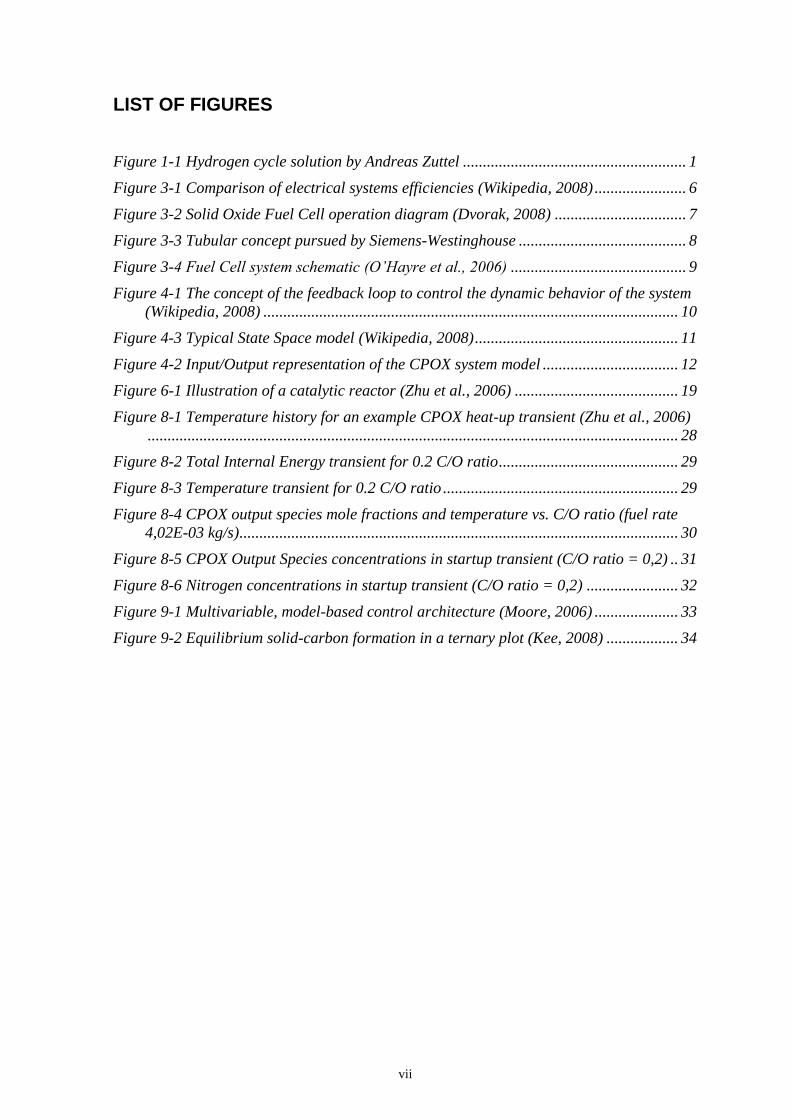
LIST OF FIGURES
Figure 1-1 Hydrogen cycle solution by Andreas Zuttel ........................................................ 1
Figure 3-1 Comparison of electrical systems efficiencies (Wikipedia, 2008) ....................... 6
Figure 3-2 Solid Oxide Fuel Cell operation diagram (Dvorak, 2008) ................................. 7
Figure 3-3 Tubular concept pursued by Siemens-Westinghouse .......................................... 8
Figure 3-4 Fuel Cell system schematic (O’Hayre et al., 2006) ............................................ 9
Figure 4-1 The concept of the feedback loop to control the dynamic behavior of the system
(Wikipedia, 2008) ........................................................................................................ 10
Figure 4-3 Typical State Space model (Wikipedia, 2008) ................................................... 11
Figure 4-2 Input/Output representation of the CPOX system model .................................. 12
Figure 6-1 Illustration of a catalytic reactor (Zhu et al., 2006) ......................................... 19
Figure 8-1 Temperature history for an example CPOX heat-up transient (Zhu et al., 2006)
..................................................................................................................................... 28
Figure 8-2 Total Internal Energy transient for 0.2 C/O ratio ............................................. 29
Figure 8-3 Temperature transient for 0.2 C/O ratio ........................................................... 29
Figure 8-4 CPOX output species mole fractions and temperature vs. C/O ratio (fuel rate
4,02E-03 kg/s) .............................................................................................................. 30
Figure 8-5 CPOX Output Species concentrations in startup transient (C/O ratio = 0,2) .. 31
Figure 8-6 Nitrogen concentrations in startup transient (C/O ratio = 0,2) ....................... 32
Figure 9-1 Multivariable, model-based control architecture (Moore, 2006) ..................... 33
Figure 9-2 Equilibrium solid-carbon formation in a ternary plot (Kee, 2008) .................. 34
viii
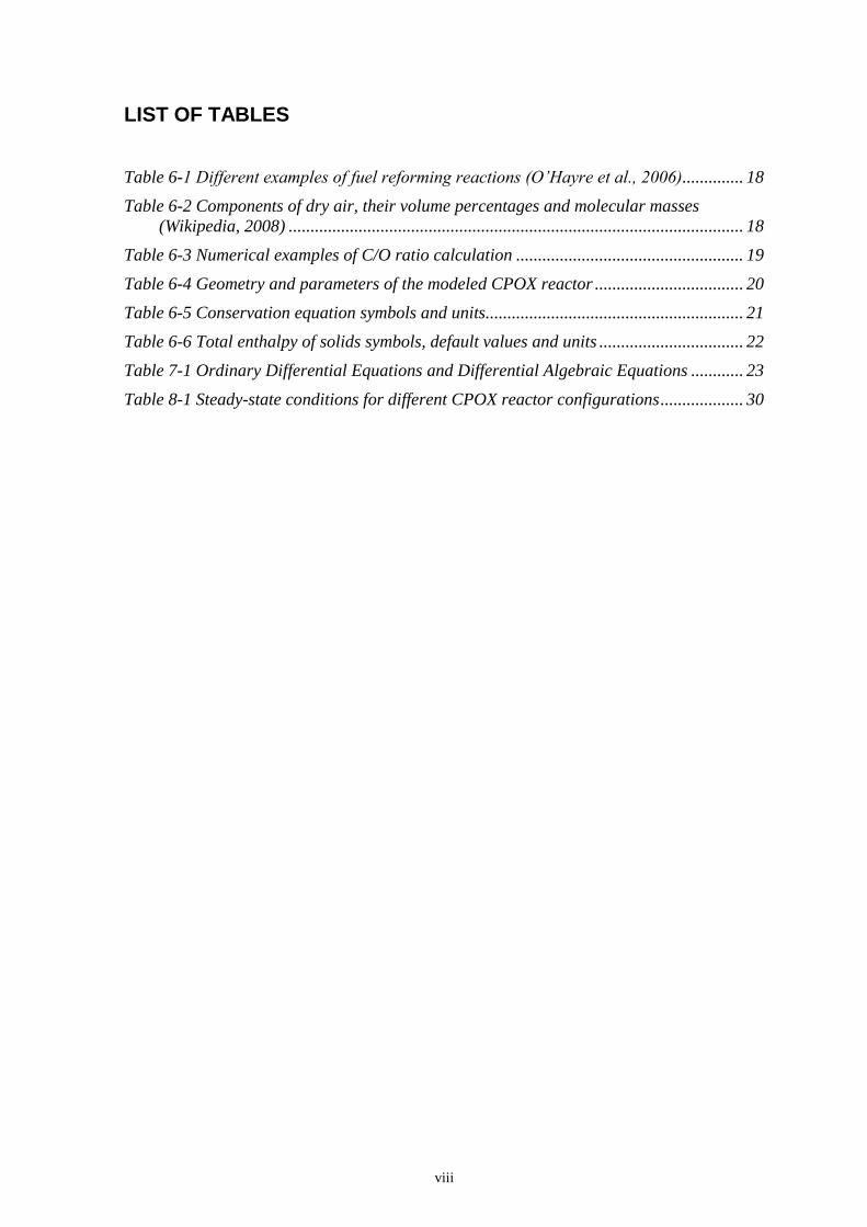
LIST OF TABLES
Table 6-1 Different examples of fuel reforming reactions (O’Hayre et al., 2006).............. 18
Table 6-2 Components of dry air, their volume percentages and molecular masses
(Wikipedia, 2008) ........................................................................................................ 18
Table 6-3 Numerical examples of C/O ratio calculation .................................................... 19
Table 6-4 Geometry and parameters of the modeled CPOX reactor .................................. 20
Table 6-5 Conservation equation symbols and units........................................................... 21
Table 6-6 Total enthalpy of solids symbols, default values and units ................................. 22
Table 7-1 Ordinary Differential Equations and Differential Algebraic Equations ............ 23
Table 8-1 Steady-state conditions for different CPOX reactor configurations ................... 30
1
1 PROJECT OVERVIEW
This study focused on the modeling of the Catalytic Partial Oxidation (CPOX) reactor in
the Solid Oxide Fuel Cell system. The overall aim of the US Department of Energy (DOE)
research grant, of which this research is an important component, is to develop a flexible
and fast model of a whole system containing fuel cell stack, CPOX reactor and balance-of-
plant components. This research models the fuel processor element of the system. The
output species composition is estimated based on the different mass flows of inlet streams
(Dodecane and air). This information is necessary to develop control schemes that will
maximize the yield of the hydrogen from CPOX reaction.
An advanced thermodynamic model was designed and formulated using differential
algebraic equations. MATLAB software with the Cantera toolbox, to simulate the
complicated chemistry, was used for numerical simulations.
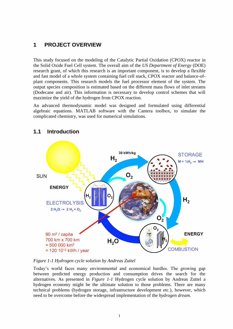
1.1 Introduction
Figure 1-1 Hydrogen cycle solution by Andreas Zuttel
Today‟s world faces many environmental and economical hurdles. The growing gap
between predicted energy production and consumption drives the search for the
alternatives. As presented in Figure 1-1 Hydrogen cycle solution by Andreas Zuttel a
hydrogen economy might be the ultimate solution to those problems. There are many
technical problems (hydrogen storage, infrastructure development etc.), however, which
need to be overcome before the widespread implementation of the hydrogen dream.
2
The solid oxide fuel cell (SOFC) systems with CPOX reactors that can process
hydrocarbon fuels to create hydrogen will be a very important intermediate step on the way
to a hydrogen economy, from a short term perspective.
1.2 US Department of Energy (DOE) research project
This research was a part of the US Department of Energy (DOE) research grant:
“Renewable and Logistic Fuels for Fuel Cells at the Colorado School of Mines”
Starting Date: 01.05.2008
Duration: 2 years
Budget: $1,476,000
“The objective of this program is to advance the current state of technology of solid-oxide
fuel cells (SOFCs) to improve performance when operating on renewable and logistics
hydrocarbons fuel streams.”
This project is aimed at answering some of the problems formulated in the Task 3.0:
Balance-of-Plant Development, System Optimization and Control.
The goal of the Fuel Cell System Control task is the design of a control system to regulate
the operation of a complete system based on an SOFC stack. The control system design is
based on a dynamic model that can predict system behavior given perturbations in actuator
settings, such as air and fuel flows and power loads. Ideally, these models are based on
physical first principles. However, physically based models are often very complex and
take considerable computational resources to compute. For some activities, computational
complexity can become a limiting factor in the usefulness of the model, and it becomes
necessary to capture the dominant behavior in a lower order model that can be run quickly.
This is especially true when the models are used with a real-time, or on-line automated
activity, such as process monitoring and control, but this can also be useful when building
interconnected or hierarchical models that can be run in a reasonable amount of time. As
part of this project, we have developed a model reduction that can capture both the linear
and nonlinear behavior of physics based models. These reduced models are then utilized
within a Model Predictive Control (MPC) implementation for integrated control of the fuel
cell stack and associated balance of plant components.
1.3 Multimedia aspects of the project
There was a significant effort put into making the results of this project accessible and to
develop a platform for international cooperation for the future development of this
research.
1.3.1 Box.net data exchange space
All the MATLAB source codes, most of the references used in this report and installation
files of the Cantera toolbox are available at the box.net server. The collaborator of the
project can access all those files by using this address:

3
http://www.box.net/shared/86oa2k4d53
1.3.2 Control Wiki
The Control Wiki website was created to allow easy tracking of the current progress of the
research. An outline of the research activities, some results, and important references are
regularly published there. The collaborator of the project can access that information by
using this address:
http://control.mines.edu/mediawiki/index.php/Control_of_Solid_Oxide_Fuel_Cells

5
2 REVIEW OF FUEL CELL CONTROL PUBLICATIONS
The control aspect of fuel cell systems is a relatively unexplored area of research. There is
a limited amount of publications, most of which originate from the University of Michigan.
A research group that focuses on the control of the fuel cell systems is led by Anna G.
Stefanopoulou. Their research is connected to low-temperature polymer exchange
membrane (PEM) fuel cells (Pukrushpan, Stefanopoulou, & Peng, 2004).
The current studies proved that the response of a fuel cell system depends on the air and
hydrogen feed, flow and pressure regulation, and heat and water management. Dynamic
models of PEM FC systems suitable for the control study were developed. The fuel cell
stack temperature is treated as a parameter rather than state variable, which is a serious
limitation (Pukrushpan, Peng, & Stefanopoulou, Control-Oriented Modeling and Analysis
for Automotive Fuel Cell Systems, 2004).
6
3 SOLID OXIDE FUEL CELL SYSTEM
This chapter will introduce some basic knowledge about fuel cells. First, a brief history of
this energy generating device will be presented, followed by a technical description of the
working principles of Solid Oxide Fuel Cell System.
3.1 The promise of Fuel Cells
Although fuel cells (FC) seem like a twenty-first-century marvel, they are a nineteenth-
century invention that predates the innovation of the internal combustion engine. The
invention of fuel cells as an electrical energy conversion system is attributed to Sir William
Grove (Carrette, Friedrich, & Stimming, 2001). For more than 150 years fuel cells have
presented the promise of zero emission energy generation.
The hype about fuel cells gained momentum after the National Aeronautics and Space
Administration (NASA) used them in the 60‟s with the Apollo program. The alkaline fuel
cells did a good job in the sterile deep space environment. Unfortunately, „back on Earth‟
they were easily poisoned with CO2, which limited their commercial application. After the
Oil Crisis hit the world in the 1973, fuel cells were again in the spotlight. The biggest
problem for wide commercial application was, and still is, fuel storage. Because of its low
volumetric density, energy-reach hydrogen storage is quite problematic. Rare and
expensive Platinum, the catalyst that speeds up the reactions inside FC, is another
difficulty. Even though recently scientists managed to reduce the amount of this precious
metal used in FC systems by a factor of 10, it is a still limiting factor in wider applications.
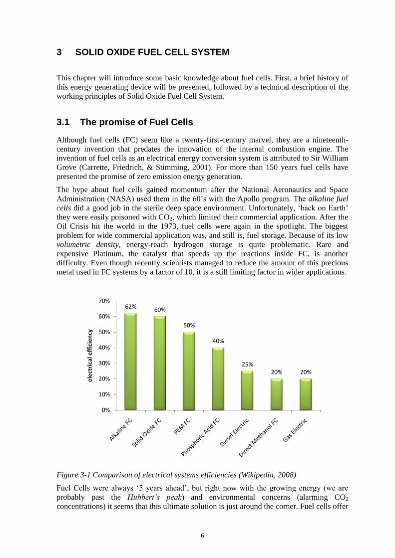
Figure 3-1 Comparison of electrical systems efficiencies (Wikipedia, 2008)
Fuel Cells were always „5 years ahead‟, but right now with the growing energy (we are
probably past the Hubbert’s peak) and environmental concerns (alarming CO2
concentrations) it seems that this ultimate solution is just around the corner. Fuel cells offer
62% 60%
50%
40%
25%20% 20%
0%
10%
20%
30%
40%
50%
60%
70%
ele
ctri
cal e
ffic
ien
cy

7
tremendous promise for solving a variety of energy needs, ranging from portable to
automobile to stationary power. With their high efficiencies (see Figure 3-1 Comparison of
electrical systems efficiencies) and zero emissions, they will reduce our global dependence
on oil and foster future energy security, prosperity, and a cleaner environment. Extensive
government-funded research and the growing activity of the private sector build a much
needed momentum for extensive fuel cell utilization.
3.2 Solid Oxide Fuel Cell – ‘the heart’
Solid oxide fuel cells (SOFCs) use ceramic as the electrolyte. They operate at very high
temperatures– up to 1000°C– and can operate with air and natural gas (or other fuels) as
direct inputs. In contrast to proton exchange membrane (PEM) fuel cells (in which
positively charged hydrogen ions travel through the polymer membrane), SOFCs use
negatively charged oxygen ions that travel through a porous anode, where they combine
with the hydrogen to form water (see Figure 3-2 Solid Oxide Fuel Cell operation diagram).
The solid ceramic electrolyte is a hermetic barrier between the chemical reactants, so no
hydrogen or water can reach the air side of the fuel cell, which simplifies operation
(Romm, 2005). One of the biggest advantages of these systems is that they can use
relatively impure hydrocarbon fuels. The downside is the slow thermal response that
causes long start-up times (Dvorak, Fuel Cell Operation, 2008).
Figure 3-2 Solid Oxide Fuel Cell operation diagram (Dvorak, 2008)
There are two chemical equations that govern SOFC work. The anode reaction
,
and the cathode reaction
8
.
Those formulas sum up to the overall reaction
.
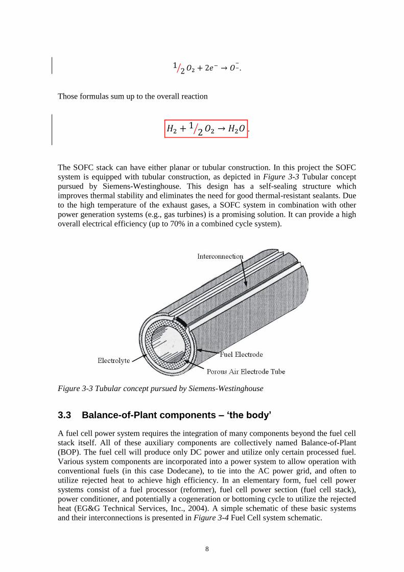
The SOFC stack can have either planar or tubular construction. In this project the SOFC
system is equipped with tubular construction, as depicted in Figure 3-3 Tubular concept
pursued by Siemens-Westinghouse. This design has a self-sealing structure which
improves thermal stability and eliminates the need for good thermal-resistant sealants. Due
to the high temperature of the exhaust gases, a SOFC system in combination with other
power generation systems (e.g., gas turbines) is a promising solution. It can provide a high
overall electrical efficiency (up to 70% in a combined cycle system).
Figure 3-3 Tubular concept pursued by Siemens-Westinghouse
3.3 Balance-of-Plant components – ‘the body’
A fuel cell power system requires the integration of many components beyond the fuel cell
stack itself. All of these auxiliary components are collectively named Balance-of-Plant
(BOP). The fuel cell will produce only DC power and utilize only certain processed fuel.
Various system components are incorporated into a power system to allow operation with
conventional fuels (in this case Dodecane), to tie into the AC power grid, and often to
utilize rejected heat to achieve high efficiency. In an elementary form, fuel cell power
systems consist of a fuel processor (reformer), fuel cell power section (fuel cell stack),
power conditioner, and potentially a cogeneration or bottoming cycle to utilize the rejected
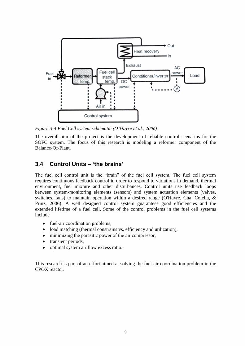
heat (EG&G Technical Services, Inc., 2004). A simple schematic of these basic systems
and their interconnections is presented in Figure 3-4 Fuel Cell system schematic.
9
Figure 3-4 Fuel Cell system schematic (O’Hayre et al., 2006)
The overall aim of the project is the development of reliable control scenarios for the
SOFC system. The focus of this research is modeling a reformer component of the
Balance-Of-Plant.
3.4 Control Units – ‘the brains’
The fuel cell control unit is the “brain” of the fuel cell system. The fuel cell system
requires continuous feedback control in order to respond to variations in demand, thermal
environment, fuel mixture and other disturbances. Control units use feedback loops
between system-monitoring elements (sensors) and system actuation elements (valves,
switches, fans) to maintain operation within a desired range (O'Hayre, Cha, Colella, &
Prinz, 2006). A well designed control system guarantees good efficiencies and the
extended lifetime of a fuel cell. Some of the control problems in the fuel cell systems
include
fuel-air coordination problems,
load matching (thermal constrains vs. efficiency and utilization),
minimizing the parasitic power of the air compressor,
transient periods,
optimal system air flow excess ratio.
This research is part of an effort aimed at solving the fuel-air coordination problem in the
CPOX reactor.

10
4 CONTROL THEORY OVERVIEW
In this chapter, the question “How are models created and used in control systems?” will
be answered. A brief introduction to the main ideas in the modern control theory will be
presented (state space representation, system identification). This introductory knowledge
is necessary to follow the concepts in the subsequent chapters.
4.1 Basics of Control Theory
Control engineering is based on the foundation of feedback theory and linear system
analysis, and it integrates the concepts of network theory and communication theory (Dorf
& Bishop, 2008). A control system is an interconnection of components forming a system
configuration that will provide a desired system response. The basis for the analysis of a
system is the foundation provided by linear system theory, which assumes a cause-effect
relationship for the components of a system. This is why a component or process that will
be controlled can be represented by a block (see Figure 4-1 The concept of the feedback
loop to control the dynamic behavior of the system). The input-output relationship
represents the cause-and-effect relationship of the process, which in turn represents a
processing of the input signal to provide an output signal variable. In this case, the process
is defined as fuel reforming in the CPOX reactor. There are two main types of control
systems:
open-loop control system (utilizes an actuating device to control the process
directly without using feedback),
closed-loop feedback control system (uses a measurement of the output and
feedback of this signal to compare it with the desired output – reference or
command).
Figure 4-1 The concept of the feedback loop to control the dynamic behavior of the system
(Wikipedia, 2008)
Mathematical models of physical systems are key elements in the design and analysis of
control systems. It is necessary to analyze the relationship between the system variables to
obtain a mathematical model. In most cases the systems are dynamic in nature; the
descriptive equations are usually differential equations (see Chapter 7). Those equations
are obtained by utilizing the physical laws of the process. This approach applies equally
well to mechanical, electrical, fluid and the focus of this project – thermodynamic systems.
If these equations can be linearized, then the Laplace transform can be used to simplify the
method of solution. In practice, the complexity of systems and the limited computational
power require the introduction of assumptions concerning the system operation.
11
4.2 State-space representation
State-space representation is a mathematical model of a physical system as a set of input,
output and state variables related by first-order differential equations.
For a dynamic system, the state of a system is described in terms of a set of state variables
. The state variables describe the present configuration of a system
and can be used to determine the future response, given the excitation inputs and the
equations describing the dynamics. In the case of the CPOX reactor, the state variables
are total internal energy ( ) and temperature ( ).
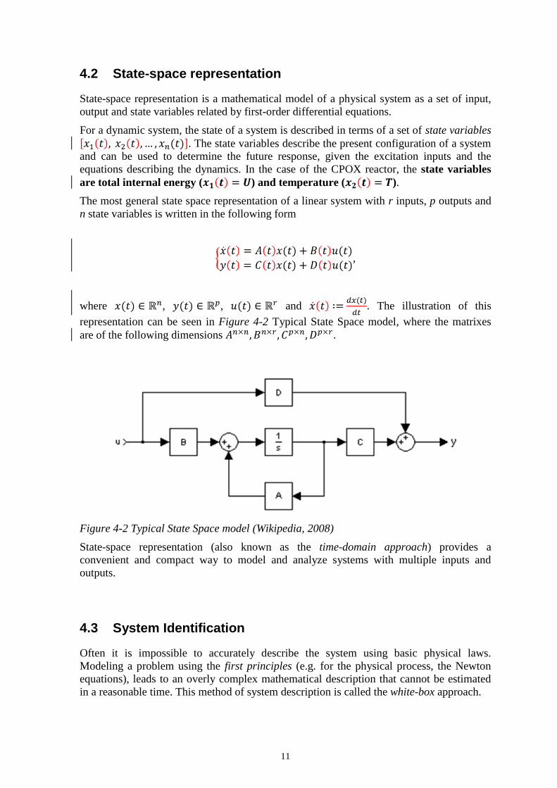
The most general state space representation of a linear system with r inputs, p outputs and
n state variables is written in the following form
,
where , , and . The illustration of this
representation can be seen in Figure 4-2 Typical State Space model, where the matrixes
are of the following dimensions .
Figure 4-2 Typical State Space model (Wikipedia, 2008)
State-space representation (also known as the time-domain approach) provides a
convenient and compact way to model and analyze systems with multiple inputs and
outputs.
4.3 System Identification
Often it is impossible to accurately describe the system using basic physical laws.
Modeling a problem using the first principles (e.g. for the physical process, the Newton
equations), leads to an overly complex mathematical description that cannot be estimated
in a reasonable time. This method of system description is called the white-box approach.
12
A more common approach is to start from measurements of the behavior of the system and
the external influences (inputs to the system). It is important to correctly design the test
signals so that the whole dynamics can be obtained from the test data. In this project, the
PRBS (Pseudo-Random-Binary-Sequence) signals were used for the system identification
of the SOFC stack. After obtaining the test data, a set of candidate models is created by
specifying their common properties. The next step is to find the best model in this set
(Yucai, 2001). For more information about this process see APPENDIX C: .
4.4 Model-Based Control Methods
System models are necessary for a variety of different control methods. One of them is
Linear Time-Invariant Controllers, which is very popular in the electrical, mechanical and
aerospace industries. Another example is Model Predictive Control (MPC), which has a
long history in chemical plants and oil refineries. This multivariable control algorithm uses
an internal dynamic model of the process and a history of past control moves for the
optimization of the cost function. Generally, model-based control systems demonstrate
better control results.
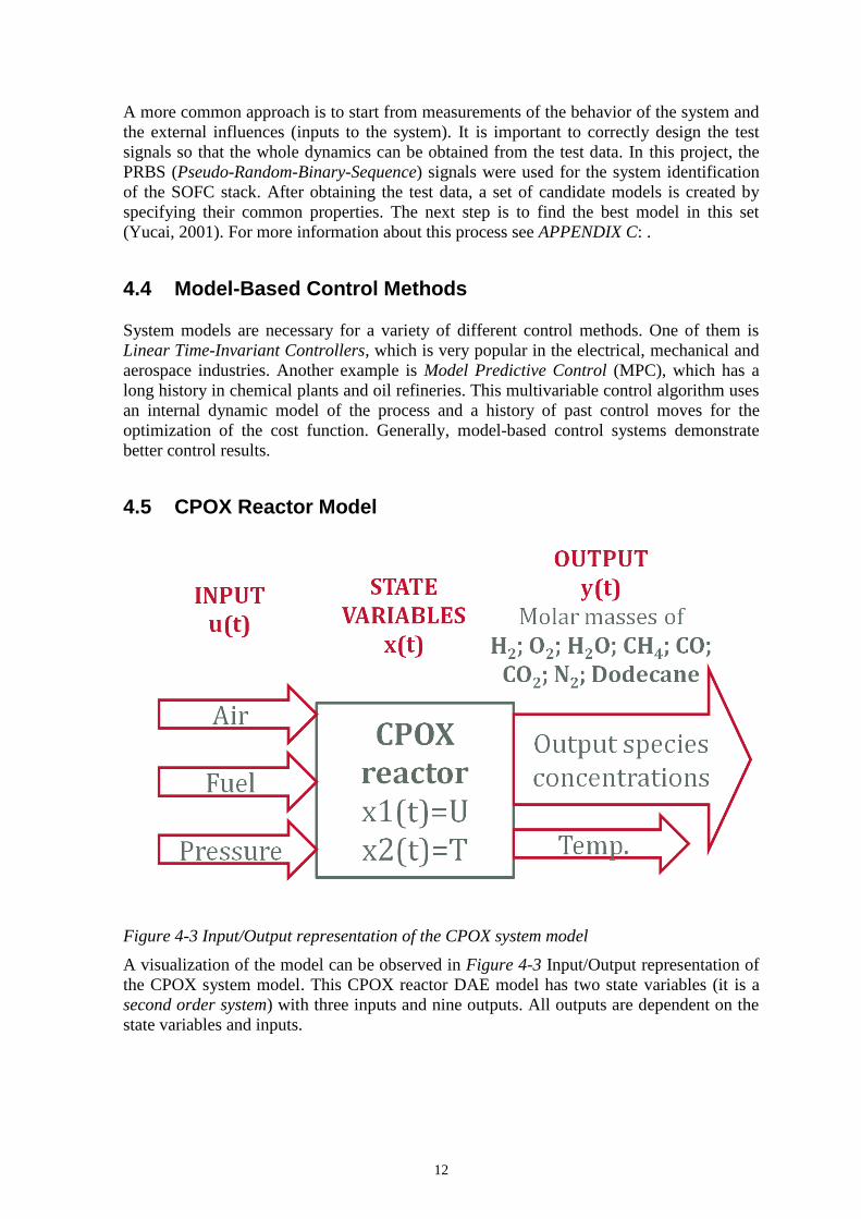
4.5 CPOX Reactor Model
Figure 4-3 Input/Output representation of the CPOX system model
A visualization of the model can be observed in Figure 4-3 Input/Output representation of
the CPOX system model. This CPOX reactor DAE model has two state variables (it is a
second order system) with three inputs and nine outputs. All outputs are dependent on the
state variables and inputs.
13
5 CHEMICAL EQUILIBRIUM
Advanced chemistry simulation tools are needed to properly model a CPOX reactor. The
main task of this project is to accurately estimate the chemical species that are coming out
of the catalytic reactor. For control purposes it is necessary to know the dynamics of the
system. The question that needs to be answered is: What will be the output of the reactor
(species concentrations), to a given input (fuel and air flow)? The chemical equilibrium
concept is introduced in detail in this chapter. It is a base for proper estimation of the
output species concentration. The Cantera software is the main tool that had been used
during reactor modeling in the MATLAB environment. The origins of this software trace
back to the 80‟s and the STANJAN program that implemented the Element-Potential
Method – a powerful tool for chemical equilibrium calculations.
5.1 Theory behind chemical equilibrium
In chemical processes the chemical equilibrium is defined as a state in which the chemical
activities or concentrations of the products and reactants do not have net change over
time (Wikipedia_Contributors, Chemical equilibrium, 2009). This basic chemistry
principle states that the forward chemical processes proceed at the same rate as their
reverse reaction. The dynamic equilibrium happens when the reaction rates for forward and
reverse processes are not zero but, being equal, there are no net changes in any of the
reactant or product concentrations. The concept of chemical equilibrium was developed
after Berthollet (1803) found that some chemical reactions are reversible. Below, a few
basic concepts connected to chemical equilibrium are introduced.
Law of Mass Action
Consider a thermodynamic system of the form
,
Where is the number of moles of chemical species etc., such that and
represent a balanced chemical equation.
Equilibrium Constant
Define equilibrium constant as follows
,
where is the concentration of species etc. For solids and pure liquids, in a
concentration equal to one, and for solutions, it is in units of moles per liter. For ideal
gasses the concentration is defined in terms of partial pressures.
14
LeChatelier’s Principle
If the conditions of a system, originally at equilibrium, are changed, the system will, if
possible, shift in a direction to restore the original equilibrium conditions (Dvorak,
Introduction to Chemical Equilibrium, 2008).
LeChatelier‟s Principle accounts for
changes in pressure,
changes in temperature,
changes in composition.
5.2 STANJAN and the Element-Potential Method
The solution of chemical equilibrium problems has posed a tough challenge for numerical
computation. The problem may be formulated in several ways. If the concept of
equilibrium constants is being used, then it is necessary to identify the set of reactions that
take place and to determine the associated equilibrium constants. The next step is to solve
a set of nonlinear algebraic equations for the mol numbers of each species. This might
prove to be difficult if the system is large. Other methods based on the minimization of the
Gibbs function (Gibbs free energy) adjust the mols of each species, consistent with atomic
constraints, until the minimum Gibbs function state is found. Many variables are involved
in this approach and great care must be take to be sure that all mols are non-negative
(Reynolds, 1986).
The method of element potentials uses theory to relate the mol fractions of each species to
quantities called element potentials. There is one element potential for each independent
atom in the system and these element potentials, plus the total number of mols in each
phase, are the only variables that must be adjusted for the solution. In large problems this is
a much smaller number than the number of species, therefore far fewer variables need be
adjusted.
STANJAN is the first software package to have implemented this method. In the mid
1980‟s it was a big step forward for the chemical science community. It is called
STANJAN because of its roots at the Stanford University and its connection with the
JANAF thermochemical data tables. The National Institute of Standards and Technology
(NIST) regularly publish NIST-JANAF Thermochemical Tables. These tables cover the
thermodynamic properties over a wide temperature range with single-phase and multiphase
tables for the crystal, liquid, and ideal gas states (Journal of Physical and Chemical
Reference Data, 2007).
STANJAN software provides an efficient algorithm for minimizing the free energy of the
mixture to find the equilibrium state. It is also designed to handle multiple condensed
phases using surface kinetics to identify non-gas phases. The assumption of ideal gases is
made for gas phase mixture and condensed phases are treated as ideal solutions. Specific
heats are temperature-dependent. The minimum Gibbs function is calculated using
constraints on atom population state parameters. The Gibbs function of a system can be
express as
15
,
where is the partial molar Gibbs function, is the number of moles in species , and
is the total number of species in the system. Treating each phase as either a mixture of
ideal gases or as an ideal solution, the partial molar Gibbs functions are given by
,
where, is the Gibbs function of pure specie evaluated at the system temperature
and pressure, is the mol fraction of species in its phase, and is the ideal gas constant
(8.314 472(15) J K−1 mol−1
). Applying the Lagrange multipliers method, the mol fraction of
each species can be found from
,
where, is the Lagrange multiplier for atom and is the number of atoms in
molecule and is the number of different elements (atom types) present in the system.
This equation is the main result of the theory of element potentials for mixture of ideal
gases or for ideal solution and is used to find the product‟s composition at the equilibrium
state (Jangsawang, Klimanek, & Gupta, 2006). For more information about the STANJAN
algorithms, theory behind the Lagrange multipliers etc., see the References section of this
paper.
5.3 CHEMKIN EQUIL
CHEMKIN is a software tool for solving complex chemical kinetics problems. It solves
thousands of reaction combinations to develop a comprehensive understanding of a
particular process, which might involve multiple chemical species, concentration ranges,
and gas temperatures. The computational capabilities of CHEMKIN allow for a complex
chemical process to be studied in detail, including intermediate compounds and trace
compounds (Wikipedia_Contributors, CHEMKIN, 2008).
EQUIL is an application that calculates the chemical equilibrium state for a system
consisting of one or more phases. The program is a CHEMKIN implementation of the
STANJAN software. The application provides an interface that accepts input in
CHEMKIN format and calls routines in the STANJAN library to find the equilibrium state
(Kee, Rupley, & Miller, 2000).
5.4 CANTERA
Cantera is software that allows advance chemistry simulations. It creates objects that
represent gas mixtures. Every gas entity is characterized by multiple properties (pressure,
16
temperature, enthalpy etc.) that precisely simulate the real-life situation. The chemical
equilibrium calculations are based on the CHEMKIN EQUIL package. Cantera's chemical
equilibrium solver uses an element potential method.
Every object created in Cantera implements GRI-Mech 3.0. It is a 53-species, 325-reaction
natural gas combustion mechanism which was developed through the cooperation of the
University of California at Berkley, Stanford University and Sandia National Laboratory.
GRI-Mech is essentially a list of elementary chemical reactions and associated rate
constant expressions. Most of the reactions listed have been studied in the laboratory, so
the rate constant parameters mostly have direct measurements behind them (Smith,
Golden, Frenklach, Moriarty, & Eiteneer).
Cantera adopts the following convention: only one of the set (temperature, density, mass
fractions) is altered by setting any single property. In particular:
setting the temperature is done by holding density and composition fixed (the
pressure changes),
setting the pressure is done by holding temperature and composition fixed (the
density changes),
setting the composition is done by holding temperature and density fixed (the
pressure changes).
For more information about the available options and conventions consult Cantera‟s
tutorial files.
5.4.1 MATLAB Cantera toolbox
Cantera is available either in the Python or MATLAB environment. For detailed
installation instructions follow the manual or consult the Control Wiki (see APPENDIX C:
).
Because of the control focus of the project the MATLAB Cantera toolbox was used.
17
6 CATALYTIC PARTIAL OXIDATION (CPOX) REACTOR MODEL
This chapter contains a detailed description of the model used in this project. The geometry
and materials used to build the CPOX reactor will be introduced as well as a brief
introduction to the theory behind fuel reforming and the algorithm used to calculate the
C/O ratio.
6.1 Fuel reforming overview
Fuel cells can be powered by hydrogen produced either externally or internally in the fuel
cell system. There are few ways to produce hydrogen by fuel reforming (see Table 6-1
Different examples of fuel reforming reactions):
• Steam reforming (the most commonly used way to manufacture hydrogen
industrially, endothermic reaction),
• Partial oxidation (exothermic reaction),
• Auto Thermal Reforming (oxidation in first zone, steam reforming in second zone).
Because Solid Oxide Fuel Cells work in high temperatures, the internal CPOX (Catalytic
Partial Oxidation) reactors are being used to produce hydrogen. In these systems, waste
heat from the stack is channeled to the fuel processor to help with the reforming.
Partial oxidation reforming is an exothermic reaction that combines a hydrocarbon fuel
with some oxygen to partially oxidize (or partially combust) the fuel into a mixture of CO
and H2, usually in the presence of a catalyst. In POX (or partial combustion), a
hydrocarbon fuel combines with less than the stochiometric amount of O2, such that
incomplete combustion products CO and H2 are formed (O'Hayre, Cha, Colella, & Prinz,
2006). Operating in these conditions is sometimes called operating fuel rich or O2
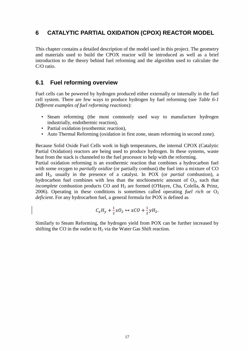
deficient. For any hydrocarbon fuel, a general formula for POX is defined as
.
Similarly to Steam Reforming, the hydrogen yield from POX can be further increased by
shifting the CO in the outlet to H2 via the Water Gas Shift reaction.
18
Table 6-1 Different examples of fuel reforming reactions (O’Hayre et al., 2006)
Reaction type Stoichiometric formula (kJ/mol)
Steam Reforming +165.2
Water-Gas Shift -41.2
Partial Oxidation -35.7
Partial Oxidation -319.1
Methane Combustion -880
Hydrogen Combustion -284
6.2 Calculating the C/O ratio
The CPOX reactor runs on oxygen from air and fuel. In this case it is a high hydrocarbon -
Dodecane C12H26 ( ). The catalytic reactor gets a fuel mix at the input.
Depending on the inlet stream flow of the air (input power of the blower) and fuel,
different carbon to oxygen ratios (C/O ratios) can be reached.
Table 6-2 Components of dry air, their volume percentages and molecular masses
(Wikipedia, 2008)
Components in Dry Air Volume percentage Molecular Mass
M [g/mol]
Nitrogen (N2) 78.09% 28.02
Oxygen (O2) 20.95% 32.00
Argon (Ar) 0.93% 39.94
Carbon dioxide (CO2) 0.03% 44.01
The air molar mass is calculated according to the formula
.
The fuel molar mass is the sum of molecular masses of carbon and hydrogen in the
Dodecane compound:
,
where and .
19
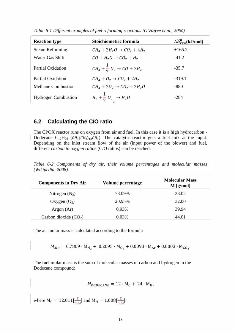
The C/O ratio is defined as the ratio of mole flow rates of carbon and oxygen in the inlet
streams:
,
where is a mass flow rate in [g/s]. A few examples of C/O ratio calculation are given in
Table 6-3 Numerical examples of C/O ratio calculation.
Table 6-3 Numerical examples of C/O ratio calculation
Fuel flow rate
[g/s]
Air flow
rate [g/s] [mol/s] [mol/s] C/O ratio
0.2708 1.444 1.59×10⁻³
4.98×10⁻²
0.1914
0.2572 1.444 1.51×10⁻³
4.98×10⁻²
0.1818
0.2843 1.444 1.67×10⁻³
4.98×10⁻²
0.2009
The spreadsheet example of C/O ratio calculation is available in APPENDIX B: Microsoft
Excel Implementations.
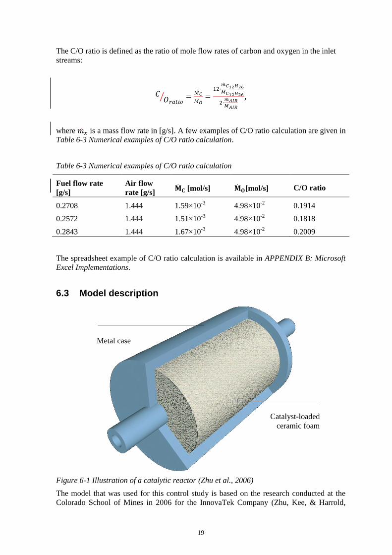
6.3 Model description
Figure 6-1 Illustration of a catalytic reactor (Zhu et al., 2006)
The model that was used for this control study is based on the research conducted at the
Colorado School of Mines in 2006 for the InnovaTek Company (Zhu, Kee, & Harrold,
Catalyst-loaded
ceramic foam
Metal case
20
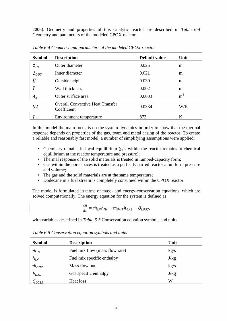
2006). Geometry and properties of this catalytic reactor are described in Table 6-4
Geometry and parameters of the modeled CPOX reactor.
Table 6-4 Geometry and parameters of the modeled CPOX reactor
Symbol Description Default value Unit
Outer diameter 0.025 m
Inner diameter 0.021 m
Outside height 0.030 m
Wall thickness 0.002 m
Outer surface area 0.0033 m2
Overall Convective Heat Transfer
Coefficient 0.0334 W/K
Environment temperature 873 K
In this model the main focus is on the system dynamics in order to show that the thermal
response depends on properties of the gas, foam and metal casing of the reactor. To create
a reliable and reasonably fast model, a number of simplifying assumptions were applied:
• Chemistry remains in local equilibrium (gas within the reactor remains at chemical
equilibrium at the reactor temperature and pressure);
• Thermal response of the solid materials is treated in lumped-capacity form;
• Gas within the pore spaces is treated as a perfectly stirred reactor at uniform pressure
and volume;
• The gas and the solid materials are at the same temperature;
• Dodecane in a fuel stream is completely consumed within the CPOX reactor.
The model is formulated in terms of mass- and energy-conservation equations, which are
solved computationally. The energy equation for the system is defined as
,
with variables described in Table 6-5 Conservation equation symbols and units.
Table 6-5 Conservation equation symbols and units
Symbol Description Unit
Fuel mix flow (mass flow rate) kg/s
Fuel mix specific enthalpy J/kg
Mass flow out kg/s
Gas specific enthalpy J/kg
Heat loss W
21
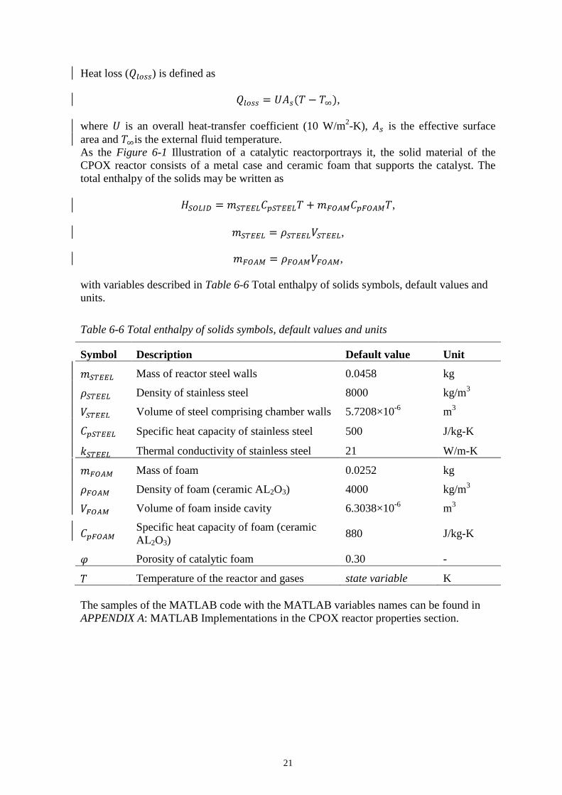
Heat loss ( ) is defined as
,
where is an overall heat-transfer coefficient (10 W/m2-K), is the effective surface
area and is the external fluid temperature.
As the Figure 6-1 Illustration of a catalytic reactorportrays it, the solid material of the
CPOX reactor consists of a metal case and ceramic foam that supports the catalyst. The
total enthalpy of the solids may be written as
,
,
,
with variables described in Table 6-6 Total enthalpy of solids symbols, default values and
units.
Table 6-6 Total enthalpy of solids symbols, default values and units
Symbol Description Default value Unit
Mass of reactor steel walls 0.0458 kg
Density of stainless steel 8000 kg/m3
Volume of steel comprising chamber walls 5.7208×10⁻⁶
m3
Specific heat capacity of stainless steel 500 J/kg-K
Thermal conductivity of stainless steel 21 W/m-K
Mass of foam 0.0252 kg
Density of foam (ceramic AL2O3) 4000 kg/m3
Volume of foam inside cavity 6.3038×10⁻⁶
m3
Specific heat capacity of foam (ceramic
AL2O3) 880 J/kg-K
Porosity of catalytic foam 0.30 -
Temperature of the reactor and gases state variable K
The samples of the MATLAB code with the MATLAB variables names can be found in
APPENDIX A: MATLAB Implementations in the CPOX reactor properties section.
22
7 DIFFERENTIAL ALGEBRAIC EQUATIONS
7.1 Theory behind DAEs
A differential equation is an equation that contains an unknown function and one or more
of its derivatives (Steward, 2008). In a DAE formulation it is not necessary to formulate
explicit equations for the time-derivatives of each state. Instead we can, for example,
formulate the conservation of energy.
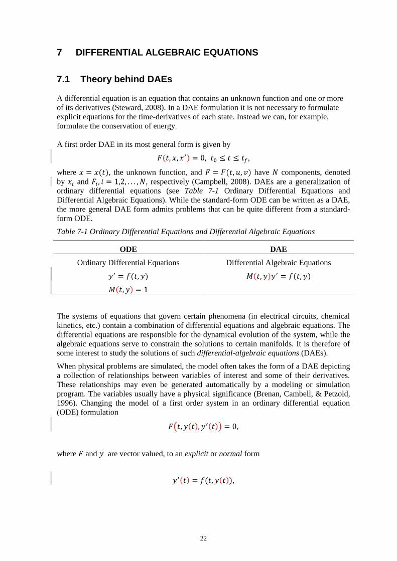
A first order DAE in its most general form is given by
,
where , the unknown function, and have components, denoted
by and , respectively (Campbell, 2008). DAEs are a generalization of
ordinary differential equations (see Table 7-1 Ordinary Differential Equations and
Differential Algebraic Equations). While the standard-form ODE can be written as a DAE,
the more general DAE form admits problems that can be quite different from a standard-
form ODE.
Table 7-1 Ordinary Differential Equations and Differential Algebraic Equations
ODE DAE
Ordinary Differential Equations Differential Algebraic Equations
The systems of equations that govern certain phenomena (in electrical circuits, chemical
kinetics, etc.) contain a combination of differential equations and algebraic equations. The
differential equations are responsible for the dynamical evolution of the system, while the
algebraic equations serve to constrain the solutions to certain manifolds. It is therefore of
some interest to study the solutions of such differential-algebraic equations (DAEs).
When physical problems are simulated, the model often takes the form of a DAE depicting
a collection of relationships between variables of interest and some of their derivatives.
These relationships may even be generated automatically by a modeling or simulation
program. The variables usually have a physical significance (Brenan, Cambell, & Petzold,
1996). Changing the model of a first order system in an ordinary differential equation
(ODE) formulation
,
where and are vector valued, to an explicit or normal form
,
23
may produce less meaningful variables. In the case of computer-generated or nonlinear
models, it may be time consuming or impossible to obtain an explicit model. Parameters
are present in many applications. Changing parameter values can alter the relationships
between variables and require different explicit models with solution manifolds of different
dimensions. If the original DAE can be solved directly, then it becomes easier for the
scientist or engineer to explore the effect of modeling changes and parameter variation. It
also becomes easier to interface modeling software directly with design software. These
advantages enable researchers to focus their attention on the physical problem of interest.
There are also numerical reasons for considering DAE‟a. The change to explicit form, even
if possible, can destroy sparsity and prevent the exploitation of system structure.
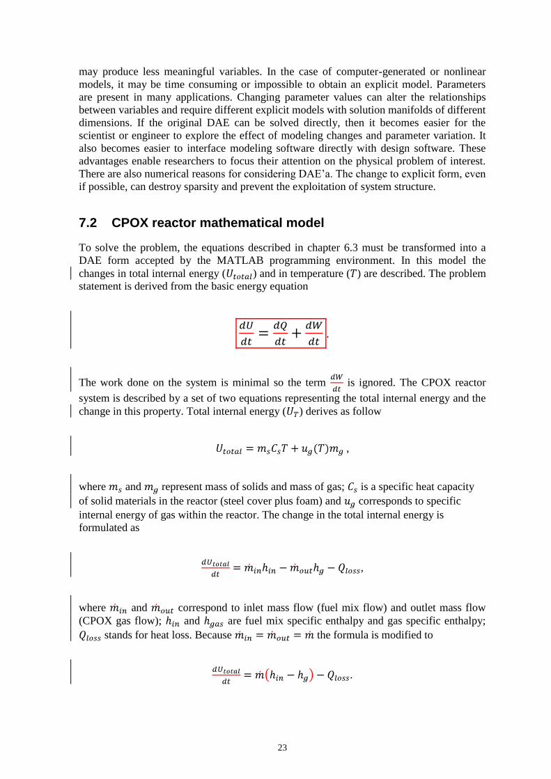
7.2 CPOX reactor mathematical model
To solve the problem, the equations described in chapter 6.3 must be transformed into a
DAE form accepted by the MATLAB programming environment. In this model the
changes in total internal energy ( ) and in temperature ( ) are described. The problem
statement is derived from the basic energy equation
.
The work done on the system is minimal so the term is ignored. The CPOX reactor
system is described by a set of two equations representing the total internal energy and the
change in this property. Total internal energy ( ) derives as follow
,
where and represent mass of solids and mass of gas; is a specific heat capacity
of solid materials in the reactor (steel cover plus foam) and corresponds to specific
internal energy of gas within the reactor. The change in the total internal energy is
formulated as
,
where and correspond to inlet mass flow (fuel mix flow) and outlet mass flow
(CPOX gas flow); and are fuel mix specific enthalpy and gas specific enthalpy;
stands for heat loss. Because the formula is modified to
.
24
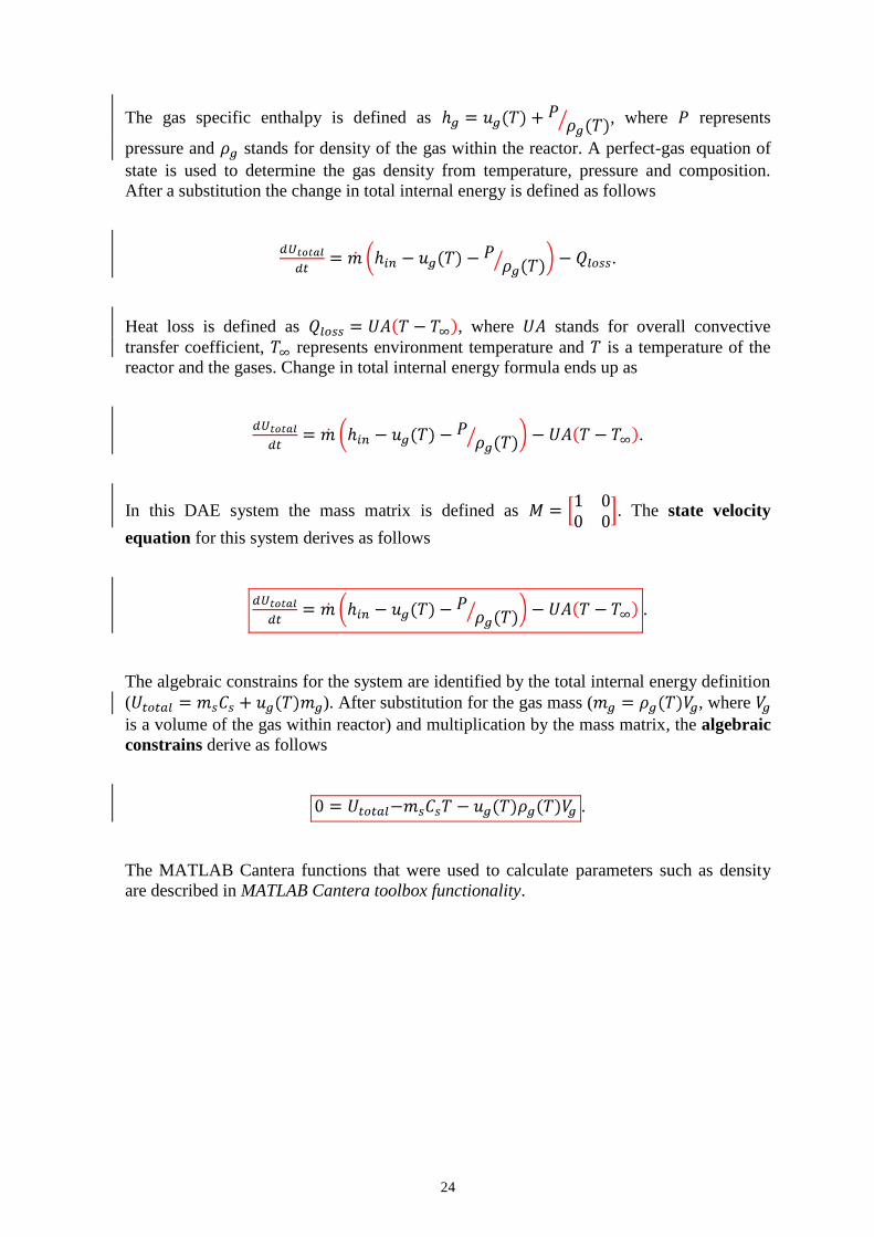
The gas specific enthalpy is defined as , where represents
pressure and stands for density of the gas within the reactor. A perfect-gas equation of
state is used to determine the gas density from temperature, pressure and composition.
After a substitution the change in total internal energy is defined as follows
.
Heat loss is defined as , where stands for overall convective
transfer coefficient, represents environment temperature and is a temperature of the
reactor and the gases. Change in total internal energy formula ends up as
.
In this DAE system the mass matrix is defined as . The state velocity
equation for this system derives as follows
.
The algebraic constrains for the system are identified by the total internal energy definition
( ). After substitution for the gas mass ( , where
is a volume of the gas within reactor) and multiplication by the mass matrix, the algebraic
constrains derive as follows
.
The MATLAB Cantera functions that were used to calculate parameters such as density
are described in MATLAB Cantera toolbox functionality.
25
8 MODEL TESTING
This chapter will present the results from the model. The model could not be validated
because the test-stand for this experiment is a work-in-progress at the Colorado Fuel Cell
Center.
The CPOX reactor problem is solved as initial value problem with consistent initial
conditions.
Initial Value Problem
In mathematics, including the field of differential equations, an initial value problem is an
ordinary differential equation together with the specified value, called the initial condition,
of the unknown function at a given point in the domain of the solution. In physics or other
sciences, modeling a system frequently amounts to solving an initial value problem; in this
context, the differential equation is an evolution equation specifying how, given initial
conditions, the system will evolve with time.
Consistent Initial Conditions
For an accurate solution, the consistent initial conditions need to be found. This will
guarantee that the solution to the initial value problem will be found.
Error longitude reduction
To make the calculations more precise, adjustments of the algebraic constrains were
applied. The solution for algebraic constrains is zero, so multiplying by any number will
not affect the result.
8.1 Implicit problem formulation (MATLAB fzero solution)
The implicit formulation of the CPOX reactor problem was solved using the MATLAB
fzero function (Zhu, Kee, & Harrold, 2006). An example of a heat-up transient can be
observed in Figure 8-1 Temperature history for an example CPOX heat-up transient.
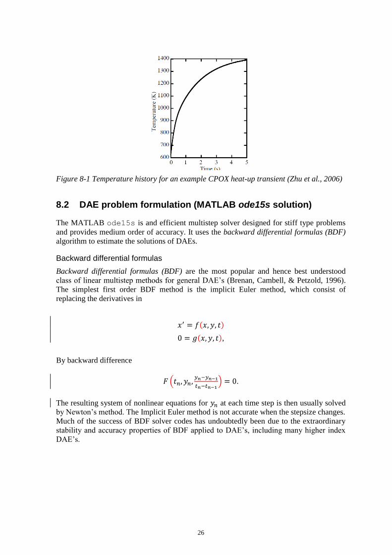
26
Figure 8-1 Temperature history for an example CPOX heat-up transient (Zhu et al., 2006)
8.2 DAE problem formulation (MATLAB ode15s solution)
The MATLAB ode15s is and efficient multistep solver designed for stiff type problems
and provides medium order of accuracy. It uses the backward differential formulas (BDF)
algorithm to estimate the solutions of DAEs.
Backward differential formulas
Backward differential formulas (BDF) are the most popular and hence best understood
class of linear multistep methods for general DAE‟s (Brenan, Cambell, & Petzold, 1996).
The simplest first order BDF method is the implicit Euler method, which consist of
replacing the derivatives in
,
By backward difference
.
The resulting system of nonlinear equations for at each time step is then usually solved
by Newton‟s method. The Implicit Euler method is not accurate when the stepsize changes.
Much of the success of BDF solver codes has undoubtedly been due to the extraordinary
stability and accuracy properties of BDF applied to DAE‟s, including many higher index
DAE‟s.
27
8.3 Model Results
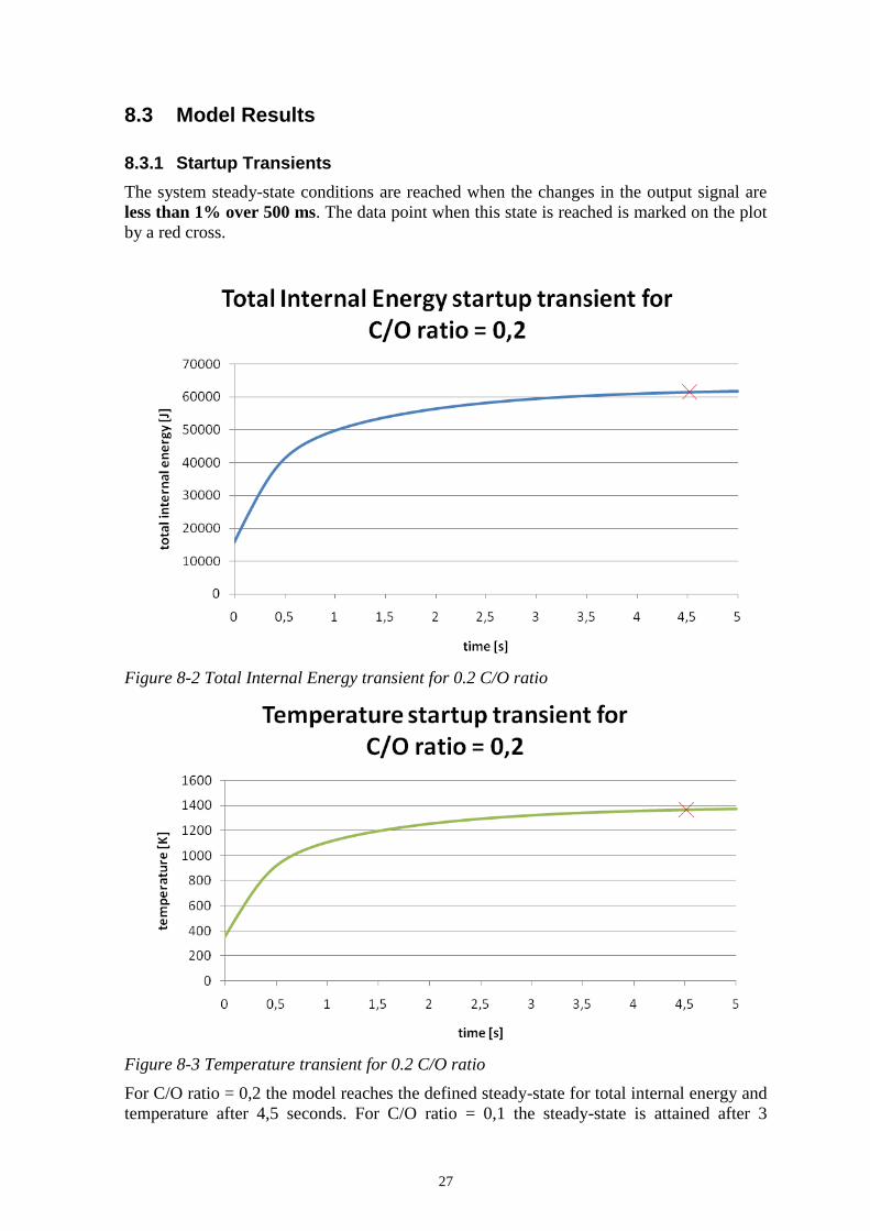
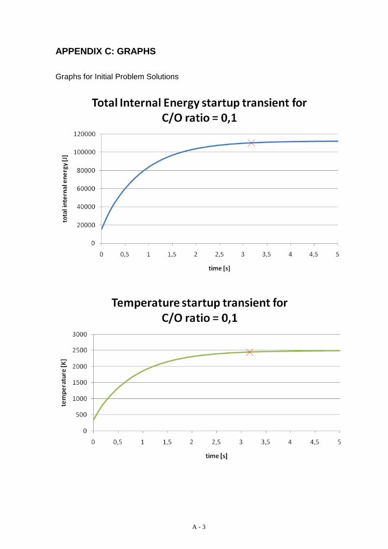
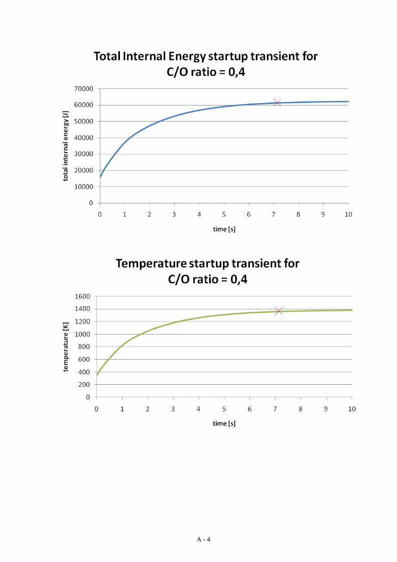
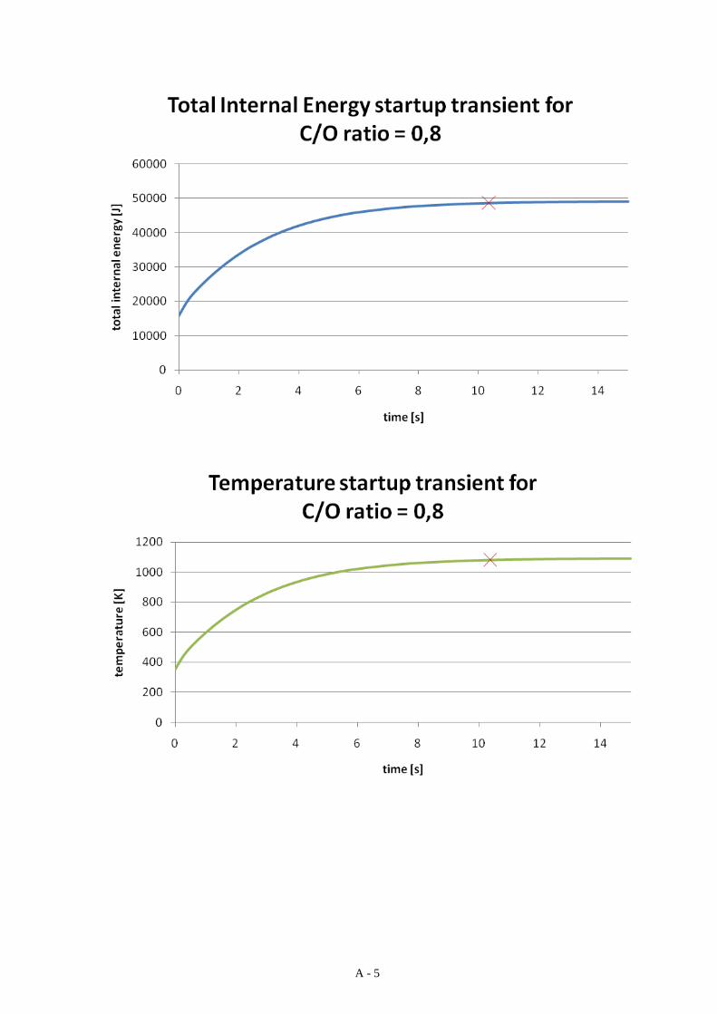
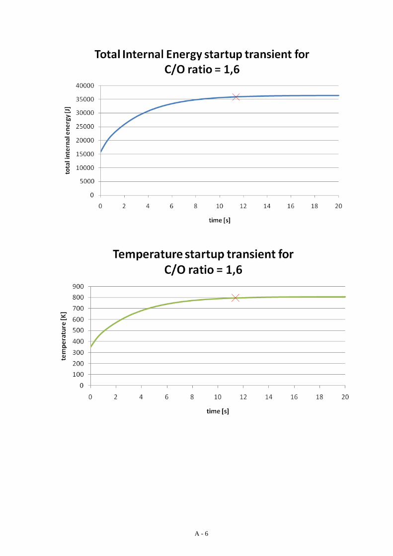
8.3.1 Startup Transients
The system steady-state conditions are reached when the changes in the output signal are
less than 1% over 500 ms. The data point when this state is reached is marked on the plot
by a red cross.
Figure 8-2 Total Internal Energy transient for 0.2 C/O ratio
Figure 8-3 Temperature transient for 0.2 C/O ratio
For C/O ratio = 0,2 the model reaches the defined steady-state for total internal energy and
temperature after 4,5 seconds. For C/O ratio = 0,1 the steady-state is attained after 3
28
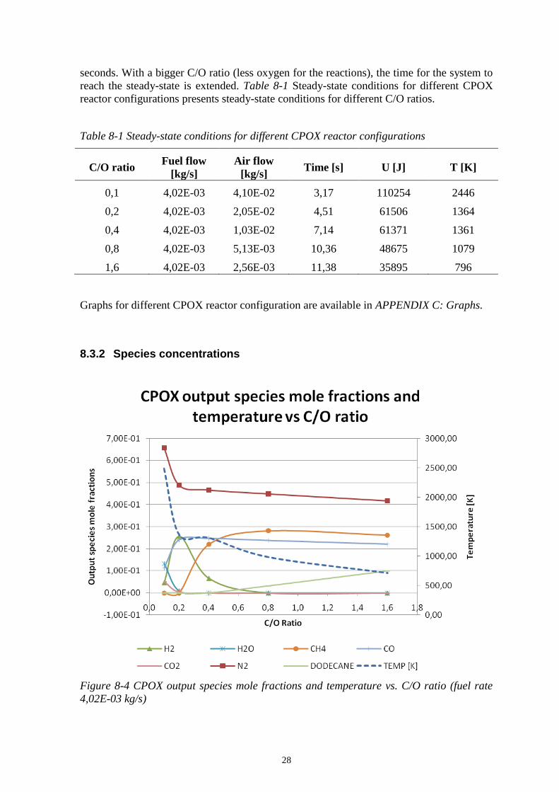
seconds. With a bigger C/O ratio (less oxygen for the reactions), the time for the system to
reach the steady-state is extended. Table 8-1 Steady-state conditions for different CPOX
reactor configurations presents steady-state conditions for different C/O ratios.
Table 8-1 Steady-state conditions for different CPOX reactor configurations
C/O ratio Fuel flow
[kg/s]
Air flow
[kg/s] Time [s] U [J] T [K]
0,1 4,02E-03 4,10E-02 3,17 110254 2446
0,2 4,02E-03 2,05E-02 4,51 61506 1364
0,4 4,02E-03 1,03E-02 7,14 61371 1361
0,8 4,02E-03 5,13E-03 10,36 48675 1079
1,6 4,02E-03 2,56E-03 11,38 35895 796
Graphs for different CPOX reactor configuration are available in APPENDIX C: Graphs.
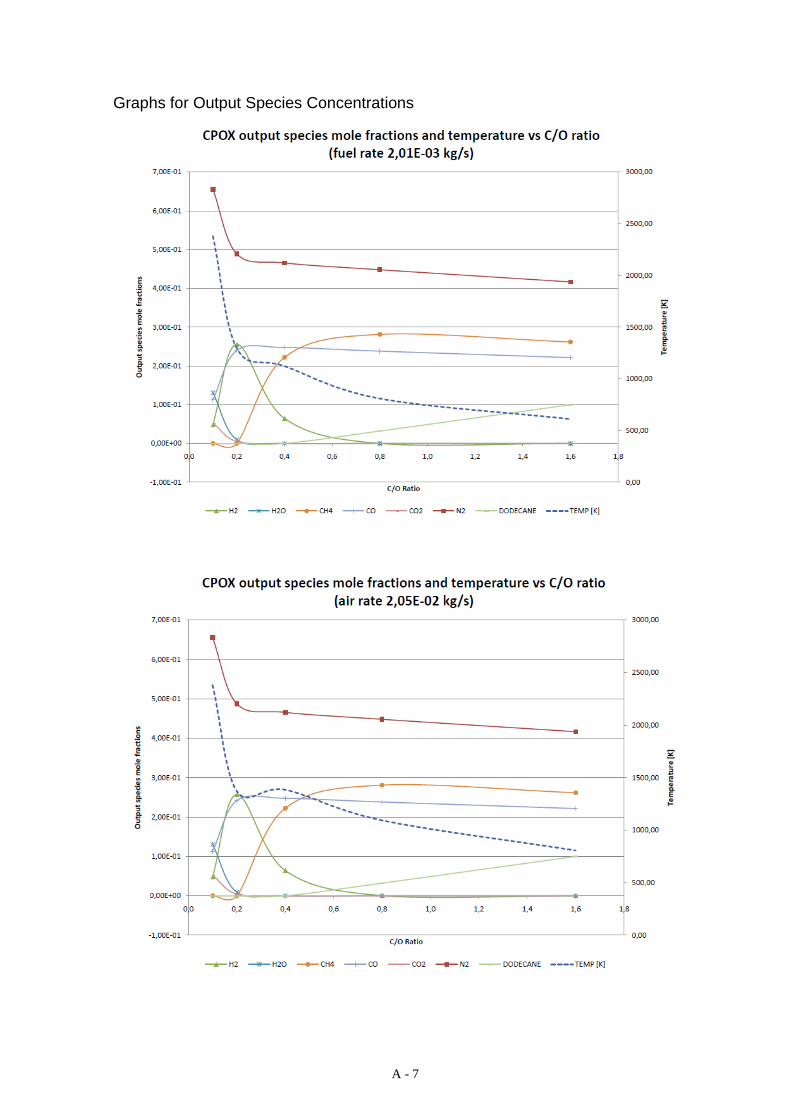
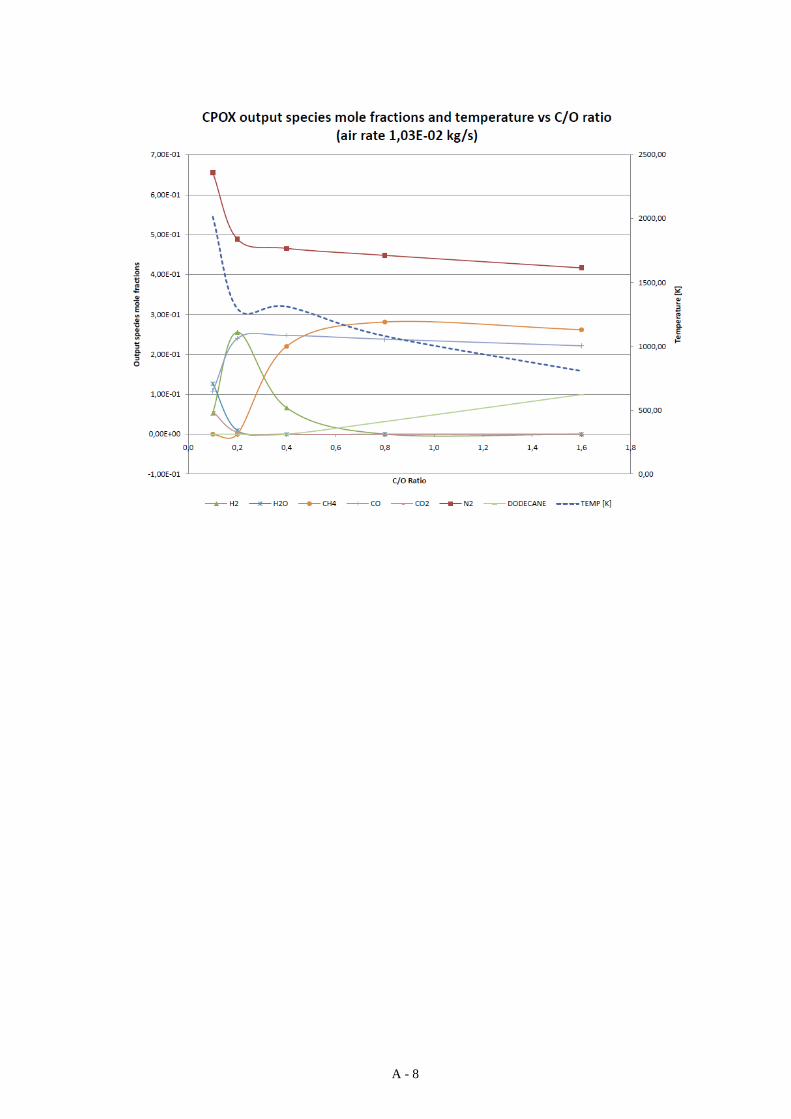
8.3.2 Species concentrations
Figure 8-4 CPOX output species mole fractions and temperature vs. C/O ratio (fuel rate
4,02E-03 kg/s)
29
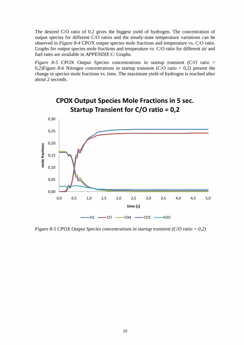
The desired C/O ratio of 0.2 gives the biggest yield of hydrogen. The concentration of
output species for different C/O ratios and the steady-state temperature variations can be
observed in Figure 8-4 CPOX output species mole fractions and temperature vs. C/O ratio.
Graphs for output species mole fractions and temperature vs. C/O ratio for different air and
fuel rates are available in APPENDIX C: Graphs.
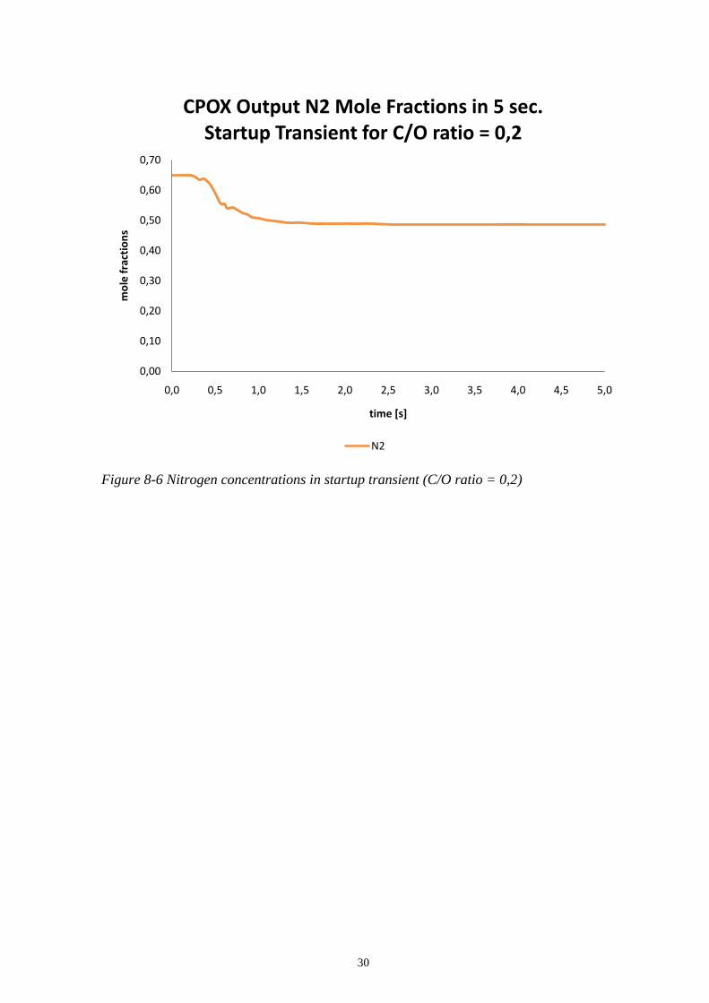
Figure 8-5 CPOX Output Species concentrations in startup transient (C/O ratio =
0,2)Figure 8-6 Nitrogen concentrations in startup transient (C/O ratio = 0,2) present the
change in species mole fractions vs. time. The maximum yield of hydrogen is reached after
about 2 seconds.
Figure 8-5 CPOX Output Species concentrations in startup transient (C/O ratio = 0,2)
0,00
0,05
0,10
0,15
0,20
0,25
0,30
0,0 0,5 1,0 1,5 2,0 2,5 3,0 3,5 4,0 4,5 5,0
mo
le f
ract
ion
s
time [s]
CPOX Output Species Mole Fractions in 5 sec. Startup Transient for C/O ratio = 0,2
H2 CO CH4 CO2 H2O
30
Figure 8-6 Nitrogen concentrations in startup transient (C/O ratio = 0,2)
0,00
0,10
0,20
0,30
0,40
0,50
0,60
0,70
0,0 0,5 1,0 1,5 2,0 2,5 3,0 3,5 4,0 4,5 5,0
mo
le f
ract
ion
s
time [s]
CPOX Output N2 Mole Fractions in 5 sec. Startup Transient for C/O ratio = 0,2
N2
31
9 FUTURE PROJECT DEVELOPMENT
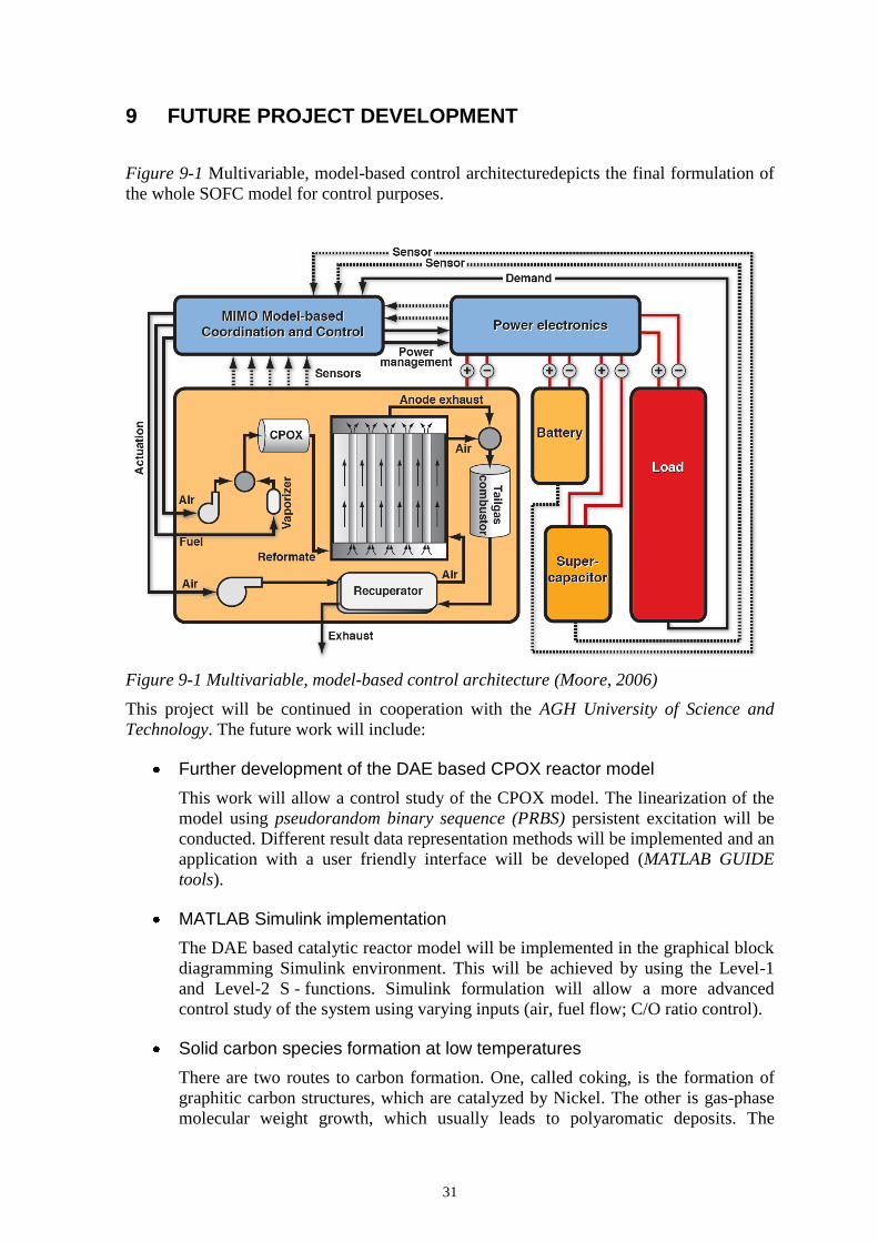
Figure 9-1 Multivariable, model-based control architecturedepicts the final formulation of
the whole SOFC model for control purposes.
Figure 9-1 Multivariable, model-based control architecture (Moore, 2006)
This project will be continued in cooperation with the AGH University of Science and
Technology. The future work will include:
Further development of the DAE based CPOX reactor model
This work will allow a control study of the CPOX model. The linearization of the
model using pseudorandom binary sequence (PRBS) persistent excitation will be
conducted. Different result data representation methods will be implemented and an
application with a user friendly interface will be developed (MATLAB GUIDE
tools).
MATLAB Simulink implementation
The DAE based catalytic reactor model will be implemented in the graphical block
diagramming Simulink environment. This will be achieved by using the Level-1
and Level-2 S - functions. Simulink formulation will allow a more advanced
control study of the system using varying inputs (air, fuel flow; C/O ratio control).
Solid carbon species formation at low temperatures
There are two routes to carbon formation. One, called coking, is the formation of
graphitic carbon structures, which are catalyzed by Nickel. The other is gas-phase
molecular weight growth, which usually leads to polyaromatic deposits. The
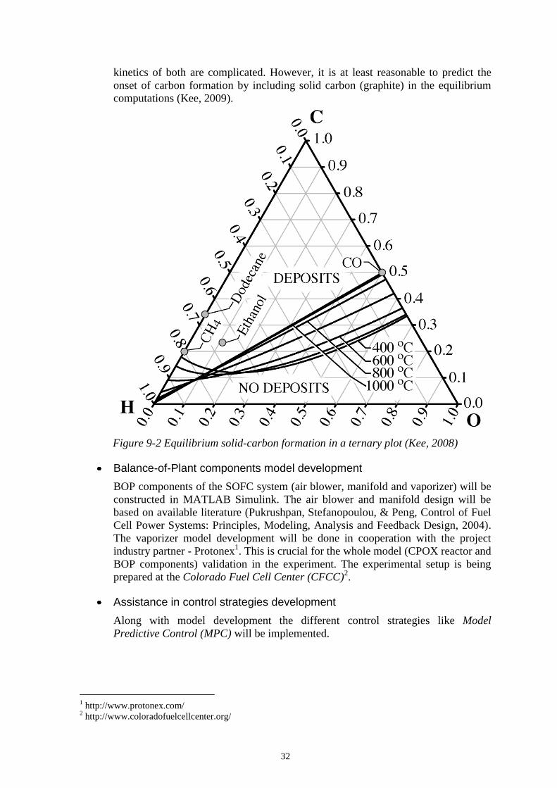
32
kinetics of both are complicated. However, it is at least reasonable to predict the
onset of carbon formation by including solid carbon (graphite) in the equilibrium
computations (Kee, 2009).
Figure 9-2 Equilibrium solid-carbon formation in a ternary plot (Kee, 2008)
Balance-of-Plant components model development
BOP components of the SOFC system (air blower, manifold and vaporizer) will be
constructed in MATLAB Simulink. The air blower and manifold design will be
based on available literature (Pukrushpan, Stefanopoulou, & Peng, Control of Fuel
Cell Power Systems: Principles, Modeling, Analysis and Feedback Design, 2004).
The vaporizer model development will be done in cooperation with the project
industry partner - Protonex1. This is crucial for the whole model (CPOX reactor and
BOP components) validation in the experiment. The experimental setup is being
prepared at the Colorado Fuel Cell Center (CFCC)2.
Assistance in control strategies development
Along with model development the different control strategies like Model
Predictive Control (MPC) will be implemented.
1 http://www.protonex.com/
2 http://www.coloradofuelcellcenter.org/
33
10 CONCLUSIONS
The correct C/O ratio is crucial for establishing optimal efficiency of a CPOX reactor and
the whole fuel cell system. As observed in Figure 8-4 CPOX output species mole fractions
and temperature vs. C/O ratio, control of this parameter will allow maximum hydrogen
yield at the C/O ratio of 0,2.
The results of this model are comparable to the work done by other research groups, as
presented in Section 8.1.
The analysis of the startup transient graphs proves that the speed of the transients is mostly
dependent on the input flow rates (the thermal mass of the reactor also has some
significance). This is an illustration of the non-linear behavior of the system. In a linear
system, the speed of the transients does not depend on the input magnitude (Vincent,
2009).
One reason for some inconsistencies might be the error handling mechanism in Cantera
and MATLAB. If error handling in those two environments do not match (one is coarse,
the other is fine) it might seriously influence the calculations. The error handling
mechanism in MATLAB is easy to check and adjust. Cantera is implemented in Python
and there is no direct error handling mechanism control from the MATLAB environment.
It is possible that an artifact of Cantera‟s error control can be observed at the Figure 8-5
CPOX Output Species concentrations in startup transient (C/O ratio = 0,2) in the small
signal disturbances at the beginning of the transient.
The next step of the project will focus on building the controller for the CPOX reactor.
Initial control will be on temperature. Thermal limitations of the CPOX reactor will be
considered. Because of carbonation issues the reactor is never operated at low temperatures
(below 1000°C).

35
REFERENCES
Brenan, K., Cambell, S., & Petzold, L. (1996). Numerical Solution of Initial-Value
Problems in Differential-Algebraic Equations. Philadelphia: Society for Industrial and
Applied Mathematics.
Campbell, S. L. (2008). Differential-algebraic equations. Retrieved January 3, 2009, from
Sholarpedia: http://www.scholarpedia.org/article/Differential-algebraic_equations
Carrette, L., Friedrich, K. A., & Stimming, U. (2001). Fuel Cells - Fundamentals and
Applications. Fuel Cells , 5-39.
Dorf, R. C., & Bishop, R. H. (2008). Modern Control Systems. Upper Saddle River, NJ:
Pearson Education, Inc.
Dvorak, D. (2008, April 21). Fuel Cell Operation. RES607: Fuel Cell Types and
Technologies . Akureyri, Iceland: RES | The School for Renewable Energy Science / The
University of Maine.
Dvorak, D. (2008, August 15). Introduction to Chemical Equilibrium. RES FC604:
Hydrogen Production and Storage Processes . Akureyri, Iceland: RES | The School for
Renewable Energy Science / The University of Maine.
EG&G Technical Services, Inc. (2004). Fuel Cell Handbook. Morgantown: U.S.
Department of Energy.
Jangsawang, W., Klimanek, A., & Gupta, K. A. (2006). Enhanced Yield of Hydrogen
From Wastes Using High Temperature Steam Gasification. Journal of Energy Resources
Technology , 179-185.
Journal of Physical and Chemical Reference Data. (2007, March 15). Retrieved January
15, 2009, from NIST Scientific and Technical Databases:
http://www.nist.gov/srd/jpcrd_28.htm
Kee, R., Rupley, F., & Miller, J. (2000). CHEMKIN Collection: EQUIL, Release 3.6. San
Diego: Reaction Design, Inc.
O'Hayre, R. P., Cha, S.-W., Colella, W., & Prinz, F. B. (2006). Fuel Cell Fundamentals.
New Jersey: John Wiley & Sons, Inc.
Pukrushpan, J. T., Peng, H., & Stefanopoulou, A. G. (2004). Control-Oriented Modeling
and Analysis for Automotive Fuel Cell Systems. Jurnal of Dynamic Systems,
Mesurements, and Control , 14-25.
Pukrushpan, J. T., Stefanopoulou, A. G., & Peng, H. (2004). Control of Fuel Cell Power
Systems: Principles, Modeling, Analysis and Feedback Design. London: Springer-Verlag.
Reynolds, W. C. (1986). The Element Potential Method for chemical equilibrium analysis:
implementation in the interactive program STANJAN (version 3). Stanford: Department of
Mechanical Engineering, Stanford University.
Romm, J. J. (2005). The Hype about Hydrogen. Washington: Island Press.

36
Smith, G. P., Golden, D. M., Frenklach, M., Moriarty, N. W., & Eiteneer, B. (n.d.). WHAT
IS GRI-Mech? Retrieved January 16, 2009, from GRI-Mech Project Overview:
http://www.me.berkeley.edu/gri_mech/overview.html
Steward, J. (2008). CALCULUS: Early Transcendentals. Belmont, CA: Thomson
Learning, Inc.
Wikipedia_Contributors. (2009, January 11). Chemical equilibrium. Retrieved January 14,
2009, from Wikipedia, The Free Encyclopedia:
http://en.wikipedia.org/w/index.php?title=Chemical_equilibrium&oldid=263338251
Wikipedia_Contributors. (2008, November 30). CHEMKIN. Retrieved January 19, 2009,
from Wikipedia, The Free Encyclopedia.:
http://en.wikipedia.org/w/index.php?title=CHEMKIN&oldid=254906051
Wikipedia_Contributors. (2009, January 11). Molar mass. Retrieved January 13, 2009,
from Wikipedia, The Free Encyclopedia.:
http://en.wikipedia.org/w/index.php?title=Molar_mass&oldid=263472805
Yucai, Z. (2001). Multivariable System Identification for Process Control. Eindhoven:
Elsevier Science & Technology Books.
Zhu, H., Kee, R. J., & Harrold, D. (2006). A model for the dynamic response of catalytic
reactor. Golden: Colorado School of Mines.
A - 1
APPENDIX A: MATLAB IMPLEMENTATIONS
MATLAB code listing is available as a PDF printout in the references directory
(references\ APPENDIX A - MATLAB code.pdf).
To get proper results with this DAE formulation, the vectorized option in the ode15s
solver needs to be turned off.
MATLAB Cantera toolbox functionality
A few of the functions available in MATLAB Cantera toolbox that were used to develop
the solution for this problem are described below. Brief help on each of those functions can
be displayed by typing
help (name of the function)
in the MATLAB environment.
Calculating the gas density
density(phase name)
Equilibrating
equilibrate(phase name, option)
There are few different ways the gas can be equilibrated:
'TP' - holding temperature and pressure fixed;
'UV' - fixed specific internal energy and specific volume;
'SV' - fixed specific entropy and specific volume;
'SP' - fixed specific entropy and pressure.
Obtaining the specific internal energy
intEnergy_mass(phase name)
Obtaining specific enthalpy
enthalpy_mass(phase name)
Displaying the molar concentrations of the species
moleFractions(phase name)
A - 2
APPENDIX B: Microsoft Excel Implementations
The C/O ratio calculations and the graphs depicting the output species concentration were
developed in Microsoft Excel worksheet.
The PDF printout of this worksheet is available in references directory:
references\APPENDIX B - 8 Hz CPOX Mdot Fuel Variation - C-O ratio.pdf
The MS Excel worksheets with the code to plot graphs for the startup transients and output
species concentrations are available in the references directory.
A - 3
APPENDIX C: GRAPHS
Graphs for Initial Problem Solutions
A - 4
A - 5
A - 6
A - 7
Graphs for Output Species Concentrations
A - 8

TH
E S
CH
OO
L F
O
R R E N E W A B L E E NE R
GY
SC
IE
NC
E
I C E L A N D
© 2009RES | the School for Renewable Energy Science, Iceland