soil structure interaction on spillway walls … · soil structure interaction on spillway walls...

U.S. Department of the Interior Bureau of Reclamation Technical Service Center Denver, Colorado September 2010

Report DSO-11-01

Soil Structure Interaction on Spillway Walls Adjacent to Embankments Dam Safety Technology Development Program

REPORT DOCUMENTATION PAGE Form Approved OMB No. 0704-0188

The public reporting burden for this collection of information is estimated to average 1 hour per response, including the time for reviewing instructions, searching existing data sources, gathering and maintaining the data needed, and completing and reviewing the collection of information. Send comments regarding this burden estimate or any other aspect of this collection of information, including suggestions for reducing the burden, to Department of Defense, Washington Headquarters Services, Directorate for Information Operations and Reports (0704-0188), 1215 Jefferson Davis Highway, Suite 1204, Arlington, VA 22202-4302. Respondents should be aware that notwithstanding any other provision of law, no person shall be subject to any penalty for failing to comply with a collection of information if it does not display a currently valid OMB control number. PLEASE DO NOT RETURN YOUR FORM TO THE ABOVE ADDRESS. 1. REPORT DATE (DD-MM-YYYY) 30-9-2010

2. REPORT TYPE Final

3. DATES COVERED (From - To)

4. TITLE AND SUBTITLE Soil Structure Interaction on Spillway Walls Adjacent to Embankments

5a. CONTRACT NUMBER 5b. GRANT NUMBER 5c. PROGRAM ELEMENT NUMBER

6. AUTHOR(S) Roman M. Koltuniuk, P.E., Bureau of Reclamation, Denver, Colorado, 86-68110

5d. PROJECT NUMBER 5e. TASK NUMBER 5f. WORK UNIT NUMBER

7. PERFORMING ORGANIZATION NAME(S) AND ADDRESS(ES) Bureau of Reclamation, Technical Services Center, Denver Federal Center, P.O. Box 25007, Denver, CO 80225

8. PERFORMING ORGANIZATION REPORT NUMBER DSO-11-01

9. SPONSORING/MONITORING AGENCY NAME(S) AND ADDRESS(ES) Bureau of Reclamation, Technical Services Center, Denver Federal Center, P.O. Box 25007, Denver, CO 80225

10. SPONSOR/MONITOR'S ACRONYM(S) 11. SPONSOR/MONITOR'S REPORT NUMBER(S) DSO-11-01

12. DISTRIBUTION/AVAILABILITY STATEMENT Available from National Technical Information Service, 5285 Port Royal Road, Springfield, VA 22161 13. SUPPLEMENTARY NOTES 14. ABSTRACT An extremely important aspect of the analyses of an embankment dam with a gated concrete spillway is the interaction of soil with the spillway walls during a seismic event. If the soil load becomes too great, the concrete spillway retaining wall may fail, opening up a large seepage path between the failed wall and the soil behind it, leading to erosion of the soil and, eventually, the entire dam. A more rigorous approach is required to evaluate seismic loads on concrete spillways other than traditional pseudostatic methods. This research will propose the use of the LSDYNA finite element code to model spillway walls with soil behind them in order to achieve this and will validate this code against results from centrifuge experiments at Berkeley . 15. SUBJECT TERMS Reclamation, soil-structure interaction, dynamic, static, spillway retaining walls, centrifuge, earthquake, LSDYNA finite element analysis, concrete 16. SECURITY CLASSIFICATION OF: 17. LIMITATION

OF ABSTRACT SAR

18. NUMBER OF PAGES

16

19a. NAME OF RESPONSIBLE PERSON Roman M. Koltuniuk, P.E.,

a. REPORT UL

b. ABSTRACT UL

a. THIS PAGE UL

19b. TELEPHONE NUMBER (Include area code 303-445-3225

Standard Form 298 (Rev. 8/98) Prescribed by ANSI Std. Z39.18

U.S. Department of the Interior Bureau of Reclamation Technical Service Center Structural Analysis Group, 86-68110 Denver, Colorado September 2010

Soil Structure Interaction on Spillway Walls Adjacent to Embankments Dam Safety Technology Development Program prepared by Roman Koltuniuk, P.E.

Mission Statements The mission of the Department of the Interior is to protect and provide access to our Nation’s natural and cultural heritage and honor our trust responsibilities to Indian Tribes and our commitments to island communities. The mission of the Bureau of Reclamation is to manage, develop, and protect water and related resources in an environmentally and economically sound manner in the interest of the American public.

iv

Contents

Page

Soil Structure Interaction..................................................................................... 1 Introduction ....................................................................................................... 1 Background ....................................................................................................... 1

Validation............................................................................................................... 3 Centrifuge Experiment ...................................................................................... 3 LSDYNA Finite Element Model ...................................................................... 4

Material Model 25 ....................................................................................... 4 Material Model 16 ....................................................................................... 6

Parametric Studies Using the LSDYNA Finite Element Model ....................... 8 Reverse Polarity of Seismic Record ........................................................... 8 Varying the Input Variables ........................................................................ 8 Varying the Wall Stiffness .......................................................................... 9 Varying the Wall Mass ............................................................................... 9

3-D Finite Element Example Model .................................................................... 9 Model Details .................................................................................................... 9

General ........................................................................................................ 9 Spillway Crest Structure ........................................................................... 10 Dam ........................................................................................................... 10 Foundation ................................................................................................ 10 Reservoir ................................................................................................... 10 Material Properties .................................................................................... 11

Upstream Zones 2 and 3 (Saturated SM) Material ............................. 11 Downstream Zones 2 and 3 (Dry SM) Material ................................. 11 Zone 1 (Saturated SC) Material .......................................................... 11 Underlying Overburden (Qal) Material .............................................. 11 Bedrock ............................................................................................... 11 Spillway Concrete ............................................................................... 12

Loads ............................................................................................................... 12 Results ............................................................................................................. 12

Base Line Time History Results ............................................................... 12 Varying the Wall Mass ............................................................................. 12 Varying the Wall Stiffness ........................................................................ 13 Varying the Damping ................................................................................ 13

Conclusions .......................................................................................................... 13 References ............................................................................................................ 15 Appendix A .......................................................................................................... 16

Soil Structure Interaction of Spillway Walls Adjacent to Embankments

1

Soil Structure Interaction

Introduction

An extremely important aspect of the analyses of an embankment dam with a gated concrete spillway is the interaction of soil with the spillway walls during a seismic event. If the soil load becomes too great, the concrete spillway retaining wall may fail, opening up a large seepage path between the failed wall and the soil behind it, leading to erosion of the soil and, eventually, the entire dam. This failure mode is significant and is associated with a large loss of life. Figure 1.1 shows a similar failure that occurred at Shi-Kang Dam in Taiwan. Although the embankment behind this failed retaining wall was not part of the main dam, if this had been part of an actual dam, it is very probable that a large breach would have occurred. Failure of the spillway pier, can fail the gates which is very undesirable, but results in lower consequences because the flow though the spillway is confined within the spillway walls and does not lead to embankment failure.

Background

The determination of seismic soil loads on retaining walls has traditionally been done using one of two pseudo static methods: Mononobe-Okabe or Woods. Mononobe-Okabe extends Coulomb’s theory of static active (and passive) earth pressures to include the effects of dynamic earth pressures on retaining walls. The Mononobe-Okabe theory incorporates the effect of earthquakes through the use of a constant horizontal acceleration in units of “g” acting on the soil mass comprising Coulomb’s active wedge (or passive wedge) within the backfill. The Mononobe-Okabe theory assumes that the wall movements are sufficient to fully mobilize the shear resistance along this backfill wedge, as is the case for Coulomb’s theory. To develop the dynamic active earth pressures, the wall movements are away from the backfill, while for the dynamic passive earth pressures, the wall movements are into the backfill. Wood’s theory assumes that the retaining wall has a non-yielding backfill behind it [1]. Sufficient wall movements do not occur and the shear strength of the backfill is not fully mobilized. Wood analyzed the response of a wall retaining non-yielding backfill to dynamic excitation assuming the soil backfill to be an elastic material. Wood’s simplified solutions showed that a static elastic solution for a uniform 1.0g horizontal acceleration gave very accurate results on the wall


2

under harmonic excitation of frequency f when dynamic amplification effects were negligible. This occurs when f/fs is less than about 0.5 where fs = Vs/4H is the cyclic frequency of the first shear mode of the backfill considered as a semi-infinite layer of depth H. Shaking table tests using dry sand backfill confirmed the applicability of Wood’s simplified solutions when the predominant frequency of shaking is significantly less than the fundamental frequency of the backfill. There have been no similar studies for saturated cohesive soils. The measured forces exceeded by a factor of 2 to 3 those predicted by the Mononobe-Okabe theory. Wood’s simplified solutions do not account for:

a) amplified accelerations from base to crest of the wall b) vertical or 2-component horizontal accelerations c) increase of modulus with depth in the backfill d) the out-of-phase response along the height of the wall between the

wall and soil at any given time e) the effect of the reduced soil stiffness with the level of shaking

induced in both the soil backfill and soil foundation Also, both of the above mentioned methods do not take into account the nonlinear behavior of soil during a seismic event, any three dimensional (3-D) effects around the spillway area, seismic motions in 3 orthogonal directions, and the complex nature of wave propagation produced with ground motion. Therefore, a more rigorous approach is required to evaluate seismic loads on concrete spillways. This Research Report will propose the use of the LSDYNA [2] finite element code in order to achieve this. This code has various soil material models available for use:

Material Model 16 incorporates the Mohr-Coulomb yield surface with a Tresca limit (response mode I). This model, combined with an equation-of-state, can be used to model soil structure interaction. Input parameters include density, shear modulus, Poisson’s ratio, tension cutoff, cohesion, pressure hardening coefficients, cohesion and pressure hardening coefficient at failure. Also, an equation-of-state that relates volumetric strain to pressure must be supplied.

Material Model 25 is an inviscid two invariant geologic cap model. The yield surface is defined by a failure envelope, a cap surface and a tension cutoff. The advantages of this model over other classical pressure-dependent plasticity models is the ability to control the amount of dilatency produced under shear loading and its ability to model plastic compaction. Input parameters include those obtained by fitting a curve through the failure data taken from a set of triaxial compression tests and parameters to define the cap hardening law, void fraction of an uncompressed sample and slope of the initial loading curve in hydrostatic compression.


3

Material Model 193 has a modified Drucker-Prager yield surface enabling the shape of the surface to be distorted into a more realistic definition for soils. Input parameters include density, shear modulus, Poisson’s ratio, friction angle, cohesion and dilation angle. The shear modulus, friction angle, cohesion and dilation angle can also be varied with depth of soil.

These nonlinear soil material models use the concepts and principles from the theory of plasticity. Total stresses are utilized where pore pressures are not explicitly taken into account. Total stress analysis is appropriate for cohesionless soils that are dry or very coarse and for most cohesive soils. For purposes of modeling core material against spillway walls, the soil above the phreatic surface can be modeled as dry, cohesionless material with a Mohr-Coulomb yield surface and an appropriate equation of state (relating volumetric strain versus pressure). The soil below the phreatic surface can be modeled as a cohesive material with no phi angle along with an equation of state that relates the volumetric strain versus pressure with a slope that is 3 to 4 times that of the bulk modulus of water.

Validation It is very important to validate any finite element results with experimental data. Professor Nicholas Sitar at the Department of Civil and Environmental Engineering, University of California, Berkeley measured accelerations and moments of earth retaining walls during seismic excitation in a centrifuge experiment as part of Linda Al Atik’s doctoral thesis [3]. The results of this work will be used to benchmark the performance of LSDYNA.

Centrifuge Experiment

The Berkeley centrifuge experiment consisted of two aluminum structures retaining Nevada Sand. The experiment configuration is shown in figure 2.1. The left aluminum structure is composed of stiff walls with a moment connection with the base while the right structure is composed of flexible walls with a similar base. The dimensions are shown in millimeters. LSDYNA will be used to model the Berkeley centrifuge experiment (in prototype scale) and will focus on comparing the accelerations in the soil and walls and the moments at the bottom of the inner stiff and flexible walls. The accelerations for this comparison are measured near the top of the soil and at the top of each wall. Figure 2.2 shows the location of the SG2 strain gage used to determine the wall


4

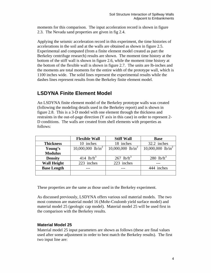
moments for this comparison. The input acceleration record is shown in figure 2.3. The Nevada sand properties are given in fig 2.4. Applying the seismic acceleration record in this experiment, the time histories of accelerations in the soil and at the walls are obtained as shown in figure 2.5. Experimental and computed (from a finite element model created as part the Berkeley centrifuge research) results are shown. The moment time history at the bottom of the stiff wall is shown in figure 2.6, while the moment time history at the bottom of the flexible wall is shown in figure 2.7. The units are lb-inches and the moments are total moments for the entire width of the prototype wall, which is 1100 inches wide. The solid lines represent the experimental results while the dashes lines represent results from the Berkeley finite element model.

LSDYNA Finite Element Model

An LSDYNA finite element model of the Berkeley prototype walls was created (following the modeling details used in the Berkeley report) and is shown in figure 2.8. This is a 3-D model with one element through the thickness and restraints in the out-of-page direction (Y axis in this case) in order to represent 2-D conditions. The walls are created from shell elements with properties as follows:

These properties are the same as those used in the Berkeley experiment. As discussed previously, LSDYNA offers various soil material models. The two most common are material model 16 (Mohr-Coulomb yield surface model) and material model 25 (geologic cap model). Material model 25 will be used first in the comparison with the Berkeley results.

Material Model 25 Material model 25 input parameters are shown as follows (these are final values used after some adjustment in order to best match the Berkeley results). The first two input line are:

Flexible Wall Stiff Wall Base Thickness 10 inches 18 inches 32.2 inches Young’s Modulus

10,000,000 lb/in2 10,000,000 lb/in2 10,000,000 lb/in2

Density 414 lb/ft3 267 lb/ft3 280 lb/ft3 Wall Height 223 inches 223 inches --- Base Length --- --- 444 inches


5

*MAT_GEOLOGIC_CAP_MODEL 25,0.000158,16700,7681,3.00,0.2700,3.00,0.085

Where : Mass density = 0.000158 slugs Bulk Modulus = 16,700 lb/in2 Shear Modulus = 7,681 lb/in2

Alpha = 3.00 Theta = 0.2700 Gamma = 3.00 Beta = 0.85

These last four variables are used to define a “Mohr-Coulomb” failure surface in the J1, (J2D) ½ space [2]. However, the easiest way to evaluate these variables is to test a one element material model 25 in triaxial compression and plot the Mohr circles for a variety of confining pressures and associated deviatoric pressures. This type of test was done using these variables and is shown in figure 2.9. This is a reasonable failure surface for Nevada sand. The next input line defines the cap and its movement with plastic strain [2]:

2.0,0.00005,0.150,13.00,0.000,0.000

Where : The shape of the cap = 2.00 Slope of the initial loading curve

in hydrostatic compression = 0.00005 The void fraction of an uncompressed sample = 0.15 Pressure at which the cap intersects the “Mohr-Coulomb” failure surface in the J1, (J2D) ½ space = 13.00 lb/in2

The next input line defines some plotting options and a tension cutoff:

3,2,1,0

Where :

Plot control variable = 3 (see LSDYNA users manual [2])


6

Formulation flag = 2 (see LSDYNA users manual [2]) Vectorization flag = 1 (see LSDYNA users manual [2]) Tension cutoff = 0 lb/in2

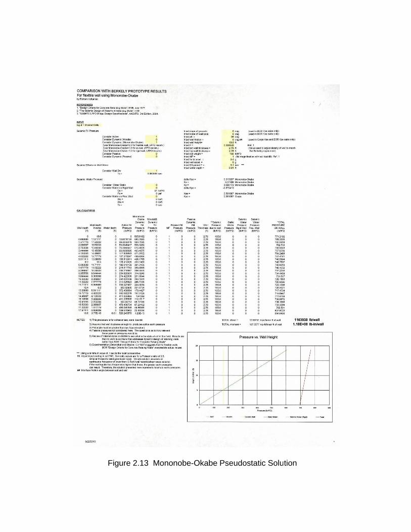
The hourglass control was chosen to be the standard Flanagan-Belytschko stiffness form with exact volume integration with all default parameters [2]. In LS-DYNA damping can be included through several mechanisms. There is inherent damping, which is the result of nonlinearities in the material models, contact surfaces, non-reflecting boundaries and so on. A user can also input damping in the form of Rayleigh damping (both mass and stiffness) and frequency range damping. Damping included by the user is termed “artificial damping.” Artificial damping is included if the finite element analysis shows signs of significant (or unrealistic) under-damped structural behavior. This under-damped behavior was observed in early runs of this model, therefore, a mass damping factor of 20.0 was applied to the soil and a mass damping factor of 3.0 was applied to the walls. The acceleration time histories at the top of the soil, at the top of the stiff wall and at the top of the flexible wall are shown in figure 2.10 and can be compared with the Berkeley results in figure 2.5. The time histories of the moments at the bottom of the flexible and stiff walls are shown in figures 2.11 and 2.12 respectively and can be compared to the Berkeley results in figures 2.6 and 2.7 respectively. As can be seen, the results are comparable. The accelerations are greater in the LSDYNA model, however, not significantly. The moment time histories compare well to the Berkeley results in terms of peak locations and shape of the curves. The LSDYNA analysis under predicts the static moment, peak values and residual increase in static post-earthquake moment for the flexible wall. However, for the stiff wall, LSDYNA over predicts the peak values during the seismic event and the static post-earthquake moment, while predicting static moment fairly well. Note there are significant differences between the experimental and computed time histories in the Berkeley results for the stiff wall. It is of interest to compare these results to Mononobe-Okabe and Woods pseudo-static solutions. Figure 2.13 shows the Mononobe-Okabe solution for the flexible wall resulting in a pseudo-static moment of 11.8 x 107 lb-in which can be compared to a peak in figure 2.11 of 3.0 x 107 lb-in. Figure 2.14 shows the Wood’s solution for the stiff wall resulting in a pseudostatic moment of 24.4 x 107 lb-in which can be compared to a peak in figure 2.12 of over 8.0 x 107 lb-in. This illustrates the conservative nature of the pseudo-static solutions.

Material Model 16 Material model 16 input parameters are shown as follows (these are final values used after some adjustment in order to best match the Berkeley results). The first four input lines are:


7

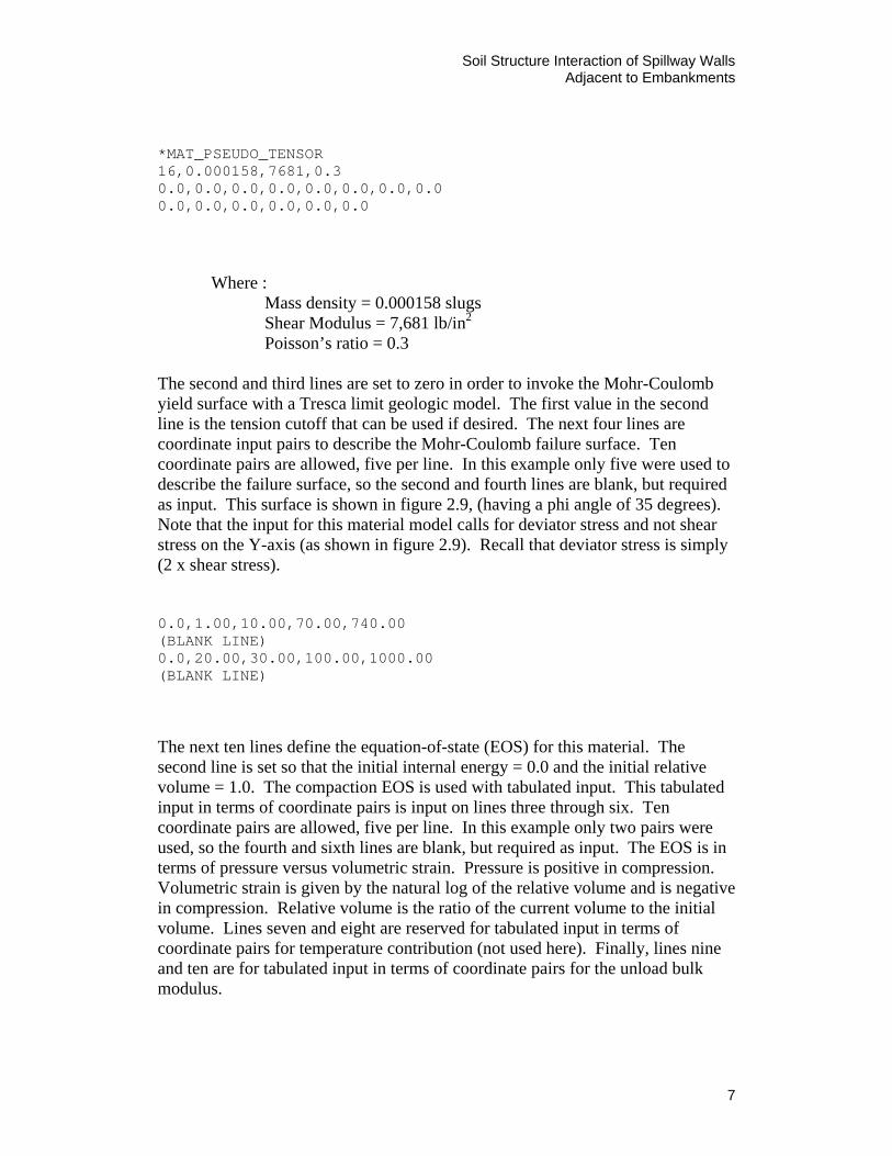
*MAT_PSEUDO_TENSOR 16,0.000158,7681,0.3 0.0,0.0,0.0,0.0,0.0,0.0,0.0,0.0 0.0,0.0,0.0,0.0,0.0,0.0

Where : Mass density = 0.000158 slugs Shear Modulus = 7,681 lb/in2 Poisson’s ratio = 0.3

The second and third lines are set to zero in order to invoke the Mohr-Coulomb yield surface with a Tresca limit geologic model. The first value in the second line is the tension cutoff that can be used if desired. The next four lines are coordinate input pairs to describe the Mohr-Coulomb failure surface. Ten coordinate pairs are allowed, five per line. In this example only five were used to describe the failure surface, so the second and fourth lines are blank, but required as input. This surface is shown in figure 2.9, (having a phi angle of 35 degrees). Note that the input for this material model calls for deviator stress and not shear stress on the Y-axis (as shown in figure 2.9). Recall that deviator stress is simply (2 x shear stress). 0.0,1.00,10.00,70.00,740.00 (BLANK LINE) 0.0,20.00,30.00,100.00,1000.00 (BLANK LINE) The next ten lines define the equation-of-state (EOS) for this material. The second line is set so that the initial internal energy = 0.0 and the initial relative volume = 1.0. The compaction EOS is used with tabulated input. This tabulated input in terms of coordinate pairs is input on lines three through six. Ten coordinate pairs are allowed, five per line. In this example only two pairs were used, so the fourth and sixth lines are blank, but required as input. The EOS is in terms of pressure versus volumetric strain. Pressure is positive in compression. Volumetric strain is given by the natural log of the relative volume and is negative in compression. Relative volume is the ratio of the current volume to the initial volume. Lines seven and eight are reserved for tabulated input in terms of coordinate pairs for temperature contribution (not used here). Finally, lines nine and ten are for tabulated input in terms of coordinate pairs for the unload bulk modulus.


8

*EOS_TABULATED_COMPACTION 16,0.0,0.0,1.0 0.0,-0.0008 (BLANK LINE) 0.0,10.00 (BLANK LINE) (BLANK LINE) (BLANK LINE) 16700.0,16700.0 (BLANK LINE) Hourglass control and damping are the same as described for material 25 above. The time histories of the moments at the bottom of the flexible and stiff walls are shown in figures 2.15 and 2.16 respectively and can be compared to the Berkeley results in figures 2.6 and 2.7 respectively. Again, the moment time histories compare well to the Berkeley results in terms of peak locations and shape of the curves. LSDYNA does a better job in predicting the moment time history response for the flexible wall in terms of peak moments and static post-earthquake moment using this material model as compared with material model 25. LSDYNA again over predicts the peaks for the stiff wall, however, does a better job in predicting the static post-earthquake moment, as compared with material model 25.

Parametric Studies Using the LSDYNA Finite Element Model

Some parametric studies using the LSDYNA model are presented here. Material 25 will be used for these studies.

Reverse Polarity of Seismic Record It is equally probable that a structure can be excited by a seismic event that is reversed in its polarity. Although, this was not done at Berkeley, the LSDYNA model was run with the seismic polarity reversed. (Actually, it is not clear which way the seismic record was applied at Berkeley.) The results are shown in figures 2.17 and 2.18 for the flexible and stiff wall respectively. Comparing with figures 2.11 and 2.12, one can see the significant differences in the shape of the response as well as in the peak values and the static post-earthquake moment. However, the general behavior is comparable. This illustrates the fact that seismic time histories should be applied with the polarity reversed and the most conservative response considered.

Varying the Input Variables Parametric studies were made for some of the input parameters. First, the cap was move out by increasing the pressure at which the cap intersects the “Mohr-Coulomb” failure surface in the J1, (J2D) ½ space from 13.00 lb/in2 to some large


9

pressure. The results were identical to those in figures 2.11 and 2.12, indicating that the cap was never reached in the run. Next, the last four variables are used to define a “Mohr-Coulomb” failure surface in the J1, (J2D) ½ space were moved upward in effect giving the sand some cohesion and a greater phi angle. This is not a realistic case, however, it was of interest to see the behavior. The result was the same shape time histories as shown in figures 2.11 and 2.12, however, the static post-earthquake moment was the same as the static moment. This would be expected confirming that the sand stayed in the linear range and did not touch any failure surface.

Varying the Wall Stiffness The wall stiffness was arbitrarily reduced by 2 times for both the stiff and the flexible walls. The moment time histories are shown in figures 2.19 and 2.20 (in gray) and are compared with the results using the reverse polarity seismic record (in black). As the stiffness decreases, the loading on the wall decreases. Statically, the load goes from an at-rest condition toward an active condition. Post-earthquake static loads are reduced even more significantly. The shapes of the time histories are in phase with the shapes of the time histories of the original stiff and flexible walls.

Varying the Wall Mass The wall mass of both the stiff and flexible walls was reduced arbitrarily by 10 times. The moment time histories are shown in figures 2.21 and 2.22 (in gray) and are compared with the results using the reverse polarity seismic record (in black). As can be seen, the response is reduced, as would be expected. The more mass a wall has the more it can contribute to the total moment response during a seismic event. The shapes of the time histories are comparable and in phase with the originals.

3-D Finite Element Example Model The effects of various parameters investigated in the previous section will be demonstrated using a 3-D model of an embankment dam with a spillway structure. Scoggins Dam was chosen for this purpose.

Model Details

General The TrueGrid [4] mesh generator was used to create the 3-D finite element model of the dam, the reservoir, the spillway crest structure and the surrounding


10

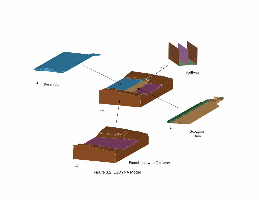
topography. LS-DYNA was used to analyze this model. The spillway crest structure was the focus of this analysis because it abuts to the core material of the dam and its failure during a seismic event could damage the continuous water barrier, resulting in a catastrophic release of the reservoir. A depiction of the entire model with dimensions is shown in figure 3.1. Figure 3.2 shows details of the various parts of the model. The model has 752172 nodes, 711605 brick elements and 2929 shell elements.

Spillway Crest Structure The spillway crest structure section modeled consists of wall panels supported by five counterforts. Figure 3.3 shows this crest structure section between station 8+48.25 and station 9+16.15. Figure 3.4 shows the reinforcement details of the counterforts. The spillway crest structure in the model consisted of the wall panels modeled using linear shell elements. The counterforts were modeled using linear beam elements attached to the shell elements. Each counterfort is represented with 28 beam elements. The moment of inertia, cross sectional area and density of the beam elements at any given elevation were adjusted to match that of the existing counterforts. Figure 3.5 shows the calculations for these values. Beam elements were also used underneath the spillway slab, connecting counterforts on either side, in order to help increase the stiffness of the slab, which in reality is connected to the rock (via cohesion and rock anchors as shown in Section A-A, figure 3.3) and is very stiff.

Dam The 3-D finite element model of the dam consists of various zoned materials as shown on figure 3.6 using solid elements with nonlinear soil properties. These zones were approximated in the finite element model as indicated by the colored sections. For the material properties input into the model for each of these zones, see Material Properties. Material 16 will be used as the material model for these zoned materials.

Foundation The 3-D finite element model of Scoggins Dam included the rock foundation using linear material solid elements. To properly model the seismic motions in the foundation, it is desirable to have at least 10 finite elements per seismic wavelength. The critical wavelength was determined by dividing the shear wave speed of the foundation rock (1,955 ft/s) by the assumed highest frequency of interest in the dam (a maximum frequency of 10 Hz). For this case, the wavelength is 195 ft, so an element size of 20 feet or less is needed. The element size beneath the dam is 20 feet or less.

Reservoir The reservoir behind the dam was modeled using solid elements with a fluid equation of state. Although the water in the spillway inlet was modeled, the gates and the interaction between the water and the gates were not modeled. This is because the loads from the gates to the spillway walls and piers are small


11

compared to the soil loads and concrete inertia. The reservoir was included upstream of the dam to account for global dam-to-water interaction that might affect displacement of the embankment dam, leading to movement of the soil in the vicinity of the spillway.

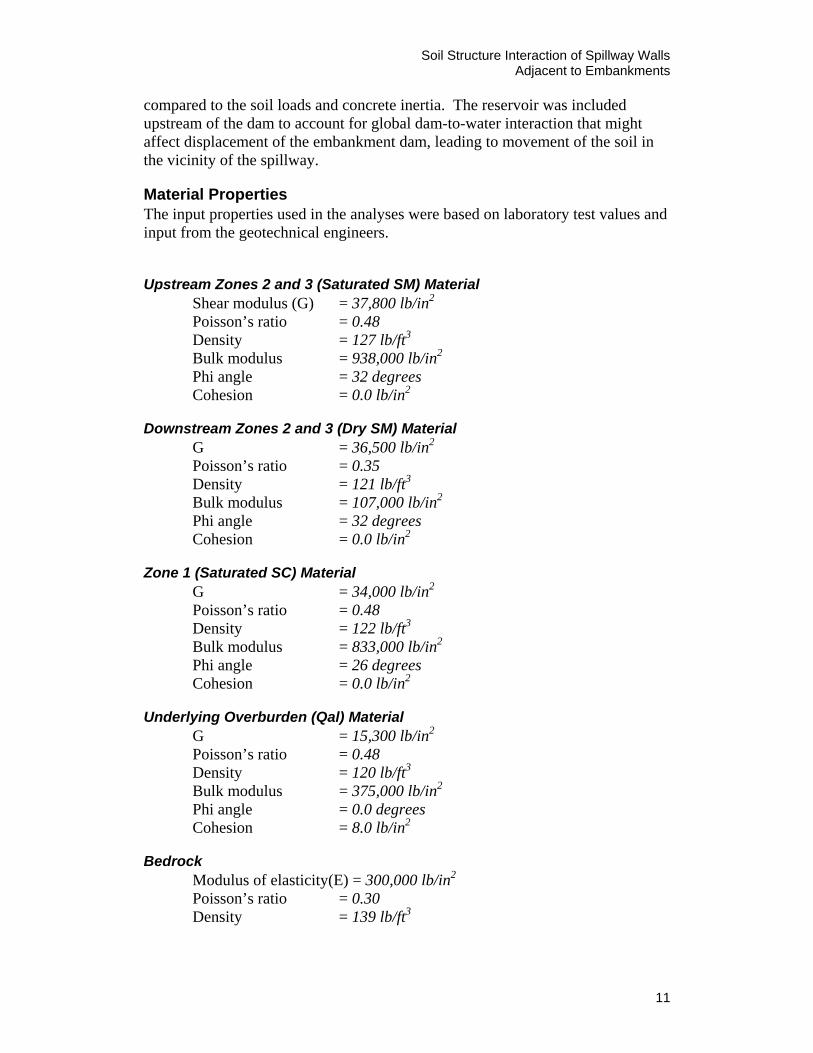
Material Properties The input properties used in the analyses were based on laboratory test values and input from the geotechnical engineers.

Upstream Zones 2 and 3 (Saturated SM) Material Shear modulus (G) = 37,800 lb/in2 Poisson’s ratio = 0.48 Density = 127 lb/ft3 Bulk modulus = 938,000 lb/in2 Phi angle = 32 degrees Cohesion = 0.0 lb/in2

Downstream Zones 2 and 3 (Dry SM) Material G = 36,500 lb/in2 Poisson’s ratio = 0.35 Density = 121 lb/ft3 Bulk modulus = 107,000 lb/in2 Phi angle = 32 degrees Cohesion = 0.0 lb/in2

Zone 1 (Saturated SC) Material G = 34,000 lb/in2 Poisson’s ratio = 0.48 Density = 122 lb/ft3 Bulk modulus = 833,000 lb/in2 Phi angle = 26 degrees Cohesion = 0.0 lb/in2

Underlying Overburden (Qal) Material G = 15,300 lb/in2 Poisson’s ratio = 0.48 Density = 120 lb/ft3 Bulk modulus = 375,000 lb/in2 Phi angle = 0.0 degrees Cohesion = 8.0 lb/in2

Bedrock Modulus of elasticity(E) = 300,000 lb/in2 Poisson’s ratio = 0.30 Density = 139 lb/ft3


12

Spillway Concrete Ec = 3,600,000 lb/in2 Poisson’s ratio = 0.16 Density = 150 lb/ft3

Loads

Static and dynamic loads were applied in LS-DYNA using load curves. Gravity loads were applied over 1.0 second and the model was allowed to reach a steady-state prior to application of the dynamic loads. Strong motion from the earthquake began after a few seconds into the computer runs. The finite element model was analyzed for a local GILR seismic event with a 50,000 year return period shown in figure 3.7. This motion was applied as 3 deconvolved orthogonal stress time histories at 0.01 second time step along a horizontal layer of element faces at depth of about 340 feet in the foundation and allowed to propagate up to the ground surface.

Results

The effects of the various parameters investigated for the Berkeley comparison studies will be compared in terms of moment and shear at the base of the middle counterfort (counterfort #3, figure 3.4). The base line case was run with all material properties as stated above and a global 3% damping applied to the entire model between 1.0 Hz and 10.0 Hz. An additional 10% stiffness damping was applied to the wall counterforts to dampen any high frequency vibrations.

Base Line Time History Results Figure 3.8 shows the moment time histories at the base of the middle counterfort. The time history plot for element 129 (red plot) is the moment for the middle counterfort on the embankment side wall, while the time history plot for element 274 (green plot) is the moment for the middle counterfort on the dam side wall. Figure 3.9 shows the shear time histories at the base of the same counterforts. The fact that the element 129 time histories are negative is just a sign convention in LSDYNA.

Varying the Wall Mass As with the centrifuge comparisons, the counterfort wall mass was reduced by ten times to see the effects on the moments and shears at the base of the middle counterfort. Figures 3.10 and 3.11 show the time histories of these moments and shears and can be compared to figures 3.8 and 3.9, respectively. As can be seen, the reduced mass decreases the ability of the wall to bend into the soil when it is being accelerated in that direction. This is evident in the fact that the time histories do not cross the Y-axis at zero (i.e. there is not sign change) during the


13

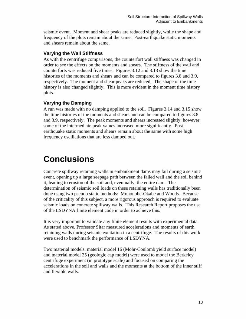
seismic event. Moment and shear peaks are reduced slightly, while the shape and frequency of the plots remain about the same. Post-earthquake static moments and shears remain about the same.

Varying the Wall Stiffness As with the centrifuge comparisons, the counterfort wall stiffness was changed in order to see the effects on the moments and shears. The stiffness of the wall and counterforts was reduced five times. Figures 3.12 and 3.13 show the time histories of the moments and shears and can be compared to figures 3.8 and 3.9, respectively. The moment and shear peaks are reduced. The shape of the time history is also changed slightly. This is more evident in the moment time history plots.

Varying the Damping A run was made with no damping applied to the soil. Figures 3.14 and 3.15 show the time histories of the moments and shears and can be compared to figures 3.8 and 3.9, respectively. The peak moments and shears increased slightly, however, some of the intermediate peak values increased more significantly. Post-earthquake static moments and shears remain about the same with some high frequency oscillations that are less damped out.

Conclusions Concrete spillway retaining walls in embankment dams may fail during a seismic event, opening up a large seepage path between the failed wall and the soil behind it, leading to erosion of the soil and, eventually, the entire dam. The determination of seismic soil loads on these retaining walls has traditionally been done using two pseudo static methods: Mononobe-Okabe and Woods. Because of the criticality of this subject, a more rigorous approach is required to evaluate seismic loads on concrete spillway walls. This Research Report proposes the use of the LSDYNA finite element code in order to achieve this. It is very important to validate any finite element results with experimental data. As stated above, Professor Sitar measured accelerations and moments of earth retaining walls during seismic excitation in a centrifuge. The results of this work were used to benchmark the performance of LSDYNA. Two material models, material model 16 (Mohr-Coulomb yield surface model) and material model 25 (geologic cap model) were used to model the Berkeley centrifuge experiment (in prototype scale) and focused on comparing the accelerations in the soil and walls and the moments at the bottom of the inner stiff and flexible walls.


14

In summary:

1) In general, LSDYNA predicted the acceleration of the soil and the walls well.

2) Deflection of the soil must be observed in order to spot and correct any signs of unreasonable hourglassing.

3) Using material model 25 (geologic cap model) LSDYNA under predicts the static moment, peak values and residual increase in static post-earthquake moment for the flexible wall. With material 16 (Mohr-Coulomb yield surface model), the peak values and residual increase in static post-earthquake moment are more in line with Berkeley results.

4) For the stiff wall, using material model 25, LSDYNA over predicts the peak values during the seismic event and the static post-earthquake moment, while predicting static moment fairly well. Using material model 16, LSDYNA again over predicts the peaks for the stiff wall, however, does a better job in predicting the static post-earthquake moment.

5) Large damping, characteristic of soil materials, must be employed in order to achieve reasonable results. This is also mentioned in the Berkeley results, where damping of 25% and greater was used depending on the shear strain of the soil.

Some parametric studies using LSDYNA were also done. Reducing the wall mass and wall stiffness reduced the peak moments and post-earthquake static moments, as would be expected. Reversing the polarity of the seismic record produced significant differences in the shape of the response as well as in the peak moment values and in the static post-earthquake moment. However, the general behavior is comparable. The effects of some of these parametric studies were also demonstrated using a 3-D model of an embankment dam with a spillway structure. Scoggins Dam was chosen for this purpose. The trends discussed above were also observed with this 3-D model. The LSDYNA finite element code appears to model the behavior of soil structure interaction on spillway walls during seismic excitation favorably. The shape and frequency of the response of the walls are within reason as compared with experimental results. Peak moments and post-earthquake moments also compare favorably. Further studies can always yield new insights. One can continue to adjust the material input parameters in order to try and obtain more accurate results. Static loads can be applied more rigorously through a layered approach. Updates will be made available as this new information is obtained.


15

References [1 ] Technical Report ITL-92-11, “The Seismic Design of Waterfront Retaining

Structures,” U.S Army Corps of Engineers, Washington, DC, November 1992.

[2] “LS-DYNA – Version 971,” Livermore Software Technology Corporation,

2876 Waverly Way, Livermore, CA 94551. [3 ] PEER Report 2008/104, “Experimental and Analytical Study of the Seismic

Performance of Retaining Structures,” Department of Civil and Environmental Engineering, University of California, Berkeley, March 2009.

[4] TrueGrid® Mesh Generator, XYZ Scientific Applications, Inc, Version 2.2,

Livermore, CA.


16

Appendix A

Figure 1.1 Coounterfort wall ffailure

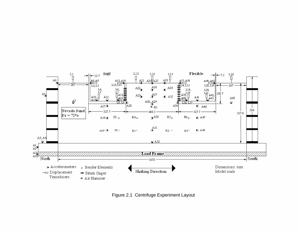
Figure 2.1 Centrifuge Experiment Layout

Figure 2.2 SG2 Strain Gage Location

Figure 2.3 Input Acceleration Record

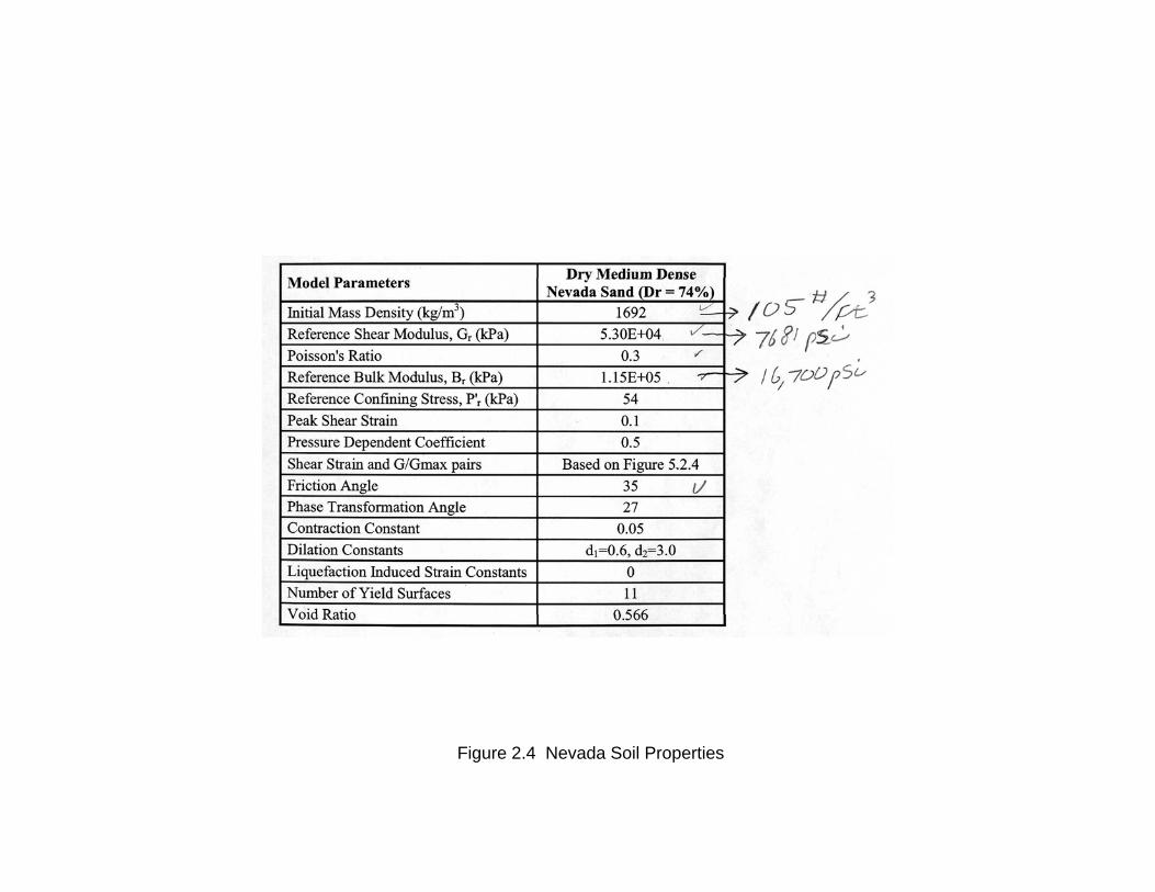
Figure 2.4 Nevada Soil Properties

Figure 2.5 Acceleratiion Time Historries

Figure 2.6 Moment Time History Near Bottom of Flexible Wall (SG2 Location)

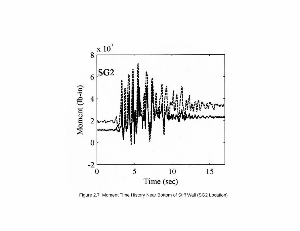
Figure 2.7 Moment Time History Near Bottom of Stiff Wall (SG2 Location)

Figure 2.8 LSDYNA Finite Element Model

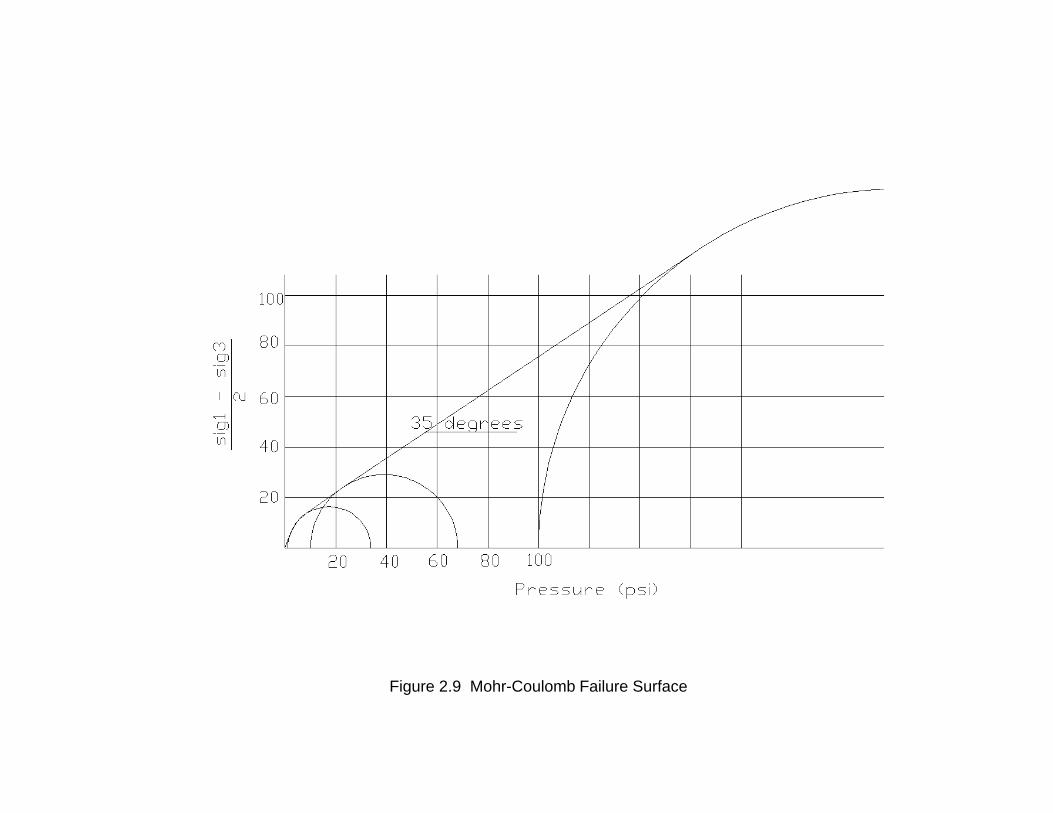
Figure 2.9 Mohr-Coulomb Failure Surface

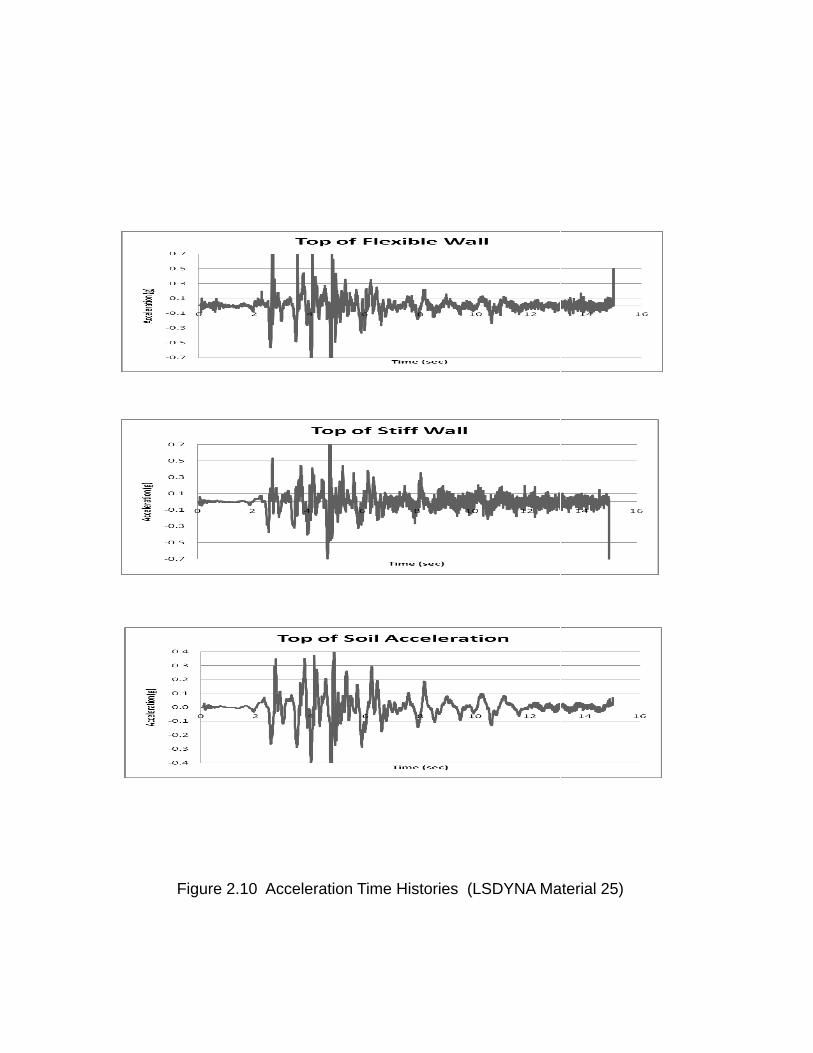
Figure 2.100 Acceleration Time Histories (LSDYNA Maaterial 25)

Figure 2.11 Moment Time History Near Bottom of Flexible Wall (LSDYNA Material 25)

Figure 2.12 Moment Time History Near Bottom of Stiff Wall (LSDYNA Material 25)

Figuree 2.13 Mononoobe-Okabe Pseeudostatic Solution

FFigure 2.14 Woood’s Pseudosstatic Solution

Figure 2.15 Moment Time History Near Bottom of Flexible Wall (LSDYNA Material 16)

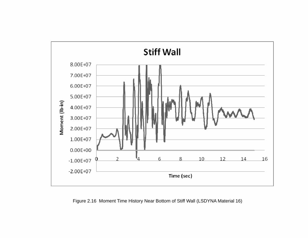
Figure 2.16 Moment Time History Near Bottom of Stiff Wall (LSDYNA Material 16)

Figure 2.17 Moment Time History Near Bottom of Flexible Wall (Reverse Earthquake Motion)

Figure 2.18 Moment Time History Near Bottom of Stiff Wall (Reverse Earthquake Motion)

Figure 2.19 Moment Time History Near Bottom of Flexible Wall (with 1/2 E)

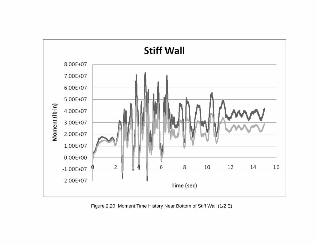
Figure 2.20 Moment Time History Near Bottom of Stiff Wall (1/2 E)

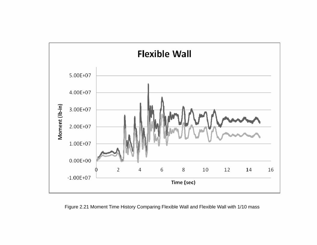
Figure 2.21 Moment Time History Comparing Flexible Wall and Flexible Wall with 1/10 mass

Figure 2.22 Moment Time History Comparing Stiff Wall and Stiff Wall with 1/10 mass

4,100 feetApplication of time history

2,070 feet

time history at100 feet abovebottom of model

Figure 3.1 LSDYNA model

Reservoir

Spillway

Scoggins Dam

Foundation with Qal layer

Figure 3.2 LSDYNA Model

Foundation with Qal layer

Figure 3.3 Spillway drawing

Counterfort #1Counterfort #4

Counterfort #2 Counterfort #3 Counterfort #5

Figure 3.4 Spillway drawing

Fi 3 5 S ill ll tiFigure 3.5 Spillway wall properties

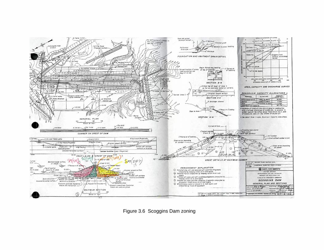
Figure 3.6 Scoggins Dam zoning

Figure 3.7 550K GILR free field

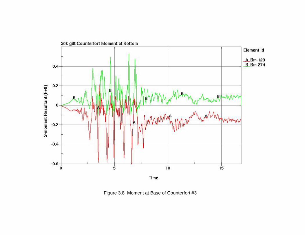
Fi 3 8 M t t B f C t f t #3Figure 3.8 Moment at Base of Counterfort #3

Fi 3 9 Sh t B f C t f t #3Figure 3.9 Shear at Base of Counterfort #3

Fi 3 10 M t t B f C t f t #3 (1/10 W ll M )Figure 3.10 Moment at Base of Counterfort #3 (1/10 Wall Mass)

Fi 3 11 Sh t B f C t f t #3 (1/10 W ll M )Figure 3.11 Shear at Base of Counterfort #3 (1/10 Wall Mass)

Fi 3 12 M t t B f C t f t #3 (1/5 W ll Stiff )Figure 3.12 Moment at Base of Counterfort #3 (1/5 Wall Stiffness)

Fi 3 13 Sh t B f C t f t #3 (1/5 W ll Stiff )Figure 3.13 Shear at Base of Counterfort #3 (1/5 Wall Stiffness)

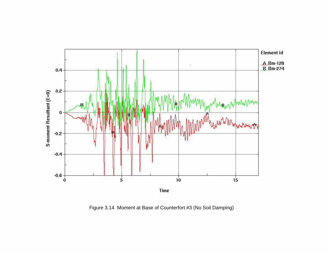
Fi 3 14 M t t B f C t f t #3 (N S il D i )Figure 3.14 Moment at Base of Counterfort #3 (No Soil Damping)

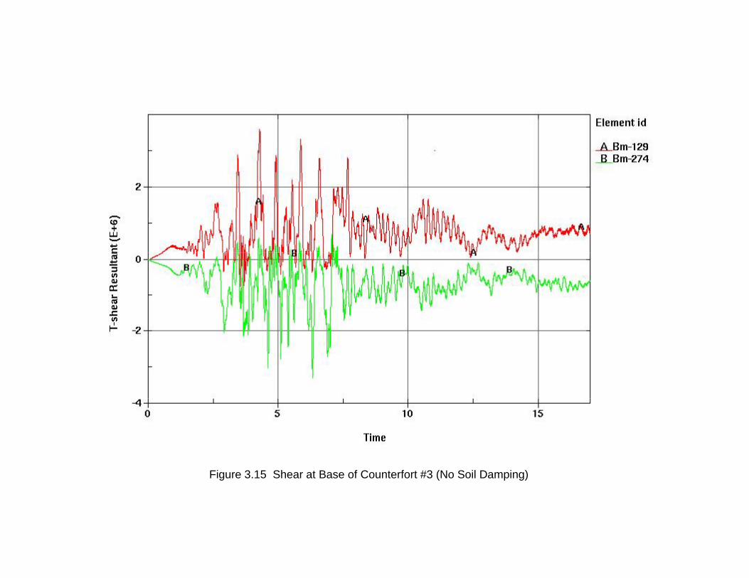
Fi 3 15 Sh t B f C t f t #3 (N S il D i )Figure 3.15 Shear at Base of Counterfort #3 (No Soil Damping)

soil structure interaction on spillway walls … · soil structure interaction on spillway walls...

Documents