soil spatial sssaj

Rep

rodu

ced

from

Soi

l Sci

ence

Soc

iety

of A

mer

ica

Jour

nal.

Pub

lishe

d by

Soi

l Sci

ence

Soc

iety

of A

mer

ica.

All

copy

right

s re

serv

ed.

Spatial Variability Analysis of Soil Physical Properties of Alluvial Soils

Javed Iqbal,* John A. Thomasson, Johnie N. Jenkins, Phillip R. Owens, and Frank D. Whisler

ABSTRACT ited on sandy or on loamy sediments. Therefore, it isimportant to study not only the extent of surface spatialAnalysis and interpretation of spatial variability of soils is a key-variability, but also the distribution of subsurface andstone in site-specific farming. Soil survey maps may have up to 0.41-

ha inclusions of dissimilar soils within a mapping unit. The objectives deep soil horizons.of this study were to determine the degree of spatial variability of soil Among the various soil physical properties, Ks andphysical properties and variance structure, and to model the sampling related measures are reported to have the highest statis-interval of alluvial floodplain soils. Soil profiles (n � 209) from 18 tical variability (Biggar and Nielsen, 1976). Boumaparallel transects were sampled with a mean separation distance of (1973) stressed the need for more studies on field vari-79.4 m. Each profile was classified into surface, subsurface, and deep ability of Ks and soil water retention curves. Stocktonhorizons. Structural analysis of soil bulk density (�b), sand, clay, satu-

and Warrick (1971) indicated that variability in Ks israted hydraulic conductivity (Ks), volumetric water content (�v) atboth a function of soil depth and position in the land-seven pressure potentials (�a) (�1, �10, �33, �67, �100, �500, andscape, as well as experimental errors in measuring Ks.�1500 kPa) were modeled for the three horizons. Variance of soilCameron (1978) sampled clay loam soils at six depthsphysical properties varied from as low as 0.01% (�b) to as high as

1542% (Ks). The LSD test indicated significant (P � 0.05) differences from five grid-sampled locations in a 225-m2 plot. Hein sand, clay, �b, Ks, and �v at various �a. Geostatistical analyses used the desorption method to determine soil waterillustrated that the spatially dependent stochastic component was pre- retention curves at pressure heads ranging from �10 todominant over the nugget effect. Structured semivariogram functions �500 kPa to calculate Ks. He found no consistent trendof each variable were used in generating fine-scale kriged contour across sampling depths in pressure head values frommaps. Overall autocorrelation, Moran’s I, indicated a 400-m sampling

�10 to �500 kPa, but the shape and magnitude of therange would be adequate for detection of spatial structure of sand,

average water retention curve differed among locations.silt, clay, and a 100-m sampling range for soil hydraulic propertiesHe further reported that the coefficient of variation ofand �b. The magnitude and spatial patterns soil physical propertysoil water content ranged from 4.3 to 13% in the surfacevariability have implications for variable rate applications and designlayer and from 2.4 to 6.5% in the deeper layers. In aof soil sampling strategies in alluvial floodplain soils.study of spatial variability in soil hydraulic properties,Vieira et al. (1981) used variogram, kriging, and co-kriging techniques to determine the magnitude of spatialSpatial variability of soil physical properties withinvariation and reported a range of 50 m for 1280 fieldor among agricultural fields is inherent in naturemeasured infiltration rates. Vauclin et al. (1983) sam-due to geologic and pedologic soil forming factors, butpled within a 70- by 40-m area at the nodes of a 10-msome of the variability may be induced by tillage andsquare grid and used classical and geostatistical tech-other management practices. These factors interact withniques to study spatial variability of sand, silt, and clayeach other across spatial and temporal scales, and arecontents, available water content (AWC), and waterfurther modified locally by erosion and depositionstored at �33 kPa. The strongest correlation was foundprocesses. Soils in the Mississippi Delta are alluvial inbetween sand content and AWC (r � �0.83) and thenature, originating from different soils, rocks, and un-cross variogram demonstrated that sand content wasconsolidated sediments in 24 states from Montana tospatially correlated with soil water content at �33 kPaPennsylvania, and deposited by the Mississippi and Ohiowithin a distance of ≈30 m and with AWC within aRivers and their tributaries (Logan, 1916). The stratifi-distance of ≈43 m. Sobieraj et al. (2003) found no spatialcation of different sediments deposited on top of eachstructure in Ks at distances � 25 m. Heiskanen andother spatially vary, for example, sandy sediments onMakitalo (2002) reported a range of 44 and 100 m fortop of clays or at other locations clay sediments depos-the water content and air-filled porosity at �a � �10kPa. Campbell (1978) reported sand content semivario-

J. Iqbal, Dep. of Agricultural and Biological Engineering, and F.D. gram ranges of 30 and 40 m for two different soil types.Whisler, Dep. of Plant and Soil Sci., Mississippi State Univ., and J.N.In summary, it is evident from the above studies thatJenkins, USDA-ARS, Crop Science Research Lab., P.O. Box 5367,

Mississippi State, MS 39762; J.A. Thomasson, Dep. of Agricultural spatial variability of various soil physical properties areand Biological Engineering, Texas A&M University, College Station, scale-dependent, especially the water transport proper-TX 77843; P.R. Owens, Dep. of Agronomy, Lilly Hall of Life Sci., ties of soils; therefore, it is a prerequisite to quantify the915 W. State Street, Purdue Univ., West Lafayette, IN 47907. This

spatial variability of soils before designing site-specificstudy was in part supported by The National Aeronautical and Spaceapplications like variable rate irrigation (VRI), seedAdministration funded Remote Sensing Technology Center at Missis-

sippi State University. Received 3 May 2004. *Corresponding author rate, fertilizer rate, and strategies for future soil sam-([email protected]). pling, especially for alluvial floodplain soils. The objec-Published in Soil Sci. Soc. Am. J. 69:�–� (2005).Soil & Water Management & Conservation Abbreviations: �v, volumetric water content; �b, soil bulk density; �a,

pressure potential; AWC, available water content; FC, field capacity;doi:10.2136/sssaj2004.0154© Soil Science Society of America Ks, saturated hydraulic conductivity; OM, organic matter; VRI, vari-

able rate irrigation; WP, wilting point.677 S. Segoe Rd., Madison, WI 53711 USA

1

Rep

rodu

ced

from

Soi

l Sci

ence

Soc

iety

of A

mer

ica

Jour

nal.

Pub

lishe

d by

Soi

l Sci

ence

Soc

iety

of A

mer

ica.

All

copy

right

s re

serv

ed.

2 SOIL SCI. SOC. AM. J., VOL. 69, �–� 2005

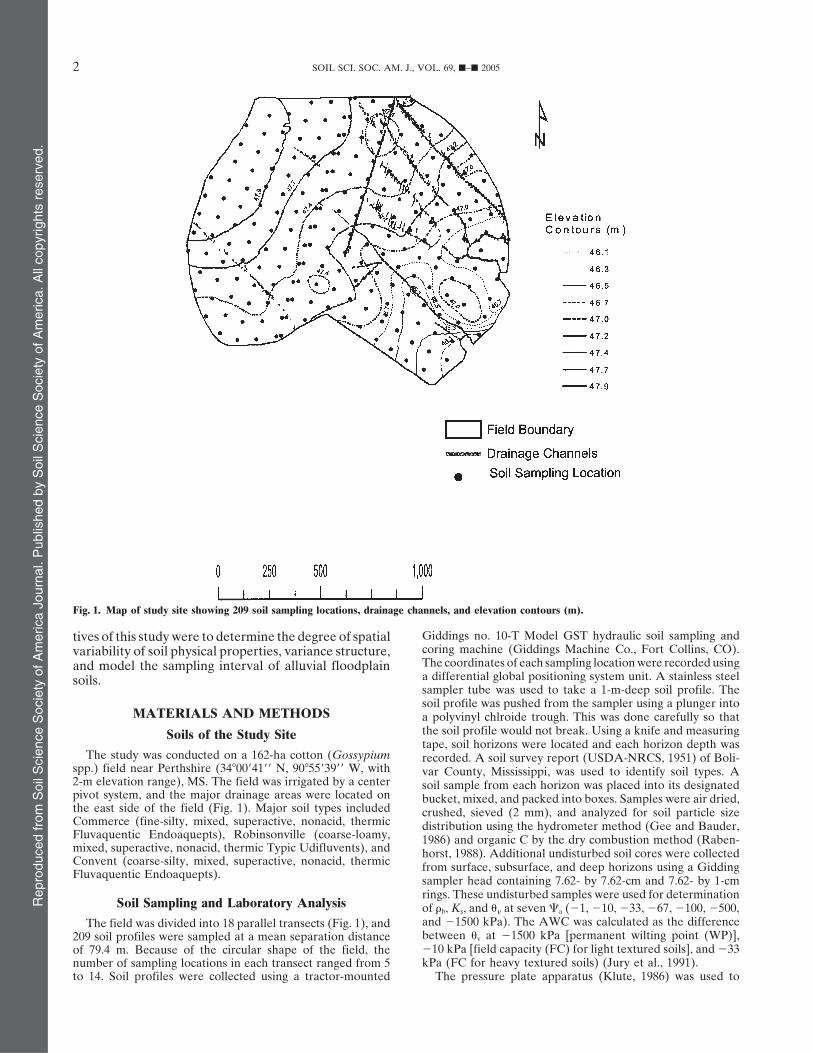
Fig. 1. Map of study site showing 209 soil sampling locations, drainage channels, and elevation contours (m).

Giddings no. 10-T Model GST hydraulic soil sampling andtives of this study were to determine the degree of spatialcoring machine (Giddings Machine Co., Fort Collins, CO).variability of soil physical properties, variance structure,The coordinates of each sampling location were recorded usingand model the sampling interval of alluvial floodplaina differential global positioning system unit. A stainless steelsoils.sampler tube was used to take a 1-m-deep soil profile. Thesoil profile was pushed from the sampler using a plunger into

MATERIALS AND METHODS a polyvinyl chlroide trough. This was done carefully so thatthe soil profile would not break. Using a knife and measuringSoils of the Study Sitetape, soil horizons were located and each horizon depth was

The study was conducted on a 162-ha cotton (Gossypium recorded. A soil survey report (USDA-NRCS, 1951) of Boli-spp.) field near Perthshire (34�0041 N, 90�5539 W, with var County, Mississippi, was used to identify soil types. A2-m elevation range), MS. The field was irrigated by a center soil sample from each horizon was placed into its designatedpivot system, and the major drainage areas were located on bucket, mixed, and packed into boxes. Samples were air dried,the east side of the field (Fig. 1). Major soil types included crushed, sieved (2 mm), and analyzed for soil particle sizeCommerce (fine-silty, mixed, superactive, nonacid, thermic distribution using the hydrometer method (Gee and Bauder,Fluvaquentic Endoaquepts), Robinsonville (coarse-loamy, 1986) and organic C by the dry combustion method (Raben-mixed, superactive, nonacid, thermic Typic Udifluvents), and horst, 1988). Additional undisturbed soil cores were collectedConvent (coarse-silty, mixed, superactive, nonacid, thermic from surface, subsurface, and deep horizons using a GiddingFluvaquentic Endoaquepts). sampler head containing 7.62- by 7.62-cm and 7.62- by 1-cm

rings. These undisturbed samples were used for determinationSoil Sampling and Laboratory Analysis of �b, Ks, and � at seven �a (�1, �10, �33, �67, �100, �500,

and �1500 kPa). The AWC was calculated as the differenceThe field was divided into 18 parallel transects (Fig. 1), andbetween �v at �1500 kPa [permanent wilting point (WP)],209 soil profiles were sampled at a mean separation distance�10 kPa [field capacity (FC) for light textured soils], and �33of 79.4 m. Because of the circular shape of the field, thekPa (FC for heavy textured soils) (Jury et al., 1991).number of sampling locations in each transect ranged from 5

to 14. Soil profiles were collected using a tractor-mounted The pressure plate apparatus (Klute, 1986) was used to

Rep

rodu

ced

from

Soi

l Sci

ence

Soc

iety

of A

mer

ica

Jour

nal.

Pub

lishe

d by

Soi

l Sci

ence

Soc

iety

of A

mer

ica.

All

copy

right

s re

serv

ed.

IQBAL ET AL.: SPATIAL VARIABILITY ANALYSIS OF ALLUVIAL SOILS 3

Table 1. Descriptive statistics for selected soil physical properties (n � 209) for surface, subsurface, and deep soil horizons.

Variable† Horizon Min. Max. Mean‡ Median Skewness§ SD

�b, g cm�3 surface 0.90 1.41 1.21b 1.21 �0.23 0.09subsurface 0.98 1.49 1.28a 1.29 �0.43 0.10deep 0.80 1.49 1.20b 1.20 �0.46 0.11

Ks, cm d�1 surface 0.03 283.75 24.46a 9.62 3.54 39.28subsurface 0.03 63.47 6.03c 2.31 2.96 9.33deep 0.05 153.86 12.44b 4.67 3.62 21.49

Sand, % surface 1.09 74.56 27.69a 25.48 0.53 19.15subsurface 0.78 85.87 24.40a 19.64 0.76 20.68deep 0.27 91.36 28.28a 24.53 0.46 23.21

Clay, % surface 5.00 33.85 11.32c 10.10 1.06 7.34subsurface 0.63 45.97 14.88a 12.76 0.86 9.57deep 0.63 53.30 13.18b 10.87 1.22 10.21

Silt, % surface 16.02 95.07 60.99a 64.91 �0.52 16.62subsurface 12.87 95.97 60.72a 63.86 �0.53 16.73deep 7.38 97.15 58.54a 59.13 �0.09 20.11

OM, % surface 0.42 2.32 1.162a 1.13 0.32 0.39subsurface 0.30 2.02 0.93b 0.90 0.32 0.34deep 0.00 1.84 0.93b 0.90 0.32 0.33

FC, cm3 cm�3, % surface 11.58 43.97 28.35c 29.43 �0.31 6.67subsurface 12.50 49.39 29.84b 30.79 �0.22 7.33deep 10.37 56.80 31.92a 33.18 �0.28 8.91

WP, cm3 cm�3, % surface 5.07 35.35 16.79c 16.88 0.30 5.93subsurface 6.14 43.75 20.26b 20.78 0.16 7.81deep 4.41 43.33 22.76a 23.20 �0.05 8.97

AWC, cm3 cm�3, % surface 4.74 26.92 11.56a 11.10 0.99 3.50subsurface 4.30 18.53 9.58b 9.16 0.76 2.74deep 4.07 24.74 9.27b 8.75 1.38 3.14

† AWC � available water content, calculated as the difference between �10, �33, and �1500 kPa; FC � field capacity, volumetric water content at �10and �33 kPa; Ks � saturated hydraulic conductivity; OM � organic matter; WP � wilting point, volumetric water content at �1500 kPa.

‡ Means for each variable followed by the same letter are not significantly different by LSD test at P � 0.05.§ Shapiro-Wilk test was used to test the significance level of normality, all variables were significantly (P � 0.05) skewed, except �b at surface and OM

at deep horizons.

determine � of 7.62- by 1-cm soil cores at seven �a (�1, �10, kriging, and autocorrelation (Trangmar et al., 1985; Baileyand Gatrell, 1998; McBratney and Pringle, 1999). Before�33, �67, �100, �500, and �1500 kPa). First, the soil cores

were saturated for 2 or 3 d at room temperature (24�C) and applying the geostatistical tests, each variable was checkedfor normality, trend, and anisotropy. A geographic trend wasthen weighed and placed on presoaked ceramic plates. A �a

of �1 kPa was applied and maintained until equilibrium was determined using exploratory data analysis tools in S� Spa-tialStats (S-Plus, 1997). If a variable had a geographic trend,achieved. Then soil cores were weighed and the same proce-

dure was repeated for �10, �33, �67, �100, �500, and �1500 then a first-order (linear) model was developed between soilvariable z (dependent variable) and the x, y geographic coordi-kPa. The � at each �a was calculated on an oven-dry basis.

For determination of Ks on each 7.62 � 7.62 cm soil core, a nates (independent variables). The linear trend model wastested as an ordinary regression by ANOVA. If the lineardouble layer of cheesecloth was secured to the bottom of the

core with a rubber band, wax paper was laid over the top to trend model was significant (P � 0.05), then the soil variablewas detrended by subtracting the soil variable values fromprevent water evaporation, and the soil cores were placed in

a shallow tray of water and allowed to saturate by equilibration the linear model calculations. The residuals were regarded ascloser to stationary and were used to calculate semivariograms.for 2 or 3 d at room temperature. Once saturated, the Ks for

each soil core was determined using the falling head method The residual interpolation was performed with ordinary krig-ing. Finally, adding the kriged residuals to the first order trend(Klute and Dirksen, 1986).completed the mapping of the variate.

Since the exact form of semivariogram model was neverStatistical Methodsknown, the given model selected and used was only an approxi-

Measured variables in the data set were analyzed using mation of its function (Journel and Huijbregts, 1978). How-classical statistical methods to obtain the minimum, maximum, ever, to come up with a best model, a jack-knifing proceduremean, median, skewness (Shapiro and Wilk, 1965), and stan- was performed. In this trial-and-error method, every knowndard deviation at each horizon (n � 209). A one-way ANOVA point was estimated using the surrounding data points but notwas also performed (SAS Institute, 1996) to compare each the measured data point. Thus, every semivariogram for eachvariable across the soil profile using a protected least signifi- soil variable was adjusted by trial and error until a best fitcant (P � 0.05) difference test (Table 1). The Shapiro-Wilk test between the estimated and actual values was found (Baileyrevealed that all measured variables were skewed significantly and Gatrell, 1998).(P � 0.05) except for �b of the surface horizons and organic A semivariogram was determined for each variable to ascer-matter (OM) of the subsurface horizons. Skewed variables tain the degree of spatial variability between neighboring ob-were transformed either using natural logarithm or square servations, and the appropriate model function was fit to theroot methods to a nearly normal distribution before using semivariogram. The semivariogram function (Goovaerts, 1997)geostatistical analysis; then, the data were back transformed was calculated as follows:using a weighted technique. A weighted technique is consid-ered superior to a simple back transformation because it more

(h) �1

2N(h) ��N(h)

i�1

[Z(xi � h) � Z(xi)]2� [1]closely approximates true population statistics (Haan, 1997).The degree of spatial variability for each variable was deter-

mined by geostatistical methods using semivariogram analysis, where (h) is the semivariance for interval class h, N(h) is the

Rep

rodu

ced

from

Soi

l Sci

ence

Soc

iety

of A

mer

ica

Jour

nal.

Pub

lishe

d by

Soi

l Sci

ence

Soc

iety

of A

mer

ica.

All

copy

right

s re

serv

ed.


number of pairs separated by lag distance (separation distance in surface horizons could be due to lower �b owing to thebetween sample positions), Z(xi) is a measured variable at presence of root channels and macroporosities. Similarspatial location i, Z(xi � h) is a measured variable at spatial conclusions was reported by Rasse et al. (2000), wholocation i � h. A semivariogram consists of three basic parame- found alfalfa root systems increased water flow, as indi-ters which describe the spatial structure as: (h) � Co � C. cated by higher Ks, total and macroporosities, and waterCo represents the nugget effect, which is the local variation

recharge rates of the Ap horizon. Increases in Ks ap-occurring at scales finer than the sampling interval, such aspeared to have resulted from greater macroporosities.sampling error, fine-scale spatial variability, and measurementRasse et al. (2000) attributed those results to increasederror; Co � C is the sill (total variance); and the distance atamplitudes of wetting and drying cycles and higher rateswhich semivariogram levels off at the sill is called the range

(beyond that distance the sampling variables are not cor- of root turnover in the Ap horizon. No significant (P �related). 0.05) differences were found in the mean sand and silt

We created contour maps of each variable at each horizon content of the three horizons. While OM contents differthrough ordinary kriging (David, 1977; Journel and Huij- significantly (P � 0.05) between the three horizons, thebregts, 1978; and Clark, 1979) using their respective semivario- �v at FC and at WP increased significantly (P � 0.05)gram models in S� SpatialStats (S-Plus, 1997). as sampling depth increased among the three horizons.

Comparatively low � at WP in surface horizons resultedin AWC averaging from about 2.0 cm3 cm�3 (%) greaterSampling Intervalcapacity in the surface than in the subsurface and deepSpatial Autocorrelationhorizons. The higher AWC in the surface horizons could

Autocorrelation has been used to express spatial changes in be due to higher OM contents in the surface (1.2%)field-measured soil properties and the degree of dependencies than deeper horizons (≈0.93%). The difference in AWCamong neighboring observations. Such information aids in could be due to the cotton crop roots and shoots contrib-identifying the adequate soil sampling interval for which obser-

uting more fresh OM inputs into the surface horizons,vations remain spatially correlated and can be used for design-which promotes soil aggregation (Angers and Caron,ing soil-sampling schemes (Webster, 1973; Webster and Cua-1998).nalo, 1975; Gajem et al., 1981; Vieira et al., 1981).

The spatial autocorrelation, Moran’s I statistics (Moran,1950), was used to calculate the coefficient at selected lag Spatial Structure Analysisdistances. Moran’s I is a measure of autocorrelation similar

Table 2 presents the semivariogram parameters forin interpretation to the Pearson’s correlation statistics, andboth statistics range from �1.0 meaning strong positive spatial selected variables for each horizon. We adopted spatialautocorrelation, to 0 meaning a random pattern, to �1.0 indi- class ratios similar to those presented by Cambardellacating strong negative spatial autocorrelation. The statistic for et al. (1994) to define distinctive classes of spatial depen-Moran’s I is defined as: dence. If the ratio of spatial class was �25%, the variable

was considered strongly spatially dependent; if the ratiowas �25% and �75%, the variable was considered mod-erately spatially dependent; and if the ratio was �75%,I � � n

�n

i�1�n

j�1

wij� ��

n

i�1�n

j�1wij(xi � x)(xj � x)

�n

i�1

(xi � x)2 � [2]the variable was considered weakly spatially dependent.The resulting semivariograms indicated the existenceof moderate to strong spatial dependence for all soilWhere n is the number of points, x the variable of interest,physical properties for each horizon (Table 2). For ex-x the mean of x, and wij the spatial weight describing theample, with the exception of AWC in the subsurfaceadjacency or distance between the ith and jth point. The signifi-

cance of the Moran’s I coefficient at successive lags were horizons, the range of various semivariogram modelsevaluated under the randomization hypothesis (Cliff and which exceeded 79.4 m indicated the presence of spatialOrd, 1973). structure beyond the original average sampling distance.

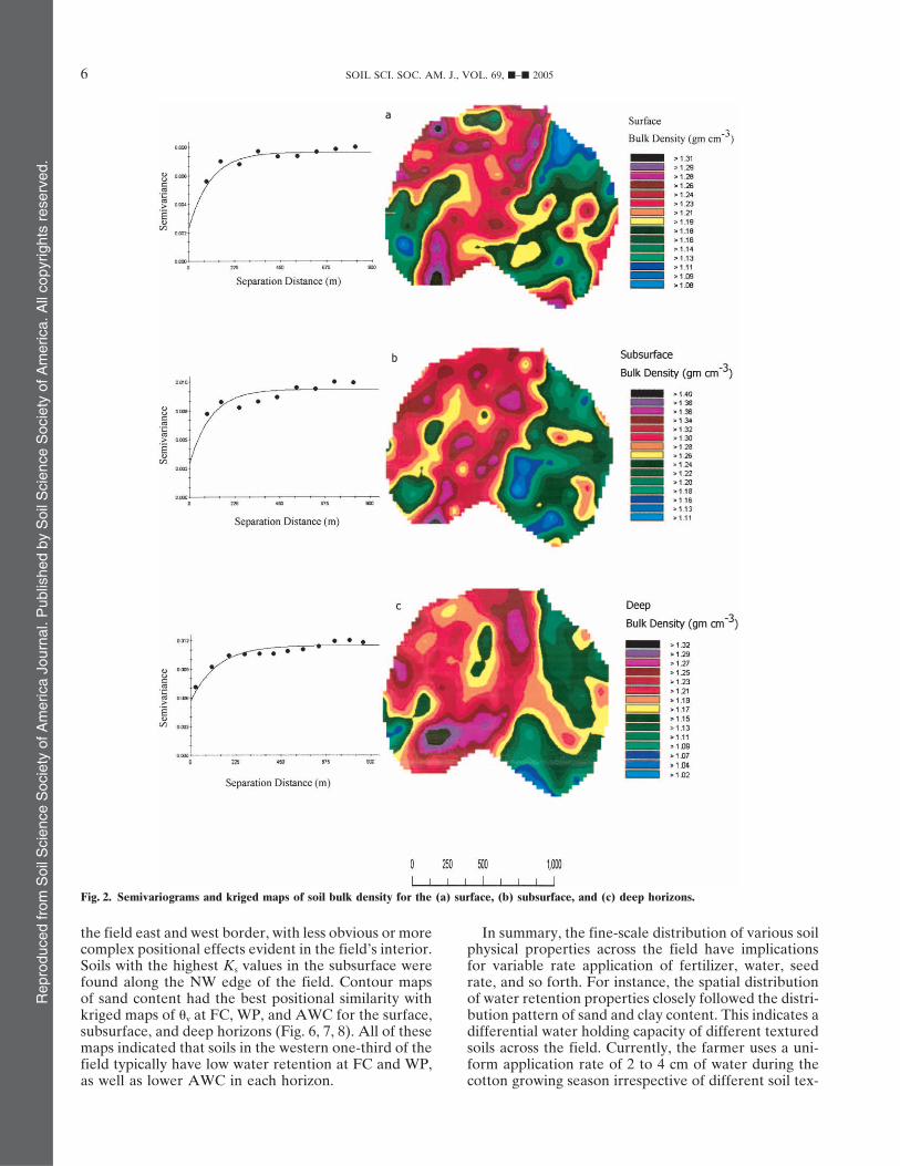
Spatial structure analysis indicated spatial variabilityacross field for soil texture, �b, water retention, and Ks.RESULTS AND DISCUSSIONWith regard to �b, the values for nugget, sill, % nugget,

Variation among Soil Horizons and range increased from the surface to the deep hori-zon. This increase indicated higher structured variance,Values for �b in the subsurface horizon were signifi-nugget effect/random variability, and range with increasecantly (P � 0.05) greater than in the surface and deepin depth, which may indicate a depositional event or ahorizons (Table 1). Increased �b and very low values forseries of depositional events. Compared with the presentKs mean (6.03 cm d�1) and range (0.03–63.47 cm d�1)study, Tsegaye and Hill (1998) observed lower structuralin subsurface horizons indicate downward movementvariability in surface �b, as judged from a higher nuggetof water is restricted by a compacted subsurface layer(0.003) and lower sill (0.004), that is, percentage nuggetobserved at about 31- to 62-cm depth. This may be dueattributed 75% of total variability with a range valueto compaction of fine sandy or fine silt layers by theof 22 m. The lower range reported by Tsegaye and Hillusage of heavy machinery on the farm and monocul-(1998) could be due to a much smaller sampling intervalture (cotton).of 1 m in a relatively small area (45 by 37 m) locatedThe Ks of all surface horizons was on average abouton a level landscape. The semivariogram functions fortwo times greater than for deep horizons, and four times

greater than all subsurface horizons. Increased Ks values Ks were exponential for the three horizons. In the sur-

Rep

rodu

ced

from

Soi

l Sci

ence

Soc

iety

of A

mer

ica

Jour

nal.

Pub

lishe

d by

Soi

l Sci

ence

Soc

iety

of A

mer

ica.

All

copy

right

s re

serv

ed.


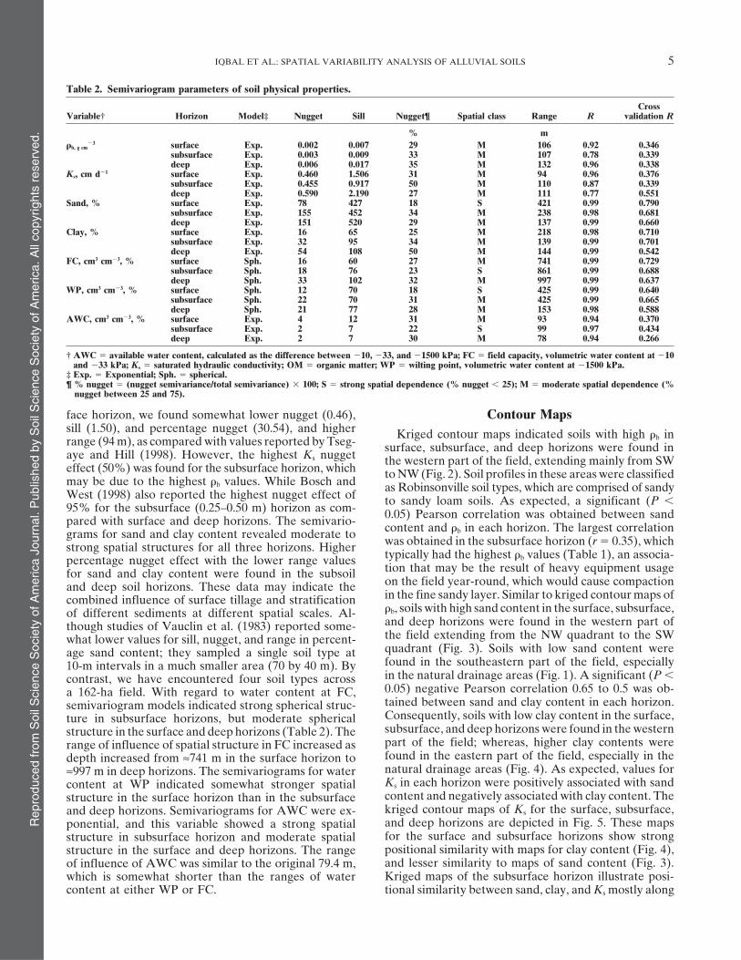
Table 2. Semivariogram parameters of soil physical properties.

CrossVariable† Horizon Model‡ Nugget Sill Nugget¶ Spatial class Range R validation R

% m�b, g cm

�3 surface Exp. 0.002 0.007 29 M 106 0.92 0.346subsurface Exp. 0.003 0.009 33 M 107 0.78 0.339deep Exp. 0.006 0.017 35 M 132 0.96 0.338

Ks, cm d�1 surface Exp. 0.460 1.506 31 M 94 0.96 0.376subsurface Exp. 0.455 0.917 50 M 110 0.87 0.339deep Exp. 0.590 2.190 27 M 111 0.77 0.551

Sand, % surface Exp. 78 427 18 S 421 0.99 0.790subsurface Exp. 155 452 34 M 238 0.98 0.681deep Exp. 151 520 29 M 137 0.99 0.660

Clay, % surface Exp. 16 65 25 M 218 0.98 0.710subsurface Exp. 32 95 34 M 139 0.99 0.701deep Exp. 54 108 50 M 144 0.99 0.542

FC, cm3 cm�3, % surface Sph. 16 60 27 M 741 0.99 0.729subsurface Sph. 18 76 23 S 861 0.99 0.688deep Sph. 33 102 32 M 997 0.99 0.637

WP, cm3 cm�3, % surface Sph. 12 70 18 S 425 0.99 0.640subsurface Sph. 22 70 31 M 425 0.99 0.665deep Sph. 21 77 28 M 153 0.98 0.588

AWC, cm3 cm�3, % surface Exp. 4 12 31 M 93 0.94 0.370subsurface Exp. 2 7 22 S 99 0.97 0.434deep Exp. 2 7 30 M 78 0.94 0.266

† AWC � available water content, calculated as the difference between �10, �33, and �1500 kPa; FC � field capacity, volumetric water content at �10and �33 kPa; Ks � saturated hydraulic conductivity; OM � organic matter; WP � wilting point, volumetric water content at �1500 kPa.

‡ Exp. � Exponential; Sph. � spherical.¶ % nugget � (nugget semivariance/total semivariance) � 100; S � strong spatial dependence (% nugget � 25); M � moderate spatial dependence (%

nugget between 25 and 75).

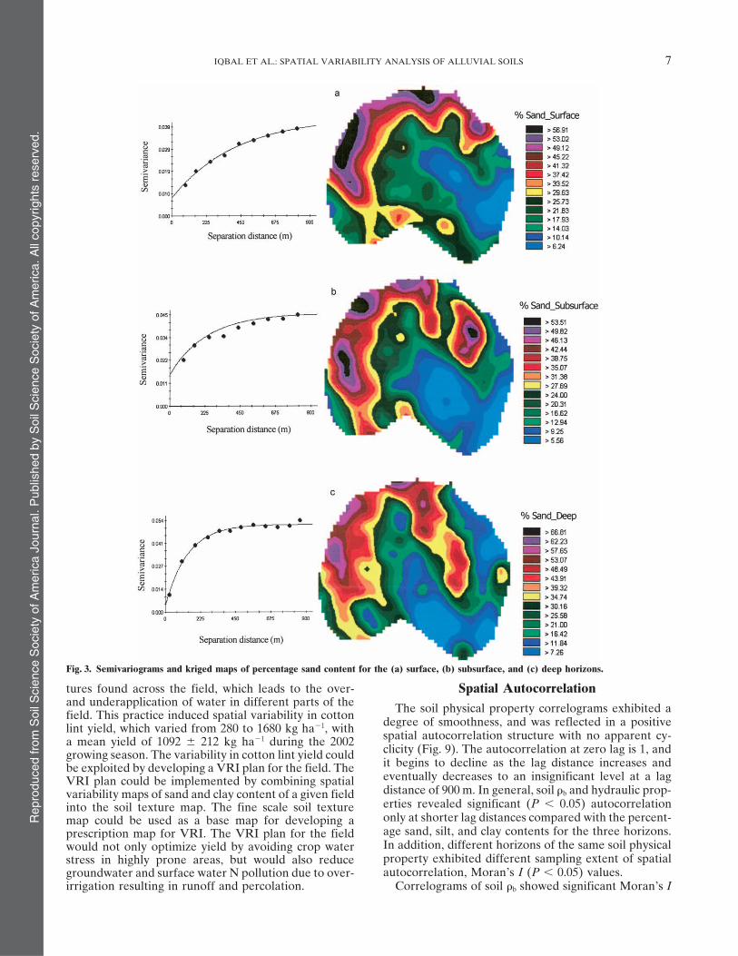
face horizon, we found somewhat lower nugget (0.46), Contour Mapssill (1.50), and percentage nugget (30.54), and higher Kriged contour maps indicated soils with high �b inrange (94 m), as compared with values reported by Tseg- surface, subsurface, and deep horizons were found inaye and Hill (1998). However, the highest Ks nugget the western part of the field, extending mainly from SWeffect (50%) was found for the subsurface horizon, which to NW (Fig. 2). Soil profiles in these areas were classifiedmay be due to the highest �b values. While Bosch and as Robinsonville soil types, which are comprised of sandyWest (1998) also reported the highest nugget effect of to sandy loam soils. As expected, a significant (P �95% for the subsurface (0.25–0.50 m) horizon as com- 0.05) Pearson correlation was obtained between sandpared with surface and deep horizons. The semivario- content and �b in each horizon. The largest correlationgrams for sand and clay content revealed moderate to was obtained in the subsurface horizon (r � 0.35), whichstrong spatial structures for all three horizons. Higher

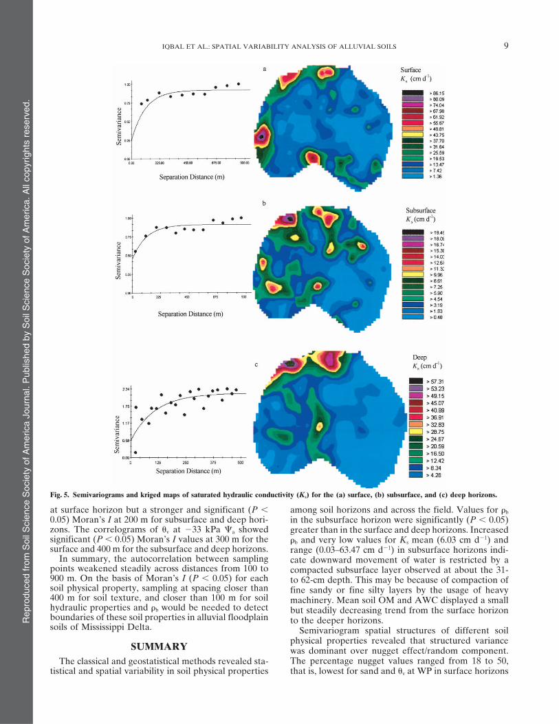
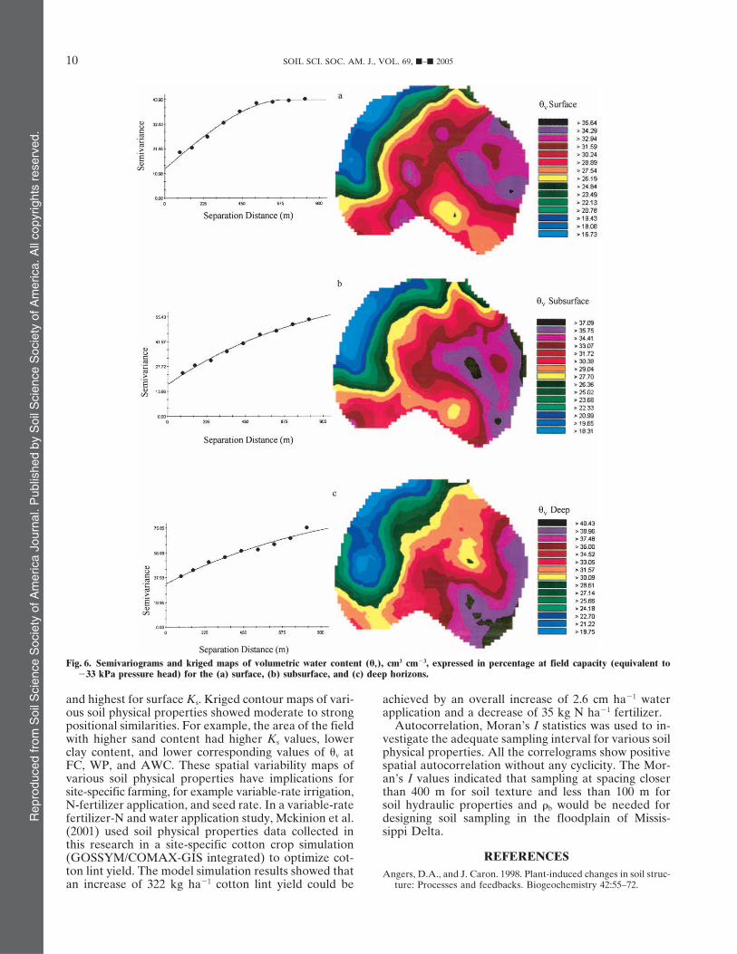
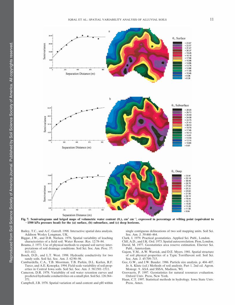
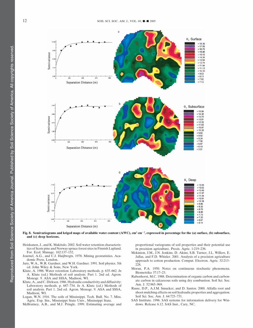
typically had the highest �b values (Table 1), an associa-percentage nugget effect with the lower range valuestion that may be the result of heavy equipment usagefor sand and clay content were found in the subsoilon the field year-round, which would cause compactionand deep soil horizons. These data may indicate thein the fine sandy layer. Similar to kriged contour maps ofcombined influence of surface tillage and stratification�b, soils with high sand content in the surface, subsurface,of different sediments at different spatial scales. Al-and deep horizons were found in the western part ofthough studies of Vauclin et al. (1983) reported some-the field extending from the NW quadrant to the SWwhat lower values for sill, nugget, and range in percent-quadrant (Fig. 3). Soils with low sand content wereage sand content; they sampled a single soil type atfound in the southeastern part of the field, especially10-m intervals in a much smaller area (70 by 40 m). Byin the natural drainage areas (Fig. 1). A significant (P �contrast, we have encountered four soil types across0.05) negative Pearson correlation 0.65 to 0.5 was ob-a 162-ha field. With regard to water content at FC,tained between sand and clay content in each horizon.semivariogram models indicated strong spherical struc-Consequently, soils with low clay content in the surface,ture in subsurface horizons, but moderate sphericalsubsurface, and deep horizons were found in the westernstructure in the surface and deep horizons (Table 2). Thepart of the field; whereas, higher clay contents wererange of influence of spatial structure in FC increased asfound in the eastern part of the field, especially in thedepth increased from ≈741 m in the surface horizon tonatural drainage areas (Fig. 4). As expected, values for≈997 m in deep horizons. The semivariograms for waterKs in each horizon were positively associated with sandcontent at WP indicated somewhat stronger spatialcontent and negatively associated with clay content. Thestructure in the surface horizon than in the subsurfacekriged contour maps of Ks for the surface, subsurface,and deep horizons. Semivariograms for AWC were ex-and deep horizons are depicted in Fig. 5. These mapsponential, and this variable showed a strong spatialfor the surface and subsurface horizons show strongstructure in subsurface horizon and moderate spatialpositional similarity with maps for clay content (Fig. 4),structure in the surface and deep horizons. The rangeand lesser similarity to maps of sand content (Fig. 3).of influence of AWC was similar to the original 79.4 m,Kriged maps of the subsurface horizon illustrate posi-which is somewhat shorter than the ranges of water

content at either WP or FC. tional similarity between sand, clay, and Ks mostly along

Rep

rodu

ced

from

Soi

l Sci

ence

Soc

iety

of A

mer

ica

Jour

nal.

Pub

lishe

d by

Soi

l Sci

ence

Soc

iety

of A

mer

ica.

All

copy

right

s re

serv

ed.


Fig. 2. Semivariograms and kriged maps of soil bulk density for the (a) surface, (b) subsurface, and (c) deep horizons.

the field east and west border, with less obvious or more In summary, the fine-scale distribution of various soilphysical properties across the field have implicationscomplex positional effects evident in the field’s interior.

Soils with the highest Ks values in the subsurface were for variable rate application of fertilizer, water, seedrate, and so forth. For instance, the spatial distributionfound along the NW edge of the field. Contour maps

of sand content had the best positional similarity with of water retention properties closely followed the distri-bution pattern of sand and clay content. This indicates akriged maps of �v at FC, WP, and AWC for the surface,

subsurface, and deep horizons (Fig. 6, 7, 8). All of these differential water holding capacity of different texturedsoils across the field. Currently, the farmer uses a uni-maps indicated that soils in the western one-third of the

field typically have low water retention at FC and WP, form application rate of 2 to 4 cm of water during thecotton growing season irrespective of different soil tex-as well as lower AWC in each horizon.

Rep

rodu

ced

from

Soi

l Sci

ence

Soc

iety

of A

mer

ica

Jour

nal.

Pub

lishe

d by

Soi

l Sci

ence

Soc

iety

of A

mer

ica.

All

copy

right

s re

serv

ed.


Fig. 3. Semivariograms and kriged maps of percentage sand content for the (a) surface, (b) subsurface, and (c) deep horizons.

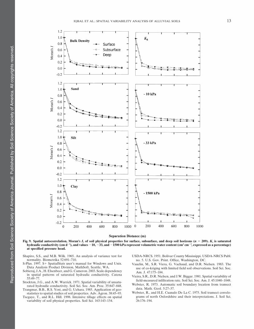
tures found across the field, which leads to the over- Spatial Autocorrelationand underapplication of water in different parts of the The soil physical property correlograms exhibited afield. This practice induced spatial variability in cotton degree of smoothness, and was reflected in a positivelint yield, which varied from 280 to 1680 kg ha�1, with

spatial autocorrelation structure with no apparent cy-a mean yield of 1092 � 212 kg ha�1 during the 2002clicity (Fig. 9). The autocorrelation at zero lag is 1, andgrowing season. The variability in cotton lint yield couldit begins to decline as the lag distance increases andbe exploited by developing a VRI plan for the field. Theeventually decreases to an insignificant level at a lagVRI plan could be implemented by combining spatialdistance of 900 m. In general, soil �b and hydraulic prop-variability maps of sand and clay content of a given fielderties revealed significant (P � 0.05) autocorrelationinto the soil texture map. The fine scale soil textureonly at shorter lag distances compared with the percent-map could be used as a base map for developing aage sand, silt, and clay contents for the three horizons.prescription map for VRI. The VRI plan for the fieldIn addition, different horizons of the same soil physicalwould not only optimize yield by avoiding crop waterproperty exhibited different sampling extent of spatialstress in highly prone areas, but would also reduceautocorrelation, Moran’s I (P � 0.05) values.groundwater and surface water N pollution due to over-

irrigation resulting in runoff and percolation. Correlograms of soil �b showed significant Moran’s I

Rep

rodu

ced

from

Soi

l Sci

ence

Soc

iety

of A

mer

ica

Jour

nal.

Pub

lishe

d by

Soi

l Sci

ence

Soc

iety

of A

mer

ica.

All

copy

right

s re

serv

ed.


Fig. 4. Semivariograms and kriged maps of percentage clay content for the (a) surface, (b) subsurface, and (c) deep horizons.

at lag distance of 100 m for surface and deep horizons stratification extents for the same soil physical propertyat different horizons. This suggests that the degree ofand 300 m for subsurface horizons. Sand and silt content

had a similar pattern of spatial autocorrelation extent cumulization and the extent of stratification during de-position of the alluvial materials is the most importantfor the three horizons: that is, each soil property showed

a significant Moran’s I at 600 m for the surface and factor in explaining the significant extent of spatial auto-correlation, Moran’s I differences at surface, subsurface,400 m for the subsurface and deep horizons. However,

the clay content correlogram had a significant Moran’s and deep horizons. Those differences and anthropo-genic activities, like subsoiling, affected the spatial auto-I at 400 m for surface and subsurface horizons and

300 m for deep horizons. Soils in the Mississippi Delta, correlation of soil hydraulic properties in the surfaceand subsurface horizons. The correlograms of Ks andespecially along the Mississippi River, are minimally

developed Entisols showing little evidence of pedo- � at �1500 kPa had a significant (P � 0.05) Moran’sI at 100 m for three horizons; however, Ks showedgensis, and diagnostic surface and subsurface horizons

are typically absent; therefore, differences in the particle stronger autocorrelation for deep horizons when com-pared with the surface and subsurface horizons. Thesize and its spatial autocorrelation extent are not likely

related to pedogenic processes, such as eluvation and correlograms of �v at �10 kPa �a showed a weaklysignificant (P � 0.1) autocorrelation, Moran’s I at 100 milluviation. These alluvial floodplain soils have different

Rep

rodu

ced

from

Soi

l Sci

ence

Soc

iety

of A

mer

ica

Jour

nal.

Pub

lishe

d by

Soi

l Sci

ence

Soc

iety

of A

mer

ica.

All

copy

right

s re

serv

ed.


Fig. 5. Semivariograms and kriged maps of saturated hydraulic conductivity (Ks) for the (a) surface, (b) subsurface, and (c) deep horizons.

at surface horizon but a stronger and significant (P � among soil horizons and across the field. Values for �b

0.05) Moran’s I at 200 m for subsurface and deep hori- in the subsurface horizon were significantly (P � 0.05)zons. The correlograms of �v at �33 kPa �a showed greater than in the surface and deep horizons. Increasedsignificant (P � 0.05) Moran’s I values at 300 m for the �b and very low values for Ks mean (6.03 cm d�1) andsurface and 400 m for the subsurface and deep horizons. range (0.03–63.47 cm d�1) in subsurface horizons indi-

In summary, the autocorrelation between sampling cate downward movement of water is restricted by apoints weakened steadily across distances from 100 to compacted subsurface layer observed at about the 31-900 m. On the basis of Moran’s I (P � 0.05) for each to 62-cm depth. This may be because of compaction ofsoil physical property, sampling at spacing closer than fine sandy or fine silty layers by the usage of heavy400 m for soil texture, and closer than 100 m for soil machinery. Mean soil OM and AWC displayed a smallhydraulic properties and �b would be needed to detect but steadily decreasing trend from the surface horizonboundaries of these soil properties in alluvial floodplain to the deeper horizons.soils of Mississippi Delta. Semivariogram spatial structures of different soil

physical properties revealed that structured varianceSUMMARY was dominant over nugget effect/random component.

The percentage nugget values ranged from 18 to 50,The classical and geostatistical methods revealed sta-tistical and spatial variability in soil physical properties that is, lowest for sand and �v at WP in surface horizons

Rep

rodu

ced

from

Soi

l Sci

ence

Soc

iety

of A

mer

ica

Jour

nal.

Pub

lishe

d by

Soi

l Sci

ence

Soc

iety

of A

mer

ica.

All

copy

right

s re

serv

ed.


Fig. 6. Semivariograms and kriged maps of volumetric water content (�v), cm3 cm�3, expressed in percentage at field capacity (equivalent to�33 kPa pressure head) for the (a) surface, (b) subsurface, and (c) deep horizons.

and highest for surface Ks. Kriged contour maps of vari- achieved by an overall increase of 2.6 cm ha�1 waterapplication and a decrease of 35 kg N ha�1 fertilizer.ous soil physical properties showed moderate to strong

positional similarities. For example, the area of the field Autocorrelation, Moran’s I statistics was used to in-vestigate the adequate sampling interval for various soilwith higher sand content had higher Ks values, lower

clay content, and lower corresponding values of �v at physical properties. All the correlograms show positivespatial autocorrelation without any cyclicity. The Mor-FC, WP, and AWC. These spatial variability maps of

various soil physical properties have implications for an’s I values indicated that sampling at spacing closerthan 400 m for soil texture and less than 100 m forsite-specific farming, for example variable-rate irrigation,

N-fertilizer application, and seed rate. In a variable-rate soil hydraulic properties and �b would be needed fordesigning soil sampling in the floodplain of Missis-fertilizer-N and water application study, Mckinion et al.

(2001) used soil physical properties data collected in sippi Delta.this research in a site-specific cotton crop simulation

REFERENCES(GOSSYM/COMAX-GIS integrated) to optimize cot-ton lint yield. The model simulation results showed that Angers, D.A., and J. Caron. 1998. Plant-induced changes in soil struc-

ture: Processes and feedbacks. Biogeochemistry 42:55–72.an increase of 322 kg ha�1 cotton lint yield could be

Rep

rodu

ced

from

Soi

l Sci

ence

Soc

iety

of A

mer

ica

Jour

nal.

Pub

lishe

d by

Soi

l Sci

ence

Soc

iety

of A

mer

ica.

All

copy

right

s re

serv

ed.


Fig. 7. Semivariograms and kriged maps of volumetric water content (�v), cm3 cm�3, expressed in percentage at wilting point (equivalent to�1500 kPa pressure head) for the (a) surface, (b) subsurface, and (c) deep horizons.

Bailey, T.C., and A.C. Gatrell. 1998. Interactive spatial data analysis. single contiguous delineations of two soil mapping units. Soil Sci.Soc. Am. J. 39:460–464.Addison Wesley Longman, UK.

Biggar, J.W., and D.R. Nielsen. 1976. Spatial variability of leaching Clark, I. 1979. Practical geostatistics. Applied Sci. Publ., London.Cliff, A.D., and J.K. Ord. 1973. Spatial autocorrelation. Pion, London.characteristics of a field soil. Water Resour. Res. 12:78–84.

Bouma, J. 1973. Use of physical methods to expand soil survey inter- David, M. 1977. Geostatistics area reserve estimation. Elsevier Sci.Publ., Amsterdam.pretations of soil drainage conditions. Soil Sci. Soc. Am. Proc. 37:

413–412. Gajem, Y.M., A.W. Warrick, and D.E. Myers. 1981. Spatial structureof soil physical properties of a Typic Torrifluvent soil. Soil Sci.Bosch, D.D., and L.T. West. 1998. Hydraulic conductivity for two

sandy soils. Soil Sci. Soc. Am. J. 62:90–98. Soc. Am. J. 45:709–715.Gee, G.W., and J.W. Bauder. 1986. Particle size analysis. p. 404–407.Cambardella, C.A., T.B. Moorman, T.B. Parkin, D.L. Karlen, R.F.

Turco, and A.E. Konopka. 1994. Field scale variability of soil prop- In A. Klute (ed.) Methods of soil analysis. Part 1. 2nd ed. Agron.Monogr. 9. ASA and SSSA, Madison, WI.erties in Central Iowa soils. Soil Sci. Soc. Am. J. 58:1501–1511.

Cameron, D.R. 1978. Variability of soil water retention curves and Goovaerts, P. 1997. Geostatistics for natural resources evaluation.Oxford Univ. Press, New York.predicted hydraulic conductivities on a small plot. Soil Sci. 126:364–

371. Haan, C.T. 1997. Statistical methods in hydrology. Iowa State Univ.Press, Ames.Campbell, J.B. 1978. Spatial variation of sand content and pH within

Rep

rodu

ced

from

Soi

l Sci

ence

Soc

iety

of A

mer

ica

Jour

nal.

Pub

lishe

d by

Soi

l Sci

ence

Soc

iety

of A

mer

ica.

All

copy

right

s re

serv

ed.


Fig. 8. Semivariograms and kriged maps of available water content (AWC), cm3 cm�3, expressed in percentage for the (a) surface, (b) subsurface,and (c) deep horizons.

Heiskanen, J., and K. Makitalo. 2002. Soil water retention characteris- proportional variograms of soil properties and their potential usetics of Scots pine and Norway spruce forest sites in Finnish Lapland. in precision agriculture. Precis. Agric. 1:219–236.For. Ecol. Manage. 162:137–152. Mckinion, J.M., J.N. Jenkins, D. Akins, S.B. Turner, J.L. Willers, E.

Journel, A.G., and C.J. Huijbregts. 1978. Mining geostatistics. Aca- Jallas, and F.D. Whisler. 2001. Analysis of a precision agriculturedemic Press, London. approach to cotton production. Comput. Electron. Agric. 32:213–

Jury, W.A., W.R. Gardner, and W.H. Gardner. 1991. Soil physics. 5th 228.ed. John Wiley & Sons, New York. Moran, P.A. 1950. Notes on continuous stochastic phenomena.

Klute, A. 1986. Water retention: Laboratory methods. p. 635–662. In Biometrika 37:17–23.A. Klute (ed.) Methods of soil analysis. Part 1. 2nd ed. Agron.

Rabenhorst, M.C. 1988. Determination of organic carbon and carbon-Monogr. 9. ASA and SSSA, Madison, WI.ate carbon in calcareous soils using dry combustion. Soil Sci. Soc.Klute, A., and C. Dirksen. 1986. Hydraulic conductivity and diffusivity:Am. J. 52:965–969.Laboratory methods. p. 687–734. In A. Klute (ed.) Methods of

Rasse, D.P., A.J.M. Smucker, and D. Santos. 2000. Alfalfa root andsoil analysis. Part 1. 2nd ed. Agron. Monogr. 9. ASA and SSSA,shoot mulching effects on soil hydraulic properties and aggregation.Madison, WI.Soil Sci. Soc. Am. J. 64:725–731.Logan, W.N. 1916. The soils of Mississippi. Tech. Bull. No. 7. Miss.

SAS Institute. 1996. SAS systems for information delivery for Win-Agric. Exp. Stn., Mississippi State Univ., Mississippi State.McBratney, A.B., and M.J. Pringle. 1999. Estimating average and dows. Release 6.12. SAS Inst., Cary, NC.

Rep

rodu

ced

from

Soi

l Sci

ence

Soc

iety

of A

mer

ica

Jour

nal.

Pub

lishe

d by

Soi

l Sci

ence

Soc

iety

of A

mer

ica.

All

copy

right

s re

serv

ed.


Fig. 9. Spatial autocorrelation, Moran’s I, of soil physical properties for surface, subsurface, and deep soil horizons (n � 209). Ks is saturatedhydraulic conductivity (cm d�1), and values �10, �33, and �1500 kPa represent volumetric water content (cm3 cm�3, expressed as a percentage)at specified pressure head.

Shapiro, S.S., and M.B. Wilk. 1965. An analysis of variance test for USDA-NRCS. 1951. Bolivar County Mississippi. USDA-NRCS Publ.normality. Biometrika 52:691–710. no. 5. U.S. Gov. Print. Office, Washington, DC.

S-Plus. 1997. S� SpatialStats user’s manual for Windows and Unix. Vauclin, M., S.R. Viera, G. Vachaud, and D.R. Nielsen. 1983. TheData Analysis Product Division, MathSoft, Seattle, WA. use of co-kriging with limited field soil observations. Soil Sci. Soc.

Sobieraj, J.A., H. Elsenbeer, and G. Cameron. 2003. Scale dependency Am. J. 47:175–184.in spatial patterns of saturated hydraulic conductivity. Catena Vieira, S.R., D.R. Nielsen, and J.W. Biggar. 1981. Spatial variability of55:49–77.

field-measured infiltration rate. Soil Sci. Soc. Am. J. 45:1040–1048.Stockton, J.G., and A.W. Warrick. 1971. Spatial variability of unsatu-Webster, R. 1973. Automatic soil boundary location from transectrated hydraulic conductivity. Soil Sci. Soc. Am. Proc. 35:847–848.

data. Math. Geol. 5:27–37.Trangmar, B.B., R.S. Yost, and G. Uehara. 1985. Application of geo-Webster, R., and H.E. Cuanalo De La C. 1975. Soil transect correlo-statistics to spatial studies of soil properties. Adv. Agron. 38:45–93.

grams of north Oxfordshire and their interpretations. J. Soil Sci.Tsegaye, T., and R.L. Hill. 1998. Intensive tillage effects on spatialvariability of soil physical properties. Soil Sci. 163:143–154. 26:176–194.

Rep

rodu

ced

from

Soi

l Sci

ence

Soc

iety

of A

mer

ica

Jour

nal.

Pub

lishe

d by

Soi

l Sci

ence

Soc

iety

of A

mer

ica.

All

copy

right

s re

serv

ed.


soil spatial sssaj

Documents