Experiment No. 1: Soil Moisture Content

Aim

Determination of moisture content (water content) of soil.

ApparatusDrying oven, Non-corrodible metal cans with lids, Balance (0.001 g accuracy for fine-grained soils), Spatula, Gloves.

Procedure

1. Record the number of can and lid. Clean, dry, and record their weight.

2. Using a spatula, place about 15-30 g of moist soil in the can. Secure the lid, weigh and record.

3. Maintain the temperature of the oven at 110 ± 5°C. Open the lid, and place the can in the oven. Leave it overnight.

4. After drying, remove the can carefully from the oven using gloves or tongs. Allow it to cool to room temperature.

5. Weigh the dry soil in the can along with lid.

6. For each soil, perform at least 3 sets of the test.

Observations and Calculations

Tabulate observations and results of the tests as shown.

Test No. 1 2 3 4Can No. Mass of can with lid,

Mass of can with lid + wet soil,

Mass of can with lid + dry soil,

Mass of water,

Mass of dry soil,

Moisture content,

ResultAverage moisture content, w (%) =

Experiment No. 2: Soil Specific Gravity

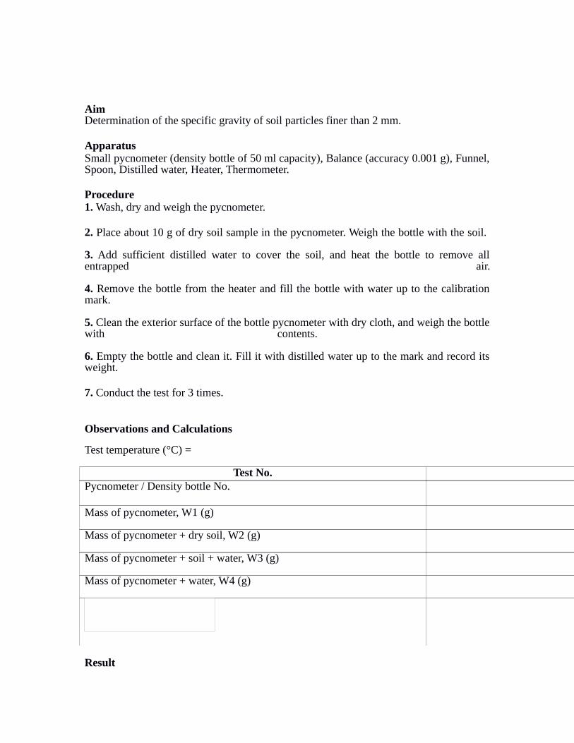
AimDetermination of the specific gravity of soil particles finer than 2 mm.

ApparatusSmall pycnometer (density bottle of 50 ml capacity), Balance (accuracy 0.001 g), Funnel, Spoon, Distilled water, Heater, Thermometer.

Procedure1. Wash, dry and weigh the pycnometer.

2. Place about 10 g of dry soil sample in the pycnometer. Weigh the bottle with the soil.

3. Add sufficient distilled water to cover the soil, and heat the bottle to remove all entrapped air.

4. Remove the bottle from the heater and fill the bottle with water up to the calibration mark.

5. Clean the exterior surface of the bottle pycnometer with dry cloth, and weigh the bottle with contents.

6. Empty the bottle and clean it. Fill it with distilled water up to the mark and record its weight.

7. Conduct the test for 3 times.

Observations and Calculations

Test temperature (°C) =

Test No.Pycnometer / Density bottle No.

Mass of pycnometer, W1 (g)

Mass of pycnometer + dry soil, W2 (g)

Mass of pycnometer + soil + water, W3 (g)

Mass of pycnometer + water, W4 (g)

Specific gravity of soil,

Result

Average specific gravity of soil grains =

Experiment No.3: Grain size analysis – Mechanical Method

AimDetermination of quantitative size distribution of particles of soil down to fine-grained fraction.

ApparatusSet of sieves (4.75 mm, 2.8 mm, 2 mm, 1 mm, 600 micron, 425 micron, 300 micron, 150 micron, 75 micron), Balance (0.1 g accuracy), Drying oven, Rubber pestle, Cleaning brush, Mechanical shaker.

Procedure

1. Take a suitable quantity of oven-dried soil. The mass of soil sample required for each test depends on the maximum size of material.

2. Clean the sieves to be used, and record the weight of each sieve and the bottom pan.

3. Arrange the sieves to have the largest mesh size at the top of the stack. Pour carefully the soil sample into the top sieve and place the lid over it.

4. Place the sieve stack on the mechanical shaker, screw down the lid, and vibrate the soil sample for 10 minutes.

5. Remove the stack and re-weigh each sieve and the bottom pan with the soil sample fraction retained on it.

Observations and Calculations

Initial mass of soil sample taken for analysis (kg) =

Sieve size

(mm)

Mass of sieve

(g)

Mass of sieve + soil

(g)

Soil retained

(g)

Percent retained

(%)

Cumulative

percent retained

(%)

Percent finer

(%)

4.75 mm 2.8 mm 2 mm 1 mm

600 micron 425 micron 300 micron 150 micron 75 micron

Pan

1. Obtain the mass of soil retained on each sieve. The sum of the retained masses should be approximately equal to the initial mass of the soil sample.

2. Calculate the percent retained on each sieve by dividing the mass retained on the sieve with the total initial mass of the soil.

3. Calculate the cumulative percent retained by adding percent retained on each sieve as a cumulative procedure.

4. Calculate the percent finer by subtracting the cumulative percent retained from 100 percent.

5. Make a grain size distribution curve by plotting sieve size on log scale and percent finer on ordinary scale.

6. Read off the sizes corresponding to 60%, 30% and 10% finer. Calculate the uniformity coefficient (Cu) and the curvature coefficient (Cc) for the soil.

Result

Coefficient of uniformity (Cu) of the soil =

Coefficient of curvature (Cc) of the soil =

Experiment No. 4: Grain size analysis – Hydrometer analysis

AimDetermination of the quantitative size distribution of particles of soil fraction finer than 75 micron.

ApparatusHydrometer (calibrated at 27°C, range of 0.995 to 1.030 g/cc), Two 1000 ml graduated glass cylinders, Dispersing agent solution containing sodium hexametaphosphate, Evaporating dish, Thermometer, Stop-watch, Mechanical stirrer.

Procedure

1. Take 50 g of dry soil in an evaporating dish, add 100 ml of dispersing agent, and prepare a suspension.

2. Transfer the suspension into the cup of a mechanical stirrer, add more distilled water, and operate the stirrer for three minutes.

3. Wash the soil slurry into a cylinder, and add distilled water to bring up the level to the 1000 ml mark.

4. Cover the open end of the cylinder with a stopper and hold it securely with the palm of the hand. Then turn the cylinder upside down and back upright repeatedly for one minute.

5. Place the cylinder down and remove the stopper. Insert a hydrometer and start a stop-watch simultaneously. To minimize bobbing of the hydrometer, it should be released close to the reading depth. This requires some amount of rehearsal and practice.

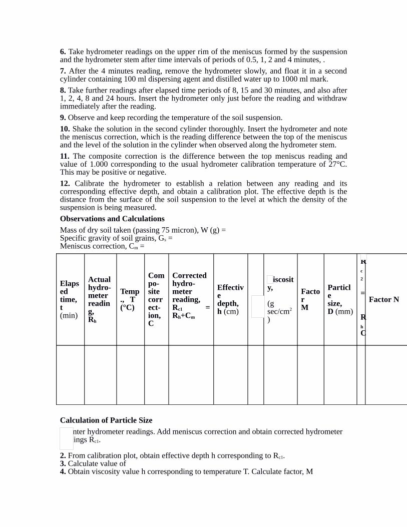
6. Take hydrometer readings on the upper rim of the meniscus formed by the suspension and the hydrometer stem after time intervals of periods of 0.5, 1, 2 and 4 minutes, .

7. After the 4 minutes reading, remove the hydrometer slowly, and float it in a second cylinder containing 100 ml dispersing agent and distilled water up to 1000 ml mark.

8. Take further readings after elapsed time periods of 8, 15 and 30 minutes, and also after 1, 2, 4, 8 and 24 hours. Insert the hydrometer only just before the reading and withdraw immediately after the reading.

9. Observe and keep recording the temperature of the soil suspension.

10. Shake the solution in the second cylinder thoroughly. Insert the hydrometer and note the meniscus correction, which is the reading difference between the top of the meniscus and the level of the solution in the cylinder when observed along the hydrometer stem.

11. The composite correction is the difference between the top meniscus reading and value of 1.000 corresponding to the usual hydrometer calibration temperature of 27°C. This may be positive or negative.

12. Calibrate the hydrometer to establish a relation between any reading and its corresponding effective depth, and obtain a calibration plot. The effective depth is the distance from the surface of the soil suspension to the level at which the density of the suspension is being measured.

Observations and Calculations

Mass of dry soil taken (passing 75 micron), W (g) =Specific gravity of soil grains, Gs =Meniscus correction, Cm =

Elapsed time, t(min)

Actualhydro-meterreading, Rh

Temp., T (°C)

Compo-sitecorrect-ion, C

Corrected hydro-meterreading,Rc1 = Rh+Cm

Effective depth,h (cm)

Viscosity,

(g sec/cm2

)

FactorM

Particlesize, D (mm)

Rc

2

=

Rh

C

Factor N

Calculation of Particle Size

1. Enter hydrometer readings. Add meniscus correction and obtain corrected hydrometer readings Rc1.

2. From calibration plot, obtain effective depth h corresponding to Rc1. 3. Calculate value of 4. Obtain viscosity value h corresponding to temperature T. Calculate factor, M

5. Calculate particle size D by multiplying M and

Calculation of Percentage Finer

1. Add the composite correction C to the hydrometer reading to get another corrected hydrometer reading Rc2.2. Calculate factor, N

3. Calculate percentage finer F by multiplying Rc2 and N. 4. Calculate percentage finer with respect to total mass of soil taken for sieve analysis and hydrometer analysis.

Total percent finer = F x fine-grained percent in the total soil mass.

Present results by plotting particle size vs. percent finer on a semi-logarithmic sheet.

Experiment No. 5: Atterberg limits determination – Liquid Limit, Plastic Limit, Shrinkage Limit

AimDetermination of the liquid and plastic limits of a soil.

ApparatusLiquid limit device and grooving tools, Metal rod of 3 mm diameter, Apparatus for moisture content determination, Porcelain evaporating dish, Spatula, Wash bottle filled with distilled water, Measuring cylinder, Glass plate.

Procedure for Liquid Limit

1. Take about 150 gm of dry soil passing 425 micron sieve, and mix it with distilled water in a porcelain dish to form a uniform paste.

2. Place a portion of the paste in the cup of liquid limit device with a spatula, press the soil down to remove air pockets, spread it to a maximum depth of 10 mm, and form an approximately horizontal surface.

3. By holding a grooving tool perpendicular to the cup, carefully cut through the sample from back to front, and form a clean straight groove in the centre by dividing into two halves.

4. Turn the crank handle of the device at a steady rate of two revolutions per second. Continue turning until the two halves of the groove is closed along a distance of 13 mm. Record the number of blows to reach this condition.

5. Take about 15 gm of the soil from the joined portion of the groove to a moisture can for determining water content.

6. Transfer the remaining soil from the cup into the porcelain dish. Clean and dry the cup and the grooving tool.

7. Repeat steps 2 to 6, and obtain at least four sets of readings evenly spaced out in the range of 10 to 40 blows.

Procedure for Plastic Limit

1. Use the remaining soil from the porcelain dish.

2. Take about 10 gm of the soil mass in the hand, form a ball, and roll it between the palm or the fingers and the glass plate using complete motion of the hand forward and reverse.

3. Apply only sufficient pressure to make a soil thread, and continue rolling until a thread of 3 mm diameter is formed. Comparison can be made with the metal rod.

4. If the diameter becomes less than 3 mm without cracking, turn the soil into a ball again, and re-roll. Repeat this remoulding and rolling process until the thread starts just crumbling at a diameter of 3 mm.

5. Gather the pieces of crumbled thread and place them in a moisture can for determining water content.

6. Repeat steps 2 to 5 at least two more times with fresh samples of 10 gm each.

Observations and Calculations

Determination of Liquid Limit

Test No. 1 2 3 4 5No. of blows Can No. Mass of can (g) Mass of can + wet.soil, (g) Mass of can + dry soil, (g) Mass of water (g) Mass of dry soil (g) Water content (%)

Calculate the water contents, and plot the number of blows (on log scale) versus the water content (on ordinary scale). Draw the best-fit straight line through the points.

Liquid Limit = Water content corresponding to 25 blows

Determination of Plastic Limit

Test No. 1 2 3 4 5 Can No. Mass of can (g) Mass of can + wet soil, (g) Mass of can + dry soil, (g) Mass of water (g) Mass of dry soil (g) Water content (%)

Plastic Limit = Average of the computed water contents

Experiment No. 6: In-situ density of soils – Sand jar cone method

AimDetermination of the in-situ density of soils by core cutter method or sand replacement method.

Core Cutter MethodApparatus Cylindrical core cutter, Dolley, Rammer, Balance (1 g accuracy), Spade, Straight edge knife, Sample extruder, Apparatus for moisture content determination.

Procedure

1. Measure the internal dimensions of the core cutter and weigh it.

2. Clean and level the site surface where the field density is to be determined.

3. Place the dolley on the cutter and press both into the soil using the rammer until only about 15 mm of the dolley protrudes above the surrounding soil surface.

4. Remove the soil around the cutter with the spade, lift up the cutter, and trim carefully the top and bottom surfaces of the soil sample.

5. Clean the outside surface of the cutter and weigh it with the soil.

6. Remove the soil core from the cutter and take three representative samples in moisture cans for water content determination.

Sand Replacement MethodFor hard and gravelly soils, the core-cutter method is not suitable. In its place, sand replacement method can be used, and it involves making a hole in the ground, weighing the excavated soil and determining the volume of the hole.

ApparatusSand pouring cylinder, Calibrating cylinder, Clean and dry sand, Metal tray with a central circular hole, Balance (1 g accuracy), Glass plate, Trowel, Scraper tool, Apparatus for moisture content determination.

Procedure

1. An inverted cone forms the base of the sand pouring cylinder, and a shutter at the cone tip controls the release of sand through a uniform free fall.

2. First determine the bulk density of the sand to be used in the field. For this, measure the internal dimensions of the calibrating cylinder so as to obtain its volume. Fill the pouring cylinder with sand and weigh. Place it concentrically on top of the calibrating cylinder, and allow sand to run out and fill both the calibrating cylinder and the inverted conical portion.

3. To obtain only the mass of sand filling up the conical portion, lift the pouring cylinder and then weigh with remaining sand. Place it on a glass plate, and allow sand to run out. Weigh again the pouring cylinder with left over sand.

4. Calculate the mass of sand that fills up the calibrating cylinder, and from its known volume, work out the bulk density of the sand for the allowed free fall.

5. Clean and level the site surface, and place the square tray with a central hole. Excavate a hole of diameter equal to that of the tray hole and depth equal to about 15 cm. Collect the excavated soil in the tray, weigh and then take representative samples for water content determination.

6. Fill the pouring cylinder with the same sand, place it concentrically over the hole, open the shutter and allow sand to fill up the hole.

7. When there is no further movement of sand, close the shutter, remove the cylinder and weigh it with the remaining sand.

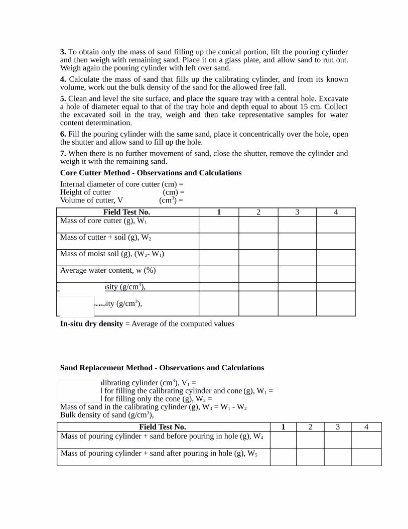
Core Cutter Method - Observations and Calculations

Internal diameter of core cutter (cm) =Height of cutter (cm) =Volume of cutter, V (cm3) =

Field Test No. 1 2 3 4Mass of core cutter (g), W1

Mass of cutter + soil (g), W2

Mass of moist soil (g), (W2- W1)

Average water content, w (%)

Field bulk density (g/cm3),

Field dry density (g/cm3),

In-situ dry density = Average of the computed values

Sand Replacement Method - Observations and Calculations

Volume of calibrating cylinder (cm3), V1 =Mass of sand for filling the calibrating cylinder and cone (g), W1 = Mass of sand for filling only the cone (g), W2 = Mass of sand in the calibrating cylinder (g), W3 = W1 - W2

Bulk density of sand (g/cm3),

Field Test No. 1 2 3 4Mass of pouring cylinder + sand before pouring in hole (g), W4

Mass of pouring cylinder + sand after pouring in hole (g), W5

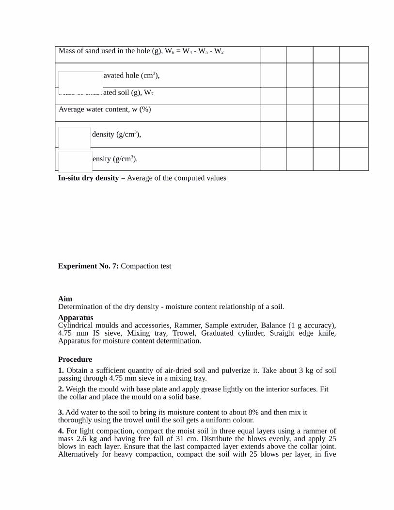
Mass of sand used in the hole (g), W6 = W4 - W5 - W2

Volume of excavated hole (cm3),

Mass of excavated soil (g), W7

Average water content, w (%)

Field bulk density (g/cm3),

Field dry density (g/cm3),

In-situ dry density = Average of the computed values

Experiment No. 7: Compaction test

AimDetermination of the dry density - moisture content relationship of a soil.

ApparatusCylindrical moulds and accessories, Rammer, Sample extruder, Balance (1 g accuracy), 4.75 mm IS sieve, Mixing tray, Trowel, Graduated cylinder, Straight edge knife, Apparatus for moisture content determination.

Procedure

1. Obtain a sufficient quantity of air-dried soil and pulverize it. Take about 3 kg of soil passing through 4.75 mm sieve in a mixing tray.

2. Weigh the mould with base plate and apply grease lightly on the interior surfaces. Fit the collar and place the mould on a solid base.

3. Add water to the soil to bring its moisture content to about 8% and then mix it thoroughly using the trowel until the soil gets a uniform colour.

4. For light compaction, compact the moist soil in three equal layers using a rammer of mass 2.6 kg and having free fall of 31 cm. Distribute the blows evenly, and apply 25 blows in each layer. Ensure that the last compacted layer extends above the collar joint. Alternatively for heavy compaction, compact the soil with 25 blows per layer, in five

equal layers with a rammer of mass 4.9 kg and 45 cm free fall.

5. Rotate the collar so as to remove it, trim off the compacted soil flush with the top of the mould, and weigh the mould with soil and base plate.

6. Extrude the soil from the mould and collect soil samples from the top, middle and bottom parts for water content determination. Place the soil back in the tray, add 2% more water based on the original soil mass, and re-mix as in step 3. Repeat steps 4 and 5 until a peak value of compacted soil mass is reached followed by a few samples of lesser compacted soil masses.

Observations and Calculations

Diameter of mould, d (cm) = Wt. of rammer (kg) =Height of mould, h (cm) = No. of layers =Volume of mould, V (cm3) = No. of blows/layer =Mass of mould, W (g) =

Test No. 1 2 3 4 5 6Mass of mould + compacted soil (g)

Mass of compacted soil, Wt (g)

Bulk density,

Average water content, w (%)

Dry density, (g/cc )

Dry density at 100% saturation (g/cc)

1. Calculate the bulk density of each compacted soil specimen.

2. Calculate the average moisture content of the compacted specimen and then its dry density.

3. Plot the dry densities obtained as ordinates against the corresponding moisture contents as abscissa, draw a smooth compaction curve passing through them, and obtain the values of maximum dry density (MDD) and optimum moisture content (OMC). 4. On the same graph, plot a curve corresponding to 100% saturation.

where, S = degree of saturation, Gs = specific gravity of solids, and gw = unit weight of water.

Results MDD (g/cc) =OMC (%) =

Experiment No. 8: Coefficient of permeability – Falling head method

AimDetermination of the coefficient of permeability of a soil using constant head apparatus or variable head apparatus.

ApparatusPermeameter mould and accessories, Circular filter papers, Compaction device, Constant head reservoir, Graduated glass standpipes along with support frame and clamps, Measuring flask, Stop-watch.

Procedure for Constant Head Test

1. Take 2.5 kg of dry soil and prepare it to obtain desired water content.

2. Apply little grease on to the interior sides of the permeameter mould.

3. Keep a solid metal plate in the groove of the compaction base plate. Assemble the base plate, mould and collar. Compact the soil into the mould.

4. Remove the collar and base plate, and replace the solid metal plate with a porous stone covered with filter paper.

5. Trim off excess soil from the top of the mould and place another porous stone with filter paper on it. Attach the top cap of the permeameter.

6. Connect a constant head reservoir to the bottom outlet of the mould. Open the air vent of the top cap, and allow water to flow in and upwards till the soil gets saturated.

7. Disconnect the reservoir from the bottom outlet and connect it to the top inlet. Close the air vent and allow water to establish a steady flow.

8. Collect the water in a measuring flask for a convenient time interval. For similar time intervals, measure the flow quantity for at least three times.

9. After the test, measure the temperature of the water.

Procedure for Variable Head Test

1. Follow the same steps 1 to 6 as for the constant head test.

2. Disconnect the reservoir from the bottom outlet and connect a selected standpipe to the top inlet.

3. Fill the standpipe with water, close the air vent and allow water to flow.

4. Open the bottom outlet and record the time interval required for the water surface in the standpipe to fall between two levels as measured from the centre of the outlet.

5. Measure time intervals for similar drops in head at least three times after re-filling the standpipe.

6. At the end of the test, measure the temperature of the water.

Observations and Calculations

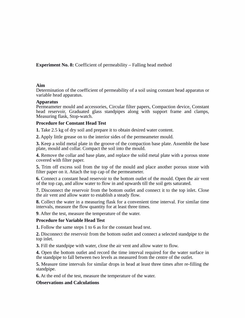
Constant Head FlowDiameter of sample, D (cm) = Length of sample, L (cm) =Area of sample, A (cm2) = Volume of sample, V (cm3) =Initial mass of sample, W (g) =initial water content, w (%) = Moulding density (g/cm3) =

Head loss, h (cm) = Hydraulic gradient, i = h / L =Temperature of water, T (°C) =

Test No. 1 2 3Time interval, t (sec)

Quantity of flow, Q (cm3)

Coefficient of permeability (cm/sec),

Correction factor due to temperature, where h is viscosity of water.Permeability at 27°C = Average of the computed values x CT

Experiment No. 9: Consolidation test

Aim Determination of one-dimensional consolidation parameters of an undisturbed cohesive soil sample.

Apparatus Consolidation cell, Ring, Porous stones, Loading frame and dial gauge, Water reservoir, Trimming tools, Balance, Filter paper, Stop-watch, Apparatus for moisture content determination.

Procedure

1. Clean the consolidation ring and measure its inside diameter, height and weight.

2. Press the ring gently into the undisturbed soil sample until soil projects above the top of the ring, lift it up with extreme care, and trim the soil surfaces flush both at the top and bottom of the ring. Remove any excess soil sticking outside, and weigh the specimen with ring. Take samples from the remaining soil mass for determination of initial water content.

3. Place soaked porous stones on the top and bottom surfaces of the soil specimen with filter paper discs in between. Press lightly to ensure that the stones adhere to the

specimen.

4. Assemble the specimen carefully into the consolidation cell, mount the cell on the loading frame, and set the dial gauge. Connect the system to a water reservoir, and allow the water to flow into till the specimen is completely covered and saturated.

5. Adjust and record initial dial gauge reading. Apply normal load to give a pressure intensity of 0.1 kg/cm2 on the soil specimen.

6. Note the dial gauge readings at elapsed times of 0, 0.25, 1, 2.25, 4, 6.25, 9, 12.25, 16, 20.25, 25, 36, 49, 64, 81, 100, 169, 256, 361, etc. up to 24 hrs.

7. Increase the normal load to double of the previous pressure intensity as in step 5, and take dial gauge readings at the same elapsed time intervals as in step 6. Use a loading sequence of 0.1, 0.2, 0.4, 0.8, 1.6, 3.2 kg/cm2, etc.

8. On completion of the final loading stage, decrease the load to ¼ of the last load, allow it to remain for 24 hours, and then note the dial gauge reading. Reduce further the load in steps of one-fourth the previous load and repeat the observations. If data for repeated loading is required, increase the load intensity and take dial readings.

9. After recording the final time and dial reading, siphon water out of the consolidation cell, release the load, quickly disassemble the cell, remove the ring, and blot the specimen surfaces dry with paper

10. Weigh the specimen with ring, and place in the oven for determination of final water content.

Observations and Calculations

Diameter of ring (mm) =Area of ring (mm2), A = Height of ring (mm), H = Mass of ring (g) = Specific gravity of solids, Gs =

Before TestMass of ring + wet soil (g) = Initial moisture content (%), wi =Initial height of specimen (mm), Hi =

After TestMass of ring + wet soil (g) = Mass of dry soil (g), Ws = Final moisture content (%), wf =Height of solids (mm),

Total change in height (mm) = Final height of specimen (mm), Hf =

After any stageHeight of specimen (mm), H =Void ratio at increased pressure,

Degree of saturation (%),

Void ratio at initial pressure, e0 =

Table 1: Time - settlement data for different pressure intensitiesDate

Start time Pressure intensity

(kg/cm2 ) p1 p2 p3 p4

Elapsed time (t)(min)

Dial gauge readings and compression

Reading

Comp.(mm)

Reading

Comp.(mm)

Reading

Comp.(mm)

Reading

Comp.(mm)

0 0 0.25 0.5

1 1 2.25 1.5

4 2 6.25 2.5

9 3 12.25 3.5

16 4 20.25 4.5

25 5 36 6 49 7 64 8 81 9 100 10 169 13 256 16 361 19

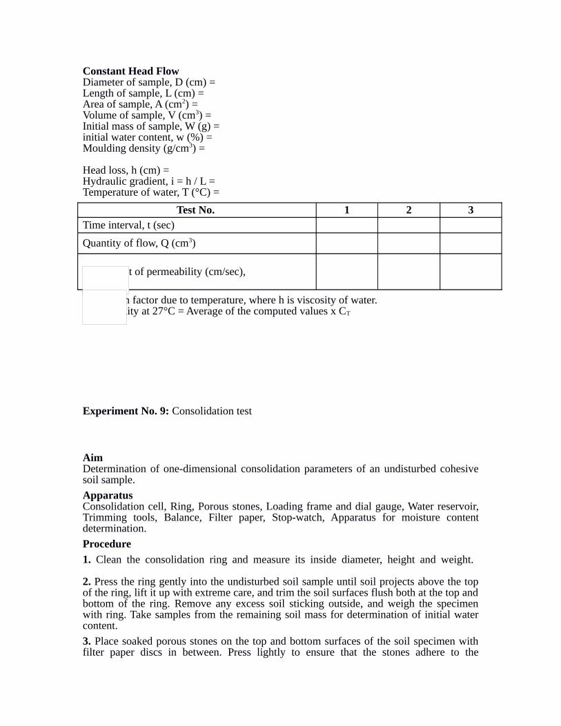
Table 2: Calculation of e, av and mv

Applied pressure

p (kg/cm2)

Final dial readings(mm)

Change in height of sample(mm)

Height of sample (mm)

Void ratio

Coefficientof

compressibility (cm2/kg)

1+e0

Coefficient of volume

compressibility(cm2/kg)

(1) (2) (3) (4) (5) (6) (7) (8) (9)0

0.1 0.2 0.4 0.8 1.6 3.2 6.4

1. Calculate the void ratio at the end of each pressure increment, and plot void ratio vs. pressure variation on simple graph paper. Determine coefficient of compressibility and coefficient of volume compressibility for each increment.

2. Plot void ratio vs. log pressure, and obtain compression index and preconsolidation stress (maximum past pressure).

3. For each pressure intensity, plot compression vs., and determine t90 by square root of time fitting method. Also construct a semilog plot of compression vs. time on log scale, and determine t50 by logarithm of time fitting method.

4. Calculate values of coefficient of consolidation (cv) for each pressure intensity applied to the specimen.

From square root of time fitting method,

From logarithm of time fitting method

,

Variable Head FlowDiameter of standpipe, d (cm) = Cross-sectional area of standpipe, a (cm2) =

Test No. 1 2 3Initial head, h1 (cm) Final head , h2 (cm) Time interval in seconds, ( t2 - t1)

Coefficient of permeability (cm/sec),

Permeability at 27°C = Average of the computed values x CT

Experiment No. 10: Direct shear test

Aim Determination of shear strength parameters of a silty or sandy soil at known density and moisture content.

ApparatusShear box with clamping screws, Box container, Porous stones, Grid plates (serrated and perforated), Tamper, Balance, Loading frame, Proving ring, Deformation dial gauges, Apparatus for moisture content determination.

Procedure

1. Measure shear box dimensions, set up the box by fixing its upper part to the lower part with clamping screws, and then place a porous stone at the base.

2. For undrained tests, place a serrated grid plate on the porous stone with the serrations at right angle to the direction of shear. For drained tests, use a perforated grid over the porous stone.

3. Weigh an initial amount of soil in a pan. Place the soil into the shear box in three layers and for each layer apply a controlled amount of tamping with a tamper. Place the upper grid plate, porous stone and loading pad in sequence on the soil specimen. Weigh the pan again and compute the mass of soil used.

4. Place the box inside its container and mount it on the loading frame. Bring the upper half of the box in contact with the horizontal proving ring assembly. Fill the container with water if soil is to be saturated.

5. Complete the assembly, remove the clamping screws from the box, and initialize the horizontal displacement gauge, vertical displacement gauge and proving ring gauge to zero.

6. Set the vertical normal stress to a predetermined value. For drained tests, allow the soil to consolidate fully under this normal load. Avoid this step for undrained tests.

7. Start the motor with a selected speed and apply shear load at a constant rate of strain. Continue taking readings of the gauges until the horizontal shear load peaks and then falls, or the horizontal displacement reaches 20% of the specimen length.

8. Determine the moisture content of the specimen after the test. Repeat the test on identical specimens under different normal stress values.

Observations and Calculations

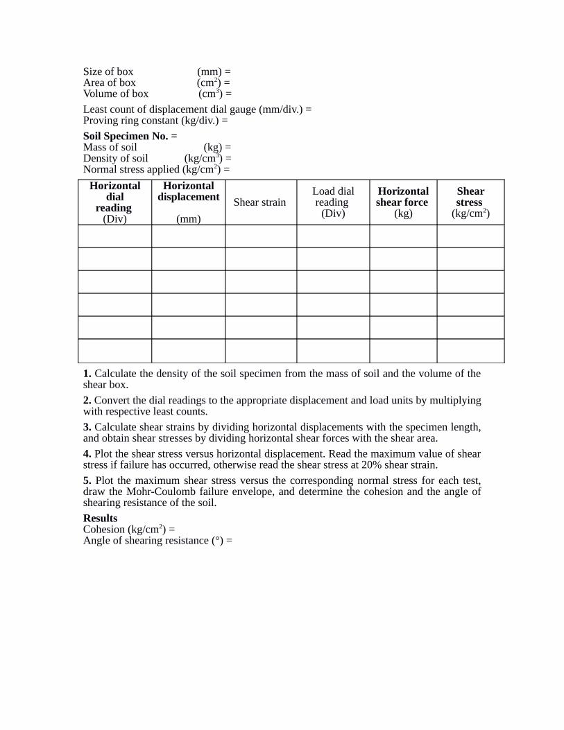
Size of box (mm) = Area of box (cm2) =Volume of box (cm3) =

Least count of displacement dial gauge (mm/div.) =Proving ring constant (kg/div.) =

Soil Specimen No. = Mass of soil (kg) = Density of soil (kg/cm3) = Normal stress applied (kg/cm2) =

Horizontal dial

reading (Div)

Horizontaldisplacement

(mm)

Shear strain Load dialreading

(Div)

Horizontal shear force

(kg)

Shearstress

(kg/cm2)

1. Calculate the density of the soil specimen from the mass of soil and the volume of the shear box.

2. Convert the dial readings to the appropriate displacement and load units by multiplying with respective least counts.

3. Calculate shear strains by dividing horizontal displacements with the specimen length, and obtain shear stresses by dividing horizontal shear forces with the shear area.

4. Plot the shear stress versus horizontal displacement. Read the maximum value of shear stress if failure has occurred, otherwise read the shear stress at 20% shear strain.

5. Plot the maximum shear stress versus the corresponding normal stress for each test, draw the Mohr-Coulomb failure envelope, and determine the cohesion and the angle of shearing resistance of the soil.

Results Cohesion (kg/cm2) = Angle of shearing resistance (°) =

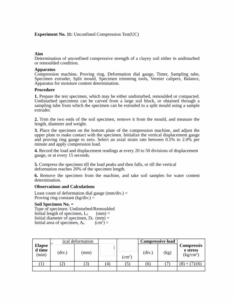
Experiment No. 11: Unconfined Compression Test(UC)

AimDetermination of unconfined compressive strength of a clayey soil either in undisturbed or remoulded condition.

ApparatusCompression machine, Proving ring, Deformation dial gauge, Timer, Sampling tube, Specimen extruder, Split mould, Specimen trimming tools, Vernier calipers, Balance, Apparatus for moisture content determination.

Procedure

1. Prepare the test specimen, which may be either undisturbed, remoulded or compacted. Undisturbed specimens can be carved from a large soil block, or obtained through a sampling tube from which the specimen can be extruded to a split mould using a sample extruder.

2. Trim the two ends of the soil specimen, remove it from the mould, and measure the length, diameter and weight.

3. Place the specimen on the bottom plate of the compression machine, and adjust the upper plate to make contact with the specimen. Initialize the vertical displacement gauge and proving ring gauge to zero. Select an axial strain rate between 0.5% to 2.0% per minute and apply compression load.

4. Record the load and displacement readings at every 20 to 50 divisions of displacement gauge, or at every 15 seconds.

5. Compress the specimen till the load peaks and then falls, or till the vertical deformation reaches 20% of the specimen length.

6. Remove the specimen from the machine, and take soil samples for water content determination.

Observations and Calculations

Least count of deformation dial gauge (mm/div.) =Proving ring constant (kg/div.) =

Soil Specimen No. = Type of specimen: Undisturbed/RemouldedInitial length of specimen, L0 (mm) = Initial diameter of specimen, D0 (mm) =Initial area of specimen, A0 (cm2) =

Elapsed time(min)

Vertical deformation

Vertical strain

Corrected area

(cm2)

Compressive loadCompressiv

e stress(kg/cm2)(div.) (mm) (div.) (kg)

(1) (2) (3) (4) (5) (6) (7) (8) = (7)/(6)

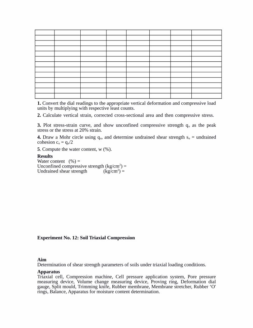
1. Convert the dial readings to the appropriate vertical deformation and compressive load units by multiplying with respective least counts.

2. Calculate vertical strain, corrected cross-sectional area and then compressive stress.

3. Plot stress-strain curve, and show unconfined compressive strength qu as the peak stress or the stress at 20% strain.

4. Draw a Mohr circle using qu, and determine undrained shear strength su = undrained cohesion cu = qu/2

5. Compute the water content, w (%).

ResultsWater content (%) =Unconfined compressive strength (kg/cm2) = Undrained shear strength (kg/cm2) =

Experiment No. 12: Soil Triaxial Compression

AimDetermination of shear strength parameters of soils under triaxial loading conditions.

ApparatusTriaxial cell, Compression machine, Cell pressure application system, Pore pressure measuring device, Volume change measuring device, Proving ring, Deformation dial gauge, Split mould, Trimming knife, Rubber membrane, Membrane stretcher, Rubber ‘O' rings, Balance, Apparatus for moisture content determination.

Procedure

1. Prepare a test specimen of necessary diameter and length, and measure its weight. Place a rubber membrane around the specimen using the membrane stretcher.

2. De-air the outlet line at the pedestal of the triaxial base, place on its top a saturated porous stone with a filter paper disc, and then position the soil specimen with the membrane stretcher around it. Put a loading cap on the specimen top, and seal the membrane on to the bottom pedestal and the top cap with ‘O' rings.

3. Assemble the triaxial cell with the loading ram initially clear of the top cap. Fill the cell with water, raise the water pressure to the desired value, and maintain the pressure constant. Raise the platform of the compression machine to bring the ram in contact with the seat on the top cap.

4. Set both the proving ring dial gauge and the deformation dial gauge to zero, select an axial strain rate, and verify that the cell pressure remains constant.

5. For undrained shearing of saturated samples, either close the outlet valve at the base of the cell or connect it to a pore pressure transducer. For drained shearing of saturated samples, connect the outlet to a burette for volume change measurements.

6. Apply axial compression load and take readings of the proving ring at intervals of 0.20 mm vertical deformation till the peak load has been passed, or till the strain reaches 20% of the specimen length. Record also burette or pore pressure readings, as applicable.

7. Remove the axial load, drain the water from the cell, remove the specimen, make a sketch of the failure pattern, and take soil samples for water content determination.

8. Repeat the test on identical soil specimens under different cell pressures.

Observations and Calculations

Least count of deformation dial gauge (mm/div.) = Proving ring constant (kg/div.) =

Soil Specimen No. = Confining cell pressure, (kg/cm2) = Initial diameter of specimen, D0 (mm) = Initial length of specimen, L0 (mm) = Initial area of specimen, A0 (cm2) = Initial volume of specimen, V0 (cm3) =

Deformation dial reading Vertica

lstrain

Burette

reading

(DV)(cm3)

Pore pressu

re change

(Du) (kg/cm

2)

Proving ring dial reading

Corrected area

for undrained test

(cm2)

Corrected area for drained

test

(cm2)

Deviatoric stress(kg/cm(div.) (mm) (div.) (kg)

(1) (2) (3) (4) (5) (6) (7) (8) (9) (10) = (7)/A

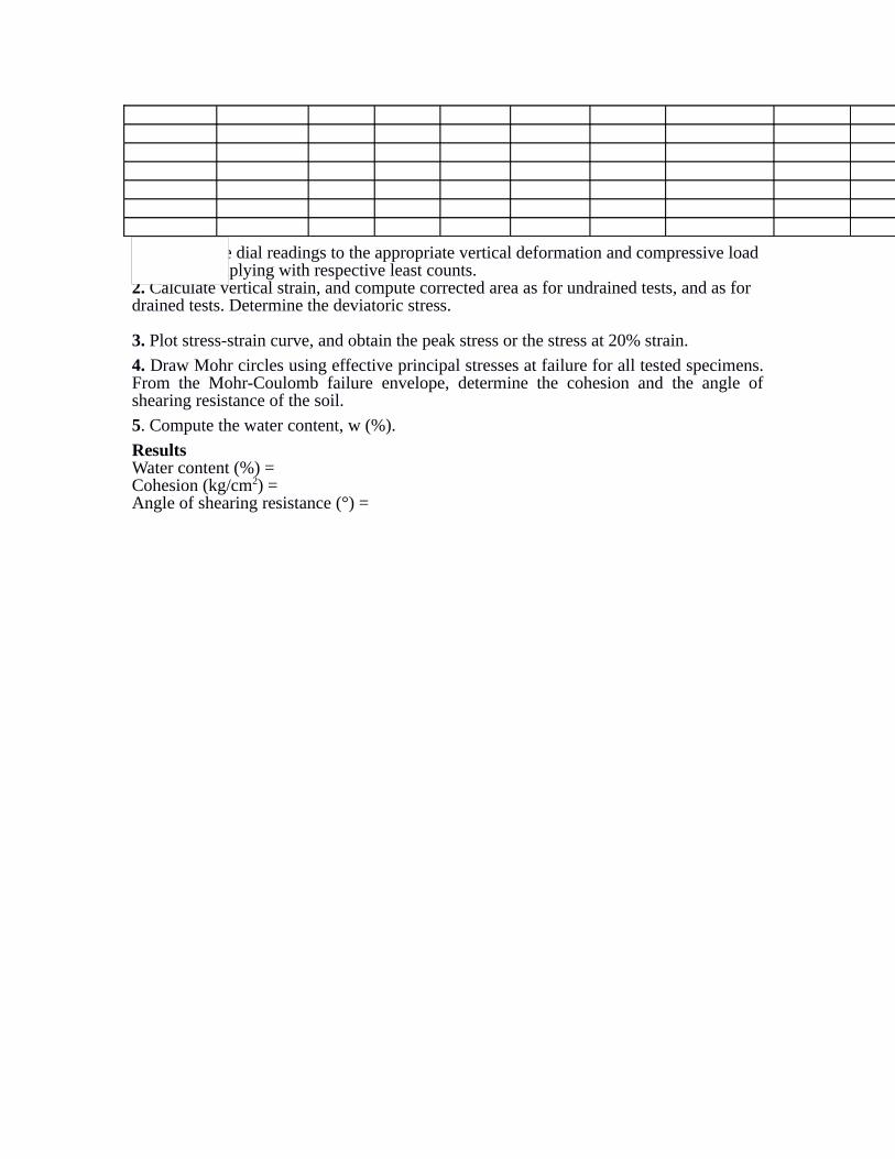
1. Convert the dial readings to the appropriate vertical deformation and compressive load units by multiplying with respective least counts.2. Calculate vertical strain, and compute corrected area as for undrained tests, and as for drained tests. Determine the deviatoric stress.

3. Plot stress-strain curve, and obtain the peak stress or the stress at 20% strain.

4. Draw Mohr circles using effective principal stresses at failure for all tested specimens. From the Mohr-Coulomb failure envelope, determine the cohesion and the angle of shearing resistance of the soil.

5. Compute the water content, w (%).

ResultsWater content (%) =Cohesion (kg/cm2) = Angle of shearing resistance (°) =