soil liquefaction response in mid-america...
TRANSCRIPT

Soil Liquefaction Response in Mid-America Evaluated
by Seismic Piezocone Tests
Mid-America Earthquake Center Report MAE-GT-3A
prepared by
James A. Schneider
and
Paul W. Mayne
Geosystems Program Civil & Environmental Engineering
Georgia Institute of Technology Atlanta, GA 30332
October 1999

ii
ACKNOWLEDGEMENTS
This project required the assistance of many individuals who are working on seismic
hazards in Mid-America, field testing, and geotechnical site investigation. Appreciation
is expressed to Dr. Buddy Schweig (USGS), Professor Martitia Tuttle (University of
Maryland), Professor Roy VanArsdale (University of Memphis), Joan Gomberg (USGS),
Marion Haynes (Blytheville, AR), Dr. Loraine Wolf (Auburn), Kevin McLain
(MODOT), Professor Tim Stark (UIUC), as well as other researchers at the Mid-America
Earthquake (MAE) Center and the Center for Earthquake Research and Information
(CERI). Particular gratitude is due to Professors Glenn J. Rix, J. David Frost, and J.
Carlos Santamarina at GT for their participation. Dr. Howard Hwang is thanked for
access to his database of boring logs and soil index properties from Memphis & Shelby
County. Dr. Bob Herrmann (St. Louis University) helped with the synthetic ground
motion program and site amplification parameters selection for Mid-America.
Fieldwork associated with this research was accomplished with the help of Ken
Thomas, Alec McGillivray, Tom Casey, Tracy Hendren, and Ethan Cargill of Georgia
Tech. Scott Olson (UIUC) and Brad Pemberton (Gregg In-Situ) are thanked for their
assistance in the New Madrid/MO and Charleston/SC seismic regions, respectively.
Laboratory resonant column tests performed by Brendan Sheppard and Dr. Laureano
Hoyos Jr. (GT) were also helpful.
Correspondence though e-mail and/or data sets provided by Professor Les Youd
(BYU), Dr. Ron Andrus (NIST), Dr. Ed Kavazanjian (GeoSyntec), Professor Ross
Boulanger (U.C.-Davis), Professor I.M. Idriss (U.C.-Davis), and others at the United
States Geologic Survey (USGS), have been helpful to provide additional perspective to
the issues associated with this study

vi
TABLE OF CONTENTS ACKNOWLEDGEMENTS iii LIST OF TABLES
ix
LIST OF FIGURES
xi
SUMMARY
xix
CHAPTER 1. INTRODUCTION 1.1 Motivation 1.2 Background on Soil Liquefaction 1.3 Scope CHAPTER 2. IN-SITU GEOTECHNICAL TESTING 2.1 Introduction
2.2 Standard Penetration Test 2.3 Cone Penetration Test
2.4 Seismic Piezocone Penetration Test 2.4.1 Shear Wave Velocity and Stiffness 2.4.2 Comparison of Penetrometers 2.4.3 Stress Normalization 2.4.4 Soil Classification 2.5 Summary and Reccommendations CHAPTER 3. SEISMIC HAZARDS AND GROUND MOTIONS IN MID-AMERICA 3.1 Seismic Hazards 3.1.1 New Madrid Seismic Zone 3.1.2 Charleston Seismic Region 3.2 Seismic Ground Hazard Analysis 3.3 Mid-America Deep Soil Models
3.4 Empirical Attenuation Relationships 3.5 Summary
CHAPTER 4. LIQUEFACTION RESPONSE OF SOILS 4.1 Overview 4.1 Cyclic Stress Approach 4.2.1 Stress Reduction Coefficient
1 1 2 8
10 10 10 12 18 21 27 29 35 41
43
43 45 47 47 54 64 70
73 73 74 75

vii
4.2.2 Magnitude Scaling Factors 4.2.3 Cyclic Resistance Ratio 4.2.4 Application to Paleoliquefaction Studies 4.2.5 Liquefaction Evaluation from Standard Penetration Test Data 4.2.6 Liquefaction Evaluation from Cone Penetration Test Data 4.2.7 Liquefaction Evaluation from Shear Wave Velocity Data 4.2.8 Extrapolation to High CSR 4.3 Cyclic Strain Approach 4.3.1 Shear Strain Level with Depth 4.3.2 Initial Porewater Pressure Generation 4.3.3 Cyclic Pore Pressure Generation from Normalized Curves 4.4 Arias Intensity Method 4.5 Summary
77 79 81 82 86 90 93 97 99
100 101 106 109
CHAPTER 5. GEOTECHNICAL SITE CHARACTERIZATION OF MID-AMERICA SOILS 5.1 Overview 5.2 Laboratory Index Testing 5.3 Seismic Piezocone Test Results 5.3.1 SCPTu Profiles 5.3.2 Site Variation 5.4 Summary
111
111 111 121 123 142 145
CHAPTER 6. ANALYSIS OF SOIL LIQUEFACTION RESPONSE USING SEISMIC CONE DATA 6.1 Overview 6.2 Critical Layer Selection 6.3 Cyclic Stress Based Methods 6.4 Arias Intensity Method 6.5 Cyclic Strain Based Method 6.6 Comparison of Methods
147
147 149 158 169 175 184
CHAPTER 7. CONCLUSIONS AND FUTURE WORK 7.1 Conclusions and Recommendations 7.2 Future Work
189 189 191
APPENDICES I. SOIL PROPERTIES I.1 Overview I.2 Soil Characterization and Basic Properties I.3 Consistency of Granular Materials I.4 Effective Stress State in Soils I.5 Strength Properties of Granular Materials
196 196 197 200 202 206

viii
I.6 Critical State Properties of Granular Materials I.7 Small Strain Properties II. GROUND MOTION PARAMETERS II.A Overview II.B Moment Magnitude II.C Peak Ground Acceleration II.D Arias Intensity III. SEISMIC PIEZOCONE DATA COLLECTION SYSTEM AND SHEAR WAVE VELOCITY ANALYSIS PROCEDURE III.A Cone Penetrometers and Field Testing III.B Seismic Piezocone Testing Procedures IV. TEST SITES AND SOUNDING LOCATIONS A. Areas Studied and Sounding Locations B. Memphis, TN Area 1. Shelby Farms 2. Shelby Farms Shooting Range 3. Houston Levee 4. Wolf River Boulevard Construction Site 5. North 2nd Street (Bell Properties) 6. Monopole Tower 7. Shelby Forest C. Northeast Arkansas and Southeast Missouri 1. Yarbro Excavation 2. Bugg 40 (Haynes-307) 3. 3MS617 (Sigmund Site) 4. Huey House 5. Johnson Farm 6. Dodd Farm 7. I-155 Bridge D. Charleston, South Carolina 1. Hollywood Ditch 2. Thompson Industrial Services
208 213
215 215 215 219 220
221
221 224
226 226 228 228 229 232 232 232 235 235 238 238 238 242 242 242 245 245 250 251 251
REFERENCES
254
ix
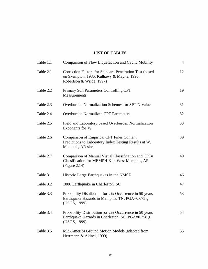
LIST OF TABLES
Table 1.1 Comparison of Flow Liquefaction and Cyclic Mobility
4
Table 2.1 Correction Factors for Standard Penetration Test (based on Skempton, 1986; Kulhawy & Mayne, 1990; Robertson & Wride, 1997)
12
Table 2.2 Primary Soil Parameters Controlling CPT Measurements
19
Table 2.3 Overburden Normalization Schemes for SPT N-value 31
Table 2.4 Overburden Normalized CPT Parameters 32
Table 2.5 Field and Laboratory based Overburden Normalization Exponents for Vs
33
Table 2.6 Comparison of Empirical CPT Fines Content Predictions to Laboratory Index Testing Results at W. Memphis, AR site
39
Table 2.7 Comparison of Manual Visual Classification and CPTu Classification for MEMPH-K in West Memphis, AR (Figure 2.14)
40
Table 3.1 Historic Large Earthquakes in the NMSZ 46
Table 3.2 1886 Earthquake in Charleston, SC 47
Table 3.3 Probability Distribution for 2% Occurrence in 50 years Earthquake Hazards in Memphis, TN; PGA=0.675 g (USGS, 1999)
53
Table 3.4 Probability Distribution for 2% Occurrence in 50 years Earthquake Hazards in Charleston, SC; PGA=0.758 g (USGS, 1999)
54
Table 3.5 Mid-America Ground Motion Models (adapted from Herrmann & Akinci, 1999)
55

x
Table 5.1 Grain Characteristics for Sands from Mid-America and Standard Reference Sands
120
Table 5.2 Seismic Piezocone Testing in Mid-America Earthquake
Region 124
Table 6.1 Sites and Associated Earthquakes 148
Table 6.2 Layer Parameters used for Simplified Analysis 156
Table 6.3 Seismic Piezocone Parameters used for Simplified Analysis
157
Table 6.4 Peak Ground Acceleration (g) for Earthquake Scenarios (M3 Model)
160
Table 6.5 Inferred Minimum Magnitude to Cause Liquefaction 185
Table 6.6 Comparison of Simplified Liquefaction Analysis Methods
186

xi
LIST OF FIGURES
Figure 1.1 Seismic Dual-Element Piezocone Penetrometer Indicating the Position and Direction of the Measurements
6
Figure 2.1 Setup and Equipment for the Standard Penetration Test (adapted from Kovacs et al., 1981)
11
Figure 2.2 Typical Boring Log from Shelby Forest, TN (Liu et al., 1997)
13
Figure 2.3 Types of Cone Penetrometers and Measurement Locations
15
Figure 2.4 Seismic Piezocone Probes used in this Study
15
Figure 2.5 Raw SCPTu data from Bell Properties, Memphis, TN
16
Figure 2.6 Seismic Piezocone Parameters used for Earthquake Analysis of Soil
20
Figure 2.7 Field and Laboratory Methods to Determine Shear Wave Velocity
23
Figure 2.8 Dynamic Properties from Seismic Piezocone Sounding at Shelby Farms, Shelby County, TN
24
Figure 2.9 Shear Modulus Reduction Schemes with Increasing Strain
26
Figure 2.10 Comparison of 5T (10 cm2), 10 T (10 cm2), and 15 T (15 cm2) Hogentogler electronic cones at 3MS617 Site (Blytheville, AR)
26
Figure 2.11 Comparison of u1 and u2 Piezocone Tests at I-155 Bridge (Caruthersville, MO)
28
Figure 2.12 Normalized Parameters from I-155 Bridge Data (Caruthersville, MO)
34
Figure 2.13 CPTu Soil Classification Charts (a) Robertson et al., 1986 (b) Robertson, 1990
36

xii
Figure 2.14 Olsen & Mitchell (1995) Normalized Classification Chart 37
Figure 2.15 Layering from SCPTu data at Monopole Tower (W. Memphis, AR)
38
Figure 3.1 Recent Seismicity (1975-1995) and Fault Structure in NMSZ (adapted from Schweig & VanArsdale, 1996; USGS & USNRC; http://www.eas.slu.edu/Earthquake_Center/ newmadrid1975-1995.html)
44
Figure 3.2 Comparison of Felt Areas for Similar Magnitude Earthquakes in California (Northridge; 1994) and Central United States (Charleston, MO; 1895)
45
Figure 3.3 Seismicity in Charleston, SC Earthquake Region 1698-1995 (http://prithvi.seis.sc.edu/images/Map5H.gif)
48
Figure 3.4 Graphical Representation of Distance to Site from Dipping Faults
49
Figure 3.5 Comparison of Hypocentral Depths for Mid-America and Western United States (data from Stover & Coffman, 1993)
50
Figure 3.6 Comparison of Acceleration at Soft Soil Sites to Rock Sites (Idriss, 1999)
56
Figure 3.7 Soil Column Depth-Dependent Shear Wave Velocity (Vs) Profile used in Herrmann & Akinci (1999) Soil Models (M3,M4,M5) (http://www.eas.slu.edu/People/RBHerrmann/ HAZMAP/hazmap.html)
58
Figure 3.8 Sediment Thickness Model of Mississippi River Valley (http://www.eas.slu.edu/People/RBHerrmann/HAZMAP/ hazmap.html)
59
Figure 3.9 Generalized Cross Section of Upper Mississippi River Valley (adapted from Whittenberg et al., 1977)
60
Figure 3.10 Generalized Cross Section of Charleston, SC Stratigraphy from Clubhouse Crossroads Borings (Adapted from Gohn et al., 1983)
60
Figure 3.11 Comparison of Accelerations Produced by Different Ground
Motion Models available for Mid-American Soils; Mw = 7.0 63

xiii
Figure 3.12 Effect of Soil Column Depth on PGA as Predicted by the Herrmann & Akinci (1999) Mid-America Deep Soil Model; Mw = 7.0
63
Figure 3.13 Comparison of Previously Proposed Attenuation Relationships for New Madrid Seismic Zone and Results of Modified USGS model (Mw = 7.0)
67
Figure 3.14 Comparison of Previously Proposed Attenuation Relationships for Charleston, SC EQ Region and Results of Modified USGS model (Mw = 7.0)
67
Figure 3.15 Comparison of Toro et al. (lines; 1997) and Modified USGS (points) model for NMSZ on semi- log scale (5.5<Mw<8.0)
68
Figure 3.16 Comparison of Toro et al. (lines; 1997) and Modified USGS (points) model for NMSZ on log- log scale (5.5<Mw<8.0)
68
Figure 3.17 Comparison of Toro et al. (lines; 1997) and Modified USGS (points) model for Charleston, SC on semi- log scale (5.5<Mw<8.0)
69
Figure 3.18 Comparison of Toro et al. (lines; 1997) and Modified USGS (points) model for Charleston, SC on log- log scale (5.5<Mw<8.0)
69
Figure 3.19 Comparison of Previously Reported Attenuation Relationships for New Madrid Seismic Zone and results of Modified USGS model (Mw = 7.0)
71
Figure 3.20 Comparison of Previously Reported Attenuation Relationships for Charleston, SC Earthquake Region and results of Modified USGS model (Mw = 7.0)
71
Figure 4.1 Stress Reduction Coefficients for Simplified Procedures 76
Figure 4.2 Effects of Revised Stress Reduction Coefficients on Magnitude Scaling Factors (Idriss, 1999 factors used for this study)
78
Figure 4.3 Key Aspects of Simplified Cyclic Stress Based Charts 80

xiv
Figure 4.4 SPT Liquefaction Site Database and NCEER CRR curves (a) FC (%) < 5; (b) 5 < FC (%) < 15; (c) 15 < FC (%) < 35; (d) FC (%) > 35 (adapted from Seed et al., 1985; Robertson & Wride, 1997)
85
Figure 4.5 CPT Liquefaction Database and NCEER Recommended CRR (a) Clean Sand; (b) Silty Sand; (c) Sandy Silt; (d) NCEER Curves (adapted from Olson & Stark, 1998; Robertson & Wride, 1997)
89
Figure 4.6 Vs Liquefaction Database and Recommended CRR Curves (a) Clean Sand; (b) Silty Sand; (c) Sandy Silt; (d) Andrus et al (1999) Curves (adapted from Andrus & Stokoe,1997; Andrus et al.,1999)
92
Figure 4.7 Comparison of CPT CRR curves and Laboratory Frozen Specimen Data
94
Figure 4.8 Comparison of Vs1 CRR curve and Laboratory Frozen Specimen Data
94
Figure 4.9 Comparison of CRR curves with CPT Field Performance Data
96
Figure 4.10 Density Independence of Initial Porewater Pressure Generation (after Ladd et al., 1989)
98
Figure 4.11 Sand Type and Preparation Method Independence of Porewater Pressure Generation (after Ladd et al.,1989)
98
Figure 4.12 Normalized Pore Pressure Generation Curves as a Function of Ko (adapted from Vasquez-Herrera et al., 1989)
105
Figure 4.13 Arias Intensity Liquefaction Field Data Compared to Curves form Kayen & Mitchell (1997) and Equation 4.28
108
Figure 5.1 Characteristic Values of Roundness (adapted from Youd, 1973)
114
Figure 5.2 Magnified View of Particles from Shelby Farms (SF) 115
Figure 5.3 Magnified View of Particles from Houston Levee (HL) 116

xv
Figure 5.4 Magnified View of Particles from Wolf River at Mississippi River (WRMS)
117
Figure 5.5 Magnified View of Particles form Yarbro Excavation (YE) 118
Figure 5.6 Grain Size Curves for Sands from Mid-America 119
Figure 5.7 Test areas presented on USGS 1996 2% PE in 50 years Central and Eastern United States Map; http://www.geohazards.cr.usgs.gov/eq/hazmaps/250pga.gif
122
Figure 5.8 General soil classification legend for profiles depicted 123
Figure 5.9 Seismic Piezocone Test Results from Shelby Farms, TN (MEMPH-G)
125
Figure 5.10 Seismic Piezocone Test Results from Shelby Farms Shooting Range, TN (SFSR-01)
126
Figure 5.11 Seismic Piezocone Test Results from Houston Levee, TN
(MEMPH-H) 127
Figure 5.12 Seismic Piezocone Test Results from Shelby Forset, TN (SFOR-01)
128
Figure 5.13 Seismic Piezocone Test Results from Yarbro Excavation, AR (YARB-01)
129
Figure 5.14 Seismic Piezocone Test Results from Bugg-40, AR (BUGG-01)
130
Figure 5.15 Seismic Piezocone Test Results from Bugg-40, AR (BUGG-02)
131
Figure 5.16 Seismic Piezocone Test Results from 3MS617, AR (3MS617-A)
132
Figure 5.17 Seismic Piezocone Test Results from Huey House, AR (HUEY-01)
133
Figure 5.18 Seismic Piezocone Test Results from Dodd Farm, MO (DODD-01)
134
Figure 5.19 Seismic Piezocone Test Results from Dodd Farm, MO (DODD-02)
135

xvi
Figure 5.20 Piezocone Test Results from Dodd Farm, MO (DODD-03) 136
Figure 5.21 Seismic Piezocone Test Results from Johnson farm, MO (JOHN-01)
137
Figure 5.22 Seismic Piezocone Test Results from Hollywood Ditch, SC (HW-4)
138
Figure 5.23 Seismic Piezocone Test Results from Thompson Industrial Services (TIS-1)
139
Figure 5.24 Typical Mississippi River Valley Cross Section in NE Arkansas and SE Missouri (Saucier, 1994) with Approximate Locations and Depths of Seismic Piezocone Soundings
141
Figure 5.25 Comparison of Site Variability at Dodd Farm 144
Figure 5.26 Site Variability at Bugg-40 145
Figure 6.1 Mechanical Cone Resistance in Loose Layers at a Site of Re-Liquefaction in Brawley, California (Youd, 1984)
151
Figure 6.2 Normalization of Uniform Loose and Dense Sand Layers at Huey House, Blytheville, AR (log- log stress scale)
153
Figure 6.3 Normalization of Uniform Loose and Dense Sand Layers at Huey House, Blytheville, AR (based on standard plotting scales)
153
Figure 6.4 Ten Critical Layers Selected for Liquefaction Analysis 154
Figure 6.5 Twelve Critical Layers Selected for Liquefaction Analysis 155
Figure 6.6 Key Aspects of Cyclic Stress Based analysis Charts for this Study
161
Figure 6.7 Cyclic Stress based analysis for 800-1000 New Madrid Earthquake (a) qt1N; repi = 15 km; (b) Vs1; repi = 15 km; (c) qt1N; repi = 25 km; (d) Vs1; repi = 25 km
163
Figure 6.8 Cyclic Stress based analysis for 1400-1600 New Madrid Earthquake (a) qt1N; repi = 15 km; (b) Vs1; repi = 15 km; (c) qt1N; repi = 25 km; (d) Vs1; repi = 25 km
164

xvii
Figure 6.9 Cyclic Stress based analysis for December 1811 New
Madrid Earthquake (a) qt1N; (b) Vs1; 165
Figure 6.10 Cyclic Stress based analysis for January 1812 New Madrid Earthquake (a) qt1N; (b) Vs1;
166
Figure 6.11 Cyclic Stress based analysis for February 1812 New Madrid Earthquake (a) qt1N; (b) Vs1;
167
Figure 6.12 Cyclic Stress based analysis for September 1886 Charleston,SC Earthquake (a) qt1N; (b) Vs1;
168
Figure 6.13 Key Aspects of Arias Intensity Based analysis Charts for this Study
170
Figure 6.14 Arias Intensity based analysis for 800-1000 New Madrid Earthquake (a) qt1N; repi = 15 km; (b) qt1N; repi = 25 km
171
Figure 6.15 Arias Intensity based analysis for 1400-1600 New Madrid
Earthquake (a) qt1N; repi = 15 km; (b) qt1N; repi = 25 km` 172
Figure 6.16 Arias Intensity based analysis for December 1811 New Madrid Earthquake (qt1N)
173
Figure 6.17 Arias Intensity based analysis for January 1812 New Madrid Earthquake (qt1N)
173
Figure 6.18 Arias Intensity based analysis for February 1812 New Madrid Earthquake (qt1N)
174
Figure 6.19 Arias Intensity based analysis for September 1886 Charleston,SC Earthquake (qt1N)
174
Figure 6.20 Key Aspects of Cyclic Strain Based analysis Charts for this Study
177
Figure 6.21 Cyclic Strain based analysis for 800-1000 New Madrid
Earthquake (a) qt1N; repi = 15 km; (b) Vs1; repi = 15 km; (c) qt1N; repi = 25 km; (d) Vs1; repi = 25 km
178
Figure 6.22 Cyclic Strain based analysis for 1400-1600 New Madrid Earthquake (a) qt1N; repi = 15 km; (b) Vs1; repi = 15 km; (c) qt1N; repi = 25 km; (d) Vs1; repi = 25 km
179

xviii
Figure 6.23 Cyclic Strain based analysis for December 1811 New Madrid Earthquake (a) qt1N; (b) Vs1;
180
Figure 6.24 Cyclic Strain based analys is for January 1812 New Madrid Earthquake (a) qt1N; (b) Vs1;
181
Figure 6.25 Cyclic Strain based analysis for February 1812 New Madrid Earthquake (a) qt1N; (b) Vs1;
182
Figure 6.26 Cyclic Strain based analysis for September 1886 Charleston,SC Earthquake (a) qt1N; (b) Vs1;
183
Figure 6.27 Comparison of Lower Bound Magnitude Required for Liquefaction to Previous Estimates of Moment Magnitude (NMSZ)
187
Figure 7.1 Ground Motions and Seismic Analysis in Mid-America 192
Figure 7.2 Static piezovibrocone andseismic Piezocone soundings at Hollywood Ditch, Charleston, SC
194
Figure 7.3 Comparison of static and dynamic piezovibrocone soundings at Hollywood Ditch, Charleston, SC
194

xix
SUMMARY
The Mid-America earthquake region is now recognized as containing significant
seismic hazards from historically- large events that were centered near New Madrid, MO
in 1811 and 1812 and Charleston, SC in 1886. Large events prior to these times are also
acknowledged. Methods for evaluating ground hazards as a result of soil liquefaction and
site amplification are needed in order to properly assess risks and consequences of the
next seismic event in these areas. In-situ tests provide quick, economical, and practical
means for these purposes. The seismic piezocone penetration test (SCPTu) is a hybrid in-
situ test method, which provides downhole measurements of shear wave velocity in
addition to penetration test parameters within a single vertical sounding. The SCPTu
provides four independent readings that can be used for soil classification, site
amplification analysis, direct liquefaction analysis, as well estimation of soil properties
for a rational engineering assessment of soil liquefaction.
For this research effort, in-situ penetration tests have been performed at a number
of test sites in the heart of the Mid-America earthquake regions. Testing areas include
Charleston SC, Memphis TN, West Memphis AR, Blytheville AR, Steele MO, and
Caruthersville, MO. Many of these sites have already been associated with liquefaction
features such as sand dikes, sand boils, or subsidence, observed during geologic and
paleoseismic studies. Seismic piezocone penetration tests have been performed in these
localities. Data collected at these sites have been analyzed under current methodologies

xx
to assess the validity of empirical relations developed for Chinese, Japanese, and
Californian interplate earthquakes when applied to historical Mid-American earthquakes.
Simplified cyclic strain theory will be combined with empirical estimation of soil
properties to evaluate pore pressure generation and liquefaction potential.
Evaluation of liquefaction response of soils is complicated in Mid-America due to
the deep soil columns of the Mississippi River Valley and Atlantic Coastal plain,
infrequency of large events needed for calibration of models and analysis techniques, and
uncertainty associated with the mechanisms and subsequent motions resulting from
intraplate earthquakes. These aspects of Mid-America earthquakes have been considered
in analyses conducted for this study.
Six earthquake events in Mid-America have been evaluated using four separate
types of analyses on 22 critical layers from 12 sites. The results of these analyses
indicate that:
• current methods generally agree in the prediction of liquefaction at a site;
• modulus reduction schemes used in cyclic strain based procedures tend to bridge the
gap between the small strain measurement of shear wave velocity and large strain
phenomena of liquefaction; and
• liquefaction may have occurred throughout the thickness of the soil deposits
analyzed.
• The use of attenuation relationships which do not account for the non- linear nature of
soil deposits adds uncertainty to these results and remains the subject of additional
research.
1
CHAPTER 1
INTRODUCTION
1.1 Motivation
It is now recognized that several of the largest historical earthquake events in the
United States occurred in the New Madrid, MO area during 1811 and 1812, and in
Charleston, SC in 1886. The New Madrid series of 1811-1812 consisted of over 200
separate seismic events, which would have created an equivalent single event with a
moment magnitude (Mw; Appendix II) of about 8.3 (Johnston & Schweig, 1996). The
three largest individual events of the series were estimated to have moment magnitudes
of about 7.9, 7.6, and 8.0 on December 16, 1811, January 23, 1812, and February 7, 1812
respectively (Johnston & Schweig, 1996). The Charleston, SC earthquake consisted of a
single event on September 1, 1886, with a Mw estimated at 7.0 (Stover & Coffman,
1993).
Ongoing research on the magnitude, attenuation, and recurrence of earthquake
events in Mid-America has led to the increased awareness of the potential for serious
ground failures in the New Madrid, MO seismic zone and Charleston, SC earthquake
region. Strong ground motions can lead to injury and death from damaged structures,
primarily from the collapse of buildings and bridges. Site amplification and liquefaction-
induced ground failures may increase the severity of earthquake effects. Large lateral

2
and vertical movements will rupture pipelines and utilities, crippling lifeline facilities
needed to provide aid and relief to the injured.
It will be desirable to evaluate the response of soils to earthquake shaking and
potential for liquefaction in an expedient and cost effective manner in the Central and
Eastern United States (CEUS). However, the evaluation of liquefaction response of soils
is complicated in Mid-America due to the:
• deep vertical soil columns (600 m to 1400 m) of the Mississippi River Valley and
Atlantic Coastal plain;
• infrequency of large events needed for calibration of models and analysis techniques
(most recent severs events, Mw > 6.5, more than 100 years ago);
• uncertainty associated with the mechanisms and subsequent motions resulting from
intraplate earthquakes (e.g., California earthquakes are interplate events).
1.2 Background on Soil Liquefaction
Liquefaction is the result of excess porewater pressure generated in saturated granular
soils from rapid loading, and is often associated with earthquake shaking. Since soil
strength is proportional to the effective vertical stress (σvo'; Appendix I), the reduction of
effective stress from increased pore pressures (u) will lead to strength loss in a soil
deposit. The porewater pressure in the soil will be a combination of initial in-situ
porewater stress (uo) and the shear induced porewater pressure (∆u). When the pore
water pressure (u = ∆u + uo) equals the total overburden stress (σvo), the effective stress
(σvo' = σvo - u) will go to zero causing initial liquefaction (Seed & Lee, 1966).

3
The engineering terminology used to describe soil liquefaction is varied, so an
overview of definitions as discussed in Kramer (1996) and Robertson and Wride (1997)
will be presented here. There are two main terms that can be used to describe soil
liquefaction: flow liquefaction and cyclic softening. These terms are distinguished in
Table 1.1. Cyclic softening can be separated into cyclic liquefaction as well as cyclic
mobility. This study focuses specifically on cyclic liquefaction at sites with level ground.
Initial studies of liquefaction involved stress-controlled laboratory tests of
reconstituted specimens (Seed & Lee, 1966). Since the effects of structure, aging,
cementation, and strain history cannot be replicated in these specimens, the use of in-situ
testing results and field performance data has become a popular means of assessing
liquefaction susceptibility. Penetration resistance at sites where surface manifestations of
liquefaction were or were not evident have been compared to evaluate cyclic soil
resistance. Databases consisting predominantly of sites from China, Japan, and
California are available for the Standard Penetration Test (SPT; e.g., Seed et al., 1983),
cone penetration test (CPT; e.g., Olson & Stark, 1998), flat dilatometer test (DMT; e.g.,
Reyna & Chameau, 1991), and shear wave velocity (Vs; Andrus et al., 1999). Analyses
by these methods are considered as direct methods for liquefaction assessment of soils.
Estimation of soil properties using in-situ tests (e.g., Kulhawy & Mayne, 1990) and
incorporating these results into a theoretical framework for analysis can be considered an
indirect, yet rational, method for soil liquefaction assessment. Some theoretical
frameworks for liquefaction assessment that currently are in use include the cyclic-strain
based method (Dobry et al., 1982), nonlinear effective stress-based analyses (e.g., Finn et

4
al., 1977), and the critical-state approach for sands (e.g., Jefferies, 1999). Computer
models have been developed which incorporate these theories, and it should be noted that
the accuracy of the model prediction will only be as reliable and meaningful as the values
of input parameters.
Table 1.1. Comparison of Flow Liquefaction and Cyclic Mobility
Cyclic Softening
Flow Liquefaction Cyclic Liquefaction Cyclic Mobility
Loading Conditions Static or Cyclic Cyclic with stress reversal1
Cyclic without stress reversal1
Drainage Undrained Undrained Undrained Soil Response to
Shear (Appendix I) Strain Softening Strain Softening and
Strain Hardening Strain Softening and
Strain Hardening Controlling
Stresses Static Shear Stress Static and Cyclic
Shear Stresses Static and Cyclic
Shear Stresses Induced
Stress State In-situ shear stresses greater than minimum undrained shear strength
Effective stress state reaches essentially zero
Zero effective stress does not develop
Failure or Deformation
Potential
Sufficient volume of soil must strain soften. Failure can result in slide or flow depending upon internal geometry and stress state.
Strain softened shear modulus can lead to large deformations during cyclic loading. Soils will tend to stabilize upon termination of cyclic loading.
Limited deformations, unless very loose soil results in flow liquefaction.
Soil Types Any metastable saturated soil; very loose granular deposits, very sensit ive clays, and loess deposits
Almost all saturated sands, with limited deformations in clayey soils.
Almost all saturated sands, with limited deformations in clayey soils.
1 Stress reversal - during cyclic loading, the shear stresses alternate from positive to negative.

5
The significance of local site conditions and amplification of ground motions have
received increased recognition since the 1985 Mexico City and 1989 Loma Prieta
earthquakes (Kramer, 1996). Therefore, the use of computer codes for site-specific
cyclic stress-, cyclic strain-, or effective stress-based analysis may be necessary.
Commercially available software packages fall into the categories of equivalent linear 1-
D programs (e.g., SHAKE; Schnabel et al., 1972), true non- linear programs (e.g.,
DESRA; Lee & Finn, 1978), or equivalent linear 2-D programs (e.g., QUAD4; Idriss et
al., 1973). Analyses of sites at low peak ground accelerations (PGA < 0.4 g; Appendix
II) can commonly be achieved using equivalent linear 1-D codes. Large strains generated
by high peak ground accelerations (PGA > 0.4) from an extreme event may require
analysis by a 1-D true nonlinear program or a 2-D equivalent linear program to account
for additional complexities at individual sites.
To obtain parameters for engineering analysis and model studies, field test data are
necessary. The seismic piezocone penetrometer is an electronic probe that rapidly
provides four independent parameters to assess the subsurface profile with depth at an
individual site. Figure 1.1 depicts a seismic piezocone sounding, and displays the
location of tip resistance (qc), sleeve friction (fs), porewater pressure measurement (um),
and horizontal geophone for determining shear wave velocity (Vs). The tip resistance can
be used for a direct empirical analysis of soil liquefaction potential. Tip resistance can
also be used to evaluate effective stress friction angle (φ'), overconsolidation ratio (OCR),
in-situ coefficient of horizontal stress (Ko), or relative density (DR ) for an indirect, yet
rational analysis of soil behavior during seismic loading. Sleeve friction measurements

6
Figure 1.1. Seismic Dual-Element Piezocone Penetrometer Indicating the Position and Direction of the Measurements
fs
qc
Vs
u1
u2
Hydraulically Pushed at 20 mm/sec
Provides Four Independent Readings with Depth: Tip Resistance, qc ! qt (corrected)
Sleeve Friction, fs Pore Water Pressure, um
u2 (shoulder) u1 (midface)
Shear Wave Velocity, Vs (downhole)
60o
7
can be used for stratigrafic profiling and as an estimate of fines content necessary for
both direct and indirect methods. Porewater pressure, um, can be used for stratigraphic
profiling, as well as for the determination of groundwater table in sands and the stress
history of clays. Penetration porewater pressure dissipation tests can provide information
of the flow characteristics of the localized strata, including the coefficient of
consolidation (cv) and permeability (k). The shear wave velocity (Vs) is measured with a
horizontal geophone located about 25 cm behind the cone tip. Measurements are taken at
1-m depth intervals, so the downhole Vs is an averaged property over discrete depths.
Shear wave velocity can be used for direct liquefaction analysis through simplified
charts. Rational indirect analyses can be enhanced from the measurement of soil
stiffness, or evaluations of void ratio (e), and total mass density (ρtot).
Before an earthquake analysis can be performed, critical ground motion parameters
must be selected. An assessment of ground motion hazards is difficult in the Mid-
America earthquake region due to the lack of strong earthquakes in recent historical times
(t ≈ 100+ years), and lack of recorded data from the limited events that have occurre. For
seismic hazard analysis, probabilistic hazard information is available through the USGS
web site at (http://www.geohazards.cr.usgs.gov/eq). A stochastic ground motion model
has been under development for the Central and Eastern United States (CEUS), and
attenuation relationships have been determined utilizing this model (e.g., Toro et al.,
1997). Synthetic ground motions based on a representative stiffness profile of the
Mississippi River Valley deep soil column are still under development for the Mid-
America region (Herrmann & Akinci, 1999) at the time of this writing.

8
1.3 Scope
The purpose of this project is to assess the liquefaction response of Mid-American
soils. The use of in-situ testing methods and their application to geotechnical earthquake
engineering will be reviewed. Current and evolving methods for liquefaction assessment
will be discussed, with an emphasis on their use in Mid-America. There is a great deal of
uncertainty in assessing appropriate earthquake parameters for the Central and Eastern
United States (CEUS) due to the deep soil column over bedrock (600 m < z < 1400 m),
and infrequency of large events (f ≈ 250 years). Attenuation models for rock sites are
reviewed and compared to a recent deep soil model developed specifically for Mid-
America.
Seismic piezocone testing and limited surface sampling have been performed at a
number of sites across the New Madrid Seismic zone and Charleston, SC earthquake
region. The majority of these sites are historic liquefaction sites, having shown
indisputable evidence of sand boils, sand dikes, subsidence, and other geologic
liquefaction features. Data from index, laboratory, and field testing will be presented. To
assess soil liquefaction potential in Mid-America, the collected data will be incorporated
into a number of frameworks including:
• direct cyclic stress methods for cone tip resistance and shear wave velocity;
• direct Arias intensity method for cone tip resistance;
• evaluation of soil properties and input into cyclic strain-based theory.

9
Conclusions emanating from these studies will be derived and recommendations for
future work will be proposed to improve research and practice in Mid-America.

10
CHAPTER 2
IN-SITU GEOTECHNICAL TESTING
2.1 Introduction
Traditional means of geotechnical exploration of soil deposits consists of rotary
drilling techniques to generate soil borings. From these procedures, auger cuttings, drive
samples, and pushed tubes may be recovered. During the process of drive sampling, the
number of blows of a drop weight advancing a hollow pipe a given distance provides a
crude index of soil consistency. This procedure can be called an in-situ test. Modern
electronics have permitted advances in cone penetration test technology, allowing for
increased resolution with depth and more repeatable results. Enhanced in-situ tests have
incorporated additional sensors such as piezometers, geophones, as well as measurements
of electromagnetic properties such as resistivity and dielectric permittivity. This chapter
will provide background on in-situ testing, including the Standard Penetration Test
(SPT), the cone penetration test (CPT), with special emphasis on the seismic piezocone
test (SCPTu) and its application to geotechnical site characterization will be discussed.
2.2 Standard Penetration Test (SPT)
The standard penetration test (SPT) has been the most commonly-used in-situ test in
geotechnical subsurface investigations (Decourt et al., 1988). The test obtains both a
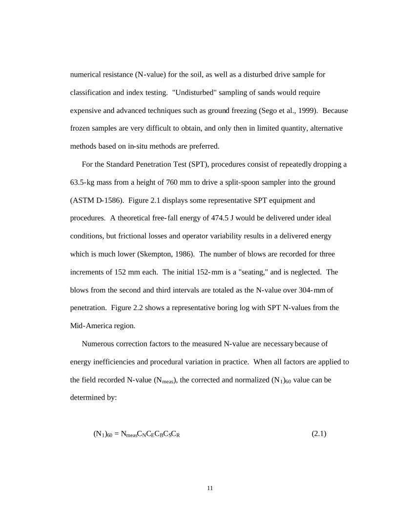
11
numerical resistance (N-value) for the soil, as well as a disturbed drive sample for
classification and index testing. "Undisturbed" sampling of sands would require
expensive and advanced techniques such as ground freezing (Sego et al., 1999). Because
frozen samples are very difficult to obtain, and only then in limited quantity, alternative
methods based on in-situ methods are preferred.
For the Standard Penetration Test (SPT), procedures consist of repeatedly dropping a
63.5-kg mass from a height of 760 mm to drive a split-spoon sampler into the ground
(ASTM D-1586). Figure 2.1 displays some representative SPT equipment and
procedures. A theoretical free-fall energy of 474.5 J would be delivered under ideal
conditions, but frictional losses and operator variability results in a delivered energy
which is much lower (Skempton, 1986). The number of blows are recorded for three
increments of 152 mm each. The initial 152-mm is a "seating," and is neglected. The
blows from the second and third intervals are totaled as the N-value over 304-mm of
penetration. Figure 2.2 shows a representative boring log with SPT N-values from the
Mid-America region.
Numerous correction factors to the measured N-value are necessary because of
energy inefficiencies and procedural variation in practice. When all factors are applied to
the field recorded N-value (Nmeas), the corrected and normalized (N1)60 value can be
determined by:
(N1)60 = NmeasCNCECBCSCR (2.1)

12
where correction factors are presented in Table 2.1 and include the effects of stress level
(CN), energy (CE), borehole diameter (CB), sampling method (C S), and rod length (CR).
In practice, the N-value is typically only corrected for overburden stress (CN), and the
energy efficiency is assumed to be 60 percent in the United States. Seed et al. (1985)
reviewed typical hammer energy efficiency around the world, and Farrar (1998)
performed a review of SPT energy measurements for a number of different SPT systems
in North America. For liquefaction studies it is recommended that energy efficiency
measurements be performed (ASTM D6066) to apply the correction factor (CE). The
additional correction factors for particle size (CP), aging (CA), and overconsolidation
(COCR), are presented, but these particular corrections are usually used only in research
studies and improved interpretations.
The overall effect of having so many corrections, each with its own great uncertainty,
is that little confidence can be assigned to the SPT as a reliable means for assessing the
liquefaction potential of soils. Due to these compounding errors, much interest has been
directed to the use of alternative in-situ test methods for evaluating seismic ground
response. The electronic cone penetrometer offers some clear advantages in this regard.
2.3 Cone Penetration Test (CPT)
Originally, a cone penetrometer was a mechanical device that produced tip stress
measurements with depth, with later adaptations for a sleeve resistance (Broms & Flodin,
1988). The probe is hydraulically pushed into the ground without the need for a soil
boring. The test equipment has evolved to its current state of electric and electronic cone

11
Figure 2.1. Setup and Equipment for the Standard Penetration Test (SPT) (adapted from Kovacs et al., 1981)
Fall Height: 760 mm
63.5 kg Mass
Drill Rod
Anvil
Drive Length: 456 mm
Split Spoon Sampler
d = 50 mm L > 600 mm
Hollow Stem Augers or Mud Filled Boring
Rotating Cathead
Pulley
Ground Surface
Split Spoon with Drive Sample
One or two wraps permitted by ASTM D1586 (3 or 4wraps sometimes used in the field)
SPT Hammer

12
Table 2.1. Correction Factors for Standard Penetration Test (based on Skempton, 1986; Kulhawy & Mayne, 1990; Robertson & Wride, 1997)
Effect
Variable
Term
Value
Overburden Stress
σvo' CN (Pa/σvo')0.5 but < 2
Energy Ratio1
• Safety Hammer • Donut Hammer • Automatic Hammer
CE 0.6 to 0.85 0.3 to 0.6 0.85 to 1.0
Borehole Diameter
• 65 to 115 mm • 150 mm • 200 mm
CB 1.00 1.05 1.15
Sampling Method
• Standard sampler • Sampler without liner
CS 1.0 1.1 to 1.3
Rod Length
• 10 m to 30 m • 6 to 10 m • 4 to 6 m • 3 to 4 m
CR 1.0 0.95 0.85 0.75
Particle Size
Median Grain Size (D50) of Sand in mm
CP 60 + 25 log D50
Aging
Time (t) in years since deposition
CA 1.2 + 0.05 log (t/100)
Overconsolidation
OCR COCR OCR0.2
1 Obtain by energy measurement per ASTM D4633

13
Figure 2.2. Typical Boring Log from Shelby Forest, TN (Liu et al., 1997)

14
penetrometers with standard readings of tip resistance (qc) and sleeve friction (fs), as
shown in Figure 2.3.a. The readings are collected by computerized data acquisition
systems converting analog signals from strain gauges to digital data. New sensors have
been added to cone penetrometers including pore pressure transducers with porous filters
located at the shoulder (Fig. 2.3.b.) or midface (Fig 2.3.c.) in order to measure
penetration porewater pressures (u2 or u1 respectively). Moreover, by incorporating
velocity geophones and a surface source, the shear wave arrival time (ts) can be recorded
with depth. Testing with this probe is known as the seismic piezocone penetration test
(SCPTu) as detailed by Campanella (1994). Figure 2.5 presents raw data from a SCPTu
sounding in Memphis, TN showing the four independent measured readings with depth;
qc, fs, u2, and ts. The four characteristic shear wave arrival times (first arrival, first
trough, crossover, and first peak) are described in Appendix III. This site is near areas of
historic liquefaction features with prior geologic evidence of sand dikes projecting
through overlying clayey silt stratum along the banks of the Wolf River near Mud Island
(personal communication, R. VanArsdale, 1998). Additionally, an inclinometer may be
installed in the cone to assess the verticality of the sound ing to warn against excessive
drift andpossible rod buckling. Figure 2.4 shows a photograph of the three seismic
piezocones used during this study, including 5-tonne, 10-tonne, and 15-tonne probes.
Standard cone penetrometers have a 60o apex at the tip, 10-cm2 projected tip area,
35.7 mm diameter, and 150-cm2 sleeve surface area. Cone penetrometers may also have
a 60o apex at the tip, 15-cm2 projected tip area, 44 mm diameter, and either 200- or 225-
cm2 sleeve surface area. The maximum capacity of the load cells may vary, with lower

15
60o
fs
qc
u2
60 o
fs
qc
60o
fs
qc
u1
60o
fs
qc
u2
Vs
Figure 2.3. Types of Cone Penetrometers and Measurement Locations: a. Electric Cone Penetrometer, CPT; b. Piezocone Penetrometer (filter behind tip), CPTu2;
c. Piezocone Penetrometer (mid-face filter) CPTu1; d. Seismic Piezocone, SCPTu2;
Hogentogler 5 T, 10 cm2 dual element seismic piezocone
Hogentogler 10 T, 10 cm2 u2 seismic piezocone
Hogentogler 15 T, 15 cm2 u2 seismic piezocone
Figure 2.4. Seismic Piezocone Probes used in this Study (quarter for scale)
a. b. c. d.

16
Figure 2.5. Raw SCPTu data from Bell Properties, Memphis, TN
capacity load cells providing higher resolution necessary for investigations in low
resistance soils, such as soft clays. The location of piezocone filters for pore pressure
measurement may be at mid-face (u1) and/or behind the shoulder (u2), as seen in Figure
2.3. Differences in penetrometer size, capacity, and pore pressure filter location will be
discussed further in Section 2.4.2 on the comparison of penetrometers.
Test procedures consist of hydraulically pushing the cone at a rate of 2 cm/s (ASTM
D5778) using either a standard drill rig or specialized cone truck. The advance of the
probe requires the successive addition of rods (either AW or EW drill rods or specialized
cone rods) at approximately 1 m or 1-5 m intervals. Readings of tip resistance (qc),
sleeve friction (fs), inclination (i), and pore pressure (um) are taken every 5-cm (2.5-sec).
Depending upon limitations of the data acquisition system, the readings may be recorded
0
5
10
15
0 10 20 30 40
qt (MPa)D
epth
BG
S (
m)
0
5
10
15
0 25 50 75 100
ts (msec)
First Arrival
FirstTroughCrossover
First Peak
0
5
10
15
0 100 200 300 400
fs (kPa)
0
5
10
15
-100 200 500 800
u2 (kPa)

17
at higher sampling rates to distinguish variations in soil strata, fabric, and layering. Shear
wave arrival times (ts) are typically recorded at rod breaks corresponding to 1-m
intervals. More information on cone penetration test procedures and equipment can be
found in Appendix III.
The cone tip resistance (qc) is the measured axial force over the projected tip area. It
is a point stress related to the bearing capacity of the soil. In sands, the tip resistance is
primarily controlled by the effective stress friction angle (φ'), relative density (Dr), and
effective horizontal stress-state (σho'). For intact clays, the tip resistance is primarily
controlled by the undrained shear strength (su). Particularly in clays and silts, the
measured qc must be corrected for porewater pressures acting on the cone tip geometry,
thus obtaining the corrected tip stress, qt (Lunne, et al., 1997):
qt = qc + (1-an)u2 (2.2)
where an is the net area ratio determined from laboratory calibration (Appendix III) and
u2 is the shoulder penetration porewater pressure. A general rule of thumb is that qt > 5
MPa in sands, while qt < 5 MPa in clays and silts.
The sleeve friction (fs) is determined as an axial load acting over the area of a smooth
sleeve. This value is typically expressed as the Friction Ratio (FR = fs / qt x 100), which
is indicative of soil type (Lunne et al., 1997). Often, FR< 1% in clean sands and FR > 4
% in clays and silts.

18
The penetration porewater pressures are monitored using a transducer and porous
filter element. The filter element position can be located mid-face on the cone (u1) or
behind the cone tip at the shoulder (u2), with the latter required for the correction of tip
resistance. These readings represent the fluid pressures between the soil particles. At the
shoulder position, the pressures are near hydrostatic in sands (u2 ≈ uo) whilst considerably
higher than hydrostatic (u2 > uo) in soft to firm to stiff intact clays. The pore pressure
parameter, Bq = (u2 - uo) / (qt - σvo), has been developed as a means to normalize CPTu
data for the purpose of soil classification and undrained shear strength estimation
(Senneset et al., 1982; Wroth, 1984). At the mid-face location (u1), penetration porewater
pressures are always positive, while at the u2 location measurements are either positive in
intact materials or negative in fissured soils (Mayne et al., 1990).
2.4 Seismic Piezocone Penetration Test (SCPTu)
Seismic cone penetration systems provide rapid, repeatable, near continuous,
measurements of multiple parameters that can be used to assess soil properties. To
analyze earthquake hazards, an understanding of each soil behavioral parameter available
from various cone penetration tests is necessary. Available measurements from seismic
cone penetrometers along with controlling parameters are presented in Table 2.2. With
regards to liquefaction evaluation, the individual recordings from seismic piezocone
penetration tests (SCPTu) can be valuable in evaluating input parameters as illustrated by
Figure 2.6. Specifically, the readings are processed to obtain:
• Direct measure of small strain shear stiffness (Gmax = ρ�Vs2);

19
Table 2.2. Primary Soil Parameters Controlling CPT Measurements
CPT Measurement
Primary Controlling Parameters
Sand: • effective stress friction angle (φ') • relative density (DR) • horizontal effective stress (σho')
Tip Resistance, qt = qc + u2(1-an)
Clay: • undrained shear strength (su) • preconsolidation stress (σ’p)
Sand: • hydrostatic water pressure ! water table behind the tip, u2 = ub
Clay: • overconsolidation ratio (OCR) in intact clays
mid-face, u1 • soil type and stratigraphy • OCR in either intact or fissured clays
Penetration Porewater Pressures
dissipation test (u1 or u2)
Silt & Clay:
• horizontal flow characteristics (kh) • coefficient of consolidation (cv)
Sleeve Friction, fs (or Friction Ratio, FR = fs/qt � 100)
• remolded shear strength of clays • soil type
Shear Wave Velocity, Vs
• small strain stiffness (Gmax) • total mass density (ρtot) • void ratio (eo)

20
Figure 2.6. Seismic Piezocone Parameters used for Earthquake Analysis of Soil
u2 qt
fs
Estimation of Mass Density, ρ tot
Shear Stiffness
Gmax = ρVs2
ê
Simplified Strain Levels
or Shake Profile
Vs
Layer 1, Vs1
Layer 2, Vs2
Layer 3, Vs3
Layer 4, Vs4
0
0.1
0.2
0.3
0.4
0.5
0.6
0 50 100 150 200 250qc1N (MPa)
Cyc
lic R
esis
tan
ce R
atio
, CR
R
Liqu
efac
tion
Like
ly
Liquefaction Not Likely
35 15 < 5 = FC (%)
M=7.5
Simplified Tip Resistance, qc1N, Chart
0.0
0.1
0.2
0.3
0.4
0.5
0.6
0 100 200 300
Vs1
Cyc
lic R
esis
tan
ce R
atio
(CR
R) FC (%) = 35 15 < 5
Liquefaction Not Likely
Liquefaction Likely
M=7.5
Simplified Shear Wave Velocity, Vs, Chart
( )maxmax
max65.0GGG
ra dvoσγ ⋅=
Soil Classification / Fines Content
dvo
vo rg
aCSR ⋅
=
'65.0 max
σσ
amax
EQ event
Fault Slip

21
• Soil type and stratigraphy (qt, FR, u2);
• Liquefaction susceptibility from direct analysis (qc and Vs);
• Estimations of properties for rational analysis (φ', Dr, OCR, Ko).
Of additional concern in liquefaction studies is the presence of thin clay layers that
may prevent dissipation of pore pressures in a sand layer during earthquake shaking.
CPT tip resistance is influenced by the properties of soil ahead and behind an advancing
cone. This value is an averaged property effected by material up to about 0.6 m ahead of
an advancing cone and up to 1.5 m radially, depending upon soil stiffness. The sleeve
friction measurement is an averaged property as well, due to the sleeve length (134 mm
to 164 mm) and properties of the cylindrical expanding cavity of soil which controls the
reading. Penetration pore pressure measurements are a more localized reading which
have a quicker response to changes in soil type. A sharp increase in this measurement
above hydrostatic pore pressures should provide a more reliable indicator of thin clay
seems, as long as the pore pressure elements are properly saturated. The u2 position
behind the shoulder is a more reliable reading to locate clay seems, since compression of
the u1 mid-face element may lead to high pore pressures in dense sand layers.
2.4.1 Shear Wave Velocity and Stiffness
The shear wave velocity (Vs) is a fundamental property that can be used to determine
the small strain shear modulus, Gmax, of the soil:
Gmax = ρ � Vs2 (2.3)

22
where ρ = γt/g = mass density, γt is the total unit weight, and g is the acceleration due to
gravity = 9.8 m/s2. The mass density of saturated geomaterials can be estimated as a
function of shear wave velocity and depth (z) for the determination of shear modulus
(Mayne et al., 1999):
( ) sVz /095.1log7.58614.0
11
+++≈ρ (2.4)
with z in meters and Vs in m/s.
There are a number of different lab and field methods that can be used to determine
shear wave velocity (Campanella, 1994). Field measurements of shear wave velocity
include the crosshole test (CHT), downhole test (DHT), suspension logging, seismic
reflection, seismic refraction, and spectral analysis of surface waves (SASW). In the
laboratory, low-strain measurements of shear modulus (where ρGVs = ) can be
determined from the resonant column (RC), torsional shear (TS), piezoelectric bender
elements, as well as triaxial apparatus with internal local strain measurements. Woods
(1994) provides a review of laboratory testing methods for determining Vs. Figure 2.7
graphically displays various methods used to determine shear wave velocity. Shear
waves obtained in this study consisted of pseudo-interval analysis of downhole shear
wave velocity arrival times from successive events made at one-meter depth intervals.
This method is described in more detail in Campanella et al. (1986) and Appendix III.

23
Impulse
(V s)vh
waves
Downhole
VerticallyPropagating /Horizontally
Polarized
Oscilloscope
Source PlankCoupled to
Ground withStatic Load
SeismicCone orDilatometer
Geophone
(Vs)hv
V s
Crosshole
HorizontallyPropagating /
Vertically Polarized
Cased Boreholes
P- a
nd
S-W
ave
Logg
ing
Drilling andSampling
UndisturbedTube
SampleLABORATORY
FIELD
σvo
'
σho
'
θ
L
r
Fixed Base
L
rs
θγ =
τ
TorsionalShear
ResonantColumn
BenderElements
σ vo'
σho'
τ
τ
σvo
'
σho
'Vs
σvo
'
σho
'
Triaxial, internallocal strain
ImpulseHammer
SeismicRefractionGeophone
SeismicRefraction
StrikingPlates &Impulse
Figure 2.7. Field and Laboratory Methods to Determine Shear Wave Velocity
For plane waves, the shear strain (γs) is defined as the ratio of peak particle velocity
(u& ), to shear wave velocity:
Ss V
u&=γ (2.5)
At very small strains, particle motion resulting from propagation of shear waves is
nondestructive. As γs increases past the elastic threshold shear strain, γeth (Dobry et al.,
1982), the shear modulus will decrease from the maximum small strain value, Gmax. In-
Seismic Reflection
Surface Waves
SASW

24
Figure 2.8. Dynamic Properties Determined from Seismic Piezocone Sounding
at Shelby Farms, Shelby County, TN
situ tests are commonly assumed to be small strain events (γs < γeth), and the measurement
of shear wave velocity will be directly related to the maximum shear modulus.
A set of processed SCPTu results can be obtained to determine dynamic soil
properties. Figure 2.8 displays dynamic soil properties determined from a seismic
piezocone sounding including: shear wave velocity (Vs), small strain shear modulus
(Gmax), peak particle velocity (PPV = u& ), and corresponding shear strain (Eq. 2.5).
As strian levels increase, the shear modulus degrades from its maximum value. This
relationship is often expressed as a normalized value (G/Gmax). Intermediate-strain level
properties of Memphis area sands were determined from laboratory tests using the
resonant column device (Hoyos et al., 1999). The importance of elastic threshold strain
and modulus reduction will be presented later in Chapter 4 when discussing the cyclic
strain method. There are a number of empirical modulus reduction curves for
0
5
10
15
20
25
30
35
0 200 400Vs (m/sec)
0
5
10
15
20
25
30
35
1.E-05 1.E-03 1.E-01
PPV (m/sec)
0
5
10
15
20
25
30
35
1.E-07 1.E-05 1.E-03
γs
0
5
10
15
20
25
30
35
0 10 20 30 40qt (MPa)
Dep
th B
GS
(m
)
0
5
10
15
20
25
30
35
0 200 400Gmax (MPa)

25
representing the dynamic loading of soils (e.g., Vucetic & Dobry, 1991). Ishibashi
(1992) presented data to reinforce the dependence of elastic threshold shear strain of
granular soils on confining stress. Figure 2.9 displays several relationships including:
Vucetic & Dobry curve for nonplastic soils, Ishibashi curves based on confining stress,
laboratory resonant column data for Memphis sands, and the modified hyperbolic model
used in this study. For the data on Memphis area sands, the resonant column test stage
carried out to intermediate strain levels was performed at 200 kPa . These data match
well with the Ishibashi curve for a 200 kPa confining stress. The critical layers for
liquefaction assessment are anticipated to exist at stress levels between 50 kPa and 200
kPa. A modified Hardin- type hyperbolic equation (Hardin & Drnevich, 1972) was
determined for modulus reduction to be used in this study:
n
r
GG
+
=
γγ
1
1max
(2.6)
where the reference strain γr was selected as 0.01 percent and the exponent (n) was
selected as 0.8 to best fit the average of the Ishibashi (1992) curves for effective
confining stresses of 50 kPa and 200 kPa.

26
Figure 2.9. Shear Modulus Reduction Schemes with Increasing Strain
Figure 2.10. Comparison of 5T (10 cm2), 10T(10 cm2), and 15T (15 cm2) Hogentogler electronic cones at 3MS617 Site (Blytheville, AR)
0
0.1
0.2
0.3
0.4
0.5
0.6
0.7
0.8
0.9
1
1.E-04 1.E-03 1.E-02 1.E-01 1.E+00
Shear Strain, γ (%)
G /
Gm
ax Shelby Farms
Houston Levee
Wolf River @ Mississippi
Vucetic & Dobry, 1991 (PI=0)
Ishibashi, 1992 (50 kPa)
Ishibashi, 1992 (200 kPa)
Used for this Study (~ 100 kPa)
0
5
10
15
20
25
30
35
0 10 20 30 40
qt (MPa)
Dep
th B
GS
(m)
5 Ton
10 Ton
15 Ton
0
5
10
15
20
25
30
35
0 100 200
fs (kPa)
0
5
10
15
20
25
30
35
-100 150 400
u2 (kPa)
0
5
10
15
20
25
30
35
0 2 4 6 8
Friction Ratio (%)

27
2.4.2 Comparison of Penetrometers
Standard cones have a diameter of 35.7-mm (10-cm2 tip surface area; ASTM D5778),
but more rugged 43.7-mm diameter cones (15-cm2 tip surface area) have been developed
for denser sands. Higher capacity load cells are typically associated with larger diameter
cones, thus less precision may be available from larger diameter penetrometers.
Load cell size, pore pressure filter location, as well as equipment diameter may have
slight effects on penetrometer readings. Sleeve friction measurements may be obtained
from tip load subtracted from a total load (cone & sleeve) measurement, as in a
subtraction-type cone, or alternatively fs can be recorded as an independent measurement.
Due to the order of magnitude difference in these measurements, it will be desirable to
have independent load cells for tip and sleeve friction measurements. Each of the
penetrometers used in this study had a subtraction cone load cell geometry. Load cell
resolution is typically expressed as a percentage of full-scale output (ASTM D5778), so
increased precision will result from a load cell with a lower maximum capacity.
Figure 2.10 displays three side-by-side soundings performed at a paleoliquefaction
site in Blytheville, AR. This figure compares the output of a 5-tonne 10 cm2 cone, to a
10-tonne 10 cm2 cone, to a 15-tonne 15 cm2 cone. The 10-tonne and 15-tonne cone
soundings were ended at just over 30 m depth, while the 5-tonne cone sounding was
terminated at 15 m to prevent any potential damage to the cone. Data from the three
soundings compare very well, considering minor variances due to the local heterogeneity
of Mississippi River Valley braided bar deposits. For liquefaction evaluation, we are
primarily concerned with finding loose sand deposits below the groundwater table.

28
Dense sands, gravel, and potentially hard cemented layers evident in the Mississippi
Valley and surrounding areas necessitate the use of a robust penetrometer.
As shown in Figure 2.3, the pore pressure filter may be located mid-face, u1, or
behind the tip, u2. Pore pressure measurements taken at u2 position are typically high
positive values in intact clays and hydrostatic in clean sands. In stiff fissured clays as
well as Piedmont residual silts, negative pore pressures up to one atmosphere have been
observed below the water table. At the mid-face location, penetration pore pressures are
always positive and larger than the u2 readings.
Piezocone soundings with pore pressure measurements taken mid-face (10 cm2 cone)
and behind the tip (15 cm2 cone) were performed side-by-side at the I-155 bridge site in
Figure 2.11. Comparison of u1 and u2 Piezocone Tests at I-155 Bridge (Caruthersville, MO)
0
5
10
15
20
25
0 10 20 30 40
qt (MPa)
Dep
th B
GS
(m) 15 cm2, u2
10 cm2, u1
0
5
10
15
20
25
0 100 200
fs (kPa)
0
5
10
15
20
25
-100 400 900
um (kPa)
u2
u1
0
5
10
15
20
25
0 2 4 6 8
Friction Ratio (%)

29
Caruthersville, MO. Figure 2.11 displays the two soundings for comparison. Three lines
are shown in the pore pressure chart in Figure 2.11: Hydrostatic (uo, thin line), u2
penetration porewater pressures (thicker line), and u1 penetration porewater pressures
(thickest line). The soil profile consists of a loose sandy layer at the surface (0 to 0.5 m),
a silty soft clay layer (0.5 to 4 m), a loose sand layer (4 to 5 m), a soft clay layer (5 to 13
m), and a sand layer with a clay seam at 14 .5 m (13 m to 25 m at end of test). The pore
pressure response at the u2 position was negative to slightly positive in the clay layers
above the water table, and slightly negative in the loose sand within the capillary zone.
There was a response above hydrostatic in the soft clay layer, which dropped to
hydrostatic in the sand layer. The pore pressure response at the u1 position was always
positive and greater than the readings at u2 position. Below 12.8 m (clayey soils), the u2
readings were about 56 percent of the u1 readings.
2.4.3 Stress Normalization
Since strength and stiffness properties of soils are controlled by effective confining
stress, stress-normalization factors are needed to relate the parameters over a range in
depths. Typical normalization schemes for the SPT N-value and CPT parameters are
presented in Table 2.3 and 2.4, respectively. Typical normalization schemes for shear
wave velocity data (Vs) are presented in Table 2.5. These factors are presented for the
SPT, CPT, and shear wave velocity, to show similarities in the development of the
methods. The general equation for stress normalized parameters can be expressed as:
M1 = CM � M (2.7)

30
where M1 is the in-situ test measurement normalized to an effective vertical confining
stress equal to one atmosphere (e.g., N1, qc1, Vs1). It is noted that 1 atm = pa = σa = 1 bar
≈ 100 kPa ≈ 1 tsf. The coefficient CM is the stress correction factor for the normalization
scheme (e.g., CN, Cq, CV) and M is the corrected measured in-situ property (e.g., N60, qt,
Vs).
Most overburden normalization schemes take on a form similar to:
CM = 1 / (σvo')n (2.8)
where σvo' is the effective overburden stress in atmospheres, and n is a stress exponent
that may be density dependent (e.g., Seed et al., 1983), soil type dependent (e.g., Olsen,
1988; Robertson & Wride, 1997), or dependent upon soil type and stiffness (Olsen &
Mitchell, 1995). These terms go to infinity as effective overburden stress approaches
zero. To account for this, some schemes incorporate an arbitrary maximum correction
(e.g., CN < 2; Robertson & Wride, 1997), while others have adapted the following form
(Skempton, 1986; Shibata & Teparaksa, 1988; Kayen et al., 1992):
'
1
vo
M
ba
ba
Cσ+
+= (2.9)

31
where σvo' is the effective overburden stress in atmospheres, and a/b is an empirical
parameter varying between 0.6 and 2.0 and relating to the consistency (e.g., Dr) and stress
history (OCR) of the sand. This format matches well for sandy soils (n = 0.5 to 0.7) and
does not reach infinite values at zero effective confining stresses.
Figure 2.11 displays a comparison of normalized SCPTu measurements at the I-155
bridge site in Caruthersville, MO. The problem of the stress exponent normalization
using a power function reaching extreme values of qc and Vs at low overburden stresses is
observed. Minor differences are also noticed in the friction ratio of soft clays between
the depths of 7 and 13 m. This results from the utilization of net cone tip resistance (qt -
σvo) in the Wroth (1984) scheme, and measured tip resistance in the Olsen (1988)
scheme. Utilization of net tip resistance is fundamentally correct and necessary in clays,
but is often insignificant and neglected in sands.
Table 2.3. Overburden Normalization Schemes for SPT N-value
Corrected Measured Parameter
Normalized Parameter,
(N1)60
Soil Type Reference
N60 / (σvo')0.55 Sand DR=40-60% Seed et al., 1983 N60 / (σvo')0.45 Sand DR=60-80% Seed et al., 1983 N60 / (σvo')0.56 Sand Jamiolkowski et al.,
1985a
N60 N60�(1/σvo')0.5 Sand Liao & Whitman,
1986 2�N60 / (1 + σvo') Med. Dense Sand Skempton, 1986 3�N60 / (2 + σvo') Dense Sand Skempton, 1986 1.7N60/(0.7 + σvo') OC Fine Sand Skempton, 1986 N60 / (σvo')n n=1 clay
n=0.7 loose sand n=0.6 sand
Olsen, 1997 Olsen, 1994

32
Table 2.4. Overburden Normalized CPT Parameters
Corrected Measured Property
Normalized Parameter
Soil Type Reference
qt / (σvo')n n=1.0 clay n=0.83 silt mixture n=0.66 sand mix n=0.6 clean sand
Olsen, 1988
(qt - σvo) / σvo' Clay Wroth, 1988 1.7qt/(0.7 + σvo') Sand Shibata &
Teparaksa, 1988 qt / (σvo')0.72 Sand Jamiolkowski et al.,
1985a Tip Stress,
qt qt � (pa/σvo')0.5 Sand Mayne & Kulhawy,
1991 1.8qt/(0.8 + σvo') Sand Kayen et al., 1992 (qt - σvo) / (σvo')c c=1.0 soft / loose
c=0.75 medium c=0.55 dense
c = 0.35 dense / OC c=0.15 very dense /
heavily OC
Olsen & Mitchell, 1995
qt / (σvo')n n=0.5 Sand n=0.75 Silty Sand
Robertson & Wride, 1997
(qt - σvo) / σvo' FC > 35 Robertson & Wride, 1997
Friction Ratio FR = fs/qt�100
( ) 100)'(
11 ⋅− n
vot
s
qf
σ n is the soil type
dependent CPT qc1 exponent, see CPT
Olsen, 1988
fs / (qt-σvo) Clay Wroth, 1988 u2 ( )
( )vot
oq q
uuB
σ−−
= 2 All Senneset et al., 1982
σvo' is the effective confining stress in atmospheric units qt is the CPT tip stress corrected for unequal end area ratio, in atmospheric units fs is the cone sleeve friction, in atmospheric units u2 is the penetration porewater pressure taken behind the tip, in atmospheric units

33
Table 2.5. Field- and Laboratory-Based Overburden Vs Normalization Exponents
Soil Normalization Exponent, n
CV = (Pa / σvo')n
Shear Wave Test Setup
Reference
Sand 0.33 SASW Tokimatsu et al., 1991 Sand 0.25 DHT Robertson et al., 1992b
Alaska Sand 0.23 DHT Fear & Robertson, 1995 Intact and
Fissured Clays 0.56 CHT, DHT,
SASW Mayne & Rix, 1993
All Soils nqc/2; where n is the soil type
specific stress exponent from
Olsen, 1988
Field Data Olsen, 1994
Loose Dry Sand 0.36 BE Hryciw & Thomann, 1993 Dense Dry Sand 0.195 BE Hryciw & Thomann, 1993 Sensitive Clay 0.62 RC Shibuya et al., 1994
Kaolinite 0.235 BE Fam & Santamarina, 1997 Bentonite 0.443 BE Fam & Santamarina, 1997
Silica Flour 0.33 BE Fam & Santamarina, 1997 Simple cubic packing 0.167 Lab Santamarina & Fam, 1999
Mica 0.28 to 0.38 RC Santamarina & Fam, 1999 Cemented Sand 0.02 RC Santamarina & Fam, 1999 Reconstituted
Memphis Sands 0.25 to 0.275 RC This Study
Nonplastic undisturbed specimens
0.27 RC Stokoe et al., 1999
Undisturbed NC specimens with
plasticity
0.24 RC Stokoe et al., 1999
Shallow undisturbed heavily OC
specimens with plasticity
0.07 RC Stokoe et al., 1999
SASW - spectral analysis of surface waves DHT - Downhole test CHT - Crosshole test RC - Resonant Column BE - Bender elements σvo' is the effective confining stress in atmospheric units

34
Figure 2.11. Normalized Parameters from I-155 Bridge Data (Caruthersville, MO)
0
5
10
15
20
25
0 100 200 300
qt1N (atm)
Dep
th B
GS
(m
)
Olsen, 1988
Wroth, 1988
Shibata &Teparaksa, 1988Kayen et al., 1992
Robertson &Wride, 1997Un-normalizedData
0
5
10
15
20
25
0 2 4 6 8
Friction Ratio (%)
Olsen, 1988
Wroth, 1988
Un-normalizedData
0
5
10
15
20
25
-0.4 0 0.4 0.8 1.2
Bq
0
5
10
15
20
25
0 100 200 300
Vs1 (m/sec)
Robertsonet al., 1992
Tokimatsuet al., 1991
Soil Type(Olsen,1988 n/2)"
Un-normalizedData

35
2.4.4 Soil Classification
Liquefaction response of soils depends strongly on soil type. Since there are no
samples obtained by cone penetration testing, soil type and fines content must be
estimated using correlations instead of visual examination and laboratory index testing.
Soil behavior charts have evolved over the years and reviews of various classification
methods are given in Douglas and Olsen (1981) and Kulhawy and Mayne (1990). Figure
2.12 displays both the Robertson et al. (1986) and overburden stress normalized
Robertson (1990) classification charts. Figure 2.13 displays the normalized Olsen &
Mitchell (1995) classification charts.
For this study, classification schemes were not used in their typical sense.
Discrepancies noticed between classification methods (e.g., qt vs. FR and qt vs. Bq) led to
a lack of confidence in current methods, so a hybrid method involving tip resistance, pore
pressure, sleeve friction, as well as shear wave velocity was undertaken.
The hybrid method involved determination of layering by looking for distinct changes
in one or more parameters. While shear wave velocity is not indicative of soil type, the
soil stiffness will be paramount for liquefaction and site amplification analyses and thus
important for layering. Side-by-side plots of tip resistance, friction ratio, pore water
pressure, and shear wave velocity will provide insight into soil stratigraphy. Sharp
changes in one or more parameters were noted as a change in density, stiffness, and/or
soil type, and thus a soil layer. Classification was based primarily upon the Robertson et
al. (1986) charts, which use the matched set of qt, FR, and Bq parameters from each
depth. It should be noted that the zone of influence for each of the readings is

36
Figure 2.12. CPTu Soil Classification Charts (a) Robertson et al., 1986 (b) Robertson, 1990
Soil Behavior Type (Robertson et al.,1986; Robertson & Campanella, 1988) 1 – Sensitive fine grained 5 – Clayey silt to silty clay 9 – sand 2 – Organic material 6 – Sandy silt to silty sand 10 – Gravelly sand to sand 3 – Clay 7 – Silty sand to sandy silt 11 – Very stiff fine grained* 4 – Silty clay to clay 8 – Sand to silty sand 12 – Sand to clayey sand* * Overconsolidated or cemented
Soil Behavior Type (Robertson, 1990) 1 – Sensitive fine grained 4 – Clayey silt to silty clay 7 – Gravelly sand to sand 2 – Organic soils-peats 5 – Silty sand to sandy silt 8 – Very stiff sand to clayey sand 3 – Clay-clay to silty clay 6 – Clean sand to silty sand 9 – Very stiff fine grained
a.
b.

37
Figure 2.13. Olsen & Mitchell (1995) Normalized Classification Chart

38
different, which should be taken into consideration when determining layering profiles.
Figure 2.14 displays four channels of data collected at a site in West Memphis, AR. This
site was adjacent to a logged borehole with laboratory index testing at certain layers.
Table 2.6 presents laboratory determined values of fines content as well as those
estimated from empirical relations. Table 2.7 presents the manual visual classification,
the visual method chosen for this study based on the Robertson et al. (1986) FR and Bq
charts, the Olsen & Mitchell (1995), as well as the Robertson (1990) normalized charts.
Figure 2.14. Layering from SCPTu data at Monople Tower (W. Memphis, AR)
As can be seen from Figure 2.14, the four channels of SCPTu data provide excellent
stratagraphic detail for potential soil behavior, and good agreement with visual methods
after about 2 m depth for normalized methods. Additional factors such as mineralogy,
depositional environment, age, fabric, particle texture, stress state, pore fluid, plasticity,
CPTClassification
0
5
10
15
20
25
30
35
0 10 20 30 40 50qt (MPa)
Dep
th B
GS
(m
)
0
5
10
15
20
25
30
35
0 1 2 3 4 5 6 7 8Friction Ratio (%)
0
5
10
15
20
25
30
35
-100 200 500u2 (kPa)
0
5
10
15
20
25
30
35
0 250 500Vs (m/sec)

39
and cementation may affect each reading to a certain degree. When trying to relate soil
type to laboratory determined fines content, the results presented in Table 2.6 do not
show good agreement. The Robertson & Wride (1997) fines content used the suggested
best fit trend, but their range of trends show scatter that could result in up to a + 15
discrepancy at a constant soil behavior index. The data presented in Suzuki et al. (1995)
were from Japanese sites (n ≈ 100 points), which resulted in a correlation coefficient, r2,
of about 0.69 for the correlation used. Additional scatter would likely arise when
incorporating different penetrometers in different geologies, as shown by Arango (1997).
Comparing a field measurement under in-situ stress conditions will likely not resemble a
laboratory value taken on a dis-aggregated, remolded, oven dried specimen. Therefore
CPT classification will likely resemble soil behavior type related to strength
characteristics, rather than index soil type based on grain characteristics. The clean sand
curve will be most conservative for a liquefaction evaluation, and can provide a
preliminary estimation of liquefaction resistance for screening purposes if fines content is
not known. It is recommended that companion borings be performed at sites where fines
Table 2.6. Comparison of Empirical CPT Fines Content Predictions to Laboratory Index Testing Results at W. Memphis, AR site
Depth (m)
Laboratory Measured1
Average value from Robertson & Wride, 1997
Average value from Suzuki et al., 1995
1.8 - 2.3 71 18 38 2.6 - 3.0 7 14 21 4.1 - 4.6 3 9 13 5.6 - 6.1 21 17 25
1 Material passing No. 200 sieve from recovered drive samples in adjacent boring

40
Table 2.7. Comparison of Manual Visual Classification and CPTu Classification Charts for MEMPH-K in West Memphis, AR (Figure 2.14)
Depth (m)
Visual Classification
Robertson, 19901
Qt vs. Fr
Robertson, 19901
Qt vs. Bq
Olsen & Mitchell1,
1995
Visual based on Robertson et al. (1986)
0.30 - 0.75
Brown clay Clayey silt to silty clay (5)
Gravelly sand to sand
(7)
Silty clay mixture
(-0.5 to 0.5)
Clay
1.0 - 1.5 Brown silty clay
Silty sand to sandy silt
(5/6)
Gravelly sand to sand
(7)
Sand (2.0 to 1.0)
Clay
1.8 - 2.3 Brown clayey sandy silt
Silty sand to sandy silt
(6/5)
Silty sand to silty clay
(6/4)
Sand to sand mixture
(0.5 to 1.5)
Silty sand
2.6 - 3.0 Brown Sand
Silty sand to sandy silt
(6/5)
Silty sand to silty clay
(6/4)
Sand to sand mixture
(0.5 to 1.5)
Silt sand to sand
4.1 - 4.6 Brown Sand
Silty sand to sandy silt
(6/5)
Silty clay to silty sand
(4/6)
Sand (1.0 to 1.5)
Sand
5.6 - 6.1 Brown and gray clayey
sand
Silty sand to sandy silt
(6/5)
Clayey silt to silty clay (4)
Sand mixture (0.5 to 1.0)
Sand
7.1 - 7.6 Brown sand to gray clay
Clay to sandy silt (3/4/5)
Clay to silty clay (3/4)
Clay to sand (-2.0 to 1.2)
Sandy clay (layered)
8.7 - 9.1 Gray clayey silt
Silty clay to sandy silt
(3/4/5)
Clayey silt to silty clay (4)
Clay to sand (-1.8 to 1.1)
Sand to sandy clay (layered)
10.2 - 10.7
Gray clayey silt
Silty clay to clayey silt
(3/4)
Silty clay to clayey silt
(3/4)
Clay mixture (-1.7 to 0)
Sandy clay to sand
(layered) 11.7 - 12.2
Gray silty clay
Silty clay (3) Silty clay to clayey silt
(3/4)
Clay mixture (-1.7 to 0)
Clay
13.3 - 13.7
Gray silty sand
Silty sand to sandy silt
(5/6)
Clayey silt to silty clay (4)
Sand to sand mixture
(1.5 to 0.5)
Sand
14.8 - 15.2
Gray sand Sand (6) Clayey silt to silty clay (4)
Sand to sand mixture
(0.5 to 1.5)
Sand
1 Numbers in parenthesis represent soil classification zones from appropriate chart as presented in Figures 2.12 (b) and 2.13

41
content is of concern. The effect of fines content on both liquefaction resistance and
penetration test measurements should be considered during analysis.
2.5 Summary and Recommendations
The superior repeatability, speed, frequency of measurements, and number of
measured parameters obtained from a seismic cone test makes it an optimal test for site
characterization studies. Different penetrometers and load cell size did not seem to have
a significant effect on the accuracy of readings in sands of concern. Due to gravel and
hard cemented layers, a robust 15 cm2 penetrometer is recommended for CPT soundings
in the Mid-America Region.
The position of the piezocone filter provides differing results, with higher
readings obtained at the mid-face location. The mid-face filter provided potential
information about the location of dense layers. Since u1 penetration porewater pressures
in dense sands may be higher than those in soft clays (Fig. 2.11), this adds difficulty to
soil stratification using the u1 location. The u2 filter location provides information on
hydrostatic water pressure in sands, which allows the depth to the water table to be
deduced. Since the location of the water table is of great importance for liquefaction
evaluation, it is recommended that the pore water pressure filter be located behind the tip
for liquefaction evaluation studies.
The Olsen & Mitchell (1995) normalization scheme based on soil type and
consistency matches well with laboratory and field data. To avoid potential errors from
normalization, the scheme adapted for each specific analysis method will be utilized.

42
The primary normalization used in this study are the Robertson & Wride (1997) methods
for CPT parameters. For shear wave velocity, a stress exponent of 0.25 will be used for
normalization.
Current soil classification schemes (e.g., Robertson et al, 1986; Robertson &
Wride, 1997; Olsen & Mitchell, 1995) match well with visual classification methods in
Mississippi Valley soils. Normalized methods tend to over predict tip resistance and
misclassify soils in the upper 2 meters or so. Uncertainty in sleeve friction measurements
leads to potential classification errors, and inaccuracy in fines content estimations. Due
to the lack of pore pressure response at the u2 position in sands leads to classification
based solely on tip resistance when utilizing Bq charts. Schemes utilizing friction ratio
and tip resistance measurements seemed to be more reliable in the Mississippi River
Valley, but utilization of all 3 parameters will provide a better indication of soil layering.

43
CHAPTER 3
SEISMIC HAZARDS AND GROUND MOTIONS IN MID-AMERICA
3.1 Seismic Hazards
Sandy sites located in proximity to the seismic regions of New Madrid, MO and
Charleston, SC may liquefy if ground motions are sufficiently high. In this section,
ground motion attenuation relationships are studied to estimate the peak horizontal
acceleration at the ground surface (amax). This peak ground acceleration (PGA) is used to
assess the levels of cyclic shearing.
Two significant sets of events, the 1811-1812 New Madrid series and 1886
Charleston, SC earthquake, have shown that faults in Mid-America are active and can
cause widespread damage. Due to lack of seismic considerations during the design of
most existing structures in the Central and Eastern United States (CEUS), a severe event
may cause considerable damage and loss of life. Studies of site amplification, attenuation
relationships, recurrence intervals as well as soil and structural response can provide
estimates of seismic risk. The socioeconomic ramifications of a severe event in New
Madrid or Charleston, SC will be costly, deadly, catastrophic, and widespread.
The lack of strong motion data in CEUS leads to high uncertainty associated with
ground motion studies. Existing seismometer arrays monitor the hypocentral locations of
smaller earthquakes that have identified areas of seismic activity. The two main
earthquake regions of this study are in different fault systems; therefore the New Madrid,

44
Figure 3.1. Recent Seismicity (1975-1995) and Fault Structure in NMSZ (adapted from Schweig & VanArsdale, 1996; USGS & USNRC;
http://www.eas.slu.edu/Earthquake_Center/newmadrid1975-1995.html)
MISSOURI KENTUCKY
ARKANSAS
TENNESSEE
MISSISSIPPI ALABAMA
INDIANA ILLINOIS
New Madrid Fault
Memphis

45
MO and Charleston, SC areas will be discussed separately.
3.1.1 New Madrid Seismic Zone (NMSZ)
Primary activity in the New Madrid Seismic Zone (NMSZ) occurs in the Reelfoot
Rift system along the New Madrid Fault. The fault system consists of three legs, and has
been identified as a left-stepping, right- lateral strike-slip fault zone (Schweig & Van
Arsdale, 1996). Figure 3.1 displays recent (1975-1995) seismic activity in the NMSZ
with the fault system sketched along areas of high seismicity.
Figure 3.2. Comparison of Felt Areas for Similar Magnitude Earthquakes in California (Northridge; 1994) and Central United States (Charleston, MO; 1895)
1994 Mw = 6.7
1895 Mw = 6.8 Areas of Highest Intensity
Felt Areas

46
Table 3.1. Historic Large Earthquakes in the NMSZ
Date Estimated Moment Magnitude, Mw
1 Longitude 2 Latitude 2
December 16, 1811 7.91 35.62 -90.42 January 23, 1812 7.61 36.32 -89.62 February 7, 1812 8.01 36.52 -89.62 October 31, 1895 6.83 37.03 -89.43
1 from Johnston & Schweig, 1996 2 from Stover & Coffman, 1993 3 Nuttli & Brill, 1981
Over 200 minor events and three major shocks in 1811-1812 caused severe ground
damage in the New Madrid, MO area. Table 3.1 presents the moment magnitude, Mw,
and location of four severe historic events in the New Madrid area. The attenuation of
motions in Mid-America are much lower than those on the West Coast, and thus different
attenuation relationships will be necessary. Areas at greater distance from the potential
fault regions may have a higher earthquake risk than previously anticipated. Current
seismic hazard mapping studies (Frankel et al., 1996) utilize a return period of 1000 years
for the maximum probable earthquake in the Central United States, but use of sand blow
evidence, archeological artifacts, and radiocarbon dating for paleoliquefaction studies in
the Mississippi Valley (e.g., Tuttle et al., 1998) have shown the presence of significant
earthquakes between the dates of:
• 400 - 600 A.D.;
• 800 - 1000 A.D.;
• 1400 - 1600 A.D.
These events were large enough to cause sand boils and lateral spreading, but the
potential short distance to alluvial sand sites could have resulted in high accelerations

47
from a moderate (Mw < 7) event. Determination of probable magnitudes, epicentral
locations, and more accurate dating of these events are still ongoing at this time.
3.1.2 Charleston Seismic Region
The earthquake of 1886 in Charleston, SC was primarily a single event, preceded and
followed by several days of small tremors (Dutton, 1889). While not as numerous as the
shocks from the New Madrid series, the location of the event just west of the city led to
increased loss of life and property damage. From historic seismicity, the Charleston fault
system appears to be localized into point source areas. It can be inferred from field
surveys that there exist at least two intersecting seismological structures composed of
northwest trending dikes and faults, and a northeast trending dikes (Bollinger, 1983).
Additional information on motion patterns and source mechanisms is available in
Bollinger (1977) and Talwani (1982). Figure 3.2 shows historical seismicity in the
Charleston area. Table 3.2 displays the magnitude and approximate location of the 1886
Charleston event.
3.2 Seismic Ground Hazard Analysis
Earthquake ground motion parameters, such as acceleration and magnitude, need to
be evaluated before a liquefaction analysis can be performed. With knowledge of line
Table 3.2. 1886 Earthquakes in Charleston, SC Date Estimated
Magnitude 1 Longitude 1 Latitude 1
September 1, 1886 7.0 32.9 -80.0 1 from Stover & Coffman, 1993

48
Figure 3.3. Seismicity and in Charleston, S.C. Earthquake Region 1698-1995 (http://prithvi.seis.sc.edu/images/Map5H.gif)
1886 Epicenter

49
source or point source fault location (Figs. 3.1 and 3.3) Joyner-Boore distance to seismic
hazards can be estimated. While Joyner-Boore distance is necessary for seismic analysis,
hypocentral and epicentral distances will control the atenuation of motions from an actual
event. For clarity in describing site distance, Figure 3.4 graphically defines source-to-site
distance parameters.
Figure 3.4. Graphical Representation of Distance to Site from Dipping Faults rhypo = hypocentral distance; repi = epicentral distance; rjb = Joyner-Boore distance
The hypocenter is the location on the fault where rupture occurs. Therefore, the
hypocentral distance accounts for earthquake depth in its calculation. It should be
mentioned that the modified Mid-America Deep Soil ground motion model under
Hypocenter
Epicenter rjb = 0 rjb
repi repi
rhypo
Fault Fault
Site Site
d d = dip angle
dhypo
dhypo rhypo

50
development by Hermann & Akinci (1999) utilizes the input parameter of hypocentral
distance (rhypo) rather than epicentral (repi) or Joyner-Boore distance (rjb). The expected
hypocentral depth (dhypo) needs be incorporated into the analysis to accurately assess
attenuation of motions. Figure 3.5 displays a comparison of the measured hypocentral
depths for earthquakes in both Mid-America and western United States. Considering that
the data set was fairly limited, it does not appear that there is substantial difference
between hypocentral depths of Mid-America and western U.S. earthquakes. Typical
depths for Mid-America will range between about 4 km and 12 km, with typical depths
Figure 3.5. Comparison of Hypocentral Depths for Mid-America and Western U.S. Earthquakes (data from Stover & Coffman, 1993)
0
10
20
30
40
< 4 < 8 < 12 < 16 < 20 < 24
Hypocentral Depth (km)
Per
cen
tag
e o
f Ear
thq
uak
es
Central & Eastern U.S.; n = 21 Western U.S.; n = 22

51
for the western U.S. between about 5 km and 16 km. Reviewing parameters affecting
peak ground acceleration (PGA) as presented in Toro et al. (1997), hypocentral depths for
Mid-continent earthquakes (NMSZ) can be estimated at 9.3 km, and hypocentral depths
for gulf coastal plain earthquakes (Charleston, SC) can be estimated at 10.9 km. These
reported parameters are at the upper end of the suggested range, and seem reasonable for
conventional analysis. A parametric study using data from Stover & Coffman (1993) was
performed to assess the effect of hypocentral depth may have on moment magnitude and
felt area, but no trends were observed. Previous work by Nuttli (1983) noticed a
relationship between minimum hypocentral depth and body wave magnitude (mb;
Appendix II) for Mid-American earthquakes:
log hmin = (-1.730 + 0.456 mb) sin d (3.1)
where hmin is the minimum hypocentral depth in km, and d is the angle the fault rupture
plane dips at compared to horizontal. For a vertical fault, the angle will be 90o and thus
sin d will be unity.
Due to uncertainty in the hypocentral depth, the epicentral or Joyner-Boore distance
is commonly used. The relationship between epicentral and hypocentral distance is:
22hypoepihypo drr += (3.2)

52
where dhypo is the hypocentral depth, and other parameters are as shown in Figure 3.3.
The exact location of the point of rupture for a future event will not be known, so the
Joyner-Boore distance, or shortest distance to the surface projection of the fault, is
commonly used for analyses. An approximation of hypocentral distance from Joyner-
Boore distance is:
22hypojbhypo drr += (3.3)
where dhypo is approximated as 9.3 km for mid-continent earthquakes and dhypo is
approximated as 10.9 km for gulf coastal plain earthquakes when analyzing peak ground
acceleration (PGA; amax) (Toro et al., 1997).
To identify the most critical seismically-active areas that may result in significant
ground motions, potential rupture zones across a specified area can be assessed to
determine probability distributions for various distances. These values are available for
major cities on the USGS web page at:
http://geohazards.cr.usgs.gov/eq
Tables 3.3 and 3.4 display the probability distribution of earthquake hazards with
distance from Memphis, TN and Charleston, S.C., respectively. It should be noted that
these tables are for the 2 percent chance of occurrence in 50 years, or the 2500-year
earthquake. This will likely not be the design earthquake for typical structures, so
additional judgement will be required during hazard analysis.
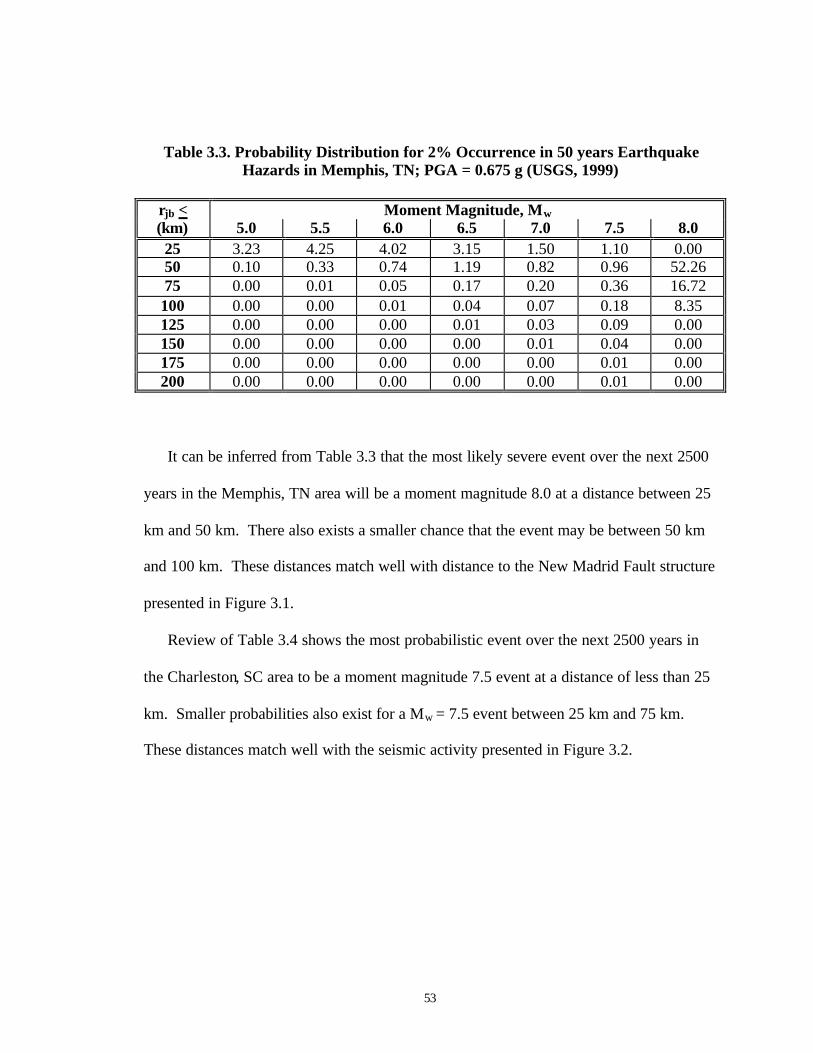
53
Table 3.3. Probability Distribution for 2% Occurrence in 50 years Earthquake Hazards in Memphis, TN; PGA = 0.675 g (USGS, 1999)
rjb < Moment Magnitude, Mw (km) 5.0 5.5 6.0 6.5 7.0 7.5 8.0 25 3.23 4.25 4.02 3.15 1.50 1.10 0.00 50 0.10 0.33 0.74 1.19 0.82 0.96 52.26 75 0.00 0.01 0.05 0.17 0.20 0.36 16.72 100 0.00 0.00 0.01 0.04 0.07 0.18 8.35 125 0.00 0.00 0.00 0.01 0.03 0.09 0.00 150 0.00 0.00 0.00 0.00 0.01 0.04 0.00 175 0.00 0.00 0.00 0.00 0.00 0.01 0.00 200 0.00 0.00 0.00 0.00 0.00 0.01 0.00
It can be inferred from Table 3.3 that the most likely severe event over the next 2500
years in the Memphis, TN area will be a moment magnitude 8.0 at a distance between 25
km and 50 km. There also exists a smaller chance that the event may be between 50 km
and 100 km. These distances match well with distance to the New Madrid Fault structure
presented in Figure 3.1.
Review of Table 3.4 shows the most probabilistic event over the next 2500 years in
the Charleston, SC area to be a moment magnitude 7.5 event at a distance of less than 25
km. Smaller probabilities also exist for a Mw = 7.5 event between 25 km and 75 km.
These distances match well with the seismic activity presented in Figure 3.2.

54
Table 3.4. Probability Distribution for 2% Occurrence in 50 years Earthquake Hazards in Charleston, SC; PGA = 0.758 g (USGS, 1999)
rjb < Moment Magnitude, Mw (km) 5.0 5.5 6.0 6.5 7.0 7.5 25 3.11 4.49 4.64 3.93 2.16 57.55 50 0.07 0.24 0.57 1.02 0.99 15.82 75 0.00 0.01 0.03 0.10 0.15 3.77 100 0.00 0.00 0.00 0.01 0.03 0.84 125 0.00 0.00 0.00 0.00 0.01 0.37 150 0.00 0.00 0.00 0.00 0.00 0.09 175 0.00 0.00 0.00 0.00 0.00 0.01 200 0.00 0.00 0.00 0.00 0.00 0.00
3.3 Mid-America Deep Soil Models
The lack of strong ground motion data (Mw > 5) in the central and eastern United
States causes difficulties when performing advanced analyses requiring input ground
motions. Research has been undertaken in association with the Mid-America Earthquake
(MAE) Center to develop synthetic ground motions to maintain consistency throughout
MAE Center projects. At the time of this study, the Herrmann & Akinci (1999) model
was considered to be the most appropriate. Model input data files are generated for use
with the Boore (1996) simulated ground motion program. Time series are generated
based on band limited white-noise stochastic simulations incorporated into random
vibration theory (Herrmann & Akinci, 1999). A concern with performance of white
noise ground motion models is that they do not accurately account for low frequency
surface waves. Additional duration from these long period waves may be critical for
earthquake analysis, as seen from field evidence presented in Youd (1999).
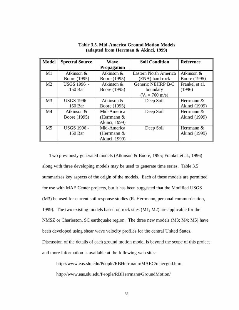
55
Table 3.5. Mid-America Ground Motion Models (adapted from Herrman & Akinci, 1999)
Model Spectral Source Wave
Propagation Soil Condition Reference
M1 Atkinson & Boore (1995)
Atkinson & Boore (1995)
Eastern North America (ENA) hard rock
Atkinson & Boore (1995)
M2 USGS 1996 - 150 Bar
Atkinson & Boore (1995)
Generic NEHRP B-C boundary
(Vs = 760 m/s)
Frankel et al. (1996)
M3 USGS 1996 - 150 Bar
Atkinson & Boore (1995)
Deep Soil Herrmann & Akinci (1999)
M4 Atkinson & Boore (1995)
Mid-America (Herrmann & Akinci, 1999)
Deep Soil Herrmann & Akinci (1999)
M5 USGS 1996 - 150 Bar
Mid-America (Herrmann & Akinci, 1999)
Deep Soil Herrmann & Akinci (1999)
Two previously generated models (Atkinson & Boore, 1995; Frankel et al., 1996)
along with three developing models may be used to generate time series. Table 3.5
summarizes key aspects of the origin of the models. Each of these models are permitted
for use with MAE Center projects, but it has been suggested that the Modified USGS
(M3) be used for current soil response studies (R. Herrmann, personal communication,
1999). The two existing models based on rock sites (M1; M2) are applicable for the
NMSZ or Charleston, SC earthquake region. The three new models (M3; M4; M5) have
been developed using shear wave velocity profiles for the central United States.
Discussion of the details of each ground motion model is beyond the scope of this project
and more information is available at the following web sites:
http://www.eas.slu.edu/People/RBHerrmann/MAEC/maecgnd.html
http://www.eas.slu.edu/People/RBHerrmann/GroundMotion/

56
http://www.eas.slu.edu/People/RBHerrmann/HAZMAP/hazmap.html
Input parameters necessary for the model will be discussed in the following paragraphs.
The main differences between current models (M1, M2) and the newly-proposed
ground motion models (M3, M4, M5) is the depth of the soil column and effects of that
overlying soil column on ground motions. Although linear aspects of the soil column are
considered in the proposed models (M3, M4, M5), the nonlinear nature of soil is not
taken into account. This will not be a concern for minor events, but high accelerations of
a severe event will likely induce strain levels that exceed the threshold strain, and soil
nonlinearity will be a concern during wave propagation. Studies by Idriss (1991) aft er
the Loma Prieta earthquake showed the influence of soft sites on resulting surface
accelerations. Figure 3.6 presents a summary of those results. Amplification of motions
Figure 3.6. Comparison of Acceleration at Soft Soil Sites to Rock Sites (Idriss, 1991)
57
is apparent at low accelerations, and damping may decrease surface accelerations during
a severe event. Application of these results to the Mississippi River Valley and Atlantic
Coastal Plain sediments still needs to be verified.
A stiffness profile for the NMSZ was generated by Herrmann et al. (1999) using
shallow shear wave velocities from previous studies. The stiffness of rock deposits was
estimated from Street (personal communication to Bob Herrmann, 1999). The generated
stiffness profile used in the Herrman and Akinci (1999) model is presented in Figure 3.5.
The stiffness profile, as well as the output of models M3, M4, and M5, is a function of
the depth of the soil column. A representation of the soil column depth was developed by
Herrmann et al. (1999) and is seen in Figure 3.7. This figure shows the overall extent of
thick sediments of the Mississippi River Valley, but does not provide the detail necessary
for an exact input depth at a specific location. For this study, a 600-m vertical column of
soil will be used in the Blytheville, AR and Steele, MO areas, and a 1000-m column of
soil over rock will be used in the Memphis, TN area (R. Herrmann, personal
communication, 1999). A linear soil- rock interface dipping relationship of 4 m per km
between Blytheville, AR and Memphis, TN, was based on information presented in
Figure 3.6, and will be assumed for model calculations. A generalized cross section of
the Mississippi River Valley is presented in Figure 3.8.
In Charleston, SC, there will be extensive deposits of Atlantic Coastal Plain soils
overlying a relatively insignificant thickness of Piedmont soils over bedrock. The
Clubhouse Crossing boring logs presented in Figure 3.10 (Gohn et al., 1983; Yantis et al,
1983) have been used to estimated a bedrock depth of 770 m and dipping rates of 2-

58
Figure 3.7. Soil Column Depth-Dependent Shear Wave Velocity (Vs) Profile used in Herrmann and Akinci (1999) Soil Models (M3,M4,M5)
(http://www.eas.slu.edu/People/RBHerrmann/HAZMAP/hazmap.html)
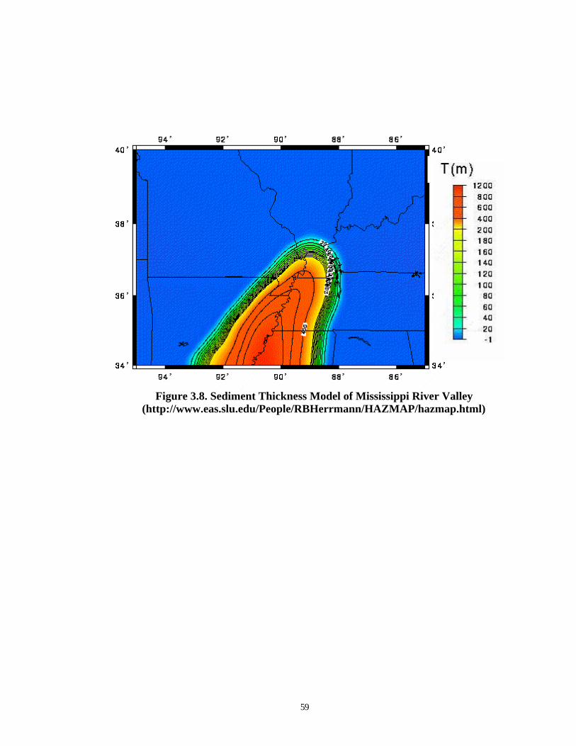
59
Figure 3.8. Sediment Thickness Model of Mississippi River Valley (http://www.eas.slu.edu/People/RBHerrmann/HAZMAP/hazmap.html)
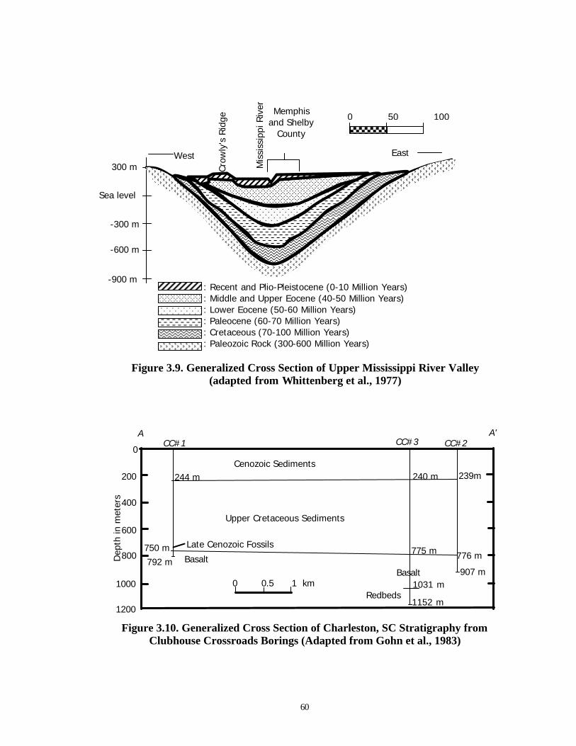
60
Figure 3.9. Generalized Cross Section of Upper Mississippi River Valley
(adapted from Whittenberg et al., 1977)
Figure 3.10. Generalized Cross Section of Charleston, SC Stratigraphy from Clubhouse Crossroads Borings (Adapted from Gohn et al., 1983)
0 0.5 1 km
Dep
th in
met
ers
A A' CC#1 CC#3 CC#2
244 m
750 m
792 m
Cenozoic Sediments
Upper Cretaceous Sediments
Late Cenozoic Fossils
Basalt 775 m
240 m
1031 m
1152 m Redbeds
Basalt 907 m
776 m
239m
0
200
400
600
800
1000
1200
Cro
wly
's R
idge
Mis
siss
ippi
Riv
er
Memphis and Shelby
County
West East
0 50 100
300 m
Sea level
-300 m
-600 m
-900 m : Recent and Plio-Pleistocene (0-10 Million Years) : Middle and Upper Eocene (40-50 Million Years) : Lower Eocene (50-60 Million Years) : Paleocene (60-70 Million Years) : Cretaceous (70-100 Million Years) : Paleozoic Rock (300-600 Million Years)

61
m/km for the Piedmont formation below the Atlantic Coastal Plain in the Charleston, SC
area. Using distances perpendicular to the Piedmont fall line, the Clubhouse Crossroads
logs were performed about 15 km from the epicenter of the 1886 earthquake, and about
35 km from Charleston. For analysis, a bedrock depth of 800 m will be used at the
epicenter, and the 2-m/km dipping rate will be used to produce a depth to bedrock of 840
m in Charleston.
A comparison of amax output by the five models for a magnitude 7.0 earthquake, is
presented in Figure 3.11. The USGS (M1; Frankel, 1996) model is the most
conservative. This model is based on rock sites (NEHRP B-C boundary) and does not
account for damping in the overlying soil column. The modified USGS model (M3)
accounts for damping through the depth of the soil column. This leads to lower
anticipated accelerations than the USGS model at close distances, but the models
converge at greater site distances (about 175 km). The Atkinson-Boore model (M2;
1995) is more conservative than the modified USGS (M3) at close distances. This model
becomes less conservative after about 30 km, and does not seem to account for lower
attenuation observed from events in the central and eastern United States. The two new
Mid-America deep soil models (M4 & M5) with mid-continent site effects lead to lower
accelerations than other models at close distances, and become more conservative at
greater distances (about 150 km). These models are still being calibrated and modified,
and may become more applicable after continued development.
Parametric studies show the differences in PGA responses obtained between an input
thickness of 600 m of soil and 1000 m of soil, in Figure 3.12. The depth of the soils

62
column appears most important at close distance, and the models tend to converge after
distances of about 100 km. When utilizing synthetic ground motions for liquefaction
analysis, the depth of soil column will be determined using bedrock depth and dipping
rates as presented above. Since the Herrmann & Akinci (1999) models were developed
primarily for use in the NMSZ, their reliability in the Charleston EQ region is not yet
verified.
Additional model input parameters for attenuation studies include moment
magnitude, hypocentral site distance, oscillatory damping, and range of periods. Moment
magnitude (Mw) can be varied between 3.0 and 8.5, and will be a function of the design
earthquake. Additional aspects of magnitude are contained Appendix II. The
hypocentral site distance can be varied from 1 km to 1000 km. This parameter will be a
combination of epicentral distance and hypocentral depth, as described in the previous
section. Oscillatory damping, c, is the critical damping of a single degree of freedom
system, and is typically considered to be five percent (0.05). The models (M3; M4; M5)
have three additional input parameters which can be used to control the primary range of
output frequencies.

63
Figure 3.11. Comparison of Accelerations Produced by Different Ground Motion
Models available for Mid-American Soils; Mw = 7.0
Figure 3.12. Effects of Soil Column Depth on PGA as Predicted by Herrmann &
Akinci (1999) Mid-America Deep Soil Model (M3); Mw = 7.0
0
0.5
1
1.5
2
1 10 100 1000
Joyner-Boore Distance (km)
PG
A (g
)
USGS (Frankel), 1996
Atkinson-Boore, 1995
Modified USGS, 1996(600 m soil)
Mid-America Deep Soil w/USGS-96 (600 m soil)
Mid-America Deep Soil w/AB-95 (600 m soil)
0
0.2
0.4
0.6
0.8
1
1.2
1.4
1 10 100 1000
Joyner-Boore Distance (km)
PG
A (g
)
Modified USGS, 1996 (600 m soil)
Modified USGS, 1996(800 m soil)
Modified USGS, 1996(1000 m soil)

64
3.4 Empirical Attenuation Relationships
To characterize an earthquake for geotechnical analysis, the peak horizontal
ground acceleration (PGA; amax) is required. Acceleration can be related to earthquake
magnitude and distance through attenuation relationships. A number of separate
empirical attenuation relationships for the eastern and central U.S. were reviewed in this
study. Attenuation relationships generated by the Herrmann & Akinci (1999) model
were previously discussed in Section 3.3 and displayed in Figures 3.11 and 3.12. These
relationships will be compared to current models and earlier attenuation curves.
Areas of primary concern in this study are within 50 km of fault zones. The
attenuation relationships will be carried out to 100 km to assess greater source-to-site
distances, and presented on a semi- log scale to show increased detail at close distances.
Since the analysis will be primarily compared to data produced from the Modified USGS
deep soil model (M3), results from this model will be included in each of the figures for
reference. Depths to bedrock and dipping relationships discussed in Section 3.2 will be
used when generating attenuation relationships from the Herrmann & Akinci (1999)
model. Hypocentral depths of 9.3 km and 10.7 km will be used for the NMSZ and
Charleston, SC earthquake regions respectively (Toro et al., 1997).
Proposed attenuation relationships for Mid-American soils at a moment
magnitude of 7.0 are presented in Figure 3.13. The Modified USGS (M3) model, that
will be used in this study, generally agrees with the previous relationships. Current
models (Herrmann & Akinci, 1999; Atkinson & Boore, 1997; Toro et al., 1997) predict
higher accelerations at short distances than previous studies (Nuttli & Herrmann, 1984),

65
due to the higher source scaling used. It has also been noticed that relationships based on
geotechnical investigations of historic liquefaction sites (e.g., Pond, 1996) generally
predict lower accelerations than rock models at close source distances and higher
accelerations at greater distance. This may be a result of increased damping due to the
nonlinear properties of the soils at close distances (high accelerations), and amplification
of soft sites at greater distances (low accelerations; as shown in Figure 3.6). Site specific
effects are not accounted for in most attenuation models, but likely control attenuation
relationships for specific geologic regions.
Figure 3.14 presents proposed attenuation relationships for Charleston, SC soils. For
comparison with previous studies, attenuation of a moment magnitude 6.0 and moment
magnitude 7.0 are reviewed. Field data from Martin (1990) is for moment magnitude 6.0
and moment magnitude 7.5, but the 1886 Charleston, SC earthquake on which the field
data were based is generally considered to be a moment magnitude 7.0 event. The Mw =
6.0 field data matches well with Mw = 6.0 attenuation relationships at close distances.
The Mw = 7.5 field data matches well with the Mw = 7.0 attenua tion relationship at
greater distances. This would support the hypothesis presented in the previous paragraph
that accelerations are damped at close distances (high accelerations) and amplified at
greater distance (low accelerations) at soft sites in Mid-America.
Figures 3.15 and 3.16 display magnitude effects on attenuation relations
determined from the Modified USGS deep soil model (M3; Herrmann & Akinci, 1999)
and Toro et al. (1997) rock motion model for sites in the NMSZ. Figures 3.17 and 3.18
display magnitude effects on attenuation relations using the same two models for the
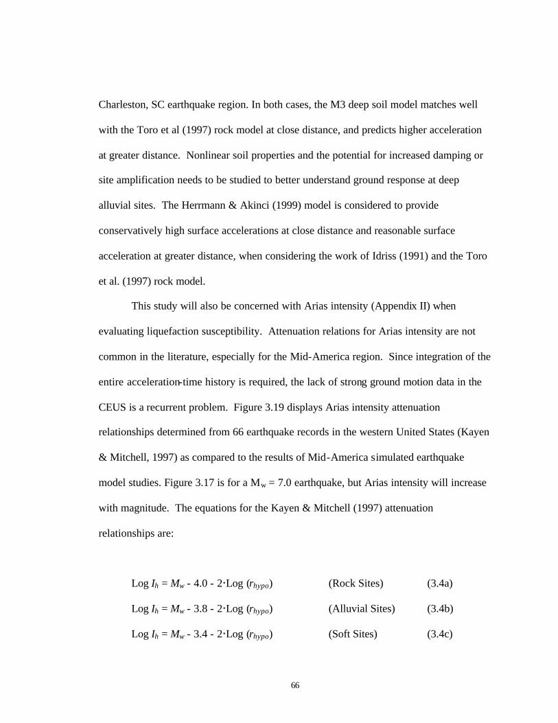
66
Charleston, SC earthquake region. In both cases, the M3 deep soil model matches well
with the Toro et al (1997) rock model at close distance, and predicts higher acceleration
at greater distance. Nonlinear soil properties and the potential for increased damping or
site amplification needs to be studied to better understand ground response at deep
alluvial sites. The Herrmann & Akinci (1999) model is considered to provide
conservatively high surface accelerations at close distance and reasonable surface
acceleration at greater distance, when considering the work of Idriss (1991) and the Toro
et al. (1997) rock model.
This study will also be concerned with Arias intensity (Appendix II) when
evaluating liquefaction susceptibility. Attenuation relations for Arias intensity are not
common in the literature, especially for the Mid-America region. Since integration of the
entire acceleration-time history is required, the lack of strong ground motion data in the
CEUS is a recurrent problem. Figure 3.19 displays Arias intensity attenuation
relationships determined from 66 earthquake records in the western United States (Kayen
& Mitchell, 1997) as compared to the results of Mid-America simulated earthquake
model studies. Figure 3.17 is for a Mw = 7.0 earthquake, but Arias intensity will increase
with magnitude. The equations for the Kayen & Mitchell (1997) attenuation
relationships are:
Log Ih = Mw - 4.0 - 2�Log (rhypo) (Rock Sites) (3.4a)
Log Ih = Mw - 3.8 - 2�Log (rhypo) (Alluvial Sites) (3.4b)
Log Ih = Mw - 3.4 - 2�Log (rhypo) (Soft Sites) (3.4c)

67
Figure 3.13. Comparison of Previously Proposed Attenuation Relationships for New Madrid Seismic Zone and Results of Modified USGS model (Mw = 7.0)
Figure 3.14. Comparison of Previously Proposed Attenuation Relationships for Charleston, SC EQ Region and Results of Modified USGS model (Mw = 7.0)
0.01
0.1
1
10
1 10 100Joyner-Boore Distance (km)
amax
(g)
Boore & Joyner, 1991Nuttli & Herrmann, 1984Pond, 1996 (Wabash Valley)Toro et al., 1997Atkinson & Boore, 1997Modified USGS, M3 (used here)
NMSZ
0.01
0.1
1
1 10 100
Joyner-Boore Distance (km)
amax
(g
)
Martin, 1990 (recommended Mw 6.0)
Martin 1990 (recommended Mw 7.5)
Modified USGS Mw = 6.0 (used here)
Modified USGS; Mw = 7.0 (used here)
Toro et al., 1997 (Mw = 6.0)
Toro et al., 1997 (Mw = 7.0)

68
Figure 3.15. Comparison of Toro et al. (lines; 1997) and Modified USGS (points) model for NMSZ on semi-log scale (5.5 < Mw < 8.0)
Figure 3.16. Comparison of Toro et al. (lines; 1997) Relationship and Modified USGS model (points) for NMSZ on log-log scale (5.5 < Mw < 8.0)
0
0.5
1
1.5
2
2.5
3
1 10 100
Joyner-Boore distance (km)
PG
A (g
)
Mw = 5.5
Mw = 6.0
Mw = 6.5
Mw = 7.0
Mw = 7.5
Mw = 8.0
0.01
0.1
1
10
1 10 100
Joyner-Boore distance (km)
PG
A (g
)
Mw = 5.5 Mw = 6.0
Mw = 6.5 Mw = 7.0
Mw = 7.5 Mw = 8.0

69
Figure 3.17. Comparison of Toro et al. (lines; 1997) and Modified USGS model (points) for Charleston, SC on semi-log scale (5.5 < Mw < 8.0)
Figure 3.18. Comparison of Toro et al. (lines; 1997) Relationship and Modified USGS model (points) for Charleston, SC on log-log scale (5.5 < Mw < 8.0)
0
0.5
1
1.5
2
2.5
3
1 10 100
Joyner-Boore distance (km)
PG
A (g
)
Mw = 5.5Mw = 6.0Mw = 6.5
Mw = 7.0Mw = 7.5
Mw = 8.0
0.01
0.1
1
10
1 10 100
Joyner-Boore distance (km)
PG
A (g
)
Mw = 5.5 Mw = 6.0
Mw = 6.5 Mw = 7.0
Mw = 7.5 Mw = 8.0

70
where Ih is the averaged Arias intensity in the x- and y-directions, and rhypo is the
hypocentral distance. Even though the Kayen & Mitchell relationships were determined
for California Sites, the Mid-America models match well at close Joyner-Boore
distances. At greater distance (rjb > 60 km), Arias intensity determined using the Mid-
America deep soil model (M3) tends to decrease at a lower rate than the model for
California sites. This will account for the lower attenuation rates observed in CEUS
soils. The effects of soil column thickness and soil conditions are shown in Figure 3.19.
The soil column thickness does not seem to have much effect, but potential for
amplification and damping at alluvial sites should not be ignored. The three M3 model
curves are more conservative than the Kayen & Mitchell (1997) relationship for alluvial
soils at distances less than 90 km.
Figure 3.20 displays attenuation relationships in the Charleston, SC earthquake
region, with the model studies providing an acceptable agreement with the Kayen &
Mitchell (1997) curves up to Joyner-Boore distances of 100 km. Since this study is
primarily concerned with earthquakes at close Joyner-Boore distance (rjb < 50 km), the
Kayen & Mitchell (1997) relationship sites will be considered acceptable. For Mid-
American sites at greater distances (rjb > 90 km), the specific Herrmann & Akinci (1999)
M3 model studies should be performed.
3.5 Summary
Distinct zones of seismic activity are apparent in microseismic records from the
New Madrid Seismic zone and Charleston, SC earthquake region. These areas are

71
Figure 3.19. Comparison of Previously Proposed Attenuation Relationships for New Madrid Seismic Zone and Results of Modified USGS model (Mw = 7.0)
Figure 3.20. Comparison of Previously Proposed Attenuation Relationships for New Madrid Seismic Zone and Results of Modified USGS model (Mw = 7.0)
0.1
1
10
100
1000
10000
1 10 100
Joyner-Boore Distance (km)
Ari
as In
tens
ity (c
m/s
)
Modified USGS 600 m soil
Modified USGS 800 m soil
Modified USGS 1000 m soil
Kayen, & Mitchell, 1997; Rock Sites
Kayen, & Mitchell, 1997; Alluvial Sites (used here)
Kayen, & Mitchell, 1997; Soft Sites
NMSZ
0.1
1
10
100
1000
10000
1 10 100
Joyner-Boore Distance (km)
Ari
as In
tens
ity (c
m/s
)
Modified USGS M3; Charleston, SC
Kayen, & Mitchell, 1997; Rock Sites
Kayen, & Mitchell, 1997; Alluvial Sites (used here)
Kayen, & Mitchell, 1997; Soft Sites
Charleston, SC

72
interpreted as areas near the fault structures in these geologic formations. While large
events have not occurred within the past 100 years, paleoseismic studies have shown a
recurrence interval on the order of 200 to 250 years for a significant (Mw > 7.0) event.
Depth and dipping rates of the soil column was estimated from model studies for the
NMSZ, and estimated from deep boring logs in the Charleston, SC earthquake region.
A ground motion model which accounts for linear effects of the deep soil column
in Mid-America is under development. Preliminary studies of this model have been
compared to existing empirical attenuation relationships for rock as well as soil. While
the model agrees well with data for small earthquakes (Mw < 5.0), it is expected that the
nonlinear soil effects induced by a severe event should cause vast differences between
soil and rock relationships. This may explain some of the differences between
attenuation relationships determined from engineering data associated with
paleoliquefaction studies, and models based on linear effects of the soil column calibrated
to low magnitude events and extrapolated to higher magnitude earthquakes.
Since the non- linear effects of the soil column are still being studied, acceleration
attenuation relationships generated by the modified USGS Mid-America deep soil model
(M3) were used in this study. This model is based on depth of soil column, hypocentral
distance, moment magnitude, and a generalized stiffness profile for the Mississippi River
Valley. Arias intensity relationships from the M3 model matched well with California
field performance data, and thus the Kayen & Mitchell (1997) attenuation relationship for
alluvial sites was also used in this study.

73
CHAPTER 4
LIQUEFACTION RESPONSE OF SOILS
4.1 Overview
A number of methodologies are available for evaluating the cyclic response of soils.
Liquefaction analyses performed in this study can be categorized under the:
§ Cyclic stress approach (e.g., Seed & Idriss, 1971);
§ Cyclic strain approach (e.g., Dobry et al., 1982);
§ Arias intensity approach (e.g., Kayen & Mitchell, 1997).
The concepts of critical void ratio (e.g., Casagrande, 1936; Appendix I) and a critical
state line for sands (e.g., Been, 1999; Appendix I) will be applied when evaluating these
methods.
Cyclic-stress and cyclic-strain based methods were originally derived from laboratory
tests performed to evaluate soil behavioral response to earthquake shaking. The cyclic
response of soils is controlled by factors such as soil fabric, pre-straining, stress history,
and aging effects (Seed, 1979) that cannot be replicated in the laboratory. Due to the
difficulty and expense associated with obtaining undisturbed field samples of sandy and
silty soils, empirical relations from in-situ test parameters are commonly compared to
field performance of soil deposits which have been subjected to historic earthquakes.
The Arias intensity approach for liquefaction evaluation has developed utilizing field
performance databases as well as recorded earthquake seismograms. Since this method

74
utilizes the entire earthquake acceleration-time history, the uncertainties of simplified
procedures and empirical magnitude scaling factors (MSF) can be minimized.
4.2 Cyclic Stress Approach
The cyclic stress approach is the most commonly used procedure in practice to
estimate liquefaction resistance of sandy soils. To represent earthquake ground motions
with a single parameter, a simplified procedure was developed by Seed & Idriss (1971).
Liquefaction resistance is evaluated by comparison of a soil index property to the cyclic
stress ratio (CSR). The CSR is the average cyclic shear stress in a layer (τavg) normalized
to the effective overburden stress (σ'vo). It is a function of earthquake duration
(magnitude), maximum surface acceleration (amax), depth to soil element being analyzed
(z), and total (σvo) and effective (σ'vo) vertical stress. The maximum surface acceleration
(amax) can be determined from acceleration time histories or estimated from attenuation
relationships (Fig. 3.13; Fig. 3.15; Toro et al., 1997). For a moment magnitude Mw = 7.5
earthquake, the CSR is generally presented as:
dvo
vo
vo
avg rg
aCSR ⋅
⋅
⋅≈=
'65.0
'max
σσ
σ
τ (4.1)
where rd is a stress reduction factor with depth, and other variables are described above.

75
4.2.1 Stress Reduction Coefficient
Stress reduction factors, rd, were initially presented in Seed & Idriss (1971) for sites
with sand in the upper 15-meters, and may be approximated (Robertson & Wride, 1997):
rd = 1.0 - 0.00765 z when z < 9.15 m (4.2a)
rd = 1.174 - 0.0267 z when 9.15 < z < 23 m (4.2b)
rd = 0.744 - 0.008 z when 23 < z < 30 m (4.2c)
rd = 0.5 when z > 30 m (4.2d)
where z is depth in meters. Re-evaluation of improved data sets and interpretation led to
the following expressions (Idriss, 1999):
( ) ( )[ ]wd Mzzr ⋅+= βαexp (4.3a)
with
( ) ( )[ ]133.573.11sin126.101.1 +⋅−−= zzα (4.3b)
( ) ( )[ ]142.528.11sin118.0106.0 +⋅+= zzβ (4.3c)
where z is depth in meters and < 25 m. Figure 4.1 compares the initial average
relationship to revised relationships as well as expected uncertainty from preliminary
field studies. The Idriss (1999) stress reduc tion factors will be used for this study.

76
Figure 4.1. Stress reduction Coefficients for Simplified Procedures
0
5
10
15
20
25
30
35
0 0.2 0.4 0.6 0.8 1Stress Reduction Coefficient, rd
Dep
th (m
)
Idriss, 1999
Seed & Idriss, 1971
Mw = 5.5 6.5 7.5 8
Range of values for different soil profiles (Seed & Idriss, 1971)
77
4.2.2 Magnitude Scaling Factors
The moment magnitude of an earthquake will influence duration of shaking, and thus
increase the number of significant stress cycles. With an increased number of significant
stress cycles at the same stress ratio, the soil will exhibit a lower resistance to
liquefaction. The effects of earthquake magnitude are not included in the cyclic stress
ratio equation, Eq 4.1, so magnitude scaling factors (MSF) were developed. The
reference magnitude for cyclic stress based analysis is 7.5.
Initially MSF trends were developed from a combination of field and laboratory data,
based on relationships between magnitude and number of equivalent stress cycles. A
relationship between moment magnitude, Mw, and significant stress cycles, neq, can be
expressed as (Seed et al., 1985):
94.40007.0 weq Mn ⋅≈ (4.4)
A number of studies concerning variation in magnitude scaling factors have been
performed using combinations of theory and field data (Ambraseys, 1988; Arango, 1996;
Andrus & Stokoe, 1997), with results and NCEER recommendations presented in Youd
& Noble (1997).
Re-evaluation of field data sets and laboratory tests on frozen samples led to a revised
magnitude scaling factor (Idriss, 1999):
MSF = 31.9 (Mw)-1.72 (4.5)

78
Figure 4.2. Effect of Revised Stress Reduction Coefficients on Magnitude Scaling Factors
(Idriss, 1999 factors used in this study)
0
0.5
1
1.5
2
2.5
3
3.5
4 5 6 7 8 9
Earthquake Magnitude, M w
Mag
nit
ud
e S
calin
g F
acto
r (M
SF
)
Idriss (1999) Seed et al. (1985)
Ambraseys (1988) Arango (1996)
Arango (1996) Andrus & Stokoe (1997)
z = 24 mz = 16 mz = 8 mz = 0 m

79
These studies also determined that the depth of liquefied layers affects the magnitude
scaling factors through the stress reduction coefficient, rd. Equation 4.3 displays the
magnitude dependent stress reduction coefficient. Figure 4.2 presents the range of
magnitude scaling factors determined from various studies. The magnitude scaling
factors recommended by the NCEER (1997) workshop were between the lower bound of
the Arango (1996) curves and the Andrus & Stokoe (1997) curve. The Idriss (1999)
factors match well with the NCEER recommendations for depths between 8 and 16 m,
and will be used in this study for simplified cyclic stress based analysis.
4.2.3 Cyclic Resistance Ratio
The CSR is a function of the earthquake motions, while the cyclic resistance ratio
(CRR) represents the liquefaction resistance of the deposit. Databases from post-
earthquake field investigations have been utilized to generate demarcation curves relating
a stress normalized resistance parameter of an in-situ test [e.g., (N1)60, Vs1, qc1; Section
2.3.2] to the soils resistance to cyclic loading from a magnitude 7.5 earthquake (CRR7.5).
Field performance data from earthquakes at magnitudes other than 7.5 are corrected to
equivalent CSR7.5 values as:
MSFCSR
CSR =5.7 (4.6)

80
Figure 4.3. Key Aspects of Simplified Cyclic Stress based Charts
Field data are separated into sites that have or have not displayed surface manifestations
of liquefaction behavior. A demarcation line, known as the CRR7.5, is generated between
the liquefaction and non- liquefaction sites. This line was originally estimated by hand,
but mathematical representations are generally preferred for spreadsheet application.
Figure 4.3 displays an example field case history data base, and notes key features of a
typical chart.
Cyclic stress-based analysis consists of the following steps:
1. Determine amax and Mw for design earthquake;
2. Determine the profile of cyclic stress ratio (CSR) with depth using equations 4.1 and
4.3 or a site specific analysis (e.g., SHAKE91; Idriss & Sun, 1992);
Mw = 7.5
0.0
0.1
0.2
0.3
0.4
0.5
0.6
0 10 20 30 40 50
Overburden Stess Normalized In-Situ Test Resistance Parameter
Cyc
lic R
esis
tanc
e R
atio
7.5
(CR
R)
LiquefactionevidenceNo liquefactionevidence
Liquefaction Likely
Liquefaction Not Likely
Fines Content Dependent
Cyclic Resistance
Ratio
Increasing Fines Content /
Decreasing CRR
Chart valid for Mw = 7.5

81
3. Evaluate critical layer resistance parameters from SPT, CPT, or Vs profiles;
4. Estimate fines content from laboratory index tests or field correlations;
5. Determine cyclic resistance ratio from charts or simplified formulas as a function of
in-situ test resistance parameter and fines content;
6. Calculate a factor of safety (FS) against liquefaction for the design earthquake as
(Youd & Noble, 1997):
MSFCSR
CRRFS ⋅
= 5.7 (4.7)
where MSF is a magnitude scaling factor equal to one for earthquakes with moment
magnitude (Mw) of 7.5.
4.2.4 Application to Paleoliquefaction Studies
For paleoliquefaction studies and backcalculation of accelerations, the calculated FS
will be close to unity in cases of marginal liquefaction, and below unity for extensive
liquefaction. Questions arise concerning the validity of using of post-earthquake field
data to estimate pre-earthquake in-situ state, and thus backcalculation of prehistoric
accelerations. The use of field performance data in liquefaction studies became popular
because sampling destroyed structure and aging effects, which are known to increase
liquefaction resistance. At a location of surface evidence of liquefaction, such as sand
boils and lateral spreads, it would be expected that the post-earthquake soil conditions
would be extremely disturbed with a loss of structure and aging effects.
82
It has been shown that sites that liquefy during an earthquake event will likely liquefy
in subsequent events (Youd, 1984; Yasuda & Tohno, 1988). This process has been
termed re- liquefaction. Earthquakes have been occurring throughout the evolution of the
planet, so at liquefaction sites in seismically-active regions it would be expected that soils
have undergone more than one liquefaction event over the history of the deposit.
Younger sand dikes erupting through older sand dikes have been noticed in the NMSZ,
but are not common. These previous events would destroy the natural alluvial deposition
structure, and replace it with a loose pluvial structure resembling that of water
sedimentation (Pond, 1996). With time, the soil structure and aging effects would form
in a similar manner as they had before the previous liquefaction event. It has been shown
that strength increase in sands from aging is a log- linear process (logarithm for time, and
linear for strength increase; Seed, 1979). A majority of the strength increase occurs
within the first 100 years after deposition, and then the effects level off. If sites with pre-
earthquake field data are not available, it would be desirable to test the properties of the
soil after a time period where aging would better resemble the pre-earthquake structure.
4.2.5 Liquefaction Evaluation from Standard Penetration (SPT) Test Data
Seed et al. (1983) developed a field performance database for liquefaction analysis
using uncorrected standard penetration test (SPT) N-value. This study was comprised of
sites where surface manifestations of liquefaction (e.g. sand boils, lateral spreading, etc.)
were either evident or not evident during post-earthquake field reconnaissance
investigations. SPT values were plotted against the CSR7.5 (Eq. 4.1; Eq. 4.6) from the
earthquake event, and a demarcation line (CRR7.5) was determined from the boundary

83
between sites where liquefaction was evident and other sites where no surface evidence
of liquefaction was observed. Some data were also classified as "marginal evidence," and
these points were expected to lie closer to the cyclic resistance ratio curve.
Since this database was generated from different studies throughout the world, the
variation in N-value from SPT procedures was recognized to influence the position of the
CRR curve (Seed et al., 1985). Current simplified curves using SPT data are compared to
the (N1)60 value, which has been corrected to an energy efficiency of 60 percent for
procedural variation, and normalized to an overburden stress of 1-atmosphere (Chapter
2). Additional case histories have been used to slightly modify the position of the CRR,
but due to the variability in the SPT, additional analyses should be performed on
borderline cases to reduce the inherent uncertainty. An empirical equation for the cyclic
resistance ratio adapted by NCEER (1997) is:
432
32
5.7 1 hxfxdxbxgxexcxa
CRR++++
+++= (4.8)
where the parameter x = (N1)60cs, and the empirical constants consist of: a = 4.844�E-2,
b = -1.248�E-1, c = -4.721�E-3, d = 9.578�E-3, e = 6.136E-4, f = -3.285E-4, g= -1.673E-
5, and h = 3.714E-6. The parameter (N1)60cs is the stress normalized SPT blowcount
corrected for energy efficiency and fines content. The fines content correction can be
estimated by (Robertson & Wride, 1997):

84
( ) ( )601601 NKN scs ⋅= (4.9a)
−⋅
+= )5(
3075.0
1 FCK s (4.9b)
Figure 4.3 displays the Seed et al. (1985) SPT database along with the NCEER (1997)
curves. Four charts are presented: (a) clean sand data with fines content (FC) less than 5
percent; (b) silty sand data with fines content between 5 and 15 percent; (c) sandy silt
data with fines content between 15 and 35 percent; and (d) silt data with fines content
greater than 35 percent.
The SPT case history data and the mathematical representation of the cyclic
resistance ratio curves match well. For clean sands, there is sufficient data that suggests a
relatively linear relationship between CRR and N-value for low N-value soils, which
trends towards a vertical asymptote at about 30 blows per foot. The silty sand (FC=15%)
curve matches well with the case histories, but there are insufficient data to support a
vertical asymptote. The data for sandy silt (FC between 15 and 35%) match well with the
proposed trends, but there are insufficient data to support a vertical asymptote. The data
for the silty soils (FC > 35%) match well with the proposed trends. While there is only 1-
point at a high cyclic stress ratio (0.6), this point supports the concept of a vertical
asymptote at an N-value of about 17.

85
Figure 4.4. SPT Liquefaction Site Database and NCEER CRR curves (a) FC (%) < 5; (b) 5 < FC (%) < 15; (c) 15 < FC (%) < 35; (d) FC (%) > 35
(adapted from Seed et al., 1986; Robertson & Wride, 1997)
a. Clean Sand b. Silty Sand
c. Sandy Silt d. Silt
0.0
0.1
0.2
0.3
0.4
0.5
0.6
0 10 20 30 40 50
(N1)60
Cyc
lic R
esis
tan
ce R
atio
(C
RR
) FC (%) < 5
0.0
0.1
0.2
0.3
0.4
0.5
0.6
0 10 20 30 40 50
(N1)60
Cyc
lic R
esis
tan
ce R
atio
(C
RR
) FC (%) = 15
0.0
0.1
0.2
0.3
0.4
0.5
0.6
0.7
0 10 20 30 40 50
(N1)60
Cyc
lic R
esis
tan
ce R
atio
(CR
R)
FC (%) = 35 15
0.0
0.1
0.2
0.3
0.4
0.5
0.6
0.7
0 10 20 30 40 50
(N1)60
Cyc
lic R
esis
tan
ce R
atio
(CR
R)
FC (%) = 35

86
It can be expected that CRR trends for various levels of fines content will be similar.
The concept of a limiting vertical asymptote makes sense when considering the existence
of a critical void ratio (Casagrande, 1936) and a critical state line for sands (Been, 1999).
More detail on the critical state parameters for sands is presented in Appendix I. The
currently recommended curves by NCEER (1997) have good agreement with the field
data as well as concepts relating to the shear behavior of sands.
4.2.6 Liquefaction Evaluation from Cone Penetration Test (CPT) Data
Since the CPT is more reliable than the SPT, a simplified cyclic-stress based
procedure using the cone penetration test was formed. When the CPT method was
initially developed, there were only a limited number of case histories with available cone
tip resistance data. Therefore, correlations between SPT N-value and CPT tip resistance
were used along with the SPT liquefaction case history database presented in the previous
section (Robertson & Campanella, 1985; Seed & DeAlba, 1986). To reduce uncertainty
from the SPT-CPT correlation, a CPT only database was developed by Shibata &
Teparaksa (1988). New field data have been added by Stark & Olson (1995) and Olson
& Stark (1998). The CPT database now contains 172 independent case histories of
seismic sites where surface evidence of liquefaction has or has not been evident.
With the cone penetration test, a soil specimen is not retrieved, resulting in questions
as to the soil type and fines content. Many different classification schemes are currently
available for cone testing based on tip resistance and friction ratio, FR, or tip resistance
and pore pressure parameter, Bq. These schemes are discussed in detail in Section 2.3.3.
In addition to tip resistance data, it is necessary to estimate fines content in sandy layers.

87
Correlations between fines content and Friction Ratio (FR = fs/qt�100) have been
presented in Suzuki et al. (1995a; 1995b), Robertson & Wride (1997), as well as Olsen
(1997). In contrast, and a lack of correlation between Friction Ratio and fines content has
been shown in Arango (1997). Confirmation of CPT fines content correlations by
sampling and index testing is recommended (Mitchell & Brandon, 1998). In clean sands,
the penetration pore water pressures will be close to hydrostatic. The pore pressure
reading behind the tip will also be useful in estimating water table depth as well as soil
strata demarcations.
The cyclic resistance ratio for CPT qc has been represented as a numerical
approximation by Robertson & Wride (1997; 1998) and Olsen (1997). The NCEER
(1997) workshop participants reviewed these methods and recommend the following
expression from Robertson & Wride (1997):
if 50 < (qc1N)cs < 160 ( )
08.01000
933
15.7 +
⋅= csNcq
CRR (4.10a)
if (qc1N)cs < 50 ( )
05.01000
83.0 15.7 +
= csNcq
CRR (4.10b)
where (qc1N)cs is the stress-normalized cone tip resistance corrected for apparent fines
content. Appropriate normalization factors for this method were presented earlier in
Table 2.4. The concept of a clean sand corrected tip resistance has not been

88
recommended by the NCEER (1996) committee, but it is based on a similar concept as
presented for the SPT where:
(qc1N)cs = Kc�qc1N (4.11)
with methods to estimate Kc based on grain characteristics as presented in Robertson &
Wride (1997; 1998). Figure 4.5 displays the Olson & Stark (1998) database along with
the NCEER (1997) cyclic resistance ratio curves. Four charts are presented: (a) clean
sand data; (b) silty sand data; (c) sandy silt data; (d) all 3 NCEER curves. The CRR
curves for 15 percent and 35 percent fines content were calculated using the Kc clean
sand correction factor. The cone tip resistance presented in Olsen & Stark (1998) was
normalized using the Kayen et al (1992) method, with the resulting units presented in
megapascals (MPa). The CRR calculated from the Robertson & Wride (1997) formula
was converted to MPa as:
atm
MPaqq ccq
⋅⋅=
1013.01 (4.12)
where qc1 is the Kayen et al. (1992) normalized tip resistance, and qc1N in the Robertson
& Wride (1997; 1998) normalized tip resistance.
The proposed curves and field performance match well for the CPT data, but the
Robertson & Wride (1997; 1998) curve appears to be slightly unconservative for all soil
types. There are no CPT field data supporting a vertical asymptote for any of the soil

89
Figure 4.5. CPT Liquefaction Database and NCEER Recommended CRR (a) Clean Sand; (b) Silty Sand; (c) Sandy Silt; (d) NCEER Curves (Adapted from Olson & Stark, 1998; Robertson & Wride, 1997)
a. Clean Sand b. Silty Sand
d. NCEER Curvesc. Sandy Silt
0
0.1
0.2
0.3
0.4
0.5
0.6
0 5 10 15 20 25 30qc1 (MPa)
Cyc
lic R
esis
tan
ce R
atio
(C
RR
)
M=7.5
Clean Sand0.25 < D50 (mm) < 2.0Apparent FC < 5 %
0
0.1
0.2
0.3
0.4
0.5
0.6
0 5 10 15 20 25 30qc1 (MPa)
Cyc
lic R
esis
tan
ce R
atio
(C
RR
)M=7.5
Silty Sand0.10 < D50 (mm) < 0.25Apparent FC = 15 %
0
0.1
0.2
0.3
0.4
0.5
0.6
0 5 10 15 20 25 30qc1 (MPa)
Cyc
lic R
esis
tan
ce R
atio
(C
RR
)
M=7.5
Silty Sand-Sandy SiltD50 (mm) < 0.10Apparent FC = 35 %
0
0.1
0.2
0.3
0.4
0.5
0.6
0 5 10 15 20 25 30qc1 (MPa)
Cyc
lic R
esis
tan
ce R
atio
(C
RR
)
M=7.5
Silty Sand-Sandy SiltD50 (mm) < 0.10Apparent FC = 35 %
Silty Sand0.10 < D50 (mm) < 0.25
Apparent FC = 15 %
Clean Sand0.25 < D50 (mm) < 2.0
Apparent FC < 5 %

90
types. While the Robertson & Wride (1997; 1998) curve is recommended up to a CSR of
0.5, additional data from sites that have not liquefied at high CSR values would lead to
more confidence in the suggested CRR curve.
4.2.7 Liquefaction Evaluation from Shear Wave Velocity (Vs) Data
Cyclic stress-based procedures were based on the premise that liquefaction resistance
is governed by relative density. Since in-situ penetration test resistance parameters are
also strongly influenced by relative density, a correlation between in-situ test parameters
and liquefaction resistance should exist. The work of Dobry et al (1982) determined that
seismically- induced shear strains are more important than seismically- induced stresses in
the liquefaction response of soils. To adapt the cyclic strain-based procedures to the
well-known simplified cyclic stress based methods, shear stress is related to shear strain
using the shear modulus. Since the shear modulus is directly related to shear wave
velocity through the fundamental equa tion G = ρVs2, a theoretical basis exists for the
development of cyclic resistance ratio curves using shear wave velocity data. Andrus &
Stokoe (1997) present the derivation of a shear wave velocity dependent CRR for
relatively small strains (e.g., less than about 5 x 10⁻¹ %). For higher strain levels, a
limiting value of shear wave velocity is expected to be approached. Shear wave velocity
is strongly influenced by void ratio and the coordination number of the soil fabric (e.g.,
Robertson et al., 1995; Santamarina et al., 1999). Therefore, the concepts of critical void
ratio (Casagrande, 1936) and a unique critical state line for sands (Been, 1999) can be
incorporated into the derivation of this CRR equation.

91
As in the case of the SPT, and CPT, a database of field case histories has been
developed comparing shear wave velocity at seismically-active sites that have or have not
shown surface manifestations of liquefaction. The database contains over 75 sites subject
to 25 earthquakes between 1906 and 1995 (Andrus et al., 1999). Most of the shear wave
velocity data is from post earthquake field investigations, so the soil fabric is likely
disturbed from its pre-earthquake sate. This may increase shear wave velocity from
additional cyclic pre-straining, or reduce shear wave velocity if aging and cementation
affects were destroyed by excessive cyclic straining. Since the same shear wave velocity
measurements at a site were used for multiple earthquakes, additional scatter is expected
when comparing the database results to theoretical curves.
The cyclic resistance ratio for overburden stress normalized shear wave velocity (Vs1)
has been represented as a numerical approximation by Andrus & Stokoe (1997) and
updated by Andrus et al. (1999):
−
−⋅+
⋅=
*11
*1
21
5.711
100sss
s
VVVb
VaCRR (4.13)
where Vs1=Vs / (σvo’)n and is the stress normalized shear wave velocity using a stress
exponent n = 0.25 and σvo’ is in atmospheres (Robertson et al., 1992b), Vs1* is the
limiting upper value of Vs1 for liquefaction occurrence, and a and b are curve fitting
parameters equal to 0.022 and 2.8 respectively. The limiting value of shear wave
velocity in sandy soils has been estimated to be:

92
Figure 4.6. Vs Liquefaction Site Database and Recommended CRR Curves (a) Clean Sand; (b) Silty Sand; (c) Sandy Silt; (d) Andrus et al. (1999) Curves
(adapted from Andrus & Stokoe, 1997; Andrus et al., 1999)
a. Clean Sand b. Silty Sand
c. Sandy Silt d. Curves
0.0
0.1
0.2
0.3
0.4
0.5
0.6
0 100 200 300 400
Vs1
Cyc
lic R
esis
tan
ce R
atio
FC (%) < 5
0.0
0.1
0.2
0.3
0.4
0.5
0.6
0 100 200 300 400Vs1
Cyc
lic R
esis
tan
ce R
atio
FC (%) = 15
0.0
0.1
0.2
0.3
0.4
0.5
0.6
0 100 200 300 400Vs1
Cyc
lic R
esis
tan
ce R
atio
FC (%) = 35
0.0
0.1
0.2
0.3
0.4
0.5
0.6
0 100 200 300 400Vs1
Cyc
lic R
esis
tan
ce R
atio
FC (%) = 35 15 < 5

93
Vs1* = 215 m/s FC (%) < 5 (4.14a)
Vs1* = 215 - 0.5�(FC-5) m/s 5 < FC (%) < 35 (4.14b)
Vs1* = 200 m/s FC (%) > 35 (4.14c)
Figure 4.6 displays the Andrus & Stokoe (1997) database along with the Andrus et al.
(1999) cyclic resistance ratio curves. Four charts are presented: (a) clean sand data; (b)
silty sand data; (c) sandy silt data; (d) all 3 NCEER curves. The data agree well with the
proposed CRR curves, but the Andrus et al. (1999) curve appears to be slightly
unconservative for all soil types. There are limited Vs field data supporting a vertical
asymptote for any of the soil types, so additional data from sites that have not liquefied at
high CSR values would lead to greater confidence in the CRR curves.
4.2.8 Extrapolation to High CSR
It is anticipated that an extreme event in Mid-America could result in cyclic stress
ratios on the order of 1.0 or higher at close epicentral distances (Toro et al., 1997).
Current field performance data are is limited to CSR values typically below 0.4, with
most data in the 0.1 to 0.2 range. Laboratory tests on reconstituted specimens can not
fully replicate soil fabric, which contributes significantly to liquefaction resistance.
Advances in sampling of granular soils by freezing techniques allows in-situ soil fabric to
remain relatively undisturbed prior to laboratory testing. Therefore, the cyclic resistance
of a deposit may be more accurately determined from laboratory testing.

94
Figure 4.7. Comparison of CRR curves and Laboratory Frozen Specimens Figure 4.8. Comparison of Vs1 CRR curve and Laboratory Frozen Specimens
0
0.1
0.2
0.3
0.4
0.5
0.6
0.7
0.8
0.9
1
0 100 200 300 400
qt1N
Cyc
lic S
tres
s R
atio
, σd/2
σo'
6 Japanese sitesFrozen samples
(Suzuki et al., 1995)
FC < 10
Cyclic Triaxial to5% Double
Amplitude Strain
15 cycles
0
0.1
0.2
0.3
0.4
0.5
0.6
0.7
0.8
0.9
1
0 50 100 150 200 250
Vs1
Cyc
lic S
tres
s R
atio
, σd/2
σo'
6 Japanese sitesFrozen samples(Suzuki et al., 1995)
Cyclic Trixial to5% Double Amplitude Strain
15 cycles
Robertson & Wride, 1997
Equation 4.15

95
Field performance based CRR curves can be validated by comparison of laboratory
based cyclic resistance from frozen specimens to in-situ test parameters taken adjacent to
the sample location. A study by Suzuki et al (1995b) presents field shear wave velocity
and cone tip resistance data as compared to laboratory cyclic resistance from frozen
specimens. Figures 4.7 and 4.8 display the data compared to qc1 and Vs1 respectively.
The Robertson & Wride (1997; 1998) curves match the average value of the data
presented in Suzuki et al. (1995) study, but a number of points are misclassified. The
uncertainty inherent when using simplified curves should result in a conservative
estimate of liquefaction resistance, such as the Seed et al. (1985) SPT-type CRR curves.
The Robertson & Wride (1997; 1998) curves do not approach an asymptotic value at high
values of CSR. Considering the concepts of a critical void ratio and critical state for
sands, an asymptotic value is expected for CRR curves.
The work of Andrus & Stokoe (1997) and Andrus et al. (1999) present an equation
for the CRR based on shear wave velocity data. The format of this equation leads to an
asymptotic value of shear wave velocity at high values of CSR. A similar form will be
adapted for the CRR determined from CPT qc1N data:
( )NcNc
Nc
qqbq
aCRR1
*1
1
350 −+
⋅= (4.15)
where a and b are curve fitting parameters equal to 0.7 and 9.33 respectively. The
Andrus & Stokoe (1997) term *1sV
b− (or in this case *1Ncq
b− ) is left out of the

96
equation since it is accepted that the CRR does not pass through the origin (NCEER,
1997). The limiting value of normalized cone tip resistance in clean sands has been
estimated to be 230 from cyclic triaxial test data. To validate this curve for field
performance data, Figure 4.8 compares Equation 4.15 and the Robertson & Wride (1997;
1998) CRR equation (Eq. 4.10) for the Olson & Stark (1998) CPT field performance
database. Equation 4.15 is more conservative than currently-recommended methods, but
seems to better fit all of the field data. It incorporates critical state concepts for sands
with a limiting value of normalized CPT tip resistance.
Figure 4.9. Comparison of CRR curves with CPT Field Performance data
0
0.1
0.2
0.3
0.4
0.5
0.6
0 5 10 15 20 25 30qc1 (MPa)
Cyc
lic R
esis
tan
ce R
atio
(C
RR
)
M=7.5
Clean Sand0.25 < D50 (mm) < 2.0Apparent FC < 5 %
Equation 4.15
Robertson & Wride,
1997

97
4.3 Cyclic Strain Approach
The cyclic strain approach was developed by Dobry et al. (1982) as a more rational
means to accommodate that the liquefaction resistance of soils is controlled not only by
relative density, but also by soil fabric, level of prestraining, lateral stress coefficient
(Ko), overconsolidation ratio (OCR), and aging effects. Strain-controlled cyclic triaxial
tests to evaluate porewater pressure generation due to cyclic straining are apparently not
affected by relative density, fabric effects, prestraining, and aging, as seen in Figure 4.10
(Dobry et al., 1982). The soil stiffness (G) increases with increased relative density, and
decreased in void ratio (Hardin and Drnevich, 1972). This will in turn reduce shear-
induced strains, and increase liquefaction resistance. The generality of the cyclic strain
approach is appreciated further because cyclic generation of porewater pressures has been
shown to be dependent on lateral stress and OCR (Vasquez-Herrera et al., 1988), but
relatively independent of the sand tested (Ladd et al., 1989).
The cyclic strain method consists of the following steps (Dobry et al., 1982):
1. Determine strain level (γc) with depth;
2. Compare induced-strain level to the plastic threshold strain level (γtp = 10-2 %);
3. Evaluate porewater pressure buildup using normalized curves;
4. Decide if the pore pressures in the soil will cause initial liquefaction (u = σvo).

98
Figure 4.10. Density Independence of Initial Porewater Pressure Generation During Cyclic Strain Controlled Tests on Some Sand (after Ladd et al., 1989)
Figure 4.11. Sand Type and Preparation Method Independence of Porewater Pressure Generation in Cyclic Strain Controlled Tests (after Ladd et al., 1989)
0
0.01
0.02
0.03
0.04
0.05
0.06
0.001 0.01 0.1
Cyclic Shear Strain (%), γc
r u =
∆u
/ σ
' 3
Dr = 45Dr = 60Dr = 80
0
0.2
0.4
0.6
0.8
1
0.001 0.01 0.1 1
Cyclic Shear Strain, γ c (%)
Po
re P
ress
ure
Rat
io,
u r /
' 3
Crystal Silica Sand, dry vibrationCrystal Silica Sand, wet roddingCrystal Silica Sand, dry vibrationSand No. 1, moist tampingSand No. 1, moist tampingMonterey No. 0, moist tamping
n = 10 cycles Dr = 60 %

99
4.3.1 Shear Strain Level with Depth
The strain level with depth can be estimated by using two primary methods:
1. Simplified procedures developed by Seed & Idriss (1971) can be modified using
maximum shear modulus (Go = Gmax) and normalized G/Gmax degradation schemes;
2. Site-specific analysis, such as SHAKE91 (Idriss & Sun, 1992).
This study will only be concerned with modified simplified procedures. The equations
necessary for the simplified analys is utilize the definition of shear modulus (Eq. 4.16) to
modify the simplified CSR equation (Eq. 4.1):
Gτ
γ = (4.16)
( ) dvo rGGGg
a
γ
σγ
maxmax
max65.0 ⋅= (4.17)
where γ is strain level, τ is the earthquake induced stress level, G is the strain level
dependent shear modulus, amax is the maximum horizontal surface acceleration, g is the
acceleration due to gravity, σvo is the total vertical stress, rd is the stress reduction
coefficient presented in Equation 4.3, Gmax is the maximum small strain shear modulus,
and (G/Gmax)γ is the modulus reduction factor at the appropriate strain level. The
effective vertical stress (σvo') cancels out of this equation, since it is on both sides of
Equation 4.1. The maximum small strain shear modulus, Gmax, can be directly obtained
from the shear wave velocity determined from SCPTu soundings as:
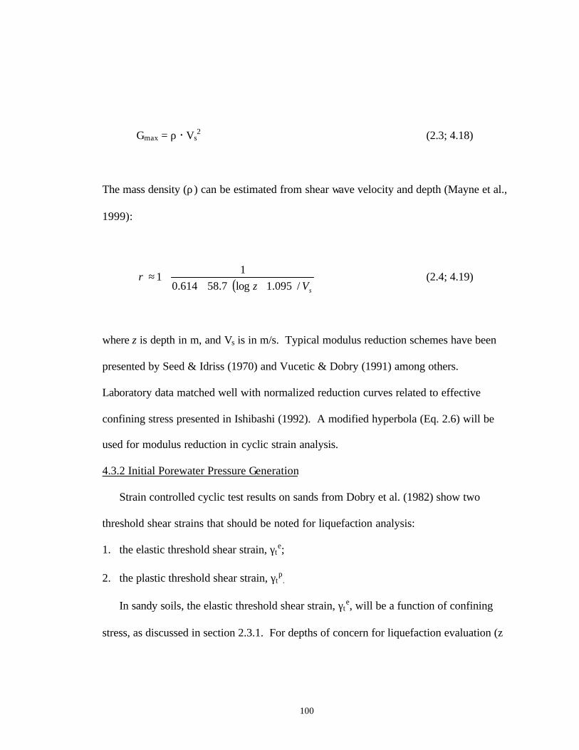
100
Gmax = ρ � Vs2 (2.3; 4.18)
The mass density (ρ) can be estimated from shear wave velocity and depth (Mayne et al.,
1999):
( ) sVz /095.1log7.58614.0
11
+⋅++≈ρ (2.4; 4.19)
where z is depth in m, and Vs is in m/s. Typical modulus reduction schemes have been
presented by Seed & Idriss (1970) and Vucetic & Dobry (1991) among others.
Laboratory data matched well with normalized reduction curves related to effective
confining stress presented in Ishibashi (1992). A modified hyperbola (Eq. 2.6) will be
used for modulus reduction in cyclic strain analysis.
4.3.2 Initial Porewater Pressure Generation
Strain controlled cyclic test results on sands from Dobry et al. (1982) show two
threshold shear strains that should be noted for liquefaction analysis:
1. the elastic threshold shear strain, γte;
2. the plastic threshold shear strain, γtp
.
In sandy soils, the elastic threshold shear strain, γte, will be a function of confining
stress, as discussed in section 2.3.1. For depths of concern for liquefaction evaluation (z

101
< 20 m), the overburden stresses should be within the 0.5- to 2-atmosphere range. This
will result in an elastic threshold strain on the order of 1x10⁻³ percent.
Once the plastic threshold shear strain (γtp) is exceeded, pore pressures will be
induced by undrained cyclic loading. Figures 4.7 and 4.8 display the independence of
plastic threshold strain with regards to sand type, preparation method (fabric), and
relative density. The plastic threshold shear strain in sands is considered to be equal to
1x10⁻² percent (Dobry et al., 1982).
If the plastic threshold shear strain is not reached, cyclic pore pressures will not be
induced and liquefaction will not occur. The reduced shear modulus at γtp will be
approximately equal to 0.8�Gmax. Therefore the following screening equation can be
generated from Equations 4.17:
dvo rGg
a⋅
⋅⋅=
max
max
23.1σ
γ (4.20)
where all terms are as defined above. If γ induced by the earthquake is less than 1x10⁻²
(γtp), liquefaction will not occur.
4.3.3 Cyclic Pore Pressures from Normalized Curves
For induced strain levels higher than the plastic threshold shear strain (γtp), an
evaluation of cyclic pore pressure generation will be desired. Vasquez-Herrera et al.
(1988) developed an empirical method relating the stress state of the soil to the shape of
the pore pressure generation curve. This method was developed for flow liquefaction of

102
embankments, but will be adapted for use with cyclic liquefaction. The key soil and
empirical parameters used in the development of this method are:
• soil liquefaction will occur at a critical pore pressure ratio (ru = ∆u/σvo’);
• a threshold pore pressure (rut) may exist below initial liquefaction (ru = 1);
• rut is a function of Kc and α 'up;
• Kc is the ratio of vertical stresses to horizontal stresses (σ1c' / σ3c');
• α 'up is a flow liquefaction failure surface where loss of contact points between soil
grains will leads to structural collapse, rapid increase in pore pressure, and flow to a
critical void ratio (Alarcon-Guzman et al., 1988);
• the number of cycles to liquefaction is a function of rut, γtp, induced cyclic strains
(γcy), and the empirical coefficients α and β;
• The empirical curve fitting parameter α = 4.78 - 1.91�Kc;
• The empirical curve fitting parameter β = 2.96 - 0.78 � Kc;
The normalized pore pressure generation curves will be adapted for free field level
ground cyclic liquefaction by using the following:
• the threshold pore pressure generation coefficient (rut) will be equal to one (Seed,
1979);
• the in-situ coefficient of lateral stress, Ko = σho' / σvo', will be equivalent to 1 / Kc;
• the flow surface will not contribute to level ground liquefaction.
For evaluation of pore pressure generation, the in-situ coefficient of lateral stress (Ko)
will need to be estimated. Analysis procedures for determining in-situ state was shown in

103
Chapter 2, and recommended correlations will be presented here. To estimate the lateral
stress coefficient from CPT data in clean sands, Ko-OCR-φ' relationships presented in
Mayne & Kulhawy (1982) will be utilized:
Ko = (1-sinφ')� OCRsinφ' (4.21)
The friction angle (φ') can be estimated from cone tip resistance (qt) data as (Kulhawy &
Mayne, 1990):
φ' = 17.6o + 11�log(qt�(pa/σvo')0.5) (4.22)
where pa is atmospheric pressure and σvo' is the effective overburden stress. The
estimation of Ko in clean unaged quartz sands is obtained with Equations 4.21 and 4.22 in
an iterative solution using the following expression based on calibration chamber test
data (Mayne, 1995):
27.0
31.022.0'
192.0 OCRPP
qK
a
vo
a
to ⋅
=
−σ
(4.23)
Three additional equations will be used to estimate the shape of pore pressure generation
curves. The number of cycles to failure (nt) can be represented as:

104
( ) ( )utp
tc
utt
r
rn
−⋅−=
2β
γγα (4.24)
where rut is the threshold pore pressure ratio equal to one, and the other terms are as
defined previously. The number of cycles generated by a seismic event will be a function
of the earthquake magnitude, as discussed in section 4.2.2 on magnitude scaling factors:
94.40007.0 weq Mn ⋅≈ (4.4)
Therefore, the pore pressure ratio (ru = ∆u/σ3') for level ground earthquakes as a function
of strain cycles can be expressed as:
8
68.018.21
02.1
⋅+
⋅+
=t
eq
t
eq
t
eq
u n
n
n
nn
n
r (4.25)
with all parameters as defined above. If ru equals unity for an earthquake of n cycles,
initial liquefaction will occur. Figure 4.12 displays the shape of porewater pressure
generation curves set by φ’ as a function of the ratio of number of cycles to number of
cycles to failure.

105
Figure 4.12. Normalized Pore Pressure Generation Curves as a Function of Ko (adapted from Vasquez-Herrera et al., 1989)
0
0.2
0.4
0.6
0.8
1
0 0.2 0.4 0.6 0.8 1
neq/nt
r u =
∆u
/ σh'
Increasing OCR
K0 = 1.0
K = 0.45
K0 = 0.5
K0 = 0.6
K0 = 0.8

106
4.4 Arias Intensity Method
A developing method for liquefaction analysis based on Arias intensity of earthquake
records has the advantage that it does not require magnitude scaling factors. Although
this method seems promising, lack of strong motion data in the Mid-America Earthquake
region area leads to increased reliance on ground motion models. Arias intensity
represents the cumulative energy per unit weight in a given direction that is absorbed by a
set of single degree of freedom oscillators (Arias, 1970). Arias intensity (Ih) can be
calculated as the sum of Arias Intensity in the x- (Ixx) and y- (Iyy) directions as (Kayen &
Mitchell, 1997):
( ) ( )dttag
dttag
IIIoo t
y
t
xyyxxh ∫∫ +=+=0
2
0
2
22ππ
(4.26)
where g is the acceleration due to gravity, ax(t) is the horizontal acceleration time history
in one direction, and ay(t) is the horizontal acceleration time history in the direction
perpendicular to ax(t). The numerical integration of acceleration time histories to
determine intensity should be performed on corrected acceleration time histories using
trapezoidal integration (Youd et al., 1997).
Similarly to the CSR from the Seed & Idriss (1971) simplified procedure, the Arias
intensity will typically decrease with depth. Depending upon the depth where the time
history was recorded and the depth of the liquefied layer, it may be necessary to apply a
depth correction factor, rb:

107
Ihb = Ih � rb (4.26)
The Arias intensity depth correction factor was primarily determined from analysis of
synthetic seismograms propagated through soil profiles using the SHAKE 1-D equivalent
linear program. Significant scatter existed within the data (as is also evident in the rd
correction factor for the simplified cyclic stress procedure), with average values as:
rb = 1.0 - 0.07z when z < 6 m (4.27a)
rb = 0.76 - 0.03z when 6 m < z < 10 m (4.27b)
rb = 0.46 when z > 10 m (4.27c)
where z is in meters. Field data from the Superstition Hills and Elmore Ranch
(California) earthquakes of 1987 lie between the averages presented above and one
standard deviation below the averages (Kayen & Mitchell, 1997).
Simplified liquefaction resistance curves have been generated comparing Arias
Intensity (Ihb) to penetration resistance [(N1)60 and qc1] for field case histories where
strong ground motion data have been readily available (Kayen & Mitchell, 1997). These
curves are based on limited field data from California (n=28), and thus Arias Intensity
Resistance to liquefaction curves (IhbR) are considered quite approximate. Considering
Arias intensity field performance data for the CPT, cyc lic stress-based field data for the
CPT, stress-based laboratory tests on frozen specimens compared to CPT tip resistance,

108
Figure 4.13. Arias intensity Liquefaction Field Data compared to curves from Kayen & Mitchell (1997) and Equation 4.28
0
1
10
100
0 10 20 30 40qc1 (MPa)
I hb (
m/s
)
No Liq, FC <5% Liquefaction, FC < 5%
Liquefaction, FC < 15% No Liq, FC > 30%
Liquefaction, FC > 30%
LiquefactionNot Likely
LiquefactionLikely
D50 < 0.15 mmFC > 30%
D5 0 > 0.25 mmFC < 5%
{ Kayen & Mitchell, 1997
Equation 4.28
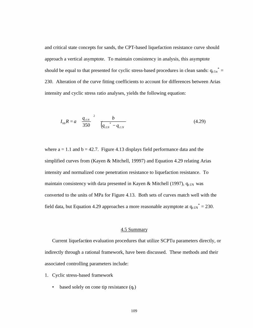
109
and critical state concepts for sands, the CPT-based liquefaction resistance curve should
approach a vertical asymptote. To maintain consistency in analysis, this asymptote
should be equal to that presented for cyclic stress-based procedures in clean sands: qc1n* =
230. Alteration of the curve fitting coefficients to account for differences between Arias
intensity and cyclic stress ratio analyses, yields the following equation:
( )NcNc
Nchb qq
bqaRI
1*
1
21
350 −+
⋅= (4.29)
where a = 1.1 and b = 42.7. Figure 4.13 displays field performance data and the
simplified curves from (Kayen & Mitchell, 19997) and Equation 4.29 relating Arias
intensity and normalized cone penetration resistance to liquefaction resistance. To
maintain consistency with data presented in Kayen & Mitchell (1997), qc1N was
converted to the units of MPa for Figure 4.13. Both sets of curves match well with the
field data, but Equation 4.29 approaches a more reasonable asymptote at qc1N* = 230.
4.5 Summary
Current liquefaction evaluation procedures that utilize SCPTu parameters directly, or
indirectly through a rational framework, have been discussed. These methods and their
associated controlling parameters include:
1. Cyclic stress-based framework
• based solely on cone tip resistance (qt)

110
• base solely on shear wave velocity (Vs)
2. Arias intensity based framework
• based solely on cone tip resistance (qt)
3. Cyclic strain based method
• based on engineering parameters (Ko, OCR, φ’, Dr) determined from shear wave
velocity (Vs) and cone tip resistance (qt)
Anticipated cyclic stress ratio (CSR = τ / σvo’) and Arias intensity (Ihb) from a severe
event in Mid-America are anticipated to be much higher than current curves have been
validated in China, Japan, and California. Utilization of the concepts of critical state for
sands in association with data from cyclic tests on frozen specimens has been used to
determine cyclic resistance ratio curves that progress to an asymptotic value. These
curves have been validated as a conservative lower bound for clean sand field data from
liquefaction sites. The same curve format with altered empirical coefficients (a & b) has
been applied to Arias intensity based field data. These proposed curves are more
internally consistent, and encompass the available liquefaction case data. This provides a
conservative curve for simplified analysis.

111
CHAPTER 5 GEOTECHNICAL SITE CHARACTERIZATION OF SOILS IN MID-AMERICA
5.1 Overview
Proper classification and characterization of soils are necessary for a reliable
liquefaction analysis. Soil behavior type classification methods based on CPT test results
have been discussed previously, and verification through laboratory index testing is
desirable. This chapter will present results from field and lab tests on soils in Mid-
America. Simple laboratory index tests were performed on surface samples obtained
from select sites. Field testing by seismic piezocone tests (SCPTu) are utilized to
determine stratigraphic layering and stiffness profiles with depth at 12 test sites located in
the New Madrid seismic zone and Charleston, SC earthquake region. These sites are
generally associated with seismic events, and most have shown surface evidence of
liquefaction.
5.2 Laboratory Index Testing
Grain characteristics of sands have been shown to influence soil susceptibility to
liquefaction (e.g., Yamamuro et al., 1999) as well as steady state characteristics (e.g.,
Poulos et al., 1985). A study of index properties associated with granular soils of Mid-
America was undertaken as part of this research. A limited series of laboratory index
testing of soils from the Memphis, TN area and Blytheville, AR has been conducted at

112
Georgia Tech. Soil index properties from liquefaction sites in the Charleston, SC area
(Cullen, 1985) and the Shelby Forest site (Liu et al., 1997) are also reviewed. The
parameters studied and associated laboratory tests are:
♦ Grain Size Distribution (Sieve Analysis - ASTM D422);
♦ Fines Content (Percent finer than U.S. No. 200 Sieve - ASTM D422);
♦ Limiting Void Ratios (emax - ASTM D4254: emin - ASTM D4253);
♦ Specific Gravity, (Gs - ASTM D854);
♦ Roundness (Visual inspection of magnified particles).
Figure 5.1 shows characteristic values of roundness (R) and associated particle shapes
(Youd, 1973). Well-rounded particles are often associated with aged, water-borne
sediment. Very angular (R<0.15) particles are characteristic of freshly crushed
aggregates from rock quarries. Figures 5.2 through 5.5 display images of sands from
Shelby County, TN, and Blytheville, AR captured using a microscope and digital image
analysis software. These images will be used for visual determination of roundness
characteristics. Figure 5.6 displays grain size distributions for Mid-America sands
determined from laboratory testing. Table 5.1 presents grain characteristics of sands
from this study (Memphis, TN & Blytheville, AR), West Memphis AR (personal
communication Marshall, 1998), Shelby Forest TN (Liu et al., 1997), and Charleston SC
(Cullen, 1985). In addition, indices from standard reference sands (Been et al., 1987;
Mayne & Kulhawy, 1991) are presented in this table for comparison.
Index properties from four primary Mid-America depositional geologies are
presented:

113
• Mississippi River Valley - WRMS, Memphis TN; B-1, West Memphis AR; Yarbro
Excavation, Blytheville AR;
• Loess Bluffs - Shelby Forest, north Memphis TN;
• Wolf River - Shelby Farms and Houston Levee, east Memphis TN;
• Atlantic Coastal Plain - North-South and East-West trenches, Charleston SC;
Grab samples were taken at shallow surface depths from exposed layers, in most cases.
Sands from West Memphis, AR and Shelby Forest, TN were sampled at depth using SPT
methods. The tested soils are uniformly graded, relatively clean (low fines content) fine
quartz sands. The sands from Mississippi River Valley were finer than the Wolf River
sands. The Atlantic Coastal plain sediments were of similar median grain size to the
Mississippi Valley deposits, but were more uniform with no fines. Each of the soils
analyzed in this study were subangular from visual classification. Drawings of particles
presented in Cullen (1985) appeared to be more angular than the magnified pictures
presented in Figures 5.2 to 5.6.

114
Figure 5.1. Characteristic Values of Roundness (adapted from Youd, 1973)
R < 0.17 R ≈ 0.20 R ≈ 0.30
R ≈ 0.35 R ≈ 0.50 R ≈ 0.70
Very Angular Angular Subangular
Subrounded Rounded Well-Rounded

115
Figure 5.2. Magnified View of Particles from Shelby Farms (SF)
1 mm

116
Figure 5.3. Magnified View of Particles from Houston Levee (HL)
1 mm

117
Figure 5.4. Magnified View of Particles from Wolf River at Mississippi River (WRMS)
1 mm

118
Figure 5.5. Magnified View of Particles from Yarbro Excavation (YE)
1 mm

119
Figure 5.6. Grain Size Curves for Mid-America Sands
0
10
20
30
40
50
60
70
80
90
100
0.010.1110
Grain Size (mm)
Per
cen
t F
iner
by
Wei
gh
t
Shelby FarmsHouston LeveeWRMSYarbro ExcavationW. Memphis (2 m)W. Memphis (4.5 m)North-South TrenchEast-West Trench
Fines (Silt and Clay) Fine Sand Medium Sand
Coarse Sand
Gravel

Table 5.1. Grain Characteristics for Sands from Mid-America and Standard Reference Sands Sand D50
(µm) D10 (µm)
Uniformity Coefficient
Percent Fines
Specific Gravity
Roundness Description emax emin
Shelby Farms (Memphis, TN)
530 310 2.0 0 2.66 ≈ 0.30 Subangular 0.76 0.53
Houston Levee (Memphis, TN)
600 400 1.6 0 2.66 ≈ 0.30 Subangular 0.80 0.57
WRMS (Memphis, TN)
190 90 2.3 5-7 2.64 ≈ 0.30 Subangular 0.88 0.59
Yarbro Ex. (Blytheville, AR)
410 210 2.3 1 2.62 ≈ 0.30 Subangular 0.79 0.51
B-1 @ 2 m (W. Memphis, AR)
180 80 2.5 6.7 NA NA NA NA NA
B-1 @ 4.5 m (W. Memphis, AR)
210 140 1.7 2.7 NA NA NA NA NA
Shelby Forest (Shelby Co., TN)4
NA NA NA NA 2.62 NA NA 0.88 0.47
North-South Trench (Charleston, SC)1
200 140 1.3 0 2.66 ≈ 0.25 Subangular 0.91 0.62
East-West Trench (Charleston, SC)1
150 95 1.8 0 2.67 ≈ 0.25 Subangular 0.96 0.67
Ticino2 (Italy)
530 360 1.6 0 2.67 0.38 Subrounded 0.89 0.60
Toyoura3 (Japan)
160 130 1.46 - 2.64 - Subangular 0.98 0.61
Ottawa2 (United States)
530 350 1.7 0 2.66 0.55 Rounded 0.79 0.49
Monterey No. 02
(United States) 370 250 1.6 0 2.65 0.35 Subrounded 0.82 0.54
1 Cullen, 1985 2 Been et al., 1987 3 Mayne & Kulhawy, 1991 4 Liu et al., 1997

121
5.3 Seismic Piezocone Test Results
Field-testing for this study concentrated on a total of 12 sites, with six sites located in
the New Madrid seismic zone, four sites in Memphis, TN, and two sites in Charleston,
SC. One or more SCPTu sounding was performed at each site. A majority of the sites
and sounding locations selected were in coordination with the work of previous
paleoliquefaction studies (Tuttle et al., 1998; Tuttle et al., 1996; Wolf et al., 1998;
Collier, 1998; Van Arsdale, 1998a; Schweig, 1998; Martin, 1990). Most of the sites have
shown evidence of prior liquefaction, such as sand blows, feeder dikes, lateral spreads,
settlement, subsidence, or cracks. This study is meant to complement paleoliquefaction
investigations and evaluate deeper source soils and site effects. Site maps, photos, and
descriptions are available in Appendix IV.
Figure 5.7 displays the main areas of testing for this study. The test sites are broken
up into three different sections:
• Shelby County, TN area: Representing test sites in Memphis and surrounding areas
associated with a Joyner-Boore distance of approximately 50-km and 1000-m
thickness of sediments over bedrock. Epicentral distances from the New Madrid
1811 event ranged from 40- to 90-km, and were greater than 100-km for other
historic events.
• Northeast Arkansas and Southeast Missouri: Representing test sites in Blytheville
AR, Steele MO, and Caruthersville MO areas with a Joyner-Boore distance of less
than 15 km and 600-m thickness of sediments overlying bedrock. Epicentral
distances ranged from 40- to 65-km for events in 1811 to 1812.

122
Figure 5.7. Test areas presented on USGS 1996 2% PE in 50 year Central and Eastern U.S. Hazard Map;
Memphis ; NE AR / SE MO ; Charleston, SC . (http://www.geohazards. cr.usgs.gov/eq/hazmaps/250pga.gif)

123
• Charleston, SC area: Representing test sites in the Charleston SC area with a Joyner-
Boore distance of about 25 km to the center of the city and 820-m thickness of
sediments overlying bedrock. Epicentral distances ranged between 5- and 10-km for
the earthquake of 1886.
5.3.1 SCPTu Profiles
Table 5.2 displays the list of seismic piezocone test soundings that are analyzed,
along with pertinent site and sounding information. Unless noted, longitude and latitude
measurements were recorded with a Garmin hand-held unit with an accuracy of about +
0.001 degrees (15 m). Figure 5.8 displays a legend used for the soil profiles generated
from SCPTu data using methods discussed in Chapter 2. Figures 5.9 through 5.23
display soundings that will be discussed for liquefaction analysis of Mid-American soils.
Additional seismic cone profiles generated by this study, with termination depths greater
than 10-m are contained in Appendix V.
Sand
Silt
Clay
Silty Sand
Sandy Silt
Clayey Silt
Silty Clay
Figure 5.8. General soil classification legend for profiles depicted

124
Table 5.2. Seismic Piezocone Testing in Mid-America Earthquake Region Location Type of
Test2,3,4 Sounding
I.D. Longitude
North (degrees)
Latitude 5
East (degrees)
Max Test
Depth (m)
Shelby County, TN Area Shelby Farms (SF) 10T SCPTu2 MEMPH-G 35.1172 -89.8055 31.40 SF Shooting Range 10T SCPTu2 SFSR-01 35.1292 -89.8416 30.40 Houston Levee (HL) 10T SCPTu2 MEMPH-H 35.1083 -89.7305 20.40
Shelby Forrest 10T SCPTu2 SFOR-01 35.3578 -90.0188 21.40
Northeast Arkansas and Southeast Missouri Area Yarbro Excavation 10T SCPTu2 YARB-01 35.9823 -89.9331 28.00
Bugg 40 10T SCPTu2 BUGG-01 35.9728 -89.9078 38.50 Bugg 40 10T SCPTu2 BUGG-02 35.9723 -89.9079 34.20 3MS617 15T SCPTu2 3MS617-A 35.9926 -89.8356 32.50
Huey House 15T SCPTu2 HUEY-01 35.9835 -89.8865 26.00 Dodd Farm 15T SCPTu2 DODD-01 36.0949 -89.8483 30.85 Dodd Farm 15T SCPTu2 DODD-02 36.0946 -89.8483 25.35 Dodd Farm 15T CPTu2 DODD-03 36.0942 -89.8482 32.30
Johnson Farm 15T SCPTu2 JOHN-01 36.1192 -89.8439 25.15
Charleston, SC Hollywood Ditch1 SCPTu2 HW-4 32.739 -80.240 19.20
Thompson Industrial1 SCPTu2 TIS-01 32.919 -80.047 14.4 1 Longitude and latitude determined from street address using http://www.mapblast.com 2 10 T refers to a load cell with a maximum capacity of 10 tons 3 15T refers to a load cell with a maximum capacity of 15 tons 4 u2 refers to penetration pore pressure measurements taken behind the tip 5 negative values of latitude refer to west

Figure 5.9. Seismic Piezocone Test Results from Shelby Farms, TN (MEMPH-G)
SEISMIC CONE PENETROMETER DATA SCHOOL OF CIVIL AND ENVIRONMENTAL ENGINEERINGSOUNDING PERFORMED FOR MAEC GEORGIA INSTITUTE OF TECHNOLOGY
Date: 9/16/98 Truck: GT GeoStar Predrill: - Cone Type: Hogentogler 10 TonTest Site: Shelby Farms Test No: MEMPH-G GWT: 6 m Filter: Type 2Location: Memphis, TN Operators: James Schneider
Distance to Sounding Axis from Seismic Source: 1 m Tracy Hendren
Clay
Sand
0
5
10
15
20
25
30
35
0 15 30 45qt (MPa)
Dep
th B
GS
(m
)
0
5
10
15
20
25
30
35
0 1 2 3 4 5 6 7 8
Friction Ratio (%)
0
5
10
15
20
25
30
35
-500 1000 2500
u2 (kPa)
0
5
10
15
20
25
30
35
0 250 500
Vs (m/sec)
Clay
Sand
Sandy Silt

Figure 5.10. Seismic Cone Test Results from Shelby Farms Shooting range, TN (SFSR-01)
SEISMIC CONE PENETROMETER DATA SCHOOL OF CIVIL AND ENVIRONMENTAL ENGINEERINGSOUNDING PERFORMED FOR MAEC GEORGIA INSTITUTE OF TECHNOLOGY
Date: 3/22/99 Truck: GT GeoStar Predrill: - Cone Type: Hogentogler 10 TonTest Site: Shelby Farms Shooting RangeTest No: SFSR-01 GWT: 2 m Filter: Type 2Location: Shelby County, TN N: 35
o07.750 W: 089
o50.493+ 30.1' Operators: James Schneider
Distance to Sounding Axis from Seismic Source: 1.0 m Tom Casey
0
5
10
15
20
25
30
35
0 10 20 30 40qt (MPa)
Dep
th B
GS
(m)
0
5
10
15
20
25
30
35
0 1 2 3 4 5 6 7 8Friction Ratio (%)
0
5
10
15
20
25
30
35
-100 200 500u2 (kPa)
Possible Poor Filter
Saturation
0
5
10
15
20
25
30
35
0 250 500Vs (m/sec)
Sand
Sand
Sandw. Silt Lenses
Sandy Clay to Clay

Figure 5.11. Seismic Piezocone Test Results from Houston Levee, TN (MEMPH-H)
SEISMIC CONE PENETROMETER DATA SCHOOL OF CIVIL AND ENVIRONMENTAL ENGINEERINGSOUNDING PERFORMED FOR MAEC GEORGIA INSTITUTE OF TECHNOLOGY
Date: 9/17/98 Truck: GT GeoStar Predrill: - Cone Type: Hogentogler 10 TonTest Site: Houston Levee Test No: MEMPH-H GWT: 5 m Filter: Type 2Location: Germantown, TN Distance to Sounding Axis from Seismic Source: 1 m Operators: James Schneider
Tracy Hendren
0
5
10
15
20
25
0 5 10 15 20 25qt (MPa)
Dep
th B
GS
(m
)
0
5
10
15
20
25
0 1 2 3 4 5 6 7 8Friction Ratio (%)
0
5
10
15
20
25
-500 500 1500 2500u2 (kPa)
0
5
10
15
20
25
0 250 500Vs (m/sec)
SMSilt
Sand
Stiff Clay
Clayey Silt
Sand

Figure 5.12. Seismic Piezocone Test Results from Shelby Forrest, TN (SFOR-01)
SEISMIC CONE PENETROMETER DATA SCHOOL OF CIVIL AND ENVIRONMENTAL ENGINEERINGSOUNDING PERFORMED FOR MAEC GEORGIA INSTITUTE OF TECHNOLOGY
Date: 3/23/99 Truck: GT GeoStar Predrill: - Cone Type: Hogentogler 10 TonTest Site: Shelby County, TN Test No: SFOR-01 GWT: 6 m Filter: Type 2Location: Shelby Forrest N: 35o21.468 W: 090o01.130 + 36.5' Operators: James Schneider
Distance to Sounding Axis from Seismic Source: 1 m Tom Casey
0
5
10
15
20
25
0 10 20 30 40 50qc (MPa)
Dep
th B
GS
(m
)
0
5
10
15
20
25
0 1 2 3 4 5 6 7 8Friction Ratio (%)
0
5
10
15
20
25
-500 500 1500 2500u2 (kPa)
0
5
10
15
20
25
0 200 400 600Vs (m/sec)
This Study
Liu et al., 1997
Clayey Silt
V. Dense Sand
Dens
Clay
Silty Sand

Figure 5.13. Seismic Piezocone Test Results from Yarbro Excavation, AR (YARB-01)
SEISMIC CONE PENETROMETER DATA SCHOOL OF CIVIL AND ENVIRONMENTAL ENGINEERINGSOUNDING PERFORMED FOR MAEC GEORGIA INSTITUTE OF TECHNOLOGY
Date: 10/21/98 Truck: GT GeoStar Predrill: - Cone Type: Hogentogler 10 TonTest Site: Yarbro Excavation Test No: YARB-01 GWT: 4 m Filter: Type 2Location: Blytheville, AR N: 35o58.940' W: 089o55.986 + 12 m Operators: James Schneider
Distance to Sounding Axis from Seismic Source: 0.75 m Ken Thomas
0
5
10
15
20
25
30
35
0 10 20 30 40qt (MPa)
Dep
th B
GS
(m)
0
5
10
15
20
25
30
35
0 1 2 3 4 5 6 7 8Friction Ratio (%)
0
5
10
15
20
25
30
35
-100 200 500u2 (kPa)
0
5
10
15
20
25
30
35
0 250 500Vs (m/sec)
Sand
Sand
Sand
Sand
Sand

Figure 5.14. Seismic Piezocone Test Results from Bugg 40, AR (BUGG-01)
SEISMIC CONE PENETROMETER DATA SCHOOL OF CIVIL AND ENVIRONMENTAL ENGINEERINGSOUNDING PERFORMED FOR MAEC GEORGIA INSTITUTE OF TECHNOLOGY
Date: 10/21/98 Truck: GT GeoStar Predrill: - Cone Type: Hogentogler 10 TonTest Site: Bugg 40 Test No: BUGG-01 GWT: 4 m Filter: Type 2Location: Blytheville, AR N: 35
o58.366 W: 089
o54.468 + 9 m Operators: James Schneider
Distance to Sounding Axis from Seismic Source: 0.75 m Ken Thomas
0
5
10
15
20
25
30
35
40
0 15 30 45qt (MPa)
Dep
th B
GS
(m)
0
5
10
15
20
25
30
35
40
0 1 2 3 4 5 6 7 8Friction Ratio (%)
0
5
10
15
20
25
30
35
40
-500 500 1500 2500
u2 (kPa)
0
5
10
15
20
25
30
35
40
0 250 500Vs (m/sec)
CleanSand
Clayey Silt
Stiff Clay
Sand

Figure 5.15. Seismic Piezocone Test Results from Bugg 40, AR (BUGG-02)
SEISMIC CONE PENETROMETER DATA SCHOOL OF CIVIL AND ENVIRONMENTAL ENGINEERINGSOUNDING PERFORMED FOR MAEC GEORGIA INSTITUTE OF TECHNOLOGY
Date: 10/24/98 Truck: GT GeoStar Predrill: - Cone Type: Hogentogler 10 TonTest Site: Bugg 40 Test No: BUGG-02 GWT: 4 m Filter: Type 2Location: Blytheville, AR N: 35o58.335' W: 089o54.475' + 9 m Operators: James Schneider
Distance to Sounding Axis from Seismic Source: 0.75 m Ken Thomas
0
5
10
15
20
25
30
35
0 15 30 45
qt (MPa)
Dep
th B
GS
(m)
0
5
10
15
20
25
30
35
0 1 2 3 4 5 6 7 8
Friction Ratio (%)
0
5
10
15
20
25
30
35
-100 200 500
u2 (kPa)
0
5
10
15
20
25
30
35
0 250 500
Vs (m/sec)
CleanSand
Sand
Sand w/ Silty Lenses
Sand

Figure 5.16. Seismic Piezocone Test Results from 3MS617, AR (3MS617-A)
SEISMIC CONE PENETROMETER DATA SCHOOL OF CIVIL AND ENVIRONMENTAL ENGINEERINGSOUNDING PERFORMED FOR MAEC GEORGIA INSTITUTE OF TECHNOLOGY
Date: 10/23/98 Truck: GT GeoStar Predrill: - Cone Type: Hogentogler 15 TonTest Site: 3MS-617 Test No: 3MS617-A GWT: 5.5 m Filter: Type 2Location: Blytheville, AR N: 35o59.557 W: 089o50.134' + 8 m Operators: James Schneider
Distance to Sounding Axis from Seismic Source: 1 m Ken Thomas
0
5
10
15
20
25
30
35
0 15 30 45qt (MPa)
Dep
th B
GS
(m
)
0
5
10
15
20
25
30
35
0 2 4 6 8Friction Ratio (%)
0
5
10
15
20
25
30
35
-100 200 500
u2 (kPa)
0
5
10
15
20
25
30
35
0 250 500Vs (m/sec)
Silt
Sandw/ Silt Lenses
Clayey Silt
Silty Sand

Figure 5.17. Seismic Piezocone Test Results from Huey House, AR (HUEY-01)
SEISMIC CONE PENETROMETER DATA SCHOOL OF CIVIL AND ENVIRONMENTAL ENGINEERINGSOUNDING PERFORMED FOR MAEC GEORGIA INSTITUTE OF TECHNOLOGY
Date: 10/25/98 Truck: GT GeoStar Predrill: - Cone Type: Hogentogler 15 TonTest Site: Huey House Test No: HUEY-01 GWT: 4.75 m Filter: Type 2Location: Blytheville, AR N: 35o59.012' W: 089o53.190' + 10 m Operators: James Schneider
Distance to Sounding Axis from Seismic Source: 0.75 m Ken Thomas
0
5
10
15
20
25
30
35
0 10 20 30 40qt (MPa)
Dep
th B
GS
(m)
0
5
10
15
20
25
30
35
0 2 4 6 8Friction Ratio (%)
0
5
10
15
20
25
30
35
-100 200 500u2 (kPa)
0
5
10
15
20
25
30
35
0 250 500Vs (m/sec)
Sand
SiltSand
Sand
Sand

Figure 5.18. Seismic Piezocone Test Results from Dodd Farm, MO (DODD-01)
SEISMIC CONE PENETROMETER DATA SCHOOL OF CIVIL AND ENVIRONMENTAL ENGINEERINGSOUNDING PERFORMED FOR MAEC GEORGIA INSTITUTE OF TECHNOLOGY
Date: 10/22/98 Truck: GT GeoStar Predrill: - Cone Type: Hogentogler 15 TonTest Site: Dodd Farm Test No: DODD-01 GWT: 4.45 m Filter: Type 2Location: Steele, MO N: 36o05.691 W: 089o5o.899 + 8.5 m Operators: James Schneider
Distance to Sounding Axis from Seismic Source: 0.75 m Ken Thomas
0
5
10
15
20
25
30
35
0 15 30 45qt (MPa)
Dep
th B
GS
(m)
0
5
10
15
20
25
30
35
0 1 2 3 4 5 6 7 8
Friction Ratio (%)
0
5
10
15
20
25
30
35
-100 200 500
u2 (kPa)
0
5
10
15
20
25
30
35
0 250 500Vs (m/sec)
Sand
Sandy Silt
Sand
Sand
Sand

Figure 5.19. Seismic Piezocone Test Results from Dodd Farm, MO (DODD-02)
SEISMIC CONE PENETROMETER DATA SCHOOL OF CIVIL AND ENVIRONMENTAL ENGINEERINGSOUNDING PERFORMED FOR MAEC GEORGIA INSTITUTE OF TECHNOLOGY
Date: 10/22/98 Truck: GT GeoStar Predrill: - Cone Type: Hogentogler 15 TonTest Site: Dodd Farm Test No: DODD-02 GWT: 4 m Filter: Type 2Location: Steele, MO N: 36o05.675 W: 089o50.900 + 6.2 m Operators: James Schneider
Distance to Sounding Axis from Seismic Source: 0.75 m Ken Thomas
0
5
10
15
20
25
30
35
0 15 30 45qt (MPa)
Dep
th B
GS
(m
)
0
5
10
15
20
25
30
35
0 2 4 6 8Friction Ratio (%)
0
5
10
15
20
25
30
35
-100 200 500
u2 (kPa)
0
5
10
15
20
25
30
35
0 250 500Vs (m/sec)
Sand
Sand
Sand
Sand

Figure 5.20. Piezocone Test Results from Dodd Farm, MO (DODD-03)
SEISMIC CONE PENETROMETER DATA SCHOOL OF CIVIL AND ENVIRONMENTAL ENGINEERINGSOUNDING PERFORMED FOR MAEC GEORGIA INSTITUTE OF TECHNOLOGY
Date: 10/23/98 Truck: GT GeoStar Predrill: - Cone Type: Hogentogler 15 TonTest Site: Dodd Farm Test No: DODD-03 GWT: 4 m Filter: Type 2Location: Steele, MO N: 36
o05.654 W: 089
o50.890' + 31.8 Operators: James Schneider
Ken Thomas
0
5
10
15
20
25
30
35
0 10 20 30 40 50 60qt (MPa)
Dep
th B
GS
(m
)
0
5
10
15
20
25
30
35
0 100 200 300 400fs (kPa)
0
5
10
15
20
25
30
35
-100 200 500u2 (kPa)
0
5
10
15
20
25
30
35
0 1 2 3 4 5 6 7 8Friction Ratio (%)
Sand
Sandy Silt
Sand
DenseSand

Figure 5.21. Seismic Piezocone Test Results from Johnson Farm, MO (JOHN-02)
SEISMIC CONE PENETROMETER DATA SCHOOL OF CIVIL AND ENVIRONMENTAL ENGINEERINGSOUNDING PERFORMED FOR MAEC GEORGIA INSTITUTE OF TECHNOLOGY
Date: 10/25/98 Truck: GT GeoStar Predrill: - Cone Type: Hogentogler 15 TonTest Site: Johnson Farm Test No: JOHN-01 GWT: 7 m Filter: Type 2Location: Steele, MO N: 36o07.152' W: 089o50.636' + 11.2 m Operators: James Schneider
Distance to Sounding Axis from Seismic Source: 0.75 m Ken Thomas
0
5
10
15
20
25
30
35
0 10 20 30 40qt (MPa)
Dep
th B
GS
(m)
0
5
10
15
20
25
30
35
0 1 2 3 4 5 6 7 8Friction Ratio (%)
0
5
10
15
20
25
30
35
-100 200 500u2 (kPa)
0
5
10
15
20
25
30
35
0 250 500Vs (m/sec)
Sand
Clayey Silt
Clay
Sand
Silty Sand

Figure 5.22. Seismic Piezocone Test Results from Hollywood Ditch, SC (HW-4)
SEISMIC CONE PENETROMETER DATA SCHOOL OF CIVIL AND ENVIRONMENTAL ENGINEERINGSOUNDING PERFORMED WITH Gregg In-Situ GEORGIA INSTITUTE OF TECHNOLOGY
Date: 2/27/98 Cone Truck:Gregg In-Situ Predrill: 0 m Cone Type: 10 cm2 seismicTest Site:Hollywood Ditch Test No: HW-4 GWT: 1.6 m Filter: Type 2Location:Charleston, South Carolina Operators: James Schneider
Distance to Sounding Axis from Seismic Source: 1.2 m Craig Wise
0
2
46
810
1214
16
1820
0 10 20qc (MPa)
Dep
th B
GS
(m)
0
2
46
810
1214
16
1820
0 2 4 6 8Friction Ratio (%)
0
2
46
810
12
1416
1820
-100 1000u2 (kPa)
0
2
46
8
1012
14
1618
20
0 250 500Vs (m/sec)
FC - SCPTUSASW
Sand
Sand
Silty Sand
Sand

Figure 5.23. Seismic Piezocone Test Results from Thompson Industrial Services, SC (TIS-1/3)
SEISMIC CONE PENETROMETER DATA SCHOOL OF CIVIL AND ENVIRONMENTAL ENGINEERINGSOUNDING PERFORMED WITH Gregg In-Situ GEORGIA INSTITUTE OF TECHNOLOGY
Date: 2/27/98 Truck: Gregg In-Situ Predrill: 0 m Cone Type: 10 cm2 seismic
Test Site: Thomson's Industrial Services Test No: TIS-01 GWT: 1.6 m Filter: Type 2Location: Charleston, South Carolina Operators: Brad Pemberton
Distance to Sounding Axis from Seismic Source: 1.2 m James Schneider
0
2
4
6
8
10
12
14
16
0 10 20 30 40qc (MPa)
Dep
th B
GS
(m)
0
2
4
6
8
10
12
14
16
0 2 4 6 8
Friction Ratio (%)
0
2
4
6
8
10
12
14
16
-100 400 900u2 (kPa)
0
2
4
6
8
10
12
14
16
0 250 500Vs (m/sec)
Sand
Sand
Sand
Sand
Sand
Sand

140
The Shelby Farms (Fig. 5.9) and Houston Levee (Fig. 5.11) sites were located
within the Wolf River alluvial deposits in Shelby County, which resulted in similar
soundings in silty sand to sand, overlying stiff clay of the Jackson Formation. The
Shelby Farms Shooting Range site (Fig. 5.10) was about 2-km north of the Wolf River,
and has more alternating layers of sand and clay than the other two sites. It was
interpreted that gravel was intermixed with the sandy layers, which is consistent with
geologic profiles presented in Saucier (1994). The Shelby Forest site (Fig. 5.12) is
located north of Memphis and within the loess bluffs, yet closer to the Mississippi River.
Shear wave velocity was also available at the Shelby Forest site from downhole
studies performed by Liu et al. (1997), which are displayed on Figure 5.12. The
velocities from both studies matched well until a depth of 15-m, where the Liu et al. data
were higher from 15- to 17-m and the data from this study were higher after 17-m. It is
expected that the stiff layer started at a greater depth and was more extensive in the
sounding from this study.
Sites in the Northeast Arkansas and Southeast Missouri (Fig. 5.13 to 5.21) areas
generally consisted of soundings with a thin clay to silt surface layer, over medium dense
to dense sands. At a depth of about 35-m in the Bugg-40 site, tertiary clay deposits were
encountered. These deposits had similar tip resistance and pore pressure response as did
the clays at depth from Shelby Farms and Houston Levee. The depth that the clays soils
were encountered matched well with generalized cross sections presented in Saucier
(1994). Figure 5.8 displays a generalized cross section from Saucier (1994) with the
location and approximate depths of soundings performed in this study.

141
P - Pleistocene deposits H - Holocene deposits
Figure 5.24. Typical Mississippi Valley Cross Section in NE Arkansas and SE Missouri (from Saucier, 1994) with Approximate Locations and
Depths of Seismic Piezocone Soundings
Legend
Yarbro Excavation
Bugg 40
Dodd Farm
3MS617
Johnson Farm
Huey House
Miles
km
CLAY AND SILT
TERTIARY DEPOSITS

142
The soundings in Charleston, SC penetrated into relatively loose clean to silty
sands over a thick layer of overconsolidated silty clay (Cooper Marl). At Thompson
Industrial Services (Fig. 5.23), the sounding did not reach the thick marl at depth, but two
thin layers were noticed at about 4- to 5-m and 9- to 10-m. Cooper marl was encountered
at 10-m during testing at the Hollywood ditch site (Fig. 5.22).
Surface wave testing was performed along Hollywood Ditch and presented in
Indridason (1992). In Figure 5.22, SASW and SCPTu shear wave velocity results are
presented. The two testing methods agree well up to a depth of 15-m, with the SASW
determining slightly higher shear wave velocities.
5.2.2 Site Variation
The sites in the Mississippi River Valley are braided bar deposits, which are
considered to be quite variable. In this study a large number of sites have been visited,
but typically only one or two soundings have been performed in each location. This leads
to concern with the potential variability inherent at each location, and how it may affect
data interpretation. Since each of the sites in this chapter have been examined as part of
paleoliquefaction studies, the soundings were either performed adjacent to surface
manifestations of liquefaction (e.g., sand boils) or in areas of no liquefaction apparent
features. Two sets of soundings will be discussed in this section to compare SCPTu data
in the area of liquefaction features to that at distances over 30-m away.
While surface evidence of liquefaction features may not be apparent near each
sounding within a site, liquefaction likely occurred if the soil conditions were similar.
The area near the surface liquefaction feature may be the most disturbed, and thus soil in

143
that area may be the least suitable for estimating pre-earthquake state. Loose zones that
have liquefied are potentially denser due to settlement, and dense zones that have
liquefied are potentially looser due to migration of pore water from the liquefied zones
(Youd, 1984). Frost et al. (1993) and Chameau et al. (1998) examine data in fills soils
that liquefied during the 1989 Loma Prieta earthquake. Their studies showed significant
increase in both Vs and qc in the post-earthquake soils as compared to pre-earthquake
studies.
To investigate local site variability, three soundings were performed at the Dodd
farm site in Steele, MO: one sounding was advanced adjacent to a liquefaction feature
(DODD-01), a second 30-m due south (DODD-02), and a third an additional 30-m to the
south (DODD-03). All three SCPTu soundings used the same penetrometer and are
shown plotted together on Figure 2.25. Mapped liquefaction features at this site
correlated with areas of high resistivity from surface studies (Wolf et al., 1998). While
no trenching was performed in the areas of DODD-02 and DODD-03, these soundings
were in areas of low resistivity and thus inferred not to have surface liquefaction features.
DODD-01 and DODD-03 had essentially the same profile for tip resistance, friction ratio,
and u2 penetration porewater pressure. DODD-02 had slightly high tip resistance up to
11-m, and contained thin clay seams at 13- and 17.5-m. The shear wave velocity
comparison between DODD-01 and DODD-02 was quite scattered through most of the
sounding. Shear wave arrival times were not recorded for DODD-03. The velocity at
shallow depth, up to 11-m, was generally higher in DODD-02, which matches trends
expected from cone tip resistance. This comparison of shear wave velocity profiles

144
displays the uncertainty associated with the pseudo interval analysis procedure, rather
than distinct differences in stiffness.
Figure 2.25. Comparison of Site Variability at Dodd Farm
In another brief look at site variation, two soundings were performed at the Bugg-40
site in Blytheville, AR: one adjacent to a mapped liquefaction feature (BUGG-01) and a
second 40-m due south adjacent to a mapped area with no apparent evidence of
liquefaction (BUGG-02). The two soundings are presented in Figure 2.26. The soils
consist of medium dense sands grading to dense sands with clay lenses, over a stiff clay
layer at about 35-m. These two soundings are fairly similar in tip resistance, penetration
pore pressure response, friction ratio, as well as shear wave velocity. A noticeable
0
5
10
15
20
25
30
35
0 15 30 45
qt (MPa)
Dep
th B
GS
(m)
DODD-01
DODD-02
DODD-03
0
5
10
15
20
25
30
35
0 2 4 6 8
Friction Ratio (%)
0
5
10
15
20
25
30
35
-100 200 500
u2 (kPa)
0
5
10
15
20
25
30
35
0 250 500
Vs (m/sec)

145
differences is that BUGG-01 has a 5-m thick silty clay crust, while BUGG-02 has
essentially clean sands through the entire deposit. Migrating seismically induced
porewater pressure may have become trapped under the low permiability cap at BUGG-
01, while porewater pressures may have been free to dissipate in the area of BUGG-02.
Figure 2.26. Site Variability at Bugg-40 Site
5.4 Summary
A number of observations were determined from laboratory and field testing of
soils in Mid-America:
• Near surface sands from Mid-America classify as uniformly graded, subangular,
clean, fine sands by laboratory index testing methods.
0
5
10
15
20
25
30
35
40
0 15 30 45
qt (MPa)
Dep
th B
GS
(m)
BUGG-01
BUGG-02
0
5
10
15
20
25
30
35
40
0 1 2 3 4 5 6 7 8
Friction Ratio (%)
0
5
10
15
20
25
30
35
40
-500 500 1500 2500
u2 (kPa)
0
5
10
15
20
25
30
35
40
0 250 500
Vs (m/sec)

146
• Fourteen seismic piezocone soundings are displayed in this chapter. These soundings
were used to generate layering and stiffness profiles, as well as assess local variability
of site conditions.
• Local variation across a site did not appear to be significant. Variability inherent in
Mississippi Valley braided bar deposits exists primarily in the vertical direction,
rather than horizontally. Since this analysis was based on a limited number of
soundings at a limited number of sites, additional study of site variability is
recommended.
• The presence of silty clay layers may be a significant feature when considering
porewater pressure build-up and sand boil formation.

147
CHAPTER 6
ANALYSIS OF SOIL LIQUEFACTION RESPONSE USING SEISMIC CONE DATA
6.1. Overview
The application of current liquefaction methodologies to Mid-American soils will
be compared and assessed in regards to historical earthquakes using seismic piezocone
data. Sites related to three historic earthquakes (Stover & Coffman, 1993) and three
earthquakes dated by paleoliquefaction studies (Tuttle et al., 1998) are analyzed in this
section. Liquefaction assessment of soils in this study will be performed by direct
methods using simplified cyclic stress procedures and Arias Intensity estimations. Soil
properties and in-situ stress state will be evaluated utilizing the four independent readings
obtained from the SCPTu: qc, fs, u2, and Vs. Strain levels, pore pressure generation, and
indirect liquefaction analysis will be evaluated under the cyclic strain framework.
Table 6.1 displays the sites and soundings that are assessed, the associated
earthquakes, previous estimates of moment magnitude, estimated epicentral distance, as
well as the presence or absence of surface liquefaction features. If the epicentral distance
is unknown, an assumed 15-km and 25-km will be used for analyses. A range of
magnitude between 6.5 and 8.0 will be studied for earthquakes in the NMSZ, and a range
of earthquake magnitude between 6.0 and 7.5 will be studied for the 1886 Charleston, SC

148
Table 6.1. Sites and Associated Earthquakes
Site (Sounding)
Event(s) (Year A.D.)
Estimated Moment
Magnitude
Epicentral Distance
(km)
Evidence of Liquefaction
New Madrid Seismic Zone Shelby Farms (SF)
(MEMPH-G) 1811 7.9 75 Sand Boil
SF Shooting Range (SFSR-01)
1811
7.9
70
None
Houston Levee (MEMPH-H)
1811
7.9
90
None
Shelby Forest (SFOR-01)
1811
7.9
40
None
Yarbro Excavation (YARB-01)
1400-1600 1811 1812a 1812b
? 7.9 7.6 8.0
? 60 45 65
Sand Boils; 6-m deep
subsidence
Bugg-40 (BUGG-01)
800-1000 ? ? Sand Boil
3MS617 (3MS617-A)
1811 1812a 1812b
7.9 7.6 8.0
65 40 60
Sand Boils
Huey House (HUEY-01)
880-1000 ? ? Sand Boil
Dodd Farm (DODD-01)
1400-1670 ? ? Sand Boil
Johnson Farm (JOHN-01)
770-1200 ? ? Sand Boil
Charleston, SC Earthquake Region Hollywood Ditch
(HW-4) 1886 7.0 10 Sand Boils
Thompson Industrial (TIS-01)
1886 7.0 5 None
1812a - January 23, 1812 1812b - February 7, 1812

149
event. To analyze a number of sites for various earthquake scenarios, it was necessary to
determine critical layers for liquefaction analysis.
6.1 Critical Layer Selection
One sounding from each site listed in Table 6.1 will be evaluated under
theliquefaction susceptibility frameworks. For each of the soundings, two critical layers
were determined; (1) loose granular layer with high liquefaction potential, and (2) a dense
granular layer with lower liquefaction potential. Only one critical layer was found at
Shelby Forest, since this site primarily consisted of uniform silts over clay. Only one
critical loose layer was selected at Shelby Farms Shooting Range, due to the
predominance of high tip resistance layers recorded at this site.
Methods for determining the location and thickness of liquefiable layers using
continuous CPT techniques have been presented in Olsen (1997) and Robertson & Wride
(1998). These methods compare the anticipated cyclic stress ratio of an earthquake to the
empirical cyc lic resistance ratio determine from in-situ tests. For this study, a number of
earthquake magnitudes have been analyzed with associated acceleration as a function of
distance. Due to the uncertainty associated with ground motions and location of the
earthquakes, it is desirable to estimate the depth and in-situ test parameters of liquefiable
layers using a procedure independent of earthquake magnitude and acceleration. To
determine critical layers, techniques discussed in Olsen (1994) were combined with field
performance analysis of sites that have liquefied during previous earthquakes.

150
In a study of historical California earthquakes, Youd (1984) discusses how
expelled porewater from a liquefied deposit can be trapped beneath low permeability
layers. This creates a loose layer that is susceptible to liquefaction during future events.
Figure 6.1 displays SPT and CPT resistance at a site having a loose liquefied layer over
densified sand. The slope of tip resistance at this site increases rapidly with depth in the
loosened layer, while tip resistance is less affected by depth in denser layers (z>6.5 m).
The rate of increasing tip resistance with depth was used to develop the Olsen &
Mitchell (1995) CPT soil behavior classification charts (presented earlier in Fig. 2.13).
Their data analysis procedure involved plotting CPT tip resistance and sleeve friction
measurements compared to effective overburden stress on a log- log plot. Layers of
constant soil type and consistency increase with effective confinement on a slope of 1/c,
where c is the stress exponent for normalization (Table 2.4). Very dense,
overconsolidated soils were determined to have a relatively vertical slope of log σvc’ vs.
log qc, and thus a small value stress exponent, c, on the order of 0.15 or lower. Loose,
soft soils were determined to have flatter slopes, and thus a c-value on the order of 1.0 or
higher. Olsen & Mitchell (1995) do not discuss stress exponents higher than unity, but
data from unstable deposits has been presented with a c-value of 1.5 (Olsen, 1994).
Stress exponents and overburden stress normalized tip resistance, qt1, were
determined using graphical techniques. Stress normalized tip resistance is expressed as:
( )( )c
vo
vott
'1
σ
σ−= (6.1)

151
Figure 6.1. Mechanical Cone Resistance in Loose Layers at a Site of Re-liquefaction in Brawley, California (Youd, 1984)

152
where qt is cone tip resistance, σvo is total overburden stress, and σvo' is effective
overburden stress, all in units of atmospheric pressure.
The method for determining normalized tip resistance and stress exponent as
presented in Olsen (1994) is shown in Figure 6.2, with tip resistance compared to
effective overburden stress on a log- log scale using data from the Huey House sounding
in Blytheville, AR. The same sounding is also plotted in the conventional form in Figure
6.3, with tip resistance as compared to depth on an arithmetic scale. Figure 6.3 displays
all four channels of the record. Tip resistance, as a function of effective overburden
stress and stress exponent, is presented as solid lines through the critical layers. These
lines were determined by rearranging Equation 6.1 to get:
( ) voc
vott qq σσ +⋅= '1 (6.2)
Due to uncertainties associated with stress exponent values (c) greater than unity,
averaged seismic cone data over the selected layer will be presented along with
normalization parameters based on the Olsen (1994) method. Figures 6.4 (a-f) and 6.5
(a-f) display the location of the 22 critical layers selected for this study. Each critical
layer is marked on the particular qc profile from individual soundings. Table 6.2 lists
each layer location and associated parameters necessary for liquefaction analysis. Table
6.3 displays the averaged SCPTu parameters for each selected layer.

153
Figure 6.2. Normalization of Uniform Loose and Dense Sand Layers at Huey House,
Blytheville, AR (log-log stress scale)
Figure 6.3. Normalization of Uniform Loose and Dense Sand Layers at Huey House,
Blytheville, AR (based on standard plotting scales)
0
5
10
15
20
25
30
0 10 20 30 40
qt (MPa)
Dep
th B
GS
(m)
Depth: 3.85- to 9.15-m c = 2.75q t1 = 160 atm
Depth: 9.45- to 15.55-mc = 0.05q t1 = 250 atm
0
5
10
15
20
25
30
0 100 200 300
fs (kPa)
0
5
10
15
20
25
30
-100 0 100 200
u2 (kPa)
0
5
10
15
20
25
30
0 250 500
Vs (m/sec)
0.1
1
10
0.1 1 10
fs (atm)
0.1
1
10
1 10 100 1000
qt (atm)
Ver
tica
l Eff
ecti
ve S
tres
s (a
tm)
Depth: 3.85- to 9.15-mc = 2.75q t1 = 160 atm
c
Depth: 9.45 to 15.55 mc = 0.05q t1 = 250 atm
1
0.1
1
10
100 1000 10000
Gmax (atm)
qt1

154
Figure 6.4. Ten Critical Layers Selected for Liquefaction Analysis
a) MEMPH-G b) SFSR-01 c) MEMPH-H
0
5
10
15
20
25
0 10 20 30 40
q t (MPa)D
epth
BG
S (
m)
0
5
10
15
20
25
0 10 20 30 40
qt (MPa)
Dep
th B
GS
(m)
0
5
10
15
20
25
0 10 20 30 40
q t (MPa)
Dep
th B
GS
(m)
d) SFOR-01 e) YARB-01 f) BUGG-01
0
5
10
15
20
25
0 10 20 30 40
qt (MPa)
Dep
th B
GS
(m)
0
5
10
15
20
25
0 10 20 30 40
qt (MPa)
Dep
th B
GS
(m
)
0
5
10
15
20
25
0 10 20 30 40
q t (MPa)D
epth
BG
S (m
)
G1
G2
01 H2
H1
01
1b
1a
1a
1b

155
Figure 6.5. Twelve Critical Layers Selected for Liquefaction Analysis
a) 3MS517-A b) HUEY-01 c) DODD-01
0
5
10
15
20
25
0 10 20 30 40
qt (MPa)D
epth
BG
S (
m)
0
5
10
15
20
25
0 10 20 30 40
qt (MPa)
Dep
th B
GS
(m)
0
5
10
15
20
25
0 10 20 30 40
qt (MPa)
Dep
th B
GS
(m
)
d) JOHN-01 e) HW-4 f) TIS-01
0
5
10
15
20
25
0 10 20 30 40qt (MPa)
Dep
th B
GS
(m
)
0
5
10
15
20
25
0 10 20 30 40
qt (MPa)
Dep
th B
GS
(m
)
0
5
10
15
20
25
0 10 20 30 40
qt (MPa)D
epth
BG
S (m
)
1b
1a
1b
1a
A2
A1
1b
1a
1b
1a
4b
4a

156
Table 6.2. Layer Parameters used for Simplified Analyses
sounding site lique-
faction (Y/N)
Dense or
Loose (D/L)
water table
(m)
top of
layer (m)
layer thick-ness (m)
σvo
(kPa)
σvo'
(kPa)
uo
(kPa)
soil type
MEMPH-G1 Y L 6 6.8 2.5 139 119 20 CS MEMPH-G2 Y D 6 10.1 0.85 183 139 44 CS
SFSR-01 N D 2 6.1 0.35 112 71 41 CS MEMPH-H1 N D 5 6.9 0.45 126 105 21 CS MEMPH-H2 N D 5 7.7 0.5 140 112 28 CS
SFOR-01 N D 5.5 5.5 4.25 140 120 20 Loess YARB-01a Y L 4 15.35 2.5 297 164 133 CS YARB-01b Y D 4 19.45 1.7 368 199 169 CS BUGG-01a Y L 4 7.15 1.8 138 98 40 CS BUGG-01b Y D 4 11 4.7 235 143 92 CS 3MS617-A1 Y L 5.5 13 2.6 248 162 86 CS 3MS617-A2 Y D 5.5 17.45 7.45 375 221 154 CS HUEY-01a Y L 4.75 3.85 5.3 117 99 18 CS HUEY-01b Y D 4.75 9.45 6.1 226 151 75 CS DODD-01a Y L 4.45 9.85 1.5 185 125 60 CS DODD-01b Y D 4.45 11.4 1.65 215 139 76 CS JOHN-01a Y L 7 8.75 0.85 157 136 21 SM-ML JOHN-01b Y D 7 10.75 8.5 265 187 78 CS
HW-4a Y D 1.6 6.8 0.9 125 70 55 CS HW-4b Y D 1.6 8.95 0.7 162 87 75 CS TIS-01a N D 1.6 5.45 2.3 115 66 49 CS TIS-01b N L 1.6 10.4 1.85 199 104 95 CS
CS: Clean Sand SM-ML: Silty Sand to Sandy Silt Loess: Cemented sandy silt Site Liquefaction - Was surface liquefaction evident at the site? (Yes / No) Dense or Loose- Layers of differing consistency were selected using the Olsen (1994)
method. Loose layers (L) have a stress exponent, c, greater than 1. σvo - total overburden stress averaged over layer at time of in-situ testing taken at
midpoint of layer σvo' - effective overburden stress averaged over layer at time of in-situ testing taken at
midpoint of layer uo - hydrostatic water pressure averaged over layer at time of in-situ testing taken at
midpoint of layer

157
Table 6.3. Seismic Piezocone Parameters used for Simplified Analyses
Sounding qt1* c qt, avg Fs,avg FRavg u2,avg Bq,avg Vs,avg Vs1
Olsen (1994) (atm) (atm) (%) (atm) (m/s) (m/s) MEMPH-G1 100 3 160 1.2 0.75 0.31 0.001 172 165 MEMPH-G2 360 0.05 350 2.4 0.69 0.75 0.001 261 241
SFSR-01 150 0.05 161 1.5 0.93 0.07 -0.002 181 198 MEMPH-H1 200 0.05 199 1.3 0.65 0.3 0.000 189 187 MEMPH-H2 115 0.05 113 0.7 0.62 0.36 0.001 180 176
SFOR-01 75 0 77 1.6 2.08 0.19 0.000 271 260 YARB-01a 20 5 213 1.4 0.66 0.21 -0.005 234 207 YARB-01b 215 0.4 288 1.4 0.49 0.315 -0.005 310 262 BUGG-01a 210 1.5 180 1.1 0.61 0.43 0.000 165 166 BUGG-01b 220 0.05 244 1 0.41 0.89 0.000 234 215 3MS617-A1 30 3.3 142 0.8 0.56 0.41 -0.003 206 183 3MS617-A2 220 0.05 232 0.85 0.37 1.28 -0.001 234 193 HUEY-01a 160 2.75 164 0.8 0.49 0.18 0.000 195 196 HUEY-01b 250 0.05 272 1.3 0.48 0.52 -0.001 224 203 DODD-01a 28 8.5 177 1.1 0.62 0.56 0.000 156 148 DODD-01b 185 0.05 194 1.2 0.62 0.65 -0.001 246 227 JOHN-01a 2 10 34.3 0.3 0.87 -0.63 -0.026 172 160 JOHN-01b 280 0.05 252 1.1 0.44 0.64 -0.001 280 240
HW-4a 110 0 113 0.55 0.49 0.5 0.000 205 225 HW-4b 60 0 61 0.07 0.11 0.8 0.001 238 247 TIS-01a 35 0.05 38.4 0.2 0.52 0.4 -0.002 163 181 TIS-01b 50 8 65.2 0.3 0.46 1.2 0.004 253 251
qt1 - normalized tip resistance based on uniform layer using stress exponent c (Eq. 6.1) c - stress exponent for normalization of tip resistance from graphical procedures (Eq. 6.1) qt, avg - tip resistance averaged over layer presented in Table 6.2 fs,avg - sleeve friction averaged over layer presented in Table 6.2 FRavg - average friction ratio, fs,avg / qt,avg � 100 u2,avg - average penetration porewater pressure for layer taken behind the tip Bq,avg - average pore pressure parameter, (u2,avg - uo,avg)/(qt,avg - σvo) Vs,avg - shear wave velocity averaged over layer presented in Table 6.2 Vs1 - normalized shear wave velocity, Vs,avg / (σvo')0.25
* while qt1 is a normalized value, averaged parameters are presented due to uncertainty associated with c values greater than 1.0

158
6.3 Cyclic Stress based Methods
Cyclic stress-based methods for liquefaction evaluation using the Seed & Idriss
(1971) simplified procedure are available for the normalized seismic piezocone
parameters of qc1N and Vs1 (NCEER, 1997). This section will present methods and
results from cyclic stress based analysis on the 22 critical layers presented in the previous
section. Normalization schemes used for the parameters are as recommended by NCEER
(1997) and are expressed as:
qc1N = qc / (σvo’)n (6.3)
Vs1 = Vs / (σvo’)n (6.4)
For the normalized CPT tip resistance (qc1N), the stress exponent (n) is 0.5 in sands and
0.75 in sandy silts (Robertson & Wride 1997). For the normalized shear wave velocity
(Vs1), the stress exponent (n) is 0.25 (Robertson et al., 1992b).
Earthquakes and associated sites to be evaluated are presented in Table 6.l. A
range of magnitudes between 6.5 and 8.0 will be studied for earthquakes in the NMSZ,
and a range of earthquake magnitude between 6.0 and 7.5 will be studied for the 1886
Charleston, SC event. Table 6.4 displays ground surface accelerations determined from
the Herrmann & Akinci (1999) deep soil model as a function of hypocentral distance,
moment magnitude, and depth of soil column. A hypocentral depth of 9.3-km is used in
the NMSZ and a hypocentral depth of 10.9-km is used in the Charleston, SC earthquake
region (Toro et al., 1997).

159
Results of cyclic stressed-based analysis will be presented on charts comparing
normalized in-situ test parameters (qc1N and Vs1) to cyclic stress ratio (CSR). Sites and
analyzed data will be presented on figures separated into earthquake events. Cone tip
resistance based analysis and shear wave velocity analysis will be presented on individual
charts. Figure 6.6 shows a sample cyclic stress based analysis chart from this study, with
pertinent information.
Utilizing the data and curves as presented in Figure 6.6, a critical moment
magnitude (Mw) will be selected for each method, each site, and each earthquake.
Critical layers are analyzed at constant source-to-site distance. Utilizing magnitude and
distance dependent acceleration attenuation relationships, the induced CSR becomes
solely a function of earthquake magnitude. A cyclic stress ratio line will be vertically
increasing for a critical soil layer of constant properties. The critical magnitude
represents the intersection of the cyclic stress ratio line with the cyclic resistance ratio.
This critical magnitude represents a factor of safety near unity that would cause
borderline liquefaction.
For cyclic stress based analyses utilizing normalized cone tip resistance (qc1N),
two CRR curves have been previously presented in Chapter 4:
1. Equation 4.10; 1997 NCEER recommended curve presented in Robertson & Wride
(1997; 1998);
2. Equation 4.15; asymptotic curve with a limiting qc1N of 230.
When determining critical lower bound magnitudes, the curve generated by Equation
4.15 will be used. This curve is more conservative than Equation 4.10 up to CSR values

160
Table 6.4. Peak Ground Acceleration (g) for Earthquake Scenarios (M3 Model)
New Madrid Earthquake of 800 -1000 (Bugg-40, Huey House, Johnson Farm) New Madrid Earthquake of 1400-1600 (Yarbro Excavation, Dodd Farm)
Epicentral Distance (km) Moment Magnitude 15b 25b
6.5 0.43 0.27 7.0 0.61 0.38 7.5 0.84 0.54 8.0 1.30 0.83
New Madrid Earthquake of 1811 (Shelby Farms, SF Shooting Range, Houston Levee, Shelby Forest, Yarbro Excavation, 3MS617)
Epicentral Distance (km) Moment Magnitude 40a 60b 65b 70a 75a 90a
6.5 0.13 0.09 0.09 0.07 0.07 0.06 7.0 0.19 0.14 0.13 0.10 0.10 0.09 7.5 0.28 0.21 0.20 0.15 0.15 0.14 7.9 0.39 0.29 0.26 0.20 0.20 0.18
New Madrid Earthquake of January 23, 1812 (Yarbro Excavation, 3MS617) Epicentral Distance (km) Moment
Magnitude 40b 45b 6.5 0.15 0.13 7.0 0.23 0.20 7.6 0.36 0.33 8.0 0.49 0.43
New Madrid Earthquake of February 7, 1812 (Yarbro Excavation, 3MS617) Epicentral Distance (km) Moment
Magnitude 60b 65b 6.5 0.09 0.09 7.0 0.14 0.13 7.5 0.21 0.20 8.0 0.31 0.28 Charleston Earthquake of 1886 (Hollywood Ditch, Thompson Industrial Services)
Epicentral Distance (km) Moment Magnitude 5c 10c 20c
6.0 0.36 0.28 0.16 6.5 0.50 0.39 0.25 7.0 0.79 0.62 0.39 7.5 1.10 0.87 0.55
a 1000-m of soil over bedrock
b 600-m of soil over bedrock c 810- to 840-m of soil over bedrock (depth of soil = 800 (m) + 2�repi (km)) repi = epicentral distance

161
Figure 6.6. Key Aspects of Cyclic Stress based Analysis Charts for This Study
0
0.2
0.4
0.6
0 50 100 150 200 250 300 350 400
qt1N
CS
R7.
5
3MS617-A
YARB-01
January 1812New Madrid, MO
Mw,est = 7.6Mw = 6.5, 7.0, 7.6, 8.0repi,est = 40- to 45-km8.0
7.6 7.0 6.5 Mw
Legend of sites studied. Solid symbols represent first critical layer from pair. Hollow points represent second critical layer.
Earthquake induced CSR7.5
Averaged resistance parameter
Earthquake Date
Earthquake Location
Estimated Moment Magnitude
Range of Moment Magnitude analyzed
CRR from Equation 4.15
CRR from Robertson & Wride (1997; 1998)
A1 A2 1a
1b
Critical Magnitude of about 7.0
Critical Magnitude of about 7.6
Magnitude dependent CSR line

162
of 1.0, and will provide a lower bound estimate of magnitude required to induce
liquefaction. For cyclic stress based analysis utilizing normalized shear wave velocity
(Vs1), the Andrus et al. (1999) CRR curve will be used (Eq. 4.13). Figures 6.7 through
6.12 display the results of cyclic stress based analyses for six different earthquakes.
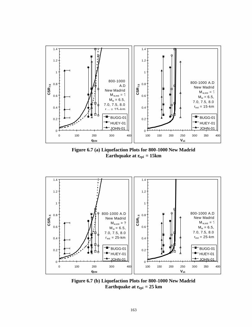
163
Figure 6.7 (a) Liquefaction Plots for 800-1000 New Madrid Earthquake at repi = 15km
Figure 6.7 (b) Liquefaction Plots for 800-1000 New Madrid Earthquake at repi = 25 km
0
0.2
0.4
0.6
0.8
1
1.2
1.4
0 100 200 300 400
qt1N
CS
R7.
5
BUGG-01
HUEY-01JOHN-01
800-1000 A.D
New MadridM w,est = ?Mw = 6.5,
7.0, 7.5, 8.0rest = 15-km
0
0.2
0.4
0.6
0.8
1
1.2
1.4
100 150 200 250 300 350 400
Vs1C
SR
7.5
BUGG-01
HUEY-01JOHN-01
800-1000 A.DNew Madrid
M w,est = ?Mw = 6.5,
7.0, 7.5, 8.0rest = 15-km
0
0.2
0.4
0.6
0.8
1
1.2
1.4
0 100 200 300 400
qt1N
CS
R7
.5
BUGG-01HUEY-01
JOHN-01
800-1000 A.DNew Madrid
Mw,est = ?M w = 6.5,
7.0, 7.5, 8.0rest = 25-km
0
0.2
0.4
0.6
0.8
1
1.2
1.4
100 150 200 250 300 350 400
Vs1
CS
R7
.5
BUGG-01HUEY-01
JOHN-01
800-1000 A.DNew Madrid
M w,est = ?Mw = 6.5,
7.0, 7.5, 8.0rest = 25-km

164
Figure 6.8 (a) Liquefaction Plots for 1400-1600 New Madrid Earthquake at repi = 15km
Figure 6.8 (b) Liquefaction Plots for 1400-1600 New Madrid Earthquake at repi = 25 km
0
0.2
0.4
0.6
0.8
1
1.2
1.4
0 100 200 300 400
qt1N
CS
R7.
5
DODD-01YARB-01
1400-1600 A.DNew Madrid
M w,est = ?Mw = 6.5, 7.0,
7.5, 8.0rest = 15-km
0
0.2
0.4
0.6
0.8
1
1.2
1.4
100 150 200 250 300 350 400Vs1
CS
R7.
5
DODD-01YARB-01
1400-1600 A.DNew Madrid
M w,est = ?Mw = 6.5, 7.0,
7.5, 8.0rest = 15-km
0
0.2
0.4
0.6
0.8
1
1.2
1.4
0 100 200 300 400
qt1N
CS
R7.
5
DODD-01YARB-01
1400-1600 A.DNew Madrid
M w,est = ?M w = 6.5, 7.0,
7.5, 8.0rest = 25-km
0
0.2
0.4
0.6
0.8
1
1.2
1.4
100 150 200 250 300 350 400
Vs1
CS
R7.
5
DODD-01YARB-01
1400-1600 A.DNew Madrid
M w,est = ?M w = 6.5, 7.0,
7.5, 8.0rest = 25-km

165
Figure 6.9 Liquefaction Plots for December 1811 New Madrid Earthquake
0
0.2
0.4
0.6
0 50 100 150 200 250 300 350 400
qt1N
CS
R7.
5
3MS617-A
YARB-01MEMPH-G
MEMPH-HSFSR-01
SFOR-01
December 1811New Madrid, MO
Mw,est = 7.9Mw = 6.5, 7.0, 7.5, 7.9
repi,est = 40- to 90-km
0
0.2
0.4
0.6
100 150 200 250 300 350 400
Vs1 (m/s)
CS
R7.
5
3MS617-A
YARB-01MEMPH-G
MEMPH-HSFSR-01
SFOR-01
December 1811New Madrid, MO
Mw,est = 7.9Mw = 6.5, 7.0, 7.5, 7.9
repi,est = 40- to 90-km

166
Figure 6.10 Liquefaction Plots for January 1812 New Madrid Earthquake
0
0.2
0.4
0.6
0 50 100 150 200 250 300 350 400
qt1N
CS
R7.
53MS617-A
YARB-01
January 1812New Madrid, MO
Mw,est = 7.6Mw = 6.5, 7.0, 7.6, 8.0
repi,est = 40- to 45-km
0
0.2
0.4
0.6
100 150 200 250 300 350 400
Vs1 (m/s)
CS
R7.
5
3MS617-A
YARB-01
January 1812New Madrid, MO
Mw,est = 7.6Mw = 6.5, 7.0, 7.6, 8.0
repi,est = 40- to 45-km
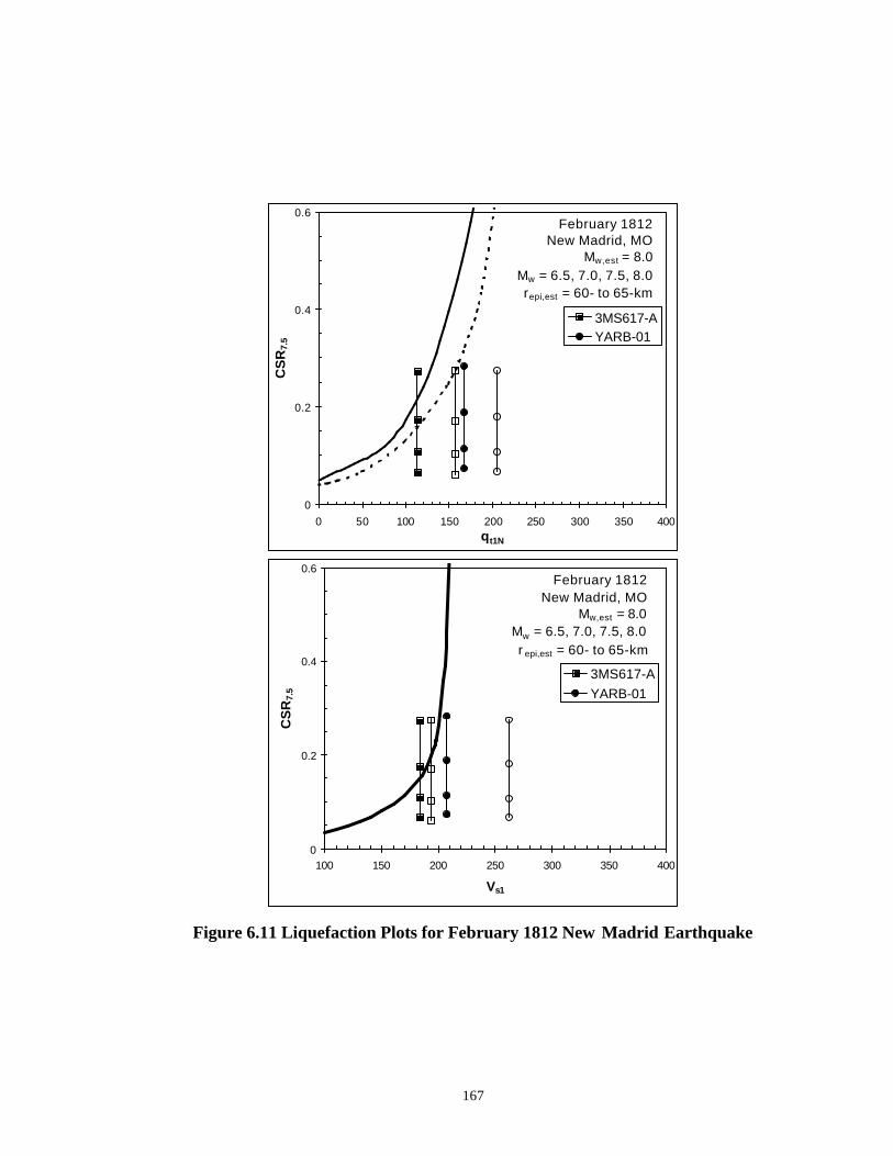
167
Figure 6.11 Liquefaction Plots for February 1812 New Madrid Earthquake
0
0.2
0.4
0.6
0 50 100 150 200 250 300 350 400qt1N
CS
R7.
5
3MS617-AYARB-01
February 1812New Madrid, MO
Mw,est = 8.0Mw = 6.5, 7.0, 7.5, 8.0repi,est = 60- to 65-km
0
0.2
0.4
0.6
100 150 200 250 300 350 400
Vs1
CS
R7.
5
3MS617-AYARB-01
February 1812New Madrid, MO
Mw,est = 8.0Mw = 6.5, 7.0, 7.5, 8.0r epi,est = 60- to 65-km

168
Figure 6.12 Liquefaction Plots for September1886 Charleston, SC Earthquake
0
0.2
0.4
0.6
0.8
1
1.2
1.4
0 50 100 150 200 250 300 350 400qt1N
CS
R7.
5
TIS-01HW-4
September 1886Charleston, SC
Mw,est = 7.0Mw = 6.0, 6.5, 7.0,
7.5 repi,est = 5- to 10-km
0
0.2
0.4
0.6
0.8
1
1.2
1.4
100 150 200 250 300 350 400
Vs1
CS
R7.
5
TIS-01
HW-4
September 1886Charleston, SC
Mw,est = 7.0Mw = 6.0, 6.5, 7.0, 7.5
repi,est = 5- to 10-km

169
6.4 Arias Intensity based Method
Results of Arias intensity-based analysis for soils in Mid-America will be
presented on charts comparing normalized in-situ test parameters to Arias Intensity, Ihb.
Sites and analyzed data will be presented on figures separated into earthquake events.
Figure 6.13 shows a sample Arias intensity-based analysis chart from this study, with
pertinent information.
Utilizing the methods presented in Figure 6.13, a critical moment magnitude will
be selected for each method, each site, and each earthquake. Critical layers are analyzed
at constant source to site distance. Utilizing magnitude dependent Arias intensity
attenuation relationships, the induced Ihb becomes solely a function of earthquake
magnitude. An Ihb line will be vertically increasing with magnitude for a critical soil
layer of constant properties. The critical magnitude represents the intersection of the Ihb
line with the Arias intensity resistance. For this study, Equation 4.28 will represent the
Arias intensity resistance. This critical magnitude represents a factor of safety near unity
that would cause borderline liquefaction. Figures 6.14 through 6.19 display the results of
Arias intensity-based analyses for six different earthquakes.

170
Figure 6.13. Key Aspects of Arias Intensity-based Analysis Charts for This Study
0.1
1
10
100
0 100 200 300 400
qt1N
Ihb (m
/s)
BUGG-01
HUEY-01
JOHN-01
800-1000 A.DNew Madrid
Mw,est = ?
Mw = 6.5, 7.0, 7.5, 8.0
rest = 25-km8.0 7.5 7.0 6.5 Mw
Legend of sites studied. Solid symbols represent first critical layer from pair. Hollow points represent second critical layer.
Earthquake induced Ihb
Averaged resistance parameter
Earthquake Date
Earthquake Location
Estimated Moment Magnitude
Range of Moment Magnitude analyzed
Arias Resistance from Eq. 4.28
Arias Resistance (Kayen & Mitchell, 1997)
1b
Critical Magnitude of about 6.9
Critical Magnitude of about 7.1
Magnitude dependent Ihb line
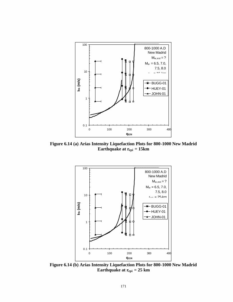
171
Figure 6.14 (a) Arias Intensity Liquefaction Plots for 800-1000 New Madrid
Earthquake at repi = 15km
Figure 6.14 (b) Arias Intensity Liquefaction Plots for 800-1000 New Madrid Earthquake at repi = 25 km
0.1
1
10
100
0 100 200 300 400
qt1N
Ihb (m
/s)
BUGG-01
HUEY-01JOHN-01
800-1000 A.DNew Madrid
Mw,est = ?
Mw = 6.5, 7.0, 7.5, 8.0
rest = 15-km
0.1
1
10
100
0 100 200 300 400
qt1N
Ihb (m
/s)
BUGG-01HUEY-01
JOHN-01
800-1000 A.DNew Madrid
Mw,est = ?
Mw = 6.5, 7.0, 7.5, 8.0
rest = 25-km

172
Figure 6.15 (a) Arias Intensity Liquefaction Plots for 1400-1600 New Madrid
Earthquake at repi = 15km
Figure 6.15 (b) Arias Intensity Liquefaction Plots for 1400-1600 New Madrid Earthquake at repi = 25 km
0.1
1
10
100
0 50 100 150 200 250 300 350 400
qt1N
I hb
(m/s
)
DODD-01YARB-01
1400-1600 A.DNew Madrid
Mw,est = ?
Mw = 6.5, 7.0, 7.5, 8.0
rest = 15-km
0.1
1
10
100
0 50 100 150 200 250 300 350 400
qt1N
I hb
(m/s
)
DODD-01YARB-01
1400-1600 A.DNew Madrid
Mw,est = ?
Mw = 6.5, 7.0, 7.5, 8.0
rest = 25-km

173
Figure 6.16 Arias Intensity Liquefaction Plots for December 1811
New Madrid Earthquake
Figure 6.17 Arias Intensity Liquefaction Plots for January 1812 New Madrid Earthquake
0.01
0.1
1
10
100
0 50 100 150 200 250 300 350 400
qt1N
Ihb (m
/s)
3MS617-A
YARB-01MEMPH-GMEMPH-H
SFSR-01
SFOR-01
December 1811New Madrid, MO
Mw,est = 7.9
Mw = 6.5, 7.0, 7.5, 7.9
repi,est = 40- to 90-km
0.1
1
10
100
0 50 100 150 200 250 300 350 400
qt1N
Ihb (m
/s)
3MS617-AYARB-01
January 1812New Madrid, MO
Mw,est = 7.6
Mw = 6.5, 7.0, 7.6, 8.0
repi,est = 40- to 45-km

174
Figure 6.18 Arias Intensity Liquefaction Plots for February 1812 New Madrid Earthquake
Figure 6.19 Arias Intensity Liquefaction Plots for Septemeber 1886
Charleston, SC Earthquake
0.01
0.1
1
10
100
0 50 100 150 200 250 300 350 400
qt1N
I hb
(m/s
)3MS617-AYARB-01
February 1812New Madrid, MO
Mw,est = 8.0
Mw = 6.5, 7.0, 7.5, 8.0
repi,est = 60- to 65-km
0.1
1
10
100
0 50 100 150 200 250 300 350 400
qt1N
I hb (m
/s)
TIS-01HW-4
September 1886Charleston, SC
Mw,est = 7.0
Mw = 6.0, 6.5, 7.0, 7.5
repi,est = 5- to 10-km

175
6.5 Cyclic Strain Based Method
Cyclic strain based analysis procedures estimate soil properties from in-situ test
parameters and incorporate the results in a rational framework for liquefaction analysis,
rather than simplified charts. Cyclic strain methods are presented in detail in Chapter 4,
but pertinent aspects will be discussed here. Shear modulus is determined from shear
wave velocity (Eq. 2.3 & 2.4), and a modified form of the Seed & Idriss (1971)
simplified procedures is utilized to estimate induced shear strain levels (Eq. 4.17). A
modified hyperbola (Eq. 2.6) is used for modulus reduction schemes incorporated into the
analysis. The critical number of cycles to induce liquefaction, nt, is determined as a
function of strain level and Ko (Eq. 4.23). Therefore, this parameter is controlled by cone
tip resistance as well as shear wave velocity for the analysis procedures used here. This
section will present results from cyclic strain-based analysis on the 22 critical layers
presented in the previous section. Soil layer parameters are presented in Table 6.2, and
average SCPTu parameters are presented in Table 6.3.
Results of cyclic strain-based analysis will be presented on charts comparing
normalized in-situ test parameters to the ratio number of earthquake cycles (n) to the
number of cycles to failure (nt). Since this method combines results from both shear
wave velocity and cone tip resistance, the two charts are not independent of each other as
they are for cyclic stress ratio analyses. Separate charts are presented for direct
comparison of stress and strain methods. While this method is capable of predicting pore
pressure generation and initial liquefaction, graphical representation of number of cycles
compared to critical number of cycles presents similar information in a clearer manner.

176
At initial liquefaction, n/nt will be equal to unity just as pore pressure ratio (ru; Fig. 4.9).
Sites and analyzed data will be presented on figures separated into earthquake events.
Figure 6.20 shows a sample cyclic strain-based analysis chart from this study, with
pertinent information.
Utilizing the methods presented in Figure 6.20, a critical moment magnitude will
be selected for each site and each earthquake. Critical layers are analyzed at constant
source to site distance. Utilizing magnitude dependent acceleration attenuation
relationships, the acceleration at the site is solely a function of earthquake magnitude at
constant source to site distance. Induces strain levels, and cycles to failure (nt) will be
constant for each soil layer, and the equivalent number of cycles (n) will be a function of
the earthquake magnitude. Therefore, the graphical representation of data in Figures 6.21
to 6.26 will be a function of earthquake magnitude and layer properties. The n/nt ratio
will be zero if the induced strain levels are below the plastic threshold strain, γtp. A line
will be vertically increasing with magnitude for a critical soil layer of constant properties
once γtp is exceeded. The critical magnitude represents the intersection of the n/nt line
with the pore pressure ratio at initial liquefaction (ru = 1). This critical magnitude can be
associated with a factor of safety near unity that would cause borderline liquefaction.
Figures 6.21 through 6.26 display the results of cyclic strain-based analyses for six
different earthquakes.

177
Figure 6.20. Key Aspects of Cyclic Strain based Analysis Charts for This Study
0
0.2
0.4
0.6
0.8
1
1.2
1.4
1.6
1.8
2
0 50 100 150 200 250 300 350 400
qt1N
n/nt
3MS617-A
YARB-01
January 1812New Madrid, MO
Mw,est = 7.6Mw = 6.5, 7.0, 7.6, 8.0repi,est = 40- to 45-km
8.0
Mw Legend of sites studied. Solid symbols represent first critical layer from pair. Hollow points represent second critical layer.
Earthquake induced n/nt ratio
Averaged resistance parameter
Earthquake Date
Earthquake Location
Estimated Moment Magnitude
Range of Moment Magnitude analyzed
Critical Magnitude of
about 7.2
Critical Magnitude of about 7.2
Magnitude dependent n/nt line
7.5 7.0 6.5
Initial Liquefaction

178
Figure 6.21 (a) Cyclic Strain Liquefaction Plots for 800-1000 New Madrid Earthquake at repi = 15km
Figure 6.21 (b) Cyclic Strain Liquefaction Plots for 800-1000 New Madrid Earthquake at repi = 25 km
0
0.2
0.4
0.6
0.8
1
1.2
1.4
1.6
1.8
2
0 100 200 300 400
qt1N
n/n t
BUGG-01HUEY-01
JOHN-01
800-1000 A.D
New MadridM w,est = ?Mw = 6.5,
7.0, 7.5, 8.0
0
0.2
0.4
0.6
0.8
1
1.2
1.4
1.6
1.8
2
100 150 200 250 300 350 400
Vs1n/
n t
BUGG-01HUEY-01
JOHN-01
800-1000 A.D
New MadridM w,est = ?Mw = 6.5,
7.0, 7.5, 8.0
0
0.2
0.4
0.6
0.8
1
1.2
1.4
1.6
1.8
2
0 100 200 300 400
qt1N
n/n t
BUGG-01HUEY-01
JOHN-01
800-1000 A.D
New Madrid Mw,est = ?
M w = 6.5, 7.0, 7.5, 8.0
0
0.2
0.4
0.6
0.8
1
1.2
1.4
1.6
1.8
2
100 150 200 250 300 350 400
Vs1
n/n t
BUGG-01HUEY-01
JOHN-01
800-1000 A.D
New MadridM w,est = ?Mw = 6.5,
7.0, 7.5, 8.0

179
Figure 6.22 (a) Cyclic Strain Liquefaction Plots for 1400-1600 New Madrid Earthquake at repi = 15km
Figure 6.22 (b) Cyclic Strain Liquefaction Plots for 1400-1600 New Madrid Earthquake at repi = 25 km
0
0.2
0.4
0.6
0.8
1
1.2
1.4
1.6
1.8
2
0 100 200 300 400
qt1N
n/n t
DODD-01YARB-01
1400-1600 A.DNew Madrid
M w,est = ?M w = 6.5, 7.0,
7.5, 8.0rest = 15-km
0
0.2
0.4
0.6
0.8
1
1.2
1.4
1.6
1.8
2
100 150 200 250 300 350 400Vs1
n/n t
DODD-01
YARB-01
1400-1600 A.DNew Madrid
Mw,est = ?Mw = 6.5, 7.0,
7.5, 8.0rest = 15-km
0
0.2
0.4
0.6
0.8
1
1.2
1.4
1.6
1.8
2
0 100 200 300 400
qt1N
n/n t
DODD-01YARB-01
1400-1600 A.DNew Madrid
Mw,est = ?Mw = 6.5, 7.0,
7.5, 8.0rest = 25-km
0
0.2
0.4
0.6
0.8
1
1.2
1.4
1.6
1.8
2
100 150 200 250 300 350 400
Vs1
n/n t
DODD-01YARB-01
1400-1600 A.DNew Madrid
Mw,est = ?M w = 6.5, 7.0,
7.5, 8.0rest = 25-km

180
Figure 6.23. Cyclic Strain Liquefaction Plots for December 1811 New Madrid Earthquake
0
0.2
0.4
0.6
0.8
1
1.2
1.4
1.6
1.8
2
0 50 100 150 200 250 300 350 400
qt1N
n/n t
3MS617-A
YARB-01MEMPH-G
MEMPH-HSFSR-01
SFOR-01
December 1811New Madrid, MO
Mw,est = 7.9Mw = 6.5, 7.0, 7.5, 7.9
repi,est = 40- to 90-km
0
0.2
0.4
0.6
0.8
1
1.2
1.4
1.6
1.8
2
100 150 200 250 300 350 400
Vs1 (m/s)
n/n
t
3MS617-AYARB-01
MEMPH-GMEMPH-H
SFSR-01SFOR-01
December 1811New Madrid, MO
Mw,est = 7.9Mw = 6.5, 7.0, 7.5, 7.9
repi,est = 40- to 90-km

181
Figure 6.24 Cyclic Strain Liquefaction Plots for January 1812 New Madrid Earthquake
0
0.2
0.4
0.6
0.8
1
1.2
1.4
1.6
1.8
2
0 50 100 150 200 250 300 350 400
qt1N
n/n t
3MS617-AYARB-01
January 1812New Madrid, MO
Mw,est = 7.6Mw = 6.5, 7.0, 7.6, 8.0
repi,est = 40- to 45-km
0
0.2
0.4
0.6
0.8
1
1.2
1.4
1.6
1.8
2
100 150 200 250 300 350 400
Vs1 (m/s)
n/n
t
3MS617-A
YARB-01
January 1812New Madrid, MO
Mw,est = 7.6Mw = 6.5, 7.0, 7.6, 8.0
repi,est = 40- to 45-km

182
Figure 6.25 Cyclic Strain Liquefaction Plots for February 1812 New Madrid Earthquake
0
0.2
0.4
0.6
0.8
1
1.2
1.4
1.6
1.8
2
0 50 100 150 200 250 300 350 400
qt1N
n/n t
3MS617-AYARB-01
February 1812New Madrid, MO
Mw,est = 8.0Mw = 6.5, 7.0, 7.5, 8.0
repi,est = 60- to 65-km
0
0.2
0.4
0.6
0.8
1
1.2
1.4
1.6
1.8
2
100 150 200 250 300 350 400
Vs1 (m/s)
n/n
t
3MS617-A
YARB-01
February 1812New Madrid, MO
Mw,est = 8.0Mw = 6.5, 7.0, 7.5, 8.0
repi,est = 60- to 65-km

183
Figure 6.26 Cyclic Strain Liquefaction Plots for September 1886 Charleston, SC Earthquake
0
0.2
0.4
0.6
0.8
1
1.2
1.4
1.6
1.8
2
0 50 100 150 200 250 300 350 400qt1N
n/n
t
TIS-01HW-4
September 1886Charleston, SC
Mw,est = 7.0Mw = 6.0, 6.5, 7.0, 7.5
r epi,est = 5- to 10-km
0
0.2
0.4
0.6
0.8
1
1.2
1.4
1.6
1.8
2
100 150 200 250 300 350 400
Vs1 (m/s)
n/n t
TIS-01HW-4
September 1886Charleston, SC
Mw,est = 7.0Mw = 6.0, 6.5, 7.0, 7.5
r epi,est = 5- to 10-km

184
6.6 Comparison of Methods
One objective of this study was to assess the application of current liquefaction
analysis methods developed for interplate earthquakes, to the anticipated motions
resulting from an intraplate event in Mid-America. Four frameworks for liquefaction
assessment have been applied to the field data from 6 earthquakes.
1. Cyclic stress-based method for cone tip resistance;
2. Cyclic stress-based method for shear wave velocity;
3. Arias intensity-based method for cone tip resistance;
4. Cyclic strain-based method utilizing both shear wave velocity and cone tip resistance.
Critical magnitudes determined for each scenario, as discussed in the previous three
sections, are presented in Table 6.5. Table 6.6 displays the comparison of each of the
analysis methods.
In general, each method compares well with each other, except the cyclic stress
method based on shear wave velocity sometimes predicts higher liquefaction resistance
and sometimes predicts lower resistance. Discrepancies have been shown when directly
comparing the small strain property of shear wave velocity to the large strain phenomena
of liquefaction (Roy et al., 1997). Even though the CRR curve for the shear wave
velocity method was based on cyclic strain theory (Andrus & Stokoe, 1997), the effects
of aging and cementation may significantly increase Vs, but are difficult to assess. The
cyclic strain based procedures are strongly controlled by the stiffness determined from
shear wave velocity methods. The theoretical cyclic strain framework, which

185
Table 6.5. Inferred Minimum Magnitude to Cause Liquefaction
Critical Magnitude Sounding repi,est Cyclic Stress Arias
Intensity Cyclic Strain
qc1 Vs1 qc1 New Madrid 800 – 1000
BUGG-01a 15 / 25 7.0 7.4 Y Y 6.7 7.1 Y 6.8 BUGG-01b 15 / 25 7.5 7.7 7 7.5 7.0 7.4 6.6 7.1 HUEY-01a 15 / 25 6.7 7.2 Y 6.5 6.5 6.7 6.8 7.4 HUEY-01b 15 / 25 8.0+ N Y 6.5 6.5 6.7 6.8 7.4 JOHN-01a 15 / 25 Y Y Y Y Y Y Y Y JOHN-01b 15 / 25 7.0 7.5 N N 6.7 7.1 7.1 7.5
New Madrid 1400-1600 YARD-01a 15 / 25 6.5 7.0 Y 6.5 6.6 7.0 6.6 7.1 YARB-01b 15 / 25 7.5 7.8 Y 6.6 7 7.4 7.1 7.5 DODD-01a 15 / 25 6.5 7.0 Y Y 6.6 6.9 Y 6.5 DODD-01b 15 / 25 6.5 7.0 N N 6.7 7.0 6.8 7.3
New Madrid December 1811; Mw,est = 7.9 MEMPH-G1 75 N 7.5 7.7 ru = 0.2 @ 7.9 MEMPH-G2 75 N N N N
SFSR-01 70 N 7.6 7.9+ ru = 0.04 @ 7.9 MEMPH-H1 90 N 7.6 7.7 ru = 0.04 @ 7.9 MEMPH-H2 90 N 7.9 N ru = 0.1 @ 7.9
SFOR-01 40 7.5 N 7.1 ru = 0.12 @ 7.9 YARB-01a 60 8.0+ 7.6 7.7 ru = 1.0 @ 7.9 YARB-01b 60 N N N ru = 0.14 @ 7.9 3MS617-A1 65 7.5 7.1 7.5 ru = 1.0 @ 7.9 3MS617-A2 65 N 7.4 7.7 ru = 1.0 @ 7.9
New Madrid January 1812; Mw,est = 7.6 YARB-01a 45 7.6 7.0 7.4 7.6 YARB-01b 45 N N 7.8 ru = 0.6 @ 8.0 3MS617-A1 40 6.8 6.6 7.1 7.2 3MS617-A2 40 7.6 6.8 7.3 7.2
New Madrid February 1812, Mw,est = 8.0 YARB-01a 65 N 7.7 7.7 ru = 1.0 @ 8.0 YARB-01b 65 N N N ru = 0.1 @ 8.0 3MS617-A1 60 7.4 7.1 7.4 7.6 3MS617-A2 60 8.0 7.3 7.6 7.6
Charleston, SC September 1886, Mw,est = 7.0 HW-4a 10 Y N 6.2 6.9 HW-4b 10 Y N Y 7.1 TIS-01a 5 Y Y Y 6.2 TIS-01b 5 Y N Y 6.7
Y - critical Mw < 6.0; N - Critical Mw > 8.0

186
Table 6.6. Comparison of Simplified Liquefaction Analysis Methods
qc1N, CSR
Vs1, CSR qc1N, Arias Cyclic Strain
qc1N, CSR the qc method typically predicted higher Mw than the Vs method
agreed well throughout
The methods agreed fairly well, except in Charleston, SC
Vs1, CSR
the qc method typically predicted higher Mw than the Vs method
The cyclic strain method predicted a high Mw, except in Charleston, SC
qc1N, Arias
agreed well throughout
Cyclic Strain
incorporates modulus reduction with increasing shear strain, appears to account for Vs-
liquefaction strain level incompatibility.
Considering the analysis methods used input ground motions of a similar original
(e.g. Attenuation relationships based on Herrmann & Akinci, 1999 Modified USGS M3
model), the relative critical magnitudes to induce liquefaction should be similar. Ground
motion differences may result from magnitude scaling factors and Arias Intensity
attenuation relationships. Figure 6.25 compares lower bound critical magnitudes
necessary for liquefaction to previous estimations of magnitude in the New Madrid

187
1 Marginal liquefaction represents denser critical layers from liquefaction sites Figure 6.25. Comparison of Lower Bound Magnitude Required for Liquefaction to
Previous Estimations of Moment Magnitude (NMSZ)
6
7
8
9
6 7 8 9
Mw,crit
Mw
,es
t
CSR, qc1N(liquefy)
CSR qc1N(marginal)CSR, Vs1(liquefy)CSR, Vs1(marginal)Arias, qc1N(liquefy)Arias, qc1N(marginal)Cyclic Strain(liquefy)Cyclic Strain(marginal)
Liquefaction Likely
Liquefaction Not Likely

188
seismic zone. Data are presented from critical layers at sites that showed surface
evidence of liquefaction. The solid symbols represent the loose critical layers with a high
liquefaction potential, while the open symbols represent the denser critical layers with a
lower liquefaction potential. Since extensive liquefaction was observed within the
NMSZ, it is expected that the earthquake magnitude would be higher than the lower
bound critical magnitude. From the data in this figure, marginal, denser layers, appear to
be susceptible to liquefaction as well. If it is considered that the loose layer was formed
by porewater migrating from the dense layer and becoming trapped under a silty clay cap,
it would be expected that the dense layer liquefied during the earthquake event.
Considering the uncertainty associated with ground motion parameters used in this study,
current liquefaction assessment methods appear to be appropriate for analysis in Mid-
America.

189
CHAPTER 7
CONCLUSIONS AND FUTURE WORK
7.1. Conclusions
In-situ geotechnical site characterization by the seismic piezocone provides a
number of parameters that can be used for liquefaction assessment and site response
analysis.
• The frequency of readings (at least every 50 mm) and the four independent
measurements (qt, fs, u2, and Vs) recorded in a SCPTu sounding provide excellent
stratigraphic profiling capabilities necessary to identify “loose” clean sands and silty
sands below the groundwater table which are potentially susceptible to liquefaction.
Penetration porewater pressure measurements at the u2 position provide a reading of
near hydrostatic water pressures in clean sands that can be used to identify the water
table depth, which is a necessary facet of any liquefaction investigation.
• Direct liquefaction analysis can be performed using cyclic stress based procedures for
normalized cone tip resistance and normalized shear wave velocity. Arias intensity
methods, which are independent of the uncertainty associated with arbitrary
magnitude scaling factors, are also available for normalized cone tip resistance.
These methods generally appeared to accurately assess liquefaction hazards at Mid-
America, considering the uncertainty in ground motion parameters. Some
inconsistencies were noticed using shear wave velocity methods, which may result

190
from strain incompatible between shear wave velocity measurements (small-strain)
and liquefaction behavior (large strain).
• Rational liquefaction analysis can be performed using cyclic strain based procedures.
Small strain stiffness is directly determined from the seismic cone, and in-situ state of
the soil can be evaluated from CPT tip resistance. Using empirical- or laboratory-
determined shear modulus reduction schemes bridge the gap between small- and
large-strain behavior.
While there is redundancy in analysis, there is still little confidence in what can be
concluded from these studies. Uncertainty is inherent in the analysis since procedures
were developed primarily for interplate earthquakes from China, Japan, and California,
and have not been calibrated for large intraplate events in Mid-America. Additional
uncertainty exists from the selection of ground motion parameters in Mid-America. A
model based on the depth and stiffness of the soil column was used to generate ground
motion parameters for this study, but this model does not incorporate the nonlinear soil
properties that will affect ground motions for a large event. Potential for amplification or
damping of motions by the deep soil column will control critical ground parameters used
for analysis. Attenuation of ground motions between epicentral distances of about 5- to
70-km is significant. Therefore accurate evaluation of the source-to-site distance is
paramount in liquefaction studies.
It can be inferred from the layering and consistency characteristics of soil deposits at
liquefaction sites in the New Madrid seismic zone that liquefaction resulted in loose
sands near the surface from excess porewater pressures becoming trapped below low

191
permeability clay or silt layers. While analyses from this study evaluated two separate
layers per sounding, it is likely that liquefaction occurred throughout the depth of the
deposit. This would result in the observed profile of a low permeability silty clay cap,
over loose shallow sands, over densified deeper sands.
7.2 Future Work
The data available from the seismic piezocone penetration test provide the
stiffness parameters necessary to perform a site-specific response analysis of ground
motions, such as SHAKE (Fig. 7.1). This would eliminate the empirical rd and rb stress
reduction coefficients used in the simplified procedures. Strain levels for use in cyclic
strain based methods can also be generated from a site-specific analysis. Assessment of
analysis methods presented in this study utilizing equivalent linear and nonlinear models
may additional provide insight into the liquefaction behavior of deposits profiled in this
study.
Questions often arise as to the applicability of using post earthquake field
performance data to estimate pre-earthquake sand-state. There is likely significant
disturbance, whether it is densification of a loose layer through subsidence or loosening
of a dense layer from pore pressure migration into that layer. Pre- and post-earthquake
studies have been performed at liquefaction sites (e.g., Frost et al., 1993; Chameau et al.,
1998) to evaluate potential earthquake effects on deposits. Additional studies in Mid-
America may provide additional insight into the effects of liquefaction induced
densification on penetration resistance and soil stiffness, especially at sites where re-
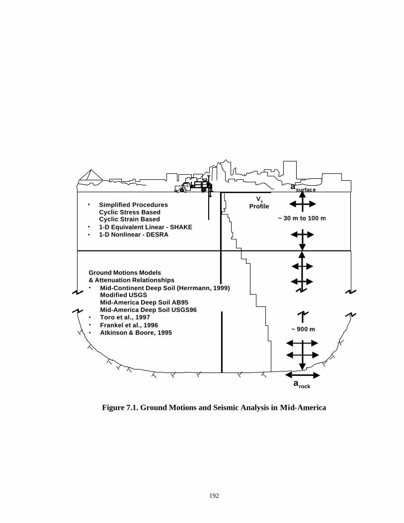
192
• Simplified ProceduresCyclic Stress BasedCyclic Strain Based
• 1-D Equivalent Linear - SHAKE• 1-D Nonlinear - DESRA
~ 30 m to 100 m
~ 900 m
Ground Motions Models& Attenuation Relationships• Mid-Continent Deep Soil (Herrmann, 1999)
Modified USGSMid-America Deep Soil AB95Mid-America Deep Soil USGS96
• Toro et al., 1997• Frankel et al., 1996• Atkinson & Boore, 1995
arock
asurface
Vs
Profile
Figure 7.1. Ground Motions and Seismic Analysis in Mid-America

193
liquefaction is evident (e.g. sand dikes venting through existing liquefaction induced sand
dikes).
From laboratory and field investigations it appears that sands from selected sites
from Mid-America are relatively clean (FC < 5 %). It is desirable to verify these
predictions using conventional drilling and sampling techniques. Additionally,
laboratory testing of strength, stiffness, and critical state properties of sands throughout
Mid-America could be used to supplement the data collected in this study. Cyclic
laboratory testing on disturbed as well as frozen specimens would supplement the
database of Japanese sites used to generate the limiting value of CPT tip resistance for
cyclic resistance curves used in this study.
Difficulties arise when deciding upon the input ground motions for site specific
analysis, since no strong ground motion data is available for the Mid-America region.
Depth of analysis is another concern for site response studies in the 600- to 1000-m deep
soils of the Mississippi River Valley and Atlantic Coastal Plain. It is preferable to use
actual time histories rather than synthetic ground motions based on stochastic white noise
(Youd, 1997), but actual ground motions are not available for intraplate earthquakes in
Mid-America. Continued ground motion studies in Mid-America are of great importance
for earthquake engineering.
Since the uncertainty associated with ground motions in the Mid-America region
greatly effects the outcome of liquefaction analyses, a direct assessment of liquefaction
resistance of a deposit is desirable. The initial development of a vibrocone penetrometer
(VCPT) is ongoing through a joint project at Georgia Tech and Virginia Tech (Schneider

194
Figure 7.2. Static piezovibrocone and seismic piezocone soundings at Hollywood Ditch, Charleston, SC
Figure 7.3. Comparison of static and dynamic piezovibrocone soundings at Hollywood Ditch, Charleston, SC
0
2
4
6
8
10
0 5 10 15 20qc (MPa)
Dep
th B
GS
(m
)
HW - 4; Gregg In-situ
HW - 2; Static Vibrocone
0
2
4
6
8
10
0 50 100 150fs (kPa)
HW - 4; Gregg In-situ
0
2
4
6
8
10
-100 100 300um (kPa)
HW - 4; u2
HW - 2; u1
u2
u1
0
2
4
6
8
10
0 250 500Vs (m/sec)
HW - 4; Seismic CPT
SASW (Indridason,1992)
Clean Sands
Silty Sand toClayey Silt
Clean Sand to Silty Sand
Silt toSandy Silt
0
2
4
6
8
10
0 100 200 300
u1 (kPa)
HW - 1; Dynamic
HW - 2; Static
u1
0
2
4
6
8
10
0 5 10 15 20
qc (MPa)
Dep
th B
GS
(m
)
HW - 1; Dynamic Vibrocone
HW - 2; Static Vibrocone

195
et al., 1998). Initial trial field studies have been performed in Charleston, SC and
calibration chamber testing is ongoing at Virginia Tech. Preliminary results look
promising, with additional porewater pressures generated from vibratory penetration (Fig.
7.2; 7.3). Additional vibrocone testing at liquefaction sites in Mid-America will aid in
the understanding of the liquefaction response of soil in Mid-America.

196
APPENDIX I.
SOIL PROPERTIES
I.1 Overview
An introduction to engineering soil classification, effective stress-state in soils, and
engineering definitions of soil properties is presented in a framework related to
geotechnical earthquake engineering. Earthquake induced liquefaction is generally
associated with contractive granular soils, while site amplification effects are typically
seen in soft, high plasticity, clay deposits. From simplified liquefaction resistance charts
(i.e. Stark & Olson, 1995), the input parameter of fines content or mean grain diameter is
needed. Initial cyclic stress based methods were based on the belief that liquefaction is a
function of relative density (Seed & Lee, 1966). Cyclic strain based methods show the
initial build up of pore pressures is a function of small-strain shear modulus, Gmax, as well
as modulus reduction, G/Gmax. Threshold shear strains and modulus reduction appear to
be a function of plasticity, as well as other factors (Vucetic & Dobry, 1991). For the
cyclic strain method, the shape of pore pressure generation curves is expected to be a
function of current stress state as well as past effective stresses, i.e., σvo', Ko, and OCR
(Vasquez-Herrera, et al., 1988). Definitions of these properties will be presented in the
following sections.

197
I.2 Soil Characterization and Basic Properties
An engineering definition of soil type will be required for geotechnical
earthquake analyses. The most common methods have been visual and manual
classification, simple index tests, and incorporation into the unified soil classification
system (USCS). Figure I.1 displays typical laboratory classification procedures and
classification schemes. The most common way to display the results of laboratory
classification is through a grain size distribution (GSD) curve. Figure I.2 displays the
GSD for sand from a liquefaction site in Blytheville, AR, as well as a silty sand - sandy
silt from the Piedmont Province in Georgia. From this curve typical gradation properties
can be determined, and then used for soil classification.
Sieve analyses are performed following the general procedures outlined in ASTM
D422, and GSD curves can be assessed by evaluating:
• Median grain size, D50 - where D is particle diameter in millimeters and the
subscripted number represents the percentage of particles finer by weight. For this
case D50 refers to the particle size in millimeters relating to 50 percent finer by
weight;
• Effective grain size, D10 - the particle size in millimeters relating to 10 percent finer
by weight.
• Coefficient of uniformity, Cu = D60/D10;
• Coefficient of curvature, Cc = D302 / (D10�D60).

198
Figure I.1. Laboratory Soil Classification Methods
100 10 1 0.1 0.01 0.001 0.0001
300 200 50 20 5 2 0.5 0.2 0.05 0.02 0.005 0.002 0.0005 0.0002
CLAYCoarse Fine Crs Medium Fine
GRAVEL SANDSILTCOBBLES
ParticleDiameter 76.2 19.1 4.76 2.00 0.420 0.075 0.002* 0.0005(mm)
SieveSize 3 in. 3/4 in. #4 #10 #40 #200 Hydrometer Test(U.S. Standard)
* According to ASTM D653-90, the clay fraction is designated as the percentage finer than 0.002 mm, but 0.005 mmin some cases.
COLLOIDS
GWGP
SWSP
0 5 12 50 100Percent Fines
Coarse-Grained Soils Fine-Grained Soils
Du
al S
ymb
ol A-Line
Liquid Limit= 50
CLOL
MHOH
CHOH
MLOL
SMSC
GMGC
USCSSymbols:
Soil Type:G- GravelS-SandM-SiltC-ClayO-Organic
USCSSymbols:
Gradation(Sieve Analysis)W- Well GradedP-Poorly Graded
Plasticity(Atterberg Limits)H-High PlasticityL-Low Plasticity
Soak overnight in Dispersing AgentSolution (Sodium hexametaphosphate -"Calgon" 41 grams/liter)
Forms suspension ofparticles.
The hydrometer willsink deeper asparticles settle out.
No. 200
WashSamplethroughNo. 200Sieve
Dry Sample

199
Figure I.2. Grain Size Distribution Curves for two Sandy Soils
Table I.1. Grain Properties of Sandy Soils from Figure I.2
Soil D50 D10 Cu Cc Percent Fines
USCS Symbol
Piedmont 0.065 0.0013 76.9 1.73 54 SM-ML Yarbro 0.41 0.21 2.3 0.95 1 SP
The separation between coarse grained soils and fine grained soils will be 0.075
millimeters, which is related to a number 200 sieve. The separation between silt and clay
is 0.002 millimeters, and can be estimated from hydrometer analysis (ASTM D-422). For
example, the representative grain properties and associated USCS symbol for the sandy
soils in Figure I.2 are presented in Table I.1.
0
10
20
30
40
50
60
70
80
90
100
0.0010.010.1110100
Grain Size in Millimeters
Per
cen
t Fin
er b
y W
eig
ht
Piedmont Silty Sand -Sandy Silt
Yarbro ExcavationSand
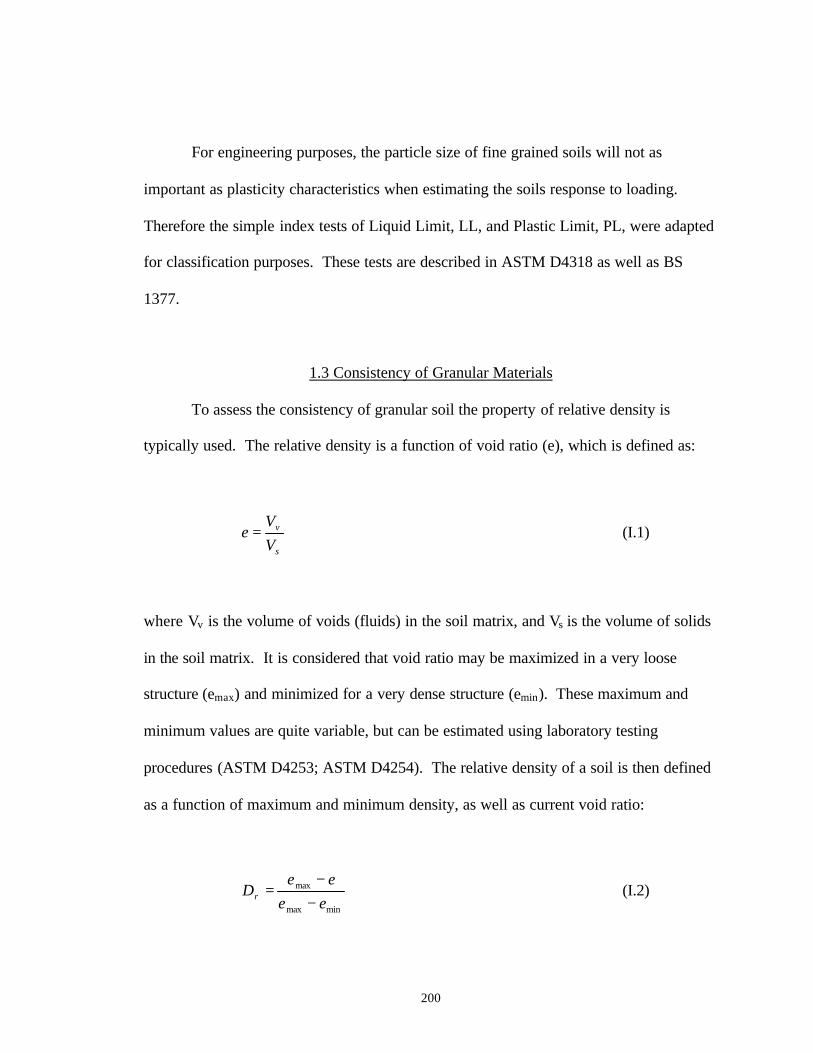
200
For engineering purposes, the particle size of fine grained soils will not as
important as plasticity characteristics when estimating the soils response to loading.
Therefore the simple index tests of Liquid Limit, LL, and Plastic Limit, PL, were adapted
for classification purposes. These tests are described in ASTM D4318 as well as BS
1377.
1.3 Consistency of Granular Materials
To assess the consistency of granular soil the property of relative density is
typically used. The relative density is a function of void ratio (e), which is defined as:
s
v
VV
e = (I.1)
where Vv is the volume of voids (fluids) in the soil matrix, and Vs is the volume of solids
in the soil matrix. It is considered that void ratio may be maximized in a very loose
structure (emax) and minimized for a very dense structure (emin). These maximum and
minimum values are quite variable, but can be estimated using laboratory testing
procedures (ASTM D4253; ASTM D4254). The relative density of a soil is then defined
as a function of maximum and minimum density, as well as current void ratio:
minmax
max
eeee
Dr −−
= (I.2)

201
To estimate the consistency of an in-situ soil deposit, relative density is often
used. If maximum and minimum void ratios are known, Dr may be determined by
estimates of in-situ void ratio. Table I.2 presents correlations between CPT tip resistance
and relative density. Table I.3 presents correlations between SCPTu measurements and
in-situ void ratio.
Table I.2. Correlations between In-Situ Dr to CPT Measurements
Relationship
Notes Reference
−
⋅1
'log68
voa
c
p
q
σ
• pa is atmospheric pressure • qc and σvo' are in the same units • based on boundary condition
uncorrected calibration chamber data
• mainly unaged clean quartz sands • to utilize field data, divide field
determined qc by Kq, where: Kq = 1 + (Dr - 30) / 300
Jamiolkowski et al., 1985b
5.0
2.01
305100
⋅
⋅OCRqc
• qc1 = qc/(σvo')0.5, where qc and σvo' are in the same units
• based on boundary condition corrected calibration chamber data
• n = 544 • unaged sands • to account for aging, divide qc1 by
CA, where:
⋅+=100
log05.02.1t
CA
Mayne & Kulhawy, 1991 Kulhawy & Mayne, 1990

202
Table I.3. Correlations between In-Situ Void Ratio and SCPTu Measurements
Relationship
Notes Reference
1.159-0.230�log(qc1)
• qc1 = qc/(σvo')0.5, where qc and σvo' are in the same units
• based on calibration chamber test data
• applicable to normally consolidated unaged, clean, quartz sands
• n = 494; r2 = 0.668
Mayne, 1995
1.232-0.245log(qc1)
• qc1 = qc/(σvo')0.5, where qc and σvo' are in the same units
• based on calibration chamber test data
• applicable to overconsolidated (OC) consolidated unaged, clean, quartz sands
• n = 149; r2 = 0.820
Mayne, 1995
1.152-0.233�log(qc1) +
0.043�log(OCR)
• qc1 = qc/(σvo')0.5, where qc and σvo' are in the same units
• based on calibration chamber test data
• applicable to unaged, clean, quartz sands
• n = 643; r2 = 0.691
Mayne, 1995
259381 1SV−
• Vs1 = Vs/(σvo')0.25, where σvo' is in
atmospheric units and Vs is in m/s • based on laboratory tests on Ottawa
sand
Robertson et al., 1995
188311 1SV−
• Vs1 = Vs/(σvo')0.25, where σvo' is in
atmospheric units and Vs is in m/s • tests on Syncrude sand
Cunning et al., 1995
I.4 Effective Stress State in Soils
Saturated soil response to shearing will be controlled by mechanics of the soil
structure as well as stress-state from induced water pressures. The particulate matrix of a

203
soil will increase in strength with increased confining stress. As depth increases so will
the vertical confining stress:
∫ ⋅= dztvo γσ (I.3)
where σvo is the total vertical stress in the soil, z is depth, and γt is the total unit weight
equal to ρt � g, where ρt is the total mass density and g is the acceleration due to gravity.
Hydrostatic water pressure, uo, will increase with depth below the water table as:
uo = hwγw (I.4)
where hw is the depth below the water table and γw is the unit weight of water. The total
stress will act to confine the element, and the water pressure will act oppositely in all
directions. The pore water pressure during undrained failure will be composed of the
hydrostatic pore water pressure as well as shear- induced water pressures, ∆ushear. If the
rate of shear is slow enough to allow drainage, ∆ushear will equal zero. During loading or
the process of in-situ testing, octahedral pore pressures, ∆uoct, may be induced. The total
composite pore pressure, u, may be expressed as:
u = uo + ∆ushear + ∆uoct (I.5)

204
The strength of the soil will controlled by the effective stress, σ'vo:
σ'vo = σvo - u (I.6)
The horizontal stress will also be effected by the hydrostatic pore water pressure as:
σ'ho = σho - u (I.7)
The ratio of horizontal to vertical effective stress is known as the coefficient of lateral
stress at rest, Ko :
vo
hooK
''
σσ
= (I.8)
The coefficient of earth pressure at rest, Ko, can also be estimated by the relationship
presented by Mayne & Kulhawy (1982):
Ko = (1-sinφ')OCRsinφ' (I.9)
where OCR is the overconsolidation ratio and φ' is the effective stress friction angle.
Each of these properties will be discussed below.

205
Table I.4. Correlations between SCPTu parameters and In-Situ Stress State
Property Relationship Notes Reference σho' qc
1.6�10(1.144-0.0186�Dr) • σho' is in kPa, qc is in MPa, and Dr is in percent
• based on calibration chamber test data
• applicable to unaged, clean, quartz sands
• σho' = Ko � σvo'
Mayne, 1991
Stress History, OCR, &
Stress State, Ko
27.0
31.022.0'
192.0
OCR
ppq
Ka
vo
a
co
=
−σ
Ko = (1-
sinφ')OCRsinφ'
• pa is atmospheric pressure • based on boundary cond ition
corrected calibration chamber data
• estimate friction angle from above procedures, and iterate to solve to equations simultaneously
Mayne, 1995 Mayne & Kulhawy, 1982
Throughout a soil deposits formation and geologic history, it will undergo different
stress conditions. Increased effective stresses or apparent effective stresses on an element
of soil can result from groundwater fluctuation, aging, cementation, mechanical pre-
stressing, as well as desiccation. The preconsolidation stress, p'c is defined as the
maximum past stress the soil element has experienced throughout its history and is
commonly represented by the overconsolidation ratio, OCR:
vo
cpOCR
''
σ= (I.10)

206
From the concepts of critical state soil mechanics (CSSM), an overconsolidated soil
(OCR > 1) generally deforms elastically within the yield locus (σ' < p'c), while a normally
consolidated soil (OCR = 1) acts elasto-plastically with an expanding yield surface
(Wood, 1990). Table I.4 display correlations between SCPTu parameters and the in-situ
stress state of sands. To utilize the Ko, OCR, f' relationship presented in Mayne &
Kulhawy (1982) and Table I.4, knowledge of effective stress friction angle will be
required. This is discussed in the following section.
I.5 Strength Properties of Granular Materials
The drained strength of granular materials is typically expressed using Mohr-
Coulomb failure criteria (with effective cohesion intercept c' = 0):
τmax = (σ'vo)tanφ' (I.11)
where τmax is the maximum shear strength, and φ' is the effective stress friction angle.
Early studies of frictional resistance showed a linear increase with confining stress, but
additional consideration of the particulate nature of soils showed that friction angle is
controlled by other factors as well. Rowe (1962) showed that effective stress friction
angle in soils was a sum of a constant sliding friction, as well as void ratio dependent
particle rearrangement and dilatency. Additional studies by Lee and Seed (1967) showed
φ' to be a function of sliding friction, dilatency, crushing, and re-arrangement, which are

207
all functions of normal stress. Table I.5 displays correlations between CPT tip resistance
and effective stress friction angle, φ'.
Table I.5. Correlations between qc and φ '
Relationship
Notes Reference
⋅+
'log38.010.0arctan
vo
cqσ
• where qc and σvo' are in the same units • based on calibration chamber test data • mainly clean quartz sands • laboratory φ' from triaxial tests at chamber
σho'
Robertson & Campanella, 1983
+
⋅ 26.1
'log8.30
vo
sf
σ
• where fs and σvo' are in the same units • evaluation of lateral stress from fs
measurements • comparison with field data (SBPMT,
DMT, etc.) • Assesses disturbed Ko condition as Kp
Masood & Mitchell, 1993
( )1log116.17 co q⋅+ • qc1 = qc/(σvo')0.5, where qc and σvo' are in
the same units • based on calibration chamber test data • mainly unaged clean quartz sands • laboratory φ' from triaxial compression
tests • n = 633, r2 = 0.64
Kulhawy & Mayne, 1990
A soils stress path to failure can be plotted in p'-q space, where 3
'2'' hvp
σσ += and
)''( hvq σσ −= . A failure surface Μ is defined as a function of φ', which differs in
compression and extension. During shear, the stress state (p' and q) will move towards
this failure envelope in a manner dependant upon soil properties and type of loading. In
void ratio - stress space, a unique critical state of constant volume and unlimited shear
strain has been shown to exist (e.g., Poulos, 1981). During drained shear, a soil specimen

208
will exhibit volume change while moving towards this line. During undrained shear, a
soil element will generate excess pore water pressures to move towards failure. Studies
of laboratory tests revealed a potential surface within the failure envelope where
rearrangement of grains during shear may lead to an unstable soil structure. A collapse
surface is said to exist where loss of contact points between grains leads to structural
collapse, rapid increase in pore pressures, and flow to the critical void ratio (Alarcon-
Guzman et al., 1988). Depending upon stress conditions and type of loading, flow
structure may be more important to evaluate than the critical state line.
When subjected to earthquake shaking, collapsible soils will tend to contract,
generating positive pore pressures in the absence of drainage. As the pore water pressure
increases, the effective stress will decrease (Eq. I.6), leading to a loss of strength. When
the excess pore water pressure (∆u) equals the original effective stress, the effective stress
goes to zero (u = σvo) causing initial liquefaction (Seed & Lee, 1966).
I.6 Critical State Properties of Granular Materials
The importance of volume change characteristics of sands during shear was initially
presented in Casagrande (1936). This paper discussed that when sheared, loose and
dense soils will change volume and move towards a unique critical void ratio where
unlimited deformation is possible with no volume change. Further research showed that
the critical void ratio decreases with increasing normal stress. If the soil is saturated and
drainage is not permitted during loading, there can be no global volume change in the
specimen. Contraction and dilation tendencies will then be accounted for by pore

209
pressure response. The development of Critical State Soil Mechanics (CSSM; Roscoe,
Schofield & Wroth, 1958; Schofield & Wroth, 1968) has experimentally and numerically
quantified the presence of a critical state for soils, generally for normally consolidated
clays. Experimental validation of these concepts using sands had been limited by lack of
soil matrix compression under isotropic conditions (Wood, 1990).
The uniqueness of the critical state line for sands has been the subject of debate.
Stress controlled tests presented in Castro (1969) showed the presence two distinct
critical failure lines in e- log σ3' space, instead of a unique critical state line. An Fe line
represented a liquefaction induced flow structure, while an Se line represented steady
state deformation. The Fe line was generated by undrained and drained tests on loose
specimens, and the Se line was generated by undrained tests on dense specimens. These
lines were further defined (and renamed as the F and S lines) by the work of Alarcon-
Guzman et al. (1988). The F line represents the critical state line for sands generated
from strain softening behavior, while the S line represents strain hardening behavior.
There is an area between these two lines where quasi-steady state and limited strain
softening may occur. The difference between the S line and F line can be explained by
the development of shear bands within dilative triaxial specimens. As a dilative
specimen is sheared, a distinct failure plain will be generated. The stress-strain response
of the soil will not be controlled by the global void ratio of the specimen, but by the
interface between the two blocks separated by the shear band. This interface will be
controlled by the void ratio and confining stress within the shear band. Studies of local
void ratio in dense specimens by Desrues et al. (1996) and Frost et al. (1999) showed that

210
local void ratio within shear bands approaches that of the critical state determined from
loose specimens. Considering the critical state line from contractive tests, and the
presence of shear banding and subsequent effect of local void ratio in dilative specimens,
a unique critical state line regardless of stress path or testing procedure is accepted.
Since the slope of the critical state line has been shown to be controlled by
particle shape, and the position of the critical state line has been shown to be controlled
by gradation (Poulos et al., 1985), studies as to the effects of particle crushing have been
undertaken. Been et al. (1991) concluded that a sharp break in the slope of the critical
state line on a semi- log plot, Figure I.3a, is the result of particle crushing. In a discussion
to that paper, Verdugo (1992) presented the same data on a linear plot, Figure I.3b, and
discussed exaggeration as a result of the semi- log scale. Been (1999) determined that
curvature in the critical state line is not an issue of great importance, and there is no
theoretical reason for the log- linear relationship. Depending upon the stress range of
concern, a linear relationship or bi- linear logarithmic relationship may be desirable for
ease in mathematical interpretation. Upward curvature of the critical state line at low
stresses on a linear plot and downward curvature at high stresses on a semi- log plot
should be taken into consideration during analysis.
During undrained shear (e.g. earthquake loading) the soil element will act under a
constant volume condition, with volume change characteristics resulting in pore pressure
response. The critical state line will act as a demarcation between contractive, positive
pore pressure generation, and dilative, negative pore pressure generation. Therefore if

211
Figure I.3a. Critical state line for Toyoura and Erksak Sands on semi-log scale
Figure I.3b. Critical state line for Toyoura and Erksak Sands on linear scale
0.5
0.6
0.7
0.8
0.9
1
10 100 1000 10000
p' (kPa)
Vo
id R
atio
, e
Toyoura Sand (Verdugo& Ishihara, 1991)
Erksak Sand (Been etal., 1991)
0.5
0.6
0.7
0.8
0.9
1
0 500 1000 1500 2000 2500 3000 3500
p' (kPa)
Vo
id R
atio
, e
Toyoura Sand (Verdugo& Ishihara, 1991)
Erksak Sand (Been etal., 1991)

212
Figure I.4. State Approach to Liquefaction Assessment
0.65
0.7
0.75
0.8
1 10 100 1000
p' (kPa)
Voi
d R
atio
, e
e = Γ1 kPa - λss ln (p')
eo - ess = ψ
ContractiveLiquefaction Likely
DilativeLiquefaction Not Likely
λss
1

213
the in-situ state, e, σvo', and Ko, or state parameter, ψ, is known, an estimation of
liquefaction resistance can be determined. Concern with the utilization of remolded
laboratory specimens to soils in the field has been expressed for liquefaction analyses
(Vaid & Thomas, 1995). Lack of soil structure and aging are a concern in laboratory
specimens, as well as scale effects and natural variability. Estimation of state parameter
from in-situ tests is still developing, and is discussed in Jefferies (1999) and Shuttle &
Jefferies (1998).
I.7 Small Strain Properties
Small strain properties of shear wave velocity (Vs) and maximum shear modulus
(Gmax) were previously discussed in Chapter 2. It is desirable to measure these properties
in-situ via methods such as crosshole testing, downhole testing, spectral analysis of
surface waves, etc. If preliminary estimates of Vs and Gmax are desired and penetration
test data is available, correlations contained in Table I.6 are available for use.
Table I.9. Correlations between Cone Tip resistance and Small Strain Properties
Property Relationship Notes Reference
277�(qc)0.13(σvo')0.27
• Vs in m/s; qc and σvo' in kPa
• based on Italian sands
Baldi et al., 1989
Shear Wave Velocity, Vs
Vs1 = 102�(qc1)0.25
• Vs1 in m/s • Vs1 = Vs�(pa/σvo')0.25 • qc1 = qc (Pa/σvo')0.5 • sand field data
Robertson et al., 1992b
Vs1 = 135�(qc1)0.23
• Vs1 in m/s • site specific field data
for Alaska sand
Fear & Robertson, 1995

214
Table I.9. Continued
Vs1 = f (qc1, FR)
• based on field data • incorporated into
classification chart
Olsen, 1994
1.75(qc)0.627
• Vs in m/s; qc in kPa • based on 31 intact
and fissured clays sites
• n = 481; r2 = 0.736
Mayne & Rix, 1995
Shear Wave Velocity, Vs
14.02(qc)0.364�(eo)-0.490
• Vs in m/s; qc in kPa • based on 31 intact
and fissured clays sites
• n = 364; r2 = 0.846
Mayne & Rix, 1995
14.13�qc
0.359�eo-0.473
• Vs in m/s; qc in kPa • application to clay
soils • field data collected
from 36 clay sites • n = 406; r2 = 0.885
Hegazy & Mayne, 1995
(Gmax)1 = f (qc1, FR)
• based on field data • incorporated into
classification chart
Olsen, 1988
Small Strain
1634�(qc)0.250(σvo')0.375
• Gmax, qc, and σvo' are in kPa
• based on sand field data and calibration chamber test results
Rix & Stokoe, 1991
Stiffness, Gmax
2.78(qc)1.335
• Gmax and qc are in kPa
• based on field data from 31 clay sites
• n = 481; r2 = 0.713
Mayne & Rix, 1993
406(qc)0.695eo
-1.130 • Gmax and qc are in
kPa • based on field data
from 31 clay sites • n = 418; r2 = 0.901
Mayne & Rix, 1993

215
APPENDIX II
GROUND MOTION PARAMETERS
II.A Ground Motion Parameters
Many parameters exist which can be used to characterize earthquake related
ground motions. These include, but are not limited to, moment magnitude (Mw), peak
ground acceleration (PGA), and Arias intensity. These parameters are discussed in the
following sections.
II.B Moment Magnitude
Without modern seismographs, scales relating earthquake- induced damage to
intensity were used (e.g. Modified Mercalli, Japanese Meteorological Agency). To
quantify earthquake size measurements of earthquake magnitude were developed from
modern instrumentation, but early methods were typically empirical and device
dependant (Kramer, 1996). Some early magnitude scales include Richter Local
Magnitude, ML, Surface Wave magnitude, MS, Short Period Body Wave Magnitude, mb,
Long Period Body Wave, mB, and the Japanese Meteorological Agency magnitude,
MJMA. Since these methods are a function of measured seismic waves and not fault
rupture, they are not directly related and tend to reach a constant maximum value. Figure
II.1 displays saturation of various magnitude scales. A brief description of scales is

216
Figure II.1. Comparison of Empirical Magnitude Scales to Moment Magnitude (Idriss, 1985)
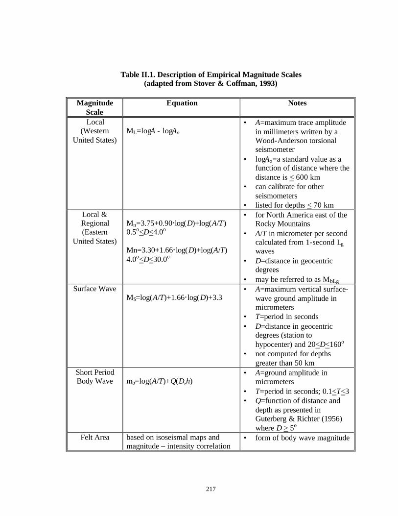
217
Table II.1. Description of Empirical Magnitude Scales (adapted from Stover & Coffman, 1993)
Magnitude
Scale Equation Notes
Local (Western
United States)
ML=logA - logAo
• A=maximum trace amplitude in millimeters written by a Wood-Anderson torsional seismometer
• logAo=a standard value as a function of distance where the distance is < 600 km
• can calibrate for other seismometers
• listed for depths < 70 km Local & Regional (Eastern
United States)
Mn=3.75+0.90�log(D)+log(A/T) 0.5o<D<4.0o Mn=3.30+1.66�log(D)+log(A/T) 4.0o<D<30.0o
• for North America east of the Rocky Mountains
• A/T in micrometer per second calculated from 1-second Lg waves
• D=distance in geocentric degrees
• may be referred to as MbLg Surface Wave
MS=log(A/T)+1.66�log(D)+3.3 • A=maximum vertical surface-
wave ground amplitude in micrometers
• T=period in seconds • D=distance in geocentric
degrees (station to hypocenter) and 20<D<160o
• not computed for depths greater than 50 km
Short Period Body Wave
mb=log(A/T)+Q(D,h)
• A=ground amplitude in micrometers
• T=period in seconds; 0.1<T<3 • Q=function of distance and
depth as presented in Guterberg & Richter (1956) where D > 5o
Felt Area based on isoseismal maps and magnitude – intensity correlation
• form of body wave magnitude

218
contained in Table II.1.
To eliminate saturation effects, a more fundamental magnitude scale based on the
seismic moment ( DAM µ=0 , where µ is the rupture strength of the material along the
fault, A is the rupture area, and D is the average amount of slip). If seismic moment is
expressed in dyne-cm, the moment magnitude, MW, can be expressed as (Kramer, 1996):
7.105.1
log 0 −=M
M W (II.1)
The moment magnitude of an earthquake will also have an influence on a number of
Figure II.2. Graphical Representation of Ground Motion Parameters
Peak Acceleration, amax
0 + 0.05
- 0.05
- 0.65 amax
+ 0.65 amax
Bracketed Duration
time (sec)
Ampl
itude
(g)

219
other ground motion properties, such as duration (e.g., Chang & Krinitzky, 1977),
significant stress cycles (e.g., Seed et al., 1985), acceleration (e.g., Toro et al., 1997), and
Arias Intensity (e.g. Kayen & Mitchell, 1997). Figure II.2 displays a graphical
representation of the ground motion parameters mentioned above.
II.C Peak Ground Acceleration
For geotechnical analyses, the peak horizontal ground acceleration (PGA or amax)
is typically used to characterize the amplitude of a particular ground motion. The vertical
component of motion is not typically used since it is usually lower than the peak
horizontal acceleration (e.g., Newmark & Hall, 1982) and gravity induced static forces
provide a substantial factor of safety against vertical motion (Kramer, 1996). If
acceleration measurements are recorded in two perpendicular directions, the vector sum
can be used to determine the amplitude and direction of motion (Kramer, 1996). Figure
II.2 displays the maximum acceleration on an example accelerogram.
The value associated with 65 percent of amax is typically associated with the
average amplitude of significant ground motion (Seed & Idriss, 1971). The earthquake
duration and number of significant stress cycles is not a function of acceleration, and thus
parameters in addition to acceleration (e.g. Magnitude Scaling Factors (MSF); Chapter 3)
are needed to characterize ground motions for simplified procedures.

220
II.D Arias Intensity
Arias intensity represents the cumulative energy per unit weight in a given
direction that is absorbed by a set of single degree of freedom oscillators (Arias, 1970).
Considering that the damping of a nonliquified soil deposit will not significantly affect
the calculation of Arias intensity, the case where the damping ratio approaches zero will
be used (Kayen & Mitchell, 1997). Horizontal Arias intensity can be calculated as the
sum of the area under acceleration time histories in the x- and y- directions:
( ) ( )dttag
dttag
IIIoo t
y
t
xyyxxh ∫∫ +=+=0
2
0
2
22ππ
(II.2)
Where Ih is the horizontal Arias intensity, Ixx is the Arias Intensity in the x direction, Iyy is
the Arias intensity in the direction perpendicular to Ixx, and ax(t) and ay(t) are the
acceleration time histories in the x and y directions respectively. The acceleration time
history values are squared for integration purposes to eliminate negative area during
integration. The values are subsequently divided by two, which negates the squared
component. It is recommended that numerical integration by the trapezoidal method be
used to determine Arias intensity (Youd et al., 1997). Since the entire acceleration time
history is accounted for, no additional parameters are necessary to characterize
earthquake motion.

221
APPENDIX III.
SEISMIC PIEZOCONE DATA COLLECTION SYSTEM AND SHEAR WAVE ANALYSIS PROCEDURES
III.A. Cone Penetrometers and Field Testing
Three electronic cone penetrometers, each manufactured by Hogentogler, were
used during the investigations. The piezocones were vertically advanced at the standard
rate of 2 cm/sec (Lunne et al., 1997) using the Georgia Tech GeoStar open chasis cone
truck. Readings of tip resistance (qc), sleeve friction (fs), inclination (i), and pore
pressure (um) were taken every 5-cm (2.5-sec).
Inside the penetrometer, approximately 25-cm behind the tip, are a velocity
geophone and an inclinometer. The inclinometer is used to assess the verticality of the
sounding to warm against excessive drift. The geophone detects vertically-propagating,
horizontally-polarized shear waves generated at the ground surface at intervals of
approximately 1-meter, corresponding to successive rod additions.
The filter elements consisted of high-density polypropylene that was saturated
with glycerin in a small vacuum chamber prior to testing. Filter elements were changed
to minimize clogging , and the cone was re-saturated between each test to ensure accurate
pore pressure data.
The data acquisition system used during testing was a commercial Hogentogler
field computer unit interfaced with the GT - GeoStar cone truck. A 10-pin electonic

222
cable connects the pennetrometer through the rods to the computer. Depth readings were
taken using a gear system attached to the hydraulic rams, and a proximity switch to
trigger readings every 5-cm.
The GeoStar truck-mounted rig has a set of hydraulic rams attached to the rear of
a 6.7 tonne Ford F-350 Super Duty truck chassis. The unit has a reaction mass of
approximately 4 tonnes without anchoring and an addit ional 20 tonne reaction with earth
anchoring. The earth anchoring system was required to achieve substantial penetration
depth in dense sand of the Mississippi River Valley. Figure III.1 displays a photograph
of the Georgia Tech GeoStar cone truck. Figure III.2 displays a drawing of the GT cone
truck, and identifies pertinent information involved with a downhole shear wave velocity
test.

223
Figure III.1. Georgia Tech GeoStar Open Chassis Cone Truck
Figure III.2. Illustration of GeoStar Cone Truck and Downhole Seismic Setup
Computer /Digital Oscilloscope Hydraulic
Rams
ImpulseHammer
SeismicCone
HorizontalGeophone
Horizontally-Polarized,Vertically-
PropagatingShear Waves
Source PlankCoupled to Ground

224
III.B. Seismic Piezocone Testing Procedures
Cone penetration tests (CPT) were performed in general accordance to ASTM D-
5778 guidelines using an electronic cone penetrometer and computer data acquisition
system. In each of the soundings, shear wave arrivals were measured at regular intervals
of approximately 1-meter. A special instrumented hammer was used to trigger a surface
source rich in shear waves from a horizontal steel beam. The steel beam was coupled to
the ground by the weight of the GeoStar cone truck, under a hydraulic outrigger. A
single horizontal velocity geophone located within the penetrometer served as a receiver
for the signal, which was displayed on the Hogentogler computer screen.
At least four separate wave records were generated at each depth utilizing left-
strike and right-strike polarization. Two waves were taken, compared for repeatability,
and then averaged if an acceptable match was recorded. The process was repeated for an
addition pair of waves, which were used to determine the first crossover pseudo- interval
shear wave velocity (Vs). Pseudo- interval Vs is obtained from incremental measurements
between successive wave time arrivals and the incremental distance to the geophone
(Campanella et al., 1986). For the initial depth interval, shear wave first arrival times
were utilized to calculate the shear wave velocity. Thereafter, an iterative process of
analyzing the difference between successive peak, trough, and first-crossover points on
each shear wave was utilized to provide repeatable velocities. First crossover velocities
are presented on the figures and in the data.

225
Figure III.3. Shear wave arrival time analysis procedure
FirstArrival
FirstTrough
FirstPeak
FirstArrival
FirstPeak
FirstPeak
FirstCrossover
t = 0
t = 0
t = 0
time
time
time
Am
plit
ud
eA
mp
litu
de
Am
plit
ud
eLeft
Strike
Overlay
RightStrike

226
APPENDIX IV
TEST SITES ANDSOUNDING LOCATIONS
IV.A Areas Studied and Site Selection
Earthquake hazards in Mid-American are generally grouped into the areas
surrounding the New Madrid Seismic Zone (NMSZ) and the Charleston, SC earthquake
region. Therefore, the field-testing associated with this study concentrate in these areas
as well. A majority of the sites selected were in coordination with the work of previous
paleoliquefaction studies:
• Charleston, SC (Clough & Martin, 1990; Martin & Clough, 1994)
• NE Arkansas and SE Missouri (Tuttle et al., 1998; Tuttle et al., 1996; Wolf et al.,
1998; Collier, 1998; Van Arsdale, 1998; Schweig, 1998;),
• Memphis and Shelby County, TN (VanArsdale, 1998; Gomberg, 1999).
This study is meant to complement the work from these previous studies by evaluating
deeper source soils. Table IV.1 displays all in-situ test sounding and surface sand
sampling locations that will be discussed in this thesis, along with other pertinent
information. Test sites within these zones of study will be discussed individually within
each section. It should be noted that unless noted, longitude and latitude measurements
were recorded with a Garmin hand-held unit with an accuracy of about + 15 m.

227
Table IV.1. In-situ testing and Sampling in Mid-America Earthquake Region Location Test I.D. Longitude Latitude Max
Depth (m)
Memphis, TN Area
Shelby Farms (SF) 10T SCPTu2 MEMPH-G 35.11722 -89.80555 31.40 Shelby Farms (SF) DMT SFDMT-01 35.11722 -89.80555 8.80 Shelby Farms (SF) Sand Sample SF NA NA Surface SF Shooting Range 10T SCPT SFSR-01 35.12917 -89.84155 30.40 SF Shooting Range 15T SCPT SFSR-02 35.12905 -89.84030 25.25
Houston Levee 10T SCPTu2 MEMPH-H 35.10833 -89.73052 20.40 Houston Levee Sand Sample HL NA NA Surface
Wolf River Blvd. 10T SCPTu2 MEMPH-I 35.09927 -89.80247 12.15 N 2nd Street 10T SCPTu2 MEMPH-J 35.19078 -90.04502 14.70
Wolf / Mississippi Sand Sample WRMS NA NA Surface Monopole Tower1 10T SCPTu2 MEMPH-K 35.15042 -90.12953 31.70
Shelby Forrest 10T SCPTu2 SFOR-01 35.35780 -90.01883 21.40 Shelby Forrest 15T SCPT SFOR-02 35.35843 -90.01982 20.95
Northeast Arkansas and Southeast Missouri Area
Yarbro Excavation 10T SCPTu2 YARB-01 35.98233 -89.93310 28.00 Yarbro Excavation Sand Sample YE NA NA ~ 2 to 3
Bugg 40 10T SCPTu2 BUGG-01 35.97277 -89.90780 38.50 Bugg 40 10T SCPTu2 BUGG-02 35.97225 -89.90792 34.20 3MS617 15T SCPTu2 3MS617-A 35.99262 -89.83557 32.50 3MS617 10T CPTu2 3MS617-C 35.99277 -89.83553 31.20 3MS617 5T CPTu2 3MS617-D 35.99267 -89.83527 15.85
Huey House 15T SCPTu2 HUEY-01 35.98353 -89.88650 26.00 Dodd Farm 15T SCPTu2 DODD-01 36.09485 -89.84832 30.85 Dodd Farm 15T SCPTu2 DODD-02 36.09458 -89.84833 25.35 Dodd Farm 15T CPTu2 DODD-03 36.09423 -89.84817 32.30 Dodd Farm DMT DODD-04 36.09398 -89.84833 17.00 Dodd Farm DMT DODD-05 36.09468 -89.84813 10.40 Dodd Farm DMT DODD-06 36.09462 -89.84813 15.00
Johnson Farm 15T SCPTu2 JOHN-01 36.11920 -89.84393 25.15 I-155 Bridge2 15T SCPTu2 I155-01 36.11888 -89.61493 25.50 I-155 Bridge2 10T CPTu1 I155-02 36.11888 -89.61493 21.70 I-155 Bridge2 15T SCPTu2 I155-03 36.11888 -89.61493 23.10 I-155 Bridge2 10T CPTu1 I155-05 36.11888 -89.61493 18.00 I-155 Bridge2 DMT I155-06 36.11888 -89.61493 15.85 I-155 Bridge2 DMT I155-07 36.11888 -89.61493 15.85

228
Table IV.1. Continued
Charleston, SC
Hollywood Ditch VPCPT HW-1 NA NA 9.27 Hollywood Ditch CPTu1 HW-2 NA NA 9.02 Hollywood Ditch SCPTu2 HW-4 NA NA 19.20
Thompson Industrial SCPTu2 TIS-01 NA NA 14.4 Thompson Industrial VPCPT TIS-02 NA NA 8.92 Thompson Industrial CPTu1 TIS-03 NA NA 9.13 1 Longitude and latitude determined from street address using http://www.mapblast.com 2 Longitude and latitude taken at reference point shown in Figure 4.10
IV.B Memphis, TN Area
Nine cone penetration tests with downhole seismic measurements and one flat
dilatometer sounding were performed at eight test sites located from the eastern suburbs
of Memphis, TN to West Memphis, AR. Surface sand samples were also taken at three
sites. Figure 4.1 shows the approximate locations of the sites with reference to pertinent
landmarks. Single soundings were performed to get a general idea of stratigraphic
changes across the Memphis area. Multiple soundings were performed at Shelby Farms
Shooting Range and Shelby Forest to evaluate local variation in shear wave velocity and
how they may affect the results of various geophysical tests. Each test site will be
discussed in more detail in the following sub-sections.
IV.B.1 Shelby Farms
The Shelby Farms site was located in a power utility easement and Shelby County
park area off of Germantown Road, in Germantown, TN. The areas tested were about 20
to 30 meters west of TVA Tower 2533, north of the Wolf River. Figures 4.2 and 4.3

229
show the test site and layout of the soundings, respectively. This site contained a sand
dike mapped previously by researchers from the University of Memphis located along the
riverbank approximately 20 m south of the sounding. Dating of the dike has not yet been
completed, but it is believed to have originated during the New Madrid earthquakes. A
sand specimen was taken from a surface sand bar on the Wolf River adjacent to the site.
IV.B.2 Shelby Farms Shooting Range
The Shelby Farms shooting range was a site set up by the USGS to compare shear
wave velocity measurements taken by a variety of different methods (personal
communication J. Gomberg, 1999). Figures 4.4 and 4.5 show the test site and layout of
the soundings respectively.
Figure IV.1. Location of Memphis Test Sites
Legend
Nonconnah Pkwy.
Shelby Farms
Houston Levee
Wolf River Blvd.
North 2nd Street
Monopole TowerMississippiRiver
Wolf River
NonconnahCreek
Airport
WestMemphis

230
Figure IV.2. Seismic Cone Testing at Shelby Farms
Sand Bar
Sand Sample
Figure IV.3. Sounding Layout at Shelby Farms Site, Germantown, TN

231
Figure IV.4. Seismic Cone Testing at Shelby Farms Shooting Range
Figure IV.5. Sounding Layout at SF Shooting Range Site, Germantown, TN

232
IV.B.3 Houston Levee Road
This site was located to the west of Houston Levee Road, on the north side of the
Wolf River. Figures 4.6 and 4.7 show the test site and location of the sounding,
respectively. The sediments in this area should have been deposited in a similar manner
as those at the Shelby Farms site. The existence of relic liquefaction features has not yet
been discovered at this site. At the time of our visit, the site was heavily wooded and
covered with brush. A sand specimen was taken from a surface sand bar adjacent to the
site.
IV.B.4 Wolf River Boulevard Construction Site
New buildings were being constructed west of the Courtyard Marriott on Wolf River
Boulevard. This provided an additional test site in the vicinity of the previously mapped
Shelby Farms sand dike. Approximately 5 meters of new fill overlaid the natural soils in
the area tested. Figures 4.8 and 4.9 show the test site and location of the sounding
respectively.
IV.B.5 North 2nd Street (Bell Properties)
A high concentration of paleoliquefaction features was found along the Wolf River in
the northwestern part of Memphis, TN (personal communication R. VanArsdale, 1998).
A large area of land, known as the Bell Property, located north of the Wolf River and east
off of North Second Street became available for testing. At the time of the visit, the
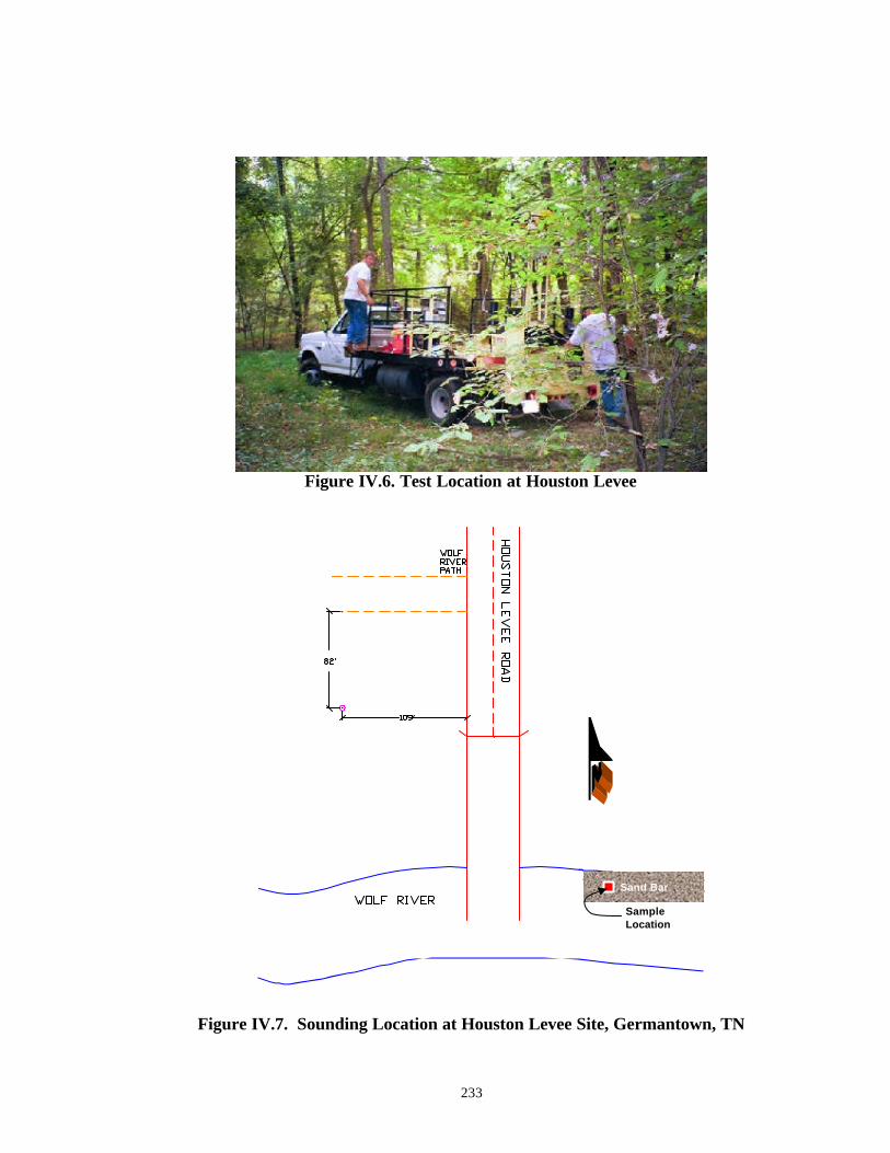
233
Figure IV.6. Test Location at Houston Levee
Figure IV.7. Sounding Location at Houston Levee Site, Germantown, TN
Sand Bar
SampleLocation

234
Figure IV.8. Test Site at Wolf River Boulevard Construction Site
Figure IV.9. Sounding Location at Wolf River Boulevard Site
N

235
property served as a bean field. Due to the dry weather, the surface crust of silt was
desiccated with a noticeable network of fissures. One sounding was performed near
where the property sloped down to the banks of the Wolf River.
IV.B.6 Monopole Tower
A site adjacent to a recently-drilled borehole became available in West Memphis, AR.
This provided an interesting opportunity to compare an interpreted CPT profile with soils
samples collected at approximately 1.5-meter intervals using SPT drive methods. Also,
this sounding was located in the floodplain west of the Mississippi River. This provided
an opportunity to compare soundings along the Wolf River to those just west of the
Mississippi River. Due to the dry weather, the surface crust of silt was desiccated with a
noticeable network of fissures. Figures 4.10 and 4.11 show the site and location of the
tests respectively.
IV.B.7 Shelby Forest
Shelby Forrest was a site set up by the USGS to compare shear wave
velocity measurements taken by a variety of different methods (personal communication
J. Gomberg, 1999). As opposed the other test sites in the Memphis area, this site was
located in the Pleistocene uplands (Bluffs) and near surface soils are not composed of
river deposits. This site was located Figures 4.12 and 4.13 show the test site and layout
of the soundings respectively.

236
Figure IV.10. Testing in West Memphis, AR
Figure IV.11. Test Locations at Monopole Tower, West Memphis, AR
N

237
Figure IV.12. Testing at Shelby Forest
Figure IV.13. Test Locations at Shelby Forrest,
N

238
IV.C Northeast Arkansas and Southeast Missouri
Fourteen soundings were performed at six test sites located in Northeast Arkansas
and Southeast Missouri, and one sounding was performed in Memphis, TN. Figure 4
shows the approximate locations of the sites in AR and MO with reference to pertinent
landmarks. Single soundings were performed at most locations, but multiple soundings
were performed to compare results of different penetrometers in similar soils and
evaluate soil conditions as distance from liquefaction features increased. Each test site
will be discussed in more detail in the following sub-sections.
IV.C.1 Yarbro Excavation
Yarbro (YARB) excavation is located between the Pemiscot Bayou and Arkansas
Route 150, north of Blytheville. Figures IV.15 and IV.16 show the test site and location
of the sounding respectively. The site is adjacent to a large sand excavation, which
shows evidence of a sand blow in the vicinity of the SCPTu sounding. The site has been
previously studied and dated by Tuttle and Schweig (1995) and Tuttle et al. (1996). The
liquefaction features appear to date from 1400-1600 and from 1811-1812.
IV.C.2 Bugg 40 (Haynes -307)
Bugg 40 (BUGG) is located off of Route 61, just south of the 150 Spur Split.
Figures IV.17 and IV.18 show the test site and layout of the soundings respectively.
Paleoliquefaction studies have been performed at this site, and are discussed in Tuttle et
al. (1998). Two soundings were performed. The first (BUGG-01) was adjacent to a
mapped liquefaction feature, and the second (BUGG-02) was located in an area of no
liquefaction features. These liquefaction features have been dated to occur between 800-

239
Figure IV.14. Location of Test Sites in Northeast AR and Southeast MO
Legend
Yarbro Excavation
Bugg 40
Dodd Farm
3MS617
Johnson Farm
Huey House
I-155 Bridge Steele
MISSOURI
ARKANSAS
TENNESSEE

240
Figure IV.15. Yarbro excavation test site
Figure IV.16. Test layout at Yarbro excavation test site
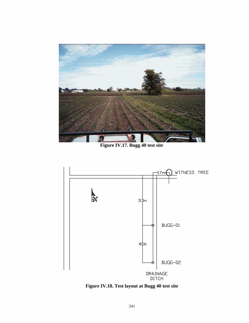
241
Figure IV.17. Bugg 40 test site
Figure IV.18. Test layout at Bugg 40 test site

242
1000 (Tuttle et al., 1998). Additional geophysical reconnaissance data is available at this
site, and has been presented in Wolf et al. (1998) and Collier (1998).
IV.C.3 3MS617 (Sigmund Site)
At the time of in-situ testing, an archeological dig and paleoliquefaction study were
underway. Figures IV.19 and IV.20 show the test site and layout of the soundings
respectively. Two trenches were being mapped, and surface artifacts were being
collected for dating purposes. Three soundings were performed close to an
approximately 1-meter wide sand blow. Dating of the site has not yet been completed,
but the liquefaction feature adjacent to the test locations is believed to be an 1811-1812
feature (Schweig, 1998).
IV.C.4 Huey House
The Huey House (HUEY) site is located on the south side of Route 150, north of
Blytheville, AR. Figure IV.21 shows the test layout and the anticipated location of the
paleoliquefaction study trench at this site. One sounding was performed at this site in the
general area of a mapped sand blow. Previous studies date the liquefaction feature from
between 880 and 1000 (Tuttle et al., 1998).
IV.C.5 Johnson Farm
Johnson farm (JOHN) is located north of Steel Missouri, along the Pemiscot
Bayou. Figure IV.22 shows the test layout and the location of 2 trenches from previous
paleoliquefaction studies. One sounding was performed at this site in the general area of a
mapped sand blow. Previous studies date the liquefaction feature from between 770 and
1200 (Tuttle et al., 1998).

243
Figure IV.19. 3MS617 test site
Figure IV.20. Test layout at 3MS617 site

244
Figure IV.21. Test layout at Huey House site
Figure IV.22. Test layout at Johnson farm site

245
IV.C.6 Dodd Farm
Dodd farm (DODD) is located north of Steel Missouri, and south of the Johnson site.
Figure IV.23 and IV.24 show the test site and layout of the soundings respectively. Three
CPTu soundings were performed at this site, and 3 DMT soundings were performed
adjacent to the CPTs at a later date. One of each test type (SCPTu, DODD-01; DMT,
DODD-06) was performed in the general area of a previous paleoliquefaction study
trench. A liquefaction feature is believed to have originated between 1400 and 1670
(Tuttle et al., 1998). Additional pairs of soundings were performed to analyze soil
conditions at increasing distance from the liquefaction feature. Geophysical surveys have
been performed at this site, and are reported in Collier (1998).
IV.C.7 I-155 Bridge
This bridge is a key lifeline facility. It is the only major bridge crossing the
Mississippi River between Memphis & St. Louis. A subsurface investigation and sesimic
retrofit were performed on the Tennessee side of the river in 1994 (Woodward Clyde,
1994). This study herein was concerned with soil properties on the Missouri Side of the
river. Seismic piezocones tests with pore pressure readings taken midface and behind the
tip were performed during this study. Flat dilatometer tests were also performed at this
site. Figure IV.25 displays the layout for testing performed at the I-155 bridge. Figure
IV.26 displays a close up of tests between the third and fourth column set and Figure
IV.27 is a photograph of the cone truck. Figure IV.28 displays a closeup of tests between
the fourth and fifth column set, and Figure IV.29 presents a photograph of the dilatometer
setup.
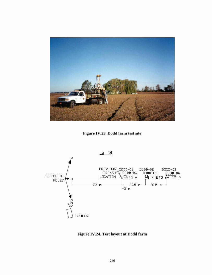
246
Figure IV.23. Dodd farm test site
Figure IV.24. Test layout at Dodd farm

247
Figure IV.25. Layout of all tests performed under the I-155 bridge

248
Figure IV.26. Detailed layout of tests between third and fourth column set
Figure IV.27. Photograph of GT GeoStar Truck set up under I-155 Bridge

249
Figure IV.28. Detailed layout of tests between fourth and fifth column set
Figure IV.29. Photograph of setup for Dilatometer Testing at I-155 Bridge

250
IV.D Charleston, S.C.
Soundings in Charleston, SC were performed at previously studied historic
liquefaction sites (Clough & Martin, 1990; Martin & Clough, 1994). Liquefaction at
these sites was expected to have occurred during the 1886 event, which had an epicenter
about 15 miles northwest of Charleston near Sommerville and Middleton Place (Martin,
1990). Two sites were investigated with seismic piezocones performed at each. Figure
4.30 displays approximate site locations with reference to Charleston. In addition,
Vibrocone soundings were performed at each site to test the feasibility of the initial
pneumatic impulse generator as a tool for liquefaction evaluation (Schneider et al., 1999).
Each test site will be described in more detail in the following subsections.
Figure IV.30. Location of Test Sites in the Charleston, S.C. Area (www.mapblast.com)
Legend Thompson Industrial Services Hollywood Ditch

251
IV.D.1 Hollywood Ditch
Hollywood Ditch (HW) was located in the town of Hollywood, SC and consisted
of a series of drainage ditches running east-west and north-south (Martin, 1990). The
section tested in this study was along an east-west trench, about 30 m east of State Rout
165. A soil boring (W-100) was located about 225 m west of S. R. 165, and a CPT
sounding (CPT 0+515) was located about 250 m east along the drainage ditch (Martin,
1990). Extensive liquefaction was observed along the sides of the drainage ditches in this
area as reported by Obermeir et al. (1986).
IV.D.2 Thompson Industrial Services
Thompson Industrial Services (TIS) is a site located between the prior studied
sites of Ten Mile Hill and Eleven Mile Post (Clough & Martin, 1990). The site consists
of an open field which was wooded until recently. Figure IV.33 displays a photograph of
the site, and Figure IV.34 presents a sounding layout map. While no surface evidence of
liquefaction was noticed at this site, no studies were performed at this location. The site
classifies as a non liquefy site, but it is located between two of the most severe areas of
liquefaction from the Charleston, SC 1886 event (Martin, 1990). For analysis purposes,
it is considered that liquefaction may have occurred in these soils.

252
Figure IV.31. Hollywood Ditch Site
Figure IV.32. Test layout at Hollywood Ditch test site

253
Figure IV.33. Thompson Industrial Services (TIS) Site
Figure IV.34. Test layout at TIS site

254
REFERENCES
Alarcon-Guzman, A., Leonards, G.A., and Chameau, J.L. (1988). Undrained monotonic and cyclic strength of sands, Journal of Geotechnical Engineering, 114 (10), ASCE, pp. 1089-1108. Ambraseys, N.N. (1988). Engineering seismology, Earthquake Engineering and Structural Dynamics, 17, pp. 1-105. Andrus, R.D., and Stokoe, K.H. (1997). Liquefaction resistance based on shear wave velocity, Proceedings, Workshop on Evaluation of Liquefaction Resistance, NCEER-97-0022, Multidisciplinary Center for Earthquake Engineering Research, Buffalo, NY, pp. 89-128. Andrus, R.D., Stokoe, K.H., and Chung, R.M. (1999). Draft guidelines for evaluating liquefaction resistance using shear wave velocity measurements and simplified procedures, NISTIR 6277, National Institute of Standards and Technology, Gaithersburg, MD, 121 pp. Arango, I. (1996). Magnitude scaling factors for soil liquefaction evaluation, Journal of Geotechnical Engineering, 122 (11), ASCE, pp. 929-936. Arango, I. (1997). Historical and continued role of the Standard Penetration Test method in geotechnical earthquake engineering, Proceedings, 3rd Seismic Short Course on Evaluation and Mitigation of Earthquake Induced Liquefaction Hazards, San Francisco, March 14. Arias, A. (1970). A measure of earthquake intensity, Seismic Design for Nuclear Power Plants, MIT Press, Cambridge, MA. Atkinson, G.M., and Boore, D.B. (1995). Ground-motion relations for eastern North America, Bulletin of the Seismological Society of America, 85, pp. 17-30. Atkinson, G.M., and Boore, D.B. (1997). Some comparisons between recent ground-motions relations, Seismological Research Letters, 68 (1), pp. 24-40. ASTM D422-63 (1999). Standard Test Method for Particle-Size Analysis of Soils, ASTM Section 4, Vol. 4.09 Soil and rock (1) D420-D4914.

255
ASTM D854-92 (1999). Standard Test Method for Specific Gravity of Soils, ASTM Section 4, Vol. 4.09 Soil and rock (1) D420-D4914. ASTM D1586-98 (1999). Standard Test Method for Penetration Testing and Spilt-Barrel Sampling of Soils, ASTM Section 4, Vol. 4.09 Soil and rock (1) D420-D4914. ASTM D4253-93 (1999). Standard Test Methods for Maximum Index Density and Unit Weight of Soils Using a Vibratory Table, ASTM Section 4, Vol. 4.09 Soil and rock (1) D420-D4914. ASTM D4254-91 (1999). Standard Test Method for Minimum Index and Unit Weight of Soils and Calculation of Relative Density, ASTM Section 4, Vol. 4.09 Soil and rock (1) D420-D4914. ASTM D4318-93 (1999). Standard Test Method for Liquid Limit, Plastic Limit, and Plasticity Index of Soils, ASTM Section 4, Vol. 4.09 Soil and rock (1) D420-D4914. ASTM D4633-85 (1999). Standard Method for Determination of Stress Wave Energy of Dynamic Penetrometer Systems, ASTM Section 4, Vol. 4.09 Soil and rock (1) D420-D4914. ASTM D5778-95 (1997). Standard Test Method for Performing Electronic Friction Cone and Piezocone Penetration testing of Soils, ASTM Section 4, Vol. 4.09 Soil and Rock (II). ASTM D6066-96 (1996). Standard Practice for Determining Normalized Penetration Resistance of Sands for Liquefaction Resistance Evaluation, ASTM Section 4, Vol. 4.09 Soil and Rock (II). Baldi, G., Bellotti, R., Ghionna, V.N., Jamiolkowski, M., and LoPresti, D.C.F. (1989). Modulus of sands from CPTs and DMTs, Proceedings of the Twelfth International Conference on Soil Mechanics and Foundation Engineering, Vol. 1, Rio de Janeiro, pp. 165-170. Baldwin, K.C., deAlba, P.A., and Jones, A.N. (1990). Relationship between acoustic and mechanical properties of two marine clays, Proceedings of the Conference on Shear Waves in Marine Sediments, Kluwer Academic Publishers, Dordrecht . pp. 95. Bates, C.R. (1989). Dynamic soil property measurements during triaxial testing, Geotechnique, 39(4), pp. 721-726. Bauer, B. (1999). Shear wave velocity of geologic formations of the Mississippi River Valley, personal communication to Bob Herrmann, Illinois Geologic Society.

256
Been, K. (1999). The critical state line and its application to soil liquefaction, Physics and Mechanics of Soil Liquefaction, Balkema, Rotterdam, pp. 195-204. Been, K., Crooks, J.H.A., Becker, D.E., and Jefferies, M.G. (1986). The cone penetration test in sands; part I, state parameter interpretations, Geotechnique, 36, pp. 239-249. Been, K., and Jefferies, M.G. (1985). A state parameter for sands, Geotechnique, 35 (2), pp. 99-112. Been, K., Jefferies, M.G., Crooks, J.H.A., and Rothenburg, L. (1987). The cone penetration test in sands: part II, general inference of state, Geotechnique, 37, pp. 285-299. Been, K., Jefferies, M.G., and Hachey, J. (1991). The critical state of sands, Geotechnique, 41 (3), pp. 365-381. Berry, K.M., Olson, S.M., and Lamie, M. (1998). Cone penetration testing in the Mid-Mississippi River Valley, Geotechnical Site Characterization, Vol. 2, Balkema, Rotterdam, pp. 983-987. Bollinger, G.A. (1983). Speculation on the nature of seismicity at Charleston, South Carolina, Studies Related to the Charleston, South Carolina, Earthquake of 1886 - Tectonics and Seismicity, U.S. Geologic Survey Professional Paper 1313, pp. T1-T11. Bollinger, G.A. (1977). Reinterpretation of the intensity data for the 1886 Charleston, South Carolina earthquake, Studies Related to the Charleston, South Carolina, Earthquake of 1886, A Preliminary Report, U.S. Geologic Survey Professional Paper 1028, pp. 17-32. Boore, D.B. (1996). SMSIM - Fortran program for simulating ground motions from earthquakes: version 1.0, USGS Open File Report 96-80-A. Boore, D.B., and Joyner, W.B. (1991). Estimation of ground motion at deep soil sites in eastern North America, Bulletin of the Seismological Society of America, 81(6), pp. 2167-2185. Boulanger, R.W., Mejia, L.H., and Idriss, I.M. (1997). Liquefaction at Moss Landing during the Loma Prieta earthquake, Journal of Geotechnical and Geoenvironmental Engineering, 123 (5), ASCE, pp. 453-467. Broms, B.B., and Flodin, N. (1988). History of soil penetration testing, Penetration Testing 1988, ISOPT-1, Balkema, Rotterdam, pp. 157-220.

257
BS 1377 (1990)., Standard test method for Fall Cone method, British Standards, Part 1 & 2. Campanella, R.G. (1994). Field methods for dynamic geotechnical testing: an overview of capabilities and needs, Dynamic Geotechnical Testing II, ASTM STP 1213, Philadelphia, pp. 3-23. Campanella, R.G., Gillespie, D., and Robertson, P.K. (1982). Pore pressures during cone penetration, Proceedings 2nd European Symposium on Penetration Testing, Vol. 2, Amsterdam, pp. 507-512. Campanella, R.G., and Robertson, P.K. (1988). Current status of the piezocone test, Penetration Testing 1988, Balkema, Rotterdam, pp. 93-116. Campanella, R.G., Robertson, P.K., and Gillespie, D. (1986). Seismic cones penetration tests, Use of In-Situ Tests in Geotechnical Engineering, ASCE GSP 6, pp. 116-130. Casagrande, A. (1936). Characteristics of cohesionless soils affecting the stability of slopes and earth fills, Contributions to Soil Mechanics, Boston Society of Civil Engineers, 1940, pp. 257 - 276. Castro, G. (1969). Liquefaction of sands, Harvard Soil Mechanics Series 87, Harvard University, Cambridge, Massachusetts. Chang, F.K., and Krinitzsky, E.L. (1977). Duration, spectral content, and predominant period of strong motion earthquake records from western United States, Miscellaneous Paper 5-73-1, U.S. Army Corps of Engineers Waterways Experiment Station, Vicksburg. Chen, B.S., and Mayne, P.W. (1994). Profiling the overconsolidation ratio of clays by piezocone tests, Report No. GIT-CEEGEO-94-1, School of Civil and Environmental Engineering, Georgia Institute of Technology, Atlanta, GA, 279 pp. Chameau, J.-L., A., Clough, G.W., Frost, J.D., and Reyna, F.A.M. (1998). Liquefaction characteristics of the San Francisco bayshore fills, The Loma Prieta Earthquake of October17, 1989 – Liquefaction, United States Geologic Survey Professional Paper 1551-B, pp. 9-24. Clough, G.W., and Martin, J.R., II. (1990). Geotechnical setting for liquefaction events in the Charleston, South Carolina Vicinity, Proceedings H.B. Seed Memorial Symposium, Vol. 2, BiTech Publishers, Vancouver, B.C. Collier, J.W. (1998). Geophysical Investigations of Liquefaction Features in the New Madrid Seismic Zone: Northeastern Arkansas and Southeastern Missouri, M.S. Thesis, Auburn University, Auburn, AL, 163 pp.

258
Cunning, J.C., Robertson, P.K., and Sego, D.C. (1995). Shear wave velocity to evaluate in-situ state of cohesionless soils, Canadian Geotechnical Journal, 32, pp. 848-858. Darendeli, M.B., (1997). Dynamic properties of soils subjected to 1994 Northridge earthquake, MS Thesis, School of Civil Engineering, The University of Texas at Austin, Austin, TX, 605 pp. Decourt, L., Muromachi, T., Nixon, I.K., Schmertmann, J.H., Thorburn, S., and Zolkov, E. (1988). Standard penetration test (SPT): International reference test procedure, Penetration Testing 1988, ISOPT-1, Vol. 1, Balkema, Rotterdam, pp. 3-26. Desrues, J., Chambon, R., Mokni, M., and Mazerolle, F. (1996). Void ratio evolution inside shear bands in triaxial sand specimens studied by computed tomography, Geotechnique, 46 (3), pp. 123-132. Dobry, R., Elgamal, A.-W., and Bazair, M. (1989). Pore pressure and acceleration response of Wildlife site during the 1987 Earthquake, Proceedings from the Second U.S.-Japan Workshop on Liquefaction, Large Ground Deformation and their Effects on Lifelines, NCEER-89-0032, Multidisciplinary Center for Earthquake Engineering Research, Buffalo, NY, pp. 145-160. Dobry, R., Ladd, R.S., Yokel, F.Y., Chung, R.M., and Powell, D. (1982). Prediction of pore water pressure buildup and liquefaction of sands during earthquakes by the cyclic strain method, NBS Building Science Series 138, National Bureau of Standards, Gaithersburg, MD, 150 pp. Douglas, B.J., and Olsen, R.S. (1981). Soil classification using electric cone penetrometers, Cone Penetration Testing and Experience, ASCE, pp. 209-227. Dutton, C.E. (1889). The Charleston earthquake of August 31, 1886, U.S. Geologic Survey Annual Report, 1887-1888, pp. 203-528. Elgamal, A.-W., Zeghal, M., Parra, E., Gunturi, R., Tang, H.Y., and Stepp, J.C. (1996). Identification and modeling of earthquake ground response - I. Site amplification, Soil Dynamics and Earthquake Engineering, 15, pp. 499-522. Fam, M., and Santamarina, J.C. (1997). A study of consolidation using mechanical and electromagnetic waves, Geotechnique, 47 (2), pp. 203 - 219. Farrar, J.A. (1998). Summary of Standard Penetration Test (SPT) energy measurement experience, Geotechnical Site Characterization, Vol. 2, Balkema, Rotterdam, pp. 919-926.

259
Fear, C.E., and Robertson, P.K. (1995). Estimation of the undrained shear strength of sand: a theoretical framework, Canadian Geotechnical Journal, 32, pp. 859-870. Finn, W.D.L., Lee, K.W., and Martin, G.R. (1977). An effective stress based model for liquefaction, Journal of Geotechnical Engineering Division, ASCE, 103 (GT6), pp. 517-533. Frankel, A., Mueller, C., Barnhard, T., Perkins, D., Leyendecker, E.V., Dickman, N., Hanson, S., and Hopper, M. (1996). National Seismic-Hazard Maps: Documentation June 1996, USGS Open-File report 96-532. Frost, J.D., Chameau, J.-L.A., Reyna, F.A.M., and Karanikolas, P. (1993). Performance of fill soils during the Loma Prieta earthquake, Proceedings, Third International Conference on Case Histories in Geotechnical Engineering, Vol. 3, St. Louis, pp. 541-546. Frost, J.D., Chen, C.-C., Park, J.-Y., and Jang, D.-J. (1999). Quantitative characterization of microstructure evolution, Physics and Mechanics of Soil Liquefaction, Balkema, Rotterdam, pp. 169 - 177. Garcia, S. R. (1991). Interrelationship Between the Initial Liftoff and Extended Pressure Readings of the Marchetti Flat Blade Dilatometer in Soils, M.S. Thesis, Georgia Institute of Technology, Atlanta, GA, 119 pp. Gohn, G.S., Houser, B.B., and Schneider, R.R. (1983). Geology of the lower mesozoic sedimentary rocks in Clubhouse Crossroads test hole #3, near Charleston, South Carolina, Studies Related to the Charleston, South Carolina, Earthquake of 1886 - Tectonics and Seismicity, U.S. Geologic Survey Professional Paper 1313, pp. D1-D17. Green, R.K., Cooling, T.L., Mejia, L.H., and Abrahamson, N.A. (1995). Earthquake motions and seismic evaluation of Cape Girardeau bridge, Lifeline Earthquake Engineering, ASCE, pp. 517-524. Gutenberg, B., and Richter, C.F. (1956). Magnitude and energy of earthquakes, Annali di Geofisica, 9 (1), pp. 2825-2852. Hardin, B.O., and Drnevich, V.P. (1972). Shear modulus and damping in soils: design equations and curves, Journal of the Soil Mechnaics and Foundation Division, 94(2), ASCE, pp. 353-368. Hegazy, Y.A., and Mayne, P.W. (1995). Statistical correlations between shear wave velocity and cone penetration data for different soil types, Proceedings, International Symposium on Cone Penetration Testing (CPT '95), Vol. 2, Swedish Geotechnical Society Report No. 3:95, Linkoping, pp. 173-178.

260
Herrmann, R.B. (1999). Personal Communication, April (Department of Earth and Atmospheric Sciences, St. Louis University, St. Louis, MO). Herrmann, R.B., and Akinci, A. (1999). Mid-America Ground Motion Models, http://www.eas.slu.edu/People/RBHerrmann/MAEC/maecgnd.html, Department of Earth and Atmospheric Sciences, Saint Louis University, St. Louis, MO, 63103, 8 pp. Herrmann, R.B., Ortega, R., and Akinci, A. (1999). Mid-America probabilistic hazard maps, http://www.eas.slu.edu/People/RBHerrmann/HAZMAP/hazmap.html , Department of Earth and Atmospheric Sciences, Saint Louis University, St. Louis, MO, 63103, 5 pp. Holzer, T.L., Youd, T.L., and Hanks, T.C. (1989). Dynamics of liquefaction during the 1987 Superstition Hills, California, earthquake, Science, 244, pp. 56-59. Hoyos, L.R. Jr., Sheppard, B., Shao, Y., and Macari, E.J. (1999). Results of resonant column testing program performed on sands from Memphis, TN, and West Memphis, AR, Interim Report, MAEC Project No. GT-1, Dynamic Properties of Mid-American Soils, April, pp. 17. Hryciw, R.D., and Thomann, T.G. (1993). Stress-history-based model for Ge of cohesionless soils, Journal of Geotechnical Engineering, 119 (7), ASCE, pp. 1073-1093. Idriss, I.M. (1985). Evaluating seismic risk in engineering practice, , 11th International Conference on Soil Mechanics and Foundation Engineering, Vol. 1, Balkema, Rotterdam, pp. 255-320. Idriss, I.M. (1991). Response of soft sites during earthquake, H. Bolton Seed Memorial Symposium, Vol. 2, BiTech Publishers, Ltd., Vancouver, pp. 273-289. Idriss, I.M. (1999). An update of the Seed-Idriss simplified procedure for evaluating liquefaction potential, Presentation Notes, Transportation Research Board '99 Workshop on New Approaches to Liquefaction Analysis, Washington D.C., January 10, 21 pp. Idriss, I.M., Lysmer, J., Hwang, R., and Seed, H.B. (1973). QUAD4 – A computer program for evaluating the seismic response of soil structures by variable damping finite element procedures, Report No. EERC 73-16, Earthquake Engineering Research Center, University of California, Berkeley, CA, 67 pp. Idriss, I.M., and Sun, J.I. (1992). User's manual for SHAKE91, A computer program for conducting equivalent linear seismic response analysis of horizontally layered soil deposits, Center for Geotechnical Modeling, Department of Civil & Environmental Engineering, University of California, Davis, August.

261
Indridason, J.K. (1992). Strain based evaluation of liquefaction during the 1886 Charleston earthquake, Research Project, School of Civil and Environmental Engineering, Georgia Institute of technology, Atlanta, GA, 158 pp. Ishibashi, I. (1992). Discussion to, Effect of soil plasticity on cyclic response, Journal of Geotechnical Engineering, 118 (5), ASCE, pp. 830-832. Ishihara, K. (1985). Stability of natural deposits during earthquakes, Proceedings, 11th International Conference on Soil Mechanics and Foundation Engineering, Vol. 1, Balkema, Rotterdam, pp. 321-376. Ishihara, K. (1993). Liquefaction and flow failures during earthquakes, Geotechnique, 43 (3), pp. 351-415. Ishihara, K., Anazawa, Y., and Kuwano, J. (1987). Pore water pressures and ground motions monitored during the 1985 Chiba-Ibaragi earthquake, Soils and Foundations, 27 (3), pp. 13-30. Ishihara, K., Shimizu, K., and Yamada, Y. (1981). Pore water pressures measured in sand deposits during an earthquake, Soils and Foundations, 21 (4), pp. 85-100. Jamiolkowski, M., Baldi, G., Bellotti, R., Ghionna, V., and Pasqualini, E. (1985a). Penetration resistance and liquefaction of sands, Proceedings Eleventh International Conference on Soil Mechanics and Foundation Engineering, Vol. 4, Balkema, Rotterdam, pp. 1891-1896. Jamiolkowski, M., Ladd, C.C., Germaine J.T., and Lancellotta, R. (1985b). New developments in field and laboratory testing of soils, Proceedings Eleventh International Conference on Soil Mechanics and Foundation Engineering, Vol. 1, Balkema, Rotterdam, pp. 57-153. Jefferies, M.G. (1999). A critical view of liquefaction, Physics and Mechanics of Soil Liquefaction, Balkema, Rotterdam, pp. 221-235. Johnston, A.C., and Schweig, E.S. (1996). The enigma of the New Madrid earthquakes of 1811-1812, Annual Review of Earth and Planetary Sciences, 24, pp. 339-384. Jones, G., and Rust, E. (1982). Piezometer penetration testing, Proceedings 2nd European Symposium on Penetration Testing, Vol. 2, Amsterdam, pp. 607-613. Kavazanjian, E. (1999). Personal Communication, January (GeoSyntec, Hunnington Beach, CA).

262
Kayen, R.E., and Mitchell, J.K. (1997). Assessment of liquefaction potential during earthquakes by Arias intensity, Journal of Geotechnical and Geoenvironmental Engineering, ASCE, 123 (12), pp. 1162-1174. Kayen, R.E., Mitchell, J.K., Seed, R.B., Lodge, A., Nishio, S., and Coutinho, R. (1992). Evaluation of SPT, CPT, and shear wave velocity based methods for liquefaction potential assessment using Loma Prieta data, Proceedings 4th Japan-U.S. Workshop on Earthquake Resistance Design of Lifeline Facilities and Countermeasures for Soil Liquefaction, NCEER-92-0019, Buffalo, NY, pp. 177-192. Keane, C.M., and Prevost, J.H. (1989). An analysis of earthquake data observed at the Wildlife liquefaction array site, Imperial County, California, Proceedings from the Second U.S.-Japan Workshop on Liquefaction, Large Ground Deformation and their Effects on Lifelines, NCEER-89-0032, Multidisciplinary Center for Earthquake Engineering Research, Buffalo, NY, pp. 176-192. Konrad, J.M. (1988). Interpretation of Flat Plate Dilatometer Tests in Sands in Terms of the State Parameter, Geotechnique, 38 (2), pp. 263-277. Kramer, S.L. (1996). Geotechnical Earthquake Engineering, Prentice Hall, Upper Saddle River, NJ, 653 pp. Kulhawy, F.H., and Mayne, P.W. (1990). Manual on estimating soil properties for foundation design, Report EL-6800, Electric Power Research Institute, Palo Alta, CA, August, 306 pp. Kuo, C.-Y., and Frost, J.D. (1997). Initial fabric and uniformity of a sand specimen - an image analysis approach, Mechanics of Deformations and Flow of Particulate Materials, ASME-ASCE-SUS Joint Summer Meeting, pp. 214-227. Ladd, R.S., Dobry, R., Dutko, P., Yokel, F.Y., and Chung, R.M. (1989). Pore-water pressure buildup in clean sands because of cyclic straining, Geotechnical Testing Journal, 12 (1), ASTM, pp. 77-86. Lambe, T.W., and Whitman, R.V. (1969). Soil Mechanics, John Wiley & Sons, New York, 553 pp. Lee, K.L., and Seed, H.B. (1967). Drained strength characteristics of sands, Journal of the Soil Mechanics and Foundation Division, 93 (SM6)., ASCE, pp. 117-141. Lee, M.K.W., and Finn, W.D.L. (1978). DESRA-2: Dynamic effective stress response analysis of soil deposits with energy transmitting boundary including assessment of liquefaction potential, Soil Mechanics Series No. 38, Department of Civil Engineering, University of British Columbia, Vancouver, June, 57 pp.
263
Liao, S.S.C., and Whitman, R.V. (1986). Overburden correction factors for SPT in sand, Journal of Geotechnical Engineering, 112 (3), ASCE, pp. 373-377. Liu, H.-P., Hu, Y., Dorman, J., Chang, T.-S., and Chiu, J.-M. (1997). Upper Mississippi embayment shallow seismic velocities measured in situ, Engineering Geology, 46, pp. 313-330. Lunne, T., Eidsmoen, T., Gillespie, D., and Howland, J.D. (1986). Laboratory and field evaluation of cone penetrometers, Use of In-Situ Tests in Geotechnical Engineering, ASCE GSP 6, pp. 714-729. Lunne, T., Robertson, P.K., Powell, J.J.M. (1997). Cone Penetration Testing in Geotechnical Practice, Blackie Academic & Professional, New York, 312 pp. Marchetti, S. (1980). In-Situ Tests by Flat Dilatometer, Journal of Geotechnical Engineering, 106 (GT3), pp. 299-321. Martin, J.R. (1990). Implications from a geotechnical investigation of liquefaction phenomena associated with seismic events in the Charleston, SC area, Ph.D. Thesis, School of Civil Engineering, Virginia Polytechnic and State University, Blacksburg, VA, 414 pp. Martin, J.R. II., and Clough, G.W. (1994). Seismic parameters from liquefaction evidence, Journal of Geotechnical Engineering, 120 (8), ASCE, pp. 1345-1361. Masood, T., and Mitchell, J.K. (1993). Estimation of in-situ lateral stresses in soil by cone penetration tests, Journal of Geotechnical Engineering, 119 (10), ASCE, pp. 1624-1639. Mayne, P.W. (1991). Tentative method for estimating σho' from qc data in sands, Calibration Chamber Testing, ISSOCT-1, Elsevier, New York, pp. 249-256. Mayne, P.W. (1995). CPT determination of overconsolidation ratio and lateral stresses in clean quartz sands, Proceedings, International Symposium on Cone Penetration Testing (CPT '95), Vol. 2, Swedish Geotechnical Society Report No. 3:95, Linkoping, pp. 215-220. Mayne, P.W., and Kulhawy, F.H. (1982). Ko - OCR relationships in soil, Journal of Geotechnical Engineering Division, 108 (GT6), pp. 851-872. Mayne, P.W., and Kulhawy, F.H. (1991). Calibration chamber database and boundary effects correction for CPT data, Calibration Chamber Testing, Elsevier, New York, pp. 257-264.

264
Mayne, P.W., Kulhawy, F.H., and Kay, J.N. (1990). Observations on the development of pore-water stresses during piezocone penetration in clays, Canadian Geotechnical Journal, 27 (4), pp. 418-428. Mayne, P.W., Mitchell, J.K., Auxt, J.A., and Yilmaz, R. (1995). U.S. National Report on CPT, Proceedings, International Symposium on Cone Penetration Testing (CPT '95), Vol. 1, Swedish Geotechnical Society Report No. 3:95, Linkoping, pp. 263-276. Mayne, P.W., and Rix, G.J. (1993). Gmax - qc relationships for clays, Geotechnical Testing Journal, 16 (1), ASTM, pp. 54-60. Mayne, P.W., and Rix, G.J. (1995). Correlations between shear wave velocity and cone tip resistance in natural clays, Soils and Foundations, 35 (2), pp. 107-110. Mayne, P.W., Schneider, J.A., and Martin, G.K. (1999). Small- and large-strain soils properties from seismic flat dilatometer tests, Proceeding, Pre-failure deformation characteristics of geomaterials, Torino '99, Balkema, Rotterdam, 8 pp. Mitchell, J.K., and Brandon, T.L. (1998). Analysis and use of CPT in earthquake and environmental engineering, Geotechnical Site Characterization, Vol. 1, Balkema, Rotterdam, pp. 69-97. NCEER (1997). Summary report, Proceedings, Workshop on Evaluation of Liquefaction Resistance, NCEER-97-0022, Multidisciplinary Center for Earthquake Engineering Research, Buffalo, NY, pp. 1-40. Newmark, N.M., and Hall, W.J. (1982). Earthquake spectra and design, EERI Monograph, Earthquake Engineering Research Institute, Berkeley, CA, 103 pp. Norton, W.E. (1983). In-situ determination of liquefaction potential using the PQS probe, Technical Report GL-83-1, U.S. Army Corps of Engineers, Waterways Experiment Station, Vicksburg, MS, 101 pp. Nuttli, O.W., and Brill, K.G. Jr. (1981). 1981, Catalog of central United States earthquakes since 1800 of mb > 3.0, Part II and Appendix B-2: in Barstow, N.L., K.G. Brill Jr., O.W. Nuttli and P.W. Pomeroy, An Approach to Seismic Zonation for Siting Nuclear Electric Power Generating Facilities in the Eastern United States, NUREG/CR-1577, U.S. Nuclear Regulatory Commission, Washington, D.C., p. 97-143, B2-1-B2-31, 4 plates (#411). Nuttli, O.W., and Herrmann, R.B. (1984). Ground motion of Mississippi Valley earthquakes, Journal of Technical Topics in Civil Engineering, 110 (1), ASCE, pp. 54-69.

265
Obermeier, S.F., Jacobson, R.B., Powars, D.S., Weems, R.E., Hallbick, D.C., Gohn, G.S., and Markewich, H.W. (1986). Holocene and late Pleistocene earthquake-induced sand blows in coastal South Carolina, Proceedings, 3rd U.S. National Earthquake Engineering Conference, Charleston, S.C, pp. 197-208. Olsen, R.S. (1984). Liquefaction analyses using the cone penetration test, Proceedings of the 8th World Conference of Earthquake Engineering, Vol. 3, pp. 247-254. Olsen, R.S. (1988). Using the CPT for dynamic site response characterization, Earthquake Engineering and Soil Dynamics II, ASCE GSP 21, pp. 374-388. Olsen, R.S. (1994). Normalization and prediction of geotechnical properties using the cone penetration test (CPT), Technical Report GL-94-29, U.S. Army Corps of Engineers, Vicksburg, August, 292 pp. Olsen, R.S. (1997). Cyclic liquefaction based on the cone penetrometer test, Proceedings, Workshop on Evaluation of Liquefaction Resistance, NCEER-97-0022, Multidisciplinary Center for Earthquake Engineering Research, Buffalo, NY, pp. 225-276. Olsen, R.S., and Mitchell, J.K. (1995). CPT stress normalization and prediction of soil classification, Proceedings, International Symposium on Cone Penetration Testing (CPT '95), Vol. 2, Swedish Geotechnical Society Report No. 3:95, Linkoping, pp. Olson, S.M. (1997). Liquefaction shear strength of granular soils, Preliminary Proceedings of the Workshop: Post-Liquefaction Shear Strength of Granular Soils, NSF CMS-95-31678, Urbana, Illinois, pp. 123-146. Olson, S.M., and Stark, T.D. (1998). CPT based liquefaction resistance of sandy soils, Geotechnical Earthquake Engineering and Soil Dynamics III, ASCE GSP 75, pp. 325-336. Pond, E. C. (1996). Seismic parameters for the central United States based on paleoliquefaction evidence in the Wabash Valley, Ph.D. Thesis, School of Civil and Environmental Engineering, Virginia Polytechnic and State University. Poulos, S.J. (1981). The steady state of deformations, Journal of the Geotechnical Engineering Division, 107 (GT5), ASCE, pp. 553-562. Poulos, S.J., Castro, G., and France, J.W., (1985). Liquefaction evaluation procedure, Journal of Geotechnical Engineering, 111 (6), ASCE, pp. 772-792. Reyna, F., and Chameau, J.L. (1991). Dilatometer based liquefaction potential of sites in the Imperial Valley, Proceedings, Second International Conference on Recent Advances

266
in Geotechnical Earthquake Engineering and Soil Dynamics, Vol. 1, St. Louis, pp. 385-392. Risk Engineering (1994). Seismic hazard evaluation and multiple-support artificial ground motions for the A-1700 bridge, Pemiscot County, Missouri, Dyer County, Tennessee, Report, prepared for Sverdrup Civil Inc., Maryland Heights, Missouri, 63043, 146 pp. Rix, G.J., and Stokoe, K.H. (1991). Correlation of initial tangent modulus and cone penetration resistance, Calibration Chamber Testing, ISSOCT-1, Elsevier, New York, pp. 351-362. Robertson, P.K. (1990). Soil classification using the cone penetration test, Canadian Geotechnical Journal, 27 (1), pp. 151-158. Robertson, P.K., and Campanella, R.G. (1983). Interpretation of cone penetrometer test: Part I: Sand, Canadian Geotechnical Journal, 20 (4), pp. 718-733. Robertson, P.K., and Campanella, R.G. (1983). Interpretation of cone penetrometer test: Part II: Clay, Canadian Geotechnical Journal, 20 (4), pp. 734-745. Robertson, P.K., and Campanella, R.G. (1985). Liquefaction potential of sands using the CPT, Journal of Geotechnical Engineering, 111 (3), ASCE, pp. 384-403. Robertson, P.K., Campanella, R.G., Gillespie, D., and Greig, J. (1986). Use of piezomenter cone data, Use of In-Situ Tests in Geotechnical Engineering, ASCE GSP 6, pp. 1263-1280. Robertson, P.K., Sasitharan, S., Cunning, J.C., and Sego, D.C. (1995). Shear-wave velocity to evaluate in-situ state of Ottawa sand, Journal of Geotechnical Engineering, 121 (3), ASCE, pp. 262-273. Robertson, P.K., Woeller, D.J., and Finn, W.D.L. (1992a). Seismic cone penetration test for evaluating liquefaction potential under cyclic loading, Canadian Geotechnical Journal, 29, pp. 686-695. Robertson, P.K., Woeller, D.J., Kokan, M., Hunter, J., and Luternaur, J. (1992b). Seismic techniques to evaluate liquefaction potential, 45th Canadian Geotechnical Conference, Toronto, Ontario, October 26-28, pp. 5:1-5:9. Robertson, P.K., and Wride (Fear), C.E. (1997). Cyclic liquefaction and its evaluation based on the SPT and CPT, Proceedings, Workshop on Evaluation of Liquefaction Resistance, NCEER-97-0022, Multidisciplinary Center for Earthquake Engineering Research, Buffalo, NY, pp. 41-88.

267
Robertson, P.K., and Wride, C.E. (1998). Evaluating cyclic liquefaction potential using the cone penetration test, Canadian Geotechnical Journal, 35 (3), pp. 442-459. Rowe, P.W. (1964). The stress dilatency relations for static equilibrium of an assembly of particles in contact, Proceedings, Royal Society, London, Series A, Vol. 269, pp. 500-527. Roy, D., Campanella, R.G., Byrne, P.M., and Hughes, J.M.O. (1997). Strain level and uncertainty of liquefaction related index tests, Uncertainty in the Geologic Environment: From Theory to Practice, Vol. 2, GSP 58, ASCE, New York, pp. 1149-1162. Samiezade-Yazd, M., Herrmann, R.B., Malagnini, L., and Liu, W. (1999). A regional comparison of vertical ground motion in North America, http://www.eas.slu.edu/People/RBHerrmann/GroundMotion/ , Department of Earth and Atmospheric Sciences, Saint Louis University, St. Louis, MO, 63103, 37 pp. Santamarina, J.C., Fam, M.A., and Klein, K. (1999). Particulate Materials: Characterization with Elastic and Electromagnetic Waves, John Wiley & Sons, under contract. Sata, K., Kokusho, T., Matsumoto, M., and Yamada, E. (1996). Nonlinear seismic response and soil property during strong motion, Soils and Foundations Special Issue on the 1995 Hyogoken-Nambu Earthquake, January, pp. 41-52 Saucier, R.T. (1994). Geomorphology and Quaternary Geologic History of the Lower Mississippi Valley, U.S. Army Corps of Engineers Waterways Experiment Station, Vicksburg. Schofield, A.N., and Wroth, C.P. (1968). Critical State Soil Mechanics, McGraw-Hill, London. Schmertmann, J.H. (1986). Suggested Method for Performing the Flat Dilatometer Test, ASTM Geotechnical Testing Journal, 9 (2), pp. 93-101. Schneider, J.A., and Mayne, P.W. (1998a). “Results of Seismic Piezocone Penetration Tests Performed in Memphis, TN and West Memphis, AR,” Interim Report, MAEC Project No. GT-3, November, pp. 67. Schneider, J.A., and Mayne, P.W. (1998b). “Results of Seismic Piezocone and Flat Dilatometer Tests Performed in Blytheville, AR, Steele, MO, and Shelby County, TN Interim Report, MAEC Project No. GT-3, December, pp. 125.

268
Schneider, J.A., Mayne, P.W., Hendren, T.L., and Wise, C.M. (1999). Initial development of an impulse piezovibrocone for liquefaction evaluation, Physics and Mechanics of Soil Liquefaction, Balkema, Rotterdam, pp. 341-354. Schweig, E.S. (1998). Personal Communication, October, (CERI - Memphis). Schweig, E.S., and VanArsdale, R.B. (1996). Neotectonics of the upper Mississippi embayment, Engineering Geology, 45, pp. 185-203. Schnabel, P.B., Lysmer, J., and Seed, H.B. (1972). SHAKE: a computer program for earthquake response analysis of horizontally layered sites, Report EERC 72-12, Earthquake Engineering Research Center, University of California, Berkeley. Seed, H.B. (1979). Soil liquefaction and cyclic mobility evaluation for level ground during earthquakes, Journal of the Geotechnical Engineering Division, 105 (GT2), ASCE, pp. 201-255. Seed, H.B., and DeAlba, P. (1986). Use of SPT and CPT tests for evaluation of the liquefaction resistance of soils, Use of In-Situ Tests in Geotechnical Engineering, ASCE GSP 6, pp. 281-302. Seed, H.B., and Idriss, I.M. (1970). Soil moduli and damping factors for dynamic response analysis, Report No. EERC 70-10, Earthquake Engineering Research Center, University of California, Berkeley, reprinted in H. Bolton Seed Selected Papers, Vol. 1, BiTech Publishers, Ltd., Vancouver, pp. 277-308. Seed, H.B., and Idriss, I.M. (1971). Simplified procedure for evaluating soil liquefaction potential, Journal of Soil Mechanics and Foundation Division, ASCE, 97 (SM9), pp. 1249-1273. Seed, H.B., Idriss, I.M., and Arango, I. (1983). Evaluation of liquefaction potential from field performance data, Journal of Geotechnical Engineering, ASCE, 109 (3), pp. 458-482. Seed, H.B., Idriss, I.M., Makdisi, F., and Banerjee, N. (1975). Representation of irregular stress time histories by equivalent uniform stress series in liquefaction analysis, EERC 75-29, Earthquake Engineering Research Center, University of California, Berkeley. Seed, H.B., and Lee, K.L. (1966). Liquefaction of saturated sands during cyclic loading, Journal of Soil Mechanics and Foundation Division, ASCE, 92 (SM6), pp. 105-134. Seed, H.B., Tokimatsu, K., Harder, L.F., and Chung, R.M. (1985). Influence of SPT procedures in soil liquefaction resistance evaluations, Journal of Geotechnical Engineering, ASCE, 111 (12), pp. 1425-1445.

269
Seed, R.B., and Harder, L.F. (1990). SPT-based analysis of cyclic pore pressure generation and undrained residual strength, H. Bolton Seed Memorial Symposium, Vol. 2, BiTech Publishers, Vancouver, pp. 351-376. Sego, D.C., Hofmann, B.A., Robertson, P.K., and Wride, C.E. (1999). Undisturbed sampling of loose sand using in-situ ground freezing, Physics and Mechanics of Soil Liquefaction, Balkema, Rotterdam, pp. 179-191. Senneset, K., and Janbu, N. (1985). Shear strength parameters obtained from static CPT, Strength Testing of Marine Sediments, ASTM STP 883, Philadelphia, pp. 41-54. Senneset, K., Janbu, N., and Svano, G. (1982). Strength and deformation parameters from cone penetration tests, Proceedings 2nd European Symposium on Penetration Testing, Vol. 2, Amsterdam, pp. 863-870. Shen, C.K., Wang, Z., and Li, X.S. (1991). Pore pressure response during 1986 Lotung earthquakes, Proceedings, Second International Conference on Recent Advances in Geotechnical Earthquake Engineering and Soil Dynamics, March 11-15, 1991, St. Louis, Missouri, pp. 557-563. Shibata, T., Oka, F., and Ozawa, Y. (1996). Characteristics of ground deformations due to liquefaction, Soils and Foundations Special Issue on the 1995 Hyogoken-Nambu Earthquake, January, pp. 65-79. Shibata, T., and Teparaksa, W. (1988). Evaluation of liquefaction potential of soils using cone penetration tests, Soils and Foundations, 28 (2), pp. 49-60. Shibuya, S., Nakajima, M., Hosona, T. (1994). Pseudo elastic shear modulus of a Holocene clay deposit, Proceedings of the International Symposium on Pre-Failure Deformation Characteristics of Geomaterials, Vol. 1, pp. 293. Shuttle, D., and Jeffereis, M. (1998). Dimensionless and unbiased CPT interpretation in sand, International Journal for Numerical and Analytical Methods in Geomechanics, 22, pp. 351-391. Skempton, A.W. (1986). Standard penetration test procedures and the effects of overburden pressure, relative density, particle size, ageing, and overconsolidation, Geotechnique, 36 (3), pp. 425-447. Sladen, J.A. (1989). Problems with interpretation of sand state from cone penetration tests, Geotechnique, 39, pp. 323-332.

270
Stark, T.D., and Mesri, G. (1992). Undrained shear strength of liquefied sands for stability analysis, Journal of Geotechnical Engineering, 118 (11), ASCE, pp. 1727-1747. Stark, T.D., and Olson, S.M. (1995). Liquefaction resistance using CPT and field case histories, Journal of Geotechnical Engineering, 121 (12), pp. 859-869. Stokoe, K.H.,II, Darendeli, M.B., and Menq, F.-Y. (1999). Rosrine Project: Phases I and II, Summary of RC/TS laboratory test results, Lecture notes from, Symposium on Site Response Issues, MIT, Boston, March 19, 125 pp. Stover, and Coffman (1993). Seismicity of the United States 1568 - 1989 (Revised), U.S. Geological Survey Professional Paper 1527. Street, R. (1999). Shear wave velocity of Paleozoic rocks in Mid-America, personal communication to Bob Herrmann, University of Kentucky. Suzuki, Y., Tokimatsu, K., Koyamada, K., Taya, Y., and Kubota, Y. (1995b). Field correlation of soil liquefaction based on CPT data, Proceedings, International Symposium on Cone Penetration Testing (CPT '95), Vol. 2, Swedish Geotechnical Society Report No. 3:95, Linkoping, pp. 583-588. Suzuki, Y., Tokimatsu, K., Taye, Y., and Kubota, Y. (1995b). Correlation between CPT data and dynamic properties of in-situ frozen samples, Proceedings, 3rd International Conference on Recent Advances in Geotechnical Earthquake Engineering and Soil Dynamics, St. Louis, Vol. I, pp. 249-252. Talwani, P. (1982). Internally consistent pattern of seismicity near Charleston, South Carolina, Geology, 10, pp. 654-658. Tanaka, H. (1995). National report - the current state of CPT in Japan, Proceedings, International Symposium on Cone Penetration Testing (CPT '95), Vol. 1, Swedish Geotechnical Society Report No. 3:95, Linkoping, pp. 115-124. Thevanayagam, S., Wang, C.C., and Ravishankar, K. (1996). Determination of post-liquefaction strength: steady state vs. residual strength, Uncertainty in the Geologic Environment, ASCE GSP 58, pp. 1210-1224. Tokimatsu, K., Kuwayama, S., and Tamura, S. (1991). Liquefaction potential evaluation based on Rayleigh wave investigation and its comparison field behavior, Proceedings Second International Conference on Recent Advances in Geotechnical Earthquake Engineering and Soil Dynamics, March 11-15, 1991, St. Louis, Missouri, pp. 357-364.

271
Toro, G.R., Abrahamson, N.A., and Schneider, J.F. (1997). Model of string ground motions from earthquakes in central and eastern North America: Best estimates and uncertainties, Seismological Research Letters, 68 (1), pp. 41-57. Tuttle, M.P., Lafferty, R.H., Guccione, M.J., Schweig, E.S., Lopinot, N., Cande, R.F., Dyer-Williams, K., and Haynes, M. (1996). Use of Archeology to Date Liquefaction Features and Seismic Events in the New Madrid Seismic Zone, Central United States, Geoarchaeology: An International Journal, 11 (6), pp. 451-480. Tuttle, M.P., Lafferty, R.H., and Schweig, E.S. (1998). Dating of Liquefaction Features in the New Madrid Seismic Zone and Implications for Earthquake Hazard, NUREG/GR-0017, U.S. Nuclear Regulatory Commission (in press). Tuttle, M.P., and Schweig, E.S. (1995). Archeological and Pedological Evidence for Large Prehistoric Earthquakes in the New Madrid Seismic Zone, Central United States, Geology, 23, pp. 253-256. Tuttle, M.P., and Schweig, E.S. (1996). Recognizing and Dating Prehistoric Liquefaction Features: Lessons Learned in the New Madrid Seismic Zone, Central United States, Journal of Geophysical Research, 101 (B3), pp. 6171-6178. USGS (1996). Peak Acceleration (%g) with 2 % Probability of Exceedence in 50 Years (site: NEHRP B-C boundary), http://geohazards.cr.usgs.gov/eq/hazmaps/250pga.gif. USGS (1999). USGS Earthquake Hazards Web Site, http://www.usgs.gov/eq/. Vaid, Y.P., and Thomas, J. (1995). Liquefaction and postliquefaction behaviour of sand, Journal of Geotechnical and Geoenvironmental Engineering, 121 (2), pp. 163-173. Van Arsdale, R. (1998a). Personal Communication, September, (University of Memphis). Van Arsdale, R. (1998b). Seismic Hazards of the Upper Mississippi Embayment, Contract Report GL-98-1, U.S. Army Corps of Engineers Waterways Experiment Station, 132 pp. Vasquez-Hererra, A., Dobry, R., and Ng, T.-T. (1988). Pore pressure buildup and liquefaction failure of anisotropically consolidated sand due to cyclic straining, Hydraulic Fill Structures, ASCE GSP 21, pp. 346-366. Verdugo, R. (1992). The critical state of sands: Discussion, Geotechnique, 42 (2), pp. 655-663.

272
Vreugdenhil, R., Davis, R., and Berrill, J. (1994). Interpretation of cone penetration results in multilayered soils, International Journal for Numerical and Analytical Methods in Geomechanics, 18, pp. 585-599. Vucetic, M.L., and Dobry, R. (1991). The effects of soils plasticity on cyclic response, Journal of Geotechnical Engineering, 117 (1), ASCE, pp. 898-907. Whittenberg, P.L. et al. (1977). Natural and Physical Characteristics of Memphis and Shelby County, Office of Planning and Development, Memphis and Shelby County, November. Wolf, L.W., Collier, J.W., Tuttle, M.P., and Bodin, P. (1998). Geophysical Reconnaissance of Earthquake-Induced Liquefaction Features in the New Madrid Seismic Zone, Journal of Applied Geophysics, 39, pp. 121-129. Wood, D.M. (1990). Soil Behaviour and Critical State Soil Mechanics, Cambridge University Press, Cambridge, 462 pp. Woods, R.D. (1994). Laboratory measurement of dynamic soil properties, Dynamic Geotechnical Testing II, ASTM STP 1213, Philadelphia, pp. 165-190. Wroth, C.P. (1984). The interpretation of in-situ soil tests, Geotechnique, 34 (4), pp. 449-489. Wroth, C.P. (1988). Penetration testing - A more rigorous approach to interpretation, Penetration Testing 1988, Balkema, Rotterdam, pp. 303-311. Yantis, B.R., Costain, J.K., and Ackermann, H.D. (1983). A reflection seismic study near Charleston, South Carolina, Studies Related to the Charleston, South Carolina, Earthquake of 1886 - Tectonics and Seismicity, U.S. Geologic Survey Professional Paper 1313, pp. G1-G20. Yasuda, S., and Tohno, I. (1988). Sites of re-liquefaction caused by the 1983 Nihonkai-Chuba earthquake, Soils and Foundations, 28 (2), pp. 61-72. Youd, T.L. (1984). Recurrence of liquefaction at the same site, Proceedings of the Eighth World Conference on Earthquake Engineering, Volume III, San Francisco, CA, July 21-28, pp. 231-238. Youd, T.L. (1997). Seismic factors for use in evaluating earthquake resistance, Proceedings, Workshop on Evaluation of Liquefaction Resistance, NCEER-97-0022, Multidisciplinary Center for Earthquake Engineering Research, Buffalo, NY, pp. 191-200.

273
Youd, T.L. (1999). Physics and mechanics of liquefaction from field records and experience, Physics and Mechanics of Soil Liquefaction, Balkema, Rotterdam, pp. 325-334. Youd, T.L., and Holzer, T.L. (1994). Piezometer performance at Wildlife liquefaction site, California, Journal of Geotechnical Engineering, 120 (6), pp. 975.-995 Youd, T.L., Kayen, R.E., and Mitchell, J.K. (1997). Liquefaction criteria based on energy content of seismograms, Proceedings, Workshop on Evaluation of Liquefaction Resistance, NCEER-97-0022, Multidisciplinary Center for Earthquake Engineering Research, Buffalo, NY, pp. 217-224. Youd, T.L., and Noble, S.K. (1997). Magnitude scaling factors, Workshop on Evaluation of Liquefaction Resistance, NCEER-97-0022, Multidisciplinary Center for Earthquake Engineering Research, Buffalo, NY, pp. 149-165. Zeghal, M., and Elgamal, A.-W. (1994). Analysis of site liquefaction using earthquake records, Journal of geotechnical Engineering, 120 (6), ASCE, pp. 996-1017. Zeghal, M., Elgamal, A.-W., and Parra, E. (1996). Identification and modeling of earthquake ground response - II. Site liquefaction, Soil Dynamics and Earthquake Engineering, 15, pp. 523-547.