SOIL EROSION PREDICTION

Soil erosion by wind and water is a serious problem in many parts of the world and has been active for centuries, as evidenced by geologic deposits. According to recent inventories, about 30 percent of US cropland is eroding at an excessive rate (Wolman et al., 1986). 'These inventories show that erosion by wind is high in the Great Plains region as expected, but some regions, such as the Red River Valley in the Dakotas and Minnesota, have higher than expected wind erosion rates. Soil erosion by water is also a serious problem throughout most of the United States, including the Palouse region and parts of Tennessee, Maine, Iowa, and Missouri. Local areas in many other states also experience excessive rates of erosion. The 1985 Food Security Act contains provisions to identify highly erodible land eligible for removal from production and requires implementation of soil conservation practices for participatron in certain Federal programs.

Erosion Damrrges

Erosion causes on-site damage to fields. Eroded soil also acts as a pollutant while in transport, and causes additional off-site damage at the point of deposition. Widespread wind erosion is increased by loose, dry, finely divided soil; a smooth soil surface; sparse vegetative cover; large fields; and strong winds. Water erosion is increased by smooth, freshly tilled soils; soils high in silt; long and steep slopes; sparse vegetative cover; and intense rainstornls.

On-site damage by erosion ofken reduces the potential of soil to produce crops. The causal mechanisms include reduced water holding capacity, lost nutrients, degraded soil structure, reduced field soil uniformity, and modified topography (Follea and Stewart, 1385). Ironically, concern about topographic modification by wind erosion sometimzs prevents farmers from using vegetative barriers to control wind erosion, because installation of a banitr would cause local deposition and

'Contribution from the USDA-ARS in cooperation with Kansas Agricultural Experiment Station, Contribution Number PO- 188-A. Published as paper No. 17,787 of the Miscellaneous Joumcrl Series of the Minnesota Agricultural Experiment Station on mevrh condwlrd under Minnesota Agricultural Experiment Project No. 12-055.

'Research Leader, USDA-ARS, Wind Erosion Research Unit, Room. 105-8, E. Waters, Kansas State University. Manhattan. Kansas 66506-4006. and Professor and Head, Department of Agricullural Engineering, University of Mimesola, St. Paul, Minnesota 55 108.

1 18 SOIL EROSiON AND SOIL PRODUCTIVITY

interfere with farming operations. Erosion also often reduces pltmt emergence, growth, quality, and yield.

Erosion causes many types of off site damage. The amount of dust generated by wind erosion generally exceeds industrial particulate emissions (Hagen and Woodruff, 1973). Since airborne dust tends to be coarser than industrial particulates, it poses a lesser health hazard. However, reduction in visibility caused by dust often leads to accidents and delays in transportation. Direct deposition of dust on lakes adds to their nutrient and contaminant load and degrades water qua1 ity. In addition, much wind-eroded sediment can be deposited in drainage ditches and waterways and may ulc imately be transported to lakes and reservoirs by runoff fiom rainstorms. Deposition of wind-eroded sediment on roads, railroads, and city streets adds to operational costs of government and private industry. Individual costs are also associated with laundry, interior cleaning, paint, and machine maintenance costs. A recent study in New Mexico found that the off-site costs of wind erosion actually dwarfed the on-site costs (Huzar and Piper, 1986, Davis and Condra, 1988).

Erosion by water also causes on-site damage to soil by degrading properties important in maintaining its productive potential. Sediment produced by water erosion leaves farm fields to cause off-site damages, including deposition in roadside ditches, irrigation channels, navigational channels, other wa ter conveyance structures, and reservoirs. Sediment itself is a pollutant that can impair fish habitat and degrade water quality for drinking, recreational, and other uses. Sediment can also be a crinier of pesticides and nutrients applied to farm fields.

Not all eroded sediment leaves the field where it originates. Little of the sediment eroded by wind in a field becomes airborne dust, and most sediment eroded by water will not travel great distances in runoff before being deposited. In some fields, as much as 80 percent of the eroded sediment may remain there (Piest et al., 1975). Therefore, accurate accounting for erosion and its damages requires considering more than how much sediment is produced by erosion; the fate of sediment along its pathway through the environment also must be considered. Economic damages from both on-site and off- site impacts have been assessed by Colacicco et al. (1989).

Erosion Prediction as a Tool Erosion prediction is powerful technology that has been used since the 1940's

to assist 011-farm conservation planning. In this application, erosion prediction equations are used to identify fields and situations where erosion is considered to be excessive. Then the equations are used to guide the choice of conservation systems that provide adequate erosion control, while allowing the fa~mer flexibility. The approach is to use erosion prediction to evaluate several alternative conservation systems and to choose a system having a computed soil loss equal to or less than the soil loss tolerance value, T, assigned to that particular soil. Values of T partially reflect the expected effect of erosion on soil productivity along with its effect on other factors, such as nutrient losses (Follett and Stewart, 1985).

In the late 1970's, use of equations for estimating soil erosion across broad areas of the US began. In the 1982 USDA national inventory and assessment of erosion on nonfederal land, the Universal Soil Loss Elquation (USLE) and the Wind Erosion Equation (WEQ) were used to compute soil loss at more than a million sample points (Wolman et al., 1986). Statistics such as "one third of US cropland is eroding at an excessive rate" resulted fiom these applications of erosion prediction technology.

-- EROSION PREDICTION 119

More recently thv equations have become policy implementation tools fa identifying highly erodible land and evaluating soil conservation practices requirec in plans for compliance to participate in federal farm programs. They also arc potential tools to evaluate whether or not farmers have achieved satisfactory contro of soil erosion. These policies were made a part of the 1985 Food Security Act.

Determining the measure of erosion that should be prdictcd is an importan challenge in applying erosion prediction technology to estimate the impact o. erosion on loss of soil productivity. In general, the typical measure in these analysel is mass loss per unit area integrated or averaged over a selected time period and area The appropriateness of this measure depends on the questions being asked. Foi example, productivity losses may be proportional to mass loss from the soil surfaci and are often modeled as such (Williams et al., 1984). Other users estimating oft: site damage are often concerned only with a single component of the soil loss, sucl as the fine or suspension component, which may travel long distances.

When wind erosion iiffects a large region, the load of incoming sediment b! saltation and creep frctm upwind can be substantial. Presently, this incoming loac cannot be conveniently estimated and is generally ignored. Some have eve1 suggested that soil being exchanged with soil from a neighbor's field causes litth harm. In reality, downwind areas usually experience a small net loss of total mass except near upwind, nonerodible boundaries, where losses can be large. However even though the net losses may not be great, much sorting of the surface soil ma! occur. Substantial losses of silt and organic matter occur over time, and the lossel are highest on the come textured soils, which are presumably most subject tc sorting by wind (Lyle:; and Tatarko, 1986).

In the case of erosion by water, much of the sediment eroded within a field neva leaves. In some cases., as much as 80 percent of the sediment may be depositec within the field on concave slopes, in vegetative strips, and in backwater at fielc outlets (Piest et al., 19'75). The USLE, which is widely used for predicting erosio~ by water, does not apply to depositional areas and cannot be used to estimatc deposition. Furthermore, erosion prediction technology for both wind and wate predicts erosion as a spatla1 average over a particular landscape profile within i field. However, erosion varies greatly along these profiles and between profile within a field. Estimates of'total productivity loss for a field based on these spatiall: averaged erosion predictions can be significantly in error (Perrens et ai., 1985). These examples suggest that prediction technology may need to predict not only thl total mass loss but also the spatial variation of erosion, characteristics of the erode( material, and changes in soil properties over space and time.

Another challenge associated with wind erosion is predicting abrasive damag to plants. Wind-blown soil particles can damage seedlings enough to requirl replanting or to significantly reduce yields. Prediction technology for this &mag is less developed than technology for predicting mass loss of soil particles by wind

Another concern is addition of water and wind erosion losses to determine tota soil loss. When the wind arid water losses are calculated for the same area, additiol seems appropriate, if erosion is nearly uniform over the area. However, since neithe wind nor water erosion is spatially uniform, addition of soil losses may not b appropriate, even if high rates of wind erosion coincide with high rates of wate erosion. Also, properties of the eroded sediment and changes in properties of tht remaining soil may be quit< different between the two types of erosion. The actio~ of wind or water erosion on the surface also could affect the soil's erodibility by thl other process.

Developnwnt of crosm prediction techjwlogy is prwccding along two fronts. O W front is tlw c n l ~ u ~ ~ c r ~ ~ r c n t of' currwt. cnlpiricully h i ~ ~ ~ d cnisim prcdictioa technology, like the WE() for erosion by wind and the lJSLE f i r sheet and rill erosion by water. These equations have been widely used by field conservationists for conservation planning and in inventories and assessments. These equations are casy to usc and arc widcly acccptcd. liowcvcr. they also haw major limitations. 'l'hc other front is the development of process-based mo(ie1s for predicting erosion. These models provide a much better understanding of erosion principles and

- processes than the empirical technology. Although thes 2 models ars powerful, they require extensive data and substantial computer resources and ofien are not nearly as easily used as the WEQ and USLE. However, they arc: sufficiently developed that they could be applied to improve many analyses ol tho impact of erosion on productivity. Current research seeks to dramatically rmprove the process-based models so they will be able to replace the WEQ and USLE.

BACKGROUND ON CURRENT EROSlON PREDICTION TECHNOLOGY

Wind Erosion

Although many of the principles ofwind erosion control were known before the 1 930's (Lyles, 1 985), the foundations of modem wind erosion prediction technology largely began with Ralph Bagnold's (1941) classic book on the physics of blown sands. Further research was needed for application to agricultural fields, which are generally more comp1icatt:d than sand dunes. The complications include properties that change over time such as soil aggregate size and stability, crusts, random and oriented roughness, field size, and vegetative cover. Using wind tunnels and field studies, W. S. Chepil and colleagues set out in the mrd-1950s to develop a wind erosion equation (WEQ) that would parallel the USLE. The results, published in 1965 (Woodruff and Siddoway, 1965), can be expressed in the fbnctional form:

E = f(I,K,C,L,V)

where E is the estimated average, annual soil loss in mass per unit area. The erodibility index, I, is the potential annual wind erosion for a given soil under prescribed field conditions. This factor is expressed as the average, annual soil loss in mass per unit area from a field area that is isolated from incoming eroding soil, unsheltered by barriers, wide, bare, smooth, Icvel, loose, uncrusted, and at a location where the climatic factor is 100. It is inversely related to the percentage of soil aggregates in the surface layer greater than 0.84 mm in diameter. The value of 1 may be increased for knolls less than 150 m long facing into the prevailing wind.

This measure of soil erodibility is verj difficult to validate experimentally because of the assumed field condition over large spacz and time scales. A further obfuscation is that definitions of wind erodibility are inconsistent in the literature and refer at different times to field, wind tunnel, or even relative values of soil loss.

The remaining factors represent adjustments to the I factor. The K factor reduces the erosion estimate for protection provided by ridges (oriented roughness). The degree of protection is determined from the height and spacing of ridges and the prevailing wind direction: In the present equation, the interaction of ridge

EROSION PREDICTION 121 . .

protection and field erodibility is ignored, even though ridges lose their effective- ness sooner on highly erodible fields than on fields with low erodibility. The effects ot'ridge scalc md rilndorn roughness on wind en~sion ratcs being rcassesscd. The C factor adjusts for the average. annual erosive potential of dinlate (wind speed, precipitation, and air temperature) at a particular location compared to that at Garden City, Kansas, which is assigned an annual value of I00 (Lyles, 1983). The Ibr~nuletio~~ of thc prcscnt calculations l i ~ r (' hctors hiis been quostioncd in extremely dry, wet, or irrigated conditions, and an alternate factor has bccn proposed (Skidmore, 1986). A major challenge is to develop adequate methods to test the validity of new proposals. Neither the old or proposed C factors appear to deal adequately with soils that are frequently snow covered.

The L factor represents the unsheltered distance along the prevailing wind direction. Soil loss is generally reduced as field size decreases, because saltating particles travel a shorter distance before being trapped. The result is less abrasive removal of surface clods and crust that cannot be moved by wind alone. Because the wind direction varies in relation to the field orientation, adjustment factors for L based on field shape and wind preponderance have been developed (Skidmore, 1987).

Because field erodibility varies with field conditions, a procedure to solve the wind erosion equation for periods of less than one year was devised (Bondy et al., 1980). In this procedure, a series of fbctor values are selected to describe successive management periods in which both management factors and vegetative covers are nearly constant. Erosive wind energy distribution is used to derive a weighted soil loss for each period. Soil loss for the management periods over a year are added to estimate annual erosion. Soil loss from the periods also can be added for a multi-year rotation, and the total loss divided by the number of years to obtain an average, annual estimate.

Finally, the wind erosion equation was modified for use in the continuous simulation model, EPlC (Erosion Productivity lmpact Calculator), in which soil erosion losses are updated on a daily basis (Cole et al., 1983).

Water Erosion

Initial erosion prediction technology began with the ideas and concepts dcscribcd by Cook ( 1936) in the 1930's. Zingg ( 1940) was among the first to propose an erosion equation for use in conservation planning. His equation related soil loss by sheet and rill erosion to slope length and steepness. Soon other factors reflecting the clli'ct of cover, miinilgerncnt, and supporting practices were added to Zingg's basic equation by Smith and W hitt ( 1947).

The USLE was developed by W. H. Wischmeier and his associates from an empirical analysis of a large mass of data collected from erosion plots at more than 40 locations across the eastern US (Wischmeier and Smith, 1978). The first handbook for the USLE was Agriculture Handbook 282 published in 1965. This handbook was revised in 1978 as AH 537. The USLE is given by:

where A = computed soil loss, R = rainfall erosivity factor, K = soil erodibility factor, L = slope length factor, S = slope steepness factor, C = cover-management factor, and P = supporting practices factor. Computed soil loss, A, is an average

annual value and a spatial average over the length of the slope used in choosing a value for the slope length factor, L. This value is the amount of soil leaving the landscape profile represented by L but not neccssarily the soil loss lbr all parts of a field or the amount of sediment leaving a field.

Factor R represents the erosivity of climate and is computed as the average, annual sum of the product of a storm's total enerby and its maximum 30 minute intensity for all storms greater than about 12 mm. The soil erodibility factor, K, is an empirical index of a soil's erodibility measured under standard, unit plot conditions of continuous fallow, 22.1 m long and on a 9 percent slope. The product, RK, is the core of the USLE and computes soil loss for the unit plot conditions. The remaining factors, L,S,C, and P, modifi this computed soil loss based on the extent that field conditions depart from unit plot conditions. The factors L and S represent the effect of topography on sheet and rill erosion. Factor C represents the effect of cover and management on soil loss. 1 ts factor values are averaged over a cropping rotation by weighting them according to the distribution of the erosivity factor over a year and the distribution of the soil loss ratios over a year. A soil loss ratio is the ratio of erosion from a given cover-management condition to erosion from the unit fallow plot condition. Soil loss ratios change as cover, roughness, and other variables change during the year. Factor P represents the effect of practices like contouring, stripcropping, and terracing on erosion. Values for this factor primarily reflect how practices change runoff patterns and their resultant effect on erosion.

The USLE is essentially an index method for computing erosion. It is not process-based, and therefore, factors like the soil erodibility factor, K, have limited physical meaning in spite of their terminology and definition. The K factor is empirical and is defined in terms of the erosivity factor, R. Thus, K does not represent a fundamental soil property, even though values for K have been related to soil properties (Wischrneier et al., 1971). It has limited applicability as an erodibility factor when the erosivity factor is defined by variables other than R, such as runoff (Foster et al., 1982).

The USLE does not explicitly represent the fbndamental erosion processes of detachment, transport, and deposition by the separate major erosive agents of raindrop impact and surface runoff. The effect of runoff is implicit in cvery factor except perhaps the erosivity factor, R, which is the hydrologic driving variable in the USLE. The effect of a change in infiltration on erosion cannot be easily considered in the USLE.

A project led by K. G. Renard, USDA-Agricultural Research Service (ARS), is revising and updating the USLE (Renard et al., 1989). The USLE has been revised so extensively that it is being called RUSLE, ~evised USLE. This revision and update has significantly improved USLE factor values but has not changed the equation's fundamental structure. Some of the major improvements embodied in RUSLE include a detailed erosivity map for the wcstcn~ US; a thorough examination of soil erodibility data worldwide and identification of soils where the USLE soil erodibility nomograph does not apply; increased flexibility in the slope length relationship to improve its fit over a broad range of conditions; a linear slope steepness relationship that gives lower soil loss estimates for steep slopes than does the USLE; relationships to compute soil loss ratios from subfactor relationships for canopy, ground cover, rougnwss, incorporated residue, and other variables; and values for contouring that tahc illto account ridge height, grade along the ridges, and likelihood of severc storms overtopping ridges.

EROSION PREDICTION I23

Although the USLE and RUSLE are intended to compute average, annual soil loss, modifications of the USLE are used to compute soil loss from individual storms. The typical modification is to use an erosivity factor based on runoff as in MUSLE (Williams, 1979, an erosivity factor involving both rainfall and runoff like the Onstad-Foster approach (Onstad and Foster, 1975), or the approach used in the CREAMS model (Foster et 4.. 1977). in which the USLE was split intocomponents representing interrill erosion and rill erosion.

EMERGING EROSION PREDICTION TECHNOILOGY

Both the WEQ and the USLE have f'undamental weaknesses becctuse of their equation structures and their empirical representation of erosion processes. As a result, significant improvements in erosion prediction technoloby are not likely to come through these equations. Furthermore, these equations do not have the capability for addressing critical needs of soil productivity researdl where the variation of erosion anti its impact on productivity varies over the landscape. Also, neither the WEQ nor the USLE can describe changes in soil properties caused by erosion that might influence productivity. Neither equation is particularly powerful for predicting field losses of sediment and its properties - estimates needed for dealing with off-site damages of erosion. Thus, research is underway to develop new generation erosion prediction technology that overcomes the major weaknesses of these equations (Hagen, 1988b; Lane and Nearing, 1989). This emerging technology is most ofkn based on fundamental processes for climate, hydrology, and erosion.

Wind Erosion

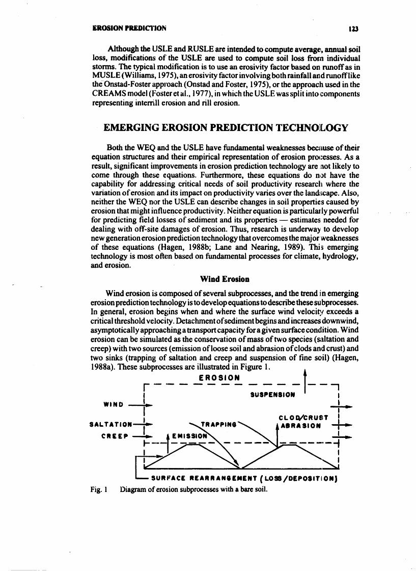
Wind erosion is composed of several subprocesses, and the trend in emerging erosion prediction technology is to develop equations to describe these su bprocesses. In general, erosion begins when and where the surface wind velocity exceeds a critical threshold velocity. Detachment of sediment begins and increases downwind, asymptotically approaching a transport capacity for a given surface condition. Wind erosion can be simulated as the conservation of mass of two species (saltation and creep) with two sources (emission of loose soil and abrasion of clods and crust) and two sinks (trapping of saltation and creep and suspension of fine soil) (Hagen, 1988a). These subprocesses are illustrated in Figure 1. A

E R O S I O N t

WIND 1, I

Fig. 1 Diagram of erosion subprocesses with a bare soil.

I24 SOIL EROSION AND SOIL PRODUCTIWTY

Forces acting during wind erosion include shearing stress of the wind at the soil surface, which moves loose particles; and impact stress of saltating particles.. which breaks down clods and crust to moveable sizes. Thus, soil erodibility depend-, on the size distribution ofsoil aggregates at the surface, the resistance of'the clods and crust to abrasion, and the threshold wind velocity at which particles begin to move on a given surfacc. Temporal soil properties that directly affect crodibil~ty i nclude density, dry stability, and size distribution of aggregates; density, dry stability. thickness, and cover fraction of crust; loose particles on the LNSL; soil wetness; and surface roughness.

The erosivity of the wind is reduced by vegetative cover. Standing vegetation increases both air turbulence and the shearing stress above the canopy compared to smooth soil (Lyles and Allison, 1979). Nevertheless, below the canopy, wind shear stress on the soil is reduced from what it would be with no cover. The sarch~~tecture of the canopy significantly affects these forces and their depletion through the canopy. The wind shearing stress at the soil surface belo% the canopy drives the erosion process. The decrease in shearing stress through the canopy has been postulated to be a fbnction of canopy cover (Gregory and Borrelli, 1986) or a function of leaf and stem projected area (Hagen and Lyles. 1988).

Flat residue also reduces the erosivity of wind (Flyrear, 1985). It protects part of the soil surface and increases the total aerodynamic roughness of the surface. A significant part of the air's total shear stress is expended on the flat residue rather than the soil. The effect of flat residue is related to the amount of the surface covered by the residue and the stability of the residue as affected by being partially buried or loose on the surface. Surface roughness, whether randoin or oriented in ridges, also reduces the erosivity of the wind. Shear stress can be so low in the depmssional areas that local deposition occurs. However, roughness loses its effectiveness over time, as these areas fill with sediment.

Process-based erosion prediction technology typically cornputes erosion on a storm by storm basis, and the more detailed models compute erosion by time steps within a stom. Because storage: of large serial weather records is not feasible, weather simulation generators and statistical data bases are being developed (Nicks et al., 1987; Skidmore and Tatarko, 1989) to provide the stochastic inputs. The generators will producc daily temperature maximums and minimums, solar radiation, daily precipitation, daily wind speed maximum and direction, imd subhourly wind speed distribution for the day. By using repeated random weather cycles for a given field rotation, a probability distribution of erosion loss can be computed for that given field. Other updated inputs also are required. Temporal c:hanges in variables such as soil moisture, surface roughness, and vegetative cover are updated by using submodels to simulate these processes or events, such as tillage.

Water Erosion

Emerging erosion prediction technology for erosion by water is based on mathematical relationships describing the hndamental erosim processes of de- tachment, transport, and deposition by the separate eroa ; ~ , e agents of raindrop impact and wface runoff. Also, the processes are group7 dccording to a source area concept to providc a way of spatially integrating poll.. proccsscs to represent large areas such as fields and farms. This approach rmimizes distortion of parameter values determined from small, idealized laboratc~~ a11d field experiments. Important source areas are interrill areas, rills, and c l herneral gullies, while

EROSION PREDICTION 1W

impoundments are often sinks. All represent hydrologic elements that can be linked together according to flow patterns on the landscape. These source areas and processes are illustrated in Figures 2 and 3.

_ _ - - - - - - - _ - _ W ~ t h ~ n

Flow D~recl~ons

Overland Flow

'teld Boundary

-I- Fig. 2 Source areas for water erosion.

Raindrop Impact I r- Detachment and Splash

-1'ransport bv Thin Flow

2,;. and Transport b), Flow

Rill Area

Fig. 3 Erosion prwesscs on rill and interrill areas.

The landscape containing the farm fields being analyzed is visualized as a set of overland flow areas and channel networks. Overland flow areas arc: areas where flow is uniformly distributed across the landscape, even though flow depth may be locally very nonunifonn. Most soil surfaces are nonuniform, causing flow to concentrate in many sm.al1 channels across the slope. If flow is sufficiently erosive in these flow concentrations, rills will develop, causing the flow to become even more concentrated in these channels. Typically, many rills develop across the slope, such that removal of a single rill will have little effect on the hydrologic and erosional response of the landscape. These flow concentrations are ciilled rill areas regardless of whether or not erosion occurs in them.

On the intemll areas, runoff occurs as a very thin, broad sheet. Interrill areas are defined such that all detachment occurring on them is by raindrop impact. Detached sediment is transported to the rills by splash from raindrop impact, a minor transport mechanism in most cases, and by the combined action of the thin surface flow on the interrill areas and the raindrop impact. Raindrop impact greatly enhances the transport capacity of the thin flow. Most of the downslope transport of sediment is in the rill areas.

126 !SOIL EROSION AND SOIL PRODUCTIVITY

The rill and intemll areas make up the overland flow area of a landscape. The topography of most fields is such that overland flow collects in a few major flow concentrations before leaving a field. Thus, runoff and sediment leave most fields at relatively few locations. Erosion can occur in these flow concentrations at amounts cqual to or grcatcr than the amount of sediment produced by rill and intcrrill crosiou. I:rosio~i III tlssc llow collca~tri~t i o t ~ s is ci~llctl ~ p l ~ ~ ~ l ~ c r i ~ l gully erosion. This erosion is fhdamentally the same as rill erosion and is described by the same relationships (Foster, 1986).

Both natural and constructed impoundments occur in fields. These areas of slowly moving water can d.eposit large amounts of sediment.

In general, the preference for describing detachment processes by either raindrop impact or surface flow is to write equations as a function of- the force applied to the soil at a point in time and space, relative to the resistance of the soil to disintegration when the stresses are applied to the soil. Erosion for a storm is calculated by integrating these equations over time for a single raindrop impact, over all the raindrops occurring in a storm, and over space for each hydrologic element.

Unfortunately, neither science nor computational power is sufficient to allow practical application of this very basic approach. Thus, emerging erosion prediction technology based on f'undamental processes involves empirical equations, having some similarity to the USLE, for each fundamental erosion process. Far example, detachment by raindrop impact is typically represented by the product of an erosivity term, like impact energy or rainfall intensity, which integrates over time, space, and raindrops, and iin erodibility factor that must be empirically measured. Similarly, detachment by flow is represented as the product of the difference of the shear stress of the flow acting on the soil minus a critical shear stress ofthe soil times an empirically measured erodibility factor. The influence of cover and management on erosion is considered by their effect on erosivity terms, such as shear stress and impact energy, and on erodibility terms. The basic concepts for describing these effects are much like those used to model wind erosion.

Slope steepness influences erosion by affecting the erosivity of raindrop impact and surface flow. The influence of slope length is described in the spatial integration of the continuity equation for mass transport. Deposition occurs at both micro and macro scales. An example of the micro scale is deposition in depressions left by tillage implements. An example at the macro scale is deposition at the base of a concave slope. In either case, deposition occurs when the rate of sediment arriving from upslope or from lateral areas exceeds the rate at which runoff can transport detached sediment. Depotsition is a very selective process and is typically described with equations that include a fall velocity term to account for both size and density of the sediment (Foster et al., 1983). Sediment eroded on agric:ulhulil fields is highly nonuniform, having particle sizes ranging from clay size to small gravel size and specific gravities ranging from about 1.5 to 2.7 (Foster et a1 ., 1985).

Equations for the capacity of runoff for transporting sediment are an important component of this technology. These equations, needed for both rill and intenill areas, are strong functions of flow hydraulics. On intemll areas, impacting raindrops significantly modify flow hydraulics, increasing the transpott capacity of thin flow. In situations where deposition occurs, the accuracy of the predictions depends much more on the deposition and transport relationships than on the detachment rela- tionships.

EROSION PREOICITON 127

As for wind erosion, values are needed for canopy, ground cover, roughness, incorporated crop residue, and odm similar variables that are influenced by cropping, management, wnd climate. These values are computed with submodels using equations for crop growth, residue decomposition, tillage, and soil water movement.

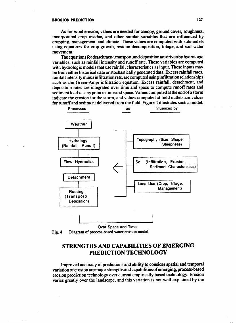
The equations for detachment, transport, and deposition are driven by hydrologic variables, suclh as rainfall intensity and runoff rate. These variables are computed with hydrologic models that use rainfall characteristics as input. These inputs may be from either historical data or stochastically generated data. Excess rainfall rates, rainfall intensity minus infiltration rate, are computed using infiltration relationships such as the Green-Ampt infiltration equation. Excess rainfall, detachment, and deposition rates are integrated over time and space to compute runoff rates and sediment loads at any point in time and space. Value2 computed at the end of a storm indicate the erosion for the storm, and values computed at field outlets are values for runoff and sediment delivered from the field. Figure 4 illustrates such a model.

Processes --

I Hydrology (Rainfall, Runoff) I Flow Hydraulics I - I I I Detachment I

Routing (Transport/

Deposition)

as Influenced by -

1

Topography (Size, Shape, Steepness) 1

Soil (Infiltration, Erosion, Sediment Characteristics)

1 1 Land Use (Crop. Tillage. Management) I

-

Over Space and Time Fig. 4 Diagram of process-based water erosion model.

STRENGTHS AND CAPABILITIES OF EMERGING PREDICTION TECHNOLOGY

Improved accuracy of predictions and ability to consider spatial and temporal variation of erosion are major strengths and capabilities of emerging, process-based erosion predict ion technology over current empirically based technology. Erosion varies greatly over the landscape, and this variation is not well explained by the

128 SOIL EHOSION ANI) W l L PWOUU4"1'1VI'I'Y

WEQ and USLE. The WEQ does not consider incoming sediment load, and the USLE does not estimate deposition and, thus, cannot deal with those portions of a landscape whcrc signiticant deposition occurs. On nonunitbml eroding portions of. landscapes, emerging technology better accounts for the eflects of varying topog- raphy than either the WEQ or the USLE, even though both can be modified to consider variation in erosion along r lu~ldscapc prdilc ( Foster olrd W iscllllsicr, 1 974).

Most landscapes are three dimensional causing divergence or convergence of surface runoff, which the two dimensional USLE does not take into account. Digital topographic modeling provides a model structure to apply to the hydrologic and erosion equations, so that three dimensional landscapes can be fblly analyzed (Moore et al., 1988). In addition to considering three dimznsional surface flow, these models can deal with three dimensional subsurfiwe flow and the resulting spatial variation in soil moisture that influences crop yield and erodibility of soil, especially in ephemeral gully areas. High rates of ephemetrl gully erosion cause incisement over time, significantly changing the landscape. This incisernent steepens areas adjacent to the gullies and accelerates nearby intemll and rill erosion. Also, annual tillage moves soil into the gullies, which contribures tt, further changes in the productive potential of soil in these areas. Process-based models have the capability of being able to compute these changes in the landscapz.

Another capability provided by process-based erosion prediction technology is the computation of frequency distributions of soil loss. 'Typically, soil loss is lognormally distributed in time (Wischmeier and Smith, 1978). The impact of a given soil loss occurring in one or two years may be greater or less than the effect if this same soil loss were to occur uniformly over time. A majar difficulty in conducting experimental research on the effi:ct of erosion on productivity is the variability of weather from year to year and the resulting variability in crop yield and erosion (Lyles, 1975). This variability can easily mask the effect of erosion. The capability to estimate erosion and its annual varinbili~ when combined with the capability to compute crop yield as a function of weather and soil variables affected by erosion provides a powerful tool to study the long-tenn effect of erosion on productivity, which cannot be easily studied in the field (Williams et al., 1984).

Process-based erosion prediction technology also can compute changes in soil properties as erosion progresses. Obviously changes in soil properties occur when there is a reduction in soil depth and the mixing of surface soil with deeper soil. These changes can be computed with existing technology (Williams et al., 1984). However, erosion is a selective process that tends to remove !;oil fines, while leaving coarse particles. Emerging erosion prediction technology can compute this en- richment of soil by coarse particles, which affects infiltration, erodibility, and soil moisture-holding capacity (Hagen and Lyles, 1985; Zobwk and Fryrear, 1986, Foster et al., 1983). Thus, productivity estimaies can be related to the soil remaining rather than to the soil lost.

Not only can the change in soil properties at a locarion in a field be computed, the characteristics of the sediment as it moves over the d surface as saltation, creep, and suspension in wind or as transported by r l . .,ff can be computed. Examining output at field outlets makes available estirn.t:t kj of sediment amounts and characteristics that are needed in assessing off-site iiin wcts of erosion.

EROSION PREDICTION

EXAMPLES OF PROCESS-BASED EROSION PREDICTION TECHNOLOGY

Several process-based erosion models have been developed. The well known models for water erosion include the CREAMS, ANSWERS, AGNPS, and SEDIMOT I 1 models. The wind erosion models include models by Gillette (1986) and Gregory and coworkers ( 1 988). Two major efforts led by thc USDA-Agricultural Research Service (ARS) are underway to develop process-based erosion prediction technologies to replace ihe WE? and USLE.

Water Erosion

The CREAMS model (Knisel, 1980) includes a process-based erosion compo- nent and was developed to analyze the effect of management practices on nonpoint source pollution from field-sized areas. The model considers nonuniform slopes, ephemeral gully erosion, and selective deposition. Intenill erosion and rill erosion are computed with a modificati~n of the USLE, whereas ephemeral gully erosion is computed with a prccess-based equation for detachment by flow. Sediment transport and deposi~ion are computed with modifications of the Yalin and Einstein equations for nonuniform sediment. The model uses a system of hydrologic elements that allows its application to a range of situations, including the usual overland flow-ephemeral gully erosion field representation, a ridge-furrow surface configuration, and a field with a system of gradient terraces. This model has been used to analyze the effect of nonuniform erosion on soil productivity along complex slopes (Perrens et al., 1085).

The ANSWERS and AGNPS models are watershed models that deal with nonpoint source pol Jution problems on areas ranging From fields to large areas of hundreds of hectares (Beasley et al., 1 980; Young et al., 1987). These models use square grid elements to deal with spatial variability of erosion. They can be applied to study the effects of spatial variability of erosion on productivity over large areas although their definition of local areas within a field are limited in those cases.

The SEDIMOT I1 model was developed primarily for application to surface- mined areas (Wilson et al., 1 986). Its main strengths are the process-based equations for the effect of structurc:~ like impoundments and porous dams on deposition. It also has a flexible system that allows linking of overland flow areas and chamel reaches to represent very complex areas. Like CREAMS, it uses a typical slope profile to represent overland flow subareas rather than a grid network.

A major drawback to these models and similar ones is that they are much more difficult to use than the USLE. Another major drawback is that they either use the USLE, some form of it, or USLE parameter values for the governing erosion equations, or they use parameter values based on very limited data. Also, few of the existing process-based models have been extensively validated.

A major project i:; underway to produce erosion prediction technology to overcomc these shortcomings. This project, the USDA-Water Erosion Prediction Project (W EPP) led by IWS (Lane and Nearing, 1989) also involves the USDA-Soil Conservation Service (SCS) and Forest Service, the USDI-Bureau of Land Man- agement, and seven1 other cooperators. This project is giving special attention to developing process-ba.sed erosion prediction technology that is easy to use. In

130 SOIL EROSION AND SOIL PRODUCTIVITY

addition to research developing analyucal compnents, the project has a major experimental program to collect data needed ti, develop the parameter values required by the specific process-based equations rather than adapting values fiom the USLE.

In August 1989, the project delivered the first version of the model to the cooperating action agencies. Research continues to refine the model and to produce data needed to determine additional parameter values. Also, motkl verification and validation is underway along with development of computer software to mike the model easy to use. Widespread application of the model is expected by the mid 1990's.

Wind Erosion

Recent numerical simulations of saltation on sand sUTfwes have improved the understanding of several wind erosion processes, ranging From aerod-mamic entrainment of the initial grains to the final downwind steady-sute flux (Anderson and Haff, 1988). In addition, a wide range of monodisperse particle surfaces have been studied in wind tunnels, and their threshold velocities ars well-documented (Greeley and Iverson, 1 985).

Gillette (1 986) has proposed a mixed empirical and process-based prediction equation. It sums erosion using wind speed distribution above threshold wind speeds but requires users to input all erodibility parameters and their changes over time. Gillette and Passi (1990) recently used a modification of that eqwtion to estimate atmospheric dust input in the US. Gregory and coworkers (1 988) devel- oped a steady-state expression for the increasc in soil discharge along the wind direction. The form of their model is:

x=C(SU~ - u$J.(l-e--) where: X = rate ofhorizontal soil movement at downwind length L, C = an empirical coefficient, S = fraction of shesuing stress above the soil cover hansferred to the soil surface, U, = Friction velocity, U,, = threshold friction velocity, d = a constant, A = abrasion adjustment coefficient that is a function of 1 and L, 1 = soil ewdibility coefficient that is a function of soil shear strength and soil shear angle, and L := length of unprotected field in direction of the wind. Using an iterative approach, they applied their equation to a series of successive field segments with differini; covers and erodibilities. The term C(SU:-u:,)u, represents the maximum rate of soil movement as L approaches infinity. For a bare soil with S equal 1, the term is identical to one of the several empirical transport equations reported by Gredey and Iverson (1985). The last bracketed term in the Gregory et a.1. model forces the transport rate to approach a maximum asymptotically. The soil erodibilit) term is based on the finding by Nearing and Bradford (1985) that detachment by thc impact of a single water drop is related to soil shear strength and shear angle.

The user of the Gregory et al. model must continually update parameter values for the surface conditions in order to compute soil loss over any time period during which the surface or the wind direction changes. If the distance L varies along the downwind field boundary, soil loss must be computed for varying L and integrated

- along the downwind boundary to compute field soil loss. In 1986, a wind erosion modeling team c:omposed of USDA scientists fiom

ARS and SCS began work on a comprehensive model to replace the current WEQ.

EROSION PREDICTION 131

The model de:velopment process has two major stages. The objective of the first stage is to develop e wind erosion research model (WERM), which will be a daily simulation model that will be validated and used as a reference standard for wind erosion predictions (Hagen, 1988b). The WERM model is scheduled to be opera- tional in 199 1.

In the second stage of development, the submodels in WERM will be reorga- nized to impnwe computation speed, the data bases will be expanded in size, and a user-friendly inpurfoutput section will be added to produce the final wind erosion prediction system (WEPS) that will be used by action agencies.

The structure of \WRM is modular and consists of a main, supervisory program; a usw-interfaoe input section; seven submodels along with their associ- ated data bases; and an output control section (Figure 5).

W E R M

C M A I N . - . - 7 7 - - - - - - - -

F t F I L E S

I

O U T P U T

CONTROL

O U T P U T

F I L E S

C R O P 4 G R O W T H I

tC( E R O S I O N I

Fig. 5 Diagram of Wind Erosion Research Model (WERM) with associated files and data bases.

132 SOIL EROSION AND !i011, YWOU1JC"I'IVI'I'Y

Major submodels include components for crop growth, decomposition of crop residue, soil condition, hydrology, and tillage, which predict the temporal changes in soil and vegetative cover variables in response to inputs generated by the weather submodel. Finally, if wind speeds exceed the critical threshold velocity, the erosion submodel computcs soil loss or deposition over the simulation region.

SUMMARY

Erosion prediction is a powerful tool that has been used by soil conservationists since the 1940's. Most conservation farm planning is done using the empirical Wind Erosion Equation ( W EQ) and the empirical Universal Soil Loss Equation (USLE) for sheet and rill erosion. These equations can identify situations where erosion is considered to be excessive and guide the selection of practice3 that will adequately control erosion. These equations also have been applied in national inventories of erosion to assess its impact on nonfederal land and are being used to implement public soil conservation policy embodied in the 19115 Food Security Act.

These empirical erosion prediction technologies have important limitations when used to analyze the impact of soil erosion on productivity. New process-based erosion prediction technologies are emerging to replace these empirical technologies. In addition to providing estimates with improved accuracy, these new technologies have much expanded capabilities for computing the temporal and spatial variability of erosion.

Two important cooperative efforts, the Wind Erosion Prediction Systems ( WEPS) project and the Water Erosion Prediction Project ( W EPP), are developing process-based erosion prediction technologies for wind and water erosion, respec- tively, for use by action agencies. These technologies, expected to replace the WEQ and USLE, should be widely available by the mid 1990's. They will be available for research applications much sooner. Both of these projects are led by the USDA- Agricultural Research Service in cooperation with other agenc ies and organizations.

While these technologies are being developed, the WEQ and the USLE will continue to be used. The USLE is being revised and updated extensively, resulting in RUSLE, Revised USLE, which should be available by late 1990. This effort is also being led by the USDA-Agricultural Research Service.

REFERENCES

Anderson, R. S. and P. K. Ha& 1988. Simulation of eolian saltation. Science 24 1 :820- 823.

Bagnold, R. A. 1941. The physics of blown sands imd desert dunes. Chapman and Hall. London, England. 265 pp.

Beasley, D. B., L. F. Huggins, and E. J. Monke. 1980. ANSWERS: A model for watershed planning. Transactions of the American Society of Agricultural Engineers 10:485-492.

Bondy, E., L. Lyles, and W. A. Hayes. 1980. Computing soil erosicm by periods using wind energy distribution. Journal of Soil and Water Cunservatinl 1 : 173- 1 76.

Colacicco, D., T. Osbom, and K. Alt. 1989. Econmic damag~ ii m soil erosion. Joumal of Soil and Water Conservation 4435-39.

Cole, G. W.. L. Lyles, and L. 1. Hagen. 1983. A s m ulation motld uf daily wind erosion soil loss. Transactions of the American Society of ~gricultural i nj:ineers 26: 1758- 1765.

Cook, H. L. 1936. The nature and controlling variables of the water erosion process. Soil Science Society of Amehca Proceedings 1 :487-494.

Davis, R. and G. D. Cr~ndra. 1988. The on-site casts of wind erosion on fences in New Mexico. Proceedings 19:38 Wind Erosion Conference. Texas Tech University. Lubbock, TX. pp. 238-264.

Follett, R. F. and B. A. Stewart (editors). 1 985. Soil Erosion and Crop Productivity. American Society of Agronomy. hiadison, WI. 533 pp.

Foster, G. R 1986. Understanding ephemeral gully erosion. In: Soil Conservation: Assessing the National Resources Inventory. Volume 2. Wolman, M. G. et al. (editors). National Academy Press. Washington, M3. pp. 90- 1 25.

Foster, G. R., L. J. Larre, 3. D. Nowlin, I. M. Laflun, and R. A. Young. 1983. Estimating erosion and sediment yield on field-sized areas. Transactions of the American Society of Agricultural Engineers :!4: 1 253- 1 262.

Foster, G. R., F. Lombardi, and W C. Moldenhailer. 1982. Evaluation of rainfall-runoff erosivity factors for individual storms. Transactionsofthe American Society ofAgicultura1 Engineers 25: 124- 1 29.

Foster, G. R . , L. D. Mey er, imd C. A. Onstad. 1977. An erosion equation derived fiom basic erosion principles. Tratlslrctions of the American Society of Agricultural Engineers 20:678-(is:!.

Foster, G. R., R. A. Yomg, and W. H. Neibling. 1985. Sediment composition for nonpoint source pollution ana1yse.i. Transactions of the American Society of Agricultural Engineers 28: 133- 13!).

Foster, G. R. and W. H. Wischmeier. 1974. Evaluating imgular slopes for soil loss prediction. Transaclionc. of the American Society of Agricultural Engineers. 17:305-309.

Fryrear, D. W. 1988. Scil Cover and wind erosion. Transactions of the American Society of Agricultural Engincers 28:78 1 -784.

Gillette, D. A. 1986. W lnd crosion. In: Soil Consenration: Assessing the National Resources Inventoky. Volume 2. Wolman, M. G. et al. (editors). National Academy Press. Wash- ington, IX:. pp. 129- 1 58.

Gillette, D. A. and R. Passi. 1990. Modeling dust emission caused by wind erosion. (submitted1 for publication).

Greeley, R. and J. D. Iverson. 1985. Wind as a geological process. Cambridge University Press. Carnbridge,E:nglond. 333 pp.

Gregory, J. M. and J. Borr~:lli. 1986. Physical concepts for modeling soil erosion by wind. Paper No. S WR86- 002. American Society of Agricultural Engineers. St. Joseph, MI.

Gregory, J. hl., J. Borrelli, and C. B. Fedler. 1988. Team: Texas erosion analysis model. Proceedings 1988 Wind Erosio~k Confcrencc, Texas Tech University. Lubbock. TX. pp. 88- 103.

Hagen, L. J. 1988a. Wrnd erosion mechanics: abrasion of an aggregated soil. Paper No. 88- 256 1. American Society of Agricultural Engineers. St. Joseph, MI.

Hagen, L. J. 1988b. Winti crosiorl prediction system: an overview. Paper No. 88-2554. American Society of Agricultual Engineers. St. Joseph, MI.

Hagen, L. J. ilnd L. Lyles. 1985. Amount and nutrient content of particles produced by soil aggregate abrasion. In: Erosion and Soil Productivity. Publ. No. 8-85. American Society of Agricultural Engineers. St. Joseph, MI. pp. 1 17-129.

Hagen, L. J. itnd L. Ly les. 1 988. Estimating the small grain equivalents of shrub-dominated rangelandis for wind erosion control. Transactions of the American Society of Agricul- tural Engineers 3 1 : 769-775.

Hagen, L. J. and N. P. Woodruff. 1973. Air pollution fiom dust storms in the Great Plains. Atmosph~aric Enviro~~ent 7:323-332.

134 SOIL EROSION AND SOIL PRODUCTIVITY

Huzar, P. C. and S. L. Piper. 1986. Estimating the crffsite costs of wind erosion in New Mexico. Journal of Soil and Water Conservation 4 1 :4 14-4 16.

Knisel, W. G . 1980. CREAMS: A Field Scale Model for Chemicals, Runoff; and Erosion from Agricultural Management Systems. Conservation Research Report No. 26. USDA- Agricultural Research Service. Washington, DC. 643 pp.

Lane, L. J. and M. A. Nearing. 1989. Profile Model Documentation. IJSDA- Water Erosion Prediction Project (WEPP). NSERL Report No. 2. National Soil Erosion Research Laboratory. USDA-Agricultural Research Service. W. Lafayctte, IN.

Lyles, L. 1975. Possible effects of wind erosion on soil productivity. Journal of Soil and Water Conservation 30:279- 283.

Lyles, L. 1983. Erosive wind energy distributions and climate factors for the west. Journal of Soil and Water Conservation 38: 106- 109.

Lyles, L. 1985. Predicting and controlling wind emsron. Agricultural History 59:205-2 14. Lyles, L. and B. E. Allison. 1979. Wind profile parameters and turl~ulencz intensity over

several roughness element geometries. Transactions ofthe American Society of Agricultural Engineers 22:334-338,343.

Lyles, L. and J. Tatarko. 1986. Wind erosion effects on soil tcxtue and organic matter. Journal of Soil and Water Conservation 4 1 : 19 1 - 193.

Moore, I. D., J. C. Panuska, R. B. Grayson, and K. P. Srivastava. i 988. Application of digital topographic modeling in hydrology. In: Modeling Agricultural, Forest, and Rangeland Hydrology. American Society of Agricultural Engineers. St. Joseph, MI. pp. 447-46 1.

Nearing, M. A., and J. M. Bmdford. 1985. Single water drop splash detachment and mechanical properties of soils. Soil Science Society of Amcrica Journal 49: 54.7-552.

Nicks, A. D., J. R. Williams, C. W. Richardson, and L. J. Lane. 1987. Generating climatic data for a water erosion prediction model. Paper No. 87-2541. American Society of Agricultural Engineers. St. Joseph, MI.

Onstad, C. A. and G. R. Foster. 1 975. Erosion modelmg or a watershed. Transactions of the American Society of Agricultural Engineers. 1 8: 288-292.

Perrens, S. J., G. R. Foster, and 13.8. Beasley. 1985. Erosion's effect on productivity along nonuniform slopes. In: Erosion and Soil Productivity. Publ. No. L-85. American Society of Agricultural Engineers. St. Joseph, MI. pp. 20 1-2 14.

Piest, R. F., L. A. Kramer, and H. G. Heineman. 1975. Sediment movement from loessial watersheds. In: Present and Prospective Technology for Predicting Sediment Yields and Sources. ARS-40. USDA-Agricultural Research Service. Washington, D.C. pp. 130- 14 1.

Renard, K. G., G. R. Foster, G. A. Weesies and J. P. Porter. 1989. RUSLE-The Revised Universal Soil Loss Equation. Presented at the 1989 Annual Meeting. Soil and Water Conservation Society. Ankeny, IA.

Skidmore, E. L. 1986. Wind erosion climatic erosibity. Climatic Change 9: 195-208. Skidmore, E. L. 1987. Wind erosion direction factors as influenced by field shape and wind

preponderance. Soil Science Society of America Journal 5 1 : 198-202. Skidmore, E. L. and J. Tatarko. 1989. Wind in the Great Plains: speed and direction

distributions by month. Proceedings of Symposium Toward a Sustainable Agricultwe for the Great Plains. Colorado State University. Fort Collins, Color ado. (abstract).

Smith, D. D. and D. M. Whitt. 1947. Estimating soil losses fiorn field areas of claypan soil. Soil Science Society of America Proceedings. l2:485-490.

Williams, J. R. 1975. Sediment yield prediction with Universal Equation using runoff energy factor. In: Present and Prospective Technology for Predhctinj Sediment Yields and Sources. ARS-40. USDA-Agricultural Research Service. Washington, DC. pp. 244-252.

EROSION YREIBICTICbN 135

Williams, J., C. A. Jorres, cud P. T. Dyke. 1984. A modeling approach to determining the relationship between erosion and soil productivity. Transactions of the American Society of Agricultural Engineers 27: 129- 144.

Wilson, B. N., El. J. Barfield, and R. C. Warner. 1986. Simple models to evaluate non-point pollution sources and controls. In: Agricultural Nonpoint Source Pollution: Model Selection antl Application. A. Giwgini and F. Zingales (ed). Elsevier. New York, NY. pp. 23 1 -263.

Wischmeier, W. H.. C. B. Johnson, and 8. V. Cross. 197 1. A soil erodibility nomograph for farmland antl const~uctions sites. Jownal of Soil and Water Conservation 26: 189-193.

Wischmeier, W. H. and D. 1). Smith. 1978. Predicting rainfall erosion-a guide to conser- vation planning. Agiculture Handbook 537. U.S. Department of Agriculture. Washington, DC. 58 pp.

Wolman, M. G. and others (editors) 1986. Soil Conservation: Assessing the National Resources Inventory. Volume 2. National Academy Press. Washington, DC. 3 14 pp.

Woodruff, W. P. and F H. Siddoway. 1965. A wind erosion equation. Soil Science Society of America Proceeding:; 29:602-608.

Young, R. A., C. A. Onstad, D. D. Bosch, and W. P. Anderson. 1987. AGNPS, Agricultural Non-Point-Source Pollution Model; A Watershed Analysis Tool. Conservation Research Report No. 3 5. USLIA-Agricultural Research Service. Washington, DC. 77 pp.

Zingg, A. W. 1940. Degree and length of slope as it affects soil loss in runoff. Agricultural Engineering 2 1 59-64.

Zobeck, T. M. and D. W. Fryrear. 1986. Chemical and physical characteristics ofwind blown sediment 11. Chemical characteristics and total sail nutrient discharge. Transactions of the American Society of Agricultural Engineers 29: 1037- 104 1.