soil degradation and sustainable land management in the rainfed
TRANSCRIPT
THE ECONOMICS OF LAND DEGRADATION
Soil Degradation and Sustainable Land Management in the Rainfed Agricultural Areas of Ethiopia: An Assessment of the Economic Implications
Ethiopia Case Study
www.eld-initiative.org
2
Suggested citation:
Hurni K, Zeleke G, Kassie M, Tegegne B, Kassawmar T, Teferi E, Moges A, Tadesse D, Ahmed M, Degu Y, Kebebew Z, Hodel E, Amdihun A, Mekuriaw A, Debele B, Deichert G, Hurni H. 2015. Economics of Land Degradation (ELD) Ethiopia Case Study. Soil Degradation and Sustainable Land Management in the Rainfed Agricultural Areas of Ethiopia: An Assessment of the Economic Implications. Report for the Economics of Land Degradation Initiative. 94 pp.
Available from: www.eld-initiative.org
Report Main Contributors:
Kaspar Hurni; Gete Zeleke; Menale Kassie; Berhan Tegegne; Tibebu Kassawmar; Ermias Teferi;
Aderajew Moges; Deme Tadesse; Mohamed Ahmed; Yohannes Degu; Zeleke Kebebew; Elias Hodel;
Ahmed Amdihun; Asnake Mekuriaw; Berhanu Debele; Georg Deichert, and Hans Hurni
Editing: Naomi Stewart (UNU-INWEH), and Marlène Thiebault (CDE; for the Executive Summary and Chapter 3)
Reviewers: Dr Berhanu Gebremedhin, Dr Emmanuelle Quillérou
This report was prepared by and published with the support of:
Water and Land Resource Centre (WLRC), Addis Abeba,
Centre for Development and Environment (CDE) of the University of Bern,
and Deutsche Gesellschaft für Internationale Zusammenarbeit (GIZ) GmbH
on behalf of the German Federal Ministry for Economic Cooperation and Development (BMZ).
Photography: Hans Hurni (cover and p 12), Tibebu Kassawmar (p 22, 24, 26, 29)
Visual Concept: MediaCompany, Bonn Office
Layout: kippconcept GmbH, Bonn
Links: http://wlrc-eth.org
http:// www.cde.unibe.ch
http://www.giz.de
http://eld-initiative.org
For further information and feedback please contact:
ELD Secretariat
Mark Schauer
c/o Deutsche Gesellschaft für Internationale Zusammenarbeit (GIZ) GmbH
Godesberger Allee 119
53175 Bonn, Germany

Soil Degradation and Sustainable Land Management in the Rainfed Agricultural Areas of Ethiopia: An Assessment of the Economic Implications
2015
Economics of Land Degradation Initiative:Ethiopia Case Study
www.eld-initiative.org

4
Acknowledgements:
The authors of this report are very grateful to have obtained the opportunity of carrying out the ELD Ethiopia Case
Study between January and July 2014. In particular, our thanks go to Dr. Anneke Trux, head of the Convention Project
to Combat Desertification of GIZ in Bonn until August 2013. Dr. Trux had discussed the idea of such a study in July 2013
with Dr. Johannes Schoeneberger, head of the SLM Project of GIZ in Ethiopia, who approved it and welcomed the
idea of getting the University of Bern involved. From the beginning, Mr. Mark Schauer (coordinator of the ELD
Secretariat) and Ms. Bettina Streiter-Moll, both of GIZ, were part of the organizing team, making it possible to
develop a project proposal and respective agreements, and get them approved and signed within a few months’ time.
After the start of the project, a very close follow-up between the project director and Mr. Hannes Etter of GIZ was
assured through swift email exchanges whenever there were open questions. Furthermore, we would like to thank
Dr. Emmanuelle Quillérou and Dr. Berhanu Gebremedhin for the review of the report, and Ms. Naomi Stewart
(UNU-INWEH) and Ms. Marlène Thiebault for editorial assistance and language editing. Without such supportive
contributions, it would have been much harder to achieve the current results.
A N E L D A S S E S S M E N T
5
Executive summary
The Economics of Land Degradation (ELD) Initia-tive is an initiative on the economic benefits of land and land-based ecosystems. The initiative high-lights the value of sustainable land management and provides a global approach for analysis of the economics of land degradation. This report sum-marizes the findings of a case study of the ELD Ini-tiative in Ethiopia. The case study was commis-sioned by GIZ and carried out by the Centre for Development and Environment (CDE) and the Water and Land Resource Centre (WLRC) from Jan-uary to July 2014.
Ethiopia is known for its historic agriculture, but also for the associated, widespread, and on-going land degradation. The older agricultural areas of the northeast have long been particularly affected, but the highest soil erosion rates are currently being observed in the western parts of the high-lands. The processes of soil erosion and measures to reduce it have been researched extensively in Ethi-opia since the 1970s; research activities include long-term monitoring of catchments and experi-ments of various spatial extents. On this basis of understanding and data availability, Ethiopia offered a unique setting for an ELD case study.
This case study provides a spatially explicit assess-ment of the extent of land degradation (soil erosion by water) and the costs and benefits of sustainable land management measures. The focus is on areas under rainfed cultivation. The unit of analysis is a pixel of 30 m by 30 m, in line with the resolution of the Landsat imagery used for assessing land cover. The case study area covers 600,000 km2 or about 54 per cent of Ethiopia’s territory, more than 660 mil-lion pixels. Of the included pixels, about 239 mil-lion were identified as cropland, amounting to about 215,000 km2 – a surprisingly large area com-pared to the current statistics that indicate a grain crops area of approximately 123,000 km2 (CSA 2013a). The dry lowland areas without rainfed cul-tivation were not considered in the analysis.
The project team worked in small groups, each of which provided unique insights towards an eco-
nomic valuation of ecosystem services and their importance for the livelihoods of communities. The main focus was on the productive functions of land, as this matters most to small-scale farmers. To provide an economic analysis of these functions, authors looked at different scenarios of sustainable land management implementation over the next 30 years. Other ecosystem functions such as supply of water and sediments to lowland areas and resto-ration of soils through soil and water conservation as well as off-site impacts of soil erosion were not fully included in the economic analysis. The omis-sion of such ecosystem functions in this analysis, is likely to underestimate the benefits of sustainable land management interventions.
Land cover was mapped using an approach that combined visual delimitation of units of analysis with expert knowledge and automated image clas-sification. This approach made it possible to distin-guish cultivated land (i.e., cropland, which in Ethi-opia consists of land currently being ploughed or harvested, land with growing crops, land under mixed crop and trees system, and fallow land) from other land use or land cover classes. Unsurpris-ingly, the actual amount of cultivated land is con-siderably larger than that indicated by official sta-tistics in use since the mid-1980s, when the rural population was half its current size. The team also mapped large-scale land use systems, inclusive of any foreign direct investments. Results of the study show there has been a considerable expansion and intensification of farming in the past three dec-ades, leading to more soil erosion.
Conservation structure mapping was attempted by an automated procedure of reading linear struc-tures from Google Earth images. However, this approach failed because of the low accuracy of the resulting maps. The team then devised an approxi-mate expert-based modelling approach, built on the assumption of experts that conservation struc-tures existed in about 18 per cent of the country’s cropland in 2014, as well as other assumptions about their spatial distribution (e.g., slope and travel time to the cropland from the villages).
6
Soil erosion and deposition values were estimated using pixel based landscape information and the Unit Stream Power Erosion Deposition (USPED) model, which works with the Universal Soil Loss Equation (USLE) parameters. The USPED model was adapted to Ethiopian conditions based on evidence from the Soil Conservation Research Programme, and calibrated and validated using data from for-mer research stations as well as the Abbay (Blue Nile) Basin. Additionally, some of the USLE param-eters were reduced in order to achieve a satisfac-tory approximation of sediment loss for the Abbay Basin.
These adaptations made it possible to produce a pixel based soil erosion and sediment deposition model for the whole study area and even more importantly, to run different scenarios of invest-ments in the cropland and show their effects after 30 years. However, these scenarios did not consider climate change or changes in the extent of the cropland. Based on net erosion/deposition esti-mates produced by the USPED model, the present annual net erosion across the study area is –940 million tonnes, or –18 tonnes/ha. This estimate con-siders currently existing conservation structures, which are present in about 18 per cent of cropland on slopes > 8 per cent in the study area of the USPED model. However, the share of cropland situated on slopes steeper than 8 per cent totals 77 per cent, which means that such area needs soil and water conservation. As a result, conservation structures would need to be built on an additional 59 per cent of cropland (about 12.7 million ha), in order for all sloping cropland to be conserved. Looking exclu-sively at cropland, the model produced an annual net erosion of –380 million tonnes (–20.2 tonnes/ha). This value could be reduced to –222 million tonnes (–11.8 tonnes/ha) if conservation structures were constructed on all sloping cropland.
The situation is similar in the Grand Ethiopian Renaissance Dam Basin: additional structures in cropland on slopes > 8 per cent could reduce over-all net erosion in all land cover classes by 21 per cent, and net erosion in cropland by as much as 43 per cent. In absolute values, this would mean a reduction from –320 million tonnes/yr to –251 mil-lion tonnes/yr, a number that could be further reduced when applying conservation measures on all landscapes. However, it should be noted that while the USPED model was calibrated to deliver
the ~300 million tonnes of sediment yield esti-mated for the GERD, it is not exactly known when and how this value was measured or estimated (cf. Abdelsalam 2008).
After modelling soil erosion/deposition for two sce-narios (current distribution of conservation struc-tures, and conservation structures on all cropland steeper than 8 per cent), crop production was esti-mated for a time period of 30 years, based on rela-tionships between production and soil depth. The estimation algorithm was calibrated using infor-mation on productivity from reports of the Central Statistical Agency of Ethiopia. The two soil erosion/deposition scenarios assuming different distribu-tions of conservation structures were then aug-mented with two more scenarios, one assuming the current extent of fertilizer application and the other assuming fertilizer application on all crop-lands. On this basis, crop production was estimated over the coming 30 years for the four scenarios as:
1. current distribution of conservation structures and currently fertilized croplands;
2. current distribution of conservation structures and fertilizer application on all cropland;
3. conservation structures on all sloping cropland and currently fertilized croplands, and;
4. conservation structures on all sloping cropland and fertilizer application on all cropland.
This analysis showed that Scenario 1 (‘business as usual’) results in a reduction of crop production by more than 5 per cent over 30 years. The other three scenarios show a crop production similar to cur-rent values (Scenario 3) or an increase of about 3 per cent (Scenario 2) and about 10 per cent (Scenario 4). Even if these increases seem moderate, the model-ling exercise indicates that crop production can be maintained or slightly increased by applying sus-tainable land management practices, whereas crop production decreases if none are applied.
The profitability of each management option was then assessed by performing a cost-benefit analy-sis. The number of scenarios increased from four to eight by performing two versions of the cost-bene-fit analysis for each scenario: one assuming planta-tion of fodder grass on all conservation structures and the other assuming no plantation of fodder grass. Growing fodder grass on the structures increases the productivity of conserved farmland
A N E L D A S S E S S M E N T
7
due to the production on the otherwise unused area of the conservation structure. A variety of such management options exist (e.g., growing fruit trees or high-value legumes), but were not consid-ered in the study due to lack of data. The authors believe that including such management options in the analysis upon data availability is likely to increase the benefits of conservation structures. For each of the eight scenarios, respective costs and benefits were defined and the cost-benefit analysis was performed at pixel level for the 30 years, assum-ing a discount rate of 12.5 per cent. To compare the scenarios and determine the most profitable man-agement option or combinations of options for a given area, net present value was calculated for each scenario at pixel level and summarised by administrative unit.
Comparison of the different scenarios’ net present values at wereda level showed that soil and water conservation measures combined with fertilizer application and fodder grass generally have a posi-tive net present value suggesting investment in sustainable land management is profitable, all else being equal. However, there are regional differ-ences: in Tigray, for example, a large number of conservation structures have already been built; accordingly, the net present value can be increased only by additionally planting fodder grass on the conservation structures. In areas where soils are shallow, i.e., some parts of the Amhara Region, building conservation structures and planting fod-der grass on them is profitable, whereas fertilizer application has a limited effect due to shallow soils and thus cannot increase production enough to compensate for fertilizer costs. Across most of the Oromia, Benishangul-Gumuz, and Southern Nations, Nationalities, and Peoples’ (SNNP) regions, the full range of management options that include conservation structures, fertilizer application, and fodder grass, is the most profitable scenario.
In addition to comparing scenarios, the relation-ship between the current soil erosion rate and the net present value of the best management option for each area was also examined. This information is useful for planning development interventions to reduce soil erosion: for example, with the best management option, areas with a high erosion rate and a low net present value are likely to need more support than areas with a low erosion rate and a high net present value. Spatial differentiation is
thus key in prioritizing development interventions and implementation. The ELD Ethiopia Case Study database provides an excellent source of data for such differentiation.
8
Abbreviations and Amharic terms
Berha Desert belt (very hot and arid)
CBA Cost-benefit analysis
CDE Centre for Development and Environment, University of Bern
CSA Central Statistical Authority of Ethiopia
DAP Di-Ammonium Phosphate, fertilizer
Dega Highland belt (cool, humid)
DEM Digital Elevation Model
ELD Economics of Land Degradation
ETB Ethiopian Birr
EUR Euros
FAO/LUPRD Food and Agriculture Organization
GERD Grand Ethiopian Renaissance Dam
GIS Geographic Information System
HICU Homogenous Image Classification Unit
Inset False banana
Kebele Community below wereda
Kolla Lowland (semi-arid to sub-humid hot) belt
LULC Land Use and Land Cover
N Nitrogen (in soil)
NPV Net Present Value
P Phosphorus (in soil)
Region National state (below federal state), with governmental status
RUSLE Revised Universal Soil Loss Equation (model)
SCRP Soil Conservation Research Programme
SLM Sustainable Land Management
SNNP Southern Nations, Nationalities and Peoples’ (Region)
SWC Soil and Water Conservation
Tef Eragrostis tef (a major crop endemic to Ethiopia)
Urea Urea or carbamide, nitrogen-release fertilizer
USLE Universal Soil Loss Equation (model)
USPED Unit Stream Power Erosion Deposition (model)
Wereda District, administrative unit between zone and kebele
Weyna Dega Middle altitude warm and humid belt (optimum for agriculture)
WLRC Water and Land Resource Centre, Addis Abeba
Wurch Frost belt (cold)
Zone Administrative unit between region and wereda
A N E L D A S S E S S M E N T
9
Table of contents
Executive summary . . . . . . . . . . . . . . . . . . . . . . . . . . . . . . . . . . . . . . . . . . . . . . . . . . . . . . . . . . . . . . . . . . . . 5
Abbreviations and Amharic terms . . . . . . . . . . . . . . . . . . . . . . . . . . . . . . . . . . . . . . . . . . . . . . . . . . . . . 8
Table of contents . . . . . . . . . . . . . . . . . . . . . . . . . . . . . . . . . . . . . . . . . . . . . . . . . . . . . . . . . . . . . . . . . . . . . . . . 9
Chapter 1 Background . . . . . . . . . . . . . . . . . . . . . . . . . . . . . . . . . . . . . . . . . . . . . . . . . . . . . . . . . . . . . . . . . . . . . . . . . . . . 12
1.1 The ELD Initiative . . . . . . . . . . . . . . . . . . . . . . . . . . . . . . . . . . . . . . . . . . . . . . . . . . . . . . . . . . . . . . . . . . . 121.2 Land and soil degradation in the Ethiopian Highlands . . . . . . . . . . . . . . . . . . . . . . . . . . . . 121.3 Contribution to the goals of the ELD Initiative . . . . . . . . . . . . . . . . . . . . . . . . . . . . . . . . . . . . . 131.4 Location and scope . . . . . . . . . . . . . . . . . . . . . . . . . . . . . . . . . . . . . . . . . . . . . . . . . . . . . . . . . . . . . . . . . 131.5 Framework . . . . . . . . . . . . . . . . . . . . . . . . . . . . . . . . . . . . . . . . . . . . . . . . . . . . . . . . . . . . . . . . . . . . . . . . . 16
Chapter 2 Components of the ELD Ethiopia Case Study . . . . . . . . . . . . . . . . . . . . . . . . . . . . . . . . . . . . . . . . . . . 18
2.1 Component 1: Land cover mapping . . . . . . . . . . . . . . . . . . . . . . . . . . . . . . . . . . . . . . . . . . . . . . . . . 18
2.1.1 Background and scope . . . . . . . . . . . . . . . . . . . . . . . . . . . . . . . . . . . . . . . . . . . . . . . . . . . . . . . 182.1.2 Data and methodology . . . . . . . . . . . . . . . . . . . . . . . . . . . . . . . . . . . . . . . . . . . . . . . . . . . . . . . 182.1.3 Results of the land cover mapping . . . . . . . . . . . . . . . . . . . . . . . . . . . . . . . . . . . . . . . . . . . 202.1.4 Conclusion and recommendations . . . . . . . . . . . . . . . . . . . . . . . . . . . . . . . . . . . . . . . . . . 30
2.2 Component 2: Conservation structure mapping . . . . . . . . . . . . . . . . . . . . . . . . . . . . . . . . . . 30
2.2.1 Detection of conservation structures from high resolution satellite images . . . . . . . . . . . . . . . . . . . . . . . . . . . . . . . . . . . . . . . . . . . . . . . . . . . . . . . . . . . . . . . 30
2.2.2 Distribution of current conservation structures . . . . . . . . . . . . . . . . . . . . . . . . . . . . 31
2.3 Component 3: Estimation of current soil erosion . . . . . . . . . . . . . . . . . . . . . . . . . . . . . . . . . . 35
2.3.1 Background and methods . . . . . . . . . . . . . . . . . . . . . . . . . . . . . . . . . . . . . . . . . . . . . . . . . . . 352.3.2 Calibration of the USPED model . . . . . . . . . . . . . . . . . . . . . . . . . . . . . . . . . . . . . . . . . . . . . 362.3.3 Extrapolation and verification of the USPED model . . . . . . . . . . . . . . . . . . . . . . . . . 412.3.4 USPED model results and discussion . . . . . . . . . . . . . . . . . . . . . . . . . . . . . . . . . . . . . . . . 47
2.4 Component 4: Estimation of current (and future) crop production . . . . . . . . . . . . . . . . 52
2.4.1 Definition of crop supply baskets . . . . . . . . . . . . . . . . . . . . . . . . . . . . . . . . . . . . . . . . . . . . 532.4.2 Definition of crop production – soil depth relationships for
crop supply baskets . . . . . . . . . . . . . . . . . . . . . . . . . . . . . . . . . . . . . . . . . . . . . . . . . . . . . . . . . . 542.4.3 Distribution of current fertilizer application . . . . . . . . . . . . . . . . . . . . . . . . . . . . . . . . 552.4.4 Refinement of available soil depth data . . . . . . . . . . . . . . . . . . . . . . . . . . . . . . . . . . . . . 562.4.5 Calibration of crop production – soil depth relationships and
calculation of crop production . . . . . . . . . . . . . . . . . . . . . . . . . . . . . . . . . . . . . . . . . . . . . . 582.4.6 Crop production estimation results and discussion . . . . . . . . . . . . . . . . . . . . . . . . . 64
10
2.5 Component 5: Financial Cost-Benefit Analysis (CBA) . . . . . . . . . . . . . . . . . . . . . . . . . . . . . . 66
2.5.1 Data preparation for the CBA at pixel level . . . . . . . . . . . . . . . . . . . . . . . . . . . . . . . . . . . 662.5.2 CBA for the different scenarios . . . . . . . . . . . . . . . . . . . . . . . . . . . . . . . . . . . . . . . . . . . . . . 71
Chapter 3 Synthesis and discussion of livelihood options . . . . . . . . . . . . . . . . . . . . . . . . . . . . . . . . . . . . . . . . . 74
3.1 Achievements and limitations . . . . . . . . . . . . . . . . . . . . . . . . . . . . . . . . . . . . . . . . . . . . . . . . . . . . . 743.2 Pertinent questions at the national level . . . . . . . . . . . . . . . . . . . . . . . . . . . . . . . . . . . . . . . . . . . 743.3 Sensitivity analysis and internal rate of return at aggregate level . . . . . . . . . . . . . . . . . 833.4 Alternative livelihood options . . . . . . . . . . . . . . . . . . . . . . . . . . . . . . . . . . . . . . . . . . . . . . . . . . . . . 853.5 Policy messages for national and regional levels . . . . . . . . . . . . . . . . . . . . . . . . . . . . . . . . . . 853.6 Conclusion . . . . . . . . . . . . . . . . . . . . . . . . . . . . . . . . . . . . . . . . . . . . . . . . . . . . . . . . . . . . . . . . . . . . . . . . . 86
References . . . . . . . . . . . . . . . . . . . . . . . . . . . . . . . . . . . . . . . . . . . . . . . . . . . . . . . . . . . . . . . . . . . . . . . . . . . . . . 88
List of figures . . . . . . . . . . . . . . . . . . . . . . . . . . . . . . . . . . . . . . . . . . . . . . . . . . . . . . . . . . . . . . . . . . . . . . . . . . . 90
List of tables . . . . . . . . . . . . . . . . . . . . . . . . . . . . . . . . . . . . . . . . . . . . . . . . . . . . . . . . . . . . . . . . . . . . . . . . . . . . 93

A N E L D A S S E S S M E N T
11
Important Note:
When analysing the costs and benefits of sustainable land management options for the rainfed agricultural area of
Ethiopia the authors considered physical, biological and agronomic soil and water conservation measures. Physical
measures included structures on cropland to be aligned along the contour, such as level or graded bunds, but no
waterways or cutoff drains were considered. Biological measures included grasses on such structures, but no fruit
trees along them, nor high-value shrubs such as Gesho or legumes such as Pigeon pea. Agronomic soil and water
conservation measures included fertilizer on cropland, but no minimum tillage, compost or mulching. Authors are
aware that the net present value of investments could have been even better if such management options were also
included. They, however, considered the ones selected as ‘must haves’, and the others as ‘nice-to-haves’, which could
be built into the framework fairly easily once economic data becomes available for them as well.
In this report the term ‘economic’ refers to financial valuation, i.e. authors performed a financial cost-benefit analysis
to measure the profitability of sustainable land management options to smallholder farmers in Ethiopia. The study
focused on a cost-benefit analysis from an individual farmer’s perspective and aggregated the results in an up-scaling
approach. It thus assessed costs and benefits related to on-site impacts of soil erosion and deposition in rainfed
agricultural areas, but it did not include off-site impacts, e.g., damage to infrastructure such as roads, bridges and
buildings, irrigation canals, water supply systems, or siltation of dams. The established framework nevertheless
allows the integration of such information upon data availability.
On a more technical level, the report contains quantitative statements about soil erosion and deposition of eroded soil
material downslope. In order to differentiate between the two, negative values are often used for soil erosion, e.g., –22
tonnes per unit area, and positive values for soil deposition, e.g., (+)15 tonnes per unit area. Statements on soil erosion
or deposition may cover whole watersheds, with quantities of sediment loss reaching amounts such as –380,000,000
tonnes/yr. Authors were not entirely consistent in the use of negative values, however, soil loss may be referred to by
positive values where there is no need to distinguish between erosion and deposition.
Finally, some of the parameters in the framework for the economic analysis of sustainable land management practices
had to be modelled. Due to limited data availability, authors opted for an expert-based modelling approach, which
combined expert knowledge with available empirical evidence. Limitations related to these parameters are described
in the report and should be considered when interpreting results.
Administrative boundaries as shown in the maps and figures are not authoritative.
C H A P T E R
01
12
Background
1.1 The ELD Initiative
The Economics of Land Degradation (ELD) Initia-tive focuses on land degradation and sustainable land management (SLM) in an economic context at the global level. This includes the development of approaches and methodologies for total economic valuation that can be applied at local as well as at global level (ELD Initiative 2013). The goal of the ELD Initiative is to make economics of land degra-dation an integral part of policy strategies and decision-making by increasing the political and public awareness about the costs and benefits of land and land-based ecosystems (ELD Initiative 2014).
Specifically, the ELD seeks to look at livelihood options within and outside of agriculture, to estab-lish a global approach for the analysis of economics of land degradation, and to translate economic,
social, and ecological knowledge into topical infor-mation and tools to support improved policy-mak-ing and practices in land management suitable for policy makers, scientific communities, local administrators and practitioners, and the private sector. This enables informed decisions towards strengthening sustainable rural development and ensuring global food security (ELD Initiative 2014).
1.2 Land and soil degradation in the Ethiopian Highlands
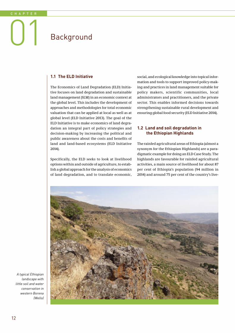
The rainfed agricultural areas of Ethiopia (almost a synonym for the Ethiopian Highlands) are a para-digmatic example for doing an ELD Case Study. The highlands are favourable for rainfed agricultural activities, a main source of livelihood for about 87 per cent of Ethiopia’s population (94 million in 2014) and around 75 per cent of the country’s live-
A typical Ethiopian landscape with
little soil and water conservation in
western Borena (Wello)
A N E L D A S S E S S M E N T
13
stock (60 million units in 1990) (Hurni 1993; Shif-eraw & Holden 1998; Asrat et al. 2004). However, land degradation in this area is considered to be one of the severest cases worldwide (Nyssen et al. 2004). The degree and extent of past and current rates of deforestation and degradation continue to increasingly threaten the food security of the rural poor, with (yet unknown) implications on the national economy (Demeke 2002).
Soil erosion by water is the dominant degradation process and occurs particularly on cropland, with annual soil loss rates on average of 42 tonnes/ha for croplands, and up to 300 tonnes/ha in extreme cases (Hurni 1993). Other degradation processes include intensified runoff from grasslands and related gullying, as well as high soil erosion rates from badlands (heavily degraded lands). The prac-tices of the small-scale farmers are the main ‘cause’ of these processes, although in recent decades they have started taking action alongside government initiatives.
1.3 Contribution to the goals of the ELD Initiative
Spatially explicit information on the degree and extent of both soil degradation processes and investments in SLM technologies in the rainfed agricultural areas of Ethiopia is not yet available. Since such information is crucial for informed deci-sion-making (Pinto-Correia et al. 2006), the ELD Ethiopia Case Study aims to contribute to filling this gap. It focuses on the development of a frame-work for a spatially explicit assessment of land deg-radation (soil erosion by water) and analysis of the costs and benefits of SLM practices. By displaying spatial differences on the status and current pro-cesses of land and soil degradation, on imple-mented and planned SLM technologies and related costs and benefits, potential adaptions of SLM tech-nologies and livelihood options outside of agricul-ture can be economically valued. In this way, the ELD Ethiopia Case Study contributes to the goal of the ELD Initiative of supporting informed decision-making.
In terms of ecosystem services, the proposed assess-ment primarily addresses the productive functions of land and water, particularly through the cultiva-tion of cereals, pulses, and other crops in the ox-plough systems of the rainfed agricultural areas,
which enable a subsistence-based livelihood for a great majority of the Ethiopian peoples. The focus on cropland is justified in view of its importance as a primary cause of soil erosion and degradation. It is further justified due to its considerable share of land cover (about one third of the highland area), and the direct dependence of farming systems on what the soil is able to produce. Grassland is also a major land cover class (for animal feed), which has been included in the land cover component, but is not analysed further in the economic assessment, as soil erosion on grassland is only a fraction of the amount of erosion from cropland when compared on a per unit area basis.
Other ecosystem services like biodiversity, amenity function, or other provisioning services such as water delivery to downstream areas, are not eco-nomically valued here any further. However, for the latter case, the soil erosion and sediment depo-sition analysis will allow for a detailed assessment of potential sediment delivery rates in any river sys-tem originating from the highlands, although their accuracy is based on very little calibration information used here. Furthermore, other ecosys-tem services can be analysed in the future based on the detailed land cover analysis attempted here.
1.4 Location and scope
This study focuses on the parts of Ethiopia where rainfed agriculture is practiced, which covers almost 600,000 km2 = 54 per cent of the country, and 84 per cent of the land is 1000 m/asl and above. Lowland areas below 1000 m/asl were only ana-lysed if they showed rainfed agriculture, although most of it is semi-arid to arid and used mainly by pastoralists who do not normally practice it. As a result, these areas were not analysed in this case study as they are much less affected by human-induced soil degradation than the small-scale farmers in the moist to wet highlands.
The scope of this study is to thus:
(a) Produce a high-resolution land cover map (pixel size: 30 m x 30 m, or 900 m2 per pixel) using 30 land cover classes (Table 2 and Figure 4), from forest to grassland, cropland to settle-ment, and bare land to water body, covering over 660 million pixels for the case study area (599,864 km2);
C H A P T E R 0 1 Background
14
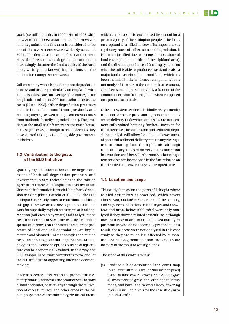
F I G U R E 1
Extent of the ELD Ethiopia Case Study, including nearly 100 per cent of the rainfed agricultural area in Ethiopia
Addis Abeba
!
Agroecological Zones
Dry Berha
Moist Berha
Dry Kolla
Moist Kolla
Wet Kolla
Dry Weyna Dega
Moist Weyna Dega
Wet Weyna Dega
Dry Dega
Moist Dega
Wet Dega
Moist High Dega
Wet High Dega
Moist Wurch
Wet Wurch
Rivers/water bodies
Study area
Main towns
Major roads
National boundary(not authoritative)
0 1 00 200 300km
Agro-ecological zones follow Ethiopian terms, Berha being desert lowlands, Kolla being semi-arid lowlands, Weyna Dega being ecologically favourable humid middle altitudes, Dega and high Dega being coldish to cold highlands, and Wurch being cold alpine meadows (Hurni 1998)
(b) Model the occurrence of soil and water conser-vation structures and fertilizer application on cropland in the study area;
(c) Creation of a pixel based database including the information required to model soil erosion/deposition, to estimate crop production, and to perform a cost-benefit analysis (CBA) of differ-ent management options;
(d) Model soil erosion/deposition using calibra-tion and validation data from research catch-
ments (SCRP 2000) as well as the Abbay (Blue Nile) River Basin;
(e) Estimation of crop production from the soil depth for the current situation (‘business as usual’) and for the coming 30 years assuming different management options, and;
(f) Compute a CBA of the current situation (‘busi-ness as usual’) and of seven additional scenar-ios over 30 years, from ‘business as usual’ to ‘enhanced SLM’, to reduce soil erosion and
A N E L D A S S E S S M E N T
15
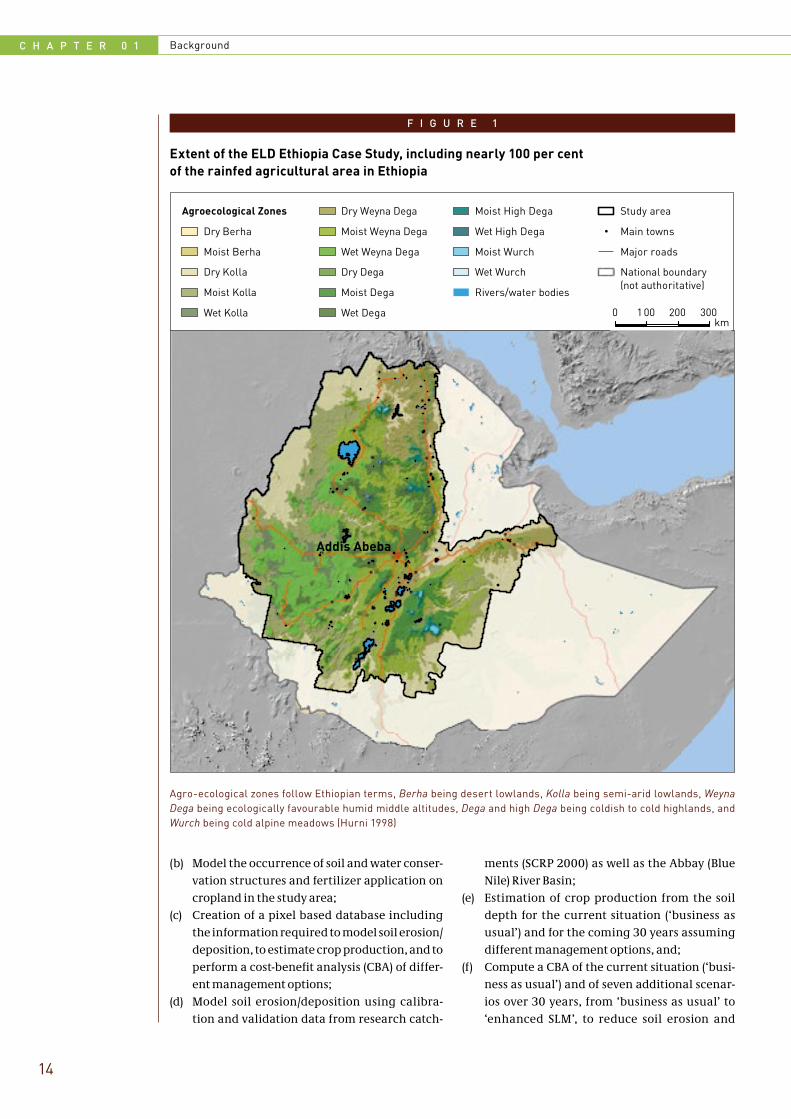
F I G U R E 2
Example of a conserved cropland pixel (30 m x 30 m) and some of the parameters used for the CBA
Runoff, Sediments
Precipitation
Runoff, Sediments
Conservationstructures
Fodder grassplantation
Crop production area
Crop production area
Soil depth
Slope
enhance productivity without agronomic improvements.
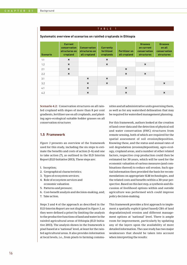
For each rainfed cropland pixel, the parameters shown in Figure 2 were considered. In the study area, there are about 239 million such cropland pixels. About 31 million of these pixels were later on defined by the digital elevation model (DEM) as riverbeds. These pixels were excluded from the analysis because the soil erosion/deposi-tion model would give exorbitant results beyond plausibility. What remained as rainfed agricul-tural areas of Ethiopia were 208 million cropland pixels for which eight scenarios were modelled, described as follows (also see Table 1 for a systemic overview):
Scenario 1.1: Business as usual, i.e., current distri-bution of conservation structures (fanya juu bunds, soil bunds, and stone terraces) and currently ferti-lized croplands, the latter on unconserved flat crop lands as well as on conserved sloping cropland
Scenario 1.2: Business as usual, and planting agro-ecological suitable fodder grasses on current conservation structures
Scenario 2.1: Current distribution of conservation structures with fertilizer use on all rainfed crop-lands
Scenario 2.2: Current distribution of conserva-tion structures with fertilizer use on all rainfed croplands, and planting agro-ecological suitable fodder grasses on current conservation structures
Scenario 3.1: Conservation structures on all rain-fed croplands with slopes of more than 8 per cent gradients, and current distribution of fertilizer use on flat lands as well as on currently conserved crop-lands
Scenario 3.2: Conservation structures on all rain-fed croplands with slopes of more than 8 per cent gradients, and current distribution of fertilizer use on flat lands as well as on currently conserved crop-lands, and planting agro-ecological suitable fod-der grasses on all conservation structures
Scenario 4.1: Conservation structures on all rain-fed cropland with slopes of more than 8 per cent gradients and fertilizer use on all croplands
C H A P T E R 0 1 Background
16
Scenario 4.2: Conservation structures on all rain-fed cropland with slopes of more than 8 per cent gradients, fertilizer use on all croplands, and plant-ing agro-ecological suitable fodder grasses on all conservation structures
1.5 Framework
Figure 3 presents an overview of the framework used for this study, including the six steps to esti-mate the benefits and costs of action (1–6) and one to take action (7), as outlined in the ELD Interim Report (ELD Initiative 2013). These steps are:
1. Inception; 2. Geographical characteristics; 3. Types of ecosystem services; 4. Role of ecosystem services and
economic valuation5. Patterns and pressure;6. Cost-benefit analysis and decision-making, and; 7. Take action.
Steps 3 and 4 of the approach as described in the ELD Interim Report are not displayed in Figure 3, as they were defined a priori by limiting the analysis to the productive functions of land and water in the rainfed agricultural areas of Ethiopia (ELD Initia-tive 2013). The analysis shown in the framework is pixel based at a ‘national’ level, at least for the rain-fed agricultural areas. It also provides information at local levels, i.e., from pixels to farming commu-
nities and all administrative units governing them, as well as for any watershed delineation that may be required for watershed management planning.
For this framework, authors looked at the creation of land cover data and the detection of physical soil and water conservation (SWC) structures from remote sensing, both of which are required for the spatial assessment of soil erosion/deposition. Knowing these, and the status and annual rates of soil degradation (erosion/deposition), agro-ecol-ogy, cropland areas, and a number of other related factors, respective crop production could then be estimated for 30 years, which will be used for the economic valuation of various measures (and com-binations thereof) to reduce soil erosion. Such spa-tial information then provided the basis for recom-mendations on appropriate SLM technologies, and the related costs and benefits within a 30-year per-spective. Based on this last step, a synthesis and dis-cussion of livelihood options within and outside agriculture was performed wich could improve policy decision-making.
This framework provides a first approach to imple-ment a spatially explicit (pixel based) CBA of land degradation/soil erosion and different manage-ment options at ‘national’ level. There is ample room for improvement, particularly by updating any of the layers upon the availability of more detailed information. The case study has two major weaknesses that should be taken into account when interpreting the results:
T A B L E 1
Systematic overview of scenarios on rainfed croplands in Ethiopia
Scenario
Current conservation structures on
cropland
Conservation structures on all cropland
Currently fertilized croplands
Fertilizer on all cropland
Grasses on current
conservation structures
Grasses on all
conservation structures
1.1 l l
1.2 l l l
2.1 l l
2.2 l l l
3.1 l l
3.2 l l l
4.1 l l
4.2 l l l

A N E L D A S S E S S M E N T
17
❚❚ The distribution of current soil conservation structures is based on expert knowledge about current efforts invested by regions since the 1970s, improved by some modelling of their most likely distribution using proximity to set-tlements and roads, steepness of terrain, and cropland (the study’s initial approach using remote sensing information for detecting such structures automatically had failed).
❚❚ The erosion/deposition model could be cali-brated and validated for small catchments for which long-term data existed, such as in the Soil Conservation Research Programme (SCRP) research catchments. However, the application of the model to larger basins had to be done using just one piece of information from the
Abbay (Blue Nile) Basin that may date as far back as 50 years, namely an annual sediment deliv-ery of at least 300 million tonnes for a major part of the basin (Abdelsalam 2008).
In general, however, authors are very pleased with the outcomes of this study, which can be adapted (if more detailed information becomes available) to small areas, such as catchments from a few hec-tares to square kilometres in seize, but also to other regions world-wide for which similar conditions exist.
The following chapter presents the methodologi-cal components required for the implementation of this framework.
F I G U R E 3
Framework for the assessment and economic valuation of soil degradation and various SLM practices in the rainfed agricultural area of Ethiopia and related ELD step(1 to 9 are steps in the assessment; [1] to [7] refer to the ELD Initiative [see text]).
1: Land cover Precipitation Terrain Soil Conservation structures [1; 2]
2: Soil erosion / deposition [5]
3: Soil depth - yearly erosion + yearly deposition = Soil depths for the next 30 years [5]
4: Definition of crop yield - soil depth relationships for the different agroecological zones [5]
5: Calculation of crop yields for the next 30 years (crop yield benefits) [5]
6: Calculation of additional benefits (e.g., fodder grass cultivation on terraces) [6]
7: Definition of costs (structure building / maintenance; costs related to management options (e.g. fertilizer costs)) [6]
8: CBA of structural measures / different management options for the next 30 years [6]
9: Assessment of the costs of land degradation and the economic validity ofstructural measures and different management options at pixel level
[6; 7]
[6; 7]
C H A P T E R
02
18
Components of the ELD Ethiopia Case Study
A series of base layers need to be created in order to model soil erosion/deposition and to perform a CBA of different agricultural management options. Authors used remote sensing (e.g., land cover data) and quite often also GIS modelling (e.g., for approx-imating the distribution of the currently existing conservation structures, application of fertilizer, or crop prices). This helped in translating the expert knowledge and statistical data into spatial infor-mation. The methodologies, approaches, assump-tions used to create these base layers, and main results from each component are presented in the following chapters.
2.1 Component 1: Land cover mapping
2.1.1 Background and scope
For this study, up-to-date and detailed land cover information at a 30 m pixel resolution was required. Such information is available in terms of resolution and detail, but only at local case study scales scat-tered over the Ethiopian Highlands. Only a few datasets exist at the national scale, namely those produced by the Ethiopian Highlands Reclamation Study in the 1980s, the Woody Biomass Inventory and Strategic Planning Project in the 1990s, and a land use land cover (LULC) map developed by FAO/LUPRD in the 1980s. However, these are all out-dated and did not show sufficient detail for this study. In order to assess the economics of land deg-radation, this study required land cover data at a scale that represents the local level land cover char-acteristics while still covering the rainfed agricul-tural areas of Ethiopia. Consequently, authors needed to produce a land cover dataset to suit these requirements.
A major challenge in mapping land cover from remote sensing imagery in Ethiopia was the com-plex biophysical and socio-cultural setting. The long history of smallholder cultivation in many parts of the highlands has resulted in a heterogene-
ous landscape consisting of a mix of small patches of land cover classes. These land cover mosaics also vary in terms of composition and frequency of occurrence in the wider landscape. There is also heterogeneity in terms of land cover classes and their composition between the agro-ecological zones, related to varying cultural practices, farm-ing systems, precipitation regimes, and last but not least, the often rugged terrain.
There are additional challenges related to the acquisition dates and spectral and spatial resolu-tion of remotely sensed imagery. Firstly, the rugged terrain heavily affects the spectral reflectance cap-tured by satellites (Dorren et al. 2003). Depending on the gradient of the slope, the same land cover can appear completely different in the remote sens-ing imagery and can be easily confused with other land cover classes. Secondly, the acquisition dates of images with low or no cloud cover are mostly during the dry season, but during this time remote sensing specialists are confronted with the prob-lem of land cover (e.g., grasslands and croplands) having very similar spectral reflectance, which is also easily confused.
As a result, commonly applied remote sensing clas-sification approaches (e.g., supervised classifica-tion of a whole image after the collection of few training and verification areas) do not allow for an accurate classification and often under- or overes-timate certain land cover features. To derive a land cover dataset that accurately represents the hetero-geneity of the Ethiopian landscape, contextual approaches were required that considered the complex biophysical and socio-cultural setting so that the local settings could be properly captured.
2.1.2 Data and methodology
The following sections describe the remote sensing data used to derive land cover, selection of land cover classes, and the development of classification approaches and methodologies.

A N E L D A S S E S S M E N T
19
Remote sensing imagery
In terms of image availability and aspired spatial resolution for this study, Landsat data (30 m pixels) was found to be appropriate. With this data, the final map can be considered reliable for scales between 1:50,000 and 1:100,000. Considering the long time-series of Landsat data, as well as the con-tinuation of the Landsat mission (Landsat 8 was launched in spring 2013), an approach developed with Landsat data allows for a repetition of the land cover mapping targeting different time steps, also in the future. Additionally, Landsat images are pro-vided for free (e.g., earthexplorer.usgs.gov). In this study, Landsat Thematic Mapper data covering the period from 2008–2011 was used. Due to cloud and haze cover, it was not possible to use images from only one specific year.
Selection of land cover classes
The Landsat images chosen for the classification were thoroughly assessed in order to identify the features that could be reasonably mapped and extracted from the imagery. Authors assumed that the appropriate mapping detail should at least involve features showing a 150 m x 150 m extent. Based on this, and considering the objectives of the study, a classification scheme involving 30 distinct land cover classes was then defined.
Approach and methodology
In order to deal with the complexity and heteroge-neity of the land cover, the following approach was applied to obtain a dataset that covers the whole study area while still capturing the local character-istics of the complex Ethiopian rainfed agricultural landscape:
❚❚ Deriving Homogenous Image Classification Units (HICUs) that subdivided each Landsat image into smaller units where similar land cover mosaics occur was found to be a suitable classification approach. HICU development was done using multiple information sources such as altitude, terrain, farming system, rainfall pattern, and soil. This approach resulted in a varying amount of HICUs within a Landsat image, depending on the location and land-scapes. In areas with relatively less heterogene-ity, e.g., in flat highland plateaux like Central Gojam, Central Oromia, Gambela, and Benis-
hangul-Gumuz regions, 20–30 HICUs per Land-sat image where sufficient. In more heteroge-neous landscapes, e.g., the northern mountain-ous areas like Wello, Gonder and Tigray, up to 100–200 HICUs per Landsat image were deline-ated.
❚❚ The next step of the LULC mapping consisted of identifying the dominant and subordinate land cover features for each HICU, hereto after referred as majority and minority classes. For each HICU this involved grouping land features into minority and majority classes based on the occurrence, dominance, and distribution of the land features. While the classes varied for each HICU, they usually included forests (church for-ests, plantation forests, protected high forests), homestead plantations, irrigated landscapes, large-scale investments, settlements, and ponds and small lakes. Depending on the loca-tion of the HICU in the study area, forests could be either a majority class (covering a large share of the HICU) or a minority class, while the other aforementioned land features usually were a minority class (covering small areas, scattered within the HICU). Different approaches like manual digitizing, edge enhancement, and NDVI thresholding were used to extract the majority and/or minority classes from the imagery. The extracted classes were combined and areas of their occurrence masked within each Landsat image, so that they would not dis-tort the further classification process.
❚❚ For each HICU, an unsupervised classification was run (ISODATA cluster algorithm) and 20–40 unsupervised classes generated. These classes were then checked against high resolution Google Earth imagery and labelled by experts with experience in the areas where the images where located. In case the unsupervised classi-fication within a HICU did not provide suffi-ciently detailed classes, the amount of unsuper-vised classes was increased, and if the classifica-tion was still not satisfactory, the HICU was further subdivided.
❚❚ Merging of the HICUs and the Landsat images, and crosschecking of assigned classes was done in a mutual effort by experts. This was neces-sary, as for example, at some of the image boundaries, differences in the attributed land cover classes could be observed. These areas
C H A P T E R 0 2 Components of the ELD Ethiopia Case Study
20
were relabelled after coming to a consensus among the land cover experts.
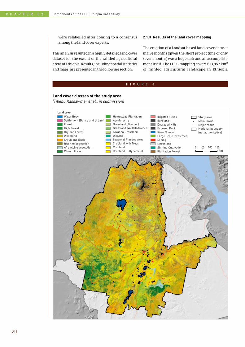
This analysis resulted in a highly detailed land cover dataset for the extent of the rainfed agricultural areas of Ethiopia. Results, including spatial statistics and maps, are presented in the following section.
2.1.3 Results of the land cover mapping
The creation of a Landsat-based land cover dataset in five months (given the short project time of only seven months) was a huge task and an accomplish-ment itself. The LULC mapping covers 613,957 km2
of rainfed agricultural landscape in Ethiopia
F I G U R E 4
Land cover classes of the study area(Tibebu Kassawmar et al., in submission)
Land cover
!
0 50 100 150km
Water BodySettlement (Dense and Urban)ForestHigh ForestDryland ForestWoodlandShrub and BushRiverine VegetationAfro Alpine VegetationChurch Forest
Homestead PlantationAgroforestryGrassland (Drained)Grassland (Wet/Undrained)Savanna GrasslandWetlandSeasonal Flooded AreaCropland with TreesCroplandCropland (Hilly Terrain)
Irrigated FieldsBarelandDegraded HillsExposed RockRiver CourseLarge Scale InvestmentMiningMarshlandShifting CultivationPlantation Forest
Study areaMain townsMajor roadsNational boundary(not authoritative)
A N E L D A S S E S S M E N T
21
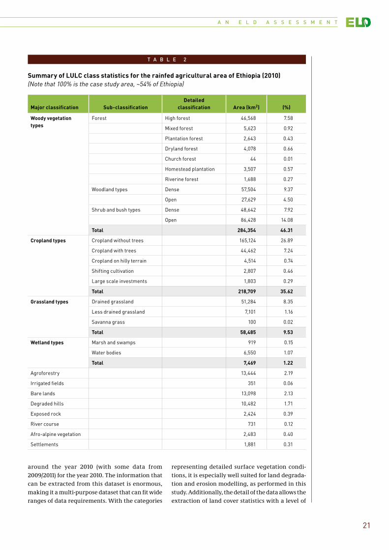
around the year 2010 (with some data from 2009/2011) for the year 2010. The information that can be extracted from this dataset is enormous, making it a multi-purpose dataset that can fit wide ranges of data requirements. With the categories
representing detailed surface vegetation condi-tions, it is especially well suited for land degrada-tion and erosion modelling, as performed in this study. Additionally, the detail of the data allows the extraction of land cover statistics with a level of
T A B L E 2
Summary of LULC class statistics for the rainfed agricultural area of Ethiopia (2010)(Note that 100% is the case study area, ~54% of Ethiopia)
Major classification Sub-classificationDetailed
classification Area (km2) (%)
Woody vegetation types
Forest High forest 46,568 7.58
Mixed forest 5,623 0.92
Plantation forest 2,643 0.43
Dryland forest 4,078 0.66
Church forest 44 0.01
Homestead plantation 3,507 0.57
Riverine forest 1,688 0.27
Woodland types Dense 57,504 9.37
Open 27,629 4.50
Shrub and bush types Dense 48,642 7.92
Open 86,428 14.08
Total 284,354 46.31
Cropland types Cropland without trees 165,124 26.89
Cropland with trees 44,462 7.24
Cropland on hilly terrain 4,514 0.74
Shifting cultivation 2,807 0.46
Large scale investments 1,803 0.29
Total 218,709 35.62
Grassland types Drained grassland 51,284 8.35
Less drained grassland 7,101 1.16
Savanna grass 100 0.02
Total 58,485 9.53
Wetland types Marsh and swamps 919 0.15
Water bodies 6,550 1.07
Total 7,469 1.22
Agroforestry 13,444 2.19
Irrigated fields 351 0.06
Bare lands 13,098 2.13
Degraded hills 10,482 1.71
Exposed rock 2,424 0.39
River course 731 0.12
Afro-alpine vegetation 2,483 0.40
Settlements 1,881 0.31
C H A P T E R 0 2 Components of the ELD Ethiopia Case Study
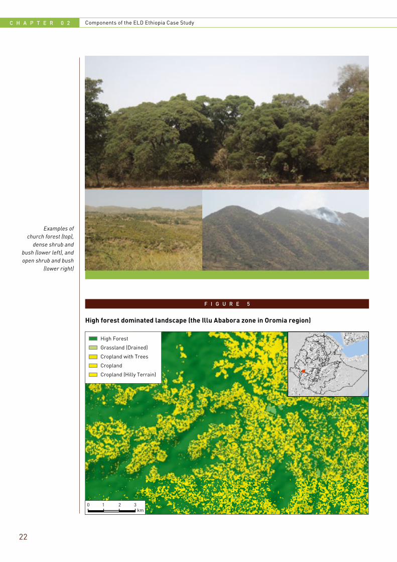
22
Examples of church forest (top),
dense shrub and bush (lower left), and open shrub and bush
(lower right)
F I G U R E 5
High forest dominated landscape (the Illu Ababora zone in Oromia region)
0 1 2 3km
High Forest
Grassland (Drained)
Cropland with Trees
Cropland
Cropland (Hilly Terrain)
A N E L D A S S E S S M E N T
23
accuracy that was not previously available. Some of the statistical findings and highlights related to the land cover data are provided further on.
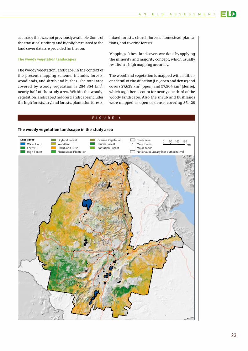
The woody vegetation landscapes
The woody vegetation landscape, in the context of the present mapping scheme, includes forests, woodlands, and shrub and bushes. The total area covered by woody vegetation is 284,354 km2, nearly half of the study area. Within the woody-vegetation landscape, the forest landscape includes the high forests, dryland forests, plantation forests,
mixed forests, church forests, homestead planta-tions, and riverine forests.
Mapping of these land covers was done by applying the minority and majority concept, which usually results in a high mapping accuracy.
The woodland vegetation is mapped with a differ-ent detail of classification (i.e., open and dense) and covers 27,629 km2 (open) and 57,504 km2 (dense), which together account for nearly one third of the woody landscape. Also the shrub and bushlands were mapped as open or dense, covering 86,428
F I G U R E 6
The woody vegetation landscape in the study area
km!
Land cover
Water BodyForestHigh Forest
Dryland ForestWoodlandShrub and BushHomestead Plantation
Riverine VegetationChurch ForestPlantation Forest
Study areaMain townsMajor roadsNational boundary (not authoritative)
0 50 100 150
C H A P T E R 0 2 Components of the ELD Ethiopia Case Study
24
km2 (open) and 48,642 km2 (dense), accounting together for nearly half of the woody landscape.
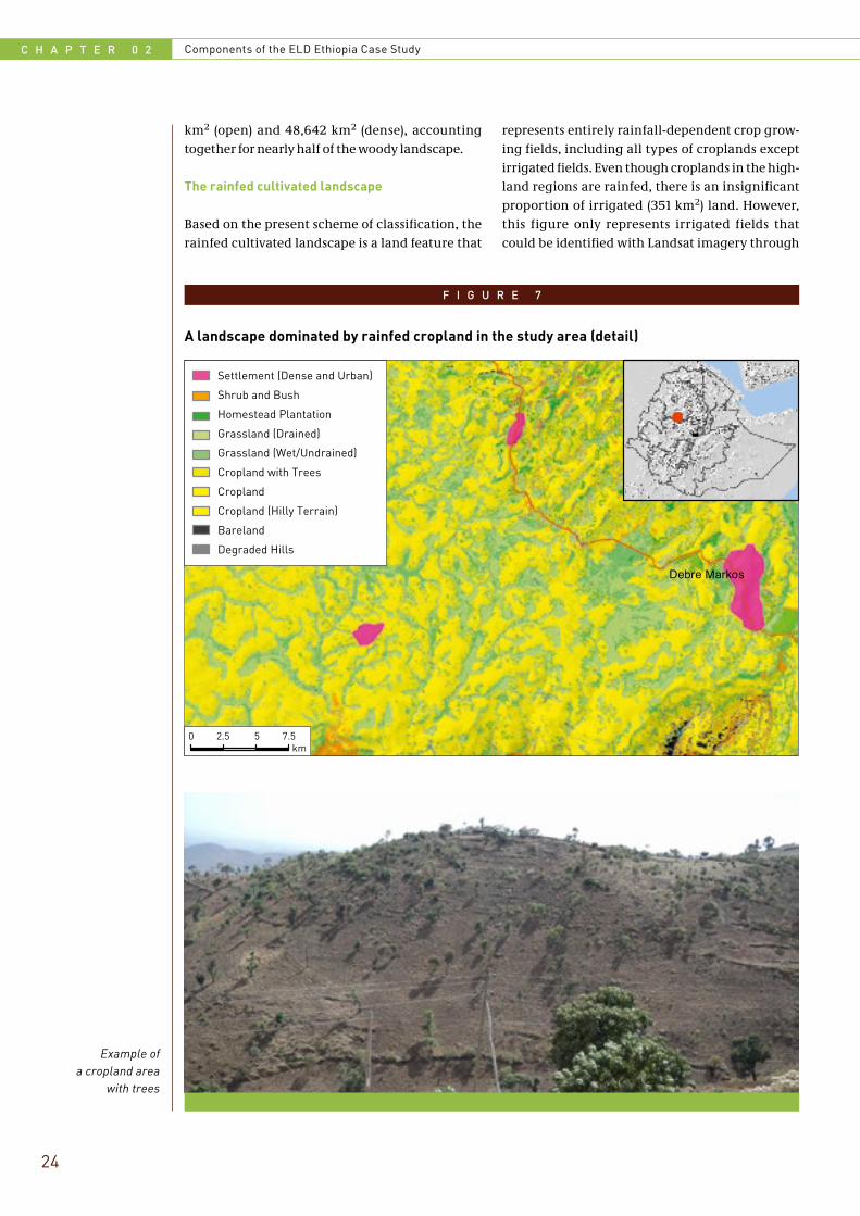
The rainfed cultivated landscape
Based on the present scheme of classification, the rainfed cultivated landscape is a land feature that
represents entirely rainfall-dependent crop grow-ing fields, including all types of croplands except irrigated fields. Even though croplands in the high-land regions are rainfed, there is an insignificant proportion of irrigated (351 km2) land. However, this figure only represents irrigated fields that could be identified with Landsat imagery through
F I G U R E 7
A landscape dominated by rainfed cropland in the study area (detail)
Debre Markos
km
Settlement (Dense and Urban)
Shrub and Bush
Homestead Plantation
Grassland (Drained)
Grassland (Wet/Undrained)
Cropland with Trees
Cropland
Cropland (Hilly Terrain)
Bareland
Degraded Hills
0 2.5 5 7.5
Example of a cropland area
with trees
A N E L D A S S E S S M E N T
25
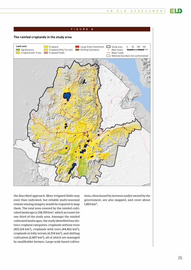
the described approach. More irrigated fields may exist than indicated, but reliable multi-seasonal remote sensing imagery would be required to map them. The total area covered by the rainfed culti-vated landscape is 218,709 km2, which accounts for one third of the study area. Amongst the rainfed cultivated landscapes, the study identified four dis-tinct cropland categories: croplands without trees (165,124 km2), croplands with trees (44,462 km2), croplands in hilly terrain (4,514 km2), and shifting cultivation (2,807 km2), all of which are managed by smallholder farmers. Large-scale based cultiva-
tions, often leased by investors and/or owned by the government, are also mapped, and cover about 1,803 km2.
F I G U R E 8
The rainfed croplands in the study area
0 50 100 150km!
Land cover
AgroforestryCropland with Trees
CroplandCropland (Hilly Terrain)Irrigated Fields
Large Scale InvestmentShifting Cultivation
Study areaMain townsMajor roadsNational boundary (not authoritative)
C H A P T E R 0 2 Components of the ELD Ethiopia Case Study
26
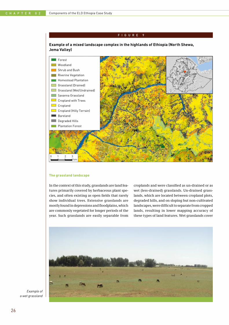
The grassland landscape
In the context of this study, grasslands are land fea-tures primarily covered by herbaceous plant spe-cies, and often existing as open fields that rarely show individual trees. Extensive grasslands are mostly found in depressions and floodplains, which are commonly vegetated for longer periods of the year. Such grasslands are easily separable from
croplands and were classified as un-drained or as wet (less-drained) grasslands. Un-drained grass-lands, which are located between cropland plots, degraded hills, and on sloping but non-cultivated landscapes, were difficult to separate from cropped lands, resulting in lower mapping accuracy of these types of land features. Wet grasslands cover
F I G U R E 9
Example of a mixed landscape complex in the highlands of Ethiopia (North Shewa, Jema Valley)
0 1 2 3km
Forest
Woodland
Shrub and Bush
Riverine Vegetation
Homestead Plantation
Grassland (Drained)
Grassland (Wet/Undrained)
Savanna Grassland
Cropland with Trees
Cropland
Cropland (Hilly Terrain)
Bareland
Degraded Hills
Plantation Forest
Example of a wet grassland
A N E L D A S S E S S M E N T
27
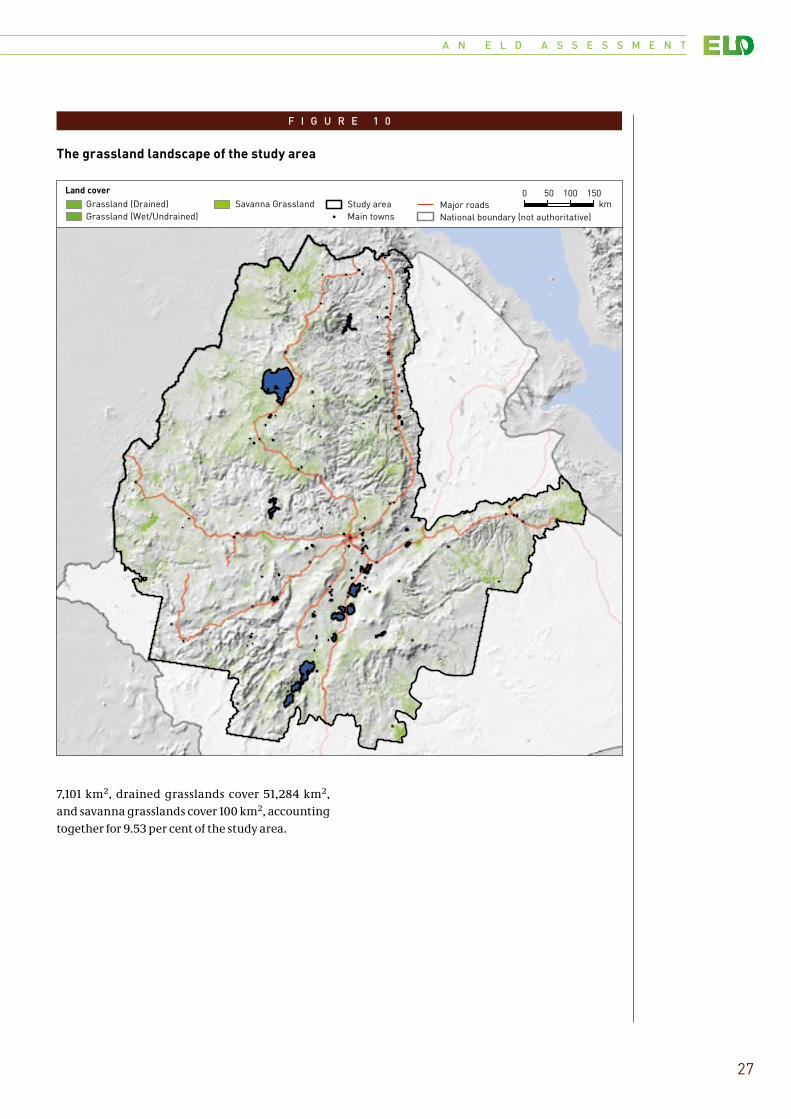
F I G U R E 1 0
The grassland landscape of the study area
km!
Land coverGrassland (Drained)Grassland (Wet/Undrained)
Savanna Grassland Study areaMain towns
Major roadsNational boundary (not authoritative)
0 50 100 150
7,101 km2, drained grasslands cover 51,284 km2, and savanna grasslands cover 100 km2, accounting together for 9.53 per cent of the study area.
C H A P T E R 0 2 Components of the ELD Ethiopia Case Study
28
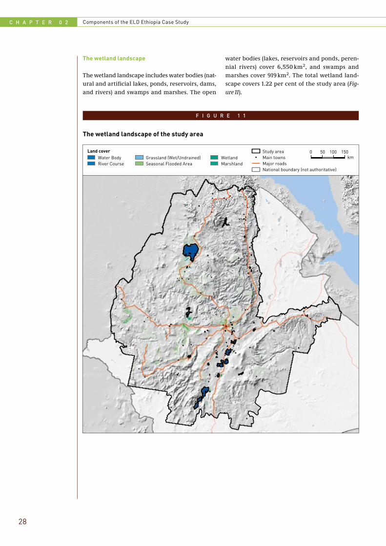
The wetland landscape
The wetland landscape includes water bodies (nat-ural and artificial lakes, ponds, reservoirs, dams, and rivers) and swamps and marshes. The open
water bodies (lakes, reservoirs and ponds, peren-nial rivers) cover 6,550 km2, and swamps and marshes cover 919 km2. The total wetland land-scape covers 1.22 per cent of the study area (Fig-ure 11).
F I G U R E 1 1
The wetland landscape of the study area
km!
Land coverWater BodyRiver Course
Grassland (Wet/Undrained)Seasonal Flooded Area
WetlandMarshland
Study areaMain townsMajor roadsNational boundary (not authoritative)
0 50 100 150
A N E L D A S S E S S M E N T
29
AgroforestryAgroforestry landscapes are found extensively in the Gedio, Gurage, Jima Zone, and other southern regions. They are dominated by trees with coffee, inset (false banana), chat (khat, a leaf drug), mango, and avocado. These land features cover 13,444 km2
and accounts for 2.19 per cent of the study area. Bare landsIn the context of this study, bare lands are barren surfaces where vegetation hardly exists. They are non-vegetated and non-productive landscapes found largely along riversides, quarry and con-struction sites, riverbeds, and degraded lands. The total area covered by these types of land features is 13,098 km2, and accounts for 2.13 per cent of the study area.
Exposed rockIn the northern part of the country there are areas where the degradation process reaches to a stage where the parent material surfaces. The total area mapped as exposed rock covers 2,424 km2, and accounts for 0.37 per cent of the study area.
River coursesWith the 30 m resolution of the Landsat data and the applied mapping approach, most of the river courses could be mapped unless dense riverine
vegetation hindered the detection of water. The total area of the river courses covers 731 km2.
Afro-alpine vegetationThere is a unique altitudinal range where these land features exist, simplifying the mapping of afro-alpine vegetation. Commonly afro-alpine regions are covered by herbaceous plant species (rarely by shrub/bush or Ericaceous trees) at alti-tudes above about 3,400 m/asl. The total area cov-ered by these land features is 2,483 km2, which accounts for 0.40 per cent of the study area.
SettlementsSettlement areas (mainly urban centres as well as clustered and dense rural settlements) have been identified and mapped. The total area covered by settlements is 1,881 km2, which accounts for 0.31 per cent of the study area.
OthersLand features other than those mentioned above (e.g., mining and quarry sites, area covered by inva-sive species, etc.) are insignificant in terms of area coverage, but were also considered in the mapping process. The total area covered by such land fea-tures is 47 km2, which accounts for 0.01 per cent of the study area.
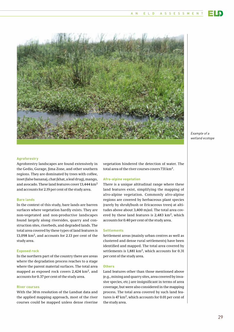
Example of a wetland ecotope
C H A P T E R 0 2 Components of the ELD Ethiopia Case Study
30
2.1.4 Conclusion and recommendations
The main methodological approach implemented to map this complex landscapes at the required scale was the majority and minority concept of landscape segregation that translated into the HICU-based mapping. This approach enabled authors to capitalize on the unprecedented quali-ties that exist in the satellite images used. The employment of such an ‘exclusion-based’ approach (i.e., sub-setting of the image and gradually reduc-ing the minorities/majorities) can be considered as a breakthrough in deriving important land cover information in heterogeneous landscapes, such as this rainfed agricultural area of Ethiopia.
The present study has achieved the extraction of 50 distinct land features from medium (30 m x 30 m pixels) resolution satellite images. Only for simplic-ity’s sake were all of these classes not considered in the maps and statistics. However, the digital data contains all 50 classes as independently mapped land features. While a pixel based accuracy assess-ment of the land cover data could not yet be pro-duced due to time restrictions, the comparison with Google Earth high resolution imagery shows satisfactory results. Even though the accuracy of the different land cover classes can vary between classes and regions, the comparison with other sub-national (regional) and national land cover datasets clearly shows a significant improvement of this dataset.
2.2 Component 2: Conservation structure mapping
2.2.1 Detection of conservation structures from high resolution satellite images
Conservation structure mapping approach
Authors attempted to apply an automated model that can map physical soil and water conservation structures (fanya juu bunds, soil bunds, and stone terraces) on croplands of the Ethiopian Highlands (Mekuriaw 2014). The model was developed using the very high spatial resolution imagery (less than 1 m) obtained from Google Earth, field verification, image analyst software (i.e., ArcGIS, ERDAS IMAG-INE, and SDC Morphology Toolbox for MATLAB), and statistical analyses.
The mapping of the structures was performed using the following procedures: first, a high-pass spatial filter algorithm was applied to the target image to detect linear features. Second, morpho-logical processing (e.g., opening, thinning, clos-ing, and skeletonisation using structuring ele-ments) was used to remove unwanted linear fea-tures. Third, the raster format of linear features was vectorised. Fourth, the target area was split into hectares to get land units of similar size. Fifth, the vectorised linear features were split per hec-tare, and each line was then classified according to its compass direction. Sixth, the sum of all vector lengths per class of direction per hectare was cal-culated. Finally, the direction class with the great-est length was selected from each hectare to pre-dict the physical SWC structures.
This model was developed and calibrated within a PhD study – readers can refer to Mekuriaw (2014) for more information on the approach and methodol-ogy, and obtained results.
Results of the conservation structure mapping within this study
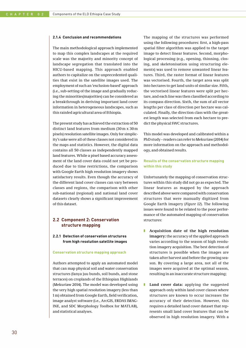
Unfortunately the mapping of conservation struc-tures within this study did not go as expected. The linear features as mapped by the approach described above were compared with conservation structures that were manually digitized from Google Earth imagery (Figure 12). The following issues were found to be related to the poor perfor-mance of the automated mapping of conservation structures:
❚❚ Acquisition date of the high resolution imagery: the accuracy of the applied approach varies according to the season of high resolu-tion imagery acquisition. The best detection of structures is possible when the images are taken after harvest and before the growing sea-son. By covering a large area, not all of the images were acquired at the optimal season, resulting in an inaccurate structure mapping;
❚❚ Land cover data: applying the suggested approach only within land cover classes where structures are known to occur increases the accuracy of their detection. However, this requires a detailed land cover dataset that rep-resents small land cover features that can be observed in high resolution imagery. With a
A N E L D A S S E S S M E N T
31
resolution of 30 m, the difference in resolution was too big to allow for an accurate detection of structures in this study, and;
❚❚ Computer resources: working with high reso-lution imagery increases computational time heavily. Within the project time, it was not pos-sible to further invest on adaptions of the auto-mated structure mapping approach for over-coming other aforementioned limitations.
With the remote sensing approach of mapping existing conservation structures not able to pro-vide the required information, authors had to find another way of obtaining information on their dis-tribution. This is described in the following sec-tions.
2.2.2 Distribution of current conservation structures
To model the current distribution of existing con-servation structures, an expert-based approach was applied that first defined the amount in each administrative zone, and then used a combination of spatial proxies to model the locations where they occur.
Definition of occurrence of conservation structures
To define the occurrence of conservation struc-tures, five experts with vast field experience defined which land cover classes with conservation structures exist (besides cropland, in some of the zones conservation structures also exist on bush-land, grassland, and degraded hills), for each administrative zone. Then, the share of these land
F I G U R E 1 2
Comparison of manually digitized structures (green) and automatically extracted structures (red)
km
Automatically extracted structures
Manually digitized stuctures
Watershed of Maybar (based on ASTERDEM)
0 0.25 0.5
C H A P T E R 0 2 Components of the ELD Ethiopia Case Study
32
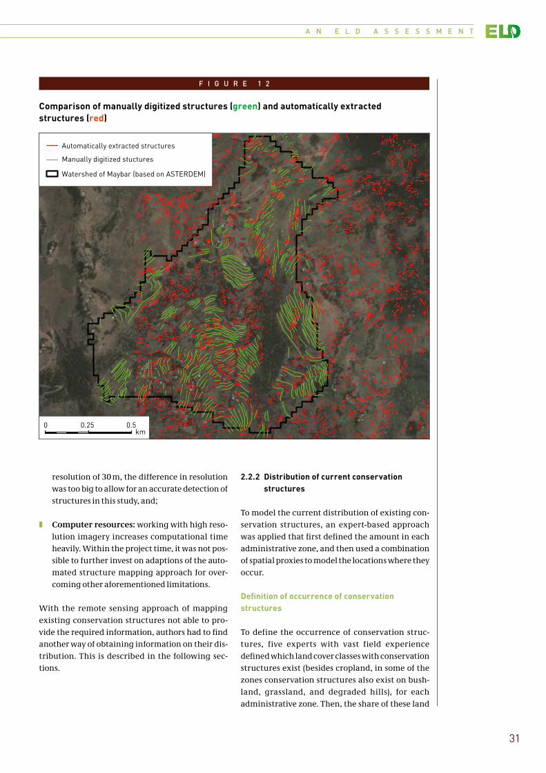
F I G U R E 1 3
The share of the existing conservation structures by land cover classes (For most of the zones the structures only occur on croplands. However, in central Tigray, Eastern Tigray, South Tigray, North Wello and South Wello, structures exist on cropland, bushland, grassland, and degraded hills)
!
Conserved land cover (%)
‹ = 1
1 - 5
5 - 20
20 - 40
40 - 75
Study area
Main towns
Major roads
Rivers/water bodies
National boundary (not authoritative)
cover classes conserved for each zone was defined (see Figure 13).
Spatial proxies and their combination to model conservation structures
Together with the SWC experts, authors selected spatial proxies from the datasets available in Ethio-GIS II that could serve to model the distribution of conservation structures at the pixel level. Three datasets were identified that could be used to approximate the spatial distribution of the struc-tures: land cover, slope, and accessibility:
Land cover: for each administrative zone the land cover classes within which conservation structures exist were defined. In Central Tigray, Eastern Tig-ray, South Tigray, North Wello, and South Wello,
conservation structures occur on cropland, but also in areas with shrubs and bushes, grasslands, and degraded hills. In the other administrative zones, conservation structures only exist in crop-lands. Figure 13 shows the share of these land cover classes that contain conservation structures.
Slope: within the defined land cover classes, the distribution of the conservation structures also relates to slope. Seven slope classes that affect the occurrence of conservation structures were defined: 1) 0–2 per cent; 2) 2–5 per cent; 3) 5–8 per cent; 4) 8–16 per cent; 5) 16–30 per cent; 6) 30–45 per cent, and; 7) >45 per cent. The occurrence of conservation structures within each of these slope classes depends on the total amount of terraces that occur within each administrative zone. Ter-races are found more commonly on hillsides with
A N E L D A S S E S S M E N T
33
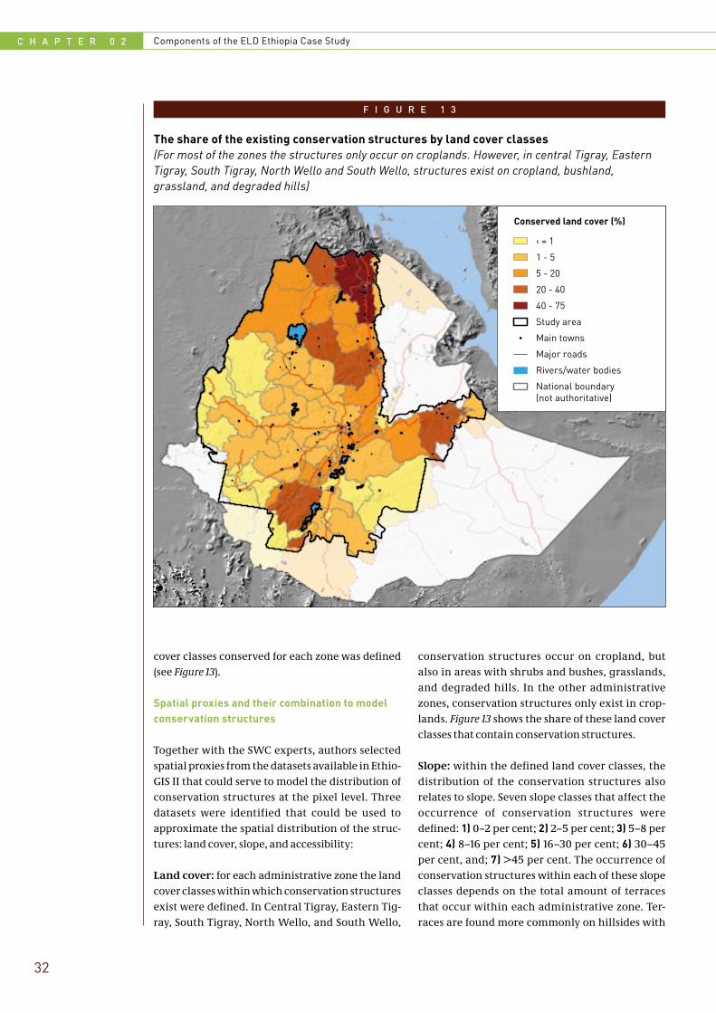
F I G U R E 1 4
Village accessibility map(Colours indicate travel time in minutes from any location to the next settlement, assuming that the fastest means of transportation is chosen)
!
Village accessibilitytravel time in minutes
0 - 15
15 - 30
30 - 60
60 - 120
120 - 180
180 - 240
240 - 852
Study area
Main towns
Major roads
Rivers/water bodies
National boundary(not authoritative)
slopes from 16–30 per cent, but with increasing structure occurrence, they can also be found (in order of more common occurrences) on slopes from 30–45 per cent, then 8–16 per cent, >45 per cent, and 5–8 per cent. The study assumed that struc-tures did not occur in areas with slopes <5 per cent.
Village accessibility: using just land cover classes and slope classes did not allow authors to model the distribution of the conservation structures satis-factorily. An additional spatial proxy was needed that would represent areas where policies and development projects focusing on the construction of conservation structures are more likely to be implemented. A village accessibility layer, indicat-ing how much travel time in minutes is required to reach the closest settlement (assuming the fastest possible means of transportation) for each pixel was found to be a good proxy.
Village accessibility was calculated following the approach described by Heinimann (2006), which includes information on land cover, slope, road data, rivers, and village points to estimate, for each pixel, the travel time to the closest village point assuming that the fastest means of land-based transportation (e.g., travelling by car on roads and on foot for other land cover classes) is used. Figure 14 shows the village accessibility calculated for the study area. This continuous layer was also reclassi-fied into seven accessibility zones with class breaks. Authors assumed that conservation structures are more likely to occur in more accessible areas (less travel time from villages).
To model conservation structure distribution within the study area, a spatial combination of the different proxies was performed: land cover classes with conservation structures were combined with
C H A P T E R 0 2 Components of the ELD Ethiopia Case Study
34
the slope and village accessibility classes. This resulted in a dataset where each pixel had the fol-lowing information: land cover class, grade of slope class, and travel time to the next settlement class. This information was summarized for each administrative zone, and revealed which class combinations occurred within each zone, as well as the area covered by each occurring combina-tions. The conservation structures were then dis-tributed within these class combinations until the amount of conserved area within the administra-tive zone as defined by the experts was reached. Conservation structures were first assumed to occur on more sloping lands (8 per cent and steeper) and close to settlements/roads (rather accessible). If only few conservation structures exist within a zone, the terrace distribution model assumed that the terraces occur on steep slopes only and rather close to the village. The more con-servation structures exist within a zone, terraces were also assumed to be on less sloping land and
also further away from the villages (less accessi-ble).
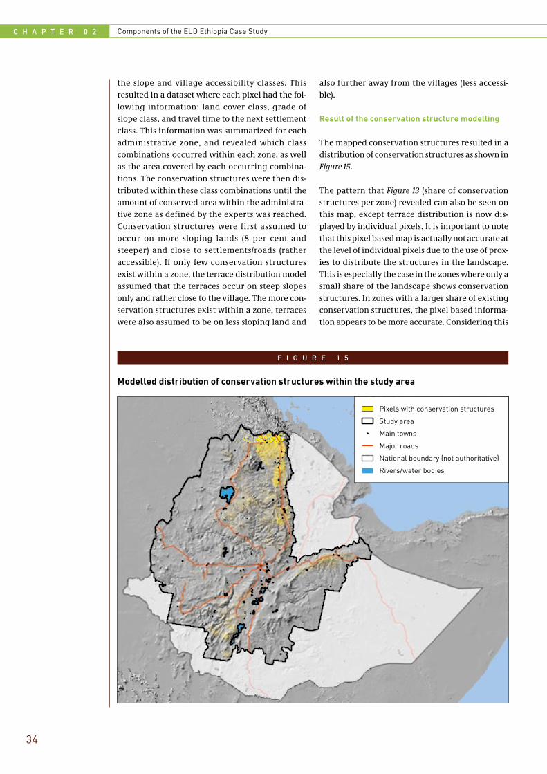
Result of the conservation structure modelling
The mapped conservation structures resulted in a distribution of conservation structures as shown in Figure 15.
The pattern that Figure 13 (share of conservation structures per zone) revealed can also be seen on this map, except terrace distribution is now dis-played by individual pixels. It is important to note that this pixel based map is actually not accurate at the level of individual pixels due to the use of prox-ies to distribute the structures in the landscape. This is especially the case in the zones where only a small share of the landscape shows conservation structures. In zones with a larger share of existing conservation structures, the pixel based informa-tion appears to be more accurate. Considering this
F I G U R E 1 5
Modelled distribution of conservation structures within the study area
!
Pixels with conservation structures
Study area
Main towns
Major roads
National boundary (not authoritative)
Rivers/water bodies

A N E L D A S S E S S M E N T
35
level of generalization, the information provided by this model can be assumed to be accurate from wereda/zone level and upwards. This limitation should be kept in mind when interpreting the results of the analyses.
2.3 Component 3: Estimation of current soil erosion
2.3.1 Background and methods
Soil erosion is considered the major driver of land degradation in the areas of rainfed agriculture of Ethiopia. Being able to model erosion for these areas can therefore be considered a proxy for esti-mating the current (and future) speed at which land degradation takes place. In most cases soil ero-sion is assessed using empirical models, with the Universal Soil Loss Equation (USLE) being the most commonly used model in Ethiopia. The reason for the high number of studies applying the USLE lies in its simplicity (relatively few factors are consid-ered) in combination with its ability to provide reli-able results of gross soil loss from a given slope. Such a combination is a prerequisite in areas where reliable erosion estimate data is scarce, especially when assessing large extents.
The USLE estimates soil erosion based on the fol-lowing factors/datasets:
❚❚ R: ‘Erosivity’, describes the erosive forces that occur. For this study area, it is mainly related to rainfall amount and intensity, and can be derived from precipitation data;
❚❚ K: ‘Erodibility’, describes the susceptibility of the soils to erosion, and can be derived from information on soil types;
❚❚ P: The management factor, describes human interventions that affect soil erosion. For exam-ple, soil and water conservation measures that can reduce soil erosion are considered here;
❚❚ C: The cover factor, describes how different land cover classes affect soil erosion, and can be derived from land cover classification, and;
❚❚ LS: The slope factor, including both steepness and length. While steepness can be derived from a DEM, length needs to be measured or estimated.
However, in this case study the USLE was found to be inappropriate due to two reasons. Firstly, slope
length cannot be measured considering the large area covered. Also, estimates of length were not assumed to be accurate enough considering the size and resulting heterogeneity in terms of land use practices and related land covers and topography. Secondly, and more importantly, the USLE only pro-vides an estimate of gross soil erosion from a given slope. In this study however, authors planned to derive crop production from soil depths, which are not only affected by erosion, but also deposition orig-inating from soils transported from upslope areas.
Due to these shortcomings, this study used the Unit Stream Power Erosion Deposition (USPED) model (cf. Mitasova et al. 2001). While compared to the USLE, very little research has been performed using the USPED. However, it has the potential to over-come the two aforementioned disadvantages of the USLE while keeping its simplicity by mostly using the same parameters as the USLE. The R, K, P, and C factor of the USLE are also used in the USPED. Only the LS factor is replaced, so that no assumptions on the slope length need to be performed. By replacing the LS factor of the USLE, the USPED model not only considers erosive forces, but also the sediment transporting capacity of the runoff, which allows estimations of both soil erosion and deposition (Garcia Rodriguez & Gimenez Suarez 2012).
When implementing the USPED model in GIS, the LS factor of the USLE is replaced by a combination of slope and flow accumulations (indicating for each pixel, the upslope contributing area/pixels). This case study followed the approach described by Mitasova et al. (1996) and Mitasova et al. (2001), which provided a detailed guide on how to imple-ment the USPED model in GIS. However, two short-comings were found (noted below) during imple-mentation that related to the calculations per-formed/GIS functions used, so an adaptation of the flow accumulation data had to be performed for obtaining appropriate estimates of soil erosion/deposition.
First, all pixels representing rivers and streams (flow accumulation >= 25 pixel areas) had to be excluded from the analysis as unrealistic erosion/deposition rates were obtained along the rivers and streams (related to the GIS functions used when estimating soil erosion/deposition). This adapta-tion can be justified by the interest in finding out what happens on the land (cropland): it was assumed that once the eroded soil reaches the riv-
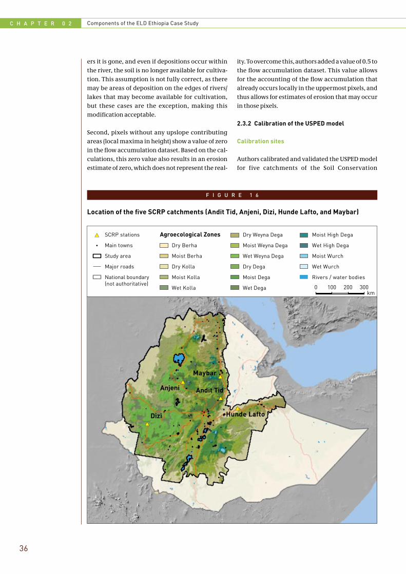
C H A P T E R 0 2 Components of the ELD Ethiopia Case Study
36
ers it is gone, and even if depositions occur within the river, the soil is no longer available for cultiva-tion. This assumption is not fully correct, as there may be areas of deposition on the edges of rivers/lakes that may become available for cultivation, but these cases are the exception, making this modification acceptable.
Second, pixels without any upslope contributing areas (local maxima in height) show a value of zero in the flow accumulation dataset. Based on the cal-culations, this zero value also results in an erosion estimate of zero, which does not represent the real-
ity. To overcome this, authors added a value of 0.5 to the flow accumulation dataset. This value allows for the accounting of the flow accumulation that already occurs locally in the uppermost pixels, and thus allows for estimates of erosion that may occur in those pixels.
2.3.2 Calibration of the USPED model
Calibration sites
Authors calibrated and validated the USPED model for five catchments of the Soil Conservation
F I G U R E 1 6
Location of the five SCRP catchments (Andit Tid, Anjeni, Dizi, Hunde Lafto, and Maybar)
!
!
! !
!
!
!
!
!!
!!
!!
! !
!
!!!
!
! !
!
!
!
#*
#*
#*
#*
#*
Anjeni
Dizi
Andit Tid
Hunde Lafto
Maybar
#*
!
0 100 200 300km
SCRP stations
Main towns
Study area
Major roads
National boundary(not authoritative)
Agroecological Zones
Dry Berha
Moist Berha
Dry Kolla
Moist Kolla
Wet Kolla
Dry Weyna Dega
Moist Weyna Dega
Wet Weyna Dega
Dry Dega
Moist Dega
Wet Dega
Moist High Dega
Wet High Dega
Moist Wurch
Wet Wurch
Rivers / water bodies
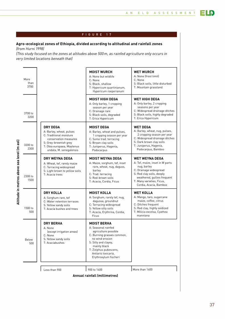
A N E L D A S S E S S M E N T
37
F I G U R E 1 7
Agro-ecological zones of Ethiopia, divided according to altitudinal and rainfall zones(from Hurni 1998)(This study focused on the zones at altitudes above 500 m, as rainfed agriculture only occurs in very limited locations beneath that)
MOIST WURCHA: None but wildlifeC: NoneS: Black, shallowT: Hypericum quartinianum, Hypericum roeperianum
WET WURCHA: None (frost limit)C: NoneS: Black soils, little disturbedT: Mountain grassland
MOIST HIGH DEGAA: Only barley, 1 cropping season per yearC: Drainage rareS: Black soils, degradedT: Erica Hypericum
WET HIGH DEGAA: Only barley, 2 cropping seasons per yearC: Widespread drainage ditchesS: Black soils, highly degradedT: Erica Hypericum
DRY DEGAA: Barley, wheat, pulsesC: Traditional moisture conservation measuresS: Grey-brownish greyT: Olea europaea, Maytenus undata, M. senegalensis
MOIST DEGAA: Barley, wheat and pulses, 1 cropping season per yearC: Some trad. terracingS: Brown clay soilsT: Juniperus, Hagenia, Podocarpus
WET DEGAA: Barley, wheat, nug, pulses, 2 cropping season per yearC: Widespread drainage ditchesS: Dark brown clay soilsT: Juniperus, Hagenia, Podocarpus, Bamboo
DRY WEYNA DEGAA: Wheat, tef, rarely maizeC: Terracing widespreadS: Light brown to yellow soilsT: Acacia trees
MOIST WEYNA DEGAA: Maize, sorghum, tef, inset rare, wheat, nug, daguss, barleyC: Trad. terracingS: Red-brown soilsT: Acacia, Cordia, Ficus
WET WEYNA DEGAA: Tef, maize, inset in W parts nug, barleyC: Drainage widespreadS: Red clay soils, deeply weathered, gullies frequentT: Many varieties, Ficus, Cordia, Acacia, Bamboo
DRY KOLLAA: Sorghum rare, tefC: Water retention terracesS: Yellow sandy soilsT: Acacia bushes and trees
MOIST KOLLAA: Sorghum, rarely tef, nug, dagussa, groundnutC: Terracing widespreadS: Yellow silty soilsT: Acacia, Erythrina, Cordia, Ficus
WET KOLLAA: Mango, taro, sugarcane maize, coffee, citrusC: Ditches frequentS: Red clay, highly oxidizedT: Milicia excelsa, Cyathea manniana
DRY BERHAA: None (except irrigation areas)C: NoneS: Yellow sandy soilsT: Acaciabushes
MOIST BERHAA: Seasonal rainfed agriculture possibleC: Burning grasses common, no wind erosionS: Silty and clayey, mainly blackT: Ziziphus pubescens, Antiaris toxicaria, Erythroxylum fischeri
More than 3700
3700 to 3200
3200 to 2300
2300 to 1500
1500 to 500
Below 500
Alt
itud
e in
met
res
abov
e se
a le
vel (
m a
sl)
Less than 900 900 to 1400 More than 1400
Annual rainfall (millimetres)
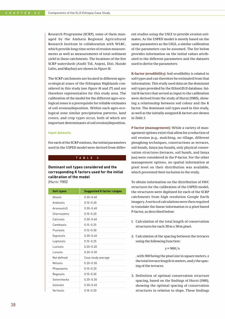
C H A P T E R 0 2 Components of the ELD Ethiopia Case Study
38
Research Programme (SCRP), some of them man-aged by the Amhara Regional Agricultural Research Institute in collaboration with WLRC, which provide long-time series of erosion measure-ments as well as measurements of total sediment yield in these catchments. The locations of the five SCRP watersheds (Andit Tid, Anjeni, Dizi, Hunde Lafto, and Maybar) are shown in Figure 16.
The SCRP catchments are located in different agro-ecological zones of the Ethiopian Highlands con-sidered in this study (see Figure 16 and 17) and are therefore representative for this study area. The calibration of the model for the different agro-eco-logical zones is a prerequisite for reliable estimates of soil erosion/deposition. Within each agro-eco-logical zone similar precipitation patterns, land covers, and crop types occur, both of which are important determinants of soil erosion/deposition.
Input datasets
For each of the SCRP stations, the initial parameters used in the USPED model were derived from differ-
T A B L E 3
Dominant soil types considered and the corresponding K factors used for the initial calibration of the model (Hurni 1985)
Soil types Suggested K factor ranges
Alisols 0.30–0.40
Andosols 0.10–0.20
ArenosolsS 0.30–0.40
Chernozems 0.10–0.20
Calcisols 0.30–0.40
Cambisols 0.15–0.25
Fluvisols 0.15–0.30
Gypsisols 0.30–0.40
Leptosols 0.15–0.25
Luvisols 0.20–0.30
Lixisols 0.20–0.30
Not defined Case study average
Nitisols 0.20–0.30
Phaeozems 0.10–0.20
Regosols 0.15–0.30
Solonchacks 0.20–0.30
Solonetz 0.30–0.40
Vertisols 0.10–0.20
ent studies using the USLE to provide erosion esti-mates. As the USPED model is mostly based on the same parameters as the USLE, a similar calibration of the parameters can be assumed. The list below provides information on the initial values attrib-uted to the different parameters and the datasets used to derive the parameters:
K-factor (erodibility): Soil erodibility is related to soil types and can therefore be estimated from that information. This study used data on the dominant soil types provided by the EthioGIS II database. Ini-tial K-factors that served as input to the calibration were derived from the study of Hurni (1985), show-ing a relationship between soil colour and the K factor. The dominant soil types used in this study, as well as the initially assigned K-factors are shown in Table 3.
P factor (management): While a variety of man-agement options exists that allow for a reduction of soil erosion (e.g., mulching, no tillage, different ploughing techniques, constructions as terraces, soil bunds, fanya juu bunds), only physical conser-vation structures (terraces, soil bunds, and fanya juu) were considered in the P-factor. For the other management options, no spatial information at pixel level on their distribution was available, which prevented their inclusion in the study.
To obtain information on the distribution of SWC structures for the calibration of the USPED model, the structures were digitized for each of the SCRP catchments from high resolution Google Earth imagery. A series of calculations were then required to translate the linear information to a pixel based P-factor, as described below:
1. Calculation of the total length of conservation structures for each 30 m x 30 m pixel.
2. Calculation of the spacing between the terraces using the following function:
y = 900 / x
, with 900 being the pixel size in square meters, x the total terrace length in meters, and y the spac-ing of the terraces.
3. Definition of optimal conservation structure spacing, based on the findings of Hurni (1981), showing the optimal spacing of conservation structures in relation to slope. These findings
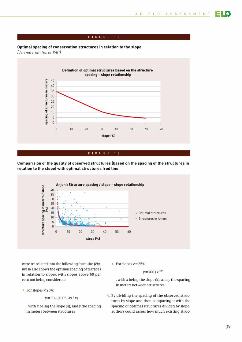
A N E L D A S S E S S M E N T
39
F I G U R E 1 8
F I G U R E 1 9
Optimal spacing of conservation structures in relation to the slope(derived from Hurni 1981)
Comparision of the quality of observed structures (based on the spacing of the structures in relation to the slope) with optimal structures (red line)
0
5
10
20
25
30
35
40
45
0 10 20 30 40 50 60 70
spac
ing
of s
truc
ture
s in
met
ers
slope (%)
Definition of optimal structures based on the structure spacing – slope relationship
05
10152025303540
0 10 20 30 40 50 60
stru
ctur
e sp
acin
g in
met
ers
/ sl
ope
(%)
slope (%)
Anjeni: Structure spacing / slope – slope relationship
Optimal structures
Structures in Anjeni
were translated into the following formulas (Fig-ure 18 also shows the optimal spacing of terraces in relation to slope), with slopes above 60 per cent not being considered:
k For slopes < 25%:
y = 30 – ( 0.65619 * x)
, with x being the slope (%), and y the spacing in meters between structures
k For slopes >= 25%:
y = 760 / x1.25
, with x being the slope (%), and y the spacing in meters between structures.
4. By dividing the spacing of the observed struc-tures by slope and then comparing it with the spacing of optimal structures divided by slope, authors could assess how much existing struc-
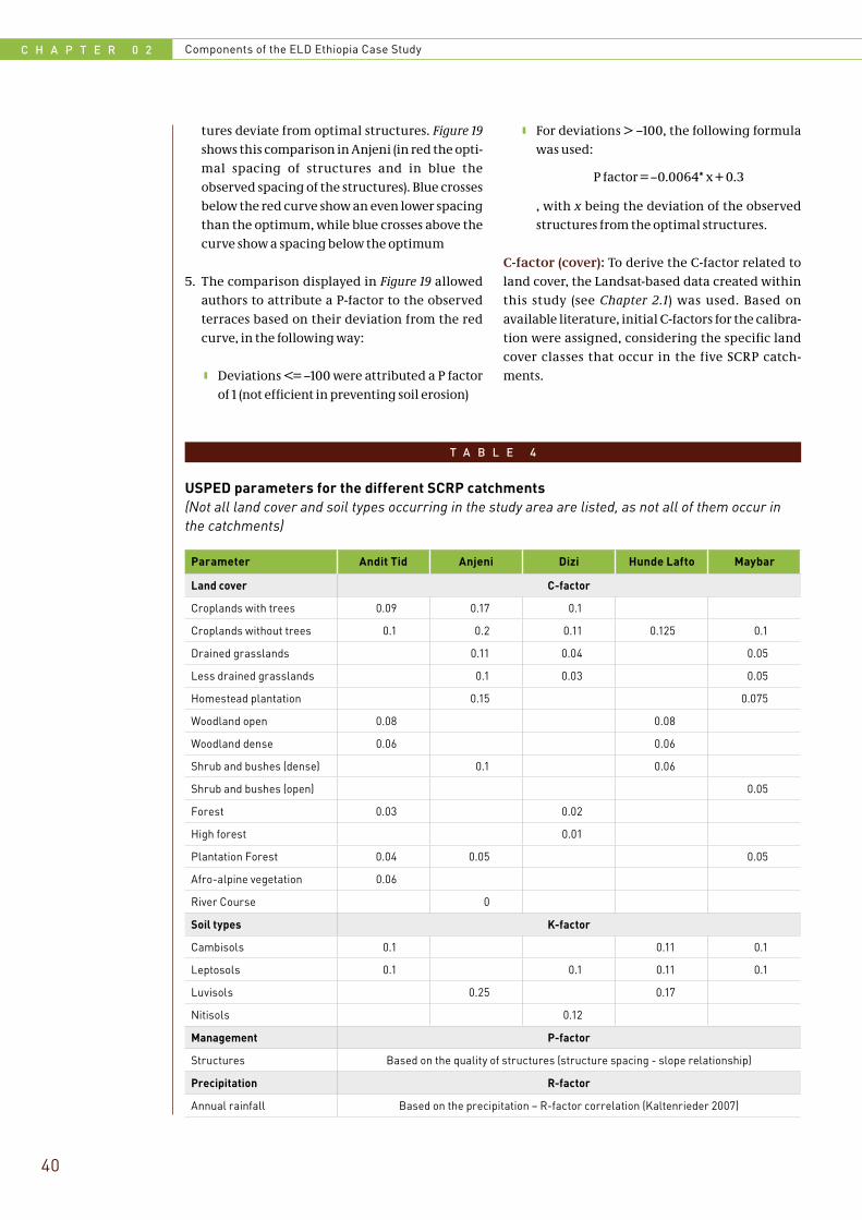
C H A P T E R 0 2 Components of the ELD Ethiopia Case Study
40
tures deviate from optimal structures. Figure 19 shows this comparison in Anjeni (in red the opti-mal spacing of structures and in blue the observed spacing of the structures). Blue crosses below the red curve show an even lower spacing than the optimum, while blue crosses above the curve show a spacing below the optimum
5. The comparison displayed in Figure 19 allowed authors to attribute a P-factor to the observed terraces based on their deviation from the red curve, in the following way:
k Deviations <= –100 were attributed a P factor of 1 (not efficient in preventing soil erosion)
k For deviations > –100, the following formula was used:
P factor = –0.0064* x + 0.3
, with x being the deviation of the observed structures from the optimal structures.
C-factor (cover): To derive the C-factor related to land cover, the Landsat-based data created within this study (see Chapter 2.1) was used. Based on available literature, initial C-factors for the calibra-tion were assigned, considering the specific land cover classes that occur in the five SCRP catch-ments.
T A B L E 4
USPED parameters for the different SCRP catchments (Not all land cover and soil types occurring in the study area are listed, as not all of them occur in the catchments)
Parameter Andit Tid Anjeni Dizi Hunde Lafto Maybar
Land cover C-factor
Croplands with trees 0.09 0.17 0.1
Croplands without trees 0.1 0.2 0.11 0.125 0.1
Drained grasslands 0.11 0.04 0.05
Less drained grasslands 0.1 0.03 0.05
Homestead plantation 0.15 0.075
Woodland open 0.08 0.08
Woodland dense 0.06 0.06
Shrub and bushes (dense) 0.1 0.06
Shrub and bushes (open) 0.05
Forest 0.03 0.02
High forest 0.01
Plantation Forest 0.04 0.05 0.05
Afro-alpine vegetation 0.06
River Course 0
Soil types K-factor
Cambisols 0.1 0.11 0.1
Leptosols 0.1 0.1 0.11 0.1
Luvisols 0.25 0.17
Nitisols 0.12
Management P-factor
Structures Based on the quality of structures (structure spacing - slope relationship)
Precipitation R-factor
Annual rainfall Based on the precipitation – R-factor correlation (Kaltenrieder 2007)
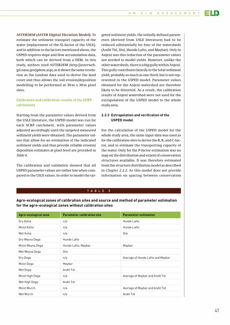
A N E L D A S S E S S M E N T
41
ASTERDEM (ASTER Digital Elevation Model): To estimate the sediment transport capacity of the water (replacement of the SL-factor of the USLE), and in addition to the factors mentioned above, the USPED requires slope and flow accumulation data, both which can be derived from a DEM. In this study, authors used ASTERDEM (http://asterweb.jpl.nasa.gov/gdem.asp), as it shows the same resolu-tion as the Landsat data used to derive the land cover and thus allows the soil erosion/deposition modelling to be performed at 30 m x 30 m pixel sizes.
Calibration and calibration results of the SCRP catchments
Starting from the parameter values derived from the USLE literature, the USPED model was run for each SCRP catchment, with parameter values adjusted accordingly until the targeted measured sediment yields were obtained. The parameter val-ues that allow for an estimation of the indicated sediment yields and thus provide reliable erosion/deposition estimates at pixel level are provided in Table 4.
The calibration and validation showed that all USPED parameter values are rather low when com-pared to the USLE values. In order to model the tar-
geted sediment yields, the initially defined param-eters (derived from USLE literature) had to be reduced substantially for four of the watersheds (Andit Tid, Dizi, Hunde Lafto, and Maybar). Only in Anjeni was this reduction of the parameter values not needed to model yields. However, unlike the other watersheds, there is a big gully within Anjeni. This gully contributes heavily to the total sediment yield, probably as much as one third, but is not rep-resented in the USPED model. Parameter values obtained for the Anjeni watershed are therefore likely to be distorted. As a result, the calibration results of Anjeni watershed were not used for the extrapolation of the USPED model to the whole study area.
2.3.3 Extrapolation and verification of the USPED model
For the calculation of the USPED model for the whole study area, the same input data was used as for the calibration sites to derive the R, K, and C-fac-tor, and to estimate the transporting capacity of the water. Only for the P-factor estimation was no map on the distribution and extent of conservation structures available. It was therefore estimated from the structure distribution model as described in Chapter 2.2.2. As this model does not provide information on spacing between conservation
T A B L E 5
Agro-ecological zones of calibration sites and source and method of parameter estimation for the agro-ecological zones without calibration sites
Agro-ecological zone Parameter calibration site Parameter estimation
Dry Kolla n/a Hunde Lafto
Moist Kolla n/a Hunde Lafto
Wet Kolla n/a Dizi
Dry Weyna Dega Hunde Lafto
Moist Weyna Dega Hunde Lafto, Maybar Maybar
Wet Weyna Dega Dizi
Dry Dega n/a Average of Hunde Lafto and Maybar
Moist Dega Maybar
Wet Dega Andit Tid
Moist High Dega n/a Average of Maybar and Andit Tid
Wet High Dega Andit Tid
Moist Wurch n/a Average of Maybar and Andit Tid
Wet Wurch n/a Andit Tid
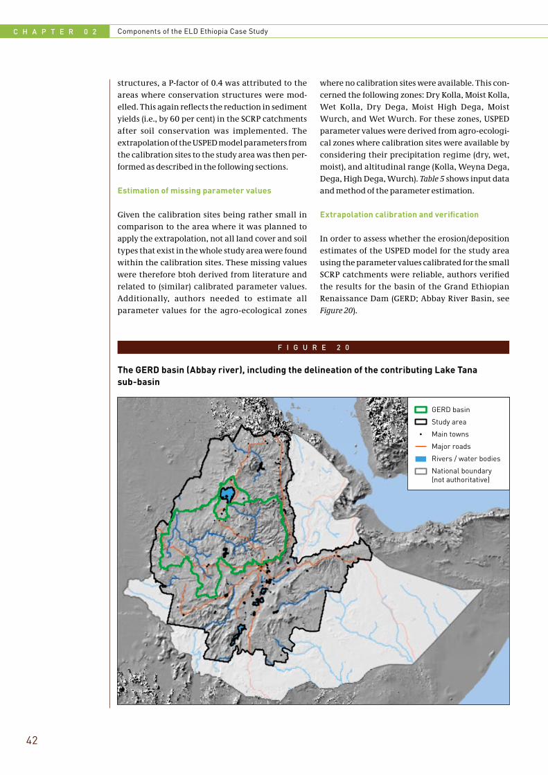
C H A P T E R 0 2 Components of the ELD Ethiopia Case Study
42
structures, a P-factor of 0.4 was attributed to the areas where conservation structures were mod-elled. This again reflects the reduction in sediment yields (i.e., by 60 per cent) in the SCRP catchments after soil conservation was implemented. The extrapolation of the USPED model parameters from the calibration sites to the study area was then per-formed as described in the following sections.
Estimation of missing parameter values
Given the calibration sites being rather small in comparison to the area where it was planned to apply the extrapolation, not all land cover and soil types that exist in the whole study area were found within the calibration sites. These missing values were therefore btoh derived from literature and related to (similar) calibrated parameter values. Additionally, authors needed to estimate all parameter values for the agro-ecological zones
where no calibration sites were available. This con-cerned the following zones: Dry Kolla, Moist Kolla, Wet Kolla, Dry Dega, Moist High Dega, Moist Wurch, and Wet Wurch. For these zones, USPED parameter values were derived from agro-ecologi-cal zones where calibration sites were available by considering their precipitation regime (dry, wet, moist), and altitudinal range (Kolla, Weyna Dega, Dega, High Dega, Wurch). Table 5 shows input data and method of the parameter estimation.
Extrapolation calibration and verification
In order to assess whether the erosion/deposition estimates of the USPED model for the study area using the parameter values calibrated for the small SCRP catchments were reliable, authors verified the results for the basin of the Grand Ethiopian Renaissance Dam (GERD; Abbay River Basin, see Figure 20).
F I G U R E 2 0
The GERD basin (Abbay river), including the delineation of the contributing Lake Tana sub-basin
!
GERD basin
Study area
Main towns
Major roads
Rivers / water bodies
National boundary(not authoritative)
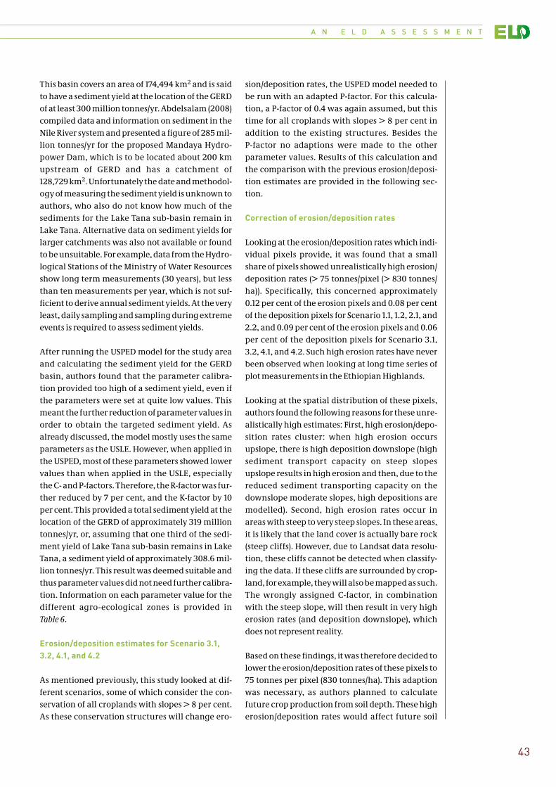
A N E L D A S S E S S M E N T
43
This basin covers an area of 174,494 km2 and is said to have a sediment yield at the location of the GERD of at least 300 million tonnes/yr. Abdelsalam (2008) compiled data and information on sediment in the Nile River system and presented a figure of 285 mil-lion tonnes/yr for the proposed Mandaya Hydro-power Dam, which is to be located about 200 km upstream of GERD and has a catchment of 128,729 km2. Unfortunately the date and methodol-ogy of measuring the sediment yield is unknown to authors, who also do not know how much of the sediments for the Lake Tana sub-basin remain in Lake Tana. Alternative data on sediment yields for larger catchments was also not available or found to be unsuitable. For example, data from the Hydro-logical Stations of the Ministry of Water Resources show long term measurements (30 years), but less than ten measurements per year, which is not suf-ficient to derive annual sediment yields. At the very least, daily sampling and sampling during extreme events is required to assess sediment yields.
After running the USPED model for the study area and calculating the sediment yield for the GERD basin, authors found that the parameter calibra-tion provided too high of a sediment yield, even if the parameters were set at quite low values. This meant the further reduction of parameter values in order to obtain the targeted sediment yield. As already discussed, the model mostly uses the same parameters as the USLE. However, when applied in the USPED, most of these parameters showed lower values than when applied in the USLE, especially the C- and P-factors. Therefore, the R-factor was fur-ther reduced by 7 per cent, and the K-factor by 10 per cent. This provided a total sediment yield at the location of the GERD of approximately 319 million tonnes/yr, or, assuming that one third of the sedi-ment yield of Lake Tana sub-basin remains in Lake Tana, a sediment yield of approximately 308.6 mil-lion tonnes/yr. This result was deemed suitable and thus parameter values did not need further calibra-tion. Information on each parameter value for the different agro-ecological zones is provided in Table 6.
Erosion/deposition estimates for Scenario 3.1, 3.2, 4.1, and 4.2
As mentioned previously, this study looked at dif-ferent scenarios, some of which consider the con-servation of all croplands with slopes > 8 per cent. As these conservation structures will change ero-
sion/deposition rates, the USPED model needed to be run with an adapted P-factor. For this calcula-tion, a P-factor of 0.4 was again assumed, but this time for all croplands with slopes > 8 per cent in addition to the existing structures. Besides the P-factor no adaptions were made to the other parameter values. Results of this calculation and the comparison with the previous erosion/deposi-tion estimates are provided in the following sec-tion.
Correction of erosion/deposition rates
Looking at the erosion/deposition rates which indi-vidual pixels provide, it was found that a small share of pixels showed unrealistically high erosion/deposition rates (> 75 tonnes/pixel (> 830 tonnes/ha)). Specifically, this concerned approximately 0.12 per cent of the erosion pixels and 0.08 per cent of the deposition pixels for Scenario 1.1, 1.2, 2.1, and 2.2, and 0.09 per cent of the erosion pixels and 0.06 per cent of the deposition pixels for Scenario 3.1, 3.2, 4.1, and 4.2. Such high erosion rates have never been observed when looking at long time series of plot measurements in the Ethiopian Highlands.
Looking at the spatial distribution of these pixels, authors found the following reasons for these unre-alistically high estimates: First, high erosion/depo-sition rates cluster: when high erosion occurs upslope, there is high deposition downslope (high sediment transport capacity on steep slopes upslope results in high erosion and then, due to the reduced sediment transporting capacity on the downslope moderate slopes, high depositions are modelled). Second, high erosion rates occur in areas with steep to very steep slopes. In these areas, it is likely that the land cover is actually bare rock (steep cliffs). However, due to Landsat data resolu-tion, these cliffs cannot be detected when classify-ing the data. If these cliffs are surrounded by crop-land, for example, they will also be mapped as such. The wrongly assigned C-factor, in combination with the steep slope, will then result in very high erosion rates (and deposition downslope), which does not represent reality.
Based on these findings, it was therefore decided to lower the erosion/deposition rates of these pixels to 75 tonnes per pixel (830 tonnes/ha). This adaption was necessary, as authors planned to calculate future crop production from soil depth. These high erosion/deposition rates would affect future soil
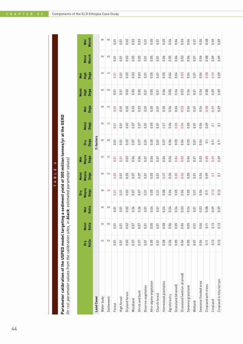
C H A P T E R 0 2 Components of the ELD Ethiopia Case Study
44
TA
BL
E
6
Par
amet
er c
alib
rati
on o
f the
USP
ED
mod
el ta
rget
ing
a se
dim
ent y
ield
of 3
00 m
illi
on to
nnes
/yr
at th
e G
ER
D(In
red
: par
amet
er v
alue
s fr
om th
e ca
libra
tion
site
s, in
bla
ck: e
stim
ated
par
amet
er v
alue
s)
Dry
K
olla
Moi
st
Kol
laW
et
Kol
la
Dry
W
eyna
D
ega
Moi
st
Wey
na
Deg
a
Wet
W
eyna
D
ega
Dry
D
ega
Moi
st
Deg
aW
et
Deg
a
Moi
st
Hig
h D
ega
Wet
H
igh
Deg
aM
oist
W
urch
Wet
W
urch
Land
Cov
erC
-fac
tors
Wat
er b
ody
00
00
00
00
00
00
0
Sett
lem
ent
00
00
00
00
00
00
0
Fore
st0.
010.
010.
010.
010.
010.
010.
010.
010.
010.
010.
010.
010.
01
Hig
h fo
rest
0.01
0.01
0.01
0.01
0.01
0.01
0.01
0.01
0.01
0.01
0.01
0.01
0.01
Dry
land
fore
st0.
020.
020.
020.
020.
020.
020.
020.
020.
020.
020.
020.
020.
02
Woo
dlan
d0.
070.
070.
060.
070.
070.
060.
070.
070.
030.
050.
030.
050.
03
Shru
b an
d bu
sh0.
070.
070.
060.
070.
070.
060.
070.
070.
030.
050.
030.
050.
03
Riv
erin
e ve
geta
tion
0.01
0.01
0.01
0.01
0.01
0.01
0.01
0.01
0.01
0.01
0.01
0.01
0.01
Afr
o-al
pine
veg
etat
ion
0.05
0.05
0.04
0.05
0.05
0.04
0.05
0.05
0.05
0.05
0.05
0.05
0.05
Chu
rch
fore
st0.
010.
010.
010.
010.
010.
010.
010.
010.
010.
010.
010.
010.
01
Hom
este
ad p
lant
atio
n0.
080.
080.
040.
080.
070.
040.
070.
070.
050.
060.
050.
060.
05
Agro
fore
stry
0.06
0.06
0.04
0.06
0.06
0.04
0.06
0.06
0.04
0.05
0.04
0.05
0.04
Gra
ssla
nd (d
rain
ed)
0.05
0.05
0.04
0.05
0.05
0.04
0.05
0.05
0.04
0.04
0.04
0.04
0.04
Gra
ssla
nd (w
et/u
n-dr
aine
d)0.
040.
040.
030.
040.
040.
030.
040.
040.
030.
030.
030.
030.
03
Sava
nna
gras
slan
d0.
050.
050.
040.
050.
050.
040.
050.
050.
040.
040.
040.
040.
04
Wet
land
0.01
0.01
0.01
0.01
0.01
0.01
0.01
0.01
0.01
0.01
0.01
0.01
0.01
Seas
onal
floo
ded
area
0.04
0.04
0.03
0.04
0.04
0.03
0.04
0.04
0.04
0.04
0.04
0.04
0.04
Cro
plan
d w
ith tr
ees
0.11
0.11
0.08
0.11
0.09
0.08
0.1
0.09
0.08
0.08
0.08
0.08
0.08
Cro
plan
d0.
130.
130.
090.
130.
10.
090.
110.
10.
090.
090.
090.
090.
09
Cro
plan
d in
hill
y te
rrai
n0.
130.
130.
090.
130.
10.
090.
110.
10.
090.
090.
090.
090.
09
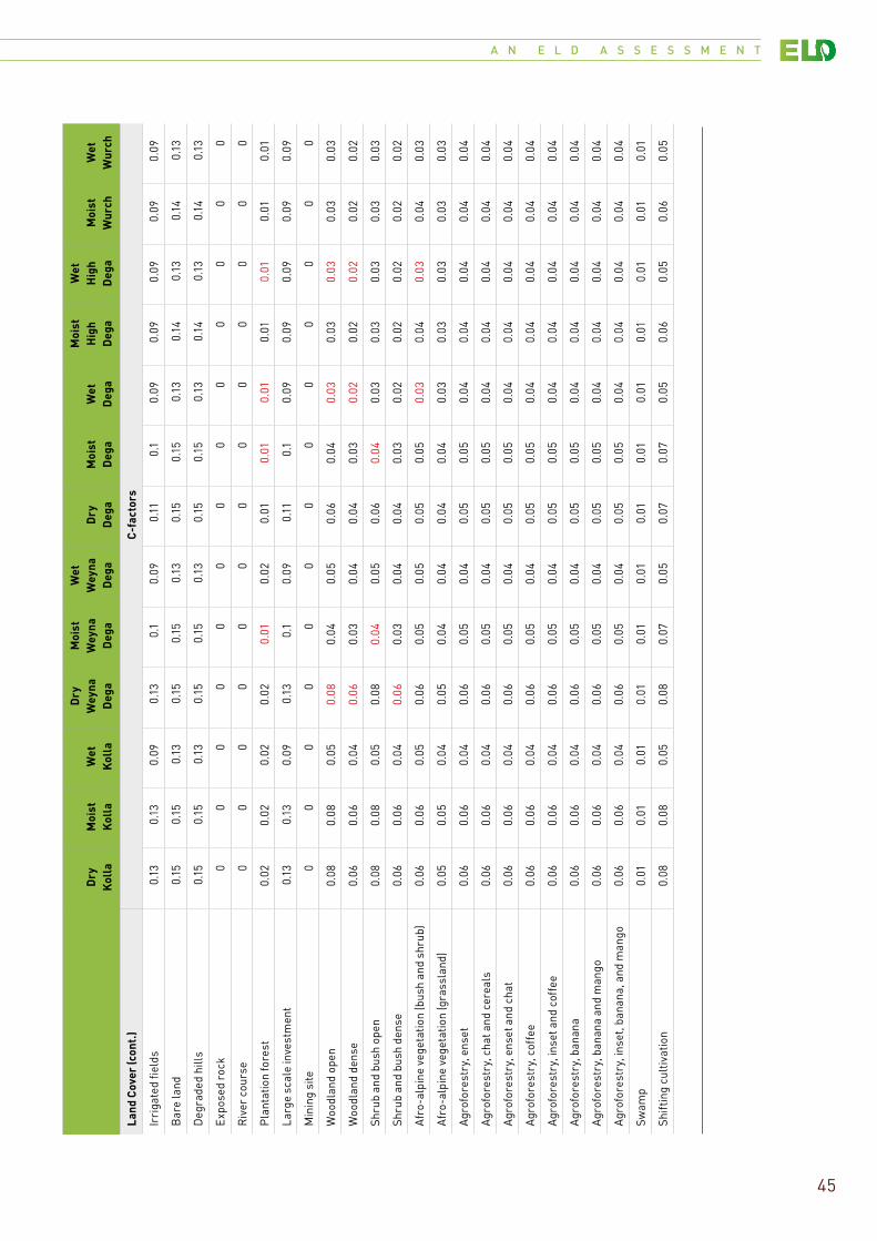
A N E L D A S S E S S M E N T
45
Dry
K
olla
Moi
st
Kol
laW
et
Kol
la
Dry
W
eyna
D
ega
Moi
st
Wey
na
Deg
a
Wet
W
eyna
D
ega
Dry
D
ega
Moi
st
Deg
aW
et
Deg
a
Moi
st
Hig
h D
ega
Wet
H
igh
Deg
aM
oist
W
urch
Wet
W
urch
Land
Cov
er (c
ont.
)C
-fac
tors
Irri
gate
d fie
lds
0.13
0.13
0.09
0.13
0.1
0.09
0.11
0.1
0.09
0.09
0.09
0.09
0.09
Bar
e la
nd0.
150.
150.
130.
150.
150.
130.
150.
150.
130.
140.
130.
140.
13
Deg
rade
d hi
lls
0.15
0.15
0.13
0.15
0.15
0.13
0.15
0.15
0.13
0.14
0.13
0.14
0.13
Exp
osed
roc
k0
00
00
00
00
00
00
Riv
er c
ours
e0
00
00
00
00
00
00
Pla
ntat
ion
fore
st0.
020.
020.
020.
020.
010.
020.
010.
010.
010.
010.
010.
010.
01
Larg
e sc
ale
inve
stm
ent
0.13
0.13
0.09
0.13
0.1
0.09
0.11
0.1
0.09
0.09
0.09
0.09
0.09
Min
ing
site
00
00
00
00
00
00
0
Woo
dlan
d op
en0.
080.
080.
050.
080.
040.
050.
060.
040.
030.
030.
030.
030.
03
Woo
dlan
d de
nse
0.06
0.06
0.04
0.06
0.03
0.04
0.04
0.03
0.02
0.02
0.02
0.02
0.02
Shru
b an
d bu
sh o
pen
0.08
0.08
0.05
0.08
0.04
0.05
0.06
0.04
0.03
0.03
0.03
0.03
0.03
Shru
b an
d bu
sh d
ense
0.06
0.06
0.04
0.06
0.03
0.04
0.04
0.03
0.02
0.02
0.02
0.02
0.02
Afr
o-al
pine
veg
etat
ion
(bus
h an
d sh
rub)
0.06
0.06
0.05
0.06
0.05
0.05
0.05
0.05
0.03
0.04
0.03
0.04
0.03
Afr
o-al
pine
veg
etat
ion
(gra
ssla
nd)
0.05
0.05
0.04
0.05
0.04
0.04
0.04
0.04
0.03
0.03
0.03
0.03
0.03
Agro
fore
stry
, ens
et0.
060.
060.
040.
060.
050.
040.
050.
050.
040.
040.
040.
040.
04
Agro
fore
stry
, cha
t and
cer
eals
0.06
0.06
0.04
0.06
0.05
0.04
0.05
0.05
0.04
0.04
0.04
0.04
0.04
Agro
fore
stry
, ens
et a
nd c
hat
0.06
0.06
0.04
0.06
0.05
0.04
0.05
0.05
0.04
0.04
0.04
0.04
0.04
Agro
fore
stry
, cof
fee
0.06
0.06
0.04
0.06
0.05
0.04
0.05
0.05
0.04
0.04
0.04
0.04
0.04
Agro
fore
stry
, ins
et a
nd c
offe
e0.
060.
060.
040.
060.
050.
040.
050.
050.
040.
040.
040.
040.
04
Agro
fore
stry
, ban
ana
0.06
0.06
0.04
0.06
0.05
0.04
0.05
0.05
0.04
0.04
0.04
0.04
0.04
Agro
fore
stry
, ban
ana
and
man
go0.
060.
060.
040.
060.
050.
040.
050.
050.
040.
040.
040.
040.
04
Agro
fore
stry
, ins
et, b
anan
a, a
nd m
ango
0.06
0.06
0.04
0.06
0.05
0.04
0.05
0.05
0.04
0.04
0.04
0.04
0.04
Swam
p0.
010.
010.
010.
010.
010.
010.
010.
010.
010.
010.
010.
010.
01
Shift
ing
cult
ivat
ion
0.08
0.08
0.05
0.08
0.07
0.05
0.07
0.07
0.05
0.06
0.05
0.06
0.05
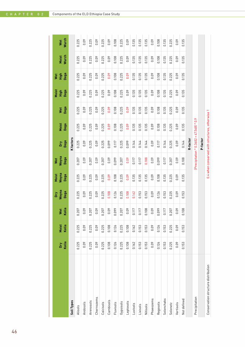
C H A P T E R 0 2 Components of the ELD Ethiopia Case Study
46
Dry
K
olla
Moi
st
Kol
laW
et
Kol
la
Dry
W
eyna
D
ega
Moi
st
Wey
na
Deg
a
Wet
W
eyna
D
ega
Dry
D
ega
Moi
st
Deg
aW
et
Deg
a
Moi
st
Hig
h D
ega
Wet
H
igh
Deg
aM
oist
W
urch
Wet
W
urch
Soil
Type
sK
fact
ors
Alis
ols
0.22
50.
225
0.20
70.
225
0.22
50.
207
0.22
50.
225
0.22
50.
225
0.22
50.
225
0.22
5
And
osol
s0.
090.
090.
090.
090.
090.
090.
090.
090.
090.
090.
090.
090.
09
Are
noso
ls0.
225
0.22
50.
207
0.22
50.
225
0.20
70.
225
0.22
50.
225
0.22
50.
225
0.22
50.
225
Che
rnoz
ems
0.09
0.09
0.09
0.09
0.09
0.09
0.09
0.09
0.09
0.09
0.09
0.09
0.09
Cal
ciso
ls0.
225
0.22
50.
207
0.22
50.
225
0.20
70.
225
0.22
50.
225
0.22
50.
225
0.22
50.
225
Cam
biso
ls0.
108
0.10
80.
090.
108
0.09
0.09
0.09
90.
090.
090.
090.
090.
090.
09
Fluv
isol
s0.
126
0.12
60.
099
0.12
60.
108
0.09
90.
117
0.10
80.
108
0.10
80.
108
0.10
80.
108
Gyp
siso
ls0.
225
0.22
50.
207
0.22
50.
225
0.20
70.
225
0.22
50.
225
0.22
50.
225
0.22
50.
225
Lept
osol
s0.
108
0.10
80.
090.
108
0.09
0.09
0.09
90.
090.
090.
090.
090.
090.
09
Luvi
sols
0.16
20.
162
0.11
70.
162
0.13
50.
117
0.14
40.
135
0.13
50.
135
0.13
50.
135
0.13
5
Lixi
sols
0.15
30.
153
0.11
70.
153
0.13
50.
117
0.14
40.
135
0.13
50.
135
0.13
50.
135
0.13
5
Niti
sols
0.15
30.
153
0.10
80.
153
0.13
50.
108
0.14
40.
135
0.13
50.
135
0.13
50.
135
0.13
5
Pha
eoze
ms
0.09
0.09
0.09
0.09
0.09
0.09
0.09
0.09
0.09
0.09
0.09
0.09
0.09
Reg
osol
s0.
126
0.12
60.
099
0.12
60.
108
0.09
90.
117
0.10
80.
108
0.10
80.
108
0.10
80.
108
Solo
ncha
ks0.
153
0.15
30.
117
0.15
30.
135
0.11
70.
144
0.13
50.
135
0.13
50.
135
0.13
50.
135
Solo
netz
0.22
50.
225
0.20
70.
225
0.22
50.
207
0.22
50.
225
0.22
50.
225
0.22
50.
225
0.22
5
Vert
isol
s0.
090.
090.
090.
090.
090.
090.
090.
090.
090.
090.
090.
090.
09
Not
defi
ned
0.15
30.
153
0.10
80.
153
0.13
50.
108
0.14
40.
135
0.13
50.
135
0.13
50.
135
0.13
5
R-f
acto
r
Pre
cipi
tatio
n(P
reci
pita
tion
* 0.
3602
+ 4
7.56
8) *
0.9
P-fa
ctor
Con
serv
atio
n st
ruct
ure
dist
ribu
tion
0.4
whe
n co
nser
ved
with
str
uctu
res,
oth
erw
ise
1
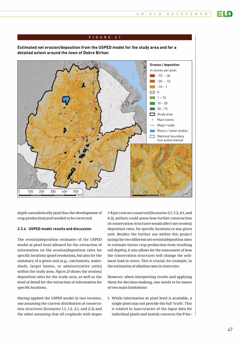
A N E L D A S S E S S M E N T
47
depth unrealistically (and thus the development of crop production) and needed to be corrected.
2.3.4 USPED model results and discussion
The erosion/deposition estimates of the USPED model at pixel level allowed for the extraction of information on the erosion/deposition rates for specific locations (pixel resolution), but also for the summary of a given unit (e.g., catchments, water-sheds, larger basins, or administrative units) within the study area. Figure 21 shows the erosion/deposition rates for the study area, as well as the level of detail for the extraction of information for specific locations.
Having applied the USPED model in two versions, one assuming the current distribution of conserva-tion structures (Scenarios 1.1, 1.2, 2.1, and 2.2) and the other assuming that all croplands with slopes
> 8 per cent are conserved (Scenarios 3.1, 3.2, 4.1, and 4.2), authors could assess how further construction of conservation structures would affect net erosion/deposition rates, for specific locations or any given unit. Besides the further use within this project (using the two different net erosion/deposition rates to estimate future crop production from resulting soil depths), it also allows for the assessment of how the conservation structures will change the sedi-ment load in rivers. This is crucial, for example, in the estimation of siltation rates in reservoirs.
However, when interpreting results and applying them for decision-making, one needs to be aware of two main limitations:
1. While information at pixel level is available, a single pixel may not provide the full ‘truth’. This is related to inaccuracies of the input data for individual pixels and mainly concerns the P-fac-
F I G U R E 2 1
Estimated net erosion/deposition from the USPED model for the study area and for a detailed extent around the town of Debre Birhan
Debre Birhan!
0 2.5 5km
0 100 200 300 400 500km
!
-75 – -30
-30 – -10
-10 – 1
0
1 – 10
10 – 30
30 – 75
Study area
Main towns
Major roads
Rivers / water bodies
National boundary(not authoritative)
Erosion / deposition
in tonnes per pixel
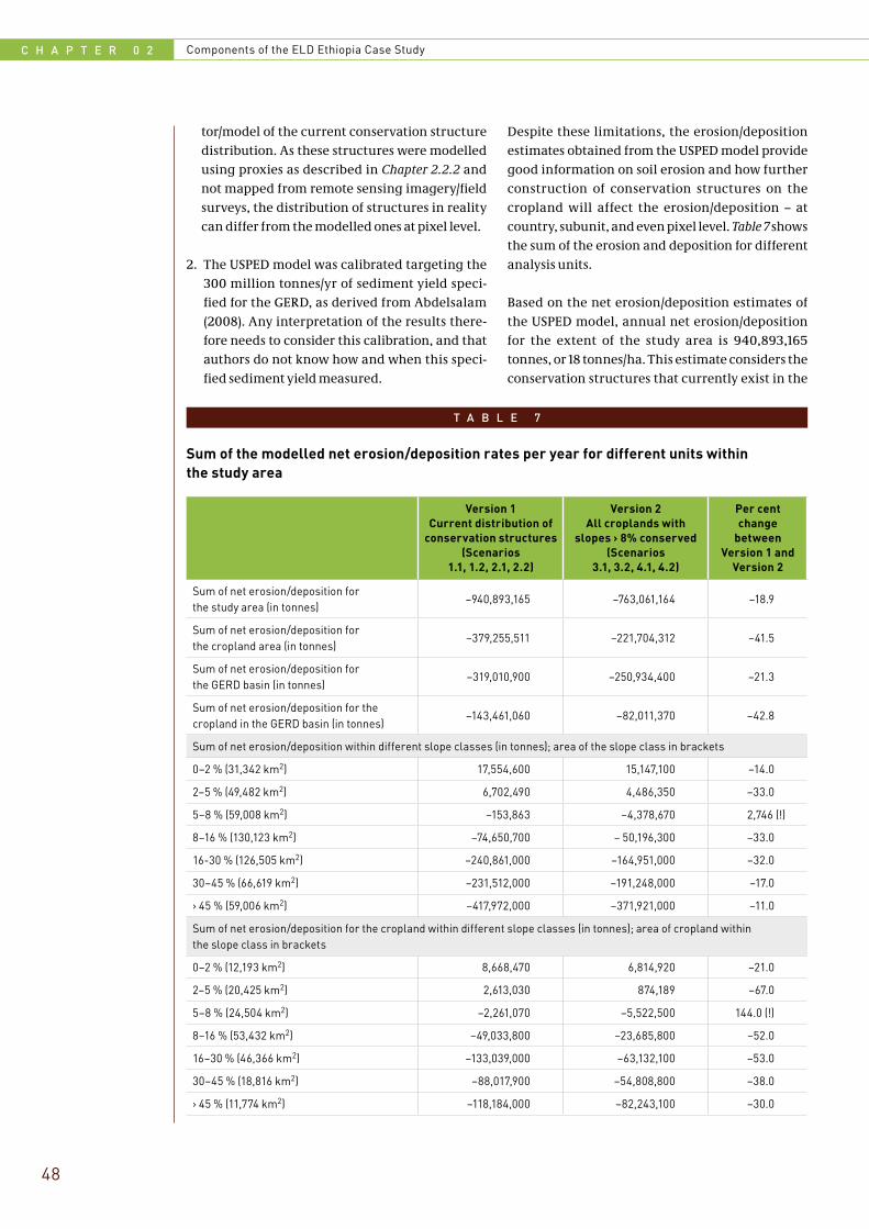
C H A P T E R 0 2 Components of the ELD Ethiopia Case Study
48
tor/model of the current conservation structure distribution. As these structures were modelled using proxies as described in Chapter 2.2.2 and not mapped from remote sensing imagery/field surveys, the distribution of structures in reality can differ from the modelled ones at pixel level.
2. The USPED model was calibrated targeting the 300 million tonnes/yr of sediment yield speci-fied for the GERD, as derived from Abdelsalam (2008). Any interpretation of the results there-fore needs to consider this calibration, and that authors do not know how and when this speci-fied sediment yield measured.
Despite these limitations, the erosion/deposition estimates obtained from the USPED model provide good information on soil erosion and how further construction of conservation structures on the cropland will affect the erosion/deposition – at country, subunit, and even pixel level. Table 7 shows the sum of the erosion and deposition for different analysis units.
Based on the net erosion/deposition estimates of the USPED model, annual net erosion/deposition for the extent of the study area is 940,893,165 tonnes, or 18 tonnes/ha. This estimate considers the conservation structures that currently exist in the
T A B L E 7
Sum of the modelled net erosion/deposition rates per year for different units within the study area
Version 1 Current distribution of
conservation structures (Scenarios
1.1, 1.2, 2.1, 2.2)
Version 2 All croplands with
slopes › 8% conserved (Scenarios
3.1, 3.2, 4.1, 4.2)
Per cent change
between Version 1 and
Version 2
Sum of net erosion/deposition for the study area (in tonnes)
–940,893,165 –763,061,164 –18.9
Sum of net erosion/deposition for the cropland area (in tonnes)
–379,255,511 –221,704,312 –41.5
Sum of net erosion/deposition for the GERD basin (in tonnes)
–319,010,900 –250,934,400 –21.3
Sum of net erosion/deposition for the cropland in the GERD basin (in tonnes)
–143,461,060 –82,011,370 –42.8
Sum of net erosion/deposition within different slope classes (in tonnes); area of the slope class in brackets
0–2 % (31,342 km2) 17,554,600 15,147,100 –14.0
2–5 % (49,482 km2) 6,702,490 4,486,350 –33.0
5–8 % (59,008 km2) –153,863 –4,378,670 2,746 (!)
8–16 % (130,123 km2) –74,650,700 – 50,196,300 –33.0
16-30 % (126,505 km2) –240,861,000 –164,951,000 –32.0
30–45 % (66,619 km2) –231,512,000 –191,248,000 –17.0
› 45 % (59,006 km2) –417,972,000 –371,921,000 –11.0
Sum of net erosion/deposition for the cropland within different slope classes (in tonnes); area of cropland within the slope class in brackets
0–2 % (12,193 km2) 8,668,470 6,814,920 –21.0
2–5 % (20,425 km2) 2,613,030 874,189 –67.0
5–8 % (24,504 km2) –2,261,070 –5,522,500 144.0 (!)
8–16 % (53,432 km2) –49,033,800 –23,685,800 –52.0
16–30 % (46,366 km2) –133,039,000 –63,132,100 –53.0
30–45 % (18,816 km2) –88,017,900 –54,808,800 –38.0
› 45 % (11,774 km2) –118,184,000 –82,243,100 –30.0

A N E L D A S S E S S M E N T
49
study area (mostly established on croplands, and in parts of Tigray and Wello also on degraded hills, grassland, shrub, and bushland). When looking at only the cropland area considered in the USPED model, 3,354,393 ha out of 18,751,262 ha of crop-land are currently conserved (17.9 per cent). How-ever, 76.5 per cent of the croplands considered in the study area show slopes > 8 per cent. In order to also conserve these areas, conservation structures need to be built on an additional 58.6 per cent of the cropland (122,077,141 ha). This was considered in Version 2 of the erosion/deposition model, and assumed that all croplands with slopes > 8 per cent are conserved. In this case, annual net erosion/dep-osition could be reduced to 763,061,164 tonnes, or 14.6 tonnes/ha (including the existing structures in parts of Tigray and Wello outside of the cropland). This would mean a reduction of the annual net soil erosion by 4 tonnes/ha.
Only looking at net erosion/deposition on crop-land, currently an annual net erosion/deposition of –379,255,511 tonnes (–20.2 tonnes/ha) is observed, which could be reduced to –221,704,312 tonnes (–11.8 tonnes/ha). This reduction of the erosion by
41.5 per cent (8.4 tonnes/ha) would have a positive effect, as every year 0.84 mm of topsoil would remain on the fields instead of being washed away.The situation in the GERD basin looks similar to the whole study area: the additional structures on cropland with slopes > 8 per cent could reduce overall net erosion from all land cover classes by 21.3 per cent, and even by 42.8 per cent when only considering cropland. In absolute values this would mean a reduction from –319,010,900 tonnes/yr to –250,934,400 tonnes/yr. However, one needs to consider that the USPED model was calibrated to approximately deliver the 300 million tonnes of sediment yield estimated for the GERD even though it is not actually known how and when this figure was measured/ estimated (Abdelsalam 2008).
When looking at the modelled erosion/deposition rates for the different slope classes, a clear pattern can be observed (see Figure 22): slopes of 0–5 per cent show deposition, while slopes > 5 per cent show erosion, whether being conserved with struc-tures or not. When comparing the two versions (current conservation, and conservation of crop-lands with slopes > 8 per cent), an interesting effect
F I G U R E 2 2
Annual net erosion/deposition for different units (complete study area and cropland only) and the two models (current distribution of conservation structures and all croplands with slopes › 8 per cent conserved)(To make the comparably small net erosion/deposition values of the slope classes 2–5 per cent and 5–8 per cent visible, erosion rates of slopes › 16 per cent are not displayed)
–10
–8
–6
–4
–2
0
2
4
6
8
0–2% 2–5% 5–8% 8–16%
Ann
ual n
et e
rosi
on /
dep
osit
ion
(t/h
a)
Slope classes
Annual net erosion/deposition of the two models
Current distribution ofconservation structures(study area)
All croplands with slopes ›8%conserved (study area)
Current distribution ofconservation structures(cropland only)
All croplands with slopes ›8%conserved (cropland only)
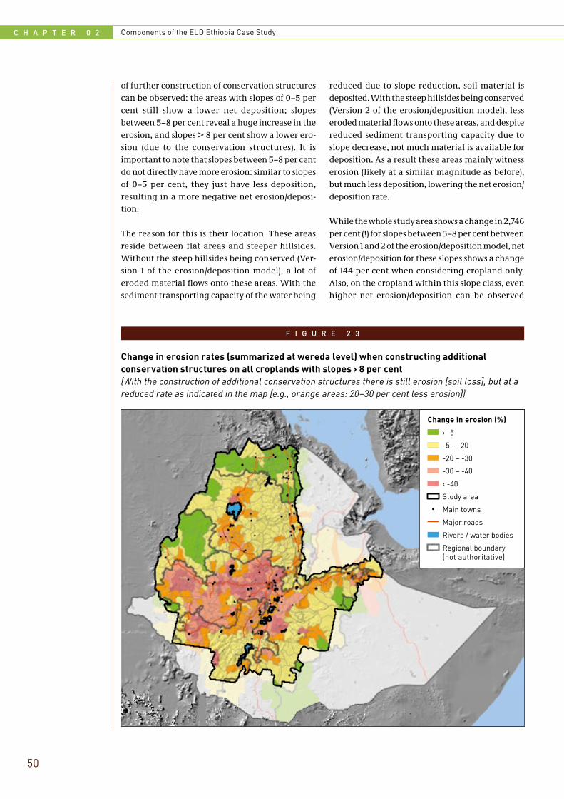
C H A P T E R 0 2 Components of the ELD Ethiopia Case Study
50
of further construction of conservation structures can be observed: the areas with slopes of 0–5 per cent still show a lower net deposition; slopes between 5–8 per cent reveal a huge increase in the erosion, and slopes > 8 per cent show a lower ero-sion (due to the conservation structures). It is important to note that slopes between 5–8 per cent do not directly have more erosion: similar to slopes of 0–5 per cent, they just have less deposition, resulting in a more negative net erosion/deposi-tion.
The reason for this is their location. These areas reside between flat areas and steeper hillsides. Without the steep hillsides being conserved (Ver-sion 1 of the erosion/deposition model), a lot of eroded material flows onto these areas. With the sediment transporting capacity of the water being
reduced due to slope reduction, soil material is deposited. With the steep hillsides being conserved (Version 2 of the erosion/deposition model), less eroded material flows onto these areas, and despite reduced sediment transporting capacity due to slope decrease, not much material is available for deposition. As a result these areas mainly witness erosion (likely at a similar magnitude as before), but much less deposition, lowering the net erosion/deposition rate.
While the whole study area shows a change in 2,746 per cent (!) for slopes between 5–8 per cent between Version 1 and 2 of the erosion/deposition model, net erosion/deposition for these slopes shows a change of 144 per cent when considering cropland only. Also, on the cropland within this slope class, even higher net erosion/deposition can be observed
F I G U R E 2 3
Change in erosion rates (summarized at wereda level) when constructing additional conservation structures on all croplands with slopes › 8 per cent(With the construction of additional conservation structures there is still erosion [soil loss], but at a reduced rate as indicated in the map [e.g., orange areas: 20–30 per cent less erosion])
!
Change in erosion (%)
› -5
-5 – -20
-20 – -30
-30 – -40
‹ -40
Study area
Main towns
Major roads
Rivers / water bodies
Regional boundary(not authoritative)

A N E L D A S S E S S M E N T
51
than in the whole study area. This big difference in the erosion/deposition rates relates to land cover: generally, cropland shows more erosion (and less deposition) than, for example, grasslands, bush-lands, or forests. Without upslope conservation (Version 1), there is thus not so much deposition on cropland when compared to other land covers, which show a lot of deposition. With upslope con-servation (Version 2), the situation for cropland does not change that much, but with less sediment being transported onto the other land covers, there is less deposition, which results in a much lower net erosion/deposition.
The construction of conservation structures on slopes > 8 per cent within cropland has thus a two-sided effect. On one hand, overall net erosion for the study area is reduced and erosion rates on the con-
served cropland are heavily reduced. On the other hand, erosion rates on the gentle sloping land (5–8 percent) increase, especially on the cropland, as there is less deposition in these areas. In the long run it seems therefore beneficial to also conserve the gently sloping croplands below 8 per cent gradients.
To assess which weredas could show the biggest reduction in soil erosion by building conservation structures on slopes > 8 per cent where no conser-vation structures exist, authors calculated the per cent change in erosion rates between Version 1 and 2 of the erosion/deposition estimates. Figure 23 shows the distribution of change in erosion rates.
In relation to the findings presented in Table 7, Fig-ure 23 clearly shows that despite the increase in ero-sion rates on gentle slopes when constructing con-
F I G U R E 2 4
Net erosion/deposition in tonnes per hectare (summarized per wereda) considering the current distribution of conservation structures(Note that all area averages are negative [net erosion])
!
‹ -30
-30 – -20
-20 – -10
-10 – -5
› -5
Study area
Main towns
Major roads
Rivers / water bodies
Regional boundary(not authoritative)
Erosion in t / ha
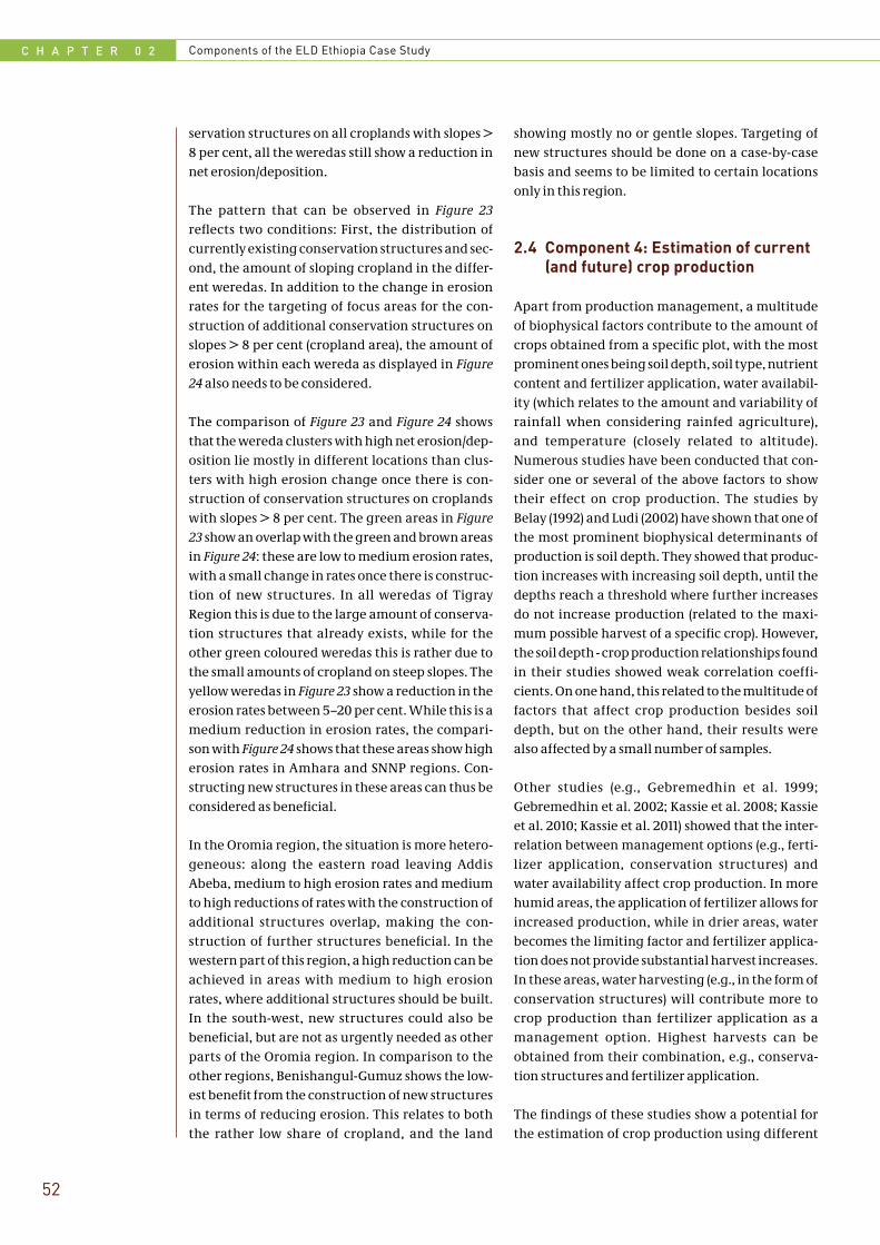
C H A P T E R 0 2 Components of the ELD Ethiopia Case Study
52
servation structures on all croplands with slopes > 8 per cent, all the weredas still show a reduction in net erosion/deposition.
The pattern that can be observed in Figure 23 reflects two conditions: First, the distribution of currently existing conservation structures and sec-ond, the amount of sloping cropland in the differ-ent weredas. In addition to the change in erosion rates for the targeting of focus areas for the con-struction of additional conservation structures on slopes > 8 per cent (cropland area), the amount of erosion within each wereda as displayed in Figure 24 also needs to be considered.
The comparison of Figure 23 and Figure 24 shows that the wereda clusters with high net erosion/dep-osition lie mostly in different locations than clus-ters with high erosion change once there is con-struction of conservation structures on croplands with slopes > 8 per cent. The green areas in Figure 23 show an overlap with the green and brown areas in Figure 24: these are low to medium erosion rates, with a small change in rates once there is construc-tion of new structures. In all weredas of Tigray Region this is due to the large amount of conserva-tion structures that already exists, while for the other green coloured weredas this is rather due to the small amounts of cropland on steep slopes. The yellow weredas in Figure 23 show a reduction in the erosion rates between 5–20 per cent. While this is a medium reduction in erosion rates, the compari-son with Figure 24 shows that these areas show high erosion rates in Amhara and SNNP regions. Con-structing new structures in these areas can thus be considered as beneficial.
In the Oromia region, the situation is more hetero-geneous: along the eastern road leaving Addis Abeba, medium to high erosion rates and medium to high reductions of rates with the construction of additional structures overlap, making the con-struction of further structures beneficial. In the western part of this region, a high reduction can be achieved in areas with medium to high erosion rates, where additional structures should be built. In the south-west, new structures could also be beneficial, but are not as urgently needed as other parts of the Oromia region. In comparison to the other regions, Benishangul-Gumuz shows the low-est benefit from the construction of new structures in terms of reducing erosion. This relates to both the rather low share of cropland, and the land
showing mostly no or gentle slopes. Targeting of new structures should be done on a case-by-case basis and seems to be limited to certain locations only in this region.
2.4 Component 4: Estimation of current (and future) crop production
Apart from production management, a multitude of biophysical factors contribute to the amount of crops obtained from a specific plot, with the most prominent ones being soil depth, soil type, nutrient content and fertilizer application, water availabil-ity (which relates to the amount and variability of rainfall when considering rainfed agriculture), and temperature (closely related to altitude). Numerous studies have been conducted that con-sider one or several of the above factors to show their effect on crop production. The studies by Belay (1992) and Ludi (2002) have shown that one of the most prominent biophysical determinants of production is soil depth. They showed that produc-tion increases with increasing soil depth, until the depths reach a threshold where further increases do not increase production (related to the maxi-mum possible harvest of a specific crop). However, the soil depth - crop production relationships found in their studies showed weak correlation coeffi-cients. On one hand, this related to the multitude of factors that affect crop production besides soil depth, but on the other hand, their results were also affected by a small number of samples.
Other studies (e.g., Gebremedhin et al. 1999; Gebremedhin et al. 2002; Kassie et al. 2008; Kassie et al. 2010; Kassie et al. 2011) showed that the inter-relation between management options (e.g., ferti-lizer application, conservation structures) and water availability affect crop production. In more humid areas, the application of fertilizer allows for increased production, while in drier areas, water becomes the limiting factor and fertilizer applica-tion does not provide substantial harvest increases. In these areas, water harvesting (e.g., in the form of conservation structures) will contribute more to crop production than fertilizer application as a management option. Highest harvests can be obtained from their combination, e.g., conserva-tion structures and fertilizer application.
The findings of these studies show a potential for the estimation of crop production using different
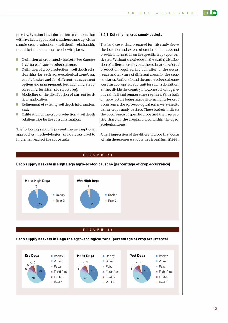
A N E L D A S S E S S M E N T
53
proxies. By using this information in combination with available spatial data, authors came up with a simple crop production – soil depth relationship model by implementing the following tasks:
❚❚ Definition of crop supply baskets (See Chapter 2.4.1) for each agro-ecological zone;
❚❚ Definition of crop production – soil depth rela-tionships for each agro-ecological zone/crop supply basket and for different management options (no management; fertilizer only; struc-tures only; fertilizer and structures);
❚❚ Modelling of the distribution of current ferti-lizer application;
❚❚ Refinement of existing soil depth information, and;
❚❚ Calibration of the crop production – soil depth relationships for the current situation.
The following sections present the assumptions, approaches, methodologies, and datasets used to implement each of the above tasks.
2.4.1 Definition of crop supply baskets
The land cover data prepared for this study shows the location and extent of cropland, but does not provide information on the specific crop types cul-tivated. Without knowledge on the spatial distribu-tion of different crop types, the estimation of crop production required the definition of the occur-rence and mixture of different crops for the crop-land area. Authors found the agro-ecological zones were an appropriate sub-unit for such a definition, as they divide the country into zones of homogene-ous rainfall and temperature regimes. With both of these factors being major determinants for crop occurrence, the agro-ecological zones were used to define crop supply baskets. These baskets indicate the occurrence of specific crops and their respec-tive share on the cropland area within the agro-ecological zone.
A first impression of the different crops that occur within these zones was obtained from Hurni (1998),
F I G U R E 2 5
Crop supply baskets in High Dega agro-ecological zone (percentage of crop occurrence)
95
5
Moist High Dega
Barley
Rest 295
5
Wet High Dega
Barley
Rest 3
40
40
55
5 5
40
40
55
5 5
40
40
55
5 5
Dry Dega Barley
Wheat
Faba
Field Pea
Lentils
Rest 1
Barley
Wheat
Faba
Field Pea
Lentils
Rest 2
Barley
Wheat
Faba
Field Pea
Lentils
Rest 3
Moist Dega Wet DegaF I G U R E 2 6
Crop supply baskets in Dega the agro-ecological zone (percentage of crop occurrence)
95
5
Moist High Dega
Barley
Rest 295
5
Wet High Dega
Barley
Rest 3
40
40
55
5 5
40
40
55
5 5
40
40
55
5 5
Dry Dega Barley
Wheat
Faba
Field Pea
Lentils
Rest 1
Barley
Wheat
Faba
Field Pea
Lentils
Rest 2
Barley
Wheat
Faba
Field Pea
Lentils
Rest 3
Moist Dega Wet Dega
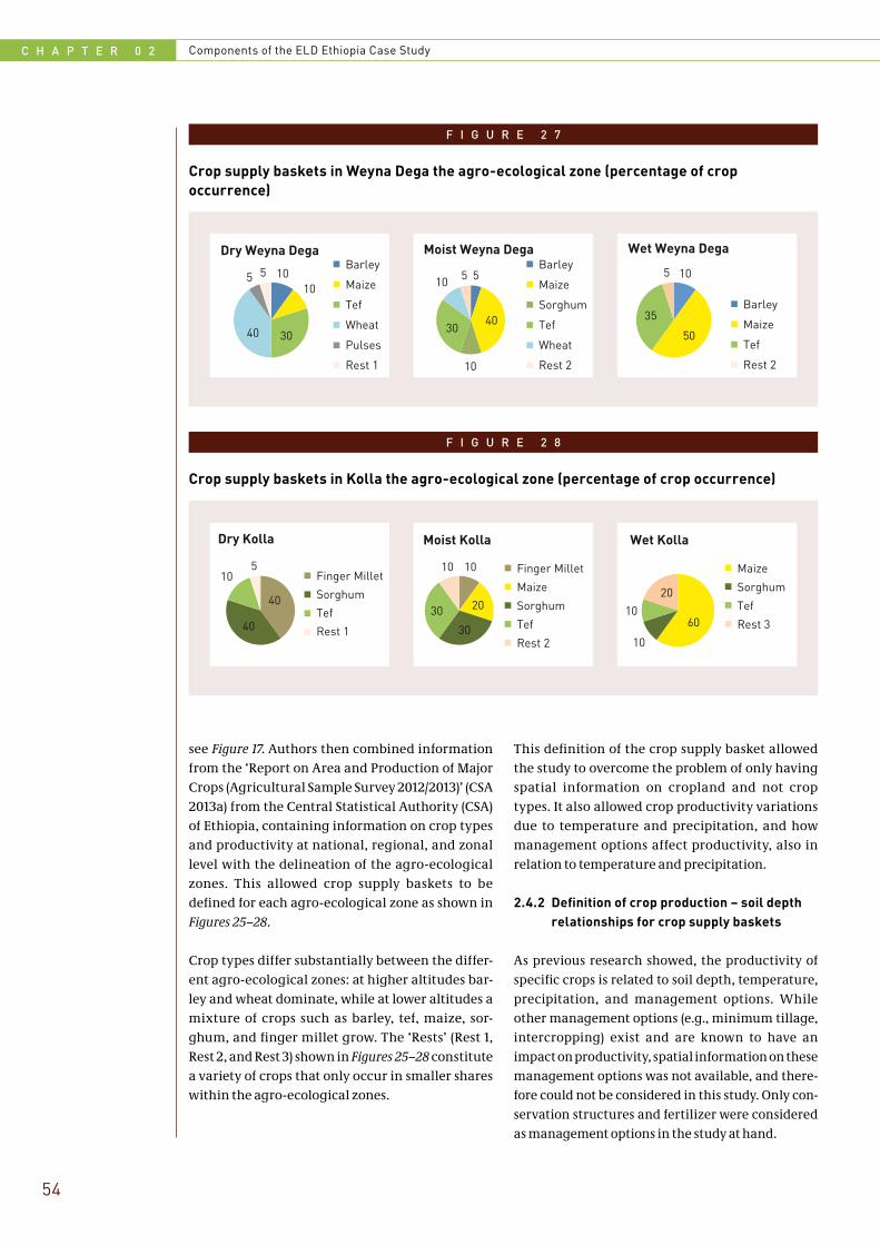
C H A P T E R 0 2 Components of the ELD Ethiopia Case Study
54
F I G U R E 2 7
Crop supply baskets in Weyna Dega the agro-ecological zone (percentage of crop occurrence)
1010
3040
5 5
Dry Weyna DegaBarley
Maize
Tef
Wheat
Pulses
Rest 1
Barley
Maize
Sorghum
Tef
Wheat
Rest 2
Barley
Maize
Tef
Rest 2
5
40
10
30
10 5
Moist Weyna Dega
10
50
35
5
Wet Weyna Dega
40
40
105
Dry Kolla
Finger Millet
Sorghum
Tef
Rest 1
10
20
30
30
10
Moist Kolla
Finger Millet
Maize
Sorghum
Tef
Rest 2
Maize
Sorghum
Tef
Rest 360
10
10
20
Wet KollaF I G U R E 2 8
Crop supply baskets in Kolla the agro-ecological zone (percentage of crop occurrence)
1010
3040
5 5
Dry Weyna DegaBarley
Maize
Tef
Wheat
Pulses
Rest 1
Barley
Maize
Sorghum
Tef
Wheat
Rest 2
Barley
Maize
Tef
Rest 2
5
40
10
30
10 5
Moist Weyna Dega
10
50
35
5
Wet Weyna Dega
40
40
105
Dry Kolla
Finger Millet
Sorghum
Tef
Rest 1
10
20
30
30
10
Moist Kolla
Finger Millet
Maize
Sorghum
Tef
Rest 2
Maize
Sorghum
Tef
Rest 360
10
10
20
Wet Kolla
see Figure 17. Authors then combined information from the ‘Report on Area and Production of Major Crops (Agricultural Sample Survey 2012/2013)’ (CSA 2013a) from the Central Statistical Authority (CSA) of Ethiopia, containing information on crop types and productivity at national, regional, and zonal level with the delineation of the agro-ecological zones. This allowed crop supply baskets to be defined for each agro-ecological zone as shown in Figures 25–28.
Crop types differ substantially between the differ-ent agro-ecological zones: at higher altitudes bar-ley and wheat dominate, while at lower altitudes a mixture of crops such as barley, tef, maize, sor-ghum, and finger millet grow. The ‘Rests’ (Rest 1, Rest 2, and Rest 3) shown in Figures 25–28 constitute a variety of crops that only occur in smaller shares within the agro-ecological zones.
This definition of the crop supply basket allowed the study to overcome the problem of only having spatial information on cropland and not crop types. It also allowed crop productivity variations due to temperature and precipitation, and how management options affect productivity, also in relation to temperature and precipitation.
2.4.2 Definition of crop production – soil depth relationships for crop supply baskets
As previous research showed, the productivity of specific crops is related to soil depth, temperature, precipitation, and management options. While other management options (e.g., minimum tillage, intercropping) exist and are known to have an impact on productivity, spatial information on these management options was not available, and there-fore could not be considered in this study. Only con-servation structures and fertilizer were considered as management options in the study at hand.

A N E L D A S S E S S M E N T
55
Considering precipitation and the management options, crop productivity is affected as shown in Table 8. The productivity ranking (1–4) shows which management options have the highest productivity.
In this ranking, only the dry region shows a differ-ent pattern due to water being the limiting factor: fertilizer can only increase yields substantially when conservation structures exist as they provide better water retention. Although not shown in Table 8, water availability also makes a difference between the productivities of the moist and the wet zones. In the wet zones, management options A and B show similar productivity levels, and options C and D show similar productivity levels. In the moist and wet zones option A is the highest, fol-lowed by options B and C (which show similar pro-ductivity levels) and option D with the lowest pro-ductivity level.
With this relative definition of productivity levels based on precipitation and management options, the study needed to further define absolute levels of productivity for each crop supply basket and management option. This was done using the com-bination of the agro-ecological zones and the ‘Report on Area and Production of Major Crops (Agricultural Sample Survey 2012/2013)’ (Hurni 1998; CSA 2013a). By relating the regional units to the agro-ecological zones with which they overlap, and by grouping crop type information according to the crop supply baskets, the absolute levels of productivity could be defined for each crop supply basket and management option.
Last but not least, crop production – soil depth rela-tionships was defined for each crop supply basket and management options using field measure-ments (SCRP catchments) and the results of the studies of Belay (1992) and Ludi (2002) as references.
2.4.3 Distribution of current fertilizer application
The application of fertilizer has impact on crop pro-ductivity, and thus current fertilizer applications are included in this analysis. To properly calibrate the crop production – soil depths relationships as defined for the crop supply baskets, and for the fol-lowing analyses, authors had to value different management options based on their costs and ben-efits. Unfortunately, there was no spatial data (pixel level) available that showed the current fertilizer applications within the study area. The only source of information that covered the whole study area was the ‘Report on Farm Management Practices’ from the agricultural sample survey of 2012/2013, CSA (2013b), which provided information on the area of cropland treated with UREA and DAP, and the amounts applied at the zonal level.
To transform the zonal level information available to the 30 m x 30 m pixel level that the study model requires, the following assumption was made: fer-tilizer is mainly applied on flat or gentle sloping croplands and on croplands with conservation structures. Fertilizer being a costly investment, it is less likely that farmers would apply it on croplands that have steep slopes because erosion rates on such lands are high, washing away the fertilizer in the absence of erosion reduction strategies on such croplands.
Fertilizer distribution was then implemented in the model in the following way: the amount of cropland treated with fertilizer for each zone was combined with pixel based slope information. The fertilizer was then redistributed within these zone-slope-cropland areas. Non-sloping croplands were to be treated with fertilizer (sloping croplands with conservation structures were also considered in
T A B L E 8
Productivity levels of crops according to precipitation and management option(1 stands for highest and 4 for lowest ranking)
Dry Moist Wet
A) Conservation structures/fertilizer 1 1 1
B) Fertilizer only 3 2 2
C) Conservation structures only 2 3 3
D) No management 4 4 4
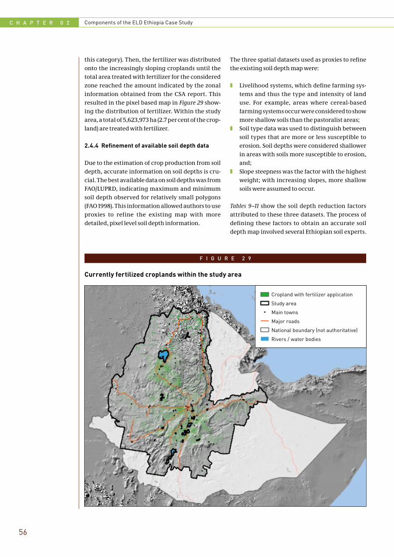
C H A P T E R 0 2 Components of the ELD Ethiopia Case Study
56
this category). Then, the fertilizer was distributed onto the increasingly sloping croplands until the total area treated with fertilizer for the considered zone reached the amount indicated by the zonal information obtained from the CSA report. This resulted in the pixel based map in Figure 29 show-ing the distribution of fertilizer. Within the study area, a total of 5,623,973 ha (2.7 per cent of the crop-land) are treated with fertilizer.
2.4.4 Refinement of available soil depth data
Due to the estimation of crop production from soil depth, accurate information on soil depths is cru-cial. The best available data on soil depths was from FAO/LUPRD, indicating maximum and minimum soil depth observed for relatively small polygons (FAO 1998). This information allowed authors to use proxies to refine the existing map with more detailed, pixel level soil depth information.
The three spatial datasets used as proxies to refine the existing soil depth map were:
❚❚ Livelihood systems, which define farming sys-tems and thus the type and intensity of land use. For example, areas where cereal-based farming systems occur were considered to show more shallow soils than the pastoralist areas;
❚❚ Soil type data was used to distinguish between soil types that are more or less susceptible to erosion. Soil depths were considered shallower in areas with soils more susceptible to erosion, and;
❚❚ Slope steepness was the factor with the highest weight; with increasing slopes, more shallow soils were assumed to occur.
Tables 9–11 show the soil depth reduction factors attributed to these three datasets. The process of defining these factors to obtain an accurate soil depth map involved several Ethiopian soil experts.
F I G U R E 2 9
Currently fertilized croplands within the study area
!
Cropland with fertilizer application
Study area
Main towns
Major roads
National boundary (not authoritative)
Rivers / water bodies
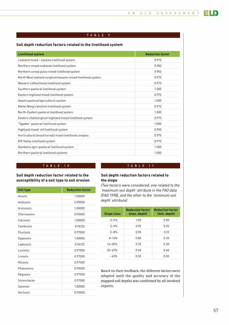
A N E L D A S S E S S M E N T
57
T A B L E 9
T A B L E 1 0
Soil depth reduction factors related to the livelihood system
Soil depth reduction factor related to the susceptibility of a soil type to soil erosion
Livelihood system Reduction factor
Lowland mixed – sesame livelihood system 0.975
Northern mixed midlands livelihood system 0.950
Northern cereal pulse mixed livelihood system 0.950
North West lowland sorghum/sesame mixed livelihood system 0.975
Western coffee/maize livelihood system 0.975
Southern pastoral livelihood system 1.000
Eastern highland mixed livelihood system 0.975
Awash pastoral/agricultural system 1.000
Meher/Belg transition livelihood system 0.975
North-Eastern pastoral livelihood system 1.000
Eastern chat/sorghum highland mixed livelihood system 0.975
“Ogaden” pastoral livelihood system 1.000
Highland mixed -tef livelihood system 0.950
Horticultural (enset/cereal) mixed livelihood complex 0.975
Rift Valley livelihood system 0.975
Gambella agro-pastoral livelihood system 1.000
Northern pastoral livelihood systems 1.000
Soil type Reduction factor
Alisols 1.00000
Andosols 0.95000
Arenosols 1.00000
Chernozems 0.95000
Calcisols 1.00000
Cambisols 0.96125
Fluvisols 0.97000
Gypsisols 1.00000
Leptosols 0.96125
Luvisols 0.97500
Lixisols 0.97500
Nitisols 0.97500
Phaeozems 0.95000
Regosols 0.97500
Solonchacks 0.97500
Solonetz 1.00000
Vertisols 0.95000
T A B L E 1 1
Soil depth reduction factors related to the slope(Two factors were considered, one related to the ‘maximum soil depth’ attribute in the FAO data [FAO 1998], and the other to the ‘minimum soil depth’ attribute)
Slope classReduction factor
(max. depth)Reduction factor
(min. depth)
0–2% 1.00 0.00
2–5% 0.95 0.05
5–8% 0.90 0.10
8–16% 0.80 0.20
16–30% 0.70 0.30
30–45% 0.60 0.40
› 45% 0.50 0.50
Based on their feedback, the different factors were adapted until the quality and accuracy of the mapped soil depths was confirmed by all involved experts.
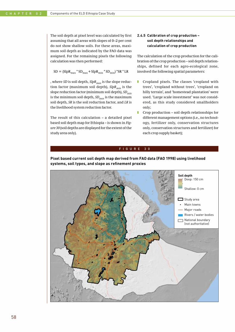
C H A P T E R 0 2 Components of the ELD Ethiopia Case Study
58
The soil depth at pixel level was calculated by first assuming that all areas with slopes of 0–2 per cent do not show shallow soils. For these areas, maxi-mum soil depth as indicated by the FAO data was assigned. For the remaining pixels the following calculation was then performed:
SD = (SlpRmax * SDmax + SlpRmin * SDmin) *SR * LR
, where SD is soil depth, SlpRmax is the slope reduc-tion factor (maximum soil depth), SlpRmin is the slope reduction factor (minimum soil depth), SDmin is the minimum soil depth, SDmax is the maximum soil depth, SR is the soil reduction factor, and LR is the livelihood system reduction factor.
The result of this calculation – a detailed pixel based soil depth map for Ethiopia – is shown in Fig-ure 30 (soil depths are displayed for the extent of the study area only).
2.4.5 Calibration of crop production – soil depth relationships and calculation of crop production
The calculation of the crop production for the cali-bration of the crop production – soil depth relation-ships, defined for each agro-ecological zone, involved the following spatial parameters:
❚❚ Cropland pixels. The classes ‘cropland with trees’, ‘cropland without trees’, ‘cropland on hilly terrain’, and ‘homestead plantation’ were used. ‘Large scale investment’ was not consid-ered, as this study considered smallholders only;
❚❚ Crop production – soil depth relationships for different management options (i.e., no technol-ogy, fertilizer only, conservation structures only, conservation structures and fertilizer) for each crop supply basket);
F I G U R E 3 0
Pixel based current soil depth map derived from FAO data (FAO 1998) using livelihood systems, soil types, and slope as refinement proxies
!
Soil depthDeep: 150 cm
Shallow: 0 cm
Study area
Main towns
Major roads
Rivers / water bodies
National boundary(not authoritative)
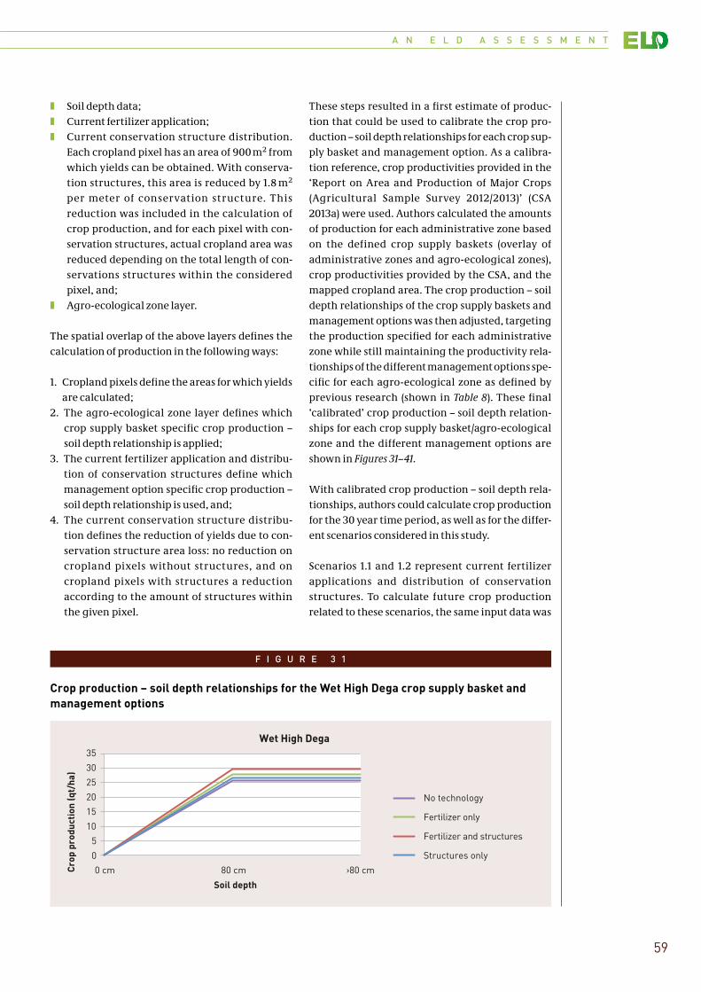
A N E L D A S S E S S M E N T
59
❚❚ Soil depth data;❚❚ Current fertilizer application;❚❚ Current conservation structure distribution.
Each cropland pixel has an area of 900 m2 from which yields can be obtained. With conserva-tion structures, this area is reduced by 1.8 m2
per meter of conser vat ion st r uct ure. T his reduction was included in the calculation of crop production, and for each pixel with con-servation structures, actual cropland area was reduced depending on the total length of con-servations structures within the considered pixel, and;
❚❚ Agro-ecological zone layer.
The spatial overlap of the above layers defines the calculation of production in the following ways:
1. Cropland pixels define the areas for which yields are calculated;
2. The agro-ecological zone layer defines which crop supply basket specific crop production – soil depth relationship is applied;
3. The current fertilizer application and distribu-tion of conservation structures define which management option specific crop production – soil depth relationship is used, and;
4. The current conservation structure distribu-tion defines the reduction of yields due to con-servation structure area loss: no reduction on cropland pixels without structures, and on cropland pixels with structures a reduction according to the amount of structures within the given pixel.
These steps resulted in a first estimate of produc-tion that could be used to calibrate the crop pro-duction – soil depth relationships for each crop sup-ply basket and management option. As a calibra-tion reference, crop productivities provided in the ‘Report on Area and Production of Major Crops (Agricultural Sample Survey 2012/2013)’ (CSA 2013a) were used. Authors calculated the amounts of production for each administrative zone based on the defined crop supply baskets (overlay of administrative zones and agro-ecological zones), crop productivities provided by the CSA, and the mapped cropland area. The crop production – soil depth relationships of the crop supply baskets and management options was then adjusted, targeting the production specified for each administrative zone while still maintaining the productivity rela-tionships of the different management options spe-cific for each agro-ecological zone as defined by previous research (shown in Table 8). These final ‘calibrated’ crop production – soil depth relation-ships for each crop supply basket/agro-ecological zone and the different management options are shown in Figures 31–41.
With calibrated crop production – soil depth rela-tionships, authors could calculate crop production for the 30 year time period, as well as for the differ-ent scenarios considered in this study.
Scenarios 1.1 and 1.2 represent current fertilizer applications and distribution of conservation structures. To calculate future crop production related to these scenarios, the same input data was
F I G U R E 3 1
Crop production – soil depth relationships for the Wet High Dega crop supply basket and management options
0
5
10
15
20
25
30
35
0 cm 80 cm ›80 cmCro
p pr
oduc
tion
(qt/
ha)
Soil depth
No technology
Fertilizer only
Fertilizer and structures
Structures only
Wet High Dega
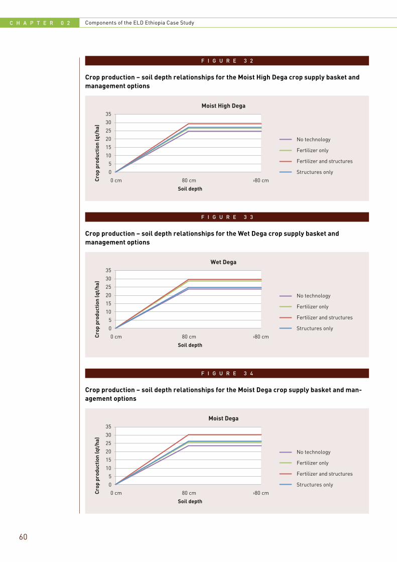
C H A P T E R 0 2 Components of the ELD Ethiopia Case Study
60
F I G U R E 3 2
Crop production – soil depth relationships for the Moist High Dega crop supply basket and management options
0
5
10
15
20
25
30
35
0 cm 80 cm ›80 cmCro
p pr
oduc
tion
(qt/
ha)
Soil depth
No technology
Fertilizer only
Fertilizer and structures
Structures only
Moist High Dega
F I G U R E 3 3
Crop production – soil depth relationships for the Wet Dega crop supply basket and management options
0
5
10
15
20
25
30
35
0 cm 80 cm ›80 cmCro
p pr
oduc
tion
(qt/
ha)
Soil depth
No technology
Fertilizer only
Fertilizer and structures
Structures only
Wet Dega
F I G U R E 3 4
Crop production – soil depth relationships for the Moist Dega crop supply basket and man-agement options
0
5
10
15
20
25
30
35
0 cm 80 cm ›80 cmCro
p pr
oduc
tion
(qt/
ha)
Soil depth
No technology
Fertilizer only
Fertilizer and structures
Structures only
Moist Dega
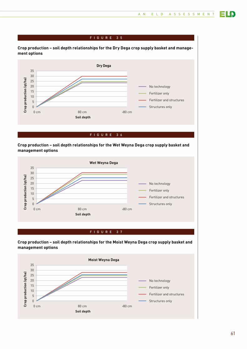
A N E L D A S S E S S M E N T
61
F I G U R E 3 5
Crop production – soil depth relationships for the Dry Dega crop supply basket and manage-ment options
0
5
10
15
20
25
30
35
0 cm 80 cm ›80 cmCro
p pr
oduc
tion
(qt/
ha)
Soil depth
No technology
Fertilizer only
Fertilizer and structures
Structures only
Dry Dega
F I G U R E 3 6
Crop production – soil depth relationships for the Wet Weyna Dega crop supply basket and management options
0
5
10
15
20
25
30
35
0 cm 80 cm ›80 cmCro
p pr
oduc
tion
(qt/
ha)
Soil depth
No technology
Fertilizer only
Fertilizer and structures
Structures only
Wet Weyna Dega
F I G U R E 3 7
Crop production – soil depth relationships for the Moist Weyna Dega crop supply basket and management options
0
5
10
15
20
25
30
35
0 cm 80 cm ›80 cmCro
p pr
oduc
tion
(qt/
ha)
Soil depth
No technology
Fertilizer only
Fertilizer and structures
Structures only
Moist Weyna Dega
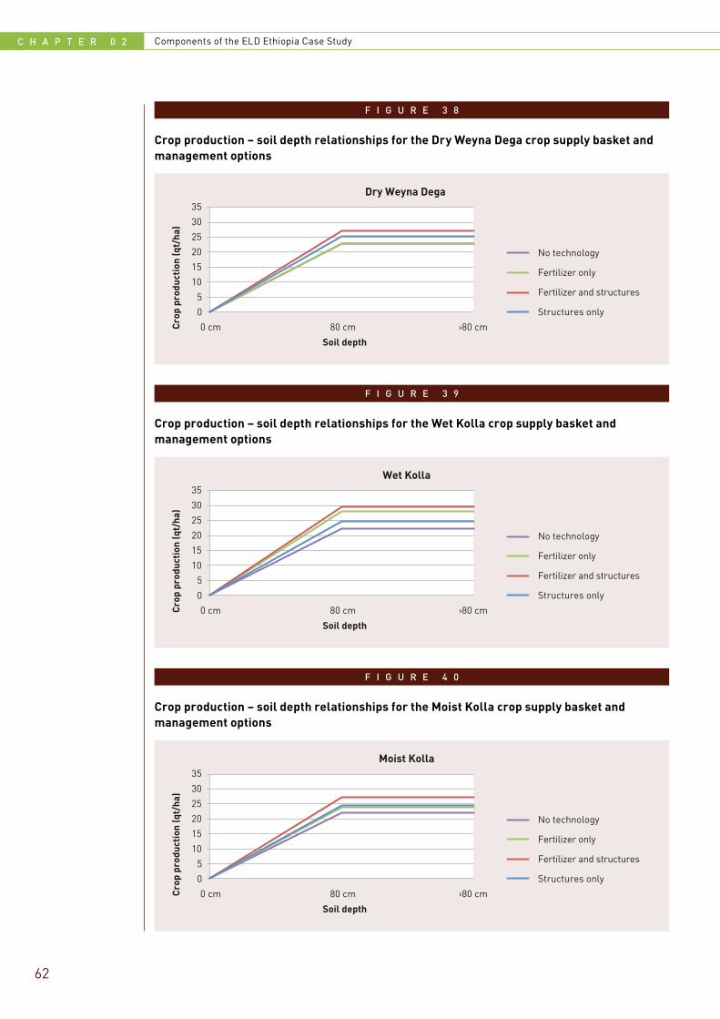
C H A P T E R 0 2 Components of the ELD Ethiopia Case Study
62
F I G U R E 3 8
Crop production – soil depth relationships for the Dry Weyna Dega crop supply basket and management options
0
5
10
15
20
25
30
35
0 cm 80 cm ›80 cmCro
p pr
oduc
tion
(qt/
ha)
Soil depth
No technology
Fertilizer only
Fertilizer and structures
Structures only
Dry Weyna Dega
F I G U R E 3 9
Crop production – soil depth relationships for the Wet Kolla crop supply basket and management options
0
5
10
15
20
25
30
35
0 cm 80 cm ›80 cmCro
p pr
oduc
tion
(qt/
ha)
Soil depth
No technology
Fertilizer only
Fertilizer and structures
Structures only
Wet Kolla
F I G U R E 4 0
Crop production – soil depth relationships for the Moist Kolla crop supply basket and management options
0
5
10
15
20
25
30
35
0 cm 80 cm ›80 cmCro
p pr
oduc
tion
(qt/
ha)
Soil depth
No technology
Fertilizer only
Fertilizer and structures
Structures only
Moist Kolla
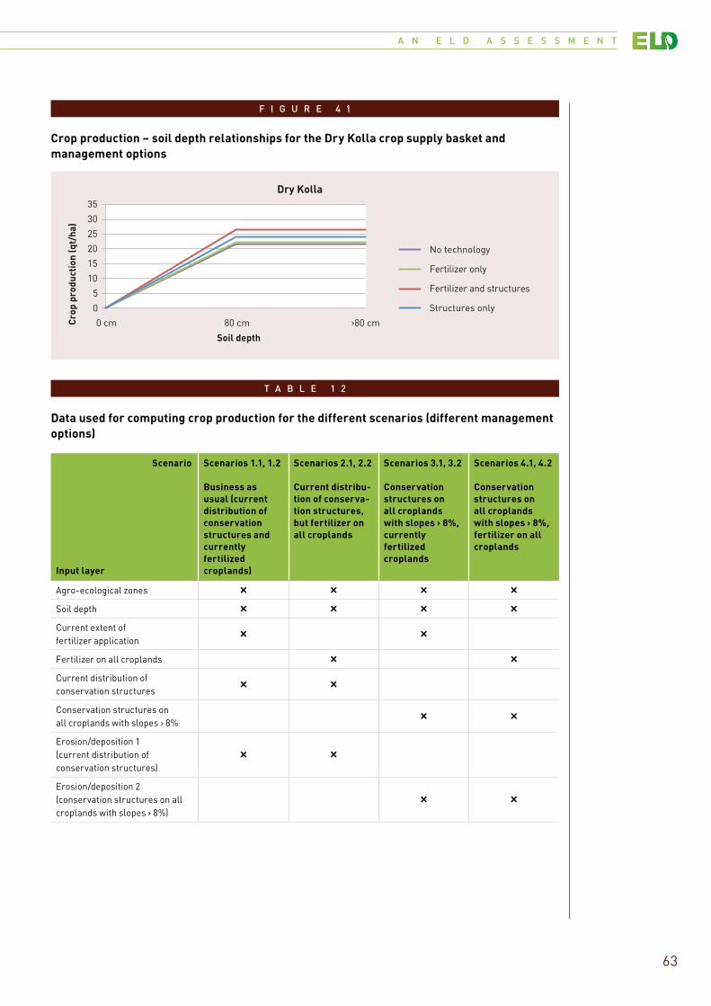
A N E L D A S S E S S M E N T
63
F I G U R E 4 1
Crop production – soil depth relationships for the Dry Kolla crop supply basket and management options
0
5
10
15
20
25
30
35
0 cm 80 cm ›80 cmCro
p pr
oduc
tion
(qt/
ha)
Soil depth
No technology
Fertilizer only
Fertilizer and structures
Structures only
Dry Kolla
T A B L E 1 2
Data used for computing crop production for the different scenarios (different management options)
Scenario Input layer
Scenarios 1.1, 1.2 Business as usual (current distribution of conservation structures and currently fertilized croplands)
Scenarios 2.1, 2.2 Current distribu-tion of conserva-tion structures, but fertilizer on all croplands
Scenarios 3.1, 3.2 Conservation structures on all croplands with slopes › 8%, currently fertilized croplands
Scenarios 4.1, 4.2 Conservation structures on all croplands with slopes › 8%, fertilizer on all croplands
Agro-ecological zones l l l l
Soil depth l l l l
Current extent of fertilizer application
l l
Fertilizer on all croplands l l
Current distribution of conservation structures
l l
Conservation structures on all croplands with slopes › 8%
l l
Erosion/deposition 1 (current distribution of conservation structures)
l l
Erosion/deposition 2 (conservation structures on all croplands with slopes › 8%)
l l
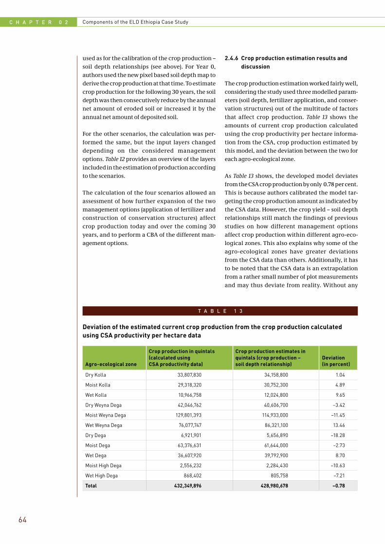
C H A P T E R 0 2 Components of the ELD Ethiopia Case Study
64
used as for the calibration of the crop production – soil depth relationships (see above). For Year 0, authors used the new pixel based soil depth map to derive the crop production at that time. To estimate crop production for the following 30 years, the soil depth was then consecutively reduce by the annual net amount of eroded soil or increased it by the annual net amount of deposited soil.
For the other scenarios, the calculation was per-formed the same, but the input layers changed depending on the considered management options. Table 12 provides an overview of the layers included in the estimation of production according to the scenarios.
The calculation of the four scenarios allowed an assessment of how further expansion of the two management options (application of fertilizer and construction of conservation structures) affect crop production today and over the coming 30 years, and to perform a CBA of the different man-agement options.
2.4.6 Crop production estimation results and discussion
The crop production estimation worked fairly well, considering the study used three modelled param-eters (soil depth, fertilizer application, and conser-vation structures) out of the multitude of factors that affect crop production. Table 13 shows the amounts of current crop production calculated using the crop productivity per hectare informa-tion from the CSA, crop production estimated by this model, and the deviation between the two for each agro-ecological zone.
As Table 13 shows, the developed model deviates from the CSA crop production by only 0.78 per cent. This is because authors calibrated the model tar-geting the crop production amount as indicated by the CSA data. However, the crop yield – soil depth relationships still match the findings of previous studies on how different management options affect crop production within different agro-eco-logical zones. This also explains why some of the agro-ecological zones have greater deviations from the CSA data than others. Additionally, it has to be noted that the CSA data is an extrapolation from a rather small number of plot measurements and may thus deviate from reality. Without any
T A B L E 1 3
Deviation of the estimated current crop production from the crop production calculated using CSA productivity per hectare data
Agro-ecological zone
Crop production in quintals (calculated using CSA productivity data)
Crop production estimates in quintals (crop production – soil depth relationship)
Deviation (in percent)
Dry Kolla 33,807,830 34,158,800 1.04
Moist Kolla 29,318,320 30,752,300 4.89
Wet Kolla 10,966,758 12,024,800 9.65
Dry Weyna Dega 42,046,762 40,606,700 –3.42
Moist Weyna Dega 129,801,393 114,933,000 –11.45
Wet Weyna Dega 76,077,747 86,321,100 13.46
Dry Dega 6,921,901 5,656,890 –18.28
Moist Dega 63,376,631 61,644,000 –2.73
Wet Dega 36,607,920 39,792,900 8.70
Moist High Dega 2,556,232 2,284,430 –10.63
Wet High Dega 868,402 805,758 –7.21
Total 432,349,896 428,980,678 –0.78
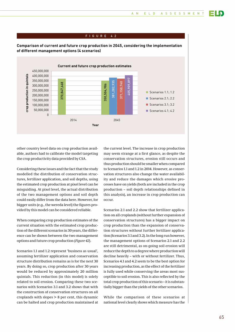
A N E L D A S S E S S M E N T
65
other country level data on crop production avail-able, authors had to calibrate the model targeting the crop productivity data provided by CSA.
Considering these issues and the fact that the study modelled the distribution of conservation struc-tures, fertilizer application, and soil depths, using the estimated crop production at pixel level can be misguiding. At pixel level, the actual distribution of the two management options and soil depth could easily differ from the data here. However, for bigger units (e.g., the wereda level) the figures pro-vided by this model can be considered reliable.
When comparing crop production estimates of the current situation with the estimated crop produc-tion of the different scenarios in 30 years, the differ-ence can be shown between the two management options and future crop production (Figure 42).
Scenarios 1.1 and 1.2 represent 'business as usual’, assuming fertilizer application and conservation structure distribution remains as is for the next 30 years. By doing so, crop production after 30 years would be reduced by approximately 20 million quintals. This reduction (in this model) is solely related to soil erosion. Comparing these two sce-narios with Scenarios 3.1 and 3.2 shows that with the construction of conservation structures on all croplands with slopes > 8 per cent, this dynamic can be halted and crop production maintained at
the current level. The increase in crop production may seem strange at a first glance, as despite the conservation structures, erosion still occurs and thus production should be smaller when compared to Scenarios 1.1 and 1.2 in 2014. However, as conser-vation structures also change the water availabil-ity and reduce the damages which erosive pro-cesses have on yields (both are included in the crop production – soil depth relationships defined in this analysis), an increase in crop production can occur.
Scenarios 2.1 and 2.2 show that fertilizer applica-tion on all croplands (without further expansion of conservation structures) has a bigger impact on crop production than the expansion of conserva-tion structures without further fertilizer applica-tion (Scenarios 3.1 and 3.2). In the long run however, the management options of Scenarios 2.1 and 2.2 are still detrimental, as on-going soil erosion will reduce the depth to a degree where production will decline heavily – with or without fertilizer. Thus, Scenarios 4.1 and 4.2 seem to be the best option for increasing production, as the effect of the fertilizer is fully used while conserving the areas most sus-ceptible to soil erosion. This is also reflected by the total crop production of this scenario – it is substan-tially bigger than the yields of the other scenarios.
While the comparison of these scenarios at national level clearly shows which measure has the
F I G U R E 4 2
Comparison of current and future crop production in 2045, considering the implementation of different management options (4 scenarios)
370,847,668
350,504,986
381,282,935
371,150,740
405,909,897
0
50,000,000
100,000,000
150,000,000
200,000,000
250,000,000
300,000,000
350,000,000
400,000,000
450,000,000
2014 2045
crop
pro
duct
ion
in q
uint
als
Year
Current and future crop production estimates
Scenarios 1.1; 1.2
Scenarios 2.1; 2.2
Scenarios 3.1; 3.2
Scenarios 4.1; 4.2
C H A P T E R 0 2 Components of the ELD Ethiopia Case Study
66
biggest potential for increasing future crop pro-duction, it may not be the most beneficial choice in all areas, nor the most beneficial in economic terms. In order to find out which scenario brings the biggest economic benefit, a CBA (one of the main ways that economists use to analyse major development proposals and environmental prob-lems) was performed for each at pixel level.
2.5 Component 5: Financial Cost-Benefit Analysis (CBA)
An understanding of the factors that may influence farmers in making investments in SLM technolo-gies allows policy-makers to design policies more effectively. Without sufficient profitability, other factors that condition adoption become less rele-vant. A financial cost-benefit analysis is used to evaluate the profitability of SLM investment under various scenarios. The objective of a CBA is to com-pare the present value of the stream of benefits (pos-itive effects) and the present value of all investments and recurrent costs (negative effects). A CBA can either be carried out from the farmers’ perspective (financial CBA) or society as a whole (economic and social CBA). In this case, authors considered the for-mer as benefits to society as a whole (e.g., off-site impacts of soil erosion) were not considered due to limited availability of spatially explicit data.
A CBA has the following components: determina-tion of evaluation criteria; identification of effects (costs and benefits); quantification in physical terms of the effects; valuation of effects; determination of time horizon; weighing of the costs and benefits in time (discounting) and sensitivity analysis (de Graaff, 1996). The most commonly used CBA evalua-tion criteria are the benefit/cost ratio (B/C ratio), the net present value (NPV) and the internal rate of return (IRR). For this study, NPV and IRR are used as evaluation criteria. If the NPV is positive, it means the investment on SLM measures was profitable. However, if NPV is negative, the costs outweigh the benefits benefits, meaning that the investments in SLM measures were not economical. Similarly, if the IRR is greater than the existing opportunity cost of capital (discount rate), then investment on SLM measures is acceptable, and otherwise not. In the financial CBA, a discount rate of 12.5% (NBE 2014) and a lifetime of 30 years are assumed.
Due to the uncertainty in the value of some param-eters (e.g., prices and costs) a sensitivity analysis was carried out to test the robustness of the outcome of the financial cost-benefit analysis.
Although most important parameters used in the analysis are carefully computed and validated, this CBA had the following limitations:
1) Due to a lack of pixel or village specific informa-tion, most parameters (e.g. prices of inputs and crops, amount of fertilizer use) considered in the analysis are average parameters obtained either at provincial, regional, or national level;
2) As the distribution of SLM investments/conser-vation structures was modeled, the costs and benefits associated for each structure type were not computed, instead average costs and bene-fits were used in the analysis, and;
3) The CBA mainly focused on direct and measura-ble benefits (crop production change due to SLM investments) but other private benefits (e.g., crop residue due to change in crop production and other associated benefits) and societal ben-efits are not included in the analysis. These omis-sions will underestimate the benefits of invest-ments in SLM.
These limitations suggest that caution is needed in interpretation of results.
2.5.1 Data preparation for the CBA at pixel level
The CBA was performed for the eight different sce-narios described below to determine the most prof-itable scenario at pixel level, and considering the limitations faced at pixel level, also for clusters of pixels and administrative units. For each of the parameters included in the different scenarios (Table 14), authors attributed the costs and the ben-efits in Ethiopian Birr (ETB). The following scenar-ios were considered.
❚❚ Scenario 1.1: CBA including the distribution of currently existing conservation structures and the currently fertilized croplands. This sce-nario represents “business as usual” or a base-line scenario, as no additional investments are considered;
A N E L D A S S E S S M E N T
67
❚❚ Scenario 1.2: Equivalent to Scenario 1.1, but including the costs and benefits of planting fod-der grass on the conservation structures;
❚❚ Scenario 2.1: CBA including the distribution of current conservation structures and assuming the application of fertilizer on all croplands;
❚❚ Scenario 2.2: Equivalent to Scenario 2.1, but including the costs and benefits of planting fod-der grass on the conservation structures;
❚❚ Scenario 3.1: CBA including the distribution of current conservation structures, assuming the additional construction of conservation struc-tures on all croplands with slopes > 8 per cent, and the currently fertilized croplands;
❚❚ Scenario 3.2: Equivalent to Scenario 3.1, but including the costs and benefits of planting fod-der grass on the conservation structures (exist-ing and new);
❚❚ Scenario 4.1: CBA including the distribution of current conservation structures, assuming the additional construction of conservation struc-tures on all croplands with slopes > 8 per cent, and assuming the application of fertilizer on all croplands, and;
❚❚ Scenario 4.2: Equivalent to Scenario 4.1, but including the costs and benefits of planting fod-der grass on the conservation structures (exist-ing and new).
Table 14 shows an overview of the scenarios and parameters involved. From Scenario 1.1 to Scenario 4.2, incremental change in the benefits and costs related to the adoption of conservation structures are considered. The following sections then describe how the costs and benefits for each of the parameters were measured.
Crop production benefits
The crop production estimation in this study (described in the previous chapter) already included some of the costs and benefits related to the different management options. For example, estimates already reflect the biophysical benefits from applying fertilizer, of increased water availa-bility and crop production reduction because of cropland area loss due to conservation structures, and decline in soil depth related to erosion (or increase in crop production due to the increase in soil depth related to deposition). With these effects already included in production, implementing the financial CBA at pixel level was less complex as the
benefits from production and applied manage-ment options could be directly calculated from the amount of crop production. Only fertilizer costs, construction/maintenance costs related to the con-servation structures, and nutrient depletion of soils due to the enrichment ratio were considered as additional costs in the financial CBA.
Two crop prices sources were used to attribute a monetary value to the crop production:
❚❚ Average retail prices of crops for 84 market loca-tions distributed across various regions consid-ered, obtained from the CSA ‘Annual average retail prices of goods and services July 2012 – June 2013’ (CSA 2013c), and;
❚❚ Average farm gate prices for the different zones in January 2013 (CSA 2014).
The first dataset provides point locations with aver-age retail prices, which allows attributing crop prices to the agro-ecological zones for which the crop supply baskets were defined. However, aver-age retail prices do not represent farm gate prices, as they include additional costs and benefits until the product reaches the final consumers. The sec-ond dataset provides farm gate prices, but at the zonal level, which makes the attributing to the agro-ecological zones/crop supply baskets more difficult. The prices for crop supply baskets were therefore assessed the following way:
1. Assessing the mean difference between the aver-age retail prices and the farm gate prices by com-paring the point data average retail prices within a specific administrative zone with the farm gate prices of that zone. This allowed for the adjustment of the point data average retail prices by the mean difference assessed to obtain farm gate prices;
2. Calculating average farm gate prices from adjusted average retail price point data for each agro-ecological zone, and;
3. Defining the price for one kg of crop yield for each crop supply basket based on the summa-rized price information per agro-ecological zone and the percentage of crop occurrence defined by the crop supply basket.
Once the price for each crop supply basket defined 1, the yield benefits for each scenario and year could be computed at pixel level.
1 Crop basket prices are derived from 2012/2013 average retail and farm gate prices
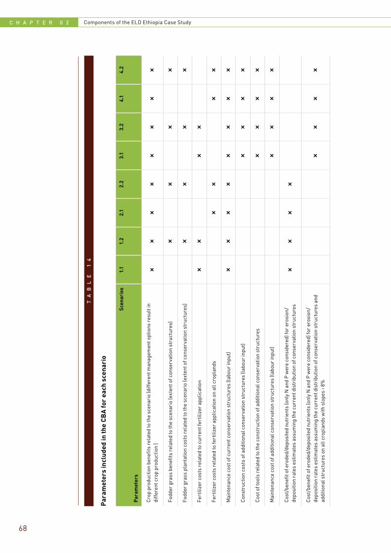
C H A P T E R 0 2 Components of the ELD Ethiopia Case Study
68
TA
BL
E
14
Par
amet
ers
incl
uded
in th
e C
BA
for
each
sce
nari
o
Scen
ario
s
Par
amet
ers
1.1
1.2
2.1
2.2
3.1
3.2
4.1
4.2
Cro
p pr
oduc
tion
bene
fits
rela
ted
to th
e sc
enar
io (d
iffer
ent m
anag
emen
t opt
ions
res
ult i
n di
ffer
ent c
rop
prod
uctio
n )
ll
ll
ll
ll
Fodd
er g
rass
ben
efits
rel
ated
to th
e sc
enar
io (e
xten
t of c
onse
rvat
ion
stru
ctur
es)
ll
ll
Fodd
er g
rass
pla
ntat
ion
cost
s re
late
d to
the
scen
ario
(ext
ent o
f con
serv
atio
n st
ruct
ures
)l
ll
l
Fert
ilize
r co
sts
rela
ted
to c
urre
nt fe
rtili
zer
appl
icat
ion
ll
ll
Fert
ilize
r co
sts
rela
ted
to fe
rtili
zer
appl
icat
ion
on a
ll cr
opla
nds
ll
ll
Mai
nten
ance
cos
t of c
urre
nt c
onse
rvat
ion
stru
ctur
es (l
abou
r in
put)
ll
ll
ll
ll
Con
stru
ctio
n co
sts
of a
dditi
onal
con
serv
atio
n st
ruct
ures
(lab
our
inpu
t)l
ll
l
Cos
t of t
ools
rel
ated
to th
e co
nstr
uctio
n of
add
ition
al c
onse
rvat
ion
stru
ctur
esl
ll
l
Mai
nten
ance
cos
t of a
dditi
onal
con
serv
atio
n st
ruct
ures
(lab
our
inpu
t)l
ll
l
Cos
t/be
nefit
of e
rode
d/de
posi
ted
nutr
ient
s (o
nly
N a
nd P
wer
e co
nsid
ered
) for
ero
sion
/de
posi
tion
rate
s es
timat
es a
ssum
ing
the
curr
ent d
istr
ibut
ion
of c
onse
rvat
ion
stru
ctur
esl
ll
l
Cos
t/be
nefit
of e
rode
d/de
posi
ted
nutr
ient
s (o
nly
N a
nd P
wer
e co
nsid
ered
) for
ero
sion
/de
posi
tion
rate
s es
timat
es a
ssum
ing
the
curr
ent d
istr
ibut
ion
of c
onse
rvat
ion
stru
ctur
es a
nd
addi
tiona
l str
uctu
res
on a
ll cr
opla
nds
with
slo
pes
› 8%
ll
ll
A N E L D A S S E S S M E N T
69
Fertilizer costs
The ‘Report on Farm Management Practices’ from the CSA agricultural sample survey of 2012/2013 (2013b), was used to define the croplands treated with fertilizer for each administrative zone, and also provides information on the amounts of ferti-lizer (UREA and DAP, although no information on the shares of each) applied. This allowed authors to calculate the amounts of fertilizer used on each pixel where it is applied. Without information on the respective shares of UREA and DAP, the study calculated the price for one kg of fertilizer from the national average prices (Shahidur et al. 2012). This resulted in a fertilizer price of 14.64 ETB per kg2, which is a rather rough estimate as the same share of UREA and DAP is not necessarily used.
For Scenarios 1.1, 1.2, 3.1, and 3.2, authors could cal-culate fertilizer cost for each pixel by multiplying the amount applied (in kg) by 14.64 ETB.
For Scenarios 2.1, 2.2, 4.1, and 4.2 (application of fer-tilizer on all croplands) it was assumed that same amount of fertilizer is applied on ‘new’ pixels as on the cropland pixels currently treated with ferti-lizer, within each administrative zone. Consider-ing that current fertilizer use is below the opti-mum, these scenarios may not show the optimal situation/yields that could be obtained when apply-ing fertilizer as recommended by research. Thus crop production estimates were calibrated consid-ering current fertilizer application. Without know-ing how optimal fertilizer use affects yields, the study assumed that fertilizer amounts applied on all cropland pixels are the same as on the cropland pixels currently treated with fertilizer, otherwise, it would not be possible to properly estimate the yields. The fertilizer cost of these scenarios was cal-culated the same way as above, by multiplying the amount of fertilizer applied by 14.64 ETB.
Conservation structure costs
Several costs are related to the building of conser-vation structures: construction costs, maintenance costs, and the cost of tools. Although different types of structures (soil bund, fanya juu bund, and ter-races) have different costs, average construction and maintenance costs were considered because the distribution of conservation structures was modelled, authors were not able to distinguish costs by type of structure.
From the conservation structure distribution model, the length of conservation structures in meters per pixel could be extracted and used to cal-culate the cost per pixel. As the construction and maintenance is often done during off-season, their costs relate to off-season rural wages (Lakew et al. 2005), which vary across the study area. However, authors did not find sufficient information to model these variations and SLM experts were thus consulted to obtain an estimate. Based on this a national daily wage rate of 40 ETB in 2013 was assumed to compute the following costs3:
❚❚ Construction costs: 5 m of structures/day at 40 ETB/day (8 ETB/m of structure)
❚❚ Maintenance cost: 50 m of structures/day at 40 ETB/day (0.8 ETB/m of structure)
❚❚ Cost of tools: 200 ETB/1000 m of structures (0.2 ETB/m of structure)
While the construction costs (tools and labour) are one-time, maintenance of the structures has to be performed on an annual basis over 15 years until they are stabilized. As the different scenarios only considered existing structures (Scenarios 1.1, 1.2, 2.1, and 2.2) or both existing and new (Scenarios 3.1, 3.2, 4.1, and 4.2), different costs related to the con-servation structures had to be considered for differ-ent scenarios.
For Scenarios 1.1, 1.2, 2.1, and 2.2 (only considering existing structures) only maintenance costs (labour based on the metres of structures per year) over 5 years were included in the CBA. As the struc-tures already existed, no construction costs were applied. Additionally authors did not know the age of the specific structures, so they were assumed to be 10 years of age and only needing maintenance for another 5 years.
For Scenarios 3.1, 3.2, 4.1, and 4.2 (existing and new structures), a maintenance cost over 5 years was assumed for the existing structures. For the new structures the one-time construction costs (labour and tools based on the meters of structures per pixel) were assumed to be in the first year, and the mainte-nance costs (labour per meter of structure per pixel) started in the second year, lasting for 15 years.
2 UREA and DAP prices from 2012 ac-cording to Shahidur et al. 2012. Due to the high variability of the prices over the years according to Shahidur et al. 2012, adjustments for inflation for the price in 2013 were not performed; prices are representative only.
3 Due to spatial vari-ability and lack of data costs are expert-based estimates and rather representative than spatially accurate.
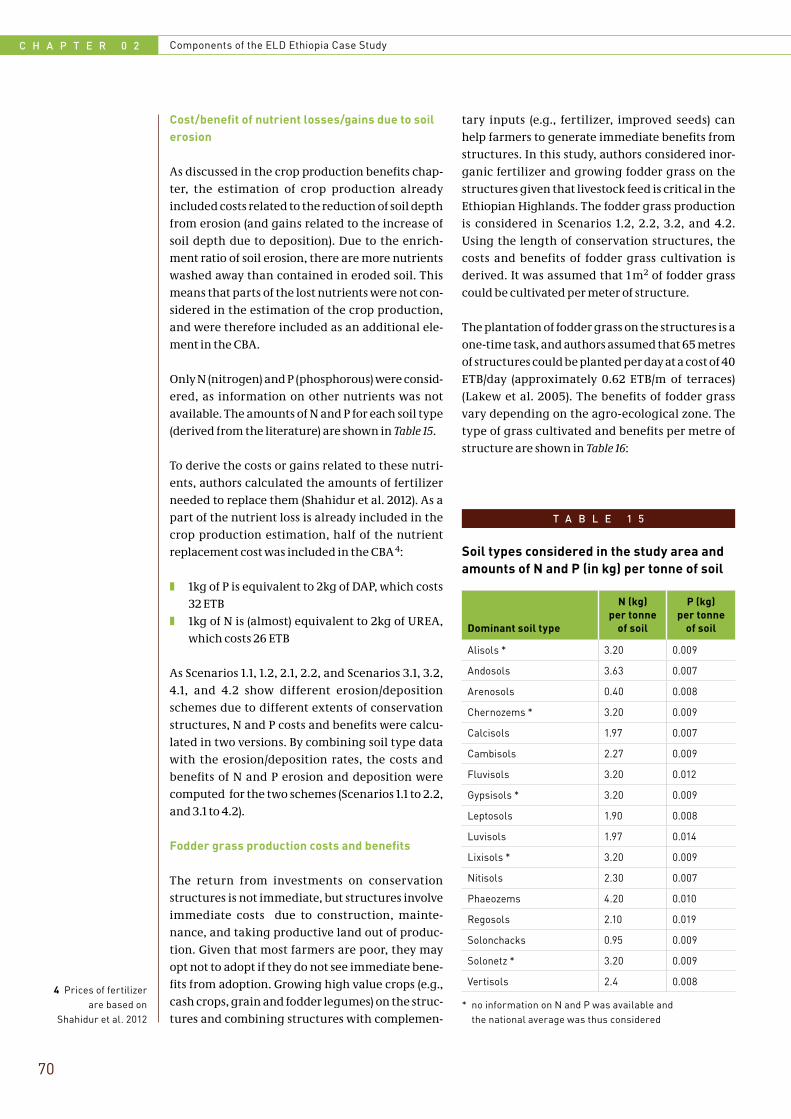
C H A P T E R 0 2 Components of the ELD Ethiopia Case Study
70
Cost/benefit of nutrient losses/gains due to soil erosion
As discussed in the crop production benefits chap-ter, the estimation of crop production already included costs related to the reduction of soil depth from erosion (and gains related to the increase of soil depth due to deposition). Due to the enrich-ment ratio of soil erosion, there are more nutrients washed away than contained in eroded soil. This means that parts of the lost nutrients were not con-sidered in the estimation of the crop production, and were therefore included as an additional ele-ment in the CBA.
Only N (nitrogen) and P (phosphorous) were consid-ered, as information on other nutrients was not available. The amounts of N and P for each soil type (derived from the literature) are shown in Table 15.
To derive the costs or gains related to these nutri-ents, authors calculated the amounts of fertilizer needed to replace them (Shahidur et al. 2012). As a part of the nutrient loss is already included in the crop production estimation, half of the nutrient replacement cost was included in the CBA 4:
❚❚ 1kg of P is equivalent to 2kg of DAP, which costs 32 ETB
❚❚ 1kg of N is (almost) equivalent to 2kg of UREA, which costs 26 ETB
As Scenarios 1.1, 1.2, 2.1, 2.2, and Scenarios 3.1, 3.2, 4.1, and 4.2 show different erosion/deposition schemes due to different extents of conservation structures, N and P costs and benefits were calcu-lated in two versions. By combining soil type data with the erosion/deposition rates, the costs and benefits of N and P erosion and deposition were computed for the two schemes (Scenarios 1.1 to 2.2, and 3.1 to 4.2).
Fodder grass production costs and benefits
The return from investments on conservation structures is not immediate, but structures involve immediate costs due to construction, mainte-nance, and taking productive land out of produc-tion. Given that most farmers are poor, they may opt not to adopt if they do not see immediate bene-fits from adoption. Growing high value crops (e.g., cash crops, grain and fodder legumes) on the struc-tures and combining structures with complemen-
tary inputs (e.g., fertilizer, improved seeds) can help farmers to generate immediate benefits from structures. In this study, authors considered inor-ganic fertilizer and growing fodder grass on the structures given that livestock feed is critical in the Ethiopian Highlands. The fodder grass production is considered in Scenarios 1.2, 2.2, 3.2, and 4.2. Using the length of conservation structures, the costs and benefits of fodder grass cultivation is derived. It was assumed that 1 m2 of fodder grass could be cultivated per meter of structure.
The plantation of fodder grass on the structures is a one-time task, and authors assumed that 65 metres of structures could be planted per day at a cost of 40 ETB/day (approximately 0.62 ETB/m of terraces) (Lakew et al. 2005). The benefits of fodder grass vary depending on the agro-ecological zone. The type of grass cultivated and benefits per metre of structure are shown in Table 16:
T A B L E 1 5
Soil types considered in the study area and amounts of N and P (in kg) per tonne of soil
Dominant soil type
N (kg) per tonne
of soil
P (kg) per tonne
of soil
Alisols * 3.20 0.009
Andosols 3.63 0.007
Arenosols 0.40 0.008
Chernozems * 3.20 0.009
Calcisols 1.97 0.007
Cambisols 2.27 0.009
Fluvisols 3.20 0.012
Gypsisols * 3.20 0.009
Leptosols 1.90 0.008
Luvisols 1.97 0.014
Lixisols * 3.20 0.009
Nitisols 2.30 0.007
Phaeozems 4.20 0.010
Regosols 2.10 0.019
Solonchacks 0.95 0.009
Solonetz * 3.20 0.009
Vertisols 2.4 0.0084 Prices of fertilizer
are based on Shahidur et al. 2012
* no information on N and P was available and the national average was thus considered
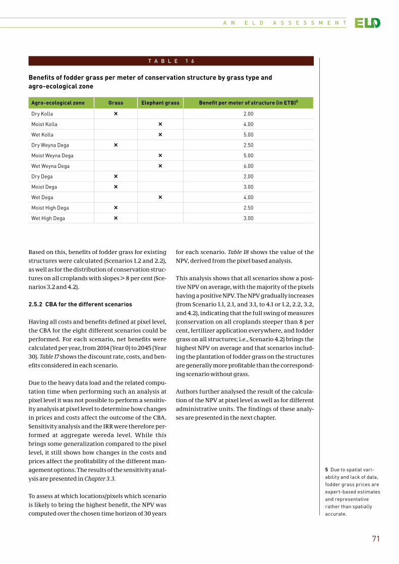
A N E L D A S S E S S M E N T
71
Based on this, benefits of fodder grass for existing structures were calculated (Scenarios 1.2 and 2.2), as well as for the distribution of conservation struc-tures on all croplands with slopes > 8 per cent (Sce-narios 3.2 and 4.2).
2.5.2 CBA for the different scenarios
Having all costs and benefits defined at pixel level, the CBA for the eight different scenarios could be performed. For each scenario, net benefits were calculated per year, from 2014 (Year 0) to 2045 (Year 30). Table 17 shows the discount rate, costs, and ben-efits considered in each scenario.
Due to the heavy data load and the related compu-tation time when performing such an analysis at pixel level it was not possible to perform a sensitiv-ity analysis at pixel level to determine how changes in prices and costs affect the outcome of the CBA. Sensitivity analysis and the IRR were therefore per-formed at aggregate wereda level. While this brings some generalization compared to the pixel level, it still shows how changes in the costs and prices affect the profitability of the different man-agement options. The results of the sensitivity anal-ysis are presented in Chapter 3.3.
To assess at which locations/pixels which scenario is likely to bring the highest benefit, the NPV was computed over the chosen time horizon of 30 years
for each scenario. Table 18 shows the value of the NPV, derived from the pixel based analysis.
This analysis shows that all scenarios show a posi-tive NPV on average, with the majority of the pixels having a positive NPV. The NPV gradually increases (from Scenario 1.1, 2.1, and 3.1, to 4.1 or 1.2, 2.2, 3.2, and 4.2), indicating that the full swing of measures (conservation on all croplands steeper than 8 per cent, fertilizer application everywhere, and fodder grass on all structures; i.e., Scenario 4.2) brings the highest NPV on average and that scenarios includ-ing the plantation of fodder grass on the structures are generally more profitable than the correspond-ing scenario without grass.
Authors further analysed the result of the calcula-tion of the NPV at pixel level as well as for different administrative units. The findings of these analy-ses are presented in the next chapter.
5 Due to spatial vari-ability and lack of data, fodder grass prices are expert-based estimates and representative rather than spatially accurate.
T A B L E 1 6
Benefits of fodder grass per meter of conservation structure by grass type and agro-ecological zone
Agro-ecological zone Grass Elephant grass Benefit per meter of structure (in ETB)5
Dry Kolla l 2.00
Moist Kolla l 4.00
Wet Kolla l 5.00
Dry Weyna Dega l 2.50
Moist Weyna Dega l 5.00
Wet Weyna Dega l 6.00
Dry Dega l 2.00
Moist Dega l 3.00
Wet Dega l 4.00
Moist High Dega l 2.50
Wet High Dega l 3.00
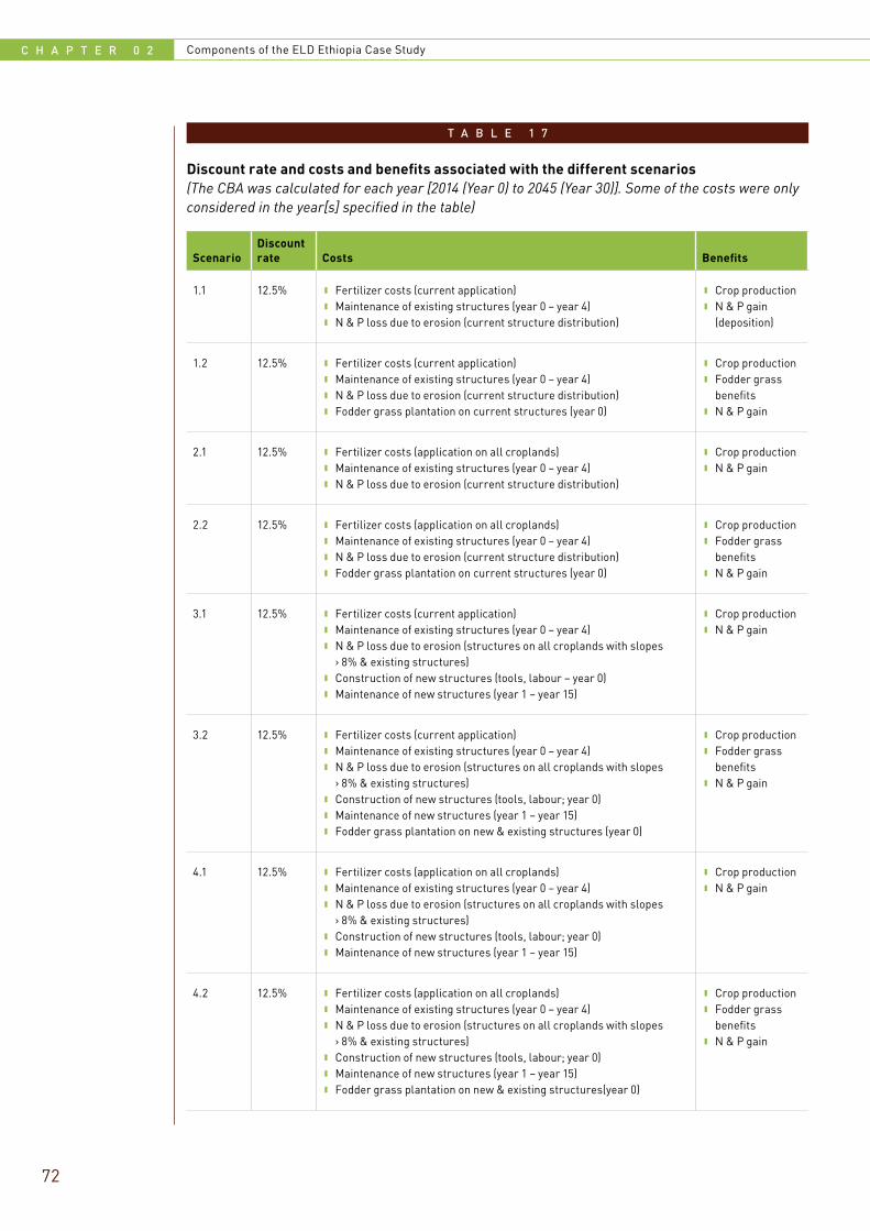
C H A P T E R 0 2 Components of the ELD Ethiopia Case Study
72
T A B L E 1 7
Discount rate and costs and benefits associated with the different scenarios(The CBA was calculated for each year [2014 (Year 0) to 2045 (Year 30)]. Some of the costs were only considered in the year[s] specified in the table)
ScenarioDiscount rate Costs Benefits
1.1 12.5% k Fertilizer costs (current application) k Maintenance of existing structures (year 0 – year 4) k N & P loss due to erosion (current structure distribution)
k Crop production k N & P gain
(deposition)
1.2 12.5% k Fertilizer costs (current application)k Maintenance of existing structures (year 0 – year 4)k N & P loss due to erosion (current structure distribution)k Fodder grass plantation on current structures (year 0)
k Crop productionk Fodder grass
benefitsk N & P gain
2.1 12.5% k Fertilizer costs (application on all croplands)k Maintenance of existing structures (year 0 – year 4)k N & P loss due to erosion (current structure distribution)
k Crop productionk N & P gain
2.2 12.5% k Fertilizer costs (application on all croplands)k Maintenance of existing structures (year 0 – year 4)k N & P loss due to erosion (current structure distribution)k Fodder grass plantation on current structures (year 0)
k Crop productionk Fodder grass
benefits k N & P gain
3.1 12.5% k Fertilizer costs (current application) k Maintenance of existing structures (year 0 – year 4)k N & P loss due to erosion (structures on all croplands with slopes
› 8% & existing structures)k Construction of new structures (tools, labour – year 0)k Maintenance of new structures (year 1 – year 15)
k Crop productionk N & P gain
3.2 12.5% k Fertilizer costs (current application) k Maintenance of existing structures (year 0 – year 4)k N & P loss due to erosion (structures on all croplands with slopes
› 8% & existing structures)k Construction of new structures (tools, labour; year 0)k Maintenance of new structures (year 1 – year 15)k Fodder grass plantation on new & existing structures (year 0)
k Crop productionk Fodder grass
benefitsk N & P gain
4.1 12.5% k Fertilizer costs (application on all croplands)k Maintenance of existing structures (year 0 – year 4)k N & P loss due to erosion (structures on all croplands with slopes
› 8% & existing structures)k Construction of new structures (tools, labour; year 0)k Maintenance of new structures (year 1 – year 15)
k Crop productionk N & P gain
4.2 12.5% k Fertilizer costs (application on all croplands)k Maintenance of existing structures (year 0 – year 4)k N & P loss due to erosion (structures on all croplands with slopes
› 8% & existing structures)k Construction of new structures (tools, labour; year 0)k Maintenance of new structures (year 1 – year 15)k Fodder grass plantation on new & existing structures(year 0)
k Crop productionk Fodder grass
benefitsk N & P gain
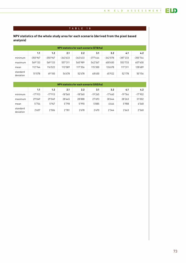
A N E L D A S S E S S M E N T
73
T A B L E 1 8
NPV statistics of the whole study area for each scenario (derived from the pixel based analysis)
NPV statistics for each scenario (ETB/ha)
1.1 1.2 2.1 2.2 3.1 3.2 4.1 4.2
minimum -350'967 -350'967 -363'633 -363'633 -377'444 -342'078 -387'233 -350'744
maximum 569'133 569'133 557'311 565'989 542'567 600'400 553'733 607'400
mean 112'744 116'522 113'589 117'356 115'300 126'678 117'311 128'689
standard deviation
51'078 49'100 54'478 52'478 48'400 45'922 52'178 50'156
NPV statistics for each scenario (USD/ha)
1.1 1.2 2.1 2.2 3.1 3.2 4.1 4.2
minimum -17'913 -17'913 -18'560 -18'560 -19'265 -17'460 -19'764 -17'902
maximum 29'049 29'049 28'445 28'888 27'693 30'644 28'263 31'002
mean 5'754 5'947 5'798 5'990 5'885 6'466 5'988 6'568
standard deviation
2'607 2'506 2'781 2'678 2'470 2'344 2'663 2'560
C H A P T E R
03
74
Synthesis and discussion of livelihood options
3.1 Achievements and limitations
The ELD Ethiopia Case Study concentrated mainly on the productive functions of Ethiopia’s highland ecosystems. The objective was to find out how best to minimize soil degradation and achieve better cropland productivity and longterm sustainability (i.e., reducing on-site impacts). The study further attempted to outline solutions that help to reduce sediment yields in river basins to ensure sustaina-bility of reservoirs for hydropower generation and other purposes such as water supply and small-scale irrigation (i.e., reducing off-site impacts).
The analyses within each of the five components of the case study have resulted in the following spa-tially explicit datasets at a resolution of 30 m x 30 m:
❚❚ Current state and rates of soil degradation – including SLM technologies implemented – as well as resulting crop production and their mon-etary value (enables discussion of the profitabil-ity of currently implemented SLM technologies)
❚❚ Profitability of improving current SWC technol-ogies and of introducing improved SLM tech-nologies in areas where SWC structures have not yet been built
This methodology is rather unique: The authors worked with farmers’ field size area unit (30m pix-els) to perform a spatially explicit economic valuation of SLM technologies. Yet the case study covered a very large area of 600,000 km2 with over 200,000 km2 of croplands. The shortcomings of the data used were mentioned in the descriptions of the case study components in Chapter 2:
❚❚ Lack of spatially explicit data on the distribu-tion of existing conservation structures;
❚❚ Lack of spatially explicit data on the distribu-tion of current fertilizer application;
❚❚ Lack of data on the current sediment yield in any one of the large river basins in Ethiopia;
❚❚ Lack of spatial data for some of the parameters such as the benefits of crop residue use.
Authors had to neglect some parameters or use proxies to produce these layers. This can affect the accuracy of results at the pixel level, whereas results at aggregated levels are more reliable. As soon as more accurate layers become available, this analysis can be run again and thereby improved.
In the scenario analysis, authors did not change the current extent of croplands over the 30 years of sce-nario development, nor were agronomic changes included, such as plant breeding, plant protection, changes in the farming system, expansion of crop-lands or other land use types, deforestation, or cli-mate change. The study quantified the on-site impacts of soil erosion by water related to crop pro-duction; all other on-site impacts and off-site impacts are not addressed. However, if these were included as variables, the model developed could fairly easily be used to develop scenarios of sustain-able agricultural development while maintaining the ecological functions of soil and water. Finally, one might ask whether 30 years is forward-looking enough. Soil erosion is a relatively slow process: over a period of 30 years it will reduce soil depth on cropland by an average of ‘only’ 6 cm. However, knowing that soil degradation is almost irreversi-ble, authors estimate that it may take as much as 100–300 years for the soil to regain those 6 cm (Hurni 1983), and conclude that soil erosion must be reduced to a minimum.
3.2 Pertinent questions at the national level
How important is soil erosion?
The scenario analysis carried out for the ELD Ethio-pia Case Study shows that soil erosion is indeed the most important process of land degradation in the rainfed agricultural areas of Ethiopia. Table 19 pre-sents the net erosion/deposition totals for the most important land cover classes in the study area, as well as on an average per hectare basis. Soil loss is greatest on croplands, which shows how important
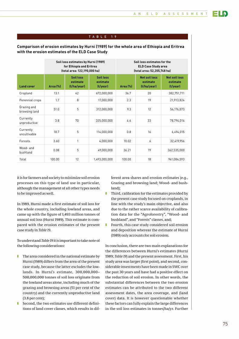
A N E L D A S S E S S M E N T
75
it is for farmers and society to minimize soil erosion processes on this type of land use in particular, although the management of all other types needs to be improved as well.
In 1989, Hurni made a first estimate of soil loss for the whole country, including lowland areas, and came up with the figure of 1,493 million tonnes of annual soil loss (Hurni 1989). This estimate is com-pared with the erosion estimates of the present case study in Table 19.
To understand Table 19 it is important to take note of the following considerations:
❚❚ The area considered in the national estimate by Hurni (1989) differs from the area of the present case study, because the latter excludes the low-lands. In Hurni’s estimate, 300,000,000–500,000,000 tonnes of soil loss originate from the lowland areas alone, including much of the grazing and browsing areas (51 per cent of the country) and the currently unproductive land (3.8 per cent);
❚❚ Second, the two estimates use different defini-tions of land cover classes, which results in dif-
ferent area shares and erosion estimates (e.g., Grazing and browsing land; Wood- and bush-land);
❚❚ Third, calibration for the estimates provided by the present case study focused on croplands, in line with the study’s main objective, and also due to the rather scarce availability of calibra-tion data for the “Agroforestry”, “Wood- and bushland”, and “Forests” classes, and;
❚❚ Fourth, this case study considered soil erosion and deposition whereas the estimate of Hurni (1989) only accounts for soil erosion.
In conclusion, there are two main explanations for the differences between Hurni’s estimates (Hurni 1989; Table 19) and the present assessment. First, his study area was larger (first point), and second, con-siderable investments have been made in SWC over the past 30 years and have had a positive effect on the reduction of soil erosion. In other words, the substantial differences between the two erosion estimates can be attributed to the two different assessment dates, the area coverage, and (land cover) data. It is however questionable whether these factors can fully explain the large differences in the soil loss estimates in tonnes/ha/yr. Further
Soil loss estimates by Hurni (1989) for Ethiopia and Eritrea
(total area: 122,190,000 ha)
Soil loss estimates for the ELD Case Study area
(total area: 52,205,748 ha)
Land cover Area (%)
Soil loss estimate
(t/ha/year)
Soil loss estimate (t/year) Area (%)
Net soil loss estimate
(t/ha/year)
Net soil loss estimate (t/year)
Cropland 13.1 42 672,000,000 36.7 20 382,751,711
Perennial crops 1.7 8 17,000,000 2.3 19 21,913,824
Grazing and browsing land
51.0 5 312,000,000 9.3 12 56,176,073
Currently unproductive
3.8 70 325,000,000 4.6 33 78,794,014
Currently uncultivable
18.7 5 114,000,000 0.8 16 6,494,015
Forests 3.60 1 4,000,000 10.02 6 32,419,956
Wood- and bushland
0.08 5 49,000,000 36.21 19 362,535,000
Total 100.00 12 1,493,000,000 100.00 18 941,084,593
T A B L E 1 9
Comparison of erosion estimates by Hurni (1989) for the whole area of Ethiopia and Eritrea with the erosion estimates of the ELD Case Study
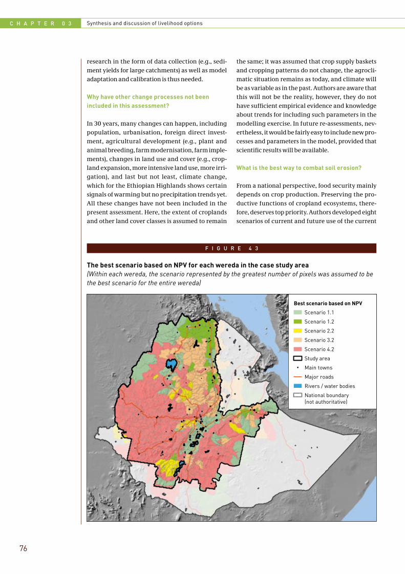
C H A P T E R 0 3 Synthesis and discussion of livelihood options
76
research in the form of data collection (e.g., sedi-ment yields for large catchments) as well as model adaptation and calibration is thus needed.
Why have other change processes not been included in this assessment?
In 30 years, many changes can happen, including population, urbanisation, foreign direct invest-ment, agricultural development (e.g., plant and animal breeding, farm modernisation, farm imple-ments), changes in land use and cover (e.g., crop-land expansion, more intensive land use, more irri-gation), and last but not least, climate change, which for the Ethiopian Highlands shows certain signals of warming but no precipitation trends yet. All these changes have not been included in the present assessment. Here, the extent of croplands and other land cover classes is assumed to remain
the same; it was assumed that crop supply baskets and cropping patterns do not change, the agrocli-matic situation remains as today, and climate will be as variable as in the past. Authors are aware that this will not be the reality, however, they do not have sufficient empirical evidence and knowledge about trends for including such parameters in the modelling exercise. In future re-assessments, nev-ertheless, it would be fairly easy to include new pro-cesses and parameters in the model, provided that scientific results will be available.
What is the best way to combat soil erosion?
From a national perspective, food security mainly depends on crop production. Preserving the pro-ductive functions of cropland ecosystems, there-fore, deserves top priority. Authors developed eight scenarios of current and future use of the current
F I G U R E 4 3
The best scenario based on NPV for each wereda in the case study area(Within each wereda, the scenario represented by the greatest number of pixels was assumed to be the best scenario for the entire wereda)
!
Scenario 1.1
Scenario 1.2
Scenario 2.2
Scenario 3.2
Scenario 4.2
Study area
Main towns
Major roads
Rivers / water bodies
National boundary(not authoritative)
Best scenario based on NPV
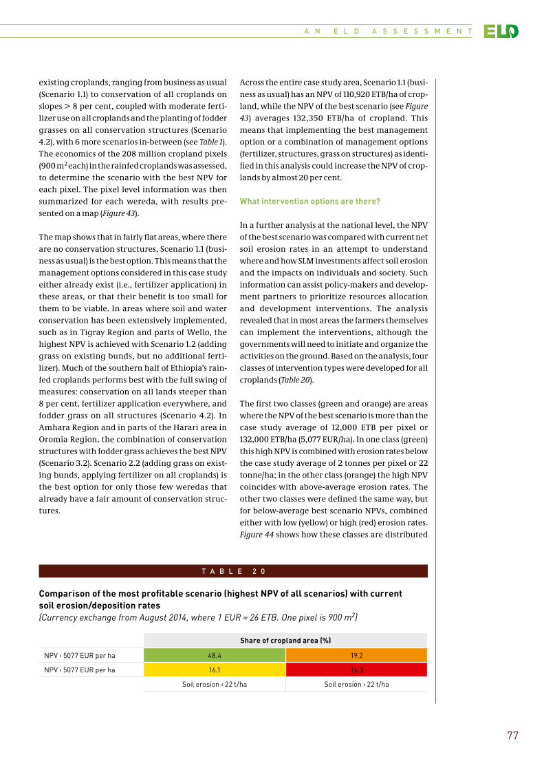
A N E L D A S S E S S M E N T
77
existing croplands, ranging from business as usual (Scenario 1.1) to conservation of all croplands on slopes > 8 per cent, coupled with moderate ferti-lizer use on all croplands and the planting of fodder grasses on all conservation structures (Scenario 4.2), with 6 more scenarios in-between (see Table 1). The economics of the 208 million cropland pixels (900 m2 each) in the rainfed croplands was assessed, to determine the scenario with the best NPV for each pixel. The pixel level information was then summarized for each wereda, with results pre-sented on a map (Figure 43).
The map shows that in fairly flat areas, where there are no conservation structures, Scenario 1.1 (busi-ness as usual) is the best option. This means that the management options considered in this case study either already exist (i.e., fertilizer application) in these areas, or that their benefit is too small for them to be viable. In areas where soil and water conservation has been extensively implemented, such as in Tigray Region and parts of Wello, the highest NPV is achieved with Scenario 1.2 (adding grass on existing bunds, but no additional ferti-lizer). Much of the southern half of Ethiopia’s rain-fed croplands performs best with the full swing of measures: conservation on all lands steeper than 8 per cent, fertilizer application everywhere, and fodder grass on all structures (Scenario 4.2). In Amhara Region and in parts of the Harari area in Oromia Region, the combination of conservation structures with fodder grass achieves the best NPV (Scenario 3.2). Scenario 2.2 (adding grass on exist-ing bunds, applying fertilizer on all croplands) is the best option for only those few weredas that already have a fair amount of conservation struc-tures.
Across the entire case study area, Scenario 1.1 (busi-ness as usual) has an NPV of 110,920 ETB/ha of crop-land, while the NPV of the best scenario (see Figure 43) averages 132,350 ETB/ha of cropland. This means that implementing the best management option or a combination of management options (fertilizer, structures, grass on structures) as identi-fied in this analysis could increase the NPV of crop-lands by almost 20 per cent.
What intervention options are there?
In a further analysis at the national level, the NPV of the best scenario was compared with current net soil erosion rates in an attempt to understand where and how SLM investments affect soil erosion and the impacts on individuals and society. Such information can assist policy-makers and develop-ment partners to prioritize resources allocation and development interventions. The analysis revealed that in most areas the farmers themselves can implement the interventions, although the governments will need to initiate and organize the activities on the ground. Based on the analysis, four classes of intervention types were developed for all croplands (Table 20).
The first two classes (green and orange) are areas where the NPV of the best scenario is more than the case study average of 12,000 ETB per pixel or 132,000 ETB/ha (5,077 EUR/ha). In one class (green) this high NPV is combined with erosion rates below the case study average of 2 tonnes per pixel or 22 tonne/ha; in the other class (orange) the high NPV coincides with above-average erosion rates. The other two classes were defined the same way, but for below-average best scenario NPVs, combined either with low (yellow) or high (red) erosion rates. Figure 44 shows how these classes are distributed
T A B L E 2 0
Comparison of the most profitable scenario (highest NPV of all scenarios) with current soil erosion/deposition rates(Currency exchange from August 2014, where 1 EUR = 26 ETB. One pixel is 900 m2)
Share of cropland area (%)
NPV › 5077 EUR per ha 48.4 19.2
NPV ‹ 5077 EUR per ha 16.1 16.3
Soil erosion ‹ 22 t/ha Soil erosion › 22 t/ha
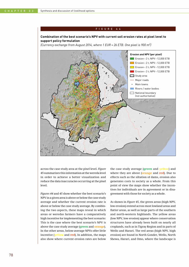
C H A P T E R 0 3 Synthesis and discussion of livelihood options
78
across the case study area at the pixel level. Figure 45 summarizes this information at the wereda level in order to achieve a better visualization and reduce the data inaccuracies occurring at the pixel level.
Figures 44 and 45 show whether the best scenario’s NPV in a given area is above or below the case study average and whether the current erosion rate is above or below the case study average. By combin-ing the two aspects, these maps reveal in which areas or weredas farmers have a comparatively high incentive for implementing the best scenario: This is the case where the best scenario’s NPV is above the case study average (green and orange). In the other areas, below-average NPVs offer little incentive (yellow and red). In addition, the maps also show where current erosion rates are below
the case study average (green and yellow) and where they are above (orange and red). Due to effects such as the siltation of dams, erosion also generates costs to society as a whole. From this point of view the maps show whether the incen-tives for individuals are in agreement or in disa-greement with those for society as a whole.
As shown in Figure 45, the green areas (high NPV, low erosion) extend across most lowland areas and flatter areas, as well as large parts of the southern and north-western highlands. The yellow areas (low NPV, low erosion) appear where conservation structures have already been built on nearly all croplands, such as in Tigray Region and in parts of Wello and Harari. The red areas (high NPV, high erosion) are found in North Gonder, Wello, North Shewa, Harari, and Omo, where the landscape is
F I G U R E 4 4
Combination of the best scenario’s NPV with current soil erosion rates at pixel level to support policy formulation(Currency exchange from August 2014, where 1 EUR = 26 ETB. One pixel is 900 m2)
!
Erosion ‹ 2 t; NPV › 12,000 ETB
Erosion › 2 t; NPV › 12,000 ETB
Erosion ‹ 2 t; NPV ‹ 12,000 ETB
Erosion › 2 t; NPV ‹ 12,000 ETB
Study area
Major roads
Main towns
Rivers / water bodies
National boundary(not authoritative)
Erosion and NPV (per pixel)
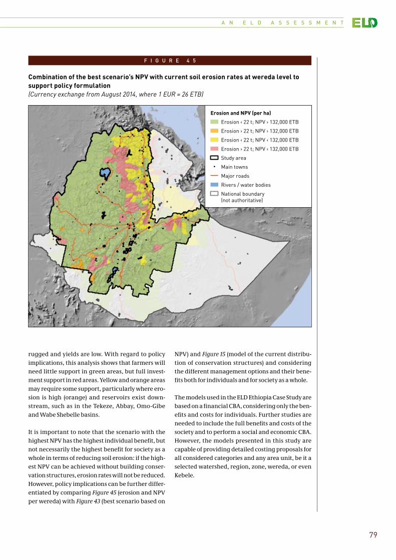
A N E L D A S S E S S M E N T
79
rugged and yields are low. With regard to policy implications, this analysis shows that farmers will need little support in green areas, but full invest-ment support in red areas. Yellow and orange areas may require some support, particularly where ero-sion is high (orange) and reservoirs exist down-stream, such as in the Tekeze, Abbay, Omo-Gibe and Wabe Shebelle basins.
It is important to note that the scenario with the highest NPV has the highest individual benefit, but not necessarily the highest benefit for society as a whole in terms of reducing soil erosion: if the high-est NPV can be achieved without building conser-vation structures, erosion rates will not be reduced. However, policy implications can be further differ-entiated by comparing Figure 45 (erosion and NPV per wereda) with Figure 43 (best scenario based on
NPV) and Figure 15 (model of the current distribu-tion of conservation structures) and considering the different management options and their bene-fits both for individuals and for society as a whole. The models used in the ELD Ethiopia Case Study are based on a financial CBA, considering only the ben-efits and costs for individuals. Further studies are needed to include the full benefits and costs of the society and to perform a social and economic CBA. However, the models presented in this study are capable of providing detailed costing proposals for all considered categories and any area unit, be it a selected watershed, region, zone, wereda, or even Kebele.
F I G U R E 4 5
Combination of the best scenario’s NPV with current soil erosion rates at wereda level to support policy formulation(Currency exchange from August 2014, where 1 EUR = 26 ETB)
!
Erosion ‹ 22 t; NPV › 132,000 ETB
Erosion › 22 t; NPV › 132,000 ETB
Erosion ‹ 22 t; NPV ‹ 132,000 ETB
Erosion › 22 t; NPV ‹ 132,000 ETB
Study area
Main towns
Major roads
Rivers / water bodies
National boundary(not authoritative)
Erosion and NPV (per ha)
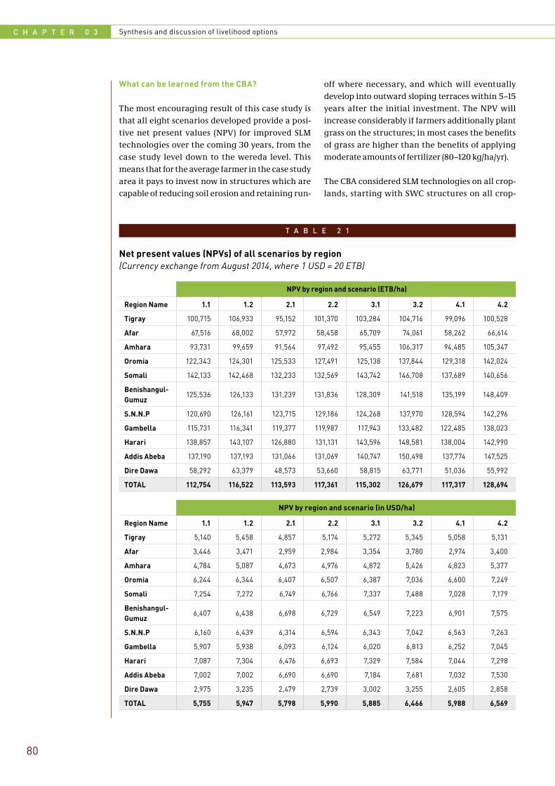
C H A P T E R 0 3 Synthesis and discussion of livelihood options
80
What can be learned from the CBA?
The most encouraging result of this case study is that all eight scenarios developed provide a posi-tive net present values (NPV) for improved SLM technologies over the coming 30 years, from the case study level down to the wereda level. This means that for the average farmer in the case study area it pays to invest now in structures which are capable of reducing soil erosion and retaining run-
off where necessary, and which will eventually develop into outward sloping terraces within 5–15 years after the initial investment. The NPV will increase considerably if farmers additionally plant grass on the structures; in most cases the benefits of grass are higher than the benefits of applying moderate amounts of fertilizer (80–120 kg/ha/yr).
The CBA considered SLM technologies on all crop-lands, starting with SWC structures on all crop-
T A B L E 2 1
Net present values (NPVs) of all scenarios by region(Currency exchange from August 2014, where 1 USD = 20 ETB)
NPV by region and scenario (ETB/ha)
Region Name 1.1 1.2 2.1 2.2 3.1 3.2 4.1 4.2
Tigray 100,715 106,933 95,152 101,370 103,284 104,716 99,096 100,528
Afar 67,516 68,002 57,972 58,458 65,709 74,061 58,262 66,614
Amhara 93,731 99,659 91,564 97,492 95,455 106,317 94,485 105,347
Oromia 122,343 124,301 125,533 127,491 125,138 137,844 129,318 142,024
Somali 142,133 142,468 132,233 132,569 143,742 146,708 137,689 140,656
Benishangul-Gumuz
125,536 126,133 131,239 131,836 128,309 141,518 135,199 148,409
S.N.N.P 120,690 126,161 123,715 129,186 124,268 137,970 128,594 142,296
Gambella 115,731 116,341 119,377 119,987 117,943 133,482 122,485 138,023
Harari 138,857 143,107 126,880 131,131 143,596 148,581 138,004 142,990
Addis Abeba 137,190 137,193 131,066 131,069 140,747 150,498 137,774 147,525
Dire Dawa 58,292 63,379 48,573 53,660 58,815 63,771 51,036 55,992
TOTAL 112,754 116,522 113,593 117,361 115,302 126,679 117,317 128,694
NPV by region and scenario (in USD/ha)
Region Name 1.1 1.2 2.1 2.2 3.1 3.2 4.1 4.2
Tigray 5,140 5,458 4,857 5,174 5,272 5,345 5,058 5,131
Afar 3,446 3,471 2,959 2,984 3,354 3,780 2,974 3,400
Amhara 4,784 5,087 4,673 4,976 4,872 5,426 4,823 5,377
Oromia 6,244 6,344 6,407 6,507 6,387 7,036 6,600 7,249
Somali 7,254 7,272 6,749 6,766 7,337 7,488 7,028 7,179
Benishangul-Gumuz
6,407 6,438 6,698 6,729 6,549 7,223 6,901 7,575
S.N.N.P 6,160 6,439 6,314 6,594 6,343 7,042 6,563 7,263
Gambella 5,907 5,938 6,093 6,124 6,020 6,813 6,252 7,045
Harari 7,087 7,304 6,476 6,693 7,329 7,584 7,044 7,298
Addis Abeba 7,002 7,002 6,690 6,690 7,184 7,681 7,032 7,530
Dire Dawa 2,975 3,235 2,479 2,739 3,002 3,255 2,605 2,858
TOTAL 5,755 5,947 5,798 5,990 5,885 6,466 5,988 6,569
A N E L D A S S E S S M E N T
81
lands steeper than 8 per cent and adding moderate application of fertilizer and, importantly, grass planting on all structures. If all three measures are implemented – which does not necessarily achieve the highest NPVs – crop production will increase by nearly 10 per cent in 30 years; the management option with the highest NPV – which does not nec-essarily include all measures – still achieves an average increase by 7 per cent in 30 years. Table 21 shows NPVs of all scenarios by region, in ETB/ha.
In the view of the authors, the eight scenarios pre-sented above are a modest, but realistic vision. This vision does not include the benefits of potential agricultural developments such as new crop varie-ties, maximum fertilizer application, and best agri-cultural management. Due to the omission of such additional management practices it is likely that the benefits have been underestimated. These sce-narios focus above all on achieving sustainable ecosystem functions with regard to soil and water in the long-term. The least promising scenario is business as usual. Although SWC has already been implemented on an assumed 18 per cent of crop-lands over the past four decades, this study con-cludes that all sloping croplands need to be treated. This concerns 77 per cent of Ethiopia’s croplands, as only 23 per cent of croplands are on slopes smaller than 8 per cent.
What are the total investment costs for the case study area?
Authors also wanted to know what investment is needed to initiate SWC on these remaining sloping croplands as a basis for subsequent SLM improve-ments. Costs were calculated based on the 50 per cent of the croplands where structures still need to be built (more than 10 million hectares), and arrived at a total cost of 44 billion ETB, or 1.7 billion EUR in August 2014 to cover labour and tools, not including maintenance costs. This amount would have to be invested at the beginning of the 30 year period, either by the government (in areas with high erosion and low NVP) or by the farmers them-selves (most areas). The split between costs to the government and in kind costs to farmers according to Table 20 (above) can be calculated using the ELD Ethiopia Case Study database at the Water and Land Resource Centre (WLRC).
Can sediments in the rivers and hence siltation of reservoirs be reduced?
According to the erosion/deposition modelling, the study area has a net loss of about 941 million tonnes of soil sediments/yr. A look at where these sediments originate from reveals the alarming fact that over 50 per cent of all land in the case study area is affected by a net loss of soil. This soil leaves the case study area as suspended sediment in riv-ers, or is deposited in the inland lakes and smaller wetlands beforehand. The other half of the case study area nevertheless has a positive balance due to sediment accumulation from upslope, meaning that soil lost upslope is deposited downslope before it reaches a river and is carried away as suspended sediment. It would be tempting to conclude that conserving all degrading rainfed cropland would reduce sediment yields in the rivers. This hypothe-sis is in fact supported by the long-term monitoring observatories of the SCRP, where sediment yields were reduced to about one third of the amounts measured one to two years before conservation structures were built. These catchments, however, are small compared to Ethiopia’s larger water-sheds, and it is unknown how clearer water run-ning down from conserved lands would perform in terms of eroding river banks. In conclusion, authors refrain from predicting that SLM measures will reduce suspended sediment concentrations in large rivers, although there are strong arguments in support of this hypothesis.
By how much can soil erosion from cropland be reduced?
Looking exclusively at cropland, about 60 per cent of all cropland in the case study area is affected by net erosion, resulting in about 380 million tonnes of sediments per year, or 20 tonnes per ha of crop-land per year. Loss of these sediments also entails a huge loss of nutrients (N and P). Assuming that these nutrients need to be replaced by fertilizer to maintain productivity, the cost of nutrient loss alone amounts to 14.4 billion ETB/yr. If all croplands steeper than 8 per cent were conserved, the amount of sediments could be reduced to 222 million tonnes, or 12 tonnes/ha/yr on average, an amount that is very nearly tolerable. This reduction in ero-sion would also reduce the cost of nutrient loss by 4.55 billion ETB every year.
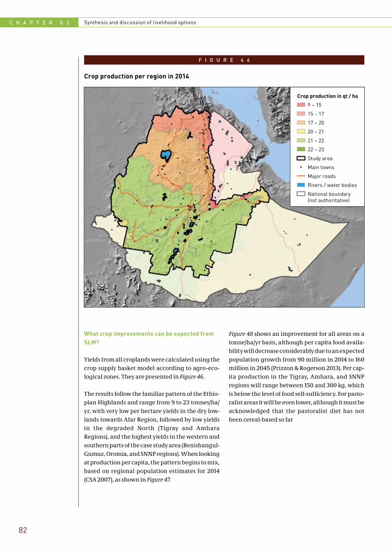
C H A P T E R 0 3 Synthesis and discussion of livelihood options
82
What crop improvements can be expected from SLM?
Yields from all croplands were calculated using the crop supply basket model according to agro-eco-logical zones. They are presented in Figure 46.
The results follow the familiar pattern of the Ethio-pian Highlands and range from 9 to 23 tonnes/ha/yr, with very low per hectare yields in the dry low-lands towards Afar Region, followed by low yields in the degraded North (Tigray and Amhara Regions), and the highest yields in the western and southern parts of the case study area (Benishangul-Gumuz, Oromia, and SNNP regions). When looking at production per capita, the pattern begins to mix, based on regional population estimates for 2014 (CSA 2007), as shown in Figure 47.
Figure 48 shows an improvement for all areas on a tonne/ha/yr basis, although per capita food availa-bility will decrease considerably due to an expected population growth from 90 million in 2014 to 160 million in 2045 (Prizzon & Rogerson 2013). Per cap-ita production in the Tigray, Amhara, and SNNP regions will range between 150 and 300 kg, which is below the level of food self-sufficiency. For pasto-ralist areas it will be even lower, although it must be acknowledged that the pastoralist diet has not been cereal-based so far
F I G U R E 4 6
Crop production per region in 2014
!
9 – 15
15 – 17
17 – 20
20 – 21
21 – 22
22 – 23
Study area
Main towns
Major roads
Rivers / water bodies
National boundary(not authoritative)
Crop production in qt / ha
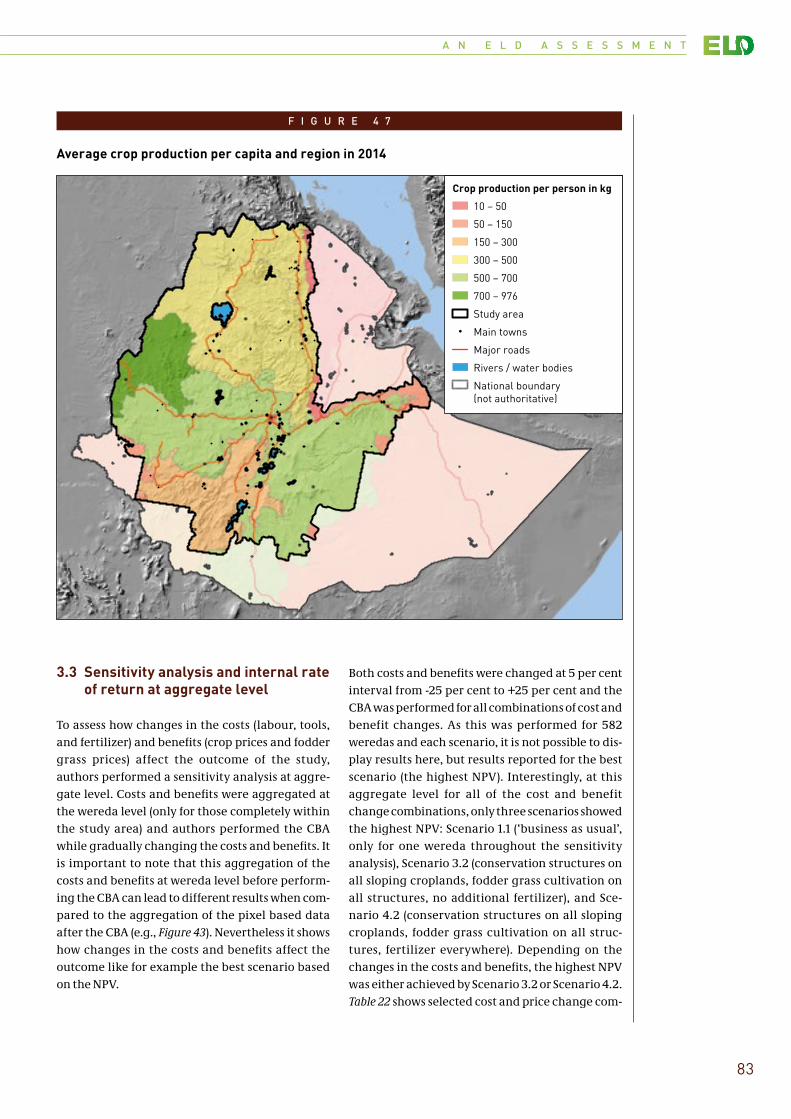
A N E L D A S S E S S M E N T
83
3.3 Sensitivity analysis and internal rate of return at aggregate level
To assess how changes in the costs (labour, tools, and fertilizer) and benefits (crop prices and fodder grass prices) affect the outcome of the study, authors performed a sensitivity analysis at aggre-gate level. Costs and benefits were aggregated at the wereda level (only for those completely within the study area) and authors performed the CBA while gradually changing the costs and benefits. It is important to note that this aggregation of the costs and benefits at wereda level before perform-ing the CBA can lead to different results when com-pared to the aggregation of the pixel based data after the CBA (e.g., Figure 43). Nevertheless it shows how changes in the costs and benefits affect the outcome like for example the best scenario based on the NPV.
Both costs and benefits were changed at 5 per cent interval from -25 per cent to +25 per cent and the CBA was performed for all combinations of cost and benefit changes. As this was performed for 582 weredas and each scenario, it is not possible to dis-play results here, but results reported for the best scenario (the highest NPV). Interestingly, at this aggregate level for all of the cost and benefit change combinations, only three scenarios showed the highest NPV: Scenario 1.1 (‘business as usual’, only for one wereda throughout the sensitivity analysis), Scenario 3.2 (conservation structures on all sloping croplands, fodder grass cultivation on all structures, no additional fertilizer), and Sce-nario 4.2 (conservation structures on all sloping croplands, fodder grass cultivation on all struc-tures, fertilizer everywhere). Depending on the changes in the costs and benefits, the highest NPV was either achieved by Scenario 3.2 or Scenario 4.2. Table 22 shows selected cost and price change com-
F I G U R E 4 7
Average crop production per capita and region in 2014
!
10 – 50
50 – 150
150 – 300
300 – 500
500 – 700
700 – 976
Study area
Main towns
Major roads
Rivers / water bodies
National boundary(not authoritative)
Crop production per person in kg
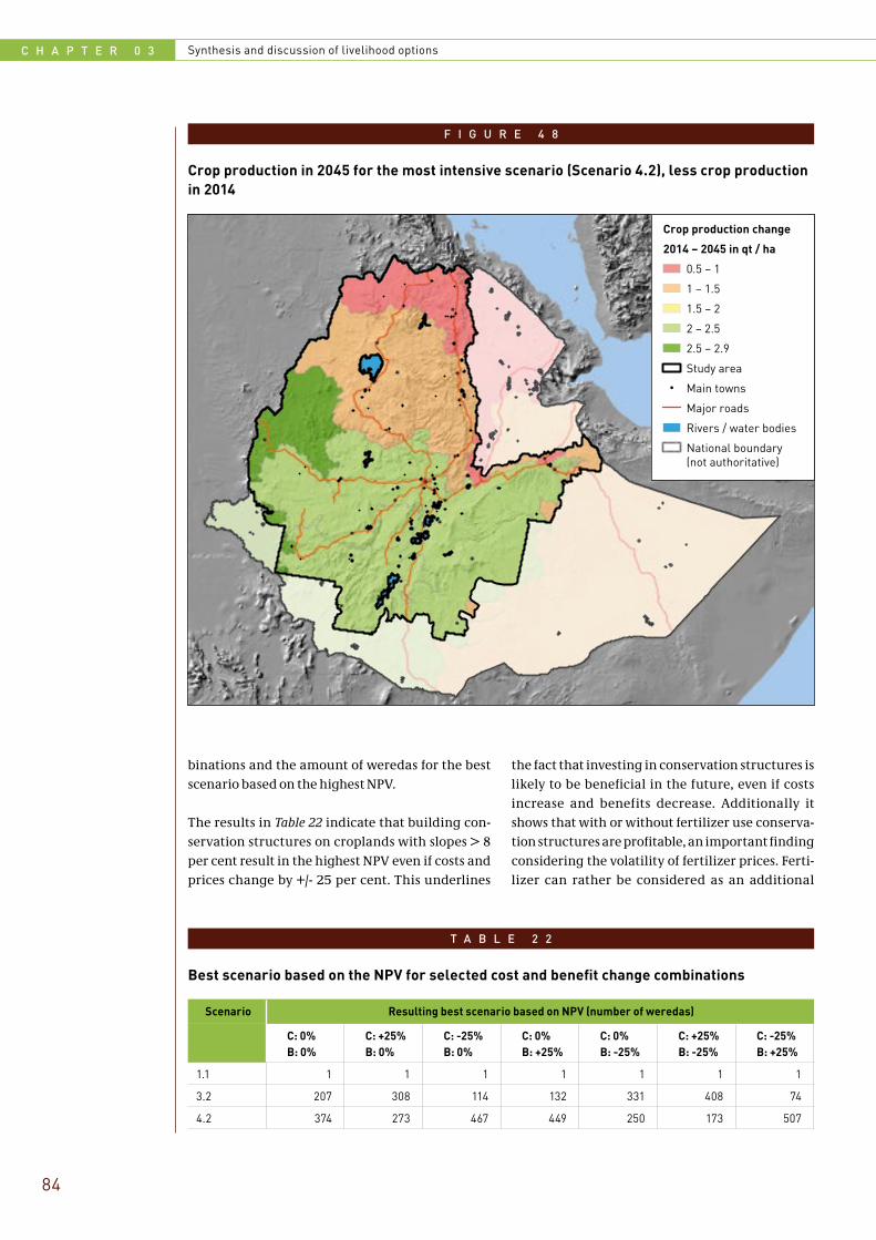
C H A P T E R 0 3 Synthesis and discussion of livelihood options
84
F I G U R E 4 8
Crop production in 2045 for the most intensive scenario (Scenario 4.2), less crop production in 2014
!
0.5 – 1
1 – 1.5
1.5 – 2
2 – 2.5
2.5 – 2.9
Study area
Main towns
Major roads
Rivers / water bodies
National boundary(not authoritative)
Crop production change
2014 – 2045 in qt / ha
binations and the amount of weredas for the best scenario based on the highest NPV.
The results in Table 22 indicate that building con-servation structures on croplands with slopes > 8 per cent result in the highest NPV even if costs and prices change by +/- 25 per cent. This underlines
the fact that investing in conservation structures is likely to be beneficial in the future, even if costs increase and benefits decrease. Additionally it shows that with or without fertilizer use conserva-tion structures are profitable, an important finding considering the volatility of fertilizer prices. Ferti-lizer can rather be considered as an additional
T A B L E 2 2
Best scenario based on the NPV for selected cost and benefit change combinations
Scenario Resulting best scenario based on NPV (number of weredas)
C: 0% B: 0%
C: +25% B: 0%
C: -25% B: 0%
C: 0% B: +25%
C: 0% B: -25%
C: +25% B: -25%
C: -25% B: +25%
1.1 1 1 1 1 1 1 1
3.2 207 308 114 132 331 408 74
4.2 374 273 467 449 250 173 507
A N E L D A S S E S S M E N T
85
measure to increase income, as it is a recurring yearly investment: Depending on the costs, farm-ers can choose whether it is worth to buy fertilizer to increase crop yields and thus income, or to culti-vate the land without fertilizer, on an annual basis.
In addition to the NPV, the IRR was also calculated for each scenario at aggregate wereda level. The IRR was positive (> 50 per cent) for all weredas and scenarios, and 480 of the 582 weredas showed the highest IRR for Scenario 1.1. This means that the ‘business as usual’ scenario with few investments (maintenance of existing structures and using fer-tilizer as currently applied) provides the highest IRR. However, for a subsistence farmer, Scenario 1.1 may not be the most favourable - achieving higher net benefits is likely to be more important than the highest possible IRR. As a result the scenario with the highest NPV is preferable over the scenario with the highest IRR.
This analysis at aggregate level also underlines the importance of spatially explicit, pixel based analy-ses: Comparing the results in Table 22 with Figure 43 shows that some scenarios only became visible’ at pixel level. Through the aggregation of costs and benefits at wereda level before performing the CBA, information was lost (Scenarios 1.1, 1.2, and 2.2), which needs to be kept in mind when inter-preting the results from the sensitivity analysis.
3.4 Alternative livelihood options
It is beyond doubt that a further doubling of Ethio-pia’s rural population in the coming 35–45 years cannot be accommodated with the current crop-land area unless productivity per hectare is sub-stantially increased. Moreover, natural resources will have to be utilized sustainably. Nevertheless, the current growth rates of the Ethiopian economy indicate that the urban centres will continue to grow dramatically in size and number. While 15 per cent of the population (13.5 million) are living in towns in 2014, this share may increase to 40 per cent (about 60–70 million) by 2045. Alternative live-lihoods will develop along the agricultural market chains and outside of them, while small-scale farm-ing might remain the backbone of Ethiopia’s rural economy – with similar farm sizes but higher pro-ductivity and crop diversity, and on much safer ground due to SLM.
In addition, increasing amounts of land might be developed in the western lowlands, which have so far been unsafe for subsistence farming due to dis-eases such as malaria, tsetse, yellow fever, and sleeping sickness. Modern and mechanized farm-ing, coupled with some health infrastructure, is currently advancing into these areas (see land cover map, Figure 4), and seasonal labour migration from the highlands to lowland areas has become a considerable market for hundreds of thousands of labourers every year.
Food security for Ethiopia as a whole will remain an important issue, as the per capita production is likely to decrease over the next three decades. Importing food to meet the needs would mean a step away from food self-sufficiency. An alternative might be for the mechanized production systems outside small-scale farming to produce more for local markets.
3.5 Policy messages for national and regional levels
The ELD Ethiopia Case Study concludes with six major policy messages that are currently being dis-cussed at the national and regional levels, particu-larly in regions where soil and water conservation and sustainable land management have already been included in policies and programmes.
Policy message 1: About one third of today’s rain-fed cropland in Ethiopia does not require immedi-ate action against soil erosion. The other two thirds require conservation structures, in particular all cropland on slopes > 8 per cent. Considerable efforts were made over the past 40 years, and con-servation structures are now present on approxi-mately 18 per cent of all cropland. More than 50 per cent of all cropland still needs to be conserved, as 77 per cent of the cropland shows a slope >8 per cent.
Policy message 2: All scenarios included in this report show that the net present value of soil and water conservation measures and their coupled sustainable land management measures is positive at the wereda and higher levels over a 30 year period and at a discount rate of 12.5 per cent. This means they are worth investing in now. However, the assessment hides extreme cases (i.e., small
C H A P T E R 0 3 Synthesis and discussion of livelihood options
86
areas or individual pixels) where conservation or sustainable land management cannot be profita-ble.
Policy message 3: A total of 44 billion Ethiopian Birr (2014) still needs to be invested in soil and water conservation structures in order to conserve all sloping croplands. Half of the cropland can be con-served by the farmers themselves, i.e., without pay-ment for their work; the other half will require sup-port at various levels because the net present value for the farmers may be low, sedimentation of rivers may be high, or both. It is important to make this investment in the next few years before net erosion has reduced crop production too much.
Policy message 4: Nearly 1 billion tonnes of sus-pended sediments originating from human-induced soil erosion still reach the rivers every year. They silt important reservoirs established for hydropower generation and other purposes, diminishing their functionality. Soil and water conservation is hence also a measure to prolong the life spans of dams and their intended functions.
Policy message 5: There are marked regional dif-ferences regarding which scenario is most appro-priate. In the Tigray Region, it is best to invest in fodder production along bunds (as much of the croplands are conserved), whereas this would first require extensive soil and water conservation in Amhara Region. In the Oromia Region, the full package of conservation, fodder, and fertilizer is most appropriate. However, these priorities need to be spatially differentiated, which can be done using the ELD Ethiopia Case Study database at the WLRC in Addis Abeba.
Policy message 6: This study did not consider the benefits and costs to society in the cost-benefit analysis (e.g., off-site impacts of soil erosion). Other measures like agronomic changes (e.g., improved crop varieties, plant protection, changes in the farming system, compost application, timely weed-ing, mulching, expansion of cropland, or other land use types) were also not considered. Through the omission of these additional parameters, it is likely that the benefits were underestimated. Fur-ther studies are required to assess the effects of these parameters.
3.6 Conclusion
The data analysed or generated for the present ELD Ethiopia Case Study enabled the detection and characterization of spatial patterns related to LULC, soil degradation, and SLM technologies, as well as the definition of areas with similar clusters of potentials and constraints for SWC and SLM. This was done at a high resolution and covered an impressive area that included most of Ethiopia’s rainfed cropland areas. Authors made a new assess-ment of the extent and magnitude of soil erosion, which also included soil deposition rates downslope and resulting net loss in all rivers originating in the highlands. Recommendations are provided regarding the best scenario for each specific loca-tion for the next 30 years, based on economic value. It was not unexpected but certainly satisfying that all scenarios had a positive NPV when compared to business as usual; this means that doing more against soil erosion is better than leaving things the way they are. Recommendation was also given on the amount of investment required to conserve the remaining sloping cultivated lands. The study estimated that a total of 44 billion ETB is required for this task and also shows where direct invest-ment is required and where SWC can be done by farmers themselves.
In conclusion, it should be possible to maintain the current rural population’s livelihoods in most areas, but areas are now identified where this will no longer be possible because the resource base cannot be maintained despite even the best inter-ventions. Within agriculture, options can be devel-oped based on the spatial patterns revealed in this study; existing local case studies, expert knowl-edge, and emerging innovations should also be taken into account. Alternative livelihoods will have to be developed for populations in areas where agriculture is no longer possible, as well as for all rural children that are now growing out of agriculture, and may also no longer have enough land to till. New agricultural areas are being cleared to help maintain food security at the national level, but most people abandoning agri-culture will have to find new livelihoods in grow-ing urban and rural centres. Young rural people already tend to migrate to these environments, and this dynamic is likely to increase in the future. The potential impacts of population growth and migra-tion on rural and urban areas and related liveli-hood options (within and outside of agriculture)
A N E L D A S S E S S M E N T
87
need to be considered. Discussion of such options can build on the data and knowledge base, local case studies, and expert knowledge. Additional spatial data such as accessibility – expressed as travel time to larger towns or markets that provide employment – or proximity to locations with a potential for ecotourism should be included as well, however, the availability and applicability of such data still needs to be determined.
In this respect, the framework established in this study enables the financial valuation of land degra-dation (mainly erosion by water) and different management options and has the potential to be used beyond the current focus on the highland eco-system’s productive function. To date, authors have considered three different management options – conservation structures, fertilizer, and fodder grass – and have shown the potential that such a database has to support informed decision-making and policy formulation. As it is working at the pixel level, the framework is flexible. It can be applied to any given area, and can be updated whenever more accurate data become available. Furthermore, it can be adapted to include more information such as other management options, but also informa-tion not related to agriculture. Including these will enable a more holistic assessment of livelihood options in and outside of agriculture. The work per-formed for the ELD Ethiopia Case Study can there-fore be considered as a step towards the ELD Initia-tive’s goal of providing tools for the total economic valuation of land degradation and sustainable land management.
R E F E R E N C E S
88
References
Abdelsalam, A . (assisted by Ismail, U.H.E .) (2008).
Sediment in the Nile River System. International
Hyd r olo g ic a l P r o g ra m me a nd I nter n at ion a l
Sediment Initiative. Khartoum: UNESCO.
Asrat, P., Belay, K., & Hamito, D. (2004). Determinants of
farmers' willingness to pay for soil conservation
p r a c t i c e s i n t h e s o ut h e a s t e r n h i gh l a n d s o f
Ethiopia. Land Degradation & Development, 15(4),
423–438.
Belay, T. (1992). Erosion: Its effects on properties and
productiv it y of eutr ic nitosols in Gununo area,
southern Ethiopia and some techniques of its control.
Bern: University of Bern.
CSA. (2007). Ethiopian Population and Housing Census of
2007. Addis Abeba: Central Statistical Agency (CSA).
CSA. (2013a). Agricultural sample survey 2012/2013
(2005 E.C.) Volume I: Report on area and production of
major crops (private peasant holdings, meher season).
Addis Abeba: Central Statistical Agency (CSA).
CSA. (2013b). Agricultural sample survey 2012/2013
(2005 E.C.) Volume III: Report on farm management
practices (private peasant holdings, meher season).
Addis Abeba: Central Statistical Agency (CSA).
CSA. (2013c). Report on annual average retail prices of
goods and services. July 2012 - June 2013 (Hamele
2004 - Sene 2005). Addis Abeba: Central Statistical
Agency (CSA).
C S A . ( 2 0 1 4) . D ata o n a v e r a g e p r o du c e r s p r i c e s o f
agricultural products in rural areas. Retrieved June
15, 2014 from http://csa.gov.et.
de Graaff, J. (1996). The price of soil erosion: an economic
e valuat ion of soil conser vat ion a nd water shed
d e v e l o p m e nt . P h D t h e s i s , Wa g e n i n g e n , T h e
Netherlands: Wageningen Agricultural University.
Demeke, A.B. (2002). Factors Influencing the Adoption
of Soil Conser vation Practices in North-Western
E t h i o p i a . I n s t i t u t e o f R u r a l D e v e l o p m e n t ,
Goettingen: University of Goettingen.
Dorren, L.K.A., Maier, B., & Seijmonsbergen, A.C. (2003).
Improved Landsat-based forest mapping in steep
m o u n t a i n o u s t e r r a i n u s i n g o b j e c t - b a s e d
classification. Forest Ecology and Management,
183(1–3), 31–46.
E L D I n it iat ive. (2 01 3). T he re wa rds of invest ing in
sustainable land management. Scientific Interim
Report for the Economics of Land Degradation
Initiative: A global strategy for sustainable land
management. Available from: www.eld-initiative.
org.
E L D I n i t i a t i v e . ( 2 0 1 4 ) . T h e E c o n o m i c s o f L a n d
Degradation Initiative. Retrieved June 2nd, 2014,
from http://eld-initiative.org.
FAO. (1998). Land and Water Digital Media Series: The Soil
and Terrain Database for northeastern Africa; Crop
Production System Zones of the IGAD subregion.
Rome: FAO.
Garcia Rodriguez, J.L. & Gimenez Suarez, M.C. (2012).
Met hodolog y for est imat ing t he topog raph ic
f a c t o r L S o f RU S L E 3 D a n d U S P E D u s i n g G I S .
Geomorphology 175–176(0), 98–106.
Gebremedhin, B., Pender, J.L., Ehui, S.K., & Haile, M.
(2002). Policies for sustainable land management in
t h e h i g h l a n d s o f T i g r a y, N o r t h e r n E t h i o p i a .
Conference Proceedings. Policies for Sustainable Land
Management in the Highlands of Tigray, Northern
Ethiopia. Mekelle, Ethiopia: International Livestock
Research Institute.
Gebremedhin, B., Swinton, S.M., & Tilahun, Y. (1999).
Effects of stone terraces on crop yields and farm
profitability: Results of on-farm research in Tigray,
nor t he r n Et h iopi a . Jou r na l of S oi l a nd Wate r
Conservation 54(3), 568–573.
Heinimann, A. (2006). Patterns of Land Cover Change in
the Lower Mekong Basin: The relevance of mesoscale
approaches (PhD T hesis). Bern: Philosophisch-
naturwissenschaftlichen Fakultät, University of
Bern.
Hurni, H. (1981). A nomograph for the design of labour-
intensive soil conservation measures in rain-fed
cultivations. In: Morgan, R.P.C., Soil conservation:
Problems and prospects. Wiley Publishers.
Hurni, H. (1985). Erosion-Productivity-Conservation
Systems in Ethiopia. Conference Proceedings. IV
International Conference on Soil Conservation,
Maracay, Venezuela.
Hurni, H. (1989). Applied Soil Conservation Research in
Ethiopia.Conference Proceedings. Soil and Water
Conservation in Kenya. Nairobi, Kenya.
A N E L D A S S E S S M E N T
89
Hurni, H. (1993). Land degradation, famine, and land
resource scenarios in Ethiopia. In: Pimentel, D. (Ed.)
World Soil Erosion and Conservation, (pp. 27– 62)
Cambridge, Cambridge University Press.
Hurni, H. (1998). Agroecological Belts of Et hiopia.
Explanator y notes on t hree maps at a scale of
1 : 1 , 0 0 0 , 0 0 0 . S o i l C o n s e r v a t i o n R e s e a r c h
Programme (SCRP) and Centre for Development
and Environment (CDE). Addis Abeba and Bern:
University of Bern.
Kaltenrieder, J. (2007). Adaption and validation of the
Un i v e r s a l S o i l L o s s E q u at i o n ( U S L E ) fo r t h e
Ethiopian-Eritrean Highlands (MSc Thesis). Bern:
Philosophisch-naturwissenschaftliche Fakultät,
University of Bern.
Kassie, M., Köhlin G., Bluffstone, R., & Holden, S. (2011).
Are soil conservation technologies “win-win?” A
case study of Anjeni in the north-western Ethiopian
highlands. Natural Resources Forum 35(2), 88–99.
Kassie, M., Pender, J., Yesuf, M., Kohlin, G., Bluffstone, R.,
& Mulugeta, E. (2008). Estimating returns to soil
conservation adoption in the northern Ethiopian
highlands. Agricultural Economics 38(2), 213–232.
Kassie, M., Zikhali, P., Pender, J. & Köhlin, G. (2010). The
Econom ic s of Su st a i nable L a nd Ma nagement
Practices in the Ethiopian Highlands. Journal of
Agricultural Economics 61(3), 605–627.
Lakew, D., Valli, C., Asrat, W.A., & Yitayew, A. (2005).
C om mu n it y - b a s e d p a r t ic ip at or y w at e r s he d
development: A guideline. Addis Abeba: Ministry
of Agriculture and Rural Development.
Ludi, E. (2002). Economic Analysis of Soil Conservation:
C a s e s t ud ie s f r om t he H igh l a nd s of A m h a r a
Region, Ethiopia (PhD Thesis). Bern: Institute of
Geography, University of Bern.
Mekuriaw, A. (2014). An assessment of the occurrence of
physical soil and water conservation measures in
the Ethiopian Highlands using remote sensing and
i n t e r v i e w s ( P h D T h e s i s) . B e r n : I n s t i t u t e o f
Geography, University of Bern.
Mitasova, H., Brown, W.M., Hohmann, M., & Warren, S.
(2001). Computing USPED using GIS. Retrieved May
2014, f rom ht t p:// w w w4.nc su.edu/ ~ h m it a so/
g m s l a b / r e p o r t s / C e r l E r o s i o nTut o r i a l /d e n i x /
Model s % 2 0a nd % 2 0P rocesses/ USPE D/A rc Map/
ArcMAP_computing_usped_using_gis1.htm.
Mitasova, H., Hofierka, J., Zlocha, M., & Iverson, L.R.
(1996). Modelling topographic potential for erosion
and deposition using GIS. International Journal of
Geographical Information Systems 10(5), 628–641.
NBE. (2014). Homepage of the National Bank of Ethiopia.
Retrieved June 2014, from: http:// nbe.gov.et.
Nyssen, J., Poesen, J., Moeyersons, J., Deckers, J., Haile,
M ., & L a ng, A . (2 0 0 4). Hu m a n i mpac t on t he
e nv i r on me nt i n t he E t h iopi a n a nd E r it r e a n
highlands—a state of the art. Earth-Science Reviews
64(3–4), 273–320.
Pinto-Correia, T., Gustavsson, R., & Pirnat, J. (2006).
Br idg ing t he Gap bet ween Cent ra l ly Def ined
Pol ic ies a nd L oca l Dec i sion s – Towa rd s more
S e n s i t i v e a n d C r e a t i v e R u r a l L a n d s c a p e
Management. Landscape Ecology 21(3), 333–346.
Prizzon. A., & Rogerson., A. (2013). The age of choice:
Ethiopia in the new aid landscape. Research Report.
London: Overseas Development Institute.
Shahidur, R., Nigusie, T., Gezahegn, A., & Gashaw, T.A.
(2012). Fertilizer in Ethiopia: Policies, Value Chain,
and Profitability. Addis Abeba: International Food
Policy Research Institute (IFPRI) and The Ethiopian
Agricultural Transformation Agency (ATA).
Shiferaw, B., & Holden, S.T. (1998). Resource degradation
and adoption of land conservation technologies in
the Ethiopian Highlands: A case study in Andit Tid,
North Shewa. Agricultural Economics 18(3), 233–247.
90
List of figures
Figure 1 Extent of the ELD Ethiopia Case Study, including nearly 100 per cent of the rainfed agricultural area in Ethiopia. . . . . . . . . . . . . . . . . . . . . . . . . . . . . . . . . . . . . . . . . . . . . . . 14
Figure 2: Example of a conserved cropland pixel (30 m x 30 m) and some of the parameters used for the CBA . . . . . . . . . . . . . . . . . . . . . . . . . . . . . . . . . . . . . . . . . . . . . . . 15
Figure 3: Framework for the assessment and economic valuation of soil degradation and various SLM practices in the rainfed agricultural area of Ethiopia and related ELD step . . . . . . . . . . . . . . . . . . . . . . . . . . . . . . . . . . . . . . . . . . . . . . . . . . . . . . . . . . . . . . . . . . . . . . . . . 17
Figure 4: Land cover classes of the study area . . . . . . . . . . . . . . . . . . . . . . . . . . . . . . . . . . . . . . . . . . . . . . . . . . . . 20
Figure 5: High-forest dominated landscape (the Illu Ababora zone in Oromia region) . . . . . . . . . . . 22
Figure 6: The woody-vegetation landscape in the study area . . . . . . . . . . . . . . . . . . . . . . . . . . . . . . . . . . . . 23
Figure 7: A landscape dominated by rainfed cropland in the study area (detail) . . . . . . . . . . . . . . . . . 24
Figure 8: The rainfed croplands in the study area . . . . . . . . . . . . . . . . . . . . . . . . . . . . . . . . . . . . . . . . . . . . . . . . 25
Figure 9: Example of a mixed landscape complex in the highlands of Ethiopia (North Shewa; Jema Valley) . . . . . . . . . . . . . . . . . . . . . . . . . . . . . . . . . . . . . . . . . . . . . . . . . . . . . . . . . . . . . 26
Figure 10: The grassland landscape of the study area . . . . . . . . . . . . . . . . . . . . . . . . . . . . . . . . . . . . . . . . . . . . . 27
Figure 11: The wetland landscape of the study area . . . . . . . . . . . . . . . . . . . . . . . . . . . . . . . . . . . . . . . . . . . . . . . 28
Figure 12: Comparison of manually digitized structures (green) and automatically extracted structures (red) . . . . . . . . . . . . . . . . . . . . . . . . . . . . . . . . . . . . . . . . . . . . . . . 31
Figure 13: The share of the existing conservation structures by land cover classes . . . . . . . . . . . . . . . 32
Figure 14: Village accessibility map . . . . . . . . . . . . . . . . . . . . . . . . . . . . . . . . . . . . . . . . . . . . . . . . . . . . . . . . . . . . . . . 33
Figure 15: Modelled distribution of conservation structures within the study area . . . . . . . . . . . . . . . 34
Figure 16: Location of the five SCRP catchments . . . . . . . . . . . . . . . . . . . . . . . . . . . . . . . . . . . . . . . . . . . . . . . . . . . 36
Figure 17: Agro-ecological zones of Ethiopia, divided according to altitudinal and rainfall zones (from Hurni 1998) . . . . . . . . . . . . . . . . . . . . . . . . . . . . . . . . . . . . . . . . . . . . . . . . . . . . . . . . . 37
Figure 18: Optimal spacing of conservation structures in relation to the slope (derived from Hurni 1981) . . . . . . . . . . . . . . . . . . . . . . . . . . . . . . . . . . . . . . . . . . . . . . . . . . . . . . . . . . . . . . . . . 39
Figure 19: Comparison of the quality of observed structures (based on the spacing of the structures in relation to the slope) with optimal structures (red line) . . . . . . . . . . . . . . 39
Figure 20: The GERD basin (Abbay river), including the delineation of the contributing Lake Tana sub-basin . . . . . . . . . . . . . . . . . . . . . . . . . . . . . . . . . . . . . . . . . . . . . . . . . . . . . . 42
A N E L D A S S E S S M E N T
91
Figure 21: Estimated net erosion/deposition from the USPED model for the study area and for an extent around the town of Debre Birhan to show data detail . . . . 47
Figure 22: Annual net erosion/deposition for different units (complete study area and cropland only) and the two models (current distribution of conservation structures and all croplands with slopes > 8 per cent conserved) . . . . . . . . . . . . . . . . . . . . . . 49
Figure 23: Change in erosion rates (summarized at wereda level) when constructing additional conservation structures on all croplands with slopes > 8 per cent . . . . . . . . . . 50
Figure 24: Net erosion/deposition in tonnes per hectare (summarized per wereda) considering the current distribution of conservation structures . . . . . . . . . . . . . . . . . . . . . . 51
Figure 25: Crop supply baskets in the High Dega agro-ecological zone (percentage of crop occurrence) . . . . . . . . . . . . . . . . . . . . . . . . . . . . . . . . . . . . . . . . . . . . . . . . . . . . . . . . 53
Figure 26: Crop supply baskets in the Dega the agro-ecological zone (percentage of crop occurrence) . . . . . . . . . . . . . . . . . . . . . . . . . . . . . . . . . . . . . . . . . . . . . . . . . . . . . . . . 53
Figure 27: Crop supply baskets in the Weyna Dega the agro-ecological zone (percentage of crop occurrence) . . . . . . . . . . . . . . . . . . . . . . . . . . . . . . . . . . . . . . . . . . . . . . . . . . . . . . . . 54
Figure 28: Crop supply baskets in the Kolla the agro-ecological zone (percentage of crop occurrence) . . . . . . . . . . . . . . . . . . . . . . . . . . . . . . . . . . . . . . . . . . . . . . . . . . . . . . . . 54
Figure 29: Currently fertilized croplands within the study area . . . . . . . . . . . . . . . . . . . . . . . . . . . . . . . . . . . 56
Figure 30: Pixel based current soil depth map derived from FAO data (FAO 1998) using livelihood systems, soil types, and slope as refinement proxies . . . . . . . . . . . . . . . . . . 58
Figure 31: Crop production – soil depth relationships for the Wet High Dega, crop supply basket and management options . . . . . . . . . . . . . . . . . . . . . . . . . . . . . . . . . . . . . . . . . . 59
Figure 32: Crop production – soil depth relationships for the Moist High Dega crop supply basket and management options . . . . . . . . . . . . . . . . . . . . . . . . . . . . . . . . . . . . . . . . . . 60
Figure 33: Crop production – soil depth relationships for the Wet Dega crop supply basket and management options . . . . . . . . . . . . . . . . . . . . . . . . . . . . . . . . . . . . . . . . . . 60
Figure 34: Crop production – soil depth relationships for the Moist Dega crop supply basket and management options . . . . . . . . . . . . . . . . . . . . . . . . . . . . . . . . . . . . . . . . . . 60
Figure 35: Crop production – soil depth relationships for the Dry Dega crop supply basket and management options . . . . . . . . . . . . . . . . . . . . . . . . . . . . . . . . . . . . . . . . . . 61
Figure 36: Crop production – soil depth relationships for the Wet Weyna Dega crop supply basket and management options . . . . . . . . . . . . . . . . . . . . . . . . . . . . . . . . . . . . . . . . . . 61
Figure 37: Crop production – soil depth relationships for the Moist Weyna Dega crop supply basket and management options . . . . . . . . . . . . . . . . . . . . . . . . . . . . . . . . . . . . . . . . . . 61

92
Figure 38: Crop production – soil depth relationships for the Dry Weyna Dega crop supply basket and management options . . . . . . . . . . . . . . . . . . . . . . . . . . . . . . . . . . . . . . . . . . 62
Figure 39: Crop production – soil depth relationships for the Wet Kolla crop supply basket and management options. . . . . . . . . . . . . . . . . . . . . . . . . . . . . . . . . . . . . . . . . . 62
Figure 40: Crop production – soil depth relationships for the Moist Kolla crop supply basket and management options . . . . . . . . . . . . . . . . . . . . . . . . . . . . . . . . . . . . . . . . . . 62
Figure 41: Crop production – soil depth relationships for the Dry Kolla crop supply basket and management options . . . . . . . . . . . . . . . . . . . . . . . . . . . . . . . . . . . . . . . . . . 63
Figure 42: Comparison of current and future crop production in 2045, considering the implementation of different management options . . . . . . . . . . . . . . . . . . . . . . . . . . . . . . . . 65
Figure 43: The best scenario based on NPV for each wereda in the case study area . . . . . . . . . . . . . . . . 76
Figure 44: Combination of the best scenario’s NPV with current soil erosion rates at pixel level to support policy formulation . . . . . . . . . . . . . . . . . . . . . . . . . . . . . . . . . . . . . . . . . . . . . 78
Figure 45: Combination of the best scenario’s NPV with current soil erosion rates at wereda level to support policy formulation . . . . . . . . . . . . . . . . . . . . . . . . . . . . . . . . . . . . . . . . . . 79
Figure 46: Crop production per region in 2014 . . . . . . . . . . . . . . . . . . . . . . . . . . . . . . . . . . . . . . . . . . . . . . . . . . . . . 82
Figure 47: Average cop production per capita and region in 2014 . . . . . . . . . . . . . . . . . . . . . . . . . . . . . . . . . 83
Figure 48: Crop production in 2045 for the most intensive scenario (Scenario 4.2), less crop production in 2014 . . . . . . . . . . . . . . . . . . . . . . . . . . . . . . . . . . . . . . . . . . . . . . . . . . . . . . . . . . . . 84
A N E L D A S S E S S M E N T
93
List of tables
Table 1 Systematic overview of scenarios on rainfed croplands in Ethiopia . . . . . . . . . . . . . . . . . . . . . . . 16
Table 2: Summary of LULC class statistics for the rainfed agricultural area of Ethiopia (2010) . . . . . . . . . . . . . . . . . . . . . . . . . . . . . . . . . . . . . . . . . . . . . . . . . . . . . . . . . . . . . . . . . . . . . . . . . . 21
Table 3: Dominant soil types considered and the corresponding K factors used for the initial calibration of the model (Hurni 1985) . . . . . . . . . . . . . . . . . . . . . . . . . . . . . . . . . . . . . . . 38
Table 4: USPED calibration parameters for the different SCRP catchments . . . . . . . . . . . . . . . . . . . . . . . . 40
Table 5: Agro-ecological zones of calibration sites and source and method of parameter estimation for the agro-ecological zones without calibration sites . . . . . . . . . . . 41
Table 6: Parameter calibration of the USPED model targeting a sediment yield of 300 million tonnes/yr at the GERD . . . . . . . . . . . . . . . . . . . . . . . . . . . . . . . . . . . . . . . . . . . . . . . . . . . . . . . . 44
Table 7: Sum of the modelled net erosion/deposition rates per year for different units within the study area . . . . . . . . . . . . . . . . . . . . . . . . . . . . . . . . . . . . . . . . . . . . . . . . . . . . . . . . . . . . . . . . . . . . . . 48
Table 8: Productivity levels of crops according to precipitation and management option . . . . . . . . 55
Table 9: Soil depth reduction factors related to the livelihood system . . . . . . . . . . . . . . . . . . . . . . . . . . . . . 57
Table 10: Soil depth reduction factor related to the susceptibility of a soil type to soil erosion . . . . . 57
Table 11: Soil depth reduction factors related to the slope . . . . . . . . . . . . . . . . . . . . . . . . . . . . . . . . . . . . . . . . . . 57
Table 12: Data used for computing crop production for the different scenarios (different management options) . . . . . . . . . . . . . . . . . . . . . . . . . . . . . . . . . . . . . . . . . . . . . . . . . . . . . . . . . . 63
Table 13: Deviation of the estimated current crop production from the crop production calculated using CSA productivity per hectare data . . . . . . . . . . . . . . . . . . . . . . . . . . . . . . . . . . . . . . 64
Table 14: Parameters included in the CBA for each scenario . . . . . . . . . . . . . . . . . . . . . . . . . . . . . . . . . . . . . . . . 68
Table 15: Soil types considered in the study area and amounts of N and P (in kg) per tonne of soil . . . . . . . . . . . . . . . . . . . . . . . . . . . . . . . . . . . . . . . . . . . . . . . . . . . . . . . . . . . . . . . . . . . . . . . . . . . 70
Table 16: Benefits of fodder grass per meter of conservation structure by grass type and agro-ecological zone . . . . . . . . . . . . . . . . . . . . . . . . . . . . . . . . . . . . . . . . . . . . . . . . . . . . . . 71
Table 17: Discount rate and costs and benefits associated with the different scenarios . . . . . . . . . . . . . 72
Table 18: NPV statistics of the whole study area for each scenario (derived from the pixel based analysis) . . . . . . . . . . . . . . . . . . . . . . . . . . . . . . . . . . . . . . . . . . . . . . . . . . . . 73
Table 19: Comparison of erosion estimates by Hurni (1989) for the whole area of Ethiopia and Eritrea with the erosion estimates of the ELD Case Study . . . . . . . . . . . . . . . . . . . 75
Table 20: Comparison of the most profitable scenario (highest NPV of all scenarios) with current soil erosion/deposition rates . . . . . . . . . . . . . . . . . . . . . . . . . . . . . . . . . . . . . . . . . . . . . . . . . 77

94
Table 21: Net present values (NPVs) of all scenarios by region . . . . . . . . . . . . . . . . . . . . . . . . . . . . . . . . . . . . . . . 80
Table 22: Best scenario based on the NPV (amount of weredas) for selected cost and benefit change combinations . . . . . . . . . . . . . . . . . . . . . . . . . . . . . . . . . . . . . . . . . . . . . . . . . . . . . . . . . . . . . 84

www.eld-initiative.org
For further information and feedback please contact:
ELD SecretariatMark Schauerc/o Deutsche Gesellschaftfür Internationale Zusammenarbeit (GIZ) GmbHGodesberger Allee 11953175 BonnGermanyT + 49 228 24934-400F + 49 228 24934-215E eld-initiative.orgI www.eld-initiative.org
This brochure was published with the support of the Partner Organisations of the ELD Initiative and the Deutsche Gesellschaft für Internationale Zusammenarbeit (GIZ) GmbH on behalf of the German Federal Ministry for Economic Cooperation and Development (BMZ)
Photography: Front and back cover © H. HurniDesign: kippconcept GmbH, BonnPrinted in the EU on FSC-certified paperBonn, April 2015©2015