socioeconomic determinants of child health: empirical...

Socioeconomic Determinants of Child Health:Empirical Evidence from Indonesia*

Subha Mani†

Received 1 March 2011; accepted 16 July 2013

This paper characterizes the socioeconomic determinants of child health usingheight-for-age z-score (HAZ), a long-run measure of chronic nutritional deficiency.We construct a panel data that follows children between ages 3 and 59 months in1993 through the 1997 and 2000 waves of the Indonesian Family Life Survey. Weuse this data to identify the various child-level, household-level and community-level factors that affect children’s health. Our findings indicate that householdincome has a large and statistically significant role in explaining improvements inHAZ. We also find a strong positive association between parental height and HAZ.At the community level, we find that provision of electricity and the availability ofpaved roads are positively associated with improvements in HAZ. Finally, incomparison to community-level factors, household-level characteristics play alarge role in explaining the variation in HAZ. These findings suggest that policiesthat address the demand-side constraints have greater potential to improve chil-dren’s health outcomes in the future.

Keywords: child health, panel data, Indonesia, height.

JEL classification codes: I10, 012, R20, D10.

doi: 10.1111/asej.12026

I. Introduction

Chronic malnourishment experienced at a young age is associated with poorcognitive development, fewer grades of schooling completed, and lower wageearnings in the long run (Stein et al., 2003, 2006, 2008; Hoddinott et al., 2008,2010; Victora et al., 2008; Behrman et al., 2009; Maluccio et al., 2009). Further-more, most of the permanent deficits in height attainment, a long-run measure ofchronic malnutrition, occur during early life, with only partial catch-up potentialin the future (Adair, 1999; Hoddinott and Kinsey, 2001; Mani, 2012). Therefore,

*Financial support was provided by the Grand Challenges Canada (Grant 0072-03 to the Grantee,The Trustees of the University of Pennsylvania), United Nations University-World Institute forDevelopment Economics Research and the College of Letters, Arts, and Sciences, University ofSouthern California. I would like to thank John Hoddinott, Jeffrey B. Nugent, seminar participants atthe University of Melbourne, Monash University, and the University of Southern California forhelpful comments and suggestions. I am especially indebted to John Strauss for guidance, continuousencouragement, and support. All remaining errors are mine.†Mani: Department of Economics and Center for International Policy Studies, Fordham University;Population Studies Center, University of Pennsylvania. Email: [email protected].

bs_bs_banner

Asian Economic Journal 2014, Vol. 28 No. 1, 81–104 81

© 2014 The AuthorAsian Economic Journal © 2014 East Asian Economic Association and Wiley Publishing Pty Ltd

identifying the socioeconomic determinants that shape a child’s future physicaland economic well-being is crucial.

The most widely-used indicators of child health are height-for-age z-score(HAZ), weight-for-height z-score (WHZ) and weight-for-age z-score (WAZ).1

Among these three indicators, HAZ is identified as a long-run measure of healthas it captures the entire stock of nutrition accumulated since birth (Waterlow,1988). Stunting is a form of health deprivation, where children’s observed heightis at least two standard deviations below the height of a well-nourished child inthe reference population and, therefore, remains a serious source of concernamong policy-makers in several developing countries, including Indonesia.

During 1990–1996, Indonesia experienced a period of rapid economic growth,with average growth in GDP per capita remaining around 6 percent. Despite suchhigh levels of economic growth, 40.6 percent of children under the age of 5suffered from chronic nutritional deficiencies; that is, they were identified asbeing stunted. Indonesia suffered a sharp reversal in its economic performance inlate 1997 and early 1998. The sudden depreciation of the Indonesian rupiah led toan increase in the relative price of tradable goods, especially foodstuffs. Nominalprices of food increased, resulting in 150-percent inflation within months.However, by 2000, Indonesia witnessed rapid recovery in the growth rate of GDPper capita, along with lower inflation rates. During the recovery period, thecountry also witnessed significant declines in the percentage of stunted children.However, in absolute terms, the percentage of children suffering from chronicnutritional deficiencies still remained high, at 35.1 percent.

The goal of the present paper is to identify the socioeconomic determinantsof HAZ, an important measure of long-run health among children. Panel dataare constructed to follow children between the ages of 3 and 59 months (underthe age of 5 years) in 1993 through the 1997 and 2000 waves of the IndonesianFamily Life Survey (IFLS). The panel structure of the data allows us to identifyboth time-invariant (example: parental height) and time-varying (example: house-hold income) factors that influence child health. In addition, without focusingdirectly on any specific intervention, we attempt to provide evidence on therelative role of the household vis-a-vis the community in improving child health.

We estimate a static conditional health demand function to identify the deter-minants of child health. Our findings indicate that at the household level, parentalheight and household income are important determinants of child health. A 1-cmincrease in mother’s height is associated with a 0.047 standard deviation improve-ment in the child’s HAZ. Similarly, a 1-cm increase in father’s height correspondsto a 0.034 standard deviation improvement in the child’s HAZ. Householdincome has a large and statistically significant role in explaining improvementsin child health in Indonesia, where a 100-percent increase in real per capita

1 HAZ is standardized height calculated using the 1977 National Center for Health Services (NCHS)tables drawn from the US population conditional upon age (in months) and sex. WHZ and WAZare standardized weights calculated using the 1977 NCHS tables drawn from the US populationconditional upon height in centimeters and age, respectively.

ASIAN ECONOMIC JOURNAL 82


household consumption expenditure is associated with a 0.24 standard deviationimprovement in HAZ. At the community level, we find that provision ofelectricity and availability of paved roads are associated with 0.0025 and 0.11standard deviation increase in HAZ, respectively. Finally, in comparison tocommunity-level factors, household characteristics play a larger role in explain-ing the variation in HAZ.

The present paper contributes to the existing literature in several ways. First,growing evidence shows that early life health status is a significant determinant oflifetime well-being (Victora et al., 2008; Behrman et al., 2009; Maluccio et al.,2009). As a result, there is great interest and need for studies that identify thedeterminants of health among children. Second, this paper examines the relativerole of the household vis-a-vis the community in improving child health. Third,we capture the independent effect of family background characteristics on childhealth, controlling for community-level unobservables such as political connec-tions that are likely to confound the parameter estimates on both household-levelcovariates as well as community-level covariates (Rosenzweig and Wolpin, 1986;Ghuman et al., 2005). Finally, we treat our measure of long-run householdincome, captured by the logarithm of real per capita household consumptionexpenditure (PCE), as endogenous.

The rest of the paper is organized as follows. The conceptual framework usedfor analysis is outlined in Section II. A complete description of the data isprovided in Section III. The main regression results are discussed in Section IV.Finally, concluding remarks follow in Section V.

II. Conceptual Framework

A theoretical model of determinants of child health is outlined here as a means forguiding the variables that appear as regressors in the empirical specification. Thissection draws upon earlier work done by Behrman and Deolalikar (1988) andThomas and Strauss (1992).

We assume that the household derives utility from only three things: marketpurchased food and non-food consumption goods, Ct; time spent in leisure activi-ties such as eating, sleeping or gardening, Tt

L; and children’s health, Ht. Thesatisfaction derived from Ct, Tt

L, and Ht can vary across parents due to differencesin tastes and preferences and this unobserved heterogeneity in preferences iscaptured through the term θpt.2 Parents choose to maximize the following utilityfunction:

Max U u C T Ht tL

t pt: , , ;= [ ]θ (1)

2 Becker (1981, p. 21) writes: ‘A more complicated and more realistic version of the theoryrecognizes that each person allocates time as well as money income to different activities, receivesincome from time spent working in the market place and receives utility from time spent eating,sleeping, watching television, gardening, and participating in many other activities.’

SOCIOECONOMIC DETERMINANTS OF CHILD HEALTH 83


subject to the child health production function (2), an income constraint (3) anda time constraint (4):

H f M T I D Gt t tC

t t ct c ht h= ( ), ; , , , , , ,θ θ μ μ (2)

P C P M w Ttc

t tm

t t tW

t+ = + π (3)

T T T Tt tL

tC

tW= + + . (4)

The child health production function (Equation 2) depicts the evolution ofchild health, Ht, which depends upon a vector of market-purchased health inputs,Mt, which includes food, medicine and vitamins that are necessary for the main-tenance and improvement of child health. We assume that the household derivesno direct utility from the consumption of market-purchased health inputs exceptvia its use in the accumulation of child health. An important health input thatcannot be purchased from the market is parents’ time spent caring for a child, Tt

C .We assume that there are no substitutes available for parents’ time. Once again,the household derives no direct utility from spending time caring for the childexcept via its use in accumulating child health. Some of a mother’s time is spentbreastfeeding the child between ages 0 and 3 years, taking the child for immuni-zations, playing, talking and engaging the child in daily routines (i.e. earlychildhood stimulation); all of these activities affect children’s health outcomes incrucial ways (Barrera, 1990b; Grantham McGregor et al., 1997, 2007). Further-more, time-use surveys from 22 countries suggest that mothers spend 100 min perday on unpaid child-care activities, whereas fathers spend only 40 min per day onthese activities (Miranda, 2011). As a result, any change in the price of time spentcaring for a child, that is, the wage rate, affects child health through both anincome effect (augmented through changes in earnings) and a substitution effect(affected by trade-offs between caring for the child and working for wages). Thenet effect of change in the wage rate on child health will be positive if the incomeeffect outweighs the substitution effect and will be negative if the substitutioneffect outweighs the income effect.

Child health also depends upon It, a vector of community-level infrastructurevariables that characterize the environment where the child lives and includesvariables such as availability of water and sanitation facilities, availability ofimmunization and electricity in the community, and other infrastructure. Time-varying demographic characteristics such as the child’s age, Dt, also influence theproduction process. Time-varying health shocks like occurrence of fever anddiarrhea are captured in θct. All information about the child, including the child’sgender and time-invariant health endowments like the child’s innate ability toabsorb nutrients and fight diseases, is summarized in θc. Household-specifictime-varying and time-invariant demographics and background characteristics,such as parents’ age and education which have considerable influence over the



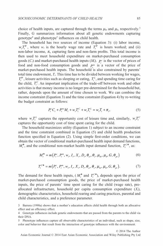
choice of health inputs, are captured through the terms μht and μh, respectively.3

Finally, G summarizes information about all genetic endowments capturinggenotype4 and phenotype5 influences on child health.

The household has two sources of income (Equation 3): (i) labor income,w Tt t

W , where wt is the hourly wage rate and TtW is hours worked; and (ii)

non-labor income, πt, capturing farm and non-farm profits. This total income isthen used to meet household expenditure on market-purchased consumptiongoods (Ct) and market-purchased health inputs (Mt). Pt

c is the vector of prices offood and non-food consumption goods and Pt

m is a vector of the price ofmarket-purchased health inputs. The household is also constrained by parents’total time endowment, Tt. This time has to be divided between working for wages,Tt

W , leisure activities such as sleeping or eating, TtL, and spending time caring for

the child, TtC. An important implication of the trade-off between work and other

activities is that money income is no longer pre-determined for the household but,rather, depends upon the amount of time chosen to work. We can combine theincome constraint (Equation 3) and the time constraint (Equation 4) by re-writingthe budget constraint as follows:

P C P M w T w T w Ttc

t tm

t t tC

t tL

t t t+ + + = + π , (5)

where w Tt tL captures the opportunity cost of leisure time and, similarly, w Tt t

C

captures the opportunity cost of time spent caring for the child.The household maximizes utility (Equation 1) subject to an income constraint

and the time constraint combined in Equation (5) and child health productionfunction specified in Equation (2). Using simple first-order conditions, we canobtain the vector of conditional market-purchased health input demand functions,Mt

*, and the conditional non-market health input demand function, TtC*, as:

M m P P w I X D Gt tc

tm

t t t t ct c ht h pt* , , , , , , , , , , ,= ( )θ θ μ μ θ (6)

T m P P w I X D GtC

tc

tm

t t t t ct c ht h pt* , , , , , , , , , , , .= ( )θ θ μ μ θ (7)

The demand for these health inputs, ( Mt* and Tt

C*), depends upon the price ofmarket-purchased consumption goods, the price of market-purchased healthinputs, the price of parents’ time spent caring for the child (wage rate), pre-allocated infrastructure, household per capita consumption expenditure (Xt),demographic characteristics, household rearing and caring practices, parental andchild characteristics, and a preference parameter.

3 Barrera (1990a) shows that a mother’s education affects child health through both an allocativeeffect and an efficiency effect.4 Genotype influences include genetic endowments that are passed from the parents to the child viatheir DNA.5 Phenotype influences capture all observable characteristics of an individual, such as shape, size,color and behavior that result from the interaction of genotype influences with the environment.



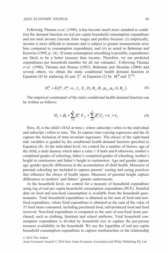
Following Thomas et al. (1990), it has become much more standard to condi-tion the demand function on real per capita household consumption expenditureand not total income (income from wages and profits) because: (i) empirically,income is more difficult to measure and is subject to greater measurement errorbias compared to consumption expenditure; and (ii) as noted in Behrman andKnowles (1999, p. 14), ‘If some consumption smoothing is possible, expendituresare likely to be a better measure than income. Therefore, we use predictedexpenditures per household member for all our estimates’. Following Thomaset al. (1990), Thomas and Strauss (1992), Behrman and Skoufias (2004) andseveral others, we obtain the static conditional health demand function inEquation (8) by replacing Mt and Tt

C in Equation (2) by Mt* and Tt

C*:

H h P P w I X D Gt tc

tm

t t t t ct c ht h pt* , , , , , , , , , , , .= ( )θ θ μ μ θ (8)

The empirical counterpart of the static conditional health demand function canbe written as follows:

H X Zit jX

jitj

R

jZ

jij

S

c it= + + + += =

∑ ∑β β β ε ε01 1

(9)

Here, Hit is the child’s HAZ at time t, where subscript i refers to the individualand subscript t refers to time. The Xs capture time-varying regressors and the Zscapture the inclusion of time-invariant regressors. The choice of the right-handside variables is guided by the conditional health demand function specified inEquation (8). At the individual level, we control for a number of factors: age ofthe child, a male dummy which takes a value 1 if male and 0 otherwise, mother’scompleted grades of schooling, father’s completed grades of schooling, mother’sheight in centimeters and father’s height in centimeters. Age and gender captureage–gender specific differences in the accumulation of child health. Measures ofparental schooling are included to capture parents’ rearing and caring practicesthat influence the choice of health inputs. Measures of parental height capturedifferences in mothers’ and fathers’ genetic endowments.

At the household level, we control for a measure of household expenditureusing log of real per capita household consumption expenditure (PCE). Detaileddata on food and non-food consumption is available from the household ques-tionnaire. Total household expenditure is obtained as the sum of food and non-food expenditure, where food expenditure is obtained as the sum of the value of35 food items consumed, including purchased food, self-produced food and foodreceived. Non-food expenditure is computed as the sum of non-food items pur-chased, such as clothing, furniture and school uniforms. Total household con-sumption expenditure is divided by household size to capture the per-personresource availability in the household. We use the logarithm of real per capitahousehold consumption expenditure to capture nonlinearities in the relationship



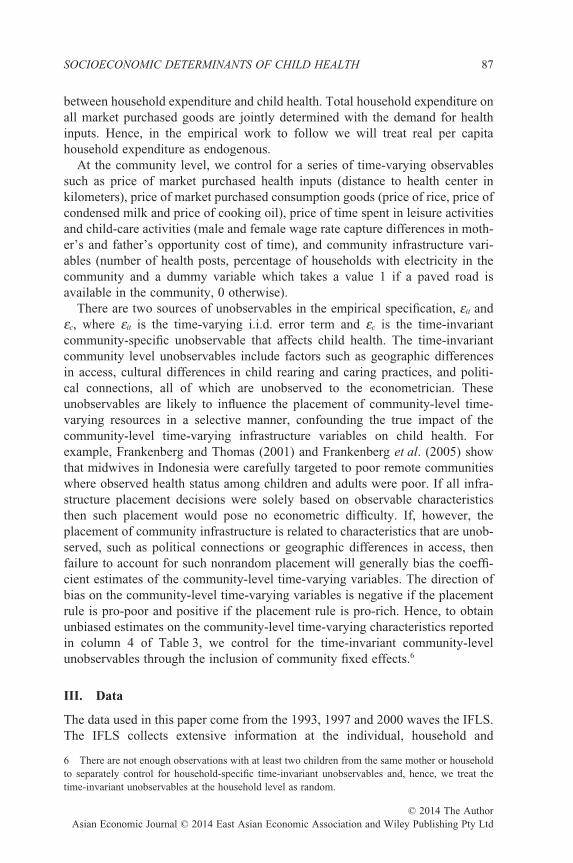
between household expenditure and child health. Total household expenditure onall market purchased goods are jointly determined with the demand for healthinputs. Hence, in the empirical work to follow we will treat real per capitahousehold expenditure as endogenous.

At the community level, we control for a series of time-varying observablessuch as price of market purchased health inputs (distance to health center inkilometers), price of market purchased consumption goods (price of rice, price ofcondensed milk and price of cooking oil), price of time spent in leisure activitiesand child-care activities (male and female wage rate capture differences in moth-er’s and father’s opportunity cost of time), and community infrastructure vari-ables (number of health posts, percentage of households with electricity in thecommunity and a dummy variable which takes a value 1 if a paved road isavailable in the community, 0 otherwise).

There are two sources of unobservables in the empirical specification, εit andεc, where εit is the time-varying i.i.d. error term and εc is the time-invariantcommunity-specific unobservable that affects child health. The time-invariantcommunity level unobservables include factors such as geographic differencesin access, cultural differences in child rearing and caring practices, and politi-cal connections, all of which are unobserved to the econometrician. Theseunobservables are likely to influence the placement of community-level time-varying resources in a selective manner, confounding the true impact of thecommunity-level time-varying infrastructure variables on child health. Forexample, Frankenberg and Thomas (2001) and Frankenberg et al. (2005) showthat midwives in Indonesia were carefully targeted to poor remote communitieswhere observed health status among children and adults were poor. If all infra-structure placement decisions were solely based on observable characteristicsthen such placement would pose no econometric difficulty. If, however, theplacement of community infrastructure is related to characteristics that are unob-served, such as political connections or geographic differences in access, thenfailure to account for such nonrandom placement will generally bias the coeffi-cient estimates of the community-level time-varying variables. The direction ofbias on the community-level time-varying variables is negative if the placementrule is pro-poor and positive if the placement rule is pro-rich. Hence, to obtainunbiased estimates on the community-level time-varying characteristics reportedin column 4 of Table 3, we control for the time-invariant community-levelunobservables through the inclusion of community fixed effects.6

III. Data

The data used in this paper come from the 1993, 1997 and 2000 waves the IFLS.The IFLS collects extensive information at the individual, household and

6 There are not enough observations with at least two children from the same mother or householdto separately control for household-specific time-invariant unobservables and, hence, we treat thetime-invariant unobservables at the household level as random.



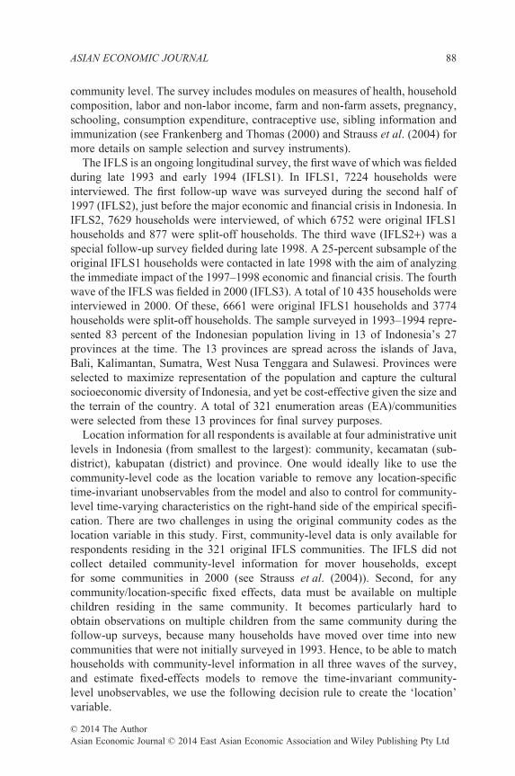
community level. The survey includes modules on measures of health, householdcomposition, labor and non-labor income, farm and non-farm assets, pregnancy,schooling, consumption expenditure, contraceptive use, sibling information andimmunization (see Frankenberg and Thomas (2000) and Strauss et al. (2004) formore details on sample selection and survey instruments).

The IFLS is an ongoing longitudinal survey, the first wave of which was fieldedduring late 1993 and early 1994 (IFLS1). In IFLS1, 7224 households wereinterviewed. The first follow-up wave was surveyed during the second half of1997 (IFLS2), just before the major economic and financial crisis in Indonesia. InIFLS2, 7629 households were interviewed, of which 6752 were original IFLS1households and 877 were split-off households. The third wave (IFLS2+) was aspecial follow-up survey fielded during late 1998. A 25-percent subsample of theoriginal IFLS1 households were contacted in late 1998 with the aim of analyzingthe immediate impact of the 1997–1998 economic and financial crisis. The fourthwave of the IFLS was fielded in 2000 (IFLS3). A total of 10 435 households wereinterviewed in 2000. Of these, 6661 were original IFLS1 households and 3774households were split-off households. The sample surveyed in 1993–1994 repre-sented 83 percent of the Indonesian population living in 13 of Indonesia’s 27provinces at the time. The 13 provinces are spread across the islands of Java,Bali, Kalimantan, Sumatra, West Nusa Tenggara and Sulawesi. Provinces wereselected to maximize representation of the population and capture the culturalsocioeconomic diversity of Indonesia, and yet be cost-effective given the size andthe terrain of the country. A total of 321 enumeration areas (EA)/communitieswere selected from these 13 provinces for final survey purposes.

Location information for all respondents is available at four administrative unitlevels in Indonesia (from smallest to the largest): community, kecamatan (sub-district), kabupatan (district) and province. One would ideally like to use thecommunity-level code as the location variable to remove any location-specifictime-invariant unobservables from the model and also to control for community-level time-varying characteristics on the right-hand side of the empirical specifi-cation. There are two challenges in using the original community codes as thelocation variable in this study. First, community-level data is only available forrespondents residing in the 321 original IFLS communities. The IFLS did notcollect detailed community-level information for mover households, exceptfor some communities in 2000 (see Strauss et al. (2004)). Second, for anycommunity/location-specific fixed effects, data must be available on multiplechildren residing in the same community. It becomes particularly hard toobtain observations on multiple children from the same community during thefollow-up surveys, because many households have moved over time into newcommunities that were not initially surveyed in 1993. Hence, to be able to matchhouseholds with community-level information in all three waves of the survey,and estimate fixed-effects models to remove the time-invariant community-level unobservables, we use the following decision rule to create the ‘location’variable.



The ‘location’ variable created here is assigned a community code wheneverthere are 5 or more children residing in the same community.7 In cases where thiscriterion fails, the ‘location’ variable is assigned the code corresponding to thenext level of aggregation, (i.e. the kecamatan)8 code following the same rules.Similarly, the kabupatan and, lastly, the province codes are assigned to thelocation variable in order to obtain at least 5 children from each of the newly-created location variables. This new aggregation of the geographic units helps uscombine household-level and community-level information and also allows theuse of fixed-effects estimation techniques at the location level. It is this ‘location’variable that captures geographic information corresponding to each household inall three waves of the IFLS. All community-level characteristics reported in thetables vary at the location level created in this paper and not at the originalcommunity i.d. level.

Despite the availability of one more wave of data from the IFLS administeredin 2007, we restrict our sample to only include children under the age of 5 yearsin 1993 following them through to the 1997 and 2000 but not the 2007 waves ofthe IFLS. There are several reasons for doing this. First, Martorell and Habicht(1986) and Satyanarayana et al. (1989) point out that a decline in growth in heightduring the first few years of life largely determines the small stature exhibitedby adults in developing countries. Second, height measured at a young age isstrongly correlated with adult body size (Spurr, 1988; Martorell, 1995). Third, theaverage age of a child in our sample in 1993 is 3 years. By 2000, the average ageof a child in our sample is 10 years. The next wave of the IFLS is only availablefor 2007, by which time a majority of these children are likely to have reachedtheir final height and can no longer be influenced by the socioeconomic factorscollected at the time of the survey. In addition, the literature on human biologyindicates that most of the growth in height that occurs during adolescence (ages13 and above) is caused by individual-specific growth spurts that occur at adifferent time for each child as they enter puberty. The height gain observedamong children in adolescence is further attributable to only these unobservedindividual-specific growth spurts and not their socioeconomic environment. Con-sequently, it limits what we can learn from estimating conditional demand func-tions for this sample. Furthermore, height gains during pubertal growth spurts arenot enough to reverse the negative consequences of early life stunting amongchildren (Satyanarayana et al., 1980, 1989). For these reasons, we restrict ouranalysis to only follow children under the age of 5 years in 1993 through the 1997

7 It is usually the case that fewer than 5 children are found only in communities that were not theoriginal IFLS1 communities and are communities where mover households resided.8 The kecamatan and kabupatan codes are based on Indonesian Central Bureau of Statistics (BPS)codification that can be easily linked to other national data like the SUSENAS. The definition of akecamatan and a kabupatan continue to change over time. In order to use systematic codes of thekecamatan and kabupatan over time, I use the 1999 BPS codes that define the kecamatan and kabuptancodes for all IFLS communities from all 3 years of the survey.



and 2000 waves of the IFLS when surrounding socioeconomic factors have thepotential to influence a child’s growth process.

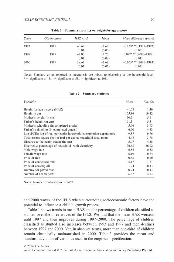
Table 1 shows trends in mean HAZ and the percentage of children classified asstunted over the three waves of the IFLS. We find that the mean HAZ worsensuntil 1997 and then improves during 1997–2000. The percentage of childrenclassified as stunted also increases between 1993 and 1997 and then declinesbetween 1997 and 2000. Yet, in absolute terms, more than one-third of childrenremain chronically malnourished in 2000. Table 2 provides the mean andstandard deviation of variables used in the empirical specification.

Table 1 Summary statistics on height-for-age z-score

Years Observations HAZ < −2 Mean Mean difference (years)

1993 1819 40.62 −1.62 −0.133*** (1997–1993)(0.01) (0.03) (0.03)

1997 1819 42.05 −1.75 0.077*** (2000–1997)(0.01) (0.02) (0.01)

2000 1819 38.64 −1.68 −0.055*** (2000–1993)(0.01) (0.02) (0.03)

Notes: Standard errors reported in parenthesis are robust to clustering at the household level.*** significant at 1%, ** significant at 5%, * significant at 10%.

Table 2 Summary statistics

Variables Mean Std. dev

Height-for-age z-score (HAZ) −1.68 1.30Height in cm 105.86 19.42Mother’s height (in cm) 150.5 5.1Father’s height (in cm) 161.3 5.3Mother’s schooling (in completed grades) 5.96 3.93Father’s schooling (in completed grades) 6.90 4.33Log (PCE): log of real per capita household consumption expenditure 9.87 0.76Total assets: square root of real per capita household total assets 4.48 3.78Distance to the health center (in km) 5.07 4.58Electricity: percentage of households with electricity 76.68 26.92Male wage rate 6.55 0.52Female wage rate 6.19 0.84Price of rice 0.85 0.20Price of condensed milk 5.17 1.51Price of cooking oil 1.74 0.43Dummy for paved road 0.74 0.43Number of health posts 6.67 4.73

Notes: Number of observations: 5457.



IV. Results

Ordinary least square estimates of the determinants of child health are presentedin columns 1 and 2 of Table 3, where households’ long-run resource availabilityis captured using log(PCE) in column 1, Table 3 and total assets in column 2,Table 3. The preferred instrumental variable (IV) estimates for log(PCE) arereported in columns 3 and 4 of Table 3. The results reported in column 3, Table 3include the full set of community/location interacted time dummies to control forall possible time-varying community-level factors both observable and unobserv-able to the econometrician at date t. In contrast in column 4, Table 3 we replacethese community interacted time dummies with actual community level time-varying observable characteristics such as price of food consumption goods,distance to health center and other observables reported in column 4, Table 3.While the estimates reported in both columns 3 and 4 of Table 3 result in unbiasedestimates for the household and child-level characteristics, there is no informationon observable time-varying community characteristics in column 3, which arepresented in column 4, Table 3. The estimates reported in column 4, Table 3 aremore useful for policy prescription, because they identify the impact of variouscommunity characteristics on child health.9 White’s heteroskedasticity robuststandard errors adjusted for clustering at the individual level are reported inTable 3 (Wooldridge, 2002).

We assume that the coefficient estimates on the right-hand side variables do notdiffer by gender. To check this assumption, we report the results from pooling themale and female sample together. The χ2 test of pooling results in a value of 32.46(p-value = 0.05) and favors separating the sample for boys from girls. However,a χ2 test on all the right-hand side variables except the age and gender-interactedcoefficients results in a value of 24.79 (p-value = 0.16), which further suggeststhat the gender-specific differences in the determinants of child health only comefrom the presence of age and gender-specific differences in growth of height.Hence, the preferred estimates reported in Table 3 use the pooled sample of boysand girls together, controlling for age, gender and interactions thereof to accountfor age and gender-specific differences in children’s health outcomes.

The coefficient on the male dummy reported in column 4, Table 3 has anegative sign, suggesting that female children have better health than male chil-dren. This result is striking when compared to other Asian countries like India andBangladesh which exhibit comparable levels of stunting, where one finds largesignificant gender differentials in favor of boys vis-a-vis girls. For Indonesia, thisis not particularly surprising, because the country does not traditionally sufferfrom large gender differential investments in human capital accumulation. Inexamining mortality rates, Kevane and Levine (2001) find no evidence of‘missing girls’; that is, daughters are not likely to suffer from higher rates ofmortality as compared to sons. Levine and Ames (2003) show that even in theaftermath of the crisis, girls did not fare worse than boys.

9 The terms location and community are used interchangeably throughout the paper.



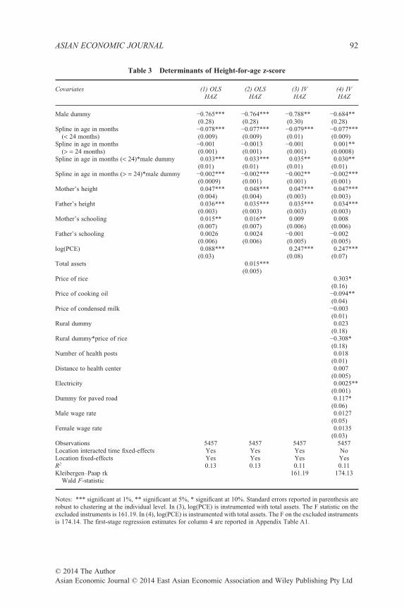
Table 3 Determinants of Height-for-age z-score

Covariates (1) OLS (2) OLS (3) IV (4) IVHAZ HAZ HAZ HAZ

Male dummy −0.765*** −0.764*** −0.788** −0.684**(0.28) (0.28) (0.30) (0.28)

Spline in age in months(< 24 months)

−0.078*** −0.077*** −0.079*** −0.077***(0.009) (0.009) (0.01) (0.009)

Spline in age in months(> = 24 months)

−0.001 −0.0013 −0.001 0.001**(0.001) (0.001) (0.001) (0.0008)

Spline in age in months (< 24)*male dummy 0.033*** 0.033*** 0.035** 0.030**(0.01) (0.01) (0.01) (0.01)

Spline in age in months (> = 24)*male dummy −0.002*** −0.002*** −0.002** −0.002***(0.0009) (0.001) (0.001) (0.001)

Mother’s height 0.047*** 0.048*** 0.047*** 0.047***(0.004) (0.004) (0.003) (0.003)

Father’s height 0.036*** 0.035*** 0.035*** 0.034***(0.003) (0.003) (0.003) (0.003)

Mother’s schooling 0.015** 0.016** 0.009 0.008(0.007) (0.007) (0.006) (0.006)

Father’s schooling 0.0026 0.0024 −0.001 −0.002(0.006) (0.006) (0.005) (0.005)

log(PCE) 0.088*** 0.247*** 0.247***(0.03) (0.08) (0.07)

Total assets 0.015***(0.005)

Price of rice 0.303*(0.16)

Price of cooking oil −0.094**(0.04)

Price of condensed milk −0.003(0.01)

Rural dummy 0.023(0.18)

Rural dummy*price of rice −0.308*(0.18)

Number of health posts 0.018(0.01)

Distance to health center 0.007(0.005)

Electricity 0.0025**(0.001)

Dummy for paved road 0.117*(0.06)

Male wage rate 0.0127(0.05)

Female wage rate 0.0135(0.03)

Observations 5457 5457 5457 5457Location interacted time fixed-effects Yes Yes Yes NoLocation fixed-effects Yes Yes Yes YesR2 0.13 0.13 0.11 0.11Kleibergen–Paap rk

Wald F-statistic161.19 174.13

Notes: *** significant at 1%, ** significant at 5%, * significant at 10%. Standard errors reported in parenthesis arerobust to clustering at the individual level. In (3), log(PCE) is instrumented with total assets. The F statistic on theexcluded instruments is 161.19. In (4), log(PCE) is instrumented with total assets. The F on the excluded instrumentsis 174.14. The first-stage regression estimates for column 4 are reported in Appendix Table A1.



The relationship between HAZ and age in months is nonlinear and thecoefficient on the spline variables captures this nonlinearity, indicating thatz-scores decline until the age of 24 months and then improve and remain steadyand or unchanged after 48 months.10 The interaction terms between the splinevariables and the male dummy capture the age and gender-specific changes inhealth outcomes.

Household characteristics included in the regression model are: mother’s com-pleted grades of schooling, father’s completed grades of schooling, mother’sheight in centimeters, father’s height in centimeters, and log of real per capitaconsumption expenditure. Measures of parental schooling capture the efficiencywith which health inputs are transformed into health outputs (Barrera, 1990a;Strauss and Thomas, 1998; Fedorov and Sahn, 2005). The coefficient estimates onmother’s completed grades of schooling and father’s completed grades of school-ing reported in column 1, Table 3 show an expected positive relationship betweenparental schooling and child health. Every additional year of mother’s schoolingincreases z-scores by 0.015 (column 1, Table 3) standard deviations. Father’sschooling has a positive, although insignificant impact on z-scores. The positivecorrelation between household per capita consumption expenditure and mother’sschooling is likely to have biased the coefficient estimate on mother’s schoolingupwards in column 1, Table 3. The preferred IV estimates reported in column 4,Table 3 suggest, however, that neither of the parental schooling variables have astatistically significant impact on child health.

Measures of parental height capture the impact of genetic endowments on childhealth (Strauss and Thomas, 1998). Mother’s height in centimeters and father’sheight in centimeters capture the role of parent-specific genetic endowments onchild health.11 Every 1-cm increase in mother’s height (father’s height) is asso-ciated with a 0.047 (0.034) standard deviation improvement in HAZ (column 4,Table 3). These results are consistent with earlier findings in the literature(Ghuman et al., 2005; Thomas et al., 1991).

The final household characteristic included in the regression specification ishousehold income. Logarithm of real per capita household consumption expen-diture [log (PCE)] is used to capture the household’s access to resources inthe long run. OLS estimates of log(PCE) from column 1, Table 3 can be bothbiased upwards due to its correlation with time-invariant household-specificunobservables and biased downwards due to measurement error in data. Becauseassets are exogenously determined in a static model we replace log(PCE) withtotal assets in column 2 of Table 3. The coefficient estimates on log(PCE) andassets reported in Table 3 suggest that children residing in households with higherincome enjoy better health. The IV estimates of log(PCE) is reported in columns3 and 4 of Table 3 where log(PCE) is instrumented with the sum of household

10 This is consistent with much of the literature on health outcomes (see Strauss et al., 2004).11 See Thomas and Strauss (1992) for discussion on the role played by parent-specific geneticendowments in explaining child health.



productive assets, unproductive assets and unearned income (which sum up tototal assets), which are assumed to be exogenous in a static model. The coefficientestimate on log(PCE) increases from 0.08 (column 1, Table 3) to 0.24 (columns3 and 4, Table 3), showing that IV estimates of income have a much larger impacton current health status. The increase in the coefficient estimate of log(PCE) fromOLS to IV regressions indicates that OLS estimates of log(PCE) are likely to bebiased downward due to measurement error and not biased upwards due toomitted variables.12 The role of income is largely consistent with most relatedwork examining the determinants of child health.13 Household income can alsopossibly have nonlinear effects on child health. To capture this nonlinearity, weinclude a spline in the measure of household income at the sample median. Thepreferred IV specification is re-estimated with the nonlinear measures oflog(PCE). The two measures of log(PCE) in the nonlinear specification are notsignificantly different from each other. A chi2 test on the two measures oflog(PCE) is 0.48 (p-value = 0.48), rejecting any nonlinear effect of log(PCE) onchild health.

The role of time-varying community/location characteristics is also importantin determining child health. In the presence of endogenous program placementeffects, failure to take into account the correlation between community infrastruc-ture variables and community-level time-invariant unobservables can bias coef-ficient estimates on the community characteristics (Rosenzweig and Wolpin,1986; Frankenberg et al., 2005). To address this issue the preferred IV estimatesinclude location fixed effects that allow us to identify the exogenous impact of thetime-varying community-level characteristics on child health. These estimates arevalid under the assumption that the time-varying community-level unobserv-ables that affect program placement are uncorrelated with the community-levelobservable characteristics. The panel structure of our data allows us to obtainunbiased parameter estimates on both the family background characteristics aswell as time-varying community characteristics controlling for community-levelfixed effects (see column 4, Table 3). This is usually not possible with cross-sectional data because community fixed effects would also sweep out thecommunity-level variables included in the empirical specification, as in Ghumanet al. (2005).14

Among the community-level time-varying characteristics, we find that anincrease in the price of rice is associated with improvements in child health inurban areas (0.303), while it has a negative impact in rural areas (–0.005) (column

12 The F-statistics on the excluded instruments in the first-stage regression for the IV estimatesreported in Table 3 are appended at the end of Table 3, and the complete first-stage regressionestimates are summarized in Appendix Table A1.13 Thomas et al. (1991), Thomas and Strauss (1992), Haddad et al. (2003), Glick and Sahn (1998),Sahn (1994) and Thomas et al. (1990) all find a strong positive effect of per capita consumptionexpenditure in determining child health.14 Ghuman et al. (2005) are able to obtain reliable estimates of the household-specific observablesas they control for village fixed effects.



4, Table 3). The effect, however, is statistically significant only at the 10-percentsignificance level. Although this result might seem surprising and counterintuitiveat first glance, it is not so in the context of Indonesia. For instance, Alderman andTimmer (1980) find a higher income elasticity of demand with respect to riceconsumption in rural Indonesia compared to urban areas. Ito et al. (1989) andBouis (1991) find that urban households in Indonesia are more likely to choosehigh quality, more nutritious substitutes for rice. These findings suggest that ruralIndonesians are more price sensitive and, hence, are likely to witness a decline inchild health that is affected by an increase in rice price, whereas urban Indone-sians are able to find more nutritious substitutes for rice, which results in improve-ments in child HAZ, as observed here. Finally, urban households in Indonesiaallocate only one-fifth of their household budget share to staples (primarily rice),while rural households allocate two-fifths of their household budget share tostaples; consequently, the substitution effect of an increase in rice price is greaterfor rural areas, as observed here (Thomas et al., 1999).

An increase in the price of cooking oil is associated with a decline in childhealth (column 4, Table 3). Expenditure on cooking oil may not be a largeproportion of total household consumption expenditure but reflects spending onessential consumption goods. One important consumption good aimed only forchildren is condensed milk; it is also included in the regression results. Theadvantage of using condensed milk is that it does not need refrigeration, animportant advantage in a country where not all households own a refrigerator. Theprice of condensed milk has a positive but insignificant impact in determiningchild health. We acknowledge that a range of consumption goods must beincluded in the right-hand side. However, data constraints do not allow us tocontrol for prices of more consumption goods.

In addition, included in the regressions are prices of health inputs as capturedby distance to health center, and price of parents’ time as captured by male andfemale-specific hourly wage rates in a community. None of these have a statis-tically significant impact on child health. We find some degree of positive cor-relation between male and female wage rates (the Spearman rank correlationcoefficient is 0.47; see Appendix Table A2) weakening the independent effect ofthese variables on child HAZ. However, notice that in Appendix Table A2, thecorrelation coefficient between all the community variables is fairly small and,hence, there is no evidence of multicollinearity.

Measures of community infrastructure availability such as the number of healthposts (access to health care), presence of paved roads (access to bigger cities) andmeasure of electricity (storage facility) are used as additional control variables.The number of health posts in a community has a positive but insignificant impacton child health. Measures for presence of paved roads and measure of electricityin the community are both positively associated with improvements in childhealth. Children residing in communities with a paved road have 0.11 standarddeviation higher z-scores compared to their counterparts residing in communitieswithout a paved road. Similarly, children residing in communities with greater



prevalence of electricity on average gain a 0.0025 standard deviation improve-ment in z-scores.

A number of the community-level time-varying factors, such as male andfemale wage rates, number of health posts, distance to health center and price ofcondensed milk, have no significant impact on child health. One possible expla-nation for this is that a lot of the variation in the community time-varyingvariables in our panel comes from variation across communities that gets pickedup by the community fixed effects rather than variation over time within com-munities. To check for this we decompose the variation in the community vari-ables into two parts: the proportion of variation across communities and theproportion of variation within communities. We regress the community-levelmale wage rate on the full set of community dummies and obtain an associatedR2 of 0.70. This R2 tells us that 70 percent of the variation in male wages iscoming from variation across communities and that only 30 percent of thevariation in male wages comes from variation within the community. We conducta similar exercise for all the time-varying community variables where the pro-portion of across and within community variation is given in Appendix Table A3.Notice that for all the community variables that are insignificant in column 4,Table 3, the majority of the variation in these variables is coming from variationacross communities which gets picked up by the community fixed effects, leavingout the limited over time variation to be picked by the community level variablesincluded in column 4, Table 3.

Using the final preferred estimates reported in column 4, Table 3, we conducta simple simulation exercise to outline the policy implications of this paper.Notice that the coefficient estimate reported in column 4, Table 3 suggests thata 1-cm increase in mother’s height (father’s height) is associated with a 0.047(0.034) standard deviation improvement in child HAZ. First, the averagemother’s height in our sample is 150.53 cm and the average height of a motherwhose children are not stunted is 151.58 cm. Now, if we were to assume thatall mothers in our sample have the height of a well-nourished child’s motherthen average mother’s height in the sample would increase by 1 cm and, as aresult, the predicted HAZ will also increase by 0.047 standard deviations. Asimilar policy simulation can be conducted with father’s height; that is, ifall children in our sample were to now have the height of a well-nourishedchild’s father’s height then the predicted HAZ for children would increase by0.034 standard deviations. Second, access to paved roads increases the pre-dicted HAZ by 0.117 standard deviations. In our sample, only 80 percent ofhouseholds have access to paved roads. Now if all households were to haveaccess to paved roads, that is, the variable paved road now takes a value of 1for everyone in the sample, then the predicted HAZ will increase further by0.023 standard deviations. Finally, we can simulate the impact 100 percentaccess to electricity on the predicted HAZ. We find that increasing access toelectricity from 75 to 100 percent in Indonesia will increase predicted HAZ by0.06 standard deviations.



The findings in the paper suggest that governments and policy-makers need toguide investments in programs and policies that lead to improvements in house-hold income, parents’ height (through improvements in children’s height todaywhich will have intergenerational effects), access to paved roads and electricitythat will lead to improvements in HAZ.

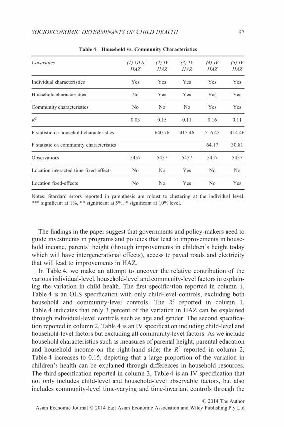
In Table 4, we make an attempt to uncover the relative contribution of thevarious individual-level, household-level and community-level factors in explain-ing the variation in child health. The first specification reported in column 1,Table 4 is an OLS specification with only child-level controls, excluding bothhousehold and community-level controls. The R2 reported in column 1,Table 4 indicates that only 3 percent of the variation in HAZ can be explainedthrough individual-level controls such as age and gender. The second specifica-tion reported in column 2, Table 4 is an IV specification including child-level andhousehold-level factors but excluding all community-level factors. As we includehousehold characteristics such as measures of parental height, parental educationand household income on the right-hand side; the R2 reported in column 2,Table 4 increases to 0.15, depicting that a large proportion of the variation inchildren’s health can be explained through differences in household resources.The third specification reported in column 3, Table 4 is an IV specification thatnot only includes child-level and household-level observable factors, but alsoincludes community-level time-varying and time-invariant controls through the

Table 4 Household vs. Community Characteristics

Covariates (1) OLS (2) IV (3) IV (4) IV (5) IVHAZ HAZ HAZ HAZ HAZ

Individual characteristics Yes Yes Yes Yes Yes

Household characteristics No Yes Yes Yes Yes

Community characteristics No No No Yes Yes

R2 0.03 0.15 0.11 0.16 0.11

F statistic on household characteristics 640.76 415.46 516.45 414.46

F statistic on community characteristics 64.17 30.81

Observations 5457 5457 5457 5457 5457

Location interacted time fixed-effects No No Yes No No

Location fixed-effects No No Yes No Yes

Notes: Standard errors reported in parenthesis are robust to clustering at the individual level.*** significant at 1%, ** significant at 5%, * significant at 10% level.



inclusion of the location dummies and the location-interacted time dummiescontrolling for both endogenous program placement effects and communitytime-varying factors. These controls result in an R2 of 0.11, indicating that notmuch of the explained variation in HAZ comes from variation in community-level factors. The specification reported in column 3, Table 4 is theoreticallyappropriate except that from a policy point of view, it does not have informationon the influence of community-level factors on child health. The fourth specifi-cation reported in column 4, Table 4 is an IV specification with individual-level,household-level and community-level controls but does not address the problemof endogenous program placement. As we add community-level observables incolumn 4, Table 4 the R2 only increases marginally to 0.16, depicting that only avery small proportion of the variation in children’s health comes from variation incommunity resources. The changes in the R2 across specifications suggest that incomparison to community characteristics, household characteristics are morepowerful in explaining variation in children’s health. The last specificationreported in column 5, Table 4 is an IV specification with the full set of individual,household and community-level controls. It also includes a set of community/location dummies to sweep out the program placement effects and results in an R2

of 0.11; this is closer to the R-square reported in column 2, Table 4 with only thehousehold-level and child-level controls.

The theoretical model outlined in the paper identifies the best specification asthe one including the full set of time-varying and time-invariant community-level,household-level and individual-level factors as appropriate controls on the right-hand side of the empirical specification. Using this as a guide, we can say thatboth the specifications reported in columns 3 and 5 of Table 4 (analogous to thespecifications reported in columns 3 and 4 of Table 3) are theoretically justified.However, there is more information (in the form of community-level time-varying factors) to learn from the empirical specification reported in column 5,Table 4 that is otherwise absorbed in the community-time fixed-effects reportedin column 3, Table 4. Overall, changes in the value of R-square reported acrossspecifications suggest that in comparison to community characteristics, house-hold characteristics are more powerful in explaining variation in children’shealth.

V. Conclusion

This paper characterizes the socioeconomic determinants of child health usingdata on HAZ, a long-run measure of chronic nutritional deficiency. Panel dataare constructed using observations on children initially between ages 3 and 59months in 1993 followed through the 1997 and 2000 waves of the IFLS. A staticconditional health demand function is estimated to obtain the parameter estimateson the various child-level, household-level and community-level factors thataffect child health in Indonesia.



Our findings indicate that household income has a large and statistically sig-nificant role in explaining improvements in children’s health. OLS estimates ofthe impact of household income are biased downwards relative to IV results. Wealso find a strong positive association between parental height and children’shealth. At the community level, we find that provision of electricity andavailability of a paved road is positively associated with improvements in chil-dren’s health. Finally, we find that in comparison to community-level factors,household-level characteristics are more important in explaining improvements inchildren’s health. Finally, there is no evidence of gender-specific differences inthe determinants of HAZ in Indonesia.

The key policy implication of this paper is that investment in programs thatincrease household income, parent’s height (through investments in child heighttoday) and community infrastructure are likely to improve children’s health, and,consequently, their education and earnings in the long run. At the household level,government’s can provide cash transfers and offer employment opportunities toaugment household income. Finally, improvements in access to paved roads andelectricity at the community level will contribute towards improving children’shealth.



Appendix

Table A1 First-stage regression results

Excluded and included instruments from thefirst-stage regressions

coefficient estimates on the first-stageregressions variables reported

in column 4, table 3

excluded instrumentsTotal assets 0.06***

(0.004)included instrumentsMale dummy 0.05

(0.08)Spline in age in months (< 24 months) 0.007**

(0.002)Spline in age in months (> = 24 months) −0.001***

(0.0004)Spline in age in months (< 24)*male dummy −0.003

(0.004)Spline in age in months (> = 24)*male dummy 0.0005

(0.0004)Mother’s height 0.002

(0.001)Father’s height 0.002

(0.001)Mother’s schooling 0.02***

(0.003)Father’s schooling 0.01***

(0.003)Price of rice −0.22***

(0.07)Price of cooking oil 0.14***

(0.02)Price of condensed milk 0.003

(0.007)Rural dummy −0.32***

(0.08)Rural dummy*price of rice 0.15*

(0.08)Number of health posts −0.0003

(0.002)Distance to health center −0.007

(0.002)Electricity −0.0002

(0.0005)Dummy for paved road 0.004

(0.02)Male wage rate 0.06**

(0.02)Female wage rate 0.03**

(0.01)Observations 5457Location fixed-effects YesF statistic on the excluded instruments from

the first-stage regressions174.14

*** significant at 1%, ** significant at 5%, * significant at 10%.



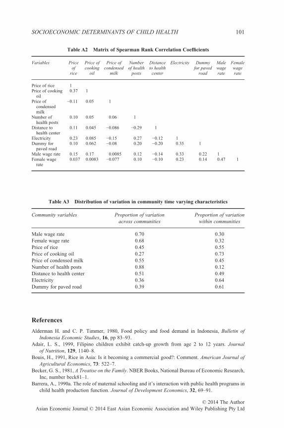
Table A2 Matrix of Spearman Rank Correlation Coefficients

Variables Priceof

rice

Price ofcooking

oil

Price ofcondensed

milk

Numberof health

posts

Distanceto health

center

Electricity Dummyfor paved

road

Malewagerate

Femalewagerate

Price of rice 1Price of cooking

oil0.37 1

Price ofcondensedmilk

−0.11 0.05 1

Number ofhealth posts

0.10 0.05 0.06 1

Distance tohealth center

0.11 0.045 −0.086 −0.29 1

Electricity 0.23 0.085 −0.15 0.27 −0.12 1Dummy for

paved road0.10 0.062 −0.08 0.20 −0.20 0.35 1

Male wage rate 0.15 0.17 0.0085 0.12 −0.14 0.33 0.22 1Female wage

rate0.037 0.0083 −0.077 0.10 −0.10 0.23 0.14 0.47 1

Table A3 Distribution of variation in community time varying characteristics

Community variables Proportion of variationacross communities

Proportion of variationwithin communities

Male wage rate 0.70 0.30Female wage rate 0.68 0.32Price of rice 0.45 0.55Price of cooking oil 0.27 0.73Price of condensed milk 0.55 0.45Number of health posts 0.88 0.12Distance to health center 0.51 0.49Electricity 0.36 0.64Dummy for paved road 0.39 0.61

References

Alderman H. and C. P. Timmer, 1980, Food policy and food demand in Indonesia, Bulletin oflndonesia Economic Studies, 16, pp 83–93.

Adair, L. S., 1999, Filipino children exhibit catch-up growth from age 2 to 12 years. Journalof Nutrition, 129, 1140–8.

Bouis, H., 1991, Rice in Asia: Is it becoming a commercial good?: Comment. American Journal ofAgricultural Economics, 73: 522–7.

Becker, G. S., 1981, A Treatise on the Family. NBER Books, National Bureau of Economic Research,Inc, number beck81–1.

Barrera, A., 1990a. The role of maternal schooling and it’s interaction with public health programs inchild health production function. Journal of Development Economics, 32, 69–91.



Barrera, A., 1990b, The interactive effects of mother’s schooling and unsupplemented breastfeedingon child health. Journal of Development Economics, 34, 81–98.

Behrman, J. R. and A. B. Deolalikar, 1988, Health and nutrition, Handbook of DevelopmentEconomics, In: Handbook of Development Economics, edition 1, volume 1 (eds Chenery H. andSrinivasan T.N.), pp. 631–711. Elsevier.

Behrman, J. R. and E. Skoufias, 2004, Correlates and determinants of child anthropometrics in LatinAmerica: Background and overview of the symposium, Economics and Human Biology, 2, pp.335–51, December.

Behrman, J. R., M. C. Calderon, S. Preston, J. Hoddinott, R. Martorell and A. D. Stein, 2009,Nutritional supplementation of girls influences the growth of their children: Prospective study inGuatemala. American Journal of Clinical Nutrition, 90, pp. 1372–9.

Behrman, J. R. and J. C. Knowles, 1999, Household income and child schooling in Vietnam. WorldBank Economic Review, 13, pp. 211–56.

Fedorov, L. and D. E. Sahn, 2005, Socioeconomic determinants of children’s health in Russia: Alongitudinal study. Economic Development and Cultural Change, 53, pp. 479–500.

Frankenberg, E. and D. Thomas, 2000, The Indonesia family life survey (IFLS): Study design andresults from Waves 1 and 2. DRU-2238/1-NIA/NICHD.

Frankenberg, E. and D. Thomas. 2001, Women’s health and pregnancy outcomes: Do services makea difference?, Demography, 38, 253–65.

Frankenberg, E., W. Suriastini and D. Thomas, 2005, Can expanding access to basic health careimprove children’s health status? Lesson’s from Indonesia’s ‘midwife in the village’ program.Population Studies, 59, pp. 5–19.

Ghuman, S., J. R. Behrman, J. Borja, S. Gultiano and E. King, 2005, Family background, serviceproviders, and early childhood development in Philippines: Proxies and interactions. EconomicDevelopment and Cultural Change, 54, pp. 129–64.

Glick, P. and D. E. Sahn, 1998, Maternal labor supply and child nutrition in West Africa. OxfordBulletin of Economics and Statistics, 60, pp. 325–55.

Grantham-McGregor S. M., Y. B. Cheung, S. Cueto, P. Glewwe, L. Richter and B. Strupp, Interna-tional Child Development Steering Group 2007, Child development in developing countries 1.Developmental potential in the first five years for children in developing countries. Lancet, 369,60–70.

Grantham-McGregor S. M., S. P. Walker, S. M. Chang and C. A. Powell, 1997, Effects of earlychildhood supplementation with and without stimulation on later development in stunted Jamaicanchildren. Americal Journal of Clinical Nutrition, 66, 247–53

Haddad, L., H. Alderman, S. Appleton, L. Song and Y. Yohannes, 2003, Reducing child malnutrition:How far does income growth take us? World Bank Economic Review, 17, 107–31.

Hoddinott, J. and W. Kinsey, 2001, Child growth in the time of drought. Oxford Bulletin of Economicsand Statistics, 63, 409–36.

Hoddinott, J., J. A. Maluccio, J. R. Behrman, R. Flores and R. Martorell, 2008, Effect of a nutritionintervention during early childhood on economic productivity in Guatemalan adults, Lancet, 371,411–16.

Hoddinott, J., J. Maluccio, J. R. Behrman, R. Martorell, P. Melgar, A. R. Quisumbing, M.Ramirez-Zea, A. D. Stein and K. M. Yount, 2010, The consequences of early childhoodgrowth failure over the life course. International Food Policy Research Institute, Washington, DC.

Ito, S., E. Wesley, F. Peterson and W. R. Grant, 1989, Rice in Asia: Is it becoming an inferior good?American Journal of Agricultural Economics, 71, 33–42.

Kevane, M. and D. Levine, 2001, The changing status of daughters in Indonesia, mimeo.Levine, D. and M. Ames, 2003, Gender bias and the Indonesian financial crisis: Were girls hit hardest?

Center for International and Development Economics Research.Maluccio, J. A., J. Hoddinott, J. R. Behrman, R. Martorell, A. Quisumbing and A. D. Stein. 2009. The

impact of improving nutrition during early childhood on education among Guatemalan adults,Economic Journal, 119, 734–63.



Mani, S., 2012, Is there complete, partial, or no recovery from childhood malnutrition?Empirical evidence from Indonesia. Oxford Bulletin of Economics and Statistics, 74, 691–715.

Martorell, R., 1995, Promoting healthy growth: Rationale and benefits. In: Child Growth andNutrition in Developing Countries: Priorities for Action eds Pinstrup-Andersen P., Pelletier D. andAlderman H.), pp. 15–31. Cornell University Press, Ithaca.

Martorell, R. and J. Habicht, 1986, Growth in early childhood in developing countries. In: HumanGrowth, Methodology, Ecological, Genetic, and Nutritional Effects on Growth, second edition(eds Falkner F. and Tanner J. M.), pp. 241–62. Plenum, New York.

Miranda, V., 2011, Cooking, caring and volunteering: Unpaid work around the world. OECD Social,Employment and Migration Working Papers, No. 116, OECD Publishing.

Rosenzweig, M. R. and K. I. Wolpin, 1986, Evaluating the effects of optimally distributed publicprograms: Child health and family planning interventions. American Economic Review, 76, pp.470–82.

Sahn, D., 1994, The contribution of income to improved nutrition in Cote de Ivoire. Journal of AfricanEconomics, 3, 29–61.

Satyanarayana, K., A. Nadamuni Naidu and B. S. Narasinga Rao, 1980, Adolescent growth spurtamong rural Indian boys in relation to their nutritional status in early childhood. Annals of HumanBiology, 7, 359–65.

Satyanarayana, K., G. Radhaiah, K. R. Mohan, B. V. Thimmayamma, N. P. Rao, B. S. Rao and S.Akella, 1989, The adolescent growth spurt of height among rural Indian boys in relation tochildhood nutritional background: An 18 year longitudinal study. Annals Human Biology, 16,289–300.

Spurr, G. B., 1988, Body size, physical work capacity, and productivity in hard work: Is bigger better?In Linear Growth Retardation in Less Developed Countries (ed. Waterlow J.C.). Nestle NutritionWorkshop Series Volume 14. Raven Press, New York, NY.

Stein, A. D., H. X. Barnhart, M. Hickey, U. Ramakrishman, D. G. Schroeder and R. Martorell,2003, Prospective study of protein-energy supplementation early in life and of growth inthe subsequent generation in Guatemala, American Journal of Clinical Nutrition, 78, 162–7.

Stein, A. D., M. Wang, A. DiGirolamo, R. Grajeda, U. Ramakrishnan, M. Ramirez-Zea, K. Yount andR. Martorell, 2008, Nutritional supplementation in early childhood, schooling and intellectualfunctioning in adulthood: A prospective study in Guatemala, Archives of Pediatric and AdolescentMedicine, 162, 612–18.

Stein, A. D., M. Wang, M. Ramirez-Zea, R. Flores, R. Grajeda, P. Melgar, U. Ramakrishnan and R.Martorell, 2006, Exposure to a nutrition supplementation intervention in early childhood and riskfactors for cardiovascular disease in adulthood: Evidence from Guatemala, American Journal ofEpidemiology.

Strauss, J. and D. Thomas, 1998, Health, nutrition and economic Development, Journal of EconomicLiterature, 36, 766–817.

Strauss, J., K. Beegle, A. Dwiyanto, Y. Herawati, D. Pattinasarany, E. Satriawan, B. Sikoki, Sukamdiand F. Witoelar, , 2004, Indonesian living standards – Before and after the financial crisis, RandCorporation.

Thomas, D., J. Strauss and M. Henriques, 1990, Child survival, height for age, and householdcharacteristics in Brazil. Journal of Development Economics, 33, 197–234.

Thomas, D., J. Strauss, J. and M. Henriques, 1991, How does mother’s education affect child height?Journal of Human Resources, 26, 183–211.

Thomas, D. and J. Strauss,1992, Prices, infrastructure, household characteristics, and child height.Journal of Development Economics, 39: 301–31.

Thomas, D., E. Frankenberg, K. Beegle and G. Teruel, 1999, Household budgets, household compo-sition and the crisis in Indonesia: Evidence from longitudinal household survey data, UCLAworking paper series.



Victora, C. G. , L. Adair, C. Fall, P. C. Hallal, R. Martorell, L. Richter and H. S. Sachdev, on behalfof the Maternal and Child Undernutrition Study Group. 2008. Undernutrition 2: Maternaland child undernutrition: Consequences for adult health and human capital, The Lancet, 371,340–57.

Waterlow, J., 1988, Linear growth retardation in less developed countries. Nestle Nutrition workshopseries vol. 14, chapters 1 and 2.

Wooldridge, J., 2002, Econometric Analysis of Cross Section and Panel Data. MIT Press, Cambridge.



socioeconomic determinants of child health: empirical...

Documents