socioeconomic and environmental impacts of...
TRANSCRIPT

1
SOCIOECONOMIC AND ENVIRONMENTAL IMPACTS OF FOREST CONCESSIONS IN BRAZIL: A COMPUTABLE GENERAL EQUILIBRIUM ANALYSIS
By
ONIL BANERJEE
A DISSERTATION PRESENTED TO THE GRADUATE SCHOOL OF THE UNIVERSITY OF FLORIDA IN PARTIAL FULFILLMENT
OF THE REQUIREMENTS FOR THE DEGREE OF DOCTOR OF PHILOSOPHY
UNIVERSITY OF FLORIDA
2008

2
© 2008 Onil Banerjee

3
To my family.

4
ACKNOWLEDGMENTS
I am very grateful to my brother, Albert who has always had the utmost confidence in
me; and to my mother, father and grandmother for their unconditional support. Special thanks go
to my advisor Janaki Alavalapati for his guidance, inspiration and trust. Thanks also go to my
committee members, Dan Zarin, Sherry Larkin, Richard Kilmer and Doug Carter for their
encouragement and tutelage. I am grateful to Marco Lentini and Alexander Macpherson for
sharing their expertise in forest policy and economics. Thanks go to Sherman Robinson for
providing the dynamic version of the IFPRI CGE model and to Hans Lofgren, Andrea Cattaneo,
Ignácio Tavares de Araújo Júnior and Joaquim Bento de Souza Ferreira Filho for CGE modeling
advice. Special thanks go to my brother from the “barrio” Greg Brown.

5
TABLE OF CONTENTS page
ACKNOWLEDGMENTS ...............................................................................................................4
LIST OF TABLES ...........................................................................................................................8
LIST OF FIGURES .......................................................................................................................10
LIST OF ABBREVIATIONS ........................................................................................................12
ABSTRACT ...................................................................................................................................15
CHAPTER
1 INTRODUCTION ..................................................................................................................17
Overview .................................................................................................................................17 Research Questions .................................................................................................................18
2 TOWARD A POLICY OF SUSTAINABLE FOREST MANAGEMENT IN BRAZIL- AN HISTORICAL ANALYSIS .............................................................................................20
Introduction .............................................................................................................................20 Settlement and Exploitation (1889 to 1964) ...........................................................................20 Protectionist Approach to Natural Forests (1965 to 2000) .....................................................21
Integrating the Brazilian Amazon into the National Economy .......................................23 The Environmental Movement and Democratization .....................................................25 Protected Areas ................................................................................................................27 Constitutions, International Agreements and the 1990s ..................................................29 Political Economy Impacts on the Forestry Sector .........................................................31
Sustainable Forest Management (2000 to present) .................................................................32 Contemporary Forest Policy and the Public Forest Management Law ...........................35 The Public Forest Management Law ...............................................................................35 Increasing Deforestation and Illegal logging ..................................................................38 Forestry Sector Crisis ......................................................................................................40 Escalating Violence .........................................................................................................42 International Concern for the Amazon ............................................................................43 The Workers Party ...........................................................................................................44
Discussion and Conclusions ...................................................................................................44
3 STATIC COMPUTABLE GENERAL EQUILIBRIUM ANALYSIS OF FOREST CONCESSIONS IN BRAZIL ................................................................................................51
Introduction .............................................................................................................................51 The Brazilian Forestry Sector .................................................................................................52 The Public Forest Management Law ......................................................................................55

6
Overview of Computable General Equilibrium Models .........................................................57 Computable General Equilibrium Applications in Forestry ...................................................61 Construction of a Social Accounting Matrix for Brazil ..........................................................63
An Aggregated Social Accounting Matrix for Brazil ......................................................63 Disaggregating Land Types and Regional Forestry and Agricultural Activities ............64 Disaggregating Labor and Households ...........................................................................67 Taxes ................................................................................................................................68 Balancing the Social Accounting Matrix ........................................................................69
Standard Computable General Equilibrium Model in GAMS ...............................................69 Production ........................................................................................................................70 Factor Markets .................................................................................................................70 Institutions .......................................................................................................................71 Commodity Markets ........................................................................................................72 Macroeconomic Balances ................................................................................................73
Scenario Design ......................................................................................................................75 Simulation Results ..................................................................................................................76
Comparing Simulation Results under Balanced, Neoclassical and Johansen Closures........................................................................................................................76
Simulation Results and Interpretation in a Balanced Macroeconomic Environment ......79 Implications for Deforestation .........................................................................................84
Conclusions .............................................................................................................................84
4 RECURSIVE DYNAMIC COMPUTABLE GENERAL EQUILIBRIUM MODEL WITH ILLEGAL LOGGING AND DEFORESTATION ...................................................116
Introduction ...........................................................................................................................116 Illegal Logging ......................................................................................................................116 Illegal Logging in Brazil .......................................................................................................119 Treatment of Illegal Behavior in Computable General Equilibrium Models .......................122 Dynamics in Computable General Equilibrium Models ......................................................124 Dynamic Extension to the Standard Computable General Equilibrium Model in GAMS ...125 Customizing the 2003 Social Accounting Matrix for Brazil to Describe Illegal Forestry
and Illegal Deforestation ...................................................................................................127 Illegal Deforestation ......................................................................................................127 Illegal Forestry ...............................................................................................................131 Summary of Key Assumptions ......................................................................................132
Scenario Design ....................................................................................................................132 Results ...................................................................................................................................136 Discussion .............................................................................................................................143
5 CONCLUSIONS ..................................................................................................................167
APPENDIX
A COMPLETE MODEL EQUATION LISTING ....................................................................179

7
B STATIC MODEL RESULTS: COMPARING THE BALANCED, NEOCLASSICAL AND JOHANSEN CLOSURES ...........................................................................................186
LIST OF REFERENCES .............................................................................................................203
BIOGRAPHICAL SKETCH .......................................................................................................216

8
LIST OF TABLES
Table page 3-1 Areas with forest management plans and areas with deforestation authorizations ...........90
3-2 Area reforested in 2006 ......................................................................................................90
3-3 Mapping of activities to national accounts ........................................................................91
3-4 Mapping of products to national accounts .........................................................................94
3-5a Brazilian national accounts sources for the social accounting matrix ...............................98
3-5b Key to table 3-5a ................................................................................................................99
3-6 Brazilian social accounting matrix accounts, reference year 2003 ..................................101
3-7 Aggregated social accounting matrix for Brazil, reference year 2003 ............................103
3-8 Percent change in macroeconomic and institutional indicators .......................................104
3-9 Percent change in institutional income ............................................................................104
3-10 Equivalent variation .........................................................................................................105
3-11 Factor income ...................................................................................................................105
3-12 Price of composite good...................................................................................................106
3-13 Price of factor F for activity A .........................................................................................107
3-14 Domestic activity .............................................................................................................113
3-15 Factor demand by sector ..................................................................................................114
3-16 Domestic sales and exports ..............................................................................................114
3-17 Composite goods supply ..................................................................................................115
4-1 Macroeconomic and institutional indicators between 2003 and 2018 .............................161
4-2 Level of domestic activity between 2003 to 2018 ...........................................................162
4-3 Quantity of composite supply between 2003 and 2018 ...................................................163
4-4 Quantity of domestic and export sales between 2003 and 2018 ......................................163
4-5 Composite commodity prices between 2003 and 2018 ...................................................164

9
4-6 Quantity of factor demand by industry between 2003 and 2018 .....................................164
4-7 Institutional income between 2003 and 2018 ..................................................................165
4-8 Factor income between 2003 and 2018 ...........................................................................165
4-9 Factor wages and prices between 2003 and 2018 ............................................................166

10
LIST OF FIGURES
Figure page 2-1 Roundwood production and trade, area planted for pulp and paper, and area
deforested ...........................................................................................................................50
3-1 Relative output value of forest products ............................................................................87
3-2 Regional distribution of roundwood, charcoal and fuelwood production value from natural forests .....................................................................................................................87
3-3 Regional distribution of wood, charcoal and fuelwood production value from forest plantations ..........................................................................................................................88
3-4 Area deforested 1988 to 2007 ............................................................................................88
3-5 Structure of production ......................................................................................................89
4-1 Relationship between forestry, deforestation, forest plantations, agriculture, forestland and agricultural land .......................................................................................148
4-2 Real GDP growth .............................................................................................................149
4-3 Level of legal and illegal forestry activity in the north, north east, south, south east and center west .................................................................................................................149
4-4 Level of legal and illegal deforestation activity in the north, north east and center west ..................................................................................................................................150
4-5 Level of forest plantation activity in the north, north east, south east, south and center west ..................................................................................................................................150
4-6 Level of wood processing and pulp and cellulose activity ..............................................151
4-7 Level of agricultural activity in the north, north east, south east, south and center west ..................................................................................................................................151
4-8 Composite commodity supply of agricultural, forest, processed wood, and pulp and cellulose products .............................................................................................................152
4-9 Domestic and export demand for agricultural, forest, processed wood, and pulp and cellulose products .............................................................................................................152
4-10 Composite commodity prices of agricultural, forest, processed wood, and pulp and cellulose products .............................................................................................................153
4-11 Agricultural land stock in the north, north east and center west ......................................153

11
4-12 Forestland stock in the north ............................................................................................154
4-13 Forestland demand in the north east, south east and south ..............................................154
4-14 Forestland demand in the north and center west ..............................................................155
4-15 Agricultural land demand in the north east, south east and south ...................................155
4-16 Agricultural land demand in the north and center west ...................................................156
4-17 Household and enterprise income ....................................................................................156
4-18 Household expenditures ...................................................................................................157
4-19 Labor and capital income .................................................................................................157
4-20 Forestland income in the north, north east, south east, south and center west ................158
4-21 Agricultural land income in the north, north east, south east, south and center west ......158
4-22 Labor wages and the price of capital ...............................................................................159
4-23 Price of forestland in the north, north east, south east, south and center west ................159
4-24 Price of agricultural land in the north, north east, south east, south and center west ......160

12
LIST OF ABBREVIATIONS
AAGR Average Annual Growth Rate
ACPC Annual Compound Percentage Change
APP Permanent Preservation Area
Art. Article
ATPF Transportation Authorization Permits
BASA Bank of Amazonia
BBC British Broadcasting Corporation
BRACELPA Associação Brasileira de Celulose e Papel
BRASAM Brazilian Social Accounting Matrix
CEI Integrated Economic Accounts
CES Constant Elasticity of Substitution
CET Constant Elasticity of Transformation
CGE Computable General Equilibrium
CONAFLOR Coordinating Commission of the National Forests Program
CONAMA The National Environmental Council
CV Compensating Variation
DETER Real Time Deforestation Detection System
EV Equivalent Variation
FAO Food and Agriculture Organization
FAOSTAT Food and Agriculture Organization Statistics
FCO Central West Financing Fund
FCU Foreign Currency Units
FNDF National Fund for Forest Development
FNE North Eastern Financing Fund

13
FNO Northern Financing Fund
G-7 Group of Seven
GAMS General Algebraic Modeling System
GDP Gross Domestic Product
Ha Hectare
IBAMA Brazilian Institute for the Environment and Natural Renewable Resources
IBDF Brazilian Institute for Forestry Development
IBGE Instituto Brasileiro de Geografia e Estatística
ICMS Tax on the Circulation of Merchandise and Services
IFPRI International Food Policy Research Institute
INCRA National Institute for Colonization and Agrarian Reform
INPE National Institute for Space Research
I-O Input-Output
IPEA Research Institute for Applied Economics
IPI Tax on Industrialized Products
ISA Instituto Socioambiental
LCU Local Currency Units
LES Linear Expenditure System
MDA Ministry of Agrarian Development
MMA Ministério do Meio Ambiente
NGO Non-Governmental Organization
No. Number
OECD Organisation for Economic Co-operation and Development
PAOF Annual Forest Granting Plan
PFML Public Forest Management Law

14
PIN National Integration Program
PNF National Forest Program
POLAMAZONIA Program of Agricultural, Livestock and Mineral Poles
POLONOROESTE The Northwestern Integrated Development Program
PRODES Program for the Calculation of Deforestation in Amazonia
PRONAF-Florestal National Program for Strengthening Family Agriculture
PT Worker’s Party
R$ Brazilian reais
RADAM Radar of Amazonia
SAM Social Accounting Matrix
SBS Sociedade Brasileira de Silvicultura
SEMA Secretariat for the Environment
SFB Serviço Florestal Brasileiro
SISNAMA The National Environmental System
SISPROF Brazil’s monitoring and control system for resources and forest products
SNUC National System of Nature Conservation Units
SUDAM Superintendency for the Development of Amazonia
SUDEPE Secretary of Fisheries Department
SUDHEVEA Superintendence for Rubber
T1 National Accounts Table 1
T2 National Accounts Table 2
US$ United States Dollar

15
Abstract of Dissertation Presented to the Graduate School of the University of Florida in Partial Fulfillment of the Requirements for the Degree of Doctor of Philosophy
SOCIOECONOMIC AND ENVIRONMENTAL IMPACTS OF FOREST CONCESSIONS IN
BRAZIL: A COMPUTABLE GENERAL EQUILIBRIUM ANALYSIS
By
Onil Banerjee
August 2008 Chair: Janaki Alavalapati Major: Forest Resources and Conservation
Understanding the forces that drove policy in the past can inform our expectations of the
effectiveness of policy implementation today. Historical analysis suggests that forest policies of
countries with significant forested frontiers transition through stages reflecting the orientation of
governments toward economic development on the frontiers, namely: settlement, protective
custody and management. With respect to Amazonian forests, Brazil’s path is no exception from
this trend. This dissertation begins by following the trajectory of forest policy in Brazil to
identify its path through the stages of policy development.
Brazil is on the cusp of a transition toward the management phase of policy development.
As such, the question of whether this phase will represent a break from the historical tendency of
largely ineffectual forest policy is addressed. For society to accept and support a forest policy, it
should generate positive socio-economic and environmental benefits. Brazil’s Public Forest
Management Law (2006) and specifically the socioeconomic and environmental impacts of
implementing forest concessions, are taken as a proximate indicators of whether the transition to
management will in fact increase the relevance of forest policy. To evaluate these impacts, two
quantitative experiments are conducted. In the first, a static computable general equilibrium

16
model is developed to evaluate the short-run policy effect on welfare, the forestry sector and
levels of legal deforestation.
Given the economic importance of illegal logging and illegal deforestation in Brazil, the
second experiment explicitly models these sectors. A recursive dynamic computable general
equilibrium modeling framework is employed to consider the medium-term implications of the
policy, to shed light on the resulting economic transition path, and to assess the short-term costs
and longer-term gains resulting from policy implementation. Results of this analysis can provide
important insights on forest sector and deforestation dynamics to policy makers, industry and
civil society such that complimentary policies and programs may be developed to maximize
benefits and minimize any negative impacts resulting from the implementation of forest
concessions.
17
CHAPTER 1 INTRODUCTION
Overview
Sixty-three percent or 4 million km² of the Amazon biome is located in Brazil. Brazil’s
Legal Amazon is approximately 5 million km² or 59% of Brazil’s total land area; 2.6 million km²
of the Legal Amazon are forested1. This region is home to 22.5 million people (12% of Brazil’s
total population), 5.3 million of whom live in forested areas (Celentano & Veríssimo, 2007, p.
9). Brazil is the largest producer and consumer of tropical timber products and as such, the forest
industry is an important component of the economy and in particular, the economy of the Legal
Amazon. It is estimated that the forestry sector is responsible for 3.5% of Brazil’s gross domestic
product, generating 2 million formal jobs and accounting for 8.4% of Brazilian exports (Serviço
Florestal Brasileiro [SFB], 2007a, p. 10). Furthermore, strategic sectors of the economy such as
the steel and construction sectors have close linkages with the forest sector.
Approximately 500,000 families in the Amazon depend at least in part on forestry for their
livelihoods (Lima, Merry, Nepstad, Amacher, Azevedo-Ramos, Resque & Lefebvre, 2006, p.
33). With 1.15 million km² of forests with a high potential for forestry activities, natural forest
management presents a tremendous opportunity for promoting forest-based development and for
maintaining environmental quality and economic value in the region (Veríssimo, Junior &
Amaral, 2000, p. 6).
Until 2006, Brazil has lacked a mechanism to promote forest management on public lands.
In March 2006, Brazil’s Public Forest Management Law (PFML) was passed. One of the
principal features of the law is the authorization of forest concessions which enables the state to
sell the rights to harvest forest goods and services to private firms for a predetermined period of
time. The implementation of such a framework for the promotion of natural forest management

18
and forest-based development is unprecedented in the history of Brazilian forest policy. This
research is concerned with analyzing the trajectory of Brazilian forest policy and the potential
socio-economic and environmental impacts of forest concessions in the Legal Amazon.
The remainder of this chapter outlines the purpose of this investigation and the research
questions to be addressed. The second chapter provides an in-depth analysis of forest policy in
Brazil with an emphasis on the transformations in Brazil’s political and socio-economic
structures that facilitated the approval of the PFML. The third chapter is quantitative in nature
and develops a computable general equilibrium model to assess the short-run socio-economic
and environmental impacts of forest concessions. The fourth chapter builds on the third by
introducing recursive dynamics and an illegal logging and illegal deforestation sector into the
model to evaluate the medium-run socio-economic impacts of forest concessions and the
interactions between forest-based sectors. The final chapter unites the whole with a summary of
the research findings and discusses complimentary policies to reduce any negative impacts of
forest concessions and future research directions.
Research Questions
In following the trajectory of Brazilian forest policy, chapter two is designed to answer the
following questions:
1. Historically, how has the state acted to develop the forestry sector?
2. What are the key legislative instruments that govern the forestry sector?
3. Given the poor implementation record of forest policy, does state action taken this decade represent a break from the past?
4. What factors were involved in facilitating the approval of the PFML?
Chapter three develops a static computable general equilibrium model to address the
following questions in the short-run:

19
1. How are the forest and related sector output and prices affected by the implementation of forest concessions?
2. How are household economies affected by forest concessions?
3. How are the regional dynamics of deforestation affected by forest concessions?
The fourth chapter, incorporating recursive dynamics and illegal logging and illegal
deforestation sectors, addresses the same questions as the previous chapter in the medium-run, as
well as the following:
1. What are the interactions between legal and illegal logging and deforestation as forest concessions expand?
2. How is the trajectory of the economy affected by the implementation of forest concessions through time?
1 The Legal Amazon is composed of the states of Acre, Amazonas, Amapá, Pará, Rondônia, Roraima, Tocantins, Mato Grosso, and part of Maranhão (west of the longitude of 44º west) and Goiás (above the latitude of 13º south).

20
CHAPTER 2 TOWARD A POLICY OF SUSTAINABLE FOREST MANAGEMENT IN BRAZIL- AN
HISTORICAL ANALYSIS
Introduction
Understanding the forces that drove policy in the past can inform our expectations of the
effectiveness of policy implementation today. Historical analysis suggests that forest policies of
countries with significant forested frontiers transition through stages reflecting the orientation of
governments toward economic development on the frontiers, namely: settlement, protective
custody and management (Marty, 1986). To present, with respect to Amazonian forests, Brazil’s
path is no exception from this trend1. This chapter follows Brazilian forest policy from its
beginnings in the late 19th century to the colonization plans and “paper parks” of the military
regime of the 1960s to the commitment to sustainable forest management of the current
democracy to identify Brazil’s path through the stages of forest policy development. The military
regime’s prioritization of industrialization and integrating the Amazon into the national economy
contradicted sharply with the protectionist forest policies of the era thus marginalizing forest
policy. This analysis provides evidence of profound changes in Brazil’s governance structures
through democratization and civil society’s role in influencing public opinion and political
processes as well as increasing awareness of the biophysical importance of forests and the
emerging vision of the Amazon as a region whose primary vocation is sustainable forest
management. Future implications of this transformation increase expectations of the relevance of
forest policy for the region as the nation embarks into an era of sustainable forest management.
Settlement and Exploitation (1889 to 1964)
Early legislation on forests regulated the harvest of valuable species, such as Brazil wood
(Caesalpinia echinata) and the harvest of forests adjacent to water. Land clearing occurred
primarily in the Atlantic Forest Region to meet European demand for forest products, to produce

21
energy, and to establish farms and ranches. With declining timber stocks and the drastic
transformation of this countryside, the need to regulate forest use was recognized in the 1920s
when the government of Getulio Vargas passed the first Forestry Code in 1934 (Decree No.
23.793 January 23, 1934). With this law, private property rights were subordinated to the
collective interest of society, an imposition that continues to resonate strongly today. A Legal
Reserve requirement, which still exists although the requirements have changed, dictated that no
more than 75% of the forested land in private rural properties could be cleared (art. 23). A fact
rarely mentioned in current debates regarding forest concessions, a basic framework for
concessions was written into the 1934 Code, although they were not implemented during this
period2. The law was ambitious for the time, but resulted in few substantive changes in forest
practices; government priorities were industrialization and integrating the Brazilian Amazon into
the national economy through colonization and agricultural expansion.
Protectionist Approach to Natural Forests (1965 to 2000)
The transition to a paradigm of forest protection often occurs when unrestricted
exploitation of the forests renders them unable to sustain forest industry capacity. Legislative
command and control mechanisms are believed to be required to renew and protect natural forest
resources. In the case of Brazil in the 1960s, however, while the Atlantic Forest was largely
cleared or intensely fragmented, the forests of the Brazilian Amazon remained relatively intact
(Fearnside, 1980; Torras, 2000 both cited in Siqueira & Nogueira, 2004, p. 5). Brazil’s
protectionist period was characterized by the promulgation of restrictive legislation, the creation
of large protected areas and the provision of incentives for plantation forests. Initiatives for the
development of the natural forest management sector were generally absent. Although a variety
of legal instruments and institutions were put in place, they were largely ineffective in

22
controlling deforestation as the nation’s resource extraction for economic growth model took
precedence over the rational use of forest resources3.
With the poor implementation record of the previous Forestry Code, discussions about a
new forestry code began in Congress in 1948 (Ahrens, 2003, p. 6; Ondro, Couto & Betters, 1995,
p. 113). Seventeen years later and marking the transition to the paradigm of forest protection, the
1965 New Forestry Code (Law No. 4.771 September 15 1965) was passed by the military
government of Humberto de Alencar Castelo Branco. This code increased the restrictions on
private property rights and removed landowner entitlement to compensation for these
restrictions. It introduced Permanent Preservation Areas (APP) for the protection of sensitive
areas and increased the Legal Reserve requirements in some regions to 50%. The law also
created a range of conservation area categories: national, state and municipal parks, biological
reserves for the protection of flora, fauna and aesthetics as well as national, state and municipal
forests for meeting economic, scientific or social objectives.
The military government’s strategy of import substitution industrialization increasingly
demanded raw materials to feed the nation’s industry. Charcoal made from timber was
particularly important for the metal and mineral industries (Kengen, 2001, p. 230; Mery, Kengen
& Luján, 2001, p. 245). To ensure supply of these products, subsidized credit and tax exemptions
for forest plantations were declared in the New Code and in a law passed in 1966 (Law No.
5.106, September 2, 1966). These incentives were the state’s principal instrument for forest
sector development and resulted in the planting of 6 million hectares between 1965 and 1987
when the subsidies were eventually terminated (Sociedade Brasileira de Silvicultura [SBS], 1998
as cited in: Mery et al., 2001, p. 245).

23
In 1967, the Brazilian Institute for Forestry Development (IBDF; Decree No. 289,
February 28, 1967) was created. The IBDF was Brazil’s first federal agency charged with the
mandate of managing natural resource conservation (Drummond & Barros-Platiau, 2006, p. 91).
Although the IBDF was created to engage in formulating forest policy, research, extension and
creating conservation areas, given the importance of plantation incentives for the nation’s
industrialization, the agency’s main role in practice was the administration of incentives and the
commercialization of wood products (Chadwick, 2000, p. 153; Drummond & Barros-Platiau,
2006, p. 91; Kengen, 2001, p 26; Viana, 2004, p. 18).
Integrating the Brazilian Amazon into the National Economy
The military government’s Operation Amazonia sought to develop, occupy and integrate
the Brazilian Amazon with the national economy. Geopolitical concerns including securing
Brazil’s borders with other Amazonian countries and insuring ownership of mineral and other
natural resources motivated the government’s efforts to demonstrate control of the region. To
help achieve this goal, the government pursued major road building and agricultural colonization
projects and provided fiscal incentives for industry and agriculture. A regional development
agency and bank, the Superintendency for the Development of Amazonia (SUDAM) and the
Bank of Amazonia (BASA), respectively were created to manage and finance the strategy
(Mahar, 1989, p. 11).
The National Integration Program (PIN) was launched in 1970 and financed the
Transamazon and the Cuiabá-Santarém highways, which are now important commercial
corridors as well as corridors of severe forest loss and land conflicts. Agricultural settlement in
the region was encouraged by allocating land in a 20 km strip on either side of these highways to
smallholder colonists. Settlers were lured from Brazil’s drought stricken north east as well as the
south by offers of housing subsidies, crop financing and loans for the purchase of farm plots. The

24
Northwestern Integrated Development Program (POLONOROESTE) began in 1981 and
involved paving the BR-364 highway from Cuiabá to Porto Velho and the promotion of
sustainable agriculture.
The model of colonization and development of the Brazilian Amazon contradicted sharply
with protectionist provisions in the New Forestry Code. For example, a law passed in 1971
placed all land in the Brazilian Amazon within 100 km of a federal highway or 150 km of an
international border under the jurisdiction of the National Institute for Colonization and Agrarian
Reform (INCRA). According to INCRA policies, a settler would be granted transferable land
titles in this area if they cleared it. Moreover, the settlers were offered title to an area three times
the size of the area cleared, up to a maximum of 270 hectares. This policy dramatically
accelerated land clearing and speculation in the region (Mahar, 1989, p. 37).
Following the Oil Crises in the 1970s and the resulting increased demand for foreign
exchange, the state placed less emphasis on road building and settlement and instead
concentrated on the promotion of large-scale export oriented projects in livestock, forestry and
mining around 15 development centers in the Brazilian Amazon (Mahar, 1989, p. 40). This
program was known as the Program of Agricultural, Livestock and Mineral Poles in the
Brazilian Amazon (POLAMAZONIA) and lasted from 1974 to 1987. The project aimed to
develop infrastructure and through fiscal incentives and subsidized credit, sought to improve the
investment climate in the region while increasing foreign exchange earnings. The Greater
Carajás Program established in 1980 was another such program designed to exploit the reserves
of iron ore in the Serra dos Carajás region in the state of Pará (Mahar, 1989, p. 41).
The military government’s strategy for Amazonian development was arguably effective in
generating economic growth although not equitable from a distributional perspective. The politic

25
for the forest sector was aligned with the regime’s emphasis on industrialization and as such
concentrated on the promotion of forest plantations. With the lion’s share of public resources
devoted to industrialization, resources for promoting the sustainable use of forests were scarce.
Institutions charged with forest protection were weak and underfunded and the protectionist
stage of Brazilian forest policy lived out primarily on paper.
The Environmental Movement and Democratization
Political opportunity for the formation of an environmental movement began in late 1974
when then President Ernesto Geisel’s government announced the opening (abertura) of the
political system to the gradual implementation of democracy. The moderate government of
President João Figueiredo declared amnesty for exiles, terminated censorship in the print media,
permitted the formation of new political parties, and called for direct elections of state governors
(Alonso, Costa & Maciel, 2005, p. 5; Chadwick, 2000, p. 125). This opening enabled the
growing environmental movement to partner with established sectors of civil society and align
itself with an increasingly organized international environmental movement.
Growth in the number of environmental non-governmental organizations (NGOs) appears
to be correlated with important events in Brazilian democratization. NGO growth increased with
the abertura in 1974, the amnesty law passed in 1978/1979, and direct elections of state
governors in 1982. A record of 77 new environmental NGOs were established following the
Constitution of 1988 (Chadwick, 2000, p. 163).
Democratization also brought with it new government institutions which were more
responsive to civil society’s demands and environmental concerns. With direct governor
elections in 1982, the number of government environmental agencies increased as well as NGO
counts. In 1995, there were three times more environmental agencies than at the beginning of the
abertura (Chadwick, 2000, p. 159).

26
In 1981, the National Environmental Policy (Política Nacional do Meio Ambiente, Law
No. 6938 August 31, 1981) was instituted and continues to be Brazil’s most important
environmental policy. Passed during the abertura, the enactment of this law provides evidence of
civil society’s increased presence and effectiveness in influencing policy (Drummond & Barros-
Platiau, 2006, p. 92). Its principal motivation was to consolidate existing legislation pertaining to
the work of the Secretariat for the Environment (SEMA; Paulo Nogueira-Neto interviewed in
Urban, 1998, p. 316). The implementing agencies for this policy are organized as The National
Environmental System (SISNAMA) which was created in 1981. SISNAMA is composed of the
institutions responsible for environmental protection at the federal, state and municipal levels.
SEMA was SISNAMA’s principal agency, while other institutions such as the IBDF remained
sectoral in nature (Kengen, 2001, p. 28). Regulations for the SISNAMA were instituted in 1990
and its implementing agency was The National Environmental Council (CONAMA; Figueiredo,
2007, p. 65). CONAMA is linked to the Presidency above the Ministry of the Environment
(MMA) and is responsible for deliberating on regulations for environmental protection
(Figueiredo, 2007, p. 65); it is composed of federal, state and municipal agencies, business
leaders, and scientists and has a strong representation from environmental NGOs (Rylands &
Brandon, 2005, p. 29). In 1989, due to SEMA and IBDF’s often overlapping mandates, they and
the Secretary of Fisheries Department (SUDEPE) and the Superintendence for Rubber
(SUDHEVEA) were replaced by the Brazilian Institute for the Environment and Natural
Renewable Resources (IBAMA; Rylands & Brandon, 2005, p. 30).
The emerging legal-bureaucratic structure provided political space and more responsive
institutions for environmental claims as well as career opportunities within those institutions
(Alonso et al., 2005, p. 6). Furthermore, the environmental movement’s shift from a biocentric

27
focus which aimed to protect nature from human influence to a socio-environmental focus in the
1970s broadened the support for this movement4.
At the end of the 1970s, social groups were mobilizing to inform the democratization
process. The environmental movement’s increasing social orientation enabled it to graft
environmental concerns on to other socioeconomic and political agendas, effectively creating
linkages between the environmental and democratization movements (Alonso et al., 2005, p. 12).
For example, the National Front for Ecologic Action created in 1987 was dedicated to informing
public opinion on environmental issues and successfully pressured for the inclusion of a chapter
on the environment in the 1988 Constitution (Alonso et al., 2005, p. 17).
The formation of NGO networks was decidedly important in consolidating the Brazilian
environmental movement. These networks were strategic for uniting and coordinating the actions
of individual NGOs working on similar matters; they enabled the exchange of experience and
information and the mobilization of individual citizens. These networks also proved to be
effective at promoting their policy agendas (Chadwick, 2000, p. 171). They were the basis for
large campaigns and served as a vehicle for obtaining government and international grants.
Environmental associations on the other hand were heavily engaged in teaching and served as
specialized consultants to government, providing scientific information to support policy
development (Alonso et al. 2005).
Protected Areas
At the United Nations Conference on the Environment in Stockholm in 1972, Brazil
committed to creating its first environmental ministry, the Secretariat for the Environment
(SEMA; Decree 73.030 October 30 1973). SEMA was established within the Ministry of the
Interior to develop policies for environmental protection and management (Drummond &
Barros-Platiau, 2006, p. 91). Its main achievements include the establishment of 38 ecological

28
stations and 11 environmental protection areas between 1977 and 1986 (Aquino, 1979;
Drummond, 1988; Nogueira Neto, 1980 and 2001 all cited in Drummond & Barros-Platiau,
2006, p. 92). With SEMA’s addition of 3.2 million hectares of ecological stations, protected
areas reached 13 million hectares (Urban, 1998, p. 107). The IBDF created a protected areas
system parallel to that of SEMA’s and between 1979 and 1986, it established 8.5 million
hectares of National Parks and National Biological Preserves. These protected areas make up
some of the largest and most important of Brazil’s conservation areas today (Drummond &
Barros-Platiau, 2006, p. 91).
The Ministry of Mines and Energy’s Radar of Amazonia (RADAM) project was
implemented between 1975 and 1983 to map the geology, geomorphology, hydrology, soils, and
vegetation of the Brazilian Amazon. The project recommended the creation of 35.2 million
hectares of protected areas and another 71.5 million hectares of sustainable use areas since these
areas were considered unsuitable for mining or settlement (Rylands & Brandon, 2005, p. 30). Of
the 25 priority conservation areas identified, only 5 national parks and 4 reserves were created
(Figueiredo, 2007, p. 70; Mittermeier, Fonseca, Rylands & Brandon, 2005, p. 602).
The Our Nature Program (Decree No. 96.944, 1988) was a direct response to the
Constitution of 1988 as well as international pressures for environmental responsibility,
geopolitical concerns about the internationalization of the Amazon, and to strengthen Brazil’s
position in international relations (Ioris, 2005, p. 182; Lopez, 2000, p. 57). Its mandate was to
reduce predatory activities, structure the environmental protection system, protect indigenous
and extractivist communities, regenerate degraded ecosystems, participate in environmental
education, and regulate the use of the Legal Amazon’s natural resources by means of Ecological-
Economic Zoning5.

29
Although 11% of continental Brazil was allocated to protected areas, the majority of the
country’s 60 national parks were considered paper parks (Figueiredo, 2007, p. ii). Paper parks
are areas declared by the government to be protected in law but not in practice; they are
characterized by a lack of management capacity, financing, infrastructure, and integration of
local communities in their management, as well as contradictory legislation. In some instances,
the creation of protected areas was a cost effective way of demonstrating a commitment to the
environment before domestic and international interests without fulfilling the commitment in any
substantive way. As an indication of this weak implementation, funding for the protected areas
system in Brazil was low; between 1993 and 2000, federal spending for protected areas
accounted for 0.3% to 0.5% of the MMA’s budget, most of which was allocated to
administrative and financial expenditures (Young & Roncisvalle, 2002 as cited in Young, 2005,
p. 757). Nonetheless, Brazil’s protected areas, although underfunded, have had a quantifiable
effect on deterring deforestation and encroachment (Nepstad, Schwartzman, Bamberger, Santilli,
Ray, Schlesinger, Lefebvre, Alencar, Prinz, Fiske & Rolla, 2006, p. 72).
Constitutions, International Agreements and the 1990s
Early treatment of forest resources in Brazil’s Constitutions focused on the jurisdiction
between state and federal governments. The 1891 Constitution granted states autonomy over
forest resources while property rights were unlimited. The 1934 Constitution (art. 5, XIX, j)
transferred responsibility for forestry law back to the Federal Government, although states could
develop supplemental or complimentary legislation. In the 1967 Constitution and the 1969
Amendment, the responsibility of forest management was granted exclusively to the Federal
Government (Viana, 2004, p. 9).
The current Constitution of 1988 which followed democratization provides explicit
treatment of forests and includes a chapter on environmental quality and protection. This chapter

30
places environmental limits on the developmentalist model formerly pursued by the military
government (Drummond & Barros-Platiau, 2006, p. 95) and charges federal and state
governments with developing and implementing legislation pertaining to the environment. While
municipal authority to legislate on forests is not explicitly stated, municipalities may legislate on
issues of local interest thereby supplementing federal legislation (art. 30, I and II; Viana, 2004, p.
10). Chapter VI of the Constitution, “On the Environment” proclaims that an ecologically
balanced environment is a civil right of present and future generations and confers the protection
of this right to the state and the public. A number of biomes, including the Brazilian Amazon,
were declared national patrimony and as such may only be used in such a way that the
environment and natural resources are preserved and ecological functions are maintained.
The 1990s were particularly active years for forest policy in Brazil, both through domestic
and international engagement. The MMA was created in 1992 and is to date Brazil’s top-level
institution in its hierarchy of environmental institutions (Figueiredo, 2007, p. 65). There was also
a dramatic increase in international interest in the Amazon region as its importance for
biodiversity and carbon sequestration became more evident, as did threats to its existence. The
United Nations Environment and Development Conference held in Rio de Janeiro in 1992
resulted in Agenda 21 which dealt explicitly with forest resources. In 1998, the Environmental
Crimes Law (Law No. 9.605, Lei de Crimes Ambientais) was passed to systematize the sanctions
outlined in numerous legislative instruments and to address the recommendations of Agenda 21
(Viana, 2004, p. 22). In Chapter V of this law, “On Crimes against the Environment”, the
penalties for violations of the New Forestry Code are described. An innovation introduced in the
law is that companies would become subject to prosecution; prior to this law, only citizens were
liable for environmental crimes (Drummond & Barros-Platiau, 2006, p. 100).

31
Political Economy Impacts on the Forestry Sector
Figure 2-1 reveals potential correlations between forest sector indicators and political and
economic events between 1961 and 2007. First, roundwood production shows a steady increase
over the period. Following the Oil Crisis in 1973, production grows at an unprecedented rate for
the remainder of the decade. Growth in forest plantations follows an exponential trend, little
affected by the elimination of plantation subsidies in 1987. Exports appear to follow
deforestation levels closely which may be related to the fact that most timber harvested in the
Amazon until the mid 1970s was exported due to the lack of infrastructure connecting the region
to the south which would later become the largest source of timber demand (Lima et al., 2006, p.
29). Peaks and troughs in exports appear to be correlated with the institution of the Plano Real,
changes in Legal Reserve requirements, and the development of Regulations for the New
Forestry Code6. Estimates on deforestation also follow these general trends.
Until 2005, deforestation levels have generally increased steadily. Laurance, Albernaz and
da Costa (2002, p. 11) show that although deforestation rates (absolute and per capita) declined
slightly in the first few years of the 1990s compared with the period between 1978 to 1989, they
returned to historically high levels between 1995 and 2005. Variation in the rate of deforestation
between years appears to be closely correlated with economic variables. For example, the
relatively lower levels of deforestation between 1991 and 1994 are likely associated with the
freezing of bank accounts which occurred in 1990, thus constraining investment and economic
activity (Laurence et al., 2002, p. 12). The drastic increase in 1995 is hypothesized to be a
response to the increase in investment funds available resulting from stabilization measures
contained in the Plano Real (Fearnside, 1999 as cited in Laurence et al., 2002). To help contain
the deforestation that followed the Plano Real and to improve Brazil’s credibility in
environmental policy with the international community, a provisional measure (Provisional

32
Measure 1.511, August 22, 1996) was passed, increasing the Legal Reserve requirements to 80%
in the Amazon biome (Hirakuri, 2003, p. 16; Toni, 2006, p. 28). The increasing trend in
deforestation beginning in 2000 was a response to greater economic growth (Bugge, 2001 as
cited in Laurence et al., 2002, p. 12). Reductions in deforestation following 2004 may be related
to the government’s action plan to combat deforestation and the strengthening of the Brazilian
real relative to the US dollar.
Sustainable Forest Management (2000 to present)
As the influence of the environmental movement grew and civil society became more
active in the political affairs of the country, forest policy began to transition to the management
phase of forest policy development with the turn of the millennium. Four critical developments
can be identified which signal this transition, namely: the institution of the National Forest
Program (PNF) and the National System of Nature Conservation Units (SNUC), the provision of
fiscal incentives for natural forest management, and the Public Forest Management Law
(PFML). These developments are discussed in turn.
In 1997, the Federal Government and the Food and Agriculture Organization (FAO) of the
United Nations developed the Positive Agenda for the Forestry Sector to manage forests for
socioeconomic development while maintaining environmental quality and ecosystem integrity.
The Positive Agenda is one of Brazil’s first policy references to forest-based sustainable
development, differing significantly from the biocentric, protectionist paradigm of previous
years. The PNF and the Secretariat for Biodiversity and Forests were instituted as a result of this
agenda.
The PNF is central to the political transition to balancing use and conservation, setting
concrete and ambitious targets for the sustainable management of forest resources. It aims to
increase Brazil’s share of international timber markets from 4% to 10% by 2010, increase the

33
area of sustainably managed forests on private land by 20 million hectares, create 50 million
hectares of sustainable production forests on public land, and increase exports from natural
forests from 5% to 30% by 2010 (Macqueen, Grieg-Gran, Lima, MacGregor, Merry, Prochnick,
Scotland, Smeraldi & Young, 2003, p. vi; Viana, 2004, p. 24). Implementation of the PNF rests
with the Coordinating Commission of the National Forests Program (CONAFLOR).
CONAFLOR is composed of various government agencies and civil society; its mandate is to
develop policy in the areas of land tenure reform, credit and financing, environmental legislation,
research, and training. Such a program for promoting sustainable forest management is
unprecedented and marks the government’s explicit recognition of the Brazilian Amazon as a
region best suited for forest-based development (MMA, 2001, p. 12). Affirming the significance
of this program, the forestry sector was included as one of three priority program areas in the
Government’s Multi-Year Plan for 2000 to 2003, the federal strategy for capital expenditures
during a President’s tenure.
The SNUC (Law 9.985, 2000) was created in 2000 and details criteria and guidelines for
the creation and management of conservation areas. The SNUC’s mandate is to protect
biodiversity while promoting sustainable development (Viana, 2004, p. 23). The law provides for
two main categories of conservation areas, namely sustainable use areas and strictly protected
areas. While strictly protected areas have resource conservation as their main objective,
sustainable use areas, which include national forests, seek to balance conservation with the
sustainable harvest of natural resources. Demonstrating this new approach to natural forest
resources, legislators use the term management instead of protection and consider communities
an integral component of the landscape (Drummond & Barros-Platiau, 2006, p. 98; Silva, 2005,
p. 609). Between 2002 and 2004, over three million hectares of protected areas were created and

34
currently approximately 11% of Brazil’s area has been designated by federal or state
governments as protected areas (Figueiredo, 2007, p. 61).
Since 1965, numerous provisional measures have been issued to modify the New Forestry
Code, most of which deal with aspects of the Legal Reserve and Permanent Preservation Areas.
In force today, a Provisional Measure issued in 2001 (Medida Provisória No. 2.166-67, August
24, 2001) established Legal Reserve requirements of 80% and 35% for the high tropical forest
and cerrado biomes, respectively and 20% for other regions (Viana, 2004, p. 17)7 . Restructuring
of IBAMA in 2001 (Decree 3833) resulted in the creation of the Forestry Directorate to
coordinate, supervise, regulate and orient federal action with regards to reforestation and access
to and management of forest resources, and to provide recommendations on the creation and
management of National Forests and Reserves.
Financial incentives for promoting natural forest management are new and coincide with
the implementation of the PNF (Verissmo, 2006, p. 6). Incentives are financed through
Constitutional Funds for Regional Financing established by the 1988 Constitution; these funds
include the Northern Financing Fund (FNO), the Central West Financing Fund (FCO), and the
North Eastern Financing Fund (FNE). Banks, according to government directives, offer lines of
credit with below market interest rates appropriate for the long maturation periods of forestry
investments (Verissimo, 2006, p. 20). The PNF’s creation of the forestry arm of the National
Program for Strengthening Family Agriculture (PRONAF-Florestal) also provides resources to
family farmers engaged in forest management and agroforestry. All of these programs have
disbursed a small fraction of the resources available, however, which is largely due to the current
scarcity of forestland for legal forestry operations. In the case of PRONAF-Florestal, lending is
expected to increase in the future as farmers are informed of the program and better technical

35
support for the development and implementation of projects becomes available (Verissimo,
2006, p. 7).
Contemporary Forest Policy and the Public Forest Management Law
The creation of the PNF, SNUC, PFML and incentives for natural forest management mark
the transition from a protectionist to a sustainable management approach to forest resources.
With impetus from the PNF and the opportunity created by prevailing social and political
economy considerations, a law promoting the management of public forests became a source of
intense debate. Although rudimentary provisions for such a law were first made in the Forestry
Code of 1934, the PFML details a comprehensive program for instituting forest management by
private agents on public land. The implications of this law for promoting forest-based
development in Brazil are unprecedented and thus the conditions that facilitated its approval
merit an in depth analysis. In this section, the development of the law and its provisions are
briefly described. The factors which interacted in such a way as to create a political window
receptive to this policy are considered in detail.
The Public Forest Management Law
Until 2006, Brazil lacked a framework to regulate forest management on public land (SFB,
2007a, p. 10). Since the 1934 Forestry Code, the first serious proposal to promote the sustainable
management of public forests for timber and other forest goods and services was submitted by
the government of Fernando Henrique Cardoso in 2002. This proposal was motivated by the
need to control the illegal use of public forests, maintain its capacity to produce goods and
services, and foster socio-economic development (SFB, 2007a, p. 10). With President Luiz
Inácio Lula da Silva’s government entering office in 2003, however, the proposal was withdrawn
and the consultation process was re-opened (Guevara, 2003, p. 3). A working group involving all
levels of government, researchers, and leaders in business, social mobilization, environmentalism

36
and politics met on various occasions over a period of 14 months to further develop the proposal.
After numerous consultations and revisions, Brazil’s first Public Forest Management Law (Law
11.284) was approved by Congress and sanctioned by President Lula in March of 2006.
The law regulates the management of public forests for sustainable use and conservation
and creates the SFB and the National Fund for Forest Development. Key principles of the law
are the promotion of forest-based development, research, conservation, and the creation of the
necessary conditions to stimulate long-term investment in forest management and conservation
(art. 2). The law mandates the establishment of national, state and municipal forests and forest
concessions. In the case of forests occupied or used by local communities, extractive reserves
and sustainable development reserves will be created.
Forest concessions, the law’s principal mechanism for promoting forest sector
development, are defined as the government’s entrustment, through a competitive bidding
process, to a legal private entity the right to practice sustainable forest management for the
production of goods and services. Sustainable forest management is defined in the law as
management for the production of economic, social and environmental benefits, while respecting
ecosystem structure and function which considers the management of various tree species,
multiple non-wood products, and other forest goods and services (art. 3, VI).
Forest concessions auctioned in a given year are to be described in the Annual Forest
Granting Plan (PAOF; art. 10). To facilitate the participation of smaller enterprises in the
concessions process, the PAOF will contain a variety of concession sizes to accommodate
regional characteristics such as the structure of production, local infrastructure and markets (art.
33). To prevent concentration of concessions in the possession of only a few firms, firms and
consortiums can only hold up to 2 concessions, while the percentage of concession area in the

37
PAOF that one firm may possess will be restricted (art. 34). Concession contracts are of a
maximum duration of 40 years while only 20 years in the case of concessions for the provision
of forest services such as carbon sequestration (art. 35).
The price of a particular concession is intended to be a function of the harvestable forest
goods and services, the consideration of environmental, social and technical criteria, and some of
the administrative costs incurred by the SFB in the concessions process. The minimum price is
set to encourage competition and the competitiveness of the forest sector, be competitive with
forest management on private land, and promote socio-economic development (art. 36).
The SFB’s main functions are to formulate the PAOF, create and maintain the National
Forestry Information System, manage the National Public Forest Registry, and develop, manage
and monitor concession contracts including the bidding process (art. 54). Third-party monitoring
of a concession must be conducted at least every three years, the cost of which is borne by the
concessionaire (art. 42). The law establishes the Management Commission for Public Forests,
composed of members of the business community, civil society, scientists, and the public
service. Its mandate is to propose and evaluate regulations for public forest management and
serve as the consultative arm of the SFB (art. 51). In March of 2007, a decree (Decree No. 6.063)
was issued to regulate the PFML. In particular, it regulates the National Public Forest Registry,
the allocation of forests to local communities, the PAOF, environmental licensing, the
competitive bidding process, concession contracts, monitoring, and public audiences.
A number of political, economic and social variables interacted to create a political
window receptive to the PFML. Some of these variables evolved over time such as the growing
influence of the environmental movement and professional capacity in sustainable resources
management. The first six years of 2000 were also marked by events which created political

38
opportunities for the development and eventual institution of the law. Record levels of
deforestation in 2002 raised concerns about this seemingly untenable problem. Between 2003
and 2006, numerous covert enforcement operations uncovered the pervasiveness of illegal
logging and exposed the entrenched interests of firms as well as public officials. The murder of
an activist from the United States in 2005, fuelled by land disputes, drew domestic and
international attention to the increasing violence in rural regions of the Brazilian Amazon. Crisis
in the forestry sector in 2004 was brought about by government attention to questions of land
tenure irregularities and the illegal use of public lands. Finally, the election of President Lula’s
Workers Party (PT) in 2002 and the appointment of key progressive-minded leaders contributed
to a shifting tide of political will to address these issues. These variables are discussed in detail
below.
Increasing Deforestation and Illegal logging
Data released by the National Institute for Space Research (INPE) revealed that from
August 2001 to 2002, there was a 40% increase in deforestation compared to the previous period
(Fearnside & Barbosa, 2004, p. 7). Occurring during a period of economic contraction, this was
the second highest level of deforestation in history, second only to the deforestation that occurred
in 1995. In light of acute domestic and international pressure, the government was forced into
action. In 2003, a Presidential Decree was issued (July 3, 2003) creating the Permanent Inter-
Ministerial Working Group for the Reduction of Deforestation Indices in the Legal Amazon
whose mandate was to develop measures and coordinate actions to reduce deforestation in the
Legal Amazon (Presidência da Republica, 2004, p. 7). The main lines of action presented in their
comprehensive Action Plan for the Prevention and Control of Deforestation in the Legal Amazon
were land tenure reforms, improved environmental monitoring and enforcement, and support for
sustainable forest-based development activities. Shortly after the plan was instituted, 19.5 million

39
hectares of Federal Conservation Units were established and activities with potentially negative
environmental impacts were prohibited along the BR-163 and BR-319 highways in the states of
Pará and Amazonas, respectively.
Reductions in deforestation between 2004 and 2006 indicate that this plan may be
contributing to improving monitoring and enforcement (Instituto Socioambiental [ISA], 2006b).
Since 2004, for example, 19 field enforcement stations staffed with federal and military agents
were located strategically within the so-called arc of deforestation8. Stations monitor satellite
data on land cover change and target gangs involved in illegal logging and the illegal occupation
of public land. Deforestation statistics released by INPE reveal that deforestation has been
significantly reduced in areas proximate to these field stations (ISA, 2006b).
The timeliness of deforestation statistics has also improved drastically in recent years.
Previously, reporting of deforestation indices was delayed by a number of years, often for
political reasons (Fearnside & Barbosa, 2004, p. 9). For example, the increase in deforestation in
1992 was not reported until 1995, while the historical peak of deforestation in 1995 was not
reported until one month following the December 1997 Kyoto Conference on Global Warming.
In 2002, the government announced that future estimates would be released as soon as they were
available. Land use and land cover change monitoring technology has also improved; the Real
Time Deforestation Detection System (DETER) has allowed state agencies to monitor the
Brazilian Amazon by satellite with a monthly coverage period. The state’s enhanced ability to
obtain land cover change information in a timely manner and the increased transparency of the
system is believed to be contributing to reducing levels of deforestation.
Since the Action Plan for the Prevention and Control of Deforestation in the Legal
Amazon, the state and police have taken unprecedented action to tackle the problem of illegal

40
logging on public land. Between October 2003 and 2006, 221 operations were conducted to
detect and punish illegal logging; 814 thousand cubic meters of wood were seized, 800 million
reais in fines were issued, and 186 people were incarcerated, 63 of which were public servants,
as a result of these operations9. Of these operations, Operation Black September (state of
Rondônia, 2003), Operation Farwest (state of Pará, 2004) and Operations Curupira I and II
(states of Mato Grosso and Rondônia, 2005) were the largest. The perpetrators of the crimes
were identified as a highly organized network of loggers, business people, and public officials.
Operations Belém I and II also recovered substantial information regarding the trade in
fraudulent Forest Product Transportation Authorization Permits (ATPFs) which set the stage for
the implementation of Operation Green Gold (Consulate General of Brazil in San Francisco,
2005). As a result of this operation, in October 2005 the Federal Police temporarily suspended
the transport of all logs from the Brazilian Amazon (Lima et al., 2006, p. 29).
Forestry Sector Crisis
The crisis in the forestry sector began in December of 2004 when the Ministry of Agrarian
Development (MDA) and INCRA issued a Governmental Decree (Portaria Conjunta No. 10)
requiring rural property owners to register their properties within 60 to 120 days depending on
property size. In response to this order, IBAMA’s Director of Forests issued a Memorandum
(Memorandum No. 619, December 10, 2004) recommending that all management plans in the
Legal Amazon be suspended until INCRA released a formal statement on the results of the
registration process (ISA, 2005c). As a result, on December 31, 2004, IBAMA in Pará suspended
26 management plans in the region of Santarém.
Since August of 2003, by the direction of IBAMA, forest management plans were no
longer approved without proper documentation of legal land title. Prior to 2003, management
plans were approved based on precarious documentation from INCRA and state property

41
registries. Furthermore, as long as a firm provided proof that it had initiated the land legalization
process, it was able to submit a forest management plan for approval. Often by the time INCRA
reached a decision regarding the legality of the claim, the property was harvested and the logger
had moved on (Lima et al., 2006, p. 30). In 2000, there were 3000 management plans in the
Brazilian Amazon. Following property registration and the inspection of existing forest
management plans, close to 2000 management plans were canceled or suspended. With the forest
industry’s access to private forestland brought to a near-standstill, access to public forestland
became critically important and consequently fueled debate on the proposal for the PFML.
In mid-2004, worker unions and forest sector associations petitioned the government to
begin approving new forest management plans. Despite the fact that the government had decided
not to authorize new forest management plans on public land until the land tenure situation was
resolved, it conceded to evaluating 49 areas of public forest for their potential management for
timber. INCRA geo-referenced 33 of these areas and discussions took place on whether or not
they would be made available for harvest. While management plans were being developed, the
Government Decree requiring the registration of all rural properties was issued (Portaria
Conjunta No. 10, December, 2004). On December 28, 2004, the MDA in Pará announced that
the 33 areas would not be available until January of 2005. ISA (2005c) reports that the industry
was under considerable strain and lacked sufficient volume of legally harvested timber to meet
the demand of processing facilities. The situation reached crisis proportions with the suspension
of 26 forest management plans in the region of Santarém on December 31, 2004.
Loggers responded to the crisis by initiating a blockade on January 25, 2005 on the BR-
163 highway (Cuiabá-Santarém) at Novo Progresso, paralyzing southwestern Pará for 11 days.
On February 3, 2005 government officials, members of parliament and state representatives from

42
Pará, along with leaders of timber and rural producer’s organizations, came to an agreement to
end the blockade. The federal government conceded to re-evaluate the suspended forest
management plans, authorize new plans in settlement areas and send the proposal for a PFML to
Congress (ISA, 2005c).
Escalating Violence
In the last 20 years, over 500 people have been killed due to land conflicts in the state of
Pará alone, from farmers and colonists, to leaders of agrarian reform and other social movements
(ISA, 2006a). In the municipalities of Altamira and São Félix do Xingu in Pará, local residents
reported that armed bandits evicted sixty families from their land (90% of the population living
along the margins of the Xingu and Iriri Rivers). In some cases, the bandits, accompanied by the
state military police, looted homes and set them on fire. The state argues that the recent increase
in violence was a reaction to the land tenure regularization process (ISA, 2005b).
In February of 2005, the government responded to the killings of several rural workers and
leaders of social movements, in particular, the murder of Dorothy Stang, a US missionary in
Anapu, and the murder of Daniel Soares da Costa, a Rural Workers Union leader (British
Broadcasting Corporation [BBC], 2005b); the state sent 110 soldiers to Anapu and another 2,000
troops were deployed in Pará to maintain order (BBC, 2005a). The government also launched a
program to interdict land clearing on 8.2 million hectares in the area of the BR-163 highway
until a land management plan was developed for the area.
One year following Dorothy Stang’s murder, the Federal government, on February 13,
2006, created 7 new conservation areas and increased the size of the National Park of Amazonia.
These areas sum to 6.4 million hectares of protected area along the BR-163 (ISA, 2006b)
increasing the total conservation area in the Amazon to 45.8 million hectares. Fifteen million
hectares of this area were created by the government of President Lula and make up the

43
country’s first Sustainable Forestry District within which 5 million hectares were allocated for
forest management. The creation of this district is the first state action founded in the new
regulatory framework established by the PFML which was approved by Congress the week prior
(ISA, 2006b).
International Concern for the Amazon
International interest in the Amazon has increased gradually in recent decades due to
greater transparency, a globalized media, the timeliness of deforestation figures and, a growing
recognition of the importance of the Amazon forest for conserving biodiversity and carbon
sequestration. In 1988, for example, deforestation was 8 million hectares. This figure, the intense
media coverage of the fires burning in the Amazon, and news of the assassination of rubber
tapper Chico Mendes in 1988 drew attention to the region, increasing concerns about global
climate change and the rural workers’ struggle to earn a livelihood from managing the forest
(Kolk 1996, p. 78). The World Commission on Environment and Development’s 1987 report,
“Our Common Future” acknowledged the Amazon’s importance as a genetic storehouse thus
piquing international interest in the region’s potential reserves of medicines and chemicals. The
size of the Brazilian Amazon also made it an easy target of international attention (Kolk, 1996, p.
137).
The Group of Seven’s (G-7) concern for the environment was formalized in a 1989 summit
where tropical forests were recognized for their important function in sequestering carbon. Out
of the G-7’s actions, the Pilot Programme for the Brazilian Amazon was particularly significant,
contributing to capacity development in policy, research, and management. The growth and
mobilization of NGOs also assisted in bringing attention to the Amazon. NGOs in the US
campaigned heavily against the multilateral development banks, beginning in 1983, for their
involvement in setting development agendas in developing countries. The World Bank funded

44
POLONOROESTE and Carajás projects were principal targets for their poor environmental
records (Kolk, 1996, p. 290).
The Workers Party
Finally, the election of the PT, led by Luis Inácio Lula da Silva, has contributed to creating
a political environment which was more receptive to proposals for forest-based development.
Lula is considered Brazil’s first left-leaning President in the last 4 decades (Morton, 2005, p. 14).
Becoming active in trade unions in 1978, he was a founding member of the PT in 1980, and on
his fourth attempt at the presidency, he was elected in October 27, 2002. The PT has committed
itself to fighting poverty and encouraging the participation of grassroots organizations (BBC,
2002).
Four years following the assassination of Chico Mendes, Jorge Viana, member of the PT
and a close associate of Mendes, was elected governor of the Amazonian state of Acre. His goal
was to be a “government for the forest” and its people (Rohter, 2002). Viana in fact is a forest
engineer and considers that Acre’s primary vocation is sustainable forest management. Marina
Silva joined the PT in 1985 and was elected to the Senate in 1994. Also a close friend of
Mendes, Silva was appointed to the post of Minister of the Environment by Lula’s government in
January 2003 (Environment News Service, 2002).
Discussion and Conclusions
The period of settlement and exploitation from 1889 to 1964 was characterized by land
clearing, primarily in the Atlantic Forest Region, to meet European demand for forest products,
to produce energy, and to establish farms and ranches. With declining timber stocks and the
visible degradation of the countryside, legislators became concerned by the destruction and
passed the first Forestry Code in 1934.

45
In 1965, Brazil entered the protectionist period of forest policy development. The 1965
New Forestry Code placed unprecedented restrictions on private property rights. Numerous laws
and institutions were created for regulating forests and environmental quality. Vast protected
areas were established, though generally low levels of management capacity and financing left
them vulnerable to destructive forces. The military government’s push for industrialization and
integration of the Amazon into the national economy was an overwhelming counterforce to
protectionist policies, however, rendering them largely insignificant. Although legislators
demonstrated preoccupation with the environment and legislated on its behalf, a
developmentalist agenda was the priority to which most resources were allocated.
With the abertura in 1974, political space was created for the beginnings of an
environmental movement. As this movement strategically aligned itself with already established
domestic movements and the international environmental movement, environmental issues
gained increasing attention. A break with the military government’s developmental model was
written into the 1988 Constitution where growth was to be limited by environmental
sustainability constraints.
It is argued that with Brazil’s democratization, the growing influence of the environmental
movement, and civil society’s effective engagement in political affairs, forest policy began to
transition to a sustainable management model with the turn of the millennium. Various policies
and programs mark this transition such as the SNUC, PNF, fiscal incentives for natural forest
management, and in particular, the PFML. Taking the PFML as the proximate indicator of this
transition in approach to natural forest resources, the variables that led to the political opening
for the approval of this law are of considerable interest.

46
Until 2003, deforestation increased steadily since reliable estimates have been available,
reaching historic highs in 1995 and in 2002. With greater transparency and a globalized media,
both domestic and international interests expressed concern for the fate of the region. In response
to these statistics and the illegal use of public lands and illegal logging, the government
established an inter-ministerial group to address the issue.
These factors, combined with escalating violence in the Amazon and a forest sector crisis,
prompted the government to send the PFML proposal to Congress as a constitutional emergency.
This proposal, likely aided by the election of the left-leaning PT, passed relatively swiftly
through Congress and was signed into Law on March 2, 2006. The law’s provision for the
establishment of forest concessions represents the transition to a sustainable forest management
model on public lands and can prove to be a powerful mechanism for directing the development
of the natural forest management sector.
The next few years will reveal whether the new policies and institutions established since
2000 represent a break with the low levels of implementation of the protectionist policies and
programs of the past. The experience with forest concessions, their ability to control the illegal
use of public lands, achieve sustainable yields, and manage the forest for multiple uses will
provide indication of whether forest policy has in practice moved towards sustainable forest
management.
With recent efforts to delimit public lands and conservation units, the state in partnership
with civil society is making measurable progress in regulating public land use and occupation.
Government neglect of the illegal exploitation of public lands is no longer an option from a
political standpoint with the globalized civil society and media ensuring that the illegal clearing
of the countryside does not go unnoticed. Collusion between bureaucrats, politicians and

47
business has been exposed and the risks involved in the illegal exploitation of forest resources
are becoming too great.
Distinct from the protectionist phase of forest management, the state has committed the
institutional support of government agencies and funding to gain control of forest resources in
the Brazilian Amazon. The potential forests hold for creating socio-economic stability and
generating revenue, and the role forest concessions and conservation areas may play in
broadening support for political parties has rendered sustainable forest management an attractive
alternative. As such, the state has recognized the Brazilian Amazon’s primary vocation as forest-
based development. While protectionist policies were outweighed by the colonization and
resource extractive agenda of the military regime, forest policy is becoming more aligned with
extra-sectoral and economic development policies. The elimination of subsidies for cattle
ranching, the allocation of forests for community use, and the management of public forests for
the production of goods and services are indicative of this increasing policy coherence.
A successful transition to sustainable management will require the state to address the
question of forest management on private land. Land rent between private land and concessions
with similar characteristics should be equal if forest management is to continue on private land at
a socially optimal level (Merry & Amacher, 2005, p. 29). Integrating smallholder timber
producers into the legal timber market will involve inter-institutional collaboration and greater
flexibility. The main obstacle to their integration relates to the procedural burden of preparing
forest management plans and obtaining deforestation permits. Although required by law, most
smallholders do not obtain deforestation permits while forest management plans require the
contracting of a professional for their preparation, which is often beyond the means of small
producers. Creating a system that is more responsive to the particular characteristics of

48
smallholders is required if sustainable forest management is to be a paradigm that applies to
forests in general regardless of tenure type. Mechanisms to facilitate smallholder production can
go a long way to reduce illegality and contribute to the socioeconomic development of the some
500,000 families settled in the Brazilian Amazon (Lima et al., 2006, p. 34).
Brazil’s transition to a politic of sustainable forest management is occurring at a time when
the very concept of sustainable management is evolving rapidly. The environmental movement’s
focus on climate change and the environmental services that forests generate has increased the
significance of forests in achieving broader environmental sustainability goals. New instruments
for the promotion of sustainable forest management, such as payments for environmental
services, carbon credits for carbon sequestration, tradable deforestation permits, and potential
incentives for avoided deforestation are some of the options under consideration. This rapidly
changing environment presents challenges and potential synergies for the implementation of
Brazilian forest policy. Though the complexity of instruments has increased, the broadening
definition of sustainable forest management is adding value to standing forests not only for the
socioeconomic benefits they generate, but for the environmental services they provide.
Brazil has undergone profound political and economic changes over the last two decades
with democratization, a free and globalized media, an engaged civil society, and a more stable
economy. The political opportunity for the PFML’s approval set in the context of consistent
economic growth and public engagement in the democratic process leads us to expect a
significant shift both in policy and in practice in how natural forest resources are managed and
for whom.

49
1 Given Brazil’s size and regional diversity, the particular period in time at which a transition to a subsequent phase of forest policy development occurs and the impact of forest policy may differ by region. This analysis focuses on the overall trends in forest policy development with a bias towards the Brazilian Amazon. 2 Forest concessions enable the state to sell the rights to harvest forest goods and services to private firms for a predetermined period of time. 3 This model has economic expansion as its primary objective with little consideration for the sustainable uses of resources. In Brazil, this model was characterized by pervasive state intervention in the economy, state-corporatist mechanisms and clientelism. To manage the ambitious developmentalist program, the state apparatus grew significantly, including state-run enterprises. 4 The biocentric approach viewed environmentalism as the business of science and scientists whereas the socio-environmental approach viewed environmental issues from the perspective of the social sciences (Alonso et al., 2005, p. 10). 5 Ecological-Economic Zoning is a form of land use planning that identifies areas where particular land uses should be encouraged and areas with special needs that may require conservation considering the physical, biotic and socioeconomic environments (FAO, 1996). 6 The Plano Real was an economic stabilization plan developed by the government of President Fernando Henrique Cardoso. 7 The cerrado is a tropical grassland savannah and is considered the world’s most biologically rich grassland biome. 8 The arc of deforestation is formed by the BR-163 highway in western Pará, passing through the extreme northeast of Mato Grosso until the southern reaches of Amazonas in close proximity to the Transamazon highway. 9 The average exchange rate for the year 2003 was 3.1 reais to the US dollar.

50
Figure 2-1. Roundwood production and trade, area planted for pulp and paper, and area deforestedSources: Roundwood production,
imports and exports (FAOSTAT, 2007); area planted (Associação Brasileira de Celulose e Papel [BRACELPA], 2005); area deforested (INPE, 2007)
0
500000
1000000
1500000
2000000
2500000
3000000
1961
1965
: New
Forestry Co
de
1973
: Oil Crisis
1987
: End
of p
lantation subsidies
1989
: Transition
to dem
ocracy
1994
: Plano
Real
1996
: Legal Reserve increase to
80%
1999
: Regulation of fo
restry cod
e
2003
: Plan for combatin
g de
forestation
2006
: Pub
lic Forest M
anagem
ent Law
2007
Year
Cubic meters
0
500
1000
1500
2000
2500
3000
3500
Hectares
Roundwood Production(100's m³)
RoundwoodExports (m³)
Area Planted(100'sHa/Yr)
AreaDeforested(1000's ofHa)

51
CHAPTER 3 STATIC COMPUTABLE GENERAL EQUILIBRIUM ANALYSIS OF FOREST
CONCESSIONS IN BRAZIL
Introduction
The management of natural forests in Brazil is concentrated in the states of the Legal
Amazon with almost all legal timber extraction occurring on private land. While the government
has promoted the development of forest plantations through economic incentives, state
involvement with natural forests has focused on regulation. Over 1 million km² in the Legal
Amazon have been identified as suitable for the production of forest goods and services and
other resource-based activities (Verissimo et al., 2000, p. 6). Only recently, however, has the
state taken action to harness the potential this vast public resource holds for promoting
sustainable development. In March 2006, the Public Forest Management Law (PFML) was
passed by the government of President Luiz Inácio Lula da Silva. A key feature of this law is a
framework for creating forest concessions on public lands. With the goal of establishing up to 13
million hectares of forest concessions by the end of the decade, an initiative for the development
of the forest sector is unprecedented in Brazilian history, marking the state’s recognition of the
Amazon’s vocation as one of forest-based development.
Forestry is an important economic driver in the Brazilian Amazon. Investment in forest
management is low, however, since managing for high value timber species requires long-term
investments in sometimes unstable political environments (Rice, Gullison & Reid, 1997 in
Pinedo-Vasquez, Zarin, Coffey, Padoch & Rabelo, 2001, p. 220). Compounding this disincentive
is the often unsecure tenure situation in the Amazon, illegal logging, and deforestation. As a
result, industrial forestry in the Amazon has followed a boom and bust cycle where, rather than
investing in management, firms mine high value species until depletion and then migrate further
into the forest in search of new timber sources. Forest concessions present an opportunity to

52
counteract some of the negative incentives for forest management. By providing industry and
communities with secure tenure, investment in management may increase. Increasing
transparency in the regulatory environment further reduces risks and costs. Concessions, as in the
case of protected areas, may also act as a barrier to deforestation and encroachment (Nepstad,
Schwartzman, Bamberger, Santilli, Ray, Schlesinger, Lefebvre, Alencar, Prinz, Fiske, & Rolla,
2006, p. 72).
Taking forest concessions as a proximate indicator of Brazil’s transition towards the
management phase of forest policy development, the economic, welfare, and environmental
response to concessions provide an indication of the degree to which, if fully implemented, forest
policy will be accepted and supported by society. In this chapter, a static computable general
equilibrium (CGE) model is developed to evaluate the short-run socio-economic and
environmental implications of implementing forest concessions in the Brazilian Amazon.
Following this introduction, the second section of this chapter provides a brief overview of
the Brazilian forest sector while the third section describes key components of the PFML. The
fourth section is an overview of CGE models and their applications in forestry. Next, the
procedures followed in constructing the dataset are described and the CGE model is developed.
Following model development, the scenario design and modeling results are presented. The final
section offers a discussion and conclusions.
The Brazilian Forestry Sector
Brazil is the largest producer and consumer of tropical timber products and as such, the
forest industry is an important component of the economy and in particular, the economy of the
Legal Amazon. The forestry sector is responsible for 3.5% of Brazil’s gross domestic product
(GDP; Serviço Florestal Brasileiro [SFB], 2007a, p. 10). The natural forest management sector in
the Legal Amazon accounts for 15% of GDP (Veríssimo, 2006, p. 23). The Brazilian forestry

53
sector generates 2 million formal jobs and accounts for 8.4% of exports (Serviço Florestal
Brasileiro [SFB], 2007a, p. 10); forest product exports are third in importance to the Legal
Amazon (Celentano & Veríssimo, 2007, p. 22). In 2006, the value of forest sector output was
over 10.9 billion reais1. Forest plantations were responsible for 66% of this output while natural
forest management and non-timber forest products extraction accounted for 34% (Instituto
Brasileiro de Geografia e Estatística [IBGE], 2007a). Roundwood, charcoal and firewood made
up the majority of this production (71%) with pulp and paper, and non-timber forest products
accounting for 23% and 6%, respectively (Figure 3-1). Forest plantations produced over 69% of
the value of roundwood, charcoal, fuelwood, and pulp and paper. While most of the timber
volume harvested from natural forests is destined to wood products, over half of forest plantation
production is processed into pulp and paper.
The Brazilian forest industry is regionally distinct; the majority of natural forest
management occurs in the states of the Legal Amazon while most forest plantation management
occurs in the south and south east2. Total roundwood, charcoal and fuelwood production from
natural forests totaled 3.18 billion reais in 2006, 43% of which was produced in the north, 27%
in the north east, 17% in the center west, 8% in the south and 5% in the south east (Figure 3-2).
The value of roundwood, charcoal and fuelwood from forest plantations was 4.5 billion reais
with 57% of production concentrated in the south, 33% in the south east, 4% in the north and 3%
in both the north east and center west (Figure 3-3).
In 2006, approximately 14 .6 million cubic meters of timber (excluding charcoal and
fuelwood), valued at over 1.4 billion reais, were harvested from natural forests in the Legal
Amazon. Forest plantations in the Legal Amazon produced 4 million cubic meters of timber

54
(excluding charcoal, fuelwood and wood for pulp and paper), amounting to 187 million reais in
value.
Between 1998 and 2004, roundwood production in the Legal Amazon dropped by 15%.
The number of logging centers, however, increased from 72 to 82 as the industry advanced to
new logging frontiers. These new logging centers form an arc from the BR-163 highway in
western Pará to the northeast of Mato Grosso until the southern reaches of the state of
Amazonas. The number of logging and processing companies increased from 2,600 to 3,100,
mainly due to an increase in micro-mills in Pará. Forest sector employment grew slightly (less
than 3%) over this period, reaching 124,000 and 255,000 direct and indirect jobs, respectively,
representing 3% of the economically active population (Lentini et al., 2005a).
Forest product exports increased between 1998 and 2004 from 14% to 36%. The value of
forest product exports increased by 250% in part due to a favorable exchange rate and an
increase in North American, European, and Asian demand for Brazilian forest products. The
United States is Brazil’s largest export market, consuming 31% of Brazilian forestry exports,
while China consumes 12% and France 11% (Lentini et al., 2005a, p. 99). The internal market
consumes 64% of production with the south and south eastern states consuming 42% of total
production in 2004 (Lentini et al., 2005a, p. 67; 93).
In 2003, there were 2.1 million hectares of forest with approved management plans, over
91% of which were located in the north (Table 3-1). Also in 2003, there were 210,032 hectares
of forest authorized for deforestation, over 59% of which were also in the north. In 2004, 71% of
timber was extracted by firms on forestland owned by third-parties while 29% was extracted by
firms owning or renting forestland (Lentini et al., 2005a, p. 72). In 2006, 627,000 hectares of

55
forest plantations were established, a 13% increase in relation to the previous year. Most new
planting occurred in the south east (44%) and the south (28%; Table 3-2).
Illegal logging and illegal deforestation are pervasive problems in the Brazilian forest
sector. As of 2004, 14% of the Amazon was deforested (Lentini et al., 2005a, p. 29). From 2004
to 2007, deforestation dropped significantly from 27,379 km² to 11,224 km² (Figure 3-4). Some
estimates suggest that 80-90% of timber in Brazil is produced illegally; more conservative
figures estimate that illegal logging accounted for approximately 43% of production in 2004
(Lentini, 2006).
As of 2007, the Legal Amazon has 194 million hectares of public forests, 56% of which
are indigenous territories, 28% are conservation areas, 15% are other public lands, and 1% are
sustainable development projects (SFB, 2007b). Thirty-three percent of the Legal Amazon is
considered terra devoluta, which is land without legal title or land with a title in dispute (Lentini
et al., 2005a, p. 32).
The Public Forest Management Law
Brazil’s 1934 Forestry Code contained legislation for the concession of forest management
on public land, though concessions were never implemented. Motivated by the need to control
the illegal use of public lands and to promote socio-economic development, a proposal for a
public forest management law was submitted by the government of Fernando Henrique Cardoso
in 2002 (SFB, 2007a, p. 10). With President Luiz Inácio Lula da Silva’s government entering
office in 2003, the proposal was withdrawn and the consultation process was re-opened
(Guevara, 2003, p. 3). A multi-stakeholder working group was formed to debate and further
develop the proposal. After this lengthy consultation period, numerous public audiences, and
congressional discussion, the PFML (Law 11,284) was approved by Congress and sanctioned by
President Lula on March 2nd of 2006.

56
The PFML regulates the management of public forests for sustainable use and
conservation and creates the Brazilian Forest Service (SFB) and the National Fund for Forest
Development (FNDF). Key principles of the law are the promotion of forest-based development,
research, conservation, and the creation of the necessary conditions to stimulate long-term
investment in forest management and conservation (art. 2). The law mandates the establishment
of national, state and municipal forests, and forest concessions, and creates a framework for
designating forests for community management.
Forest concessions, the law’s principal mechanism for developing the natural forest
management sector, are defined as the government’s entrustment to a legal entity the right to
practice sustainable forest management for the production of goods and services. This right is
conferred through a competitive bidding process. The winning bidder must comply with all
criteria in the published request for bids and demonstrate the capacity to meet all contractual
requirements at its own risk for a pre-determined period of time (art. 3, VII). Sustainable forest
management here is defined as management for the production of economic, social and
environmental benefits, while respecting ecosystem structure and function which considers the
management of various tree species, multiple non-wood products and other forest goods and
services (art. 3, VI).
Forest concessions auctioned in a given year are to be described in the Annual Forest
Granting Plan (PAOF; art. 10). To encourage the participation of smaller firms, the PAOF will
contain a variety of concession sizes to accommodate regional characteristics such as the
structure of production, local infrastructure, and markets (art. 33). To prevent concessions from
being concentrated in the possession of only a few firms, firms and consortiums may only hold
two concessions at a time, while the percentage of total concession area that one firm may

57
possess will be restricted (art. 34). Concession contracts for the harvest of forest goods are valid
for up to 40 years and up to 20 years in the case of forest services such as carbon sequestration
(art. 35).
The price of a particular concession is intended to be a function of the harvestable forest
goods and services, the consideration of environmental, social and technical criteria, and some of
the administrative costs incurred by the SFB. The minimum price is set to encourage firm
participation, promote forest sector competitiveness, be competitive with forest management on
private land, and promote socio-economic development (art. 36).
The SFB’s main functions are to formulate the PAOF, create and maintain the National
Forestry Information System, manage the National Public Forest Registry, and develop and
manage concession contracts and the bidding process (art. 54). Third-party monitoring of a
concession must be conducted at least every 3 years, the cost of which is borne by the
concessionaire (art. 42). The law establishes the Management Commission for Public Forests,
composed of members of the business community, civil society, scientists, and the public
service. Its mandate is to propose and evaluate regulations for public forest management and
serve as the consultative arm of the SFB (art. 51). In March of 2007, a decree (Decree No. 6.063)
was issued to establish regulations for the PFML, in particular, the National Public Forest
Registry, the allocation of forests to local communities, the PAOF, environmental licensing, the
competitive bidding process, concession contracts, monitoring, and public audiences.
Overview of Computable General Equilibrium Models
CGE models have their roots in the input-output framework developed by the economist
Wassily Leontief in the 1930s (Dixon, Parmenter, Powell & Wilcoxen, 1992, p. 19). Input-output
(I-O) models are used for economic planning and are effective in elucidating the inter-sectoral
linkages which result from the production and consumption of intermediate inputs (Bandara,

58
1991, p. 6). This type of model is frequently applied to identify important economic sectors and
estimate the effect of changes in demand on output and employment. In addition, I-O models can
shed light on the impact of private sector decisions and public sector policies on the economy
(Rose, 1995, p. 297). I-O models continue to be the most common approach to estimating the
impact of public policies on the forestry sector (Alavalapati, Adamowicz & White, 1998a, p.
711).
Despite their popularity, I-O models have a number of limitations which have prompted
the development of CGE models. I-O models assume fixed prices, unlimited factor supply, and
that factors of production and intermediate inputs are used in fixed shares; final demand is
treated exogenously (Alavalapati et al., 1998a, p. 711). As a result of these assumptions, final
demand determines output levels, input substitution is not possible, and producer and consumer
behavior is not responsive to changes in relative prices (Banadara, 1991, p. 7). Bridging the gap
between I-O and CGE models is the work of Leif Johansen and his Multi-Sectoral Growth
model. Further developing this framework was Irma Adelman and Sherman Robinson with their
model of South Korea (Bandara, 1991, p. 10).
A CGE model is a mathematical representation of the economy, from a household to a
country, to the entire world economy. Creating a basic CGE model involves developing a
theoretical structure of the economy which is formalized by equations representing demand for
commodities, intermediate and factor inputs, equations relating prices to costs, and market
clearing equations for factors and commodities (Dixon et al., 1992, p. 87). Supply and demand
equations describe the behavior of utility maximizing consumers and profit maximizing
producers. The system of equations is solved simultaneously for the economic equilibrium
(Bandara, 1991, p. 9).

59
This class of models represents a significant improvement over I-O models by
incorporating an endogenous demand and price system, substitutability in production and
demand, optimization of agent behavior, factor scarcity, and a more detailed treatment of
institutions and the macroeconomic environment. Customization of the model in terms of the
structure of production and consumption, the macroeconomic environment, and institutional
interactions enables the analyst to more realistically model the economy of concern (Alavalapati
et al., 1998a, p. 712). With producers competing for scarce resources and consumer
expenditures, CGE models are effective in capturing the distributional aspects of policy changes
(Buetre, Rodriguez & Pant, 2003, p. 2).
The principal data source for a CGE model is a social accounting matrix (SAM). A SAM is
a square matrix representing an economy; it empirically describes the structure of production and
transactions between sectors, institutions, and factors of production. A SAM has two main
functions: the organization of data and to provide the statistical basis for the development of an
economic model (King in Pyatt & Round, 1985, p. 17). SAM’s are typically constructed based
on national accounts data and government surveys such as household expenditure surveys and
census data.
CGE models have been criticized on a number of grounds. First, CGE models often require
a large amount of consistent data in the form of a SAM (Devarajan & Go, 1998, p. 678). This
data, where available, is collected with some degree of error and the use of a variety of data
sources may introduce inconsistencies into the dataset. Constructing a SAM is also a very labor
intensive process.
Second, CGE models are typically calibrated using data from a benchmark year. At this
benchmark year, the economy is assumed to be in equilibrium, that is, factors of production are

60
fully utilized and optimally allocated given the policy parameters and societal preferences of the
day. The quality of the model and the reliability of results are in large part dependent on the
quality of the data in the benchmark year; random or extraordinary economic events in the
benchmark year may put model results into question (McKitrick, 1998, p. 544). Furthermore,
since the calculated parameters are based on a single year, they are typically not accompanied by
measures of confidence.
Third, additional data is required in terms of elasticities. Elasticities represent preferences
and production technologies and can have a significant effect on model results (Alavalapati et al.,
1998a, p. 712; McKitrick, 1998, p. 544). Elasticity estimates in the literature, where they exist,
may be at times contradictory, however (Shoven & Whalley, 1984, p. 1020). These estimates are
often not available for some countries and as such, estimates from other countries are often
applied or a best-guess is made (Bandara, 1991, p. 18). One approach that has been used to
overcome uncertainty in elasticities is to produce central tendency tables of these parameters for
each sector (Shoven & Whalley, 1992, p. 119). Sensitivity analysis may also be performed to
determine how robust the model is to variations in elasticities (Stenberg & Siriwardana, 2005, p.
409).
Fourth, the choice of macroeconomic balances can have a significant impact on model
behavior (Dewatripont & Michel, 1987, p. 66).There are three macroeconomic balances in a
CGE model: the current government balance, the current account of the balance of payments,
and the savings and investment balance. Decisions regarding these balances are known as closure
rules and are required to maintain a balanced economic environment. To avoid erroneous
conclusions due to model sensitivity to closure rules, it is good modeling practice to conduct
experiments under a variety of closure settings.

61
Fifth, CGE models typically assume perfect competition between producers. Perfect
competition implies that one firm alone cannot influence market prices and producers earn zero
pure profits. This assumption is often fair for primary sectors of the economy; it is an empirical
reality however, that monopolies, monopsonies and oligopolies exist. This assumption ignores
whatever pricing power a firm may have. More complex CGE models have addressed this issue
by incorporating imperfect competition in some sectors.
Computable General Equilibrium Applications in Forestry
CGE models are frequently used to study international trade, taxes, economic policy
packages such as structural adjustment programs, and climate change issues (Stenberg &
Siriwardana, 2005, p. 412). More recently, they have been applied to the study of forest sector
policies. Dee (1991) developed a model to evaluate the impact of increasing the minimum
harvest age of trees and variations in stumpage and discount rates in Indonesia. Wiebelt (1994)
studied how macroeconomic policies affect forest resource use in Brazil. Alavalapati, Percy and
Luckert (1997) developed a regional model to analyze distributional effects of an increase in the
stumpage price in Canada. Thompson, Van Kooten and Vertinsky (1997) studied forest
management options when non-timber values are considered in the model. Alavalapati, White,
Jagger and Wellstead (1998b, p. 349) evaluated the impact of land use restrictions on a resource
dependent economy in Canada. Dufournaud, Jerrett, Quinn and Maclaren (2000, p. 15) evaluated
the economic impact of an export ban and an increase in royalties and export taxes. Gan (2004)
evaluated the potential impacts of trade liberalization on China’s forestry sector. Gan (2005)
evaluated the impact of forest certification on welfare, output, prices, and trade patterns.
Stenberg and Siriwardana (2007) examined the economic effects of selective logging, stumpage
taxes, set-aside areas, and secure forest land tenure on the Philippine economy using a standard
CGE model and a forestry sub-model.

62
A few modelers have addressed the interactions between land use and deforestation.
Persson and Munasinghe (1995) developed a model of the Costa Rican economy to assess the
impact of economy-wide policies on deforestation and compare agent behavior in the face of
insecure property rights. The authors addressed the question of deforestation by introducing
logging and deforestation activities under secure and insecure tenure regimes and by
incorporating a market for deforested land. Loggers clear land to harvest trees for sale to the
market. The amount of land cleared is a function of the demand for forestland and the world
market price of logs (Persson & Munasinghe, 1995, p. 267). Where property rights are secure,
loggers incorporate the social value of forests in their utility function. Logging technology
exhibits decreasing returns to scale to model the diminishing availability of forests due to illegal
logging. A deforestation sector clears land to sell to the agricultural sector. In the case of
insecure property rights, the cost of clearing land is a function of labor inputs; where property
rights are secure, the deforestation sector incorporates the social value of forests in its utility
function (Persson & Munasinghe, 1995, p. 266).
Cattaneo (2001 and 2002) built on the work of Persson and Munasinghe (1995) and
examined the relationship between economic growth, poverty and natural resource degradation
in Brazil. Cattaneo considered the effects of currency devaluation, reduced transportation costs,
changes in land tenure regimes, adoption of regionally specified agricultural technology, and
fiscal incentives on land use change. Cattaneo’s research emphasized the role of land types as
factors of production, specifically, forestland, arable land, grassland, and degraded land.
To model deforestation, Cattaneo (2002, p. 36) included a deforestation sector which is
responsible for land clearing, the amount of which is a function of the returns to arable land and
profit maximization subject to technological constraints. The price of arable land is a function of

63
the returns to agricultural land, taking into account the degradation and transformation of arable
land into grassland and its subsequent transformation into degraded land which must be left to
fallow. In order to simulate the presence of land tenure insecurity in the Amazon, returns to
deforestation do not include potential returns from forested land.
Construction of a Social Accounting Matrix for Brazil
An Aggregated Social Accounting Matrix for Brazil
The SAM developed for Brazil follows the framework presented in Lofgren, Harris,
Robinson, Thomas and El-Said (2002). In this framework, activities are distinguished from
commodities, with activity and commodity account receipts valued at producer and consumer
prices, respectively. The advantage of this structure is that one particular activity can produce
multiple commodities while one particular commodity may be produced by more than one
activity. Marketing margins are also explicitly considered, which are the costs involved in
shipping a product from the producer to the consumer whether the good is an import, export, or
domestically produced and consumed good (Lofgren et al., 2002, p. 7).
The main data sources used in the construction of the Brazilian SAM are Brazil’s national
accounts for 2003 (IBGE, 2004a). The year 2003 was chosen as the reference year since this is
the most recent year for which definitive national accounts were available, along with national
household survey and expenditure data (IBGE, 2004b and IBGE, 2007b). The regional
disaggregation of agriculture and forestry was supported by regional accounts for 2003 (IBGE,
2005) and IBGE data on production and extraction of forest products and silviculture (IBGE,
2004c). Additional sources include the 2000 demographic census (IBGE, 2003), preliminary
results from the 2006 agriculture and cattle ranching survey (IBGE, 2007c), The Research
Institute for Applied Economics’ (IPEA) 2003 SAM for Brazil (Tourinho, Costa da Silva &
Alves, 2006) and Cattaneo’s (2002) 1995 SAM for Brazil.

64
The 2003 national accounts feature supply and use tables with 55 sectors and 110 goods
and services. Since for the purposes of the present analysis, such sectoral and goods and services
detail was not required, an aggregate SAM was created by aggregating sectors and commodities
to 15 and 14, respectively (Tables 3-3 and 3-4). This aggregation was performed to the supply-
use tables for goods and service supply, activity production, and imports of goods and services
(Table 1 of the national accounts). This aggregation was then performed to the supply-use tables
for intermediate consumption, final demand, and components of value added (Table 2 of the
national accounts). Data on institutional transfers, taxes, savings, and investment were obtained
from the national account’s Integrated Economic Accounts (CEI) table and the IPEA SAM.
These data were input into the SAM as described in Tables 3-5a and 3-5b.
Disaggregating Land Types and Regional Forestry and Agricultural Activities
In the national accounts, expenditures on land are aggregated with capital. From Cattaneo
(2002), approximately 20% of total agricultural and forestry expenditure is on land. To calculate
expenditure on land in the aggregate SAM, the product of total agricultural and forestry
expenditures and 20% was taken. This amount was then deducted from agricultural expenditure
on capital and attributed to expenditure on land.
In the national accounts, natural forest management and forest plantation management are
aggregated with agriculture. The following procedure was employed to disaggregate an
aggregate forestry sector from agriculture. First, indirect taxes on the forestry activity were
calculated by applying the same proportion of agriculture’s expenditure on indirect taxes to the
forestry sector’s total expenditure. Indirect taxes paid by the forestry sector were subtracted from
the agricultural sector’s indirect tax payments. Next, forestry’s expenditure on intermediate
consumption and factor inputs was calculated. Total forestry expenditure less forestry
expenditure on transportation in Cattaneo (2002) was calculated3. The intermediate and factor

65
consumption as a proportion of total forestry expenditure in Cattaneo was then calculated. These
proportions were applied to total forestry expenditure in the aggregate SAM to obtain
expenditures on intermediate consumption and factors; these expenditures were then subtracted
from the agricultural sector’s expenditures.
To disaggregate the natural forest management, forest plantation management and
deforestation sectors from the aggregate forestry sector, the proportional output of forest
products from natural forest management, forest plantations and deforestation was calculated
based on IBGE’s production and extraction of forest products and silviculture survey (IBGE,
2004c) and deforestation authorization permits from Brazil’s monitoring and control system for
resources and forest products database (MMA, 2008a). The proportions of total aggregate forest
sector output for natural forest management, forest plantation management, and deforestation
were used to determine intermediate consumption, factor inputs, and indirect taxes.
Agriculture was regionally disaggregated according to Brazil’s major administrative units.
To determine regional agricultural expenditure on labor, the product of the number of people
employed in agriculture by region (IBGE, 2007c) and the average wage in agriculture by region
(IBGE 2003) was calculated. The proportion of agriculture’s total expenditure on labor by region
was calculated and applied to agriculture’s total expenditure on labor. To calculate agriculture’s
regional expenditure on capital, the proportion of tractors by region (IBGE, 2007c) was
calculated and applied to agriculture’s total expenditure on capital. To calculate agriculture’s
regional expenditure on land, the product of agricultural land area by region (IBGE, 2007c) and
the average land price by region (Reydon & Plata, 2000) was calculated. This sector’s
proportional expenditure on land by region was calculated and applied to the agricultural sector’s
total expenditure on land.

66
The agricultural sectors’ expenditure on intermediate consumption by region was
calculated as the proportion of intermediate consumption by region based on regional accounts
data (IBGE, 2005); these proportions were applied to agriculture’s total intermediate
consumption. In the case of indirect taxes, the proportion of agricultural output value by region
was calculated from the regional accounts (IBGE, 2005). These proportions were applied to
agriculture’s total indirect tax payment to obtain indirect taxes by region. Agricultural receipts by
region were calculated as receipts from each product as a proportion of agriculture’s total
receipts. These proportions were applied to the agricultural activity’s total receipts by region to
determine regional agricultural receipts from each product.
Next, the natural forest management, forest plantations, and deforestation sectors were
regionally disaggregated. The product of the area of forest under sustainable forest management
plans by region (MMA, 2008a) and the average land price by region (Reydon & Plata, 2000) was
calculated. The proportion of this product by region was calculated and applied to the natural
forest management sector’s expenditure on forestland to obtain expenditure on forestland by
region. The product of the area of forest plantations by region (Associação Brasileira de Celulose
e Papel [BRACELPA], 2003) and the average land price by region (Reydon & Plata, 2000) was
calculated. The proportion of this product by region was calculated and applied to the forest
plantation sector’s expenditure on agricultural land to obtain the forest plantation sector’s
expenditure on agricultural land by region. The product of the area deforested by region (MMA,
2008a) and the average land price by region (Reydon & Plata, 2000) was calculated. The
proportion of this product by region was calculated and applied to the deforestation sector’s
expenditure on forestland to obtain the deforestation sector’s expenditure on forestland by
region.

67
Each forest sector’s expenditure on indirect taxes was calculated proportional to the value
of output from each of these sectors. The forest sectors’ intermediate consumption was also
calculated in this manner. Regional natural forest management, forest plantation, and
deforestation sectors’ expenditure on labor was calculated following the same procedure as for
the agricultural sector; expenditures on capital were calculated according to proportional capital
expenditures based on Cattaneo’s (2002) SAM.
The product produced by the deforestation enterprise requires special attention. The
deforestation product was calculated as a function of the product of the price differential between
forested and agricultural land (Reydon & Plata, 2000), and the area deforested (MMA, 2008a).
This amount summed with the deforestation sector’s forest product output represents the
deforestation sector’s total receipts.
Disaggregating Labor and Households
Following Tourinho et al. (2003), labor was disaggregated into 6 types based on skill level
and formal or informal participation in the labor market. Labor that formally participates in the
market makes indirect tax payments (i.e. social security contributions), while informal labor does
not. Low-skilled workers possess 0-8 years of schooling, mid-skilled workers possess from 9 to
11 years, and high-skilled workers have more than 11 years of schooling.
Households were disaggregated into 3 income categories: low-income, mid-income and
high-income. Income disaggregation is a function of the number of minimum wages (240 reais
per month is equal to 1 minimum wage) a household earns per month. The low-income
household earns from 1 to 3 minimum wages per month, the mid-income household earns from 4
to 10 minimum wages per month, and the high-income household earns 11 or more minimum
wages per month (Tourinho et al., 2006, p. 36).

68
The proportion of labor income paid to a particular household income class and to
indirect taxes was based on proportions calculated from the IPEA SAM (Tourinho et al., 2006).
A sector’s payment to a particular labor class was based on the proportion of that labor class
employed in that activity in the IPEA SAM (Tourinho et al., 2006, p. 34).
Distribution of land rent to households and the enterprise was based on the IPEA SAM
(Tourinho et al., 2006, p. 38) and inferred from national household survey data (IBGE, 2004b).
Tourinho et al. (2006) determined that the large number of informal low-skilled workers in the
agricultural sector earning up to 1 minimum wage per month and the large number of informal
low-skilled workers in the agricultural sector earning over 20 minimum wages is accounted for
by the fact that some of these workers claim land rent as a portion of their income. On this basis,
it was assumed that families earning up to 6 minimum wages do not receive land rent while those
earning 8 or more minimum wages do. The amount of land rent included in returns to labor is the
difference between declared labor income and the average labor income of families earning up to
6 minimum wages. This provides the imputed value of land rent for each household income class
participating in agriculture and forestry, and the proportional receipt of land income for each
household class (Tourinho et al., 2006, p. 38).
Household consumption by income class was based on national household expenditure
survey data (IBGE, 2007b); a household class’s share of the total consumption of each product
was calculated based on the IPEA SAM. With regards to savings, it was assumed that
households earning 6 or less minimum wages per month have negligible savings (Tourinho et al.,
2006, p. 40).
Taxes
In the Brazilian SAM, indirect taxes on activities are the sum of effective social security
contributions and other production taxes net of subsidies. Commodity taxes are the sum of a tax

69
on the circulation of merchandise and services (ICMS), a tax on industrialized products (IPI),
and other taxes net of subsidies. Tariffs are import taxes on commodities. Direct taxes on
households and enterprises are taxes on current income and property.
Balancing the Social Accounting Matrix
In constructing a SAM from a variety of data sources, as in the case of the Brazilian SAM,
some imbalances between symmetrical row and column sums are unavoidable. To eliminate
these imbalances, the cross-entropy balancing approach described in Robinson, Cattaneo and El-
Said (2001) was employed. The procedure was executed in the General Algebraic Modeling
System (GAMS), a software system designed for solving mathematical programming and
optimization problems (GAMS, 2008). The program code is available in Robinson and El-Said
(2000). Table 3-6 is a complete listing of all SAM accounts and Table 3-7 presents an aggregated
version of the SAM developed for Brazil, reference year 20034.
Standard Computable General Equilibrium Model in GAMS
The model developed herein is based on the International Food Policy Research Institute’s
(IFPRI) Standard CGE Model. This model is implemented in GAMS and is solved as a mixed
complimentary problem using the PATH solver. This model was developed by IFPRI to facilitate
the use of CGE models in developing countries (Lofgren et al., 2002, p. vi). Although this model
is very well documented in Lofgren et al (2002), the basic model structure is presented here
following Lofgren et al. Appendix A provides a listing of the core model equations.
While the SAM is a numerical representation of the equilibrium payments and receipts
between agents in the economy, the CGE model is developed to describe the behavior of these
agents and their economic environment (Thurlow, 2004, p. 3). The model is a system of
equations describing the utility maximizing behavior of consumers, profit maximizing behavior
of producers, and the equilibrium conditions and constraints imposed by the economic

70
environment. Agent behavior is represented by linear and non-linear first order optimality
conditions while the economic environment is described as a series of equilibrium constraints for
factors, commodities, savings and investment, the government, and rest of the world accounts
(Lofgren et al., 2002, p. 8). The model may be broken into a series of blocks, namely:
production, factor markets, institutions, commodity markets, and macroeconomic balances.
These are discussed in turn.
Production
The model allows for an activity to produce more than one commodity, while any
particular commodity may be produced by more than one activity. Producers maximize profits
subject to nested technological constraints described in Figure 3-5. At the bottom of the
technology nest, domestic and imported commodities are aggregated into a composite
intermediate input according to fixed shares. Value-added is created by a constant elasticity of
substitution (CES) aggregation of primary factor inputs. Constant elasticity of substitution
functions enable non-unitary though constant price elasticities (i.e. identical elasticities between
all pairs of commodities), non-zero but constant substitution elasticities, and a unitary income
elasticity (Annabi, Cockburn & Decaluwé, 2006, p. 9). Primary factors are used until the
marginal revenue product for each factor is equal to its wage (Lofgren et al., 2002, p. 8). The
wage paid to a particular factor can vary for each sector depending on the factor market closure.
Intermediate and value added inputs are aggregated according to fixed shares. Since any one
sector can produce more than one commodity, at the activity level, the commodities that a
particular sector produces are determined by fixed yield coefficients.
Factor Markets
Factor market closures describe the mechanism by which the supply of a factor equilibrates
with demand. The model allows for three main factor market closures, the choice of which

71
depends on the application and the temporal scale under consideration. The first closure fixes the
quantity of a factor at the benchmark level allowing the economy-wide wage to adjust; the factor
is fully employed and mobile between sectors. The second closure is a Keynesian closure where
the economy-wide factor wage is fixed and the factor may go unemployed. The third closure is a
segmented market closure where each industry hires the base-year quantities of a factor. In this
closure, factor demand and the economy-wide wage are fixed and the industry-specific wage and
supply are flexible (Lofgren et al., 2002, p. 9). This closure is often used for short-term analysis5.
Institutions
The 8 institutions in the model are three household income classes, a deforestation
institution, a general enterprise, an interest account, a government, and the rest of the world.
Households purchase marketed commodities according to a linear expenditure system (LES)
where households use their income to first consume a minimum level of subsistence goods and
services. The income remaining after subsistence consumption (i.e. supernumerary income) is
used to purchase commodities according to a linear relationship between income and
consumption. The difference between the CES function and the LES function is that income
elasticity in the LES function is non-unitary (Annabi et al., 2006, p. 13). All households pay
direct taxes (income and property taxes); mid and high-income households also save. All
households receive income from labor and capital, while mid and high-income households also
receive income from returns to agricultural and forestland. In addition, households receive
transfers from social security benefits, interest as property income, the enterprise (i.e. indirect
income from factors), the government, and the rest of the world. Direct taxes and transfers to
domestic institutions are computed as fixed shares of household income while savings are
specified as flexible (Lofgren et al., 2002, p. 10). The deforestation institution receives all its

72
income from the returns to agricultural land and spends its income entirely on the deforestation
product. It does not pay taxes, nor does it save.
The enterprise transfers factor income to households, pays direct taxes, pays interest as
property income, and saves. The enterprise receives income from capital and agricultural and
forestland. The difference between the behavior of households and the enterprise is that the
enterprise does not consume. As in the case of households, direct tax payments and transfers are
fixed shares of enterprise income, while savings are flexible. The interest account receives
income from the government, the enterprise, and the rest of the world, and transfers its entire
income to households.
The government receives income from the indirect, direct and commodity tax accounts as
well as the tariff account. The government consumes, in particular, public goods and services
produced by the public administration sector (e.g. public health, education and public security)
and to a much lesser degree, private services. The government makes transfer payments to
households which are indexed by the consumer price index, pays interest on property, and saves.
Government savings may be negative and is treated as a flexible residual (Lofgren et al., 2002, p.
10). The rest of the world purchases exports, makes transfers to households, and receives (when
the column entry is negative) income from interest. The rest of the world’s savings is the current
account deficit (when the column entry is negative), which is the difference between a country’s
expenditure and its receipts (Lofgren et al., 2002, p. 11). The rest of the world receives income
from imports.
Commodity Markets
Outputs of a particular commodity from different sectors are treated as imperfect
substitutes due to potential differences in the timing and quality of output, and the distance to
markets. As a result, commodity prices are sector-specific. The demand for a sector’s output is

73
determined by minimizing the cost of supplying the aggregate commodity subject to the CES
function (Lofgren et al., 2002, p. 11). Aggregate domestic output is allocated to domestic and
foreign markets with producers maximizing revenues subject to a constant elasticity of
transformation (CET) function. Demand for exports is infinitely elastic at fixed world prices.
Domestic consumer demand is for a composite commodity composed of imports and domestic
output. In determining domestic demand, the Armington assumption is utilized where consumers
minimize costs subject to imperfect substitutability between domestically produced and imported
goods. International supplies of goods are infinitely elastic at fixed prices. The Armington
assumption allows for some flexibility between domestic and world prices thereby assuring that
the domestic market clears.
Macroeconomic Balances
There are three macroeconomic balances in the model: the government current account
balance, the current account of the balance of payments, and the savings and investment balance.
Decisions regarding these balances are known as closure rules which are required to maintain a
balanced economic environment. Amartya Sen (1963 in Dewatripont & Michel, 1986, p. 65)
determined that the assumption of equality of savings and investment is not guaranteed in an
economy where labor is fully employed, factors of production are paid up until their marginal
productivity, household consumption is solely a function of real income, and there is a fixed
amount of investment. In order for economic equilibrium to be achieved, one of the four of these
conditions must be relaxed. In essence, the system is over-determined with one more equation
than variable.
With regards to the government account, tax rates may be fixed with government savings
calculated as a flexible residual. Alternatively, government savings may be fixed and direct tax
rates flexible. The current account of the balance of payments may be maintained by a flexible

74
real exchange rate and fixed foreign savings which implies a fixed trade balance. Alternatively,
the real exchange rate may be fixed allowing for a flexible current account deficit and trade
balance.
There are three main types of closures for the savings and investment balance: a balanced
closure, the Johansen closure and a neoclassical closure. The balanced closure is a variation of
the investment-driven closure where investment and government consumption shares are fixed
while the quantities are flexible. Changes in absorption are distributed between household and
government consumption, and investment. Nominal absorption shares of investment and
government consumption are fixed at their base year levels. With other investment-driven
closures, government consumption is fixed in real terms. The balanced closure is preferable for
examining the probable economic impacts of policy shocks since it is a more accurate
representation of how real world economies have tended to behave (Lofgren et al., 2002, p. 16).
The Johansen closure is investment-driven where the real quantity of investment is fixed
and savings rates for non-government institutions adjust to equal the investment cost. It
combines fixed foreign savings, fixed real investment, and fixed real government consumption
and is often used to examine the welfare implications of policies (Lofgren et al., 2002, p. 16). It
is assumed that the government implements policies to generate sufficient non-government
domestic institutional savings to cover the cost of the investment bundle (Lofgren et al., 2002, p.
15).
The neoclassical closure is savings-driven where investment is the sum of private,
government and foreign savings. In this case, investment is flexible while all non-government
institutions have fixed marginal propensities to save. Changes in absorption are largely absorbed
by investment (Lofgren et al., 2002, p. 15). The savings and investment market is cleared by

75
assuming that an interest adjustment mechanism exists outside of the model (Bandara, 1991, p.
17).
The choice of closure rules can have a significant impact on model behavior (Dewatripont
& Michel, 1987, p. 66). Robinson (1988, in Kraev, 2003, p. 16) determined that the sectoral
distribution of income is sensitive to the closure rule adopted. The Johansen closure for example,
avoids the misleading result of household welfare improving as a function of increased foreign
savings and decreased investment (Lofgren et al. 2002, p. 16). Given the potential sensitivity of
model behavior to the closure rules chosen, it is good practice to model policy shocks in a
number of macroeconomic closure settings.
Scenario Design
Brazil’s 2007-2008 Annual Forest Granting Plan (SFB, 2007c), the government’s first
annual declaration of priority areas for forest management on public land, identifies 3.96 million
hectares of public forests in the Amazon as priority areas for forest concessions. Of this area, it is
estimated that 1 million hectares will be allocated to forest concessions in 2008. Annual
production from these first concessions is estimated at 610,000 m³ of roundwood and 670,000 m³
of logging residuals, generating gross revenues of $120 million reais per year and creating 8,600
jobs6. With over 2.1 million hectares of forest with active Sustainable Forest Management Plans
in 2003, establishing concessions on 1 million hectares of public forestland implies a 47%
increase in available forestland. This scenario is modeled by increasing the factor supply of
forestland in Brazil’s northern region by an equivalent amount. Given the potential influence
macroeconomic closures may have on model results, the factor supply shock is examined under a
balanced closure, neoclassical closure, and Johansen closure.
With regards to factor closures, since the current analysis is short-run, it is appropriate to
segment the labor and capital markets where each sector employs the base-year quantity of

76
capital and labor (Lofgren et al., 2002, p. 9). In this case, economy-wide wages are fixed and
activity-specific wages and supply are flexible. Forestland and agricultural land are fixed and
mobile between sectors. A flexible real exchange rate is chosen for the rest of the world closure
which reflects current Brazilian government policy. The government closure fixes direct tax rates
while government savings are flexible. The domestic price index is chosen as the numeraire.
Simulation Results
Comparing Simulation Results under Balanced, Neoclassical and Johansen Closures
The gross domestic product at market prices under the balanced, neoclassical and Johansen
closures were very similar (0.01%, 0.00%, and 0.01%, respectively; Appendix B, Table B-1).
Under the balanced and Johansen closure, the consumer price index increased, while for the
neoclassical closure, the index decreased (0.02%, 2.00% and -1.19%, respectively). The
Brazilian currency depreciated under the balanced and neoclassical closures (-0.01% and -0.91%,
respectively) and appreciated under the Johansen closure (2.00%).
The government savings to GDP ratio remained unchanged in the balanced closure and
increased under the neoclassical and Johansen closures (0.00%, 4.10% and 2.60%, respectively;
Table B-1). Fixed investment was not affected under the balanced and Johansen closures and
increased under the neoclassical closure (0.39%). The investment to GDP ratio remained
unchanged under the balanced closure and increased in the neoclassical and Johansen closures
(0.00%, 4.70% and 0.50%, respectively). Household marginal propensity to save increased for
mid-income and high-income households and the enterprise under the balanced and neoclassical
closures (balanced closure: 0.57%, 0.04% and 0.01%, respectively; neoclassical closure: 0.01%,
0.15% and 0.41%, respectively), and decreased for mid-income and high-income households and
the enterprise under the Johansen closure (-218.82%, -14.11% and -5.35%, respectively).

77
Low-income, mid-income and high-income household consumption expenditures were
unchanged under the balanced closure. In the neoclassical and Johansen closures, low and mid-
income household consumption increased (neoclassical: 2.10% and 0.20%, respectively;
Johansen: 0.70% and 0.10%, respectively; Table B-1) while high-income household
consumption decreased in the neoclassical and Johansen closures (-0.90% and -0.20%,
respectively). All household classes and the enterprise earned more under the balanced closure
(0.05%, 0.05%, 0.04% and 0.01% for low, mid and high-income households and the enterprise,
respectively; Table B-2). Under the neoclassical and Johansen closures, low income households
and the enterprise earned more while mid-income and high-income households earned less
(neoclassical: 0.96%, 4.88%, -0.99% and -2.13%; Johansen: 0.49%, 0.92%, -0.07% and -0.80%,
respectively). Equivalent variation remained unchanged under the balanced closure; it increased
for low-income and mid-income households and decreased for high income households under the
neoclassical and Johansen closures (neoclassical: 2.10%, 0.20% and -0.90%, respectively;
Johansen: 0.70%, 0.10% and -0.20%, respectively; Table B-3)7.
Labor income increased for all labor classes under the balanced closure, but decreased for
all but low-skilled informal labor in the neoclassical and Johansen closures (Table B-4). Capital
income was greatest under the neoclassical closure, compared with the balanced and Johansen
closures (5.30%, 0.13% and 0.98%, respectively). Factor income for forestland and agricultural
land were generally quite similar between closures.
Under the Johansen closure, all composite good prices except for forest products and
public services (-6.54% and -15.04%, respectively; Table B-5) increased by between 1.88% and
3.22%. Composite good prices were similar between the balanced and neoclassical closures with
the exception of construction goods and public services.

78
With regards to the factor price for a particular activity, the most notable differences were
found between the balanced and neoclassical closures for all labor skill classes in the
construction sector (Table B-6) and between the balanced closure when compared to the
neoclassical and Johansen closures for all labor skill classes in the public services sector. The
change in the price of capital was also much higher in the neoclassical closure for the
construction sector and lower in the neoclassical and Johansen closures for the public services
sector.
Levels of domestic activity, the quantity of factor demand by industry and the quantity of
domestic sales were quite similar under all three closures (Tables B-7, B-8, and B-9,
respectively). Changes in exports were also similar under all three closures with the exception of
construction exports. The change in quantity of composite goods and services supply was very
similar between closures (Table B-10).
In summary, with few exceptions, the price of composite goods, factor demand, factor
prices, factor income with the exception of labor, levels of domestic activity, domestic sales,
exports, and the quantity of composite goods supply were very similar between closures. Gross
domestic product at factor prices was identical between closures. The greatest variations in
results were in savings and investment behavior and were driven by the manner in which savings
and investment were brought into balance.
As previously discussed, under a balanced closure, changes in absorption are distributed
between household and government consumption and investment, while nominal absorption
shares of investment and government consumption are fixed at base year levels. As a result,
changes in absorption have a noticeable effect on institutional marginal propensity to save and
private consumption.

79
The neoclassical closure is savings-driven where investment is the sum of private,
government, and foreign savings, while investment is flexible. With changes in absorption
compensated for by adjustments in investment, there is an increase in the investment to GDP
ratio and in fixed investment (4.10% and 0.39%, respectively) which is met by increases in mid
and high-income household and enterprise marginal propensity to save, and an increase in the
government savings to GDP ratio. As a result of increased private savings, private consumption
declines overall.
In the case of the investment-driven Johansen closure, the real quantity of investment is
fixed while household and enterprise savings rates adjust to purchase the investment bundle.
Government consumption in this closure is fixed in real terms. Under this closure, overall,
households consume more and save less. The increase in the investment to GDP ratio is largely
met by an increase in the government savings to GDP ratio.
Simulation Results and Interpretation in a Balanced Macroeconomic Environment
Simulations undertaken in a balanced macroeconomic closure environment are preferable
for evaluating the real-world impacts of policies and to aid the design of complimentary policies.
This section presents detailed results of the forest concessions policy experiment in a balanced
macroeconomic environment.
Gross domestic product at market and factor prices increased by 0.01% (Table 3-8). There
was a small increase in the consumer price index (0.02%) indicating potential inflationary
pressure. The Brazilian currency depreciated by -0.01%. Absorption increased by 0.01%.
Imports declined by -0.01% while exports were unaffected. Real government consumption and
the government to GDP savings ratio remain unchanged.
Private consumption increased by 0.02% (Table 3-8). Low, mid, and high-income
household income increased (0.05%, 0.05% and 0.04% respectively: Table 3-9). Enterprise

80
income increased by 0.01%. The marginal propensity to save of mid and high-income
households and the enterprise increased (0.57%, 0.04% and 0.01% respectively; Table 3-8).
Equivalent variation remained unchanged for all households (Table 3-10).
Labor became significantly more expensive for the natural forest management sector in the
north (143.65%; Table 3-13); the price of labor for the natural forest management sector in other
regions dropped by between -9.40% and -14.82%. The price of labor increased for the processed
wood and pulp and cellulose sectors (2.68% and 2.50%, respectively); it also increased for the
deforestation sector in the north (18.84%) and decreased in the north east and center west (-
6.96% and -5.89%, respectively). The price of labor decreased by a small amount for the
agricultural sector in the north, north east and center west, and increased in the south east and
south (-0.13%, -0.11%, -0.13%, 0.54% and 0.32%, respectively). With regards to the forest
plantations sector, the price of labor decreased substantially in all regions (-13.57%, -14.40%, -
20.43%, -26.08% and -15.99% in the north, north east, south east, south and center west,
respectively). The price of labor increased marginally for all other sectors with the exception of
the mining and petroleum and commerce sectors. The price of capital followed the
aforementioned trends. The price of forestland for the forestry and deforestation sectors
decreased by the same amount for both sectors (-64.47%, -14.25%, -9.40%, -9.54% and -11.14 in
the north, north east, south east, south and center west, respectively). The price of agricultural
land for the agriculture and forest plantations sectors decreased for both sectors by the same
amount in the north, north east, south east, south and center west (-0.17%, -0.38%, -6.79%, -
1.81% and -0.17%, respectively).
Both labor and capital factor income increased between 0.07% and 0.13% (Table 3-11).
Forestland factor income declined in the north, north east, south east, south and center west (-

81
48.13%, -14.25%, -9.40, -9.54% and -11.14%, respectively). Agricultural land income in the
north, north east, south east, south and center west declined, particularly in the south east (-
0.17%, -0.38%, -6.79%, -1.81% and -0.17%, respectively).
There was a substantial decline in forest product prices and a very small decline in the
price of processed wood and pulp and cellulose (-8.44%, -0.01% and -0.01%, respectively; Table
3-12). The composite good prices of agriculture, mining and petroleum, and commerce
decreased by a small margin while the prices of industrial goods and services, processed food,
utilities, construction, transportation, private services, and public services increased by a small
amount.
In terms of the natural forest management sector’s level of domestic activity, there was a
large expansion in the north, a small contraction in the north east and center west, and no change
in the south and south east (24.68%, -0.02%, -0.01%, 0.00% and 0.00%, respectively; Table 3-
14). As a result of the implementation of forest concessions in the north, there was a
simultaneous contraction of the forest plantation sector, particularly in the south and south east (-
3.71% and -2.40%, respectively) and to a lesser degree in the north, north east and center west (-
0.56%, -0.62% and -1.29%, respectively). Deforestation expanded in the north, north east and
center west (1.20%, 0.14% and 0.09%, respectively). In the agricultural sector, there was an
expansion in all regions except the north on the order of between 0.01% and 0.19%. All other
sectors exhibited no change in their level of activity. There were small changes in the quantity of
composite goods supply, the most significant of which was for forest products (0.37%; Table 3-
17). The supply of all other goods and services were little affected.
Domestic sales of agricultural products, forest products, industrial products and processed
food all increased (0.05%, 1.95%, 0.01% and 0.02%, respectively; Table 3-16) while there were

82
no changes in the domestic sales of all other goods and services. Agricultural product and forest
product exports increased by 0.31% and 14.55%, respectively. There were small contractions in
industrial, processed food, construction, transportation and private services exports on the order
of between -0.04% and -0.09%, and no change in all other sectors.
Forest sector demand for forestland increased in the north (46.97%; Table 3-15), decreased
in the north east (-0.13%) and center west (-0.01%) and presented no change in the south east
and south. Deforestation demand for forestland increased in the north, north east and center west
(6.22%, 0.41% and 0.29%, respectively). Forest plantations demanded less agricultural land in
the north, north east, south east, south and center west (-2.84%, -2.99%, -3.11%, -5.52% and -
3.39%, respectively). Agriculture demanded more agricultural land in the north, north east, south
east, south and center west (0.01%, 0.06%, 1.83%, 0.52% and 0.01%, respectively).
In summary, the forest concessions policy resulted in an increase in gross domestic product
as well as household income and private consumption. As a result of the expansion of forestlands
for natural forest management in the north and taking into consideration the full employment
assumption for land in the model, the overall demand for forestland in the north increased by the
simulated amount of 47%. As a consequence, the price of forestland, particularly in the north,
dropped significantly with the reduced scarcity. The large increase in forest sector activity in the
north resulted in higher labor and capital costs for this sector, taking into consideration the
segmented labor and capital markets. With a fixed economy-wide wage for labor and capital, a
full factor employment closure, and increased scarcity due to the forest concessions policy, both
labor and capital income increased.
A significant implication of the forest concessions policy is the simultaneous expansion of
natural forest management in the north and the contraction of forest plantations in all regions.

83
Smaller contractions in the natural forest management sector also occurred in the north east and
center west. As a result of this contraction, labor, capital, forestland and agricultural land became
substantially less expensive for the forest plantations sector in all regions as well as for the
natural forest management sectors in all regions with the exception of the north.
Increased natural forest management activity in the north resulted in a decrease in forest
product prices and an increase in sales, particularly in forest product exports which increased by
almost 15%. The reduction in forest product prices was not completely transferred to its principal
intermediate consumers, the processed wood and pulp and cellulose sectors. This is in part
attributable to the higher capital and labor costs incurred by these sectors as a result of the forest
concessions policy.
As a consequence of the contraction of the forest plantation sectors in all regions, these
sectors demanded less agricultural land. Given the full-employment assumption for land, this
supply was taken up by the agricultural sector which simultaneously increased activity and
output in all regions, in particular in the south east and south where forest plantation production
was concentrated. The reduction in forest plantation’s demand for agricultural land also
translated into a reduction in the price and income of agricultural land in all regions, which had
implications for levels of deforestation. The reduction in agricultural product prices benefited
consumers to some degree, however, this reduction in price was not transmitted to the processed
food sector which produced a more expensive composite good. This result is partially explained
by the increased labor and capital costs that this sector confronted. Increased labor and capital
income, however, enabled households to cope with a general price increase as reflected by the
consumer price index.

84
Implications for Deforestation
In the base year of 2003, there were 125,307 hectares legally deforested in the north and
68,263 and 16,462 hectares legally deforested in the north east and center west respectively for a
total of 210,032 hectares. Simulation results indicated that the deforestation sector’s demand for
forestland increased by 6.22%, 0.41% and 0.29% in the north, north east and center west
respectively. Overall, the forest concessions policy resulted in a 3.8% increase in legal
deforestation. This result may be explained by the interaction of the returns to agricultural and
forestland, the price of forest products and the deforestation sector’s output of forest products.
The price of agricultural and forestland declined in all regions due to the forest concessions
policy. While the deforestation sector’s output of forest products increased in the north, north
east and center west, the price of forest products declined. While the reduction in agricultural
land income and the value of forest product output reduced the amount of income perceived by
the deforestation institution, the decrease in the price of forestland rendered deforestation
cheaper. As a result, the reduction in income was more than offset by the reduction in the price
of forestland and the deforestation sector increased output of its composite good (forest products
and cleared land).
Conclusions
The forest sector is an important component of the Brazilian economy, accounting for
3.5% of gross domestic product and 8.4% of exports, and generating 2 million formal jobs. Over
500,000 families settled in the Brazilian Amazon depend on forestry as a component of their
livelihood system. Though the majority of the legal timber harvest is currently conducted on
private land, over 1 million km² of public forestland has been identified as suitable for the
production of forest goods and services. Brazil’s Public Forest Management Law which passed
in 2006 includes a framework for establishing forest concessions on these public forestlands.

85
Such a framework for promoting natural forest management in Brazil is unprecedented and
presents a tremendous opportunity for forest-based socio-economic development.
In light of the proposed scale of forest concessions in the Amazon, the importance of the
forestry sector to the economy and to the region’s inhabitants, analysis of the forest concessions
policy in a quantitative framework can provide important clues as to the potential impacts of the
policy and indications of complimentary policies that may serve to counteract unintended
negative consequences of policy implementation. As such, a computable general equilibrium
model was developed to analyze the socio-economic and environmental impacts of forest
concessions.
Simulating the implementation of forest concessions in a general equilibrium framework,
three general conclusions are made:
1. Household income and private consumption increase with the implementation of forest concessions. Though there is a general increase in the price of consumer goods, households are able to cope with this increase due to their increased income.
2. The expansion of natural forest management in the north results in a significant contraction of forest plantation production in all regions and to a lesser degree, natural forest management in the north east and center west. The increased output from the north squeezes out plantation production by bringing less expensive timber to the market. As the forest plantation sector demands less agricultural land for production, the price of agricultural land decreases. The excess supply of agricultural land is taken up by the agricultural sector, which pays less for the land and consequently is able to produce more of a less expensive agricultural product.
3. The implementation of forest concessions results in an increase in legal deforestation by 3.8% in Brazil, with the greatest percentage increase in the north, followed by the north east and center west. This may be explained by the interaction of agricultural land prices, forest product prices and forestland prices. The deforestation institution perceived less income from agricultural land due to the drop in its price. Although the deforestation sector’s output of forest products increased, the decline in forest product prices also resulted in a reduction in forest product income. These results, all other things being equal, would imply a reduction in the level of deforestation. However, with the substantial drop in the price of forestland in all regions, the reduction in the deforestation institution’s income was more than offset by the reduced expenditure on forestland. Thus, the net effect was that the deforestation sector expanded its deforestation and forest product output.

86
What this analysis does not consider explicitly are the illegal forestry and illegal
deforestation sectors and how they may be expected to behave with the implementation of the
forest concessions. In order to more realistically and fully evaluate the potential socio-economic
and environmental impacts of forest concessions, the chapter that follows disaggregates and
models an illegal forestry and illegal deforestation sector. To enable the updating of agricultural
land stocks resulting from deforestation and to consider the medium-term implications of the
policy, a recursive dynamic computable general equilibrium modeling framework is developed
and employed.
1 The average exchange rate in 2006 was 2.2 reais to the US dollar. 2 Brazil’s administrative regions are north, north east, south east, south, and center west. The northern region is composed of the states of Rondônia, Acre, Amazonas, Roraima, Pará, Amapá, and Tocantins. The north eastern region is Maranhão, Piauí, Ceará, Rio Grande do Norte, Paraíba, Pernambuco, Alagoas, Sergipe, and Bahia. The south east is Minas Gerais, Espírito Santo, Rio de Janeiro, and São Paulo. The south is Paraná, Santa Catarina, and Rio Grande do Sul. The center west is Mato Grosso do Sul, Mato Grosso, Goiás, and the Distrito Federal. 3 Expenditure on transportation is deducted since Cattaneo employs a different treatment of transportation margins. 4 For the full disaggregated version of the social account matrix developed for Brazil, please contact the author. 5 The closures employed in the modeling experiments to follow are detailed in the Scenario Design section. 6 The average exchange rate for the first 210 days of the year 2008 was 1.7 reais to the US dollar. 7 Equivalent variation is measured at the level of prices and income present prior to the implementation of a policy. It is the minimum payment the consumer would need to forgo the policy change. In other words, it is the amount the consumer would need to receive to be as well-off if the policy had been implemented. A positive equivalent variation indicates an improvement in welfare.

87
Figure 3-1. Relative output value of forest products. Source: IBGE, 2007a
Figure 3-2. Regional distribution of roundwood, charcoal and fuelwood production value from natural forests. Source: IBGE, 2007a
6%
23%
71%
Non‐timber forest products
Pulp and paper
Roundwood, charcoal and fuel wood
43%
27%5%
8%
17%
North
North east
South east
South
Center west

88
Figure 3-3. Regional distribution of wood, charcoal and fuelwood production value from forest
plantations. Source: IBGE, 2007a
0
5000
10000
15000
20000
25000
30000
1988
1989
1990
1991
1992
1993
1994
1995
1996
1997
1998
1999
2000
2001
2002
2003
2004
2005
2006
2007
Area deforested (Km2)
Figure 3-4. Area deforested 1988 to 2007. Source: INPE, 2007
4% 3%
33%
57%
3%
North
North east
South east
South
Center west

89
Figure 3-5. Structure of production
Commodity Outputs
Activity Level Production
Aggregate Value Added Aggregate Intermediate Input
Imported Commodities Domestic Commodities Primary Factors Labor, Capital, Land
Aggregated by Fixed Shares Aggregated by CES Function
Aggregated by Fixed Shares
Transformed by Fixed Yield

90
Table 3-1. Areas with forest management plans and areas with deforestation authorizations Forest management plan Deforestation authorization Region (Ha) (%) (Ha) (%) North 1959976 91.9 125307 59.7 Northeast 5117 0.2 68263 32.5 Center west 166863 7.8 16462 7.8 Total 2131956 100.0 210032 100.0 Source: MMA, 2008a.
Table 3-2. Area reforested in 2006 Region Area planted (Ha) Percent area planted (%) North 34500 6 North east 94500 15 South east 275000 44 South 175000 28 Center west 48000 8 Total 627000 100 Source: MMA, 2008b.

91
Table 3-3. Brazilian social accounting matrix mapping of activities to national accounts
BRASAM sector BRASAM sector code National accounts sector
National accounts sector code
Agriculture, livestock, ranching and fishing A-AGR
Agriculture, silviculture, forest harvesting 101
Ranching and fishing 102
Natural forest management A-FOR Agriculture, silviculture, forest harvesting 101
Forest plantations A-PLNT Agriculture, silviculture, forest harvesting 101
Deforestation A-DEF Based on other data Mining, other extractive industries, petroleum and natural gas
A-MINPET Iron mining 202
Other extractive industries 203 Petroleum and natural gas 201 Manufacturing A-IND Cement 319
Other products of non-metallic minerals 320
Manufacture of steel and derivatives 321
Metallurgy of non-iron metals 322
Metal production except machinery and equipment 323
Machines and equipment including maintenance and repair 324
Electro domestic appliances 325
Electric machines, equipment and materials 327
Office machines and informatics equipment 326
Electronic equipment and communications equipment 328
Medical equipment and instruments 329
Cars, pick-up trucks and jeeps 330 Trucks and buses 331
Parts and accessories for motor vehicles 332

92
Table 3-3. Continued
BRASAM sector BRASAM sector code National accounts sector
National accounts sector code
Other transportation equipment 333
Plastic and rubber articles 318 Alcohol 310 Chemical products 311
Agricultural pesticides/herbicides 314
Paint, varnish, enamels and lacquers 316
Diverse chemical products 317 Resin and elastomers 312 Petroleum and coke refining 309 Pharmaceutical products 313
Perfume, hygiene and cleaning products 315
Textiles 303 Clothing and accessories 304 Leather goods and shoes 305
Furniture and other diverse industries 334
Newspapers, magazines and disks 308
Wood processing A-SAW Wood products, except furniture 306
Pulp and paper products A-PULP Cellulose and paper products 307 Food processing A-FPR Food and drinks 301 Smoking products 302
Public utilities A-UTI Electricity, gas, water, sewage and urban cleaning 401
Construction A-CON Construction 501 Commerce A-COM Commerce 601 Transportation, storage and postal services A-TRN
Transportation, storage and postal services 701

93
Table 3-3. Continued BRASAM sector
BRASAM sector code National accounts sector
National accounts sector code
Private services A-SER Information services 801 Maintenance and repair services 1101 Food and shelter services 1102 Services rendered to enterprises 1103 Private education 1104 Private health 1105 Other services 1106 Finance and insurance brokers 901 Real estate and rental services 1001 Public services A-ADM Public education 1201 Public health 1202
Public administration and social security 1203
Notes: BRASAM is the Brazilian social accounting matrix, reference year 2003.

94
Table 3-4. Brazilian social accounting matrix mapping of products to national accounts
BRASAM product BRASAM product code
National accounts product
National accounts product code
Agricultural products P-AGR Rice 010101 Corn 010102 Wheat and other cereals 010103 Sugar cane 010104 Soybean 010105
Other agricultural products and services 010106
Yucca 010107 Tobacco 010108 Cotton 010109 Citric fruits 010110 Coffee 010111 Cattle and other animals 010201 Milk 010202 Swine 010203 Birds 010204 Eggs 010205 Fish and aquaculture 010206 Forest products P-FOR Forest products 010112 Deforestation product P-DEF Based on other data Mining, petroleum and natural gas P-MINPET Petroleum and natural gas 020101 Iron mining 020201 Coal 020301 Non-iron mining 020302 Non-metallic minerals 020303 Industrial goods P-IND Cotton processing 030301 Textiles 030302 Other textiles 030303 Garments and accessories 030401
Leatherwork except shoes 030501
Shoes 030502 Paper and packaging 030702
Newspapers, magazines and disks 030801
Liquefied gas from petroleum 030901
Automobile gasoline 030902 Gas-alcohol blend 030903 Combustible oil 030904

95
Table 3-4. Continued BRASAM product
BRASAM product code National accounts product
National accounts product code
Diesel oil 030905
Other refined petroleum products and coke 030906
Alcohol 031001 Inorganic chemicals 031101 Organic chemicals 031102 Resins and elastomers 031201 Pharmaceutical products 031301 Agricultural chemicals 031401 Beauty and hygiene products 031501 Paint, varnish, enamel and lacquer 031601 Diverse chemicals 031701 Rubber goods 031801 Plastic goods 031802 Cement 031901 Other non-metallic mineral products 032001 Pig iron 032101 Steel tubes and sheets 032102 Metallurgical non-iron products 032201 Casted steel 032202
Metal products except equipment and machines 032301
Machines and equipment including maintenance and repair 032401
Electro domestic products 032501 Office machinery 032601
Machines, equipment and electronic materials 032701
Electronic and communication equipment 032801
Medical and optical instruments 032901 Automobiles, pick-up trucks and wagons 033001 Trucks and buses 033101 Auto parts 033201 Other transportation equipment 033301
Furniture and other diverse industrial products 033401
Scrap iron 033402 Wood products P-SAW Wood products except furniture 030601

96
Table 3-4. Continued BRASAM product
BRASAM product code National accounts product
National accounts product code
Pulp and paper P-PULP Cellulose and pulp 030701 Processed food P-FPR Animal slaughter and preparation 030101 Fresh or frozen swine 030102 Fresh or frozen birds 030103 Industrialized fish 030104 Preserved fruits and vegetables 030105 Soybean derivatives 030106
Other vegetable and animal oils except corn 030107
Refined soybean oil 030108
Refrigerated, sterilized and pasteurized milk 030109
Milk products and ice cream 030110 Processed rice and derivatives 030111 Wheat flour and derivatives 030112 Yucca flour and others 030113 Corn oil, starch and rations 030114 Refined sugar and related products 030115 Toasted and ground coffee 030116 Instant coffee 030117 Other food products 030118 Beverages 030119 Tobacco products 030201
Utilities P-UTI Electricity, gas, water, sewage and urban sanitation 040101
Construction P-CON Construction 050101 Commerce P-COM Commerce 060101 Transportation P-TRN Freight transport 070101 Passenger transport 070102 Mail 070103 Private services P-SER Information services 080101
Financial intermediary services and insurance 090101
Real estate services 100101 Imputed rent 100102 Maintenance and repair services 110101 Housing and alimentary services 110201

97
Table 3-4. Continued BRASAM product
BRASAM product code National accounts product
National accounts product code
Services provided by businesses 110301
Commercial education 110401 Commercial health 110501 Family services 110601 Associated services 110602 Domestic services 110603 Public services P-ADM Public education 120101 Public health 120201 Public and social services 120301 Notes: BRASAM is the Brazilian social accounting matrix, reference year 2003.

98
Table 3-5a. Brazilian national accounts sources for the social accounting matrix Act Com Lab Cap Hh Itax Dtax Tar Ctax Int Ent Gov Row S-i Dstk Tot Act 1 2 Com 3 4 4 4 4 4 5 Lab 6 7 Cap 8 9 Hh 10 11 12 13 13 13 14 Itax 15 16 17 Dtax 18 18 19 Tar 20 21 Ctax 22 23 Int 24 24 25 Ent 26 27 Gov 28 29 30 31 32 Row 33 34 12 35 S-i 36 36 36 37 38 Dstk 39 40 Tot 41 42 43 44 45 46 47 48 49 50 51 52 53 54 40 Notes: Numbers in this table refer to the Brazilian national accounts sources described in table 3-5b. Key to abbreviations: Act: activities; Com: commodities; Lab: labor; Cap: capital; Hh: households; Itax: indirect taxes; Dtax: direct taxes; Tar: tariffs; Ctax: commodity taxes; Int: interest; Ent: enterprises; Gov: government; Row: rest of the world; S-i: savings and investment; Dstk: change in stocks; Tot: total.

99
Table 3-5b. Key to table 3-5a Reference number
Brazilian national accounts source
1 T1: Activity production (includes margins) 2 Activity income 3 T2: Intermediate activity consumption 4 T2: Final demand 5 Demand 6 T2: Value added (salaries) 7 Labor income 8 T2: Value added (gross operating surplus and mixed income) 9 Capital income 10 T2: Value added (salaries net of social security payments) 11 T2: Value added (gross operating surplus and mixed income) 12 CEI: Property income 13 Calculated as a residual 14 Household income 15 T2: Value added (effective social security contributions and other production taxes
net of subsidies) 16 Private contributions to official social security system 17 Indirect tax receipts 18 CEI: Current income and property taxes 19 Direct tax receipts 20 T1: Supply of goods and services (import tax) 21 Tariff receipts 22 T1: Supply of goods and services 23 Commodity tax receipts 24 CEI: Property income 25 Interest receipts 26 T2: Value added (gross operating surplus and mixed income) 27 Enterprise income 28 Transfer of total indirect tax to government account 29 Transfer of total direct taxes to government account 30 Transfer of total tariffs to government account 31 Transfer of total commodity taxes to government account 32 Government income 33 T1: Goods and services imports 34 CEI: Labor payment from the rest of the world 35 Foreign exchange outflow 36 CEI: Gross savings 37 CEI: Current account balance 38 Savings 39 T2: Final demand 40 Change in stocks 41 Activity expenditure 42 Supply expenditure

100
Table 3-5b. Continued Reference number
Brazilian national accounts source
43 Labor expenditure 44 Capital expenditure 45 Household expenditure 46 Indirect tax transfers 47 Direct tax transfers 48 Tariff transfers 49 Commodity tax transfers 50 Interest transfers 51 Enterprise expenditure 52 Government expenditure 53 Foreign exchange inflow 54 Investment Notes: T refers to table. CEI refers to Integrated Economic Accounts. Households include non-government institutions. Enterprises include financial enterprises.

101
Table 3-6. Brazilian social accounting matrix accounts, reference year 2003 Account Description A-NAGR Agricultural sector north A-NEAGR Agricultural sector north east A-SEAGR Agricultural sector south east A-SAGR Agricultural sector south A-CWAGR Agricultural sector center west A-NFOR Natural forest management sector north A-NEFOR Natural forest management sector north east A-SEFOR Natural forest management sector south east A-SFOR Natural forest management sector south A-CWFOR Natural forest management sector center west A-NPLNT Forest plantation sector north A-NEPLNT Forest plantation sector north east A-SEPLNT Forest plantation sector south east A-SPLNT Forest plantation sector south A-CWPLNT Forest plantation sector center west A-NDEF Deforestation sector north A-NEDEF Deforestation sector north east A-CWDEF Deforestation sector center west A-MINPET Mining, petroleum and natural gas A-IND Manufacturing sector A-SAW Wood processing sector A-PULP Wood pulp sector A-FPR Processed food sector A-UTI Utilities A-CON Construction A-COM Communications A-TRN Transportation A-SER Private services A-ADM Public administration P-AGR Agricultural products P-FOR Forestry products P-DEF Deforestation product P-MINPET Mining, petroleum and natural gas products P-IND Manufactured products P-SAW Wood products P-PULP Pulp products P-FPR Processed food products P-UTI Utilities P-CON Construction P-COM Communications

102
Table 3-6. Continued Account Description P-TRN Transportation P-SER Private services P-ADM Public services F-LF Low-skilled formal labor F-LIF Low-skilled informal labor F-MF Mid-skilled formal labor F-MIF Mid-skilled informal labor F-HF High-skilled formal labor F-HIF High-skilled informal labor F-CAP Capital F-NAGLD Agricultural land north F-NEAGLD Agricultural land north east F-SEAGLD Agricultural land south east F-SAGLD Agricultural land south F-CWAGLD Agricultural land center west F-NFRLD Forest land north F-NEFRLD Forest land north east F-SEFRLD Forest land south east F-SFRLD Forest land south F-CWFRLD Forest land center west H-HL Low-income household H-HM Mid-income household H-HH High-income household H-DEFLND Deforestation institution INDTAX Indirect tax DIRTAX Direct tax TAR Tariffs COMTAX Commodity taxes INT Interest ENT Enterprises GOV Government ROW Rest of the world S-I Savings and investment DSTK Change in stocks

103
Table 3-7. Aggregated social accounting matrix for Brazil, reference year 2003 Aagr Afor Aroe Pagr Pfor Pdef Proe Lab Cap Ald Fld Hh Tax Int Ent Gov Row S-i Dstk Tot Aagr 0 0 0 163 0 0 14 0 0 0 0 0 0 0 0 0 0 0 0 176 Afor 0 0 0 0 7 0 0 0 0 0 0 0 0 0 0 0 0 0 0 7 Aroe 0 0 0 21 0 0 2777 0 0 0 0 0 0 0 0 0 0 0 0 2798Pagr 18 0 108 0 0 0 0 0 0 0 0 35 0 0 0 0 20 10 7 197 Pfor 1 0 5 0 0 0 0 0 0 0 0 1 0 0 0 0 0 1 0 9 Pdef 0 0 0 0 0 0 0 0 0 0 0 0 0 0 0 0 0 0 0 0 Proe 54 2 1353 0 0 0 0 0 0 0 0 1010 0 0 0 327 234 235 1 3216Lab 27 1 500 0 0 0 0 0 0 0 0 0 0 0 0 0 0 0 0 528 Cap 36 1 708 0 0 0 0 0 0 0 0 0 0 0 0 0 0 0 0 744 Ald 33 2 0 0 0 0 0 0 0 0 0 0 0 0 0 0 0 0 0 35 Fld 0 1 0 0 0 0 0 0 0 0 0 0 0 0 0 0 0 0 0 1 Hh 0 0 0 0 0 0 0 497 127 2 0 0 0 135 242 193 9 0 0 1205Tax 7 0 123 8 0 0 221 31 0 0 0 58 0 0 90 0 0 0 0 539 Int 0 0 0 0 0 0 0 0 0 0 0 0 0 0 91 94 -50 0 0 135 Ent 0 0 0 0 0 0 0 0 617 34 1 0 0 0 0 0 0 0 0 652 Gov 0 0 0 0 0 0 0 0 0 0 0 0 539 0 0 0 0 0 0 539 Row 0 0 0 6 0 0 204 0 0 0 0 0 0 0 0 0 0 0 0 211 S-i 0 0 0 0 0 0 0 0 0 0 0 102 0 0 229 -75 -2 0 0 253 Dstk 0 0 0 0 0 0 0 0 0 0 0 0 0 0 0 0 0 7 0 7 Tot 176 7 2798 197 9 0 3216 528 744 35 1 1205 539 135 652 539 211 253 7
Notes: Values are in 1,000,000,000 Brazilian reais. Key to abbreviations: Aagr: agricultural activity; Afor: forestry activity; Aroe: other activities; Pagr: agricultural products; Pfor: forestry products; Pdef: deforestation product; Proe: other products; Lab: labor; Cap: capital; Ald: agricultural land; Fld: forestland; Hh: households; Tax: tax; Int: interest; Ent: enterprises; Gov: government; Row: rest of the world; S-i: savings and investment; Dstk: change in stocks; Tot: total.

104
Table 3-8. Percent change in macroeconomic and institutional indicators Indicator Percent change Absorption 0.01 Private consumption 0.02 Fixed investment 0.00 Change in stocks 0.00 Government consumption 0.00 Exports 0.00 Imports -0.01 GDP at market prices 0.01 GDP at factor cost 0.01 Net indirect taxes 0.01 Real household consumption Low-income household 0.00 Mid-income household 0.00 High-income household 0.00 Deforestation enterprise 0.80 Consumer price index 0.02 Exchange rate -0.01 Investment share of absorption 0.00 Foreign savings 0.00 Marginal propensity to save Mid-income households 0.57 High-income households 0.04 Enterprises 0.01 Investment to GDP ratio 0.00 Private savings to GDP ratio 0.00 Foreign savings to GDP ratio 0.00 Trade deficit to GDP ratio 0.00 Government savings to GDP ratio 0.00
Table 3-9. Percent change in institutional income Institution Percent change Low income household 0.05 Mid-income household 0.05 High-income household 0.04 Deforestation institution -0.24 Enterprises 0.01 Interest 0.02

105
Table 3-10. Equivalent variation Institution Percent change Low-income households 0.00 Mid-income households 0.00 High-income households 0.00 Deforestation enterprise 0.80 Total 0.00
Table 3-11. Percent change in factor income Factor Percent change Low-skill formal labor 0.08 Low-skill informal labor 0.07 Mid-skill formal labor 0.08 Mid-skill informal labor 0.07 High-skill formal labor 0.07 High-skill informal labor 0.08 Capital 0.13 Agricultural land north -0.17 Agricultural land north east -0.38 Agricultural land south east -6.79 Agricultural land south -1.81 Agricultural land center west -0.17 Forest land north -48.13 Forest land north east -14.25 Forest land south east -9.40 Forest land south -9.54 Forest land center west -11.14

106
Table 3-12. Percent change in price of composite good Good or service Percent change Agriculture -0.21 Forestry -8.44 Deforestation -1.07 Mining and petroleum -0.01 Industrial 0.01 Processed wood -0.01 Pulp and cellulose -0.01 Processed food 0.02 Utilities 0.05 Construction 0.17 Commerce -0.01 Transportation 0.09 Private services 0.05 Public services 0.04

107
Table 3-13. Percent change in price of factor F for activity A Factor Sector Percent change Low-skilled formal labor Agriculture north -0.13 Low-skilled formal labor Agriculture north east -0.11 Low-skilled formal labor Agriculture south east 0.54 Low-skilled formal labor Agriculture south 0.32 Low-skilled formal labor Agriculture center west -0.13 Low-skilled formal labor Forestry north 143.65 Low-skilled formal labor Forestry north east -14.82 Low-skilled formal labor Forestry south east -9.40 Low-skilled formal labor Forestry south -9.54 Low-skilled formal labor Forestry center west -11.18 Low-skilled formal labor Forest plantations north -13.57 Low-skilled formal labor Forest plantations north east -14.40 Low-skilled formal labor Forest plantations south east -20.43 Low-skilled formal labor Forest plantations south -26.08 Low-skilled formal labor Forest plantations center west -15.99 Low-skilled formal labor Deforestation north 18.84 Low-skilled formal labor Deforestation north east -6.96 Low-skilled formal labor Deforestation center west -5.89 Low-skilled formal labor Mining and petroleum -0.09 Low-skilled formal labor Industry 0.01 Low-skilled formal labor Processed wood 2.68 Low-skilled formal labor Pulp and cellulose 2.50 Low-skilled formal labor Processed food 0.65 Low-skilled formal labor Utilities 0.06 Low-skilled formal labor Construction 0.33 Low-skilled formal labor Commerce -0.03 Low-skilled formal labor Transportation 0.10 Low-skilled formal labor Private services 0.05 Low-skilled formal labor Public services 0.03 Low-skilled informal labor Agriculture north -0.13 Low-skilled informal labor Agriculture north east -0.11 Low-skilled informal labor Agriculture south east 0.54 Low-skilled informal labor Agriculture south 0.32 Low-skilled informal labor Agriculture center west -0.13 Low-skilled informal labor Forestry north 143.65 Low-skilled informal labor Forestry north east -14.82 Low-skilled informal labor Forestry south east -9.40 Low-skilled informal labor Forestry south -9.54 Low-skilled informal labor Forestry center west -11.18

108
Table 3-13. Continued Factor Sector Percent change Low-skilled informal labor Forest plantations north -13.57 Low-skilled informal labor Forest plantations north east -14.40 Low-skilled informal labor Forest plantations south east -20.43 Low-skilled informal labor Forest plantations south -26.08 Low-skilled informal labor Forest plantations center west -15.99 Low-skilled informal labor Deforestation north 18.84 Low-skilled informal labor Deforestation north east -6.96 Low-skilled informal labor Deforestation center west -5.89 Low-skilled informal labor Mining and petroleum -0.09 Low-skilled informal labor Industry 0.01 Low-skilled informal labor Processed wood 2.68 Low-skilled informal labor Pulp and cellulose 2.50 Low-skilled informal labor Processed food 0.65 Low-skilled informal labor Utilities 0.06 Low-skilled informal labor Construction 0.33 Low-skilled informal labor Commerce -0.03 Low-skilled informal labor Transportation 0.10 Low-skilled informal labor Private services 0.05 Low-skilled informal labor Public services 0.03 Mid-skilled formal labor Agriculture north -0.13 Mid-skilled formal labor Agriculture north east -0.11 Mid-skilled formal labor Agriculture south east 0.54 Mid-skilled formal labor Agriculture south 0.32 Mid-skilled formal labor Agriculture center west -0.13 Mid-skilled formal labor Forestry north 143.65 Mid-skilled formal labor Forestry north east -14.82 Mid-skilled formal labor Forestry south east -9.40 Mid-skilled formal labor Forestry south -9.54 Mid-skilled formal labor Forestry center west -11.18 Mid-skilled formal labor Forest plantations north -13.57 Mid-skilled formal labor Forest plantations north east -14.40 Mid-skilled formal labor Forest plantations south east -20.43 Mid-skilled formal labor Forest plantations south -26.08 Mid-skilled formal labor Forest plantations center west -15.99 Mid-skilled formal labor Deforestation north 18.84 Mid-skilled formal labor Deforestation north east -6.96 Mid-skilled formal labor Deforestation center west -5.89 Mid-skilled formal labor Mining and petroleum -0.09 Mid-skilled formal labor Industry 0.01
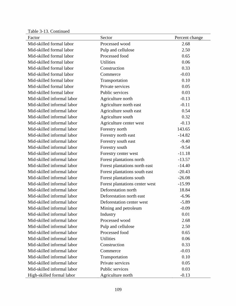
109
Table 3-13. Continued Factor Sector Percent change Mid-skilled formal labor Processed wood 2.68 Mid-skilled formal labor Pulp and cellulose 2.50 Mid-skilled formal labor Processed food 0.65 Mid-skilled formal labor Utilities 0.06 Mid-skilled formal labor Construction 0.33 Mid-skilled formal labor Commerce -0.03 Mid-skilled formal labor Transportation 0.10 Mid-skilled formal labor Private services 0.05 Mid-skilled formal labor Public services 0.03 Mid-skilled informal labor Agriculture north -0.13 Mid-skilled informal labor Agriculture north east -0.11 Mid-skilled informal labor Agriculture south east 0.54 Mid-skilled informal labor Agriculture south 0.32 Mid-skilled informal labor Agriculture center west -0.13 Mid-skilled informal labor Forestry north 143.65 Mid-skilled informal labor Forestry north east -14.82 Mid-skilled informal labor Forestry south east -9.40 Mid-skilled informal labor Forestry south -9.54 Mid-skilled informal labor Forestry center west -11.18 Mid-skilled informal labor Forest plantations north -13.57 Mid-skilled informal labor Forest plantations north east -14.40 Mid-skilled informal labor Forest plantations south east -20.43 Mid-skilled informal labor Forest plantations south -26.08 Mid-skilled informal labor Forest plantations center west -15.99 Mid-skilled informal labor Deforestation north 18.84 Mid-skilled informal labor Deforestation north east -6.96 Mid-skilled informal labor Deforestation center west -5.89 Mid-skilled informal labor Mining and petroleum -0.09 Mid-skilled informal labor Industry 0.01 Mid-skilled informal labor Processed wood 2.68 Mid-skilled informal labor Pulp and cellulose 2.50 Mid-skilled informal labor Processed food 0.65 Mid-skilled informal labor Utilities 0.06 Mid-skilled informal labor Construction 0.33 Mid-skilled informal labor Commerce -0.03 Mid-skilled informal labor Transportation 0.10 Mid-skilled informal labor Private services 0.05 Mid-skilled informal labor Public services 0.03 High-skilled formal labor Agriculture north -0.13
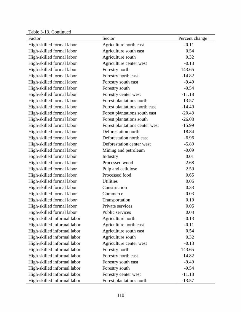
110
Table 3-13. Continued Factor Sector Percent change High-skilled formal labor Agriculture north east -0.11 High-skilled formal labor Agriculture south east 0.54 High-skilled formal labor Agriculture south 0.32 High-skilled formal labor Agriculture center west -0.13 High-skilled formal labor Forestry north 143.65 High-skilled formal labor Forestry north east -14.82 High-skilled formal labor Forestry south east -9.40 High-skilled formal labor Forestry south -9.54 High-skilled formal labor Forestry center west -11.18 High-skilled formal labor Forest plantations north -13.57 High-skilled formal labor Forest plantations north east -14.40 High-skilled formal labor Forest plantations south east -20.43 High-skilled formal labor Forest plantations south -26.08 High-skilled formal labor Forest plantations center west -15.99 High-skilled formal labor Deforestation north 18.84 High-skilled formal labor Deforestation north east -6.96 High-skilled formal labor Deforestation center west -5.89 High-skilled formal labor Mining and petroleum -0.09 High-skilled formal labor Industry 0.01 High-skilled formal labor Processed wood 2.68 High-skilled formal labor Pulp and cellulose 2.50 High-skilled formal labor Processed food 0.65 High-skilled formal labor Utilities 0.06 High-skilled formal labor Construction 0.33 High-skilled formal labor Commerce -0.03 High-skilled formal labor Transportation 0.10 High-skilled formal labor Private services 0.05 High-skilled formal labor Public services 0.03 High-skilled informal labor Agriculture north -0.13 High-skilled informal labor Agriculture north east -0.11 High-skilled informal labor Agriculture south east 0.54 High-skilled informal labor Agriculture south 0.32 High-skilled informal labor Agriculture center west -0.13 High-skilled informal labor Forestry north 143.65 High-skilled informal labor Forestry north east -14.82 High-skilled informal labor Forestry south east -9.40 High-skilled informal labor Forestry south -9.54 High-skilled informal labor Forestry center west -11.18 High-skilled informal labor Forest plantations north -13.57

111
Table 3-13. Continued Factor Sector Percent change High-skilled informal labor Forest plantations north east -14.40 High-skilled informal labor Forest plantations south east -20.43 High-skilled informal labor Forest plantations south -26.08 High-skilled informal labor Forest plantations center west -15.99 High-skilled informal labor Deforestation north 18.84 High-skilled informal labor Deforestation north east -6.96 High-skilled informal labor Deforestation center west -5.89 High-skilled informal labor Mining and petroleum -0.09 High-skilled informal labor Industry 0.01 High-skilled informal labor Processed wood 2.68 High-skilled informal labor Pulp and cellulose 2.50 High-skilled informal labor Processed food 0.65 High-skilled informal labor Utilities 0.06 High-skilled informal labor Construction 0.33 High-skilled informal labor Commerce -0.03 High-skilled informal labor Transportation 0.10 High-skilled informal labor Private services 0.05 High-skilled informal labor Public services 0.03 Capital Agriculture north -0.13 Capital Agriculture north east -0.11 Capital Agriculture south east 0.54 Capital Agriculture south 0.32 Capital Agriculture center west -0.13 Capital Forestry north 143.65 Capital Forestry north east -14.82 Capital Forestry south east -9.40 Capital Forestry south -9.54 Capital Forestry center west -11.18 Capital Forest plantations north -13.57 Capital Forest plantations north east -14.40 Capital Forest plantations south east -20.43 Capital Forest plantations south -26.08 Capital Forest plantations center west -15.99 Capital Deforestation north 18.84 Capital Deforestation north east -6.96 Capital Deforestation center west -5.89 Capital Mining and petroleum -0.09 Capital Industry 0.01 Capital Processed wood 2.68

112
Table 3-13 Continued Factor Sector Percent change Capital Pulp and cellulose 2.50 Capital Processed food 0.65 Capital Utilities 0.06 Capital Construction 0.33 Capital Commerce -0.03 Capital Transportation 0.10 Capital Private services 0.05 Capital Public services 0.03 Agricultural land north Agriculture north -0.17 Agricultural land north Forest plantations north -0.17 Agricultural land north east Agriculture north east -0.38 Agricultural land north east Forest plantations north east -0.38 Agricultural land south east Agriculture south east -6.79 Agricultural land south east Forest plantations south east -6.79 Agricultural land south Agriculture south -1.81 Agricultural land south Forest plantations south -1.81 Agricultural land center west Agriculture center west -0.17 Agricultural land center west Forest plantations center west -0.17 Forestland north Forestry north -64.47 Forestland north Deforestation north -64.47 Forestland north east Forestry north east -14.25 Forestland north east Deforestation north east -14.25 Forestland southeast Forestry south east -9.40 Forestland south Forestry south -9.54 Forestland center west Forestry center west -11.14 Forestland center west Deforestation center west -11.14

113
Table 3-14. Percent change in level of domestic activity Sector Percent change Agriculture north 0.00 Agriculture north east 0.01 Agriculture south east 0.19 Agriculture south 0.13 Agriculture center west 0.01 Forestry north 24.68 Forestry north east -0.02 Forestry south east 0.00 Forestry south 0.00 Forestry center west -0.01 Forest plantations north -0.56 Forest plantations north east -0.62 Forest plantations south east -2.40 Forest plantations south -3.71 Forest plantations center west -1.29 Deforestation north 1.20 Deforestation north east 0.14 Deforestation center west 0.09 Mining and petroleum 0.00 Industry 0.00 Wood processing 0.00 Pulp and paper 0.00 Food processing 0.00 Utilities 0.00 Construction 0.00 Commerce 0.00 Transportation 0.00 Private services 0.00 Public services 0.00

114
Table 3-15. Percent change in quantity of factor demand by sector Sector Factor Percent change Agriculture north Agricultural land north 0.01 Forest plantations north -2.84 Agriculture north east Agricultural land north east 0.06 Forest plantations north east -2.99 Agriculture south east Agricultural land south east 1.83 Forest plantations south east -3.11 Agriculture south Agricultural land south 0.52 Forest plantations south -5.52 Agriculture center west Agricultural land center west 0.01 Forest plantations center west -3.39 Forestry north Forest land north 46.97 Deforestation north 6.22 Forestry north east Forest land north east -0.13 Deforestation north east 0.41 Forestry south east Forest land south east 0.00 Forestry south Forest land south 0.00 Forestry center west Forest land center west -0.01 Deforestation center west 0.29
Table 3-16. Percent change in quantity of domestic sales and exports Good or service Percent change domestic sales Percent change exports Agriculture 0.05 0.31 Forestry 1.95 14.55 Deforestation 0.84 0.00 Mining and petroleum 0.00 0.00 Industrial 0.01 -0.04 Processed wood 0.00 0.00 Pulp and cellulose 0.00 0.00 Processed food 0.02 -0.07 Utilities 0.00 0.00 Construction 0.00 -0.09 Commerce 0.00 0.00 Transportation 0.00 -0.08 Private services 0.00 -0.04 Public services 0.00 0.00

115
Table 3-17. Percent change in quantity of composite goods supply Sector Percent change Agriculture 0.03 Forestry 0.37 Deforestation 0.84 Mining and petroleum 0.00 Industrial 0.01 Processed wood 0.00 Pulp and cellulose 0.00 Processed food 0.02 Utilities 0.00 Construction 0.00 Commerce 0.00 Transportation 0.00 Private services 0.01 Public services 0.00

116
CHAPTER 4 RECURSIVE DYNAMIC COMPUTABLE GENERAL EQUILIBRIUM MODEL WITH
ILLEGAL LOGGING AND DEFORESTATION
Introduction
The static CGE model evaluated the policy impact of forest concessions in the absence of
illegality. Given the economic importance of illegality in the Brazilian forestry sector (56% of
forest sector output in 2003), in order to more realistically and fully evaluate the potential socio-
economic and environmental impacts of forest concessions, the analysis conducted herein
disaggregates and models illegal forestry and illegal deforestation sectors. To enable the
updating of agricultural land stocks resulting from deforestation and to consider the medium-
term implications of the forest concessions policy, a recursive dynamic computable general
equilibrium modeling framework is developed and employed.
Following this introduction, illegal logging is defined and its key causes and effects are
summarized1. Next, illegal logging in Brazil is discussed and estimates of its magnitude and
level of prosecution are provided. Treatment of illegality in CGE models is then reviewed.
Following this review, dynamics in CGE models are introduced. Next, the recursive dynamic
extension to the IFPRI Standard CGE Model in GAMs is presented. The experimental design of
the modeling exercise is developed and is followed by simulation results. The chapter concludes
with a discussion of the key findings.
Illegal Logging
Illegal logging can be characterized as consisting of illegal logging activities, the illegal
movement of forest products, and the evasion of taxes and forestry related payments. Following
Callister (1999, p. 7), illegal logging activities include logging without authorization on public or
private land, logging in breach of contractual obligations, logging that does not respect forestry
law, and the illegal attainment of timber harvest rights. The illegal transport of forest products

117
includes the import and export of tree species protected or banned under national and
international law, the unauthorized transport of specified amounts of timber across within-
country and between-country borders, and the illegal transportation of logs from the forest to the
market. The evasion of taxes and other forest-related payments includes the evasion of fees and
duties through incorrectly reporting timber grades and dimensions, the evasion of license fees,
royalties, taxes and other government fees, and false declarations of input and output costs
(Callister, 1999, p. 8). In this chapter, illegal logging is defined similarly to Callister (1999) with
the exception that the illegal import and export of timber across international borders is not
considered.
Corruption is a special form of illegality; it is closely linked with illegal logging since
each facilitates the presence of the other (Amacher, 2006, p. 86). Corruption involves engaging
public officials and involves public property or power; it is conducted for private gain and is
intentional and clandestine (Contreras-Hermosilla, 2002, p. 9). Corruption enables illegal logging
to take place or allows it to continue without consequence.
Numerous reasons for the presence of illegality in the forest sector are cited in the
literature. The Food and Agriculture Organization (FAO, 2005) reports 5 root causes of forest
sector illegality, namely: flawed policies and legal frameworks, low enforcement capacity,
insufficient data on the characteristics of the forest resource and illegal activities, corruption, and
high demand for timber.
The legal framework for forestry can create incentives for illegal operations when laws
are unrealistic and their implementation and enforcement are not supported by sufficient human
and financial resources (FAO, 2005, p. 7). Laws that are too complex or burdensome can create a
significant barrier for producers’ legal compliance, particularly in the case of producers of a

118
smaller stature. Often these frameworks were developed with little public and industry
participation (FAO, 2005, p. 7). Where governments have low implementation and enforcement
capacity, particularly in highly regulated environments, incentives are created for producers to
engage in illegal activities given the low probabilities of detection and subsequent punishment
(FAO, 2005, p. 9). A lack of information on the forest resource in question and its potential
remoteness render monitoring, detection, and enforcement difficult (FAO, 2005, p. 9).
Corruption and a lack of transparency can induce a mutually beneficial relationship between
illegal operators and government officials (FAO, 2005, p. 12). Corruption is bred through faulty
legal frameworks and programs, weak government and non-government institutions, few checks
and balances resulting in low levels of accountability and transparency, and low public sector
wages (FAO, 2005, p. 11). High levels of demand for timber due to excess processing capacity
create incentives for the illegal acquisition of wood (Contreras-Hermosilla, Doornbosch &
Lodge, 2007, p. 21). Furthermore, road building into previously inaccessible areas can
significantly lower the costs of illegal logging in the absence of mechanisms of control and
incentives for sustainable forest management (Contreras-Hermosilla et al., 2007, p. 23).
It is thus reasonable to assume that with the price of illegal and legal wood practically
equal, economic incentives for operating illegally are created. Rational profit maximizing firms
that base decisions on purely economic criteria will choose to engage in illegal logging when the
benefits are greater than the costs, penalties, and associated risks of operating in illegality
(Tacconi, Boscolo & Brack, 2003, p. 8).
Illegal logging results in negative socio-economic and environmental outcomes. Firms
that evade forestry related payments such as royalties are able to produce an identical and
cheaper product compared to those that operate legally. The world price reduction in forest

119
products due to illegal logging is estimated between 7% and 16% (Seneca Creek Associates &
Wood Resources, 2004). Consequently, firms operating legally suffer from reduced profits, are
discouraged from investing in forest management and ultimately may be forced out of business
(Contreras et al., 2007, p. 19). Depressed prices also create perverse incentives for inefficient
harvesting operations (Gutierrez-Velez & MacDicken, 2008, p. 249; Seneca Creek Associates &
Wood Resources, 2004, p. 55). Illegal logging can lead to future forest productivity losses with
firms operating in illegality shirking the higher management standards required by law
(Gutierrez-Velez & MacDicken, 2008, p. 249).
Society as a whole tends to suffer from the effects of illegal logging. The government
loses a potentially important source of revenue and its ability to provide social services is
reduced (Callister, 1999, p. 19). Lost revenue from illegal logging in developing countries is
estimated at over US$15 billion per year (Contreras-Hermosilla et al., 2007, p. 18). For Brazil,
illegal logging costs the state and society upwards of US$1.1 billion per year (Gutierrez-Velez &
MacDicken, 2008, p. 254). Furthermore, a forest’s capacity to produce critical environmental
services is diminished due to inappropriate logging practices, including increased residual
damage and the logging of sensitive areas and protected species.
Finally, illegal operations can have a negative employment effect; legal operations
require minimum salaries and working conditions whereas illegal operations do not (Gutierrez-
Velez & MacDicken, 2008, p. 249). Short-term employment may be created by illegal logging,
however, the boom and bust nature of these operations does not lend to community stability.
Illegal Logging in Brazil
Illegal logging in Brazil is a function of flawed policies and legal frameworks, low
enforcement capacity, insufficient data on the characteristics of the forest resource and illegal
activities, corruption, and high demand for timber as discussed in the previous section. Rhodes,

120
Allen and Callahan (2006, p. 3) argue that illegal logging’s pervasiveness in Brazil is largely due
to the absence of the rule of law where petty corruption prevails. The authors assert that in many
cases, firms once operating legally were forced into illegality due to increasingly uncertain
property rights, a changing policy environment creating new restrictions on forest operations,
and a lack of forestland on which firms may operate legally (Rhodes et al., 2006, p. 3).
Estimates on the extent of illegal logging in Brazil tend to vary considerably. Smeraldi
(2004, p. 39) reports that the classification and analysis of forest harvesting, commerce, and
illegal logging in Brazil began in the early 1990s. A report prepared in 1994 by the
environmental NGO Amigos da Terra reported that all mahogany harvested in the Brazilian
Amazon was harvested illegally. A second paper prepared by the NGO reported that illegal
harvesting activities were advancing on to public forests and conservation areas in 1994. A
confidential government report leaked to the media in 1997 estimated that 80% of all the timber
in the Brazilian market prior to 1997 was harvested illegally (Smeraldi, 2004, p. 40); this figure
has subsequently been cited in numerous publications (Lele, Viana, Veríssimo, Vosti, Perkins &
Husain, 2000, p. 20; Marquesini & Edwards, 2001, p. 1; Tacconi et al., 2003, p. 8). Seneca Creek
Associates and Wood Resources International (2004, p. 11) report estimates of between 20-90%
of wood harvested in Brazil is done so illegally. More recently, considering roundwood
consumption and the volume authorized through deforestation authorizations and forest
management plans for 2004, over 43% of the timber volume harvested was done so illegally
(calculation based on Lentini et al., 2005a). This figure includes wood sourced from both
selectively logged and deforested areas.
With the approval of Brazil’s Environmental Crimes Law in 1998 and a supporting
Decree in 1999 (Federal Law 9.606/98 and Federal Decree 3.179/99, respectively), efforts to

121
punish illegal logging have increased dramatically. The number of fines applied since 1999 has
increased substantially, though their collection has remained low. The fine for illegal
deforestation is approximately US$700 per hectare (Barreto, Souza, Noguerón, Anderson &
Salomão, 2006, p. 20) while the fine for illegally transporting wood products ranges from
US$28.50 to US$143.00 per cubic meter (Brito, Barreto and Rothman, 2005, p. 13).
An estimated US$16.2 billion in fines were issued in 2001 which is 8 times the fines
issued in 1997; the percentage of these fines collected was 6% (Macqueen, Grieg-Gran, Lima,
MacGregor, Merry, Prochnick, Scotland, Smeraldi & Young, 2003, p. 54). In 1999, The
Brazilian Institute of the Environment and Natural Resources (IBAMA) collected 14% of the
value of fines owed between 1998 and 1999. Between 2001 and 2004, the total value of fines
issued by IBAMA increased 180% from US$103 million to US$290 million. Only 2% of the
fines issued for environmental crimes during this period were collected, however. During the
same period, the illegal timber harvest reportedly fell from 47% to 43% (Brito & Barreto, 2006,
p. 2).
Brito et al. (2005, p. 13) conducted an analysis of a sample of 55 judicial actions for
forestry violations committed in Pará and filed with the Federal Court of Belém between 2000
and 2003. Of this sample, 98% of the cases involved illegally taking, acquiring, selling, storing,
or transporting wood, firewood, charcoal, and other forest products (art. 46 of the Environmental
Crimes Law). Illegal transport and storage accounted for 48% and 24% of the crimes committed,
respectively (Brito et al., 2005, p. 9) while only 8% of the crimes involved illegal logging (6%)
and deforestation (2%; Brito et al., 2005, p. 10). With regards to fine collection, 9% of the cases
or 2% of the value of the fines assessed were paid. In 2003, the average civil liability in 3 cases

122
was US$0.70 per cubic meter while the average criminal liability was US$45.00 per cubic meter
for an overall average of US$45.70 per cubic meter (Brito et al., 2005, p. 13).
Treatment of Illegal Behavior in Computable General Equilibrium Models
Illegal activities in CGE models have received little attention in the literature. The closest
parallel to modeling illegality has involved distinguishing between formal and informal activities
and labor. Informal sector activities and labor are characterized by firms and individuals that do
not comply with regulations and tax codes. Informality emerges where the government imposes
excessive regulations and taxes and lacks the capacity to enforce them (Loayza, 1997, p. 2).
Alternatively, informality may occur when state officials or interest groups profit from
informality and as such they create a regulatory environment that renders operating in the
informal sector beneficial or unavoidable (Loayza, 1997, p. 3). Costs involved in engaging in the
informal sector include fines and penalties, lack of access to public services, unenforceable
property rights on capital and output, and the inability to enter into legally binding contracts
including access to capital markets and insurance (Loayza, 1997, p. 3).
Kelley (1994) analyzed the macroeconomic implications of informal sectors and informal
labor in Peru considering an increase in government and investment demand, and the impact of
an increase in formal sector wages and informal sector productivity. In this model, a shortage of
formal employment results in a parallel informal sector, employing informal labor and producing
a similar, though imperfectly substitutable good or service. Kelley (1994) characterized informal
sector production as organized around an individual, family, or small group where the producer
receives the net product from production rather than a wage, and pays little or no taxes. Informal
sector production technology is labor intensive to reflect capital scarcity. Output from parallel
formal and informal sectors is aggregated into a composite good; relative prices and imperfect
substitutability between the two similar goods determine output levels. Full labor employment is

123
assumed which is made possible through adjustments in the level of informal employment
(Kelley, 1994, p. 1395).
Gibson (2004) developed a dynamic model with an informal sector to evaluate the long-
run effects of macroeconomic and trade reform policies on growth, distribution, human capital
formation, and poverty (Gibson, 2004, p. 61). In this model, non-traded goods sectors have
parallel informal sectors which serve as an employer of last resort, absorbing surplus labor
during recessions and supplying labor in expansionary periods (Gibson, 2004, p. 62). The price
of informal sector output is determined by the formal sector. The informal sector always operates
at full capacity and as in Kelley (1994), informal sector income is earned by the operator
(Gibson, 2005, p. 65).
Fortin, Marceau and Savard (1997) evaluated the effect of taxation and wage controls in
an economy with informal sectors. The informal sector is distinguished from the formal sector by
technological and organizational factors which are reflected through the scale of the firm, a wage
differential between formal and informal workers, and regulatory evasion. In their model, firms
operating in the informal sector do not comply with minimum wage and tax laws. Informal firms
face the risk of being detected and fined unless they engage in a costly activity to avoid
detection. The authors assume that firms would rather pay a sure cost to avoid the risk of being
detected; this sure cost function is described by an inverted L curve where the cost of detection is
zero until firm size reaches a critical limit and the cost of informality rises to infinity (Fortin et
al., 1997, p. 298).
The Australian Bureau of Agricultural and Resource Economics’ model of Papua New
Guinea incorporated a kidnapping and informal sector in their modeling framework with

124
unskilled labor as the primary input to these sectors. Fines applied to the criminal sector are
treated as production taxes in the model (Levantis & Fairhead, 2004, p. 15).
Dynamics in Computable General Equilibrium Models
Policy makers are often interested in how current decisions will affect future
socioeconomic outcomes. Static models provide an indication of the order of magnitude and
direction of effect of a policy shock and are typically either short-run or long-run depending on
the factor and macroeconomic closures chosen by the modeler. In contrast, dynamic models are
used to simulate the impact of a policy on the economy for a definite time period. The main
advantages of this class of models is their ability to shed light on the economic transition path
resulting from a policy shock and the short-term costs and longer-term gains resulting from
policy implementation (Cattaneo, 1999, p. 17). Furthermore, dynamic models typically involve a
deeper treatment of investment behavior and enable the modeler to update key growth
parameters such as population, labor force, factor productivity, world prices, and government
consumption as well as rates of capital depreciation. Dynamic models are thus a useful tool for
informing policy decisions.
Four main approaches to dynamic modeling may be distinguished. Following Dixon and
Parmenter (1996, p. 24), the distinction between approaches is based on the treatment of
investment and capital accumulation. In the first approach, investment is modeled exogenously
with agent expectations modeled as static. Agents exhibiting static expectations assume no
changes in decision parameters over time. This type of model is recursive dynamic where the
inter-temporal trajectory of the economy is determined by calculating a series of static equilibria
which are related to each other by capital formation processes and exogenous changes in growth
parameters (Pereira & Shoven, 1988, p. 402).

125
The second approach differs from the first in that investment is modeled endogenously
and agent investment behavior is based on adaptive expectations. Agents with adaptive
expectations use information on previous rates of return to capital to inform their current
investment decisions. This class of models is also solved recursively.
Third, investment may be modeled endogenously where agents engage in forward-
looking investment behavior. These agents consider both the present and future to inform their
current investment decisions (Springer, 1999, p. 5). In this case, an agent’s expectations about
expected rates of return to capital for a given year are equal to the actual rates of return for that
year. Differing from recursive dynamic models, this class of models is solved simultaneously for
all time periods.
In the final case, investment behavior is optimized and modeled as an inter-temporal
decision where inter-temporal substitution possibilities exist (Dixon & Parmenter, 1996, p. 25-
36; Springer, 1999, p. 6). This class of models is also solved simultaneously for all time periods.
Since perfect foresight is not generally representative of how investment behaves in the
real world, the model in the next section follows the second approach, where investment
behavior is based on adaptive expectations and the model is solved recursively.
Dynamic Extension to the Standard Computable General Equilibrium Model in GAMS
The Recursive Dynamic Computable General Equilibrium Model is a dynamic extension
to the IFPRI Standard CGE Model in GAMS and was developed by Robinson and Thurlow (no
date). The within period (year) specification of the model is identical to that of the Standard
IFPRI model described in Chapter 3. The between period specification contains adjustments to
account for endogenous investment, and exogenous population and labor force growth,
depreciation, and changes in total factor productivity (Robinson & Thurlow, no date, p. 1). The
sectoral allocation of capital is modeled as a function of the rate of capital depreciation and the

126
differential in profits between sectors from the previous period (Thurlow, 2004, p. 11).
Endogenous adjustments to account for capital accumulation and exogenous adjustments to
population, labor force and total factor productivity are discussed in turn.
Capital supply is based on the previous period’s capital stock and allocation of
investment spending. Investment is carried out in proportion to a sector’s share in economy-wide
capital income and is adjusted by the ratio of a sector’s rate of profits and the economy-wide
average rate of profit. This specification implies that a sector with higher than average profits
will receive a larger share of investment than its average share in aggregate capital income
(Robinson & Thurlow, no date, p. 4; see Appendix A, equations 50 to 54).
Population growth has a direct and positive impact on household consumption
expenditure with the quantity of income-independent consumption increasing at the same rate as
population growth (Robinson & Thurlow, no date, p. 2). The level of minimum household
consumption expenditure also increases proportionally with population growth. Growth affects
average rather than marginal consumption demand implying that new consumers share the same
preferences as existing consumers (Robinson & Thurlow, no date, p. 3). The parameter , the
subsistence consumption of marketed commodity c for household h, and 'hac hγ , the subsistence
consumption of home commodity c from activity a for household h, are both adjusted upwards
by the rate of population growth (see Appendix A).
With regards to labor force growth, with a fixed labor supply, flexible nominal wages and
full employment, the between period levels of labor supply are adjusted according to the rate of
labor force growth (Robinson & Thurlow, no date, p. 4; see Appendix A). The parameter fQFS ,
the quantity of factor supply, is adjusted upwards by the rate of labor force growth.
mchγ

127
Changes in total factor productivity are imposed exogenously by introducing a
technological parameter in the model equations for the calculation of the quantity of aggregate
value-added (Robinson & Thurlow, no date, p. 6; see Appendix A). The parameter vaaα , the
efficiency parameter in the Constant Elasticity of Substitution value-added function, is adjusted
upwards by total factor productivity growth.
The dynamic extension to the Standard CGE Model in GAMS is programmed and solved
as a mixed complementarity problem using the General Algebraic Modeling System and the
PATH solver.
Customizing the 2003 Social Accounting Matrix for Brazil to Describe Illegal Forestry and Illegal Deforestation
Illegal forestry and illegal deforestation activities are not explicitly described in the
national accounts data from which the SAM for Brazil was constructed. Expenditures and
receipts from these activities are aggregated with those of the legal forestry sector, however,
since once timber is extracted from the forest, it is presented to consumers as a legal product and
accounted for as such. Therefore, in customizing the SAM to describe illegal forestry and illegal
deforestation activities, expenditures are disaggregated from the legal forestry sector (with two
exceptions noted below). The following subsections describe the procedures used in
disaggregating illegal forestry and illegal deforestation in the Brazilian SAM and provide a
summary of the key assumptions made.
Illegal Deforestation
The starting point for disaggregating the illegal deforestation sector in the SAM is to
estimate the total area illegally deforested in 2003. Illegal deforestation in this analysis is defined
as the removal of timber and the subsequent clearing of forests in the absence of a valid
deforestation authorization and the illegal transport of timber from the forest to the mill. As with

128
the legal deforestation considered in Chapter 3, illegal deforestation occurs in Brazil’s north,
north east and center west regions.
Total deforestation in Brazil’s Legal Amazon in 2003 was 2,528,200 hectares (The
National Institute for Space Research’s [INPE] Program for the Calculation of Deforestation in
Amazonia [PRODES]). Deducting legally authorized deforestation registered with Brazil’s
monitoring and control system for resources and forest products database (SISPROF; 210,032
Ha), illegal deforestation in 2003 was approximately 2,318,168 hectares (MMA, 2008a).
Forest product output from illegal deforestation is calculated next. It is reasonable to
assume that only timber harvested in proximity to new logging centers can be fully utilized since
the difficult access and the state’s reduced monitoring and enforcement capabilities decrease the
probability that illegality will be detected and penalized (Lentini, 2008, personal
communication)2. Therefore, it is assumed that illegal deforestation produces the same amount of
timber per unit area as legal deforestation only in proximity to new logging centers. To calculate
the area deforested in proximity to these centers, levels of deforestation by municipality were
obtained from the PRODES online server while the location of new logging centers was
extracted from Lentini et al. (2005a, p. 63). Illegal deforestation in municipalities in which new
logging centers are located amounted to 15.7% and 27.1% of total illegal deforestation in the
north and center west, respectively. Therefore, illegal deforestation produces 15.7% and 27.1%
of the timber that the legal deforestation sector produces per unit area in the north and center
west, respectively3. Given the lack of data on logging centers in the north east and its easier
access, it is assumed that illegal deforestation in this region produces 10% of the timber per unit
area when compared with legal deforestation.

129
The illegal deforestation sector’s expenditures on intermediate consumption, labor and
capital for producing forest products is identical to that of the legal deforestation sector’s
expenditure per unit area. These expenditures, along with the value of the illegal deforestation
sector’s forest product output value are deducted from the legal forestry sector.
The treatment of the illegal deforestation sector’s expenditure on forestland and its
payments to the indirect tax account differs from that of the legal deforestation sector’s
expenditures and payments. First, with regards to forestland, it is assumed that illegal
deforestation operations occurring on 50% of Special Areas (military zones, quilombola
communities which are areas settled by the descendents of slaves, Environmental Protection
Areas, and rural settlements) and on private land in dispute and terra devoluta make reduced
forestland payments. This is a reasonable assumption since, private land aside, most illegality
occurs on land with these tenure types. Furthermore, it is assumed that these illegal operations
pay 75% of the legal deforestation sector’s forestland rent per unit of output. The rationale for
this reduced payment is that firms that acquire land illegally are assumed to pay less than those
that do so legally due to weaker property rights guarantees and the risks inherent in the illegal
acquisition of land. To calculate the percentage reduction in forestland payments, the total area in
Special Areas, private land, private land in dispute, and terra devoluta is calculated based on
IBGE data (1996; cited in Lentini et al., 2005a, p. 32). Based on this value, the proportion of area
in 50% of Special Areas, private land in dispute, and terra devoluta is calculated and represents
the proportion of production that is subject to reduced forestland payments (0.76, 0.57 and 0.34
in the north, north east and center west, respectively). These proportions are multiplied by 0.75
and each region’s legal forest sector payment to forestland for a given unit of forest product

130
output to determine the illegal sector’s forestland payment per unit of forest product output by
region4.
With regards to activity taxes, the illegal deforestation sector does not pay activity taxes.
Illegal deforestation operations are, however, subject to fines if their illegal activities are
detected and they are successfully prosecuted. It is therefore necessary to estimate the value of
fines issued in 2003 as well as the collection rate for the same year. The value of fines issued to
the illegal sectors is extrapolated from IBAMA and Macqueen et al. (2003, p. 54) data. Based on
estimates from Macqueen et al. (2003, p. 54), Brito et al. (2005, p. 10), Brito and Barreto (2006,
p. 3), and IBAMA data, a conservative estimate of 6% of the rate of collection for fines issued is
made and applied to the estimate of the value of fines issued. The value of fines paid by region is
distributed according to the weight of the value of each region’s illegal output of forest products.
Under the balanced macroeconomic closure used in the modeling experiments to follow,
government savings are flexible and tax rates are fixed (i.e. the activity tax or fine is treated as a
fixed share parameter and is calibrated from the SAM). Treating the fine as a fixed share implies
that as an illegal sector’s output increases, so does the amount of the fine that it pays.
Next, the additional expenditures on labor for clearing forestland are accounted for. From
Cattaneo (2002), clearing one hectare of forestland requires half a month of low-skilled labor.
The cost of labor for forest clearing is thus the product of half of the average monthly wage for
the forestry sector and the forest area cleared. The imbalance in expenditure on labor which is
generated as a result of this additional labor payment is distributed among all sectors in
accordance with the weight of each sector’s labor expenditure. The imbalance created in the
indirect tax account resulting from the illegal sector’s payment of fines is distributed among all
sectors according to the weight of each sector’s indirect tax expenditure.

131
The difference between the illegal deforestation sector and the legal deforestation sector’s
expenditure to produce a unit of output is referred to as the deforestation product in the SAM.
This is considered to be the level of above normal profits earned for operating illegally and is
allocated according to an assumption matrix which describes how these profits are distributed to
each labor class.
Finally, adjustments to the SAM are made to account for the consumption of the
deforestation product. With the disaggregation of the illegal deforestation sector, the size of the
deforestation product is larger than when only legal deforestation was considered. The sole
consumer of the deforestation product is the deforestation institution. This institution derives all
of its income from the returns to agricultural land. To provide the additional income that the
deforestation institution requires to consume the deforestation product, the value of the
deforestation product is deducted from the total agricultural land rent distributed to households
and enterprises. This amount is deducted according to the weight of each institution’s share of
agricultural land rent and is then reallocated as income to the deforestation institution.
Illegal Forestry
The starting point for disaggregating an illegal forestry sector in the SAM is to calculate
the Legal Amazon’s total illegal forest product output. First, the total volume of timber
authorized through forest management plans and deforestation authorizations in 2003 is
calculated. Next, total roundwood consumption for 2003 is extrapolated from data for 1998 and
2004 (Lentini et al, 2005a, p. 69; Lentini et al., 2005b, p. 1). The authorized volume is deducted
from total consumption revealing that the illegal harvest volume from illegal deforestation and
illegal forestry was 56% of total output in 2003. The difference between total illegal forest
product output and the illegal deforestation sector’s forest product output is the illegal forestry
sector’s output.

132
The illegal forestry sector’s expenditures on intermediate consumption, labor and capital
are assumed to be the same as that of the legal forestry sector’s expenditures per unit of output.
These expenditures are deducted from the legal forestry sector’s expenditures. The illegal
forestry sector’s payments to forestland and its payments of fines are calculated in the same way
as for the illegal deforestation sector. Since the illegal sector generally pays less forestland rent
and makes smaller payments to the indirect tax account (interpreted as fines), the illegal sector’s
expenditure for a given unit of output is less than that of the legal sector. As in the case of the
illegal deforestation sector, this difference is interpreted as above normal profits and is
distributed to labor in the same manner as in the case of the illegal deforestation sector.
Summary of Key Assumptions
1. Illegal deforestation produces less timber per unit area than the legal deforestation sector.
2. The illegal deforestation and illegal forestry sectors pay less for forestland per unit of forest product output than their legal counterparts.
3. The illegal deforestation and illegal forestry sectors do not pay activity taxes rather they pay fines based on the amount of fines and the collection rate estimated for 2003.
4. The deforestation institution derives all of its income from the returns to agricultural land which enables it to finance the production of forest products and the clearing of forestland.
5. The difference between an illegal and legal sector’s (for both forestry and deforestation) expenditure to produce a unit of forest product output is considered to be the level of above normal profits earned for operating illegally; this profit is allocated to labor.
Scenario Design
Two scenarios are simulated in this chapter. The baseline scenario projects the Brazilian
economy from the base year of 2003 to 2018 in the absence of forest concessions. The policy
shock scenario uses the results of the base year projection and simulates the establishment of
forest concessions in the Brazilian Amazon from 2008 to 2018. The difference between the

133
baseline and policy shock scenarios is the policy impact of forest concessions on the Brazilian
economy. This section develops the baseline and policy shock scenarios in detail.
In contrast to the static CGE model of Chapter 3, the recursive dynamic model enables
the updating of factor stocks. In both the baseline and the policy shock scenarios, labor supply is
updated based on the estimated labor force growth rate. Capital stocks are updated endogenously
based on the previous period’s allocation of investment and the rate of capital depreciation5. In
both the baseline scenario and the policy shock scenarios, the stock of agricultural land is also
updated each year. Since the legal and illegal deforestation sectors clear forestland, the quantity
of forestland cleared in one year is used to update the factor supply of agricultural land in the
subsequent year and is thus made available to the agricultural and forest plantations sectors6.
Figure 4-1 represents the relationship between natural forest management, forest plantations,
agriculture, forestland, and agricultural land. Equation 4-1 demonstrates the updating of the
agricultural land stock based on the previous period’s level of deforestation using the stock of
agricultural land in the north as an example.
, , , , , ,
, , 4-1 Where:
, , = Quantity of factor f demanded by activity a in time t.
, , = Quantity of factor supply for activity a in time t.
In the policy shock scenario, the forest concessions policy is simulated as an increase in
the factor supply of forestland in the north. Of the 193.8 million hectares of public forests
registered in Brazil’s National Registry of Public Forests, 43.7 million hectares (22.5%) are
legally eligible to be designated as forest concessions; 99.8% of these forests are located in the

134
Legal Amazon. Of this area, 11.6 million hectares may be designated as Management Units for
forest concessions for the 2007 to 2008 period, over 99% of which are located in Brazil’s
northern administrative region (i.e. in the Legal Amazon with the exception of the state of Mato
Grosso). The state of Pará alone accounts for over 82% of this area. The majority of these forests
are National Forests with approved forest management plans or National Forests with
management plans that are in the process of development. Of the 11.6 million hectares of forest,
3.9 million hectares were designated as priority areas for forest concessions, all of which are
located in the states of Pará and Rondônia. One million hectares of this area in 2008 are expected
to be designated as Management Units and put up for bidding as forest concessions (SFB, 2007,
p. 30). Over the next 10 years, the maximum area that the state plans to designate as forest
concessions is 13 million hectares or 3% of Amazônia (MMA, 2005, p. 5). Taking a more
conservative estimate of 10 million hectares over the next 10 years, the policy scenario
introduces 1 million hectares of forestland stock per year in the north beginning in 2008, with the
final 1 million hectares introduced in 20177.
A mathematical formulation of this addition of forestland is as follows. The sum of all
activities’ demand for a given factor is equal to the total factor supply as given by equation 4-2.
For simplicity, the element of time is dropped.
∑ , 4-2 Where:
, = Quantity of factor f demanded by activity a. = Quantity of factor supply.
0 = Initial quantity of factor supply.

135
As an example, in the first year of forest concessions implementation, forestland supply
is increased by 46% in the north. Given equation 4-3, this increase enters the model as in
equation 4-4.
Since:
0 4-3
1.46 · 0 4-4
Illegal forestry operations produce less timber and generate more wood waste than their
legal counterparts. Following Gutierrez-Velez and MacDicken (2008, p. 252), planned logging is
used as a proxy for legal forestry and unplanned logging is used as a proxy for illegal forestry.
Barreto, Amaral, Vidal and Uhl (1998, p. 13) found that planned forestry operations harvest 30%
more timber than unplanned operations due to less waste during felling and skidding. To account
for inefficiencies in illegal operations as well as the increasing scarcity of forestland available for
use by the illegal logging and illegal deforestation sectors in the north, a yield distortion
parameter is introduced into the illegal forestry and illegal deforestation sectors’ equations for
forest and deforestation product output per unit of activity. Equation 4-5 is a mathematical
representation of the impact of the distortion parameter on a sector’s activity level. In this
equation, as a sector’s activity level increases, its output increases at a slower rate as determined
by the yield distortion parameter.
∑ · · 4-5 Where:
= Quantity of household home consumption of commodity c from activity a for household h.
= Quantity of marketed output of commodity c from activity a.
= Yield distortion parameter for activity a and

136
commodity c. = Yield of output of c per unit of activity a. = Activity level.
In order to calculate the distortion parameter, the area of forest concessions established
each year is deducted from the total federal public forests eligible for forest concessions. The
proportion of the value calculated above and the total federal public forests eligible for forest
concessions is calculated and is interpreted as the distortion parameter. With 1 million hectares
of public forests designated as forest concessions per year, this distortion parameter is smaller in
value and larger in effect year upon year8.
With regards to model closure rules, in both the baseline and policy shock scenarios, the
modeling experiment is run in a balanced macroeconomic environment where investment and
government consumption shares are fixed while the quantities are flexible. Nominal absorption
shares of investment and government consumption are fixed at their base year levels. With
regards to factor closures in the baseline and policy shock scenarios, labor, capital, agricultural
land, and forestland are fully employed and mobile between sectors. A flexible real exchange
rate is chosen for the rest of the world closure while the government closure fixes direct tax rates
enabling flexible government savings. The domestic price index is chosen as the numeraire.
Results
Changes in macroeconomic indicators in the baseline scenario are presented in Table 4-1.
The annual compound percent change (ACPC) in real GDP at market prices is 5.5%. The annual
ACPC in household consumption, investment, government consumption, exports, and imports
are 5.9%, 6.2%, 4.4%, 5.1%, and 5.8%, respectively. Slight deflationary pressure is reflected in
the ACPC of the consumer price index (-0.2%). There is a reduction in private savings as a
percentage of GDP (-0.6%) which is compensated for by an increase in government savings

137
(0.6%). There is an increase in the ACPC in low-income, mid-income and high-income
households’ consumption (3.7%, 5.6% and 6.6%, respectively). The welfare of all households
improves; the ACPC in equivalent variation is 5%, 8.6% and 11.2% for low, mid and high-
income households, respectively.
The impact of the forest concessions policy on the economy is calculated as the
difference between the value of indicators in the baseline scenario and the policy shock scenario.
The policy impact on real GDP at market prices is positive for all years with the exception of
2009 (Figure 4-2). The policy impact on other macroeconomic indicators is small with the
exception of the deforestation institution’s consumption and welfare (Table 4-1). This
institution’s consumption in the baseline grows at 3.3%; it decreases with the concessions policy
scenario at a rate of -9.2% per annum for a difference of -12.5%. Equivalent variation in the
baseline grows at 17.3% and decreases by -3.0% in the policy scenario for a yearly average
difference of -20.3%.
A large and positive impact on activity levels is experienced by the legal and illegal
forestry sectors in the north (Figure 4-3). The policy has a small negative impact on legal
forestry in the north east, south east and south, and on illegal forestry in the north east. There is a
small positive effect on the legal and illegal forestry sectors in the center west. Forest
concessions have a large positive impact on the average annual growth rate (AAGR) of legal
forestry activity in the north and center west while they have a negative effect on the AAGR of
activity levels in the north east, south east and south (13.53%, 4.09%, -2.22%, -0.08% and -
0.04%, respectively; Table 4-2). The impact on illegal forestry’s AAGR in activity is positive
and the highest in the north and center west and negative in the north east (10.59%, 2.93% and -
2.78%, respectively).

138
With regards to policy impacts on legal deforestation activity levels, there is a positive
effect, the largest of which occurs in the north, followed by the center west and north east
(Figure 4-4). The policy has a very small negative impact on illegal deforestation in the north
east and a large negative impact in the north, followed by the center west. The policy has a large
and positive effect on the AAGR of legal deforestation’s activity level; the effect is the greatest
in the center west, followed by the north east and north (10.22%, 9.92% and 8.74%, respectively;
Table 4-2). Illegal deforestation’s AAGR in activity is negatively impacted, most dramatically in
the north, followed by the north east and center west (-26.08%, -7.47% and -5.19%,
respectively).
The policy impact on forest plantation activity is negative and the largest in the south,
followed by the north east, north, center west and south east (Figure 4-5). The policy negatively
affects the AAGR of the forest plantations sector’s activity, with the largest effect in the center
west followed by the north, north east, south and south east (-3.28%, -3.11%, -2.65%, -2.56%
and -1.87%, respectively; Table 4-2).
There is a large positive effect on pulp and cellulose and wood processing activities
(Figure 4-6). The processed wood and pulp and cellulose AAGR in activity levels is positively
impacted (0.38% and 0.75%, respectively; Table 4-2).
The forest concessions policy has a relatively large and positive impact on agricultural
activity in all regions but the center west (Figure 4-7). The impact on the AAGR of agricultural
activity levels is also positive in the north, north east, south east and south, and negative in the
center west (0.45%, 0.36%, 0.09%, 0.18% and -0.05%, respectively; Table 4-2).
The policy impact on composite commodity supply for agricultural and forest products,
processed wood, and pulp and cellulose is positive and most pronounced for agricultural product

139
supply (Figure 4-8). The effect on the AAGR in composite commodity supply is positive for
agricultural and forestry products, processed wood, and pulp and cellulose (0.09%, 0.47%,
0.14% and 0.76%, respectively; Table 4-3); the supply of all other goods and services is also
positively impacted with the exception of commercial services.
Figure 4-9 reveals that the policy has a considerable positive impact on domestic demand
for agricultural and forestry products. Domestic demand for processed wood and pulp and
cellulose, and export demand for agricultural and forest products also increase. The AAGR for
domestic demand of agricultural and forestry products, processed wood, and pulp and cellulose
increases by 0.10%, 1.10%, 0.15% and 0.76%, respectively; the AAGR in exports increases by
0.21%, 2.53%, 0.86% and 0.74% for agricultural and forestry products, processed wood, and
pulp and cellulose, respectively (Table 4-4).
With regards to composite commodity prices, the forest concession policy has a large
negative impact on forest product prices, a smaller negative impact on processed wood and
agricultural product prices, and a negligible effect on pulp and cellulose prices (Figure 4-10).
The policy impact on the AAGR for agricultural and forest products prices, processed wood, and
pulp and cellulose is -0.09%, -0.94%, -0.32% and 0.00%, respectively (Table 4-5).
Figure 4-11 and 4-12 depict the policy impact on the stock of agricultural land and
forestland in the north, north east and center west. The policy impact is positive for agricultural
land stocks in the north and the north east as a result of deforestation and negative in the center
west. Forestland stock in the north increases beginning in 2008 as forest concessions are
established.
The policy impact on the legal deforestation sector’s demand for forestland in the north
east is positive and pronounced after 2008 and remains relatively constant thereafter (Figure 4-

140
13); the effect on the illegal and legal forestry sectors’ demand is negative. There is a small
negative effect on the illegal deforestation sector’s demand for forestland in the north east; there
is no policy impact on demand in the south and south east. In the north east, the AAGR of legal
deforestation’s demand for forestland increases while legal and illegal forestry and illegal
deforestation demand decrease (9.93%, -2.16%, -2.77% and -7.45%, respectively; Table 4-6);
there is no effect on demand in the south and south east.
The legal and illegal forestry sectors’ demand for forestland in the north is positively and
strongly affected by the forest concessions policy, though the latter to a lesser degree (Figure 4-
14). The legal deforestation sector’s demand for forestland in the north is positively impacted by
a small degree while the illegal deforestation sector’s demand is negatively affected. In the
center west, the legal forestry, legal deforestation and illegal forestry sectors’ demand for
forestland is positively affected while the illegal deforestation sector is negatively impacted. The
policy impacts on the AAGR in demand for forestland are positive for legal forestry, illegal
forestry and legal deforestation in the north, while illegal deforestation in the north suffers a
marked negative impact (13.69%, 10.67%, 8.92% and -25.78%, respectively; Table 4-6). The
AAGR of legal forestry, illegal forestry and legal deforestation demand for forestland in the
center west is positively affected while illegal deforestation’s demand is negatively affected
(4.14%, 2.95%, 10.27% and -5.10%, respectively).
Figure 4-15 describes the policy impact on demand for agricultural land in the north east,
south east and south. The agricultural sector’s demand for land in the south is the most positively
affected of these 3 regions, followed by the agricultural sector in the north east and south east.
The forest plantations sector is the most negatively impacted of these 3 regions in the south
followed by the south east and north east. The agricultural sector’s demand for agricultural land

141
in the north is positively impacted to a large degree and negatively affected in the center west
(Figure 4-16). The forest plantation sector’s demand for land is negatively impacted the most in
the center west and then in the north. The effect on the agricultural sector’s AAGR in demand for
agricultural land is positive in the north, north east, south east and south; it is negative in the
center west (0.48%, 0.50%, 0.18%, 0.22% and -0.04%, respectively; Table 4-6). The forest
plantation sector’s AAGR in demand for land is negatively impacted in all regions (-3.06%, -
2.54%, -1.87%, -2.55% and -3.27% in the north, north east, south east, south and center west,
respectively).
The policy impact on household income is depicted in figure 4-17. High-income
household income is the most positively affected, followed by enterprise and mid-income and
low-income household income. From 2009 to 2012 and 2009 to 2010, the policy impact on low-
income and mid-income households, respectively, is negative; the impact on high-income
households is always positive, though the difference between the baseline and the policy shock
also dips slightly in 2009. The AAGR in income increases for low-income, mid-income and
high-income households and the enterprise (0.01%, 0.02%, 0.03% and 0.02%, respectively;
Table 4-7). Policy impacts on household expenditures follow the same trends as those described
for household income (Figure 4-18).
Figure 4-19 describes the policy impact on labor and capital income. Low-skilled labor
income in the policy scenario is less than in the baseline from 2009 to 2016, though the effect
becomes positive after 2016. Mid-skilled and high-skilled labor and capital experience a negative
impact on their income in 2009, though the effect is positive thereafter. The policy impact on the
AAGR for low-skilled, mid-skilled and high-skilled labor, and capital income is positive (0.01%,
0.03%, 0.03% and 0.03%, respectively; Table 4-8).

142
Forestland income in the north increases dramatically with the implementation of forest
concessions (Figure 4-20). Forestland income in other regions changes little in comparison,
though it tends to be generally negatively affected as a result of the policy. The policy impact on
the AAGR in forestland income increases markedly in the north and declines in the north east,
south east, south and center west (5.39%, -0.66%, -1.32%, -1.14% and -2.39%, respectively;
Table 4-8).
In figure 4-21, the policy impact on agricultural land income is depicted. The policy
effect in the north is negative in 2008, positive in 2009, negative from 2010 to 2014, and positive
thereafter. In the north east, the effect is negative in 2008, positive in 2009 and negative in all
subsequent years. In the south east, south and center west, it is negative for all years. The policy
impact on the AAGR in agricultural land income in the north is positive, while it is negative in
the north east, south east, south and center west (0.08%, -0.49%, -0.47%, -0.30% and -0.14%,
respectively; Table 4-8).
Figure 4-22 depicts the policy impact on labor wages and the price of capital. The effect
on low-skilled labor wages is negative and quite pronounced from 2009 to 2016; the effect
becomes positive after 2016. The impact on mid-skilled labor wages is negative only for 2009.
Mid-skilled and high-skilled labor experience a positive impact on their wages as a result of the
policy while the price of capital is positively affected to a much lesser degree. The impact on the
AAGR in low-skilled, mid-skilled and high-skilled labor wages and the price of capital is
positive (0.01%, 0.03%, 0.03% and 0.02%, respectively; Table 4-9).
The impact on the price of forestland in the north east spikes positively in 2009 and
declines steadily thereafter; the effect is negative in 2008, positive from 2009 to 2014 and
negative thereafter (Figure 4-23). The impact is negative in all other regions with the greatest

143
effect on forestland prices in the north followed by the center west. The policy impact on the
AAGR in forestland prices is negative in all regions (-6.20%, -0.66%, -1.32%, -1.14% and -
2.39% in the north, north east, south east, south and center west, respectively; Table 4-9).
The policy impact on agricultural land prices is negative for all regions (Figure 4-24).
Prices are negatively affected the most in the south east and north east, and less dramatically in
the south and north. Although prices are negatively affected in the center west, this effect is less
pronounced than in other regions. The impact on the AAGR in agricultural land prices is
negative in all regions (-0.36%, -0.78%, -0.47%, -0.30% and -0.07% in the north, north east,
south east, south and center west, respectively; Table 4-9).
Discussion
The baseline model results reveal a 5.5% rate of real GDP growth over the time horizon
(Table 4-1). This figure is a reasonable estimate when compared to other real GDP growth
projections that vary between 4% and 5% (Jaeger, 2006, p. 1; Ministério de Minas e Energia, no
date; Patusco, 2002; Purushothaman, no date; The World Bank, 2008, p. 22).
In the baseline scenario, legal forestry in the north and center west contract while
expanding in all other regions (Table 4-2). With forest concessions implemented in 2008, the
opposite becomes true- the policy impact is positive in the north and center west and negative in
other regions. This is an indication of the current scarcity of forestland for forest management.
The increased availability, however, results in greater growth in the illegal forestry sector in the
north and center west rather than the contraction experienced in the baseline. Illegal forestry
grows at a slower rate than the legal forestry sector given the increasing scarcity of forestland for
illegal activities with the establishment of forest concessions.
With increased activity and output resulting from forest concessions, the policy impact on
the forest plantation sector, although it continues to grow, is negative in all regions (Table 4-2).

144
This result, however, does not take into consideration investments that have already been made
in forest plantations which are yet to bear their full economic impact.
Legal deforestation in the baseline expands in the north and contracts in the north east
and center west. The policy impact, however, leads to positive and faster growth in all regions.
Illegal deforestation grows in the north and center west and contracts in the north east in the
baseline; the policy impact, however, results in a contraction in all regions. This contraction in
illegal deforestation is a function of the increasing scarcity of forestland on which firms may
operate illegally and the reduced returns to agricultural land which fund the deforestation
institution (Table 4-2). In summary, the policy impact of forest concessions on illegality is to
reduce the rate of growth of illegal forestry in the north east and the rate of illegal deforestation
in all regions.
As a result of the forest concessions policy, the rate of agricultural growth increases in all
regions with the exception of a small decrease in the center west. While the greater rate of
expansion in the north and north east are a result of faster rates of legal deforestation and
therefore the production of agricultural land, the decline in the center west appears to be the
result of a relatively large decrease in illegal deforestation, given the importance of this sector in
generating agricultural land.
Various economic indicators such as real GDP, household income, agricultural and forest
product supply and forest plantation activity exhibit a positive or negative spike in 2008 or 2009
as a result of the forest concessions policy. Where these spikes occur in 2008, they are the result
of the increased availability of forestland in the north. Where they occur in 2009, it is reasonable
to assume that this variation is the result of the combined economic impact of greater forestland

145
availability in the north as well as increased scarcity in forestland for illegal activities. These
spikes represent a brief period of economic adjustment to policy implementation.
With a growing population and labor force, it is expected that through time, the domestic
demand for aggregate sectoral output will increase. In the baseline, this is the case with domestic
demand growing between 3% and 6% (Table 4-4). This is also true in the forest concessions
policy scenario where the largest impacts on domestic demand are for forestry and agricultural
products, processed wood, and pulp and cellulose; in the case of exports, the policy impact is
also positive for these products. With regards to composite commodity prices, forestry and
agricultural product as well as processed wood product prices increase in the baseline (Table 4-
5); the policy impact of forest concessions, however, results in a reduced rate of growth in these
prices.
Just as the level of activity of the legal and illegal forestry sectors in the north and center
west are positively affected by the policy, growth in their demand for forestland also increases.
In the case of illegal deforestation in the north and center west, the growth in demand for
forestland is positive in the baseline; the policy, however, results in a negative rate of growth for
this activity’s demand for forestland. In the north east, the policy impact on growth in demand
for forestland is positive although still decreasing.
The policy impact on the rate of growth in the agriculture sector’s demand for
agricultural land increases in all regions but the center west. This increased growth in demand is
met by a reduced rate of growth in the forest plantations sectors’ demand for land and an
increase in the rate of growth of legal deforestation and therefore an increasing stock of
agricultural land.

146
With regards to household income, there is a positive overall policy impact on income
levels (Table 4-7). With high and mid-income households receiving a greater share of income
from deforestation among other things, their incomes also grow at a faster rate. Low-income and
mid-income households experience an adjustment period to the policy shock with their incomes
being negatively affected in comparison to the baseline for 4 and 2 years, respectively; high-
income households are positively affected throughout the simulation period.
Through time, in the baseline, labor and capital income increases; forest concessions have
a positive impact on the income of all labor classes as well as capital (Table 4-8). The policy
impact on growth of forestland income is large and positive in the north and negative in other
regions. With the price of forestland negatively impacted by the policy in all regions (Table 4-9),
the increase in forestland income in the north is explained by the increase in the stock and
demand for forestland in the north. The greatest negative effect on forestland prices is in the
north followed by the center west.
With regards to agricultural land income, the average rate of growth is increasing in the
baseline; in the policy shock scenario, the policy impact is negative in all regions but the north
(Table 4-8). With agriculture in all regions with the exception of the center west exhibiting
greater growth in demand for agricultural land as a result of the policy, the negative impact on
agricultural land income is due to the magnitude of the negative impact of the policy on the price
of agricultural land in all regions (Table 4-9). Interestingly, in the north, the impact on
agricultural land income is negative in 2008 and from 2010 to 2014. This is an indication that the
policy impact on agricultural land income is mixed initially requiring a number of years for
adjustments to take place.

147
1 Although beyond the scope of the current discussion, the drivers of deforestation are reviewed in Kaimowitz & Angelsen (1998); a literature review of the drivers of deforestation may be found in Glantz, Brook &Parisi (1997). 2 New logging centers were established less than 10 years ago (as of 2004) and are located primarily in western Pará and the extreme north west of Mato Grosso (Lentini et al., 2005a, p. 37); these centers form an arc from the BR-163 highway in western Pará to the extreme north west of Mato Grosso until the southern reaches of the state of Amazonas close to the Trans-Amazon highway (Lentini et al., 2005a, p. 62). 3 In the case of the center west, given the high levels of deforestation and the large number of new logging centers, this value is further adjusted downwards since calculated as described above, illegal deforestation on its own would account for over 53% of the total (legal deforestation, legal logging and illegal logging) forest sector output. 4 As better data becomes available, a closer approximation of illegal sectors’ payments to forestland will be possible. 5 Estimates on population and labor force growth rates were obtained from the Population Division of the Department of Economic and Social Affairs of the United Nations Secretariat. Projections on the depreciation rate and total factor productivity growth rates were taken from the Organisation for Economic Co-operation and Development’s [OECD] Economic Surveys (2006). The average capital to output ratio was obtained from Morandi and Reis (2004). 6 Deforestation driven by land speculation may not necessarily be put towards a productive use. Furthermore, deforested areas that are put towards production may be later abandoned due to low productivities. These processes are beyond the scope of the present analysis, however (see Cattaneo (2002) for the incorporation of land degradation in a static CGE framework). 7 Forestland in the model is treated as homogenous, specifically, it is not distinguished by tenure type. As a result, forestland that enters the model as forest concessions is technically available to both legal and illegal forestry and deforestation sectors. Deforestation is of course not permitted by law on forest concessions and the illegal deforestation of forest concessions is not likely to occur at any significant level given a concessionaire’s vested interest in prohibiting encroachment by third parties. It is thus assumed that within the aggregate forestland base, deforestation occurs on non-concessioned forestland. 8 The yield distortion parameter calculated in this way likely underestimates the inefficiency of illegal operations as well as the increasing scarcity of forestland for illegal operations as forest concessions expand. As data on the real economic effects of forest concessions become available, the ability to estimate this parameter will improve. Though beyond the scope of this research, as with all model parameters, systematic sensitivity analysis may be conducted to examine the sensitivity of results to changes in the assumptions embodied in exogenous parameter inputs. Furthermore, confidence intervals may also be generated for any endogenous variables in the model (see Alavalapati, Adamowicz & White, 1999 and Arndt & Pearson, 1998, for details).

148
Figure 4-1. Relationship between forestry, deforestation, forest plantations, agriculture,
forestland and agricultural land
Legal forestry
Illegal forestry
Legal deforestation
Illegal deforestation
Agriculture
Forest plantations

149
Figure 4-2. Policy impact on real GDP growth
Figure 4-3. Policy impact on the level of legal and illegal forestry activity in the north, north east, south, south east and center west
-0.2
0
0.2
0.4
0.6
0.8
1
1.2
2003 2006 2009 2012 2015 2018
10^1
0R
eais
Real GDP growth
-0.05
0
0.05
0.1
0.15
0.2
0.25
0.3
0.35
0.4
2003 2006 2009 2012 2015 2018
10^1
0 R
eais
Legal forestry north Legal forestry north eastLegal forestry south eastLegal forestry south Legal forestry center westIllegal forestry northIllegal forestry north eastIllegal forestry center west

150
Figure 4-4. Policy impact on the level of legal and illegal deforestation activity in the north,
north east and center west
Figure 4-5. Policy impact on level of forest plantation activity in the north, north east, south east,
south and center west
-0.12
-0.1
-0.08
-0.06
-0.04
-0.02
0
0.02
0.04
0.06
2003 2006 2009 2012 2015 2018
10^1
0 R
eais
Legal deforestation northLegal deforestation north eastLegal deforestation center westIllegal deforestation northIllegal deforestation north eastIllegal deforestation center west
-0.08
-0.07
-0.06
-0.05
-0.04
-0.03
-0.02
-0.01
0
0.01
2003 2006 2009 2012 2015 2018
10^1
0 R
eais
Forest plantations north
Forest plantations north eastForest plantations south eastForest plantations south
Forest plantations center west

151
Figure 4-6. Policy impact on the level of wood processing and pulp and cellulose activity
Figure 4-7. Policy impact on the level of agricultural activity in the north, north east, south east,
south and center west
0
0.1
0.2
0.3
0.4
0.5
0.6
0.7
0.8
2003 2006 2009 2012 2015 2018
10^1
0 R
eais
Wood processing
Pulp and cellulose
-0.05
0
0.05
0.1
0.15
0.2
2003 2006 2009 2012 2015 2018
10^1
0 R
eais
Agriculture north
Agriculture north eastAgriculture south eastAgriculture south
Agriculture center west

152
Figure 4-8. Policy impact on composite commodity supply of agricultural, forest, processed wood, and pulp and cellulose products
Figure 4-9. Policy impact on domestic and export demand for agricultural, forest, processed
wood, and pulp and cellulose products
0
0.05
0.1
0.15
0.2
0.25
0.3
0.35
0.4
0.45
2003 2006 2009 2012 2015 2018
10^1
0 R
eais
Agricultural products
Forest products
Processed wood
Pulp and cellulose
0
0.05
0.1
0.15
0.2
0.25
0.3
0.35
0.4
0.45
0.5
2003 2006 2009 2012 2015 2018
10^1
0 R
eais
Domestic demand agricultural productsExport demand agricultural productsDomestic demand forestry products
Export demand forestry products
Domestic demand processed wood
Export demand processed wood
Domestic demand pulp and cellulose
Export demand pulp and cellulose

153
Figure 4-10. Policy impact on composite commodity prices of agricultural, forest, processed
wood, and pulp and cellulose products
Figure 4-11. Policy impact on agricultural land stock in the north, north east and center west
-0.3
-0.25
-0.2
-0.15
-0.1
-0.05
0
0.05
2003 2006 2009 2012 2015 2018
10^1
0 R
eais
Agricultural product price
Forest product price
Processed wood price
Pulp and cellulose price
-0.03
-0.02
-0.01
0
0.01
0.02
0.03
0.04
0.05
2003 2006 2009 2012 2015 2018
10^1
0 R
eais
Agriland stock north
Agriland stock north east
Agriland stock center west

154
Figure 4-12. Policy impact on forestland stock in the north
Figure 4-13. Policy impact on forestland demand in the north east, south east and south
0
0.05
0.1
0.15
0.2
0.25
0.3
2003 2006 2009 2012 2015 2018
10^1
0 R
eais
Forestland stock north
-0.001
-0.0005
0
0.0005
0.001
0.0015
2003 2006 2009 2012 2015 2018
10^1
0 R
eais
Forestland NE:legal forestry NEForestland NE:illegal forestry NEForestland NE:legal deforestation NEForestland NE:Illegal deforestation NEForestland SE:legal forestry SEForestland S:legal forestry S

155
Figure 4-14. Policy impact on forestland demand in the north and center west
Figure 4-15. Policy impact on agricultural land demand in the north east, south east and south
-0.02
0
0.02
0.04
0.06
0.08
0.1
0.12
0.14
0.16
2003 2006 2009 2012 2015 2018
10^1
0 R
eais
Forestland N:legal forestry N
Forestland N:illegal forestry N
Forestland N:legal deforestation N
Forestland N:illegal deforestation NForestland CW:legal forestry CWForestland CW:illegal forestry CWForestland CW:legal deforestation CWForestland CW:illegal deforestation CW
-0.03
-0.02
-0.01
0
0.01
0.02
0.03
2003 2006 2009 2012 2015 2018
10^1
0 R
eais
Agriland NE:agriculture NEAgriland NE:forest plantations NEAgriland SE:agriculture SEAgriland SE:forest plantations SEAgriland S:agriculture S
Agriland S:forest plantations S

156
Figure 4-16. Policy impact on agricultural land demand in the north and center west
Figure 4-17. Policy impact on household and enterprise income
-0.02
-0.01
0
0.01
0.02
0.03
0.04
0.05
0.06
2003 2006 2009 2012 2015 2018
10^1
0 R
eais
Agriland N:agriculture N
Agriland N:forest plantations N
Agriland CW:agriculture CWAgriland CW:forest plantations CW
-0.1
0
0.1
0.2
0.3
0.4
0.5
0.6
0.7
2003 2006 2009 2012 2015 2018
10^1
0 R
eais
Change in low-income household income
Change in mid-income household income
Change in high-income household income
Change in enterprise income

157
Figure 4-18. Policy impact on household expenditures
Figure 4-19. Policy impact on labor and capital income
-0.1
0
0.1
0.2
0.3
0.4
0.5
0.6
0.7
2003 2006 2009 2012 2015 2018
10^1
0 R
eais
Low-income household expenditure
Mid-income household expenditure
High-income household expenditure
-0.2
0
0.2
0.4
0.6
0.8
1
2003 2006 2009 2012 2015 2018
10^1
0 R
eais
Low-skilled labor
Mid-skilled labor
High skilled labor
Capital
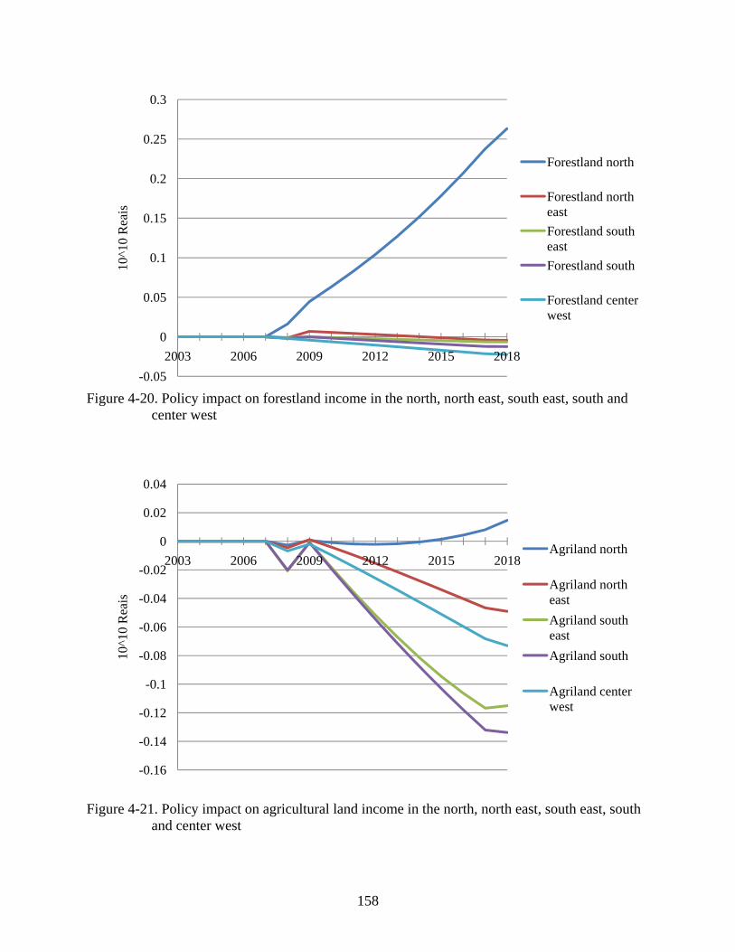
158
Figure 4-20. Policy impact on forestland income in the north, north east, south east, south and
center west
Figure 4-21. Policy impact on agricultural land income in the north, north east, south east, south and center west
-0.05
0
0.05
0.1
0.15
0.2
0.25
0.3
2003 2006 2009 2012 2015 2018
10^1
0 R
eais
Forestland north
Forestland north eastForestland south eastForestland south
Forestland center west
-0.16
-0.14
-0.12
-0.1
-0.08
-0.06
-0.04
-0.02
0
0.02
0.04
2003 2006 2009 2012 2015 2018
10^1
0 R
eais
Agriland north
Agriland north eastAgriland south eastAgriland south
Agriland center west

159
Figure 4-22. Policy impact on labor wages and the price of capital
Figure 4-23. Policy impact on price of forestland in the north, north east, south east, south and
center west
-0.008
-0.006
-0.004
-0.002
0
0.002
0.004
0.006
0.008
0.01
2003 2006 2009 2012 2015 201810^1
0 R
eais
Low-skilled labor wage
Mid-skilled labor wage
High-skilled labor wage
Capital price
-2.5
-2
-1.5
-1
-0.5
0
0.5
1
1.5
2
2.5
2003 2006 2009 2012 2015 2018
10^1
0 R
eais
Price of forestland north
Price of forestland north eastPrice of forestland south eastPrice of forestland south
Price of forestland center west

160
Figure 4-24. Policy impact on the price of agricultural land in the north, north east, south east,
south and center west
-0.4
-0.35
-0.3
-0.25
-0.2
-0.15
-0.1
-0.05
0
0.05
2003 2006 2009 2012 2015 2018
10^1
0 R
eais
Price of agriland northPrice of agriland north eastPrice of agriland south eastPrice of agriland southPrice of agriland center west

161
Table 4-1. Annual compound percent change in macroeconomic and institutional indicators between 2003 and 2018
Indicator Baseline Policy shock
Difference
Annual compound percent change Real household consumption (LCU at base prices) 5.9 5.9 0.0 Real investment (LCU at base prices) 6.2 6.2 0.0 Real government consumption (LCU at base prices) 4.4 4.4 0.0 Total real exports (LCU at base prices) 5.1 5.1 0.0 Total real imports (LCU at base prices) 5.8 5.8 0.0 Purchasing Power Parity real exchange rate (LCUs per FCU)
-0.3 -0.3 0.0
Consumer Price Index (100 for base) -0.2 -0.2 0.0 Investment (% of nominal GDP) 0.0 0.0 0.0 Private savings (% of nominal GDP) -0.6 -0.6 0.0 Foreign savings (% of nominal GDP) 0.0 0.0 0.0 Trade deficit (% of nominal GDP) 0.1 0.1 0.0 Government savings (% of nominal GDP) 0.6 0.6 0.0 Direct tax revenue (% of nominal GDP) 0.0 0.0 0.0 Real household consumption Low-income household 3.7 3.7 0.0 Mid-income household 5.6 5.6 0.0 High-income household 6.6 6.6 0.0 Deforestation enterprise 3.3 -9.2 -12.5 Equivalent Variation Low-income household 5.0 5.0 0.0 Mid-income household 8.6 8.7 0.1 High-income household 11.2 11.2 0.0 Deforestation enterprise 17.3 -3.0 -20.3 Nominal GDP at market prices 5.5 5.5 0.0 Nominal GDP at factor cost 5.6 5.6 0.0 Real GDP at market prices 5.5 5.5 0.0 Real GDP at factor cost 5.5 5.6 0.0 Notes: LCU and FCU are local and foreign currency units respectively

162
Table 4-2. Average annual growth rate in the level of domestic activity between 2003 to 2018 Activity Baseline
(%) Policy shock (%)
Difference (%)
Agriculture north 1.85 2.29 0.45 Agriculture north east 1.69 2.05 0.36 Agriculture south east 5.06 5.15 0.09 Agriculture south 2.00 2.17 0.18 Agriculture center west 1.65 1.60 -0.05 Legal forestry north -0.02 13.51 13.53 Legal forestry north east 5.91 3.69 -2.22 Legal forestry south east 1.18 1.10 -0.08 Legal forestry south 1.03 0.99 -0.04 Legal forestry center west -3.67 0.42 4.09 Illegal forestry north 1.65 12.24 10.59 Illegal forestry north east 5.37 2.58 -2.78 Illegal forestry center west -2.13 0.80 2.93 Forest plantations north 14.40 11.28 -3.11 Forest plantations north east 12.40 9.75 -2.65 Forest plantations south east -7.31 -9.19 -1.87 Forest plantations south 2.84 0.27 -2.56 Forest plantations center west 12.40 9.12 -3.28 Legal deforestation north 0.28 9.02 8.74 Legal deforestation north east -10.52 -0.60 9.92 Legal deforestation center west -0.55 9.67 10.22 Illegal deforestation north 5.07 -21.01 -26.08 Illegal deforestation north east -0.70 -8.17 -7.47 Illegal deforestation center west 3.19 -2.00 -5.19 Mining and petroleum 6.28 6.25 -0.02 Industry 5.72 5.73 0.01 Wood processing 4.05 4.43 0.38 Pulp and cellulose 3.49 4.24 0.75 Food processing 3.61 3.71 0.10 Utilities 5.92 5.94 0.02 Construction 6.04 6.07 0.03 Commerce 6.86 6.79 -0.08 Transportation 5.91 5.92 0.01 Private services 5.96 5.97 0.01 Public services 4.39 4.39 0.00

163
Table 4-3. Average annual growth rate in the quantity of composite supply between 2003 and 2018 Activity Baseline (%) Policy shock (%) Difference (%) Agriculture 3.90 3.98 0.09 Forestry 3.98 4.45 0.47 Deforestation 3.34 -9.19 -12.52 Mining and petroleum 5.72 5.74 0.01 Industrial 5.77 5.80 0.03 Processed wood 5.21 5.34 0.14 Pulp and cellulose 3.82 4.58 0.76 Processed food 4.72 4.78 0.05 Utilities 5.85 5.87 0.02 Construction 6.04 6.07 0.03 Commerce 6.42 6.37 -0.05 Transportation 5.90 5.91 0.01 Private services 5.94 5.95 0.01 Public services 4.39 4.39 0.00
Table 4-4. Average annual growth rate in the quantity of domestic and export sales between 2003 and 2018 Baseline Policy
shock Difference Baseline Policy
shock Difference
Good or service Domestic sales (%)
Domestic sales (%)
Domestic sales (%)
Exports (%)
Exports (%)
Exports (%)
Agriculture 3.56 3.66 0.10 0.91 1.12 0.21 Forestry 2.17 3.27 1.10 -4.28 -1.75 2.53 Deforestation 3.34 -9.19 -12.52 0.00 0.00 0.00 Mining and petroleum
5.95 5.95 0.00 7.03 6.96 -0.07
Industrial products
5.82 5.84 0.02 6.10 6.07 -0.03
Processed wood 5.16 5.31 0.15 2.36 3.22 0.86 Pulp and cellulose
3.78 4.54 0.76 3.39 4.13 0.74
Processed food 4.67 4.73 0.05 1.01 1.16 0.15 Utilities 5.91 5.92 0.02 0.00 0.00 0.00 Construction 6.04 6.07 0.03 6.25 6.27 0.02 Commerce 6.04 6.03 0.00 5.35 5.43 0.08 Transportation 5.90 5.91 0.01 6.10 6.08 -0.02 Private services 5.96 5.97 0.01 6.12 6.11 -0.01 Public services 4.39 4.39 0.00 0.00 0.00 0.00

164
Table 4-5. Average annual growth rate in composite commodity prices between 2003 and 2018
Good or service Baseline (%) Policy shock (%) Difference (%) Agriculture 1.68 1.59 -0.09 Forestry 4.23 3.29 -0.94 Deforestation 2.54 15.02 12.49 Mining and petroleum -0.78 -0.76 0.02 Industrial products -0.43 -0.43 0.01 Processed wood 0.89 0.57 -0.32 Pulp and cellulose -0.20 -0.20 0.00 Processed food 0.86 0.81 -0.04 Utilities -1.01 -0.99 0.02 Construction -0.75 -0.75 0.00 Commerce 0.52 0.41 -0.11 Transportation -0.59 -0.56 0.02 Private services -0.55 -0.54 0.02 Public services 1.29 1.31 0.02
Table 4-6. Average annual growth rate in the quantity of factor demand by industry between 2003 and 2018 Activity Factor Baseline
(%) Policy shock (%)
Difference (%)
Agriculture north Agricultural land north
0.91 1.39 0.48
Forest plantations north 13.41 10.35 -3.06 Agriculture north east Agricultural land
north east -0.05 0.45 0.50
Forest plantations north east 10.84 8.30 -2.54 Agriculture south east Agricultural land
south east 2.25 2.43 0.18
Forest plantations south east -8.45 -10.31 -1.87 Agriculture south Agricultural land
south -0.15 0.07 0.22
Forest plantations south 1.60 -0.95 -2.55 Agriculture center west Agricultural land
center west 0.56 0.51 -0.04
Forest plantations center west
11.34 8.07 -3.27
Legal forestry north Forestland north -1.13 12.56 13.69 Illegal forestry north 0.75 11.42 10.67 Legal deforestation north Forest land north -0.69 8.24 8.92

165
Table 4-6. Continued Activity Factor Baseline
(%) Policy shock (%)
Difference (%)
Illegal deforestation north 4.01 -21.78 -25.78 Legal forestry north east Forestland north east 3.55 1.40 -2.16 Illegal forestry north east 4.19 1.42 -2.77 Legal deforestation north east -11.56 -1.64 9.93 Illegal deforestation north east -1.92 -9.37 -7.45 Legal forestry south east Forestland south east 0.00 0.00 0.00 Legal forestry south Forestland south 0.00 0.00 0.00 Legal forestry center west Forestland center west -4.75 -0.61 4.14 Illegal forestry center west -3.02 -0.07 2.95 Legal deforestation center west -1.51 8.76 10.27 Illegal deforestation center west 2.15 -2.96 -5.10
Table 4-7. Average annual growth rate in institutional income between 2003 and 2018 Institution Baseline (%) Policy shock (%) Difference (%) Low income household 3.11 3.12 0.01 Mid-income household 4.79 4.81 0.02 High-income household 5.54 5.57 0.03 Deforestation institution 5.28 5.25 -0.04 Enterprises 5.88 5.90 0.02 Interest 5.28 5.31 0.03
Table 4-8. Average annual growth rate in factor income between 2003 and 2018 Factor Baseline (%) Policy shock (%) Difference (%) Low-skill labor 4.86 4.86 0.01 Mid-skill labor 5.03 5.05 0.03 High-skill labor 5.23 5.26 0.03 Capital 5.79 5.82 0.03 Agricultural land north 4.97 5.05 0.08 Agricultural land north east 8.04 7.55 -0.49 Agricultural land south east 11.09 10.61 -0.47 Agricultural land south 9.09 8.79 -0.30 Agricultural land center west 5.48 5.35 -0.14 Forest land north 9.22 14.61 5.39 Forest land north east 14.38 13.71 -0.66 Forest land south east 8.29 6.96 -1.32 Forest land south 7.64 6.50 -1.14 Forest land center west 9.69 7.30 -2.39

166
Table 4-9. Average annual growth rate in factor wages and prices between 2003 and 2018 Factor Baseline (%) Policy shock (%) Difference (%) Low-skill labor 3.69 3.70 0.01 Mid-skill labor 3.86 3.89 0.03 High-skill labor 4.07 4.10 0.03 Capital -1.46 -1.44 0.02 Agricultural land north 3.97 3.61 -0.36 Agricultural land north east 7.62 6.84 -0.78 Agricultural land south east 11.09 10.61 -0.47 Agricultural land south 9.09 8.79 -0.30 Agricultural land center west 4.87 4.80 -0.07 Forest land north 9.22 3.02 -6.20 Forest land north east 14.38 13.71 -0.66 Forest land south east 8.29 6.96 -1.32 Forest land south 7.64 6.50 -1.14 Forest land center west 9.69 7.30 -2.39

167
CHAPTER 5 CONCLUSIONS
Historical analysis suggests that forest policies of countries with significant forested
frontiers transition through stages of forest policy development reflecting the orientation of
governments toward economic development on the frontiers, namely: settlement, protective
custody and management. To present, with regards to the forests of the Amazon, Brazil is no
exception. The period of settlement as the name suggests was characterized by land clearing to
provide raw materials and establish farms and ranches. Policy makers could not, however, ignore
the apparent devastation that resulted, particularly in the Atlantic Forest Region, and passed the
first Forestry Code in 1934. A basic framework for forest concessions was included in the law,
although they were never implemented. With government priorities focusing on colonization and
agricultural expansion, the destruction continued largely unabated.
As forests in the Atlantic region continued to be reduced in quantity and quality and with
the poor implementation record of the 1934 Forestry Code, policy makers began to develop a
New Forestry Code which was subsequently approved in 1965. This New Code was significantly
more protectionist and marks the transition in forest policy development to the protective
custody phase. An important feature of this code is the limitation placed on private property
rights. During this period, protective legislation flourished, along with the creation of large
protected areas; initiatives to promote the development of the natural forest management sector
were lacking, however. With the forest plantation sector feeding the nation’s metal and mineral
industries, the provision and management of incentives for forest plantations was a substantial
component of forest policy. Institutions and programs during this period were weak and
underfunded, however, and although the forest policy framework developed significantly more
than in the previous period, the state’s prioritization of industrialization and integration of the

168
Amazon into the national economy resulted in the marginalization of forest policy rendering it
largely ineffectual. As such, the protectionist stage of Brazilian forest policy lived out primarily
on paper
Signs of change in the relevance of forestry and environmental policy began with the
political opening in 1974 when the seeds of an environmental movement were sown. The
movement, aligning itself with already established democratic and international environmental
movements, was successful in creating political space for the assertion of environmental
interests. Brazil’s democratization, the growing influence of environmental movements and civil
society’s effective engagement in political affairs pushed forest policy towards the management
stage of policy development by the beginning of the millennium. This transition is marked by
various forest and environment sector initiatives such as the National System of Nature
Conservation Units (SNUC), The National Forest Program (PNF), incentives for the
development of the natural forest management sector, and the Public Forest Management Law
(PFML). The PFML is of considerable interest; a significant component of the law involves the
authorization of forest concessions on public lands, whereas previous forest policies relating to
timber extraction were focused on the regulation of forestry on private land. Taking the PFML as
a proximate indicator of the transition to the management stage of forest policy development, the
variables that led to the political opening for the approval of the law are important to understand.
First, levels of deforestation reached historic heights in 1995 and 2002. With greater
transparency and domestic and international concern for the Amazon region, the state was
pushed to act in defense of the forest resources of the region and develop frameworks to combat
deforestation. Escalating violence caused by land tenure disputes, changes in the regulatory
framework for natural forest management, the ensuing scarcity of forestland for legal forestry,

169
and the resulting forest sector crisis urged the government to send the PFML proposal to
Congress as a constitutional emergency. Aided by the left-leaning Worker’s Party and greater
representation for the interests of forestry-based communities, the law passed swiftly through
Congress and was approved in March of 2006.
The level of success that is experienced in the implementation of the PFML will reveal
whether the new policies and institutions established since 2000 represent a break with the past
with regards to the low levels of policy implementation that characterized the protective custody
period. There are convincing reasons to believe that the management stage of forest policy will
be significantly more effectively implemented. Efforts to delimit public lands and state-civil
society partnerships are making progress in regulating public land use. With a globalized civil
society and media, the economic and political costs of the illegal exploitation of forest resources
are becoming a significant obstacle to illegality in the forest sector. The state has committed
unprecedented institutional support and funding towards gaining control of forest resources in
the Amazon. Various contradictory extra-sectoral policies have been eliminated. Furthermore,
the economic opportunities presented by sustainable forest management are increasing.
Payments for environmental services, carbon credits for carbon sequestration, and incentives for
avoided deforestation may serve to increase the value of standing, managed forests as opposed to
an agricultural alternative. The outlook for a transition to management that is lived out in
practice is decidedly optimistic.
Taking the PFML and the establishment of forest concessions in particular as a proximate
indicator of a substantive transition to the management phase of forest policy development, the
economic, welfare, and environmental response to concessions provides an indication of the
degree to which, if fully implemented, forest policy will be accepted and supported by society.
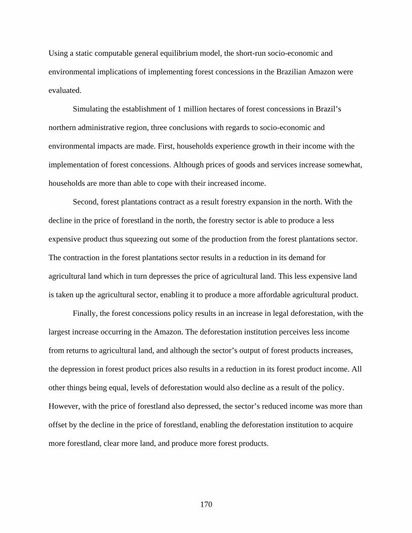
170
Using a static computable general equilibrium model, the short-run socio-economic and
environmental implications of implementing forest concessions in the Brazilian Amazon were
evaluated.
Simulating the establishment of 1 million hectares of forest concessions in Brazil’s
northern administrative region, three conclusions with regards to socio-economic and
environmental impacts are made. First, households experience growth in their income with the
implementation of forest concessions. Although prices of goods and services increase somewhat,
households are more than able to cope with their increased income.
Second, forest plantations contract as a result forestry expansion in the north. With the
decline in the price of forestland in the north, the forestry sector is able to produce a less
expensive product thus squeezing out some of the production from the forest plantations sector.
The contraction in the forest plantations sector results in a reduction in its demand for
agricultural land which in turn depresses the price of agricultural land. This less expensive land
is taken up the agricultural sector, enabling it to produce a more affordable agricultural product.
Finally, the forest concessions policy results in an increase in legal deforestation, with the
largest increase occurring in the Amazon. The deforestation institution perceives less income
from returns to agricultural land, and although the sector’s output of forest products increases,
the depression in forest product prices also results in a reduction in its forest product income. All
other things being equal, levels of deforestation would also decline as a result of the policy.
However, with the price of forestland also depressed, the sector’s reduced income was more than
offset by the decline in the price of forestland, enabling the deforestation institution to acquire
more forestland, clear more land, and produce more forest products.

171
Given the significant economic importance of the illegal forestry and illegal deforestation
sectors in Brazil and to more realistically evaluate the socio-economic and environmental
impacts of forest concessions, illegal forestry and illegal deforestation sectors are disaggregated
and modeled. A recursive dynamic computable general equilibrium modeling framework is
chosen to consider the medium-term implications of the implementation of forest concessions.
Advantages of the dynamic modeling framework include: the ability to update the factor supply
of agricultural land based on annual levels of deforestation; the model sheds light on the
economic transition path resulting from the policy shock; and, it provides information on the
short-term costs and longer-term gains resulting from policy implementation. The baseline
scenario projects the Brazilian economy from 2003 to 2018 by accounting for growth in the labor
force, population, and total factor productivity, as well as accounting for capital accumulation
and depreciation. The policy shock scenario uses the results of the baseline scenario and
introduces the forest concessions shock into the economy. The difference between the value of
indicators in the baseline and the policy shock scenario is the net policy impact of forest
concessions.
The overall policy impact of forest concessions on the Brazilian economy is relatively
small with the exception of the negative welfare impact on the illegal deforestation institution. In
the absence of forest concessions, legal forestry activities contract in the north and center west.
Increased demand for forest products is met by relatively large growth in forest plantations with
the exception of the south east. Introducing the concessions policy, legal forestry in the north and
center west expand, which may be an indication of the current scarcity of forestland for legal
forestry operations. Illegal forestry activities increase in the baseline in the north and north east
and decrease in the center west; in the policy scenario, growth in activity increases dramatically

172
in the north and to a slightly lesser degree in the center west, while growth is reduced in the north
east.
Legal deforestation in the baseline expands slightly in the north and contracts in the north
east and center west. The policy impact, however, leads to faster growth in all regions. It should
be noted that although growth rates in legal deforestation activities are large, the legal
deforestation sector’s output of forest products and demand for forestland is initially quite small.
Illegal deforestation grows in the north and center west and contracts in the north east in the
baseline; the policy impact, however, results in a contraction in all regions. This contraction in
illegal deforestation is a function of the increasing scarcity of forestland on which firms may
operate illegally and the reduced returns to agricultural land which fund the deforestation
institution. In addition, since legal deforestation is able to more fully utilize timber prior to land
clearing, it is able to out-compete the illegal deforestation sectors in terms of forest product
output. The overall policy impact of forest concessions on illegality is to reduce the rate of
growth of illegal forestry in the north east and reduce the level of illegal deforestation in all
regions; the legal deforestation sectors grow faster as a result of the policy.
As a result of increased forest product output from legal and illegal forestry and legal
deforestation in the north, the forest plantations sectors experience a negative policy impact in all
regions. Nonetheless, forest plantation activities continue to grow with the exception of the south
east. With increased supply of raw materials from forest product producing sectors, the
processed wood, and pulp and cellulose sectors grow at a faster rate as a result of the policy.
Both domestic and export demand increase for forestry, agricultural, processed wood, and pulp
and cellulose products. Agricultural and forest product prices grow at a slower rate as a result of
forest concessions.

173
Agricultural activity grows in all regions in the baseline; the policy impact is positive in
all regions with the exception of a small reduction in growth in the center west. While the greater
rate of expansion in the north and north east are a function of faster rates of legal deforestation
(i.e. the production of agricultural land) as well as the forest plantations sectors’ reduced demand
for agricultural land, the decline in the center west appears to be the result of a relatively large
decrease in illegal deforestation, given the importance of this sector in generating agricultural
land.
With regards to household income, the policy impact is positive. Since high and mid-
income households receive a greater share of income from legal and illegal deforestation among
other things, their incomes grow at a faster rate. Low-income and mid-income households
experience an adjustment period to the policy shock with their incomes negatively affected for a
short period in comparison to the baseline. The overall impact on income growth over the time
period, however, is positive.
In the baseline, labor and capital income increase; forest concessions have a positive
impact on the income of all labor classes as well as capital due to increased growth in demand
and higher rates of growth in wages. The policy impact on growth of forestland income is
positive and large in the north and negative in other regions. With the price of forestland
negatively impacted by the policy in all regions, the increase in income in the north is explained
by the increase in the stock and demand for forestland. With regards to agricultural land income,
the average growth rate in all regions is increasing in the baseline. The policy impact is large and
positive in the north and negative in all other regions. With all regions experiencing growth in
demand for agricultural land in the policy scenario with the exception of the center west, the
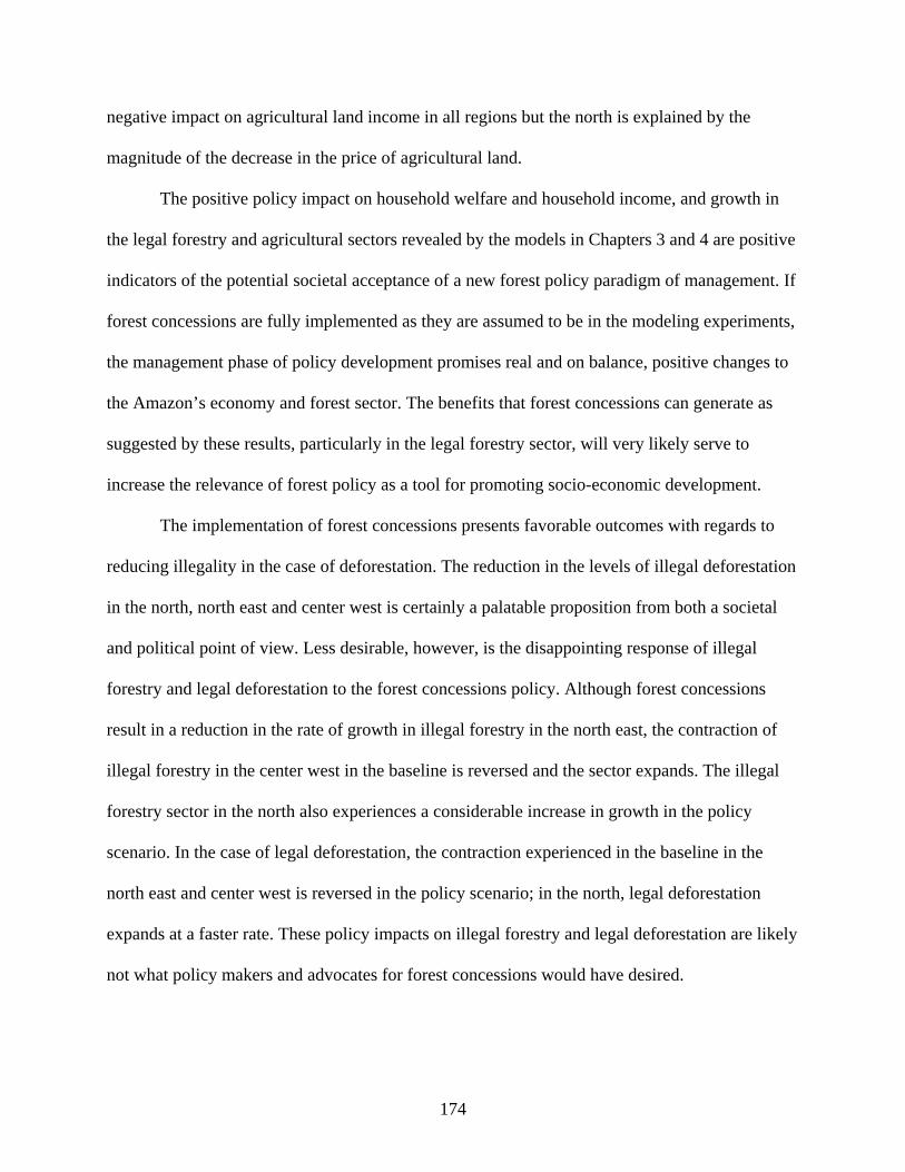
174
negative impact on agricultural land income in all regions but the north is explained by the
magnitude of the decrease in the price of agricultural land.
The positive policy impact on household welfare and household income, and growth in
the legal forestry and agricultural sectors revealed by the models in Chapters 3 and 4 are positive
indicators of the potential societal acceptance of a new forest policy paradigm of management. If
forest concessions are fully implemented as they are assumed to be in the modeling experiments,
the management phase of policy development promises real and on balance, positive changes to
the Amazon’s economy and forest sector. The benefits that forest concessions can generate as
suggested by these results, particularly in the legal forestry sector, will very likely serve to
increase the relevance of forest policy as a tool for promoting socio-economic development.
The implementation of forest concessions presents favorable outcomes with regards to
reducing illegality in the case of deforestation. The reduction in the levels of illegal deforestation
in the north, north east and center west is certainly a palatable proposition from both a societal
and political point of view. Less desirable, however, is the disappointing response of illegal
forestry and legal deforestation to the forest concessions policy. Although forest concessions
result in a reduction in the rate of growth in illegal forestry in the north east, the contraction of
illegal forestry in the center west in the baseline is reversed and the sector expands. The illegal
forestry sector in the north also experiences a considerable increase in growth in the policy
scenario. In the case of legal deforestation, the contraction experienced in the baseline in the
north east and center west is reversed in the policy scenario; in the north, legal deforestation
expands at a faster rate. These policy impacts on illegal forestry and legal deforestation are likely
not what policy makers and advocates for forest concessions would have desired.
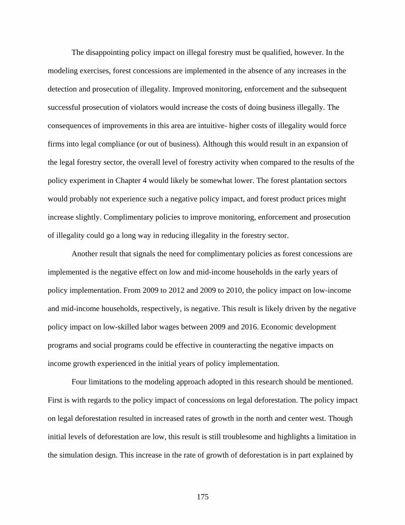
175
The disappointing policy impact on illegal forestry must be qualified, however. In the
modeling exercises, forest concessions are implemented in the absence of any increases in the
detection and prosecution of illegality. Improved monitoring, enforcement and the subsequent
successful prosecution of violators would increase the costs of doing business illegally. The
consequences of improvements in this area are intuitive- higher costs of illegality would force
firms into legal compliance (or out of business). Although this would result in an expansion of
the legal forestry sector, the overall level of forestry activity when compared to the results of the
policy experiment in Chapter 4 would likely be somewhat lower. The forest plantation sectors
would probably not experience such a negative policy impact, and forest product prices might
increase slightly. Complimentary policies to improve monitoring, enforcement and prosecution
of illegality could go a long way in reducing illegality in the forestry sector.
Another result that signals the need for complimentary policies as forest concessions are
implemented is the negative effect on low and mid-income households in the early years of
policy implementation. From 2009 to 2012 and 2009 to 2010, the policy impact on low-income
and mid-income households, respectively, is negative. This result is likely driven by the negative
policy impact on low-skilled labor wages between 2009 and 2016. Economic development
programs and social programs could be effective in counteracting the negative impacts on
income growth experienced in the initial years of policy implementation.
Four limitations to the modeling approach adopted in this research should be mentioned.
First is with regards to the policy impact of concessions on legal deforestation. The policy impact
on legal deforestation resulted in increased rates of growth in the north and center west. Though
initial levels of deforestation are low, this result is still troublesome and highlights a limitation in
the simulation design. This increase in the rate of growth of deforestation is in part explained by

176
the fact that the legal deforestation sector is not constrained by increasing factor scarcity of
private forestland, rather, it is constrained by the total supply of forestland. For deforestation to
be legal, it must be legally authorized on private land. Private property owners in the Amazon are
permitted by law to clear up to 20% of their forestland. The amount of forest area that can legally
be cleared on private land, however, is likely somewhat scarce; reliable estimates of the size of
this area are required to increase the realism of the simulation with regards to forestland
constraints on the legal deforestation sector.
The second limitation is elucidated by the policy impact on the illegal forestry sector. The
illegal forestry sector’s use of forestland is constrained by the total supply of forestland. The
potential increasing scarcity of forestland for illegal activities is modeled as reduced yields per
unit of illegal forestry activity. With the implementation of forest concessions, the 1 million
hectare per year increase in forestland stock is made available to all forest product producing
sectors. With the implementation of forest concessions, however, both the state and the
concessionaire have a vested interest in prohibiting the illegal logging or clearing of the
concession by a third party. Illegal activities engaged in by the concessionaire aside (i.e. over-
harvesting, under-reporting, harvesting in sensitive areas), it is expected that the level of
monitoring and enforcement in the concession and in proximity to the concession would increase
as a result of the policy. To some degree, this heightened vigilance is modeled by the illegal
forestry sector’s reduced yields per unit of activity. The real effect of concessions in reducing the
availability of forestland for illegal operations is uncertain, however, though it is likely lower
than that modeled in Chapter 4.
The third model limitation is with regards to the world prices of goods and services.
World prices and therefore export prices remain constant in the dynamic modeling experiment.

177
Often, depending on the time horizon of analysis, world prices are updated according to
projections made by industry experts. The highly aggregated social accounting matrix developed
for this analysis, however, is not conducive to exogenously updating world prices. For example,
the industrial sector produces everything from leather goods to motor vehicles, whose general
rate of growth in prices may be quite different. To avoid erroneous conclusions that may be
driven by the inflexibility in the world price system as modeled, a medium-term time horizon of
10 years was chosen. Since domestic prices are allowed some flexibility in the model due to
imperfect substitution between imported goods and domestically produced goods, domestic
prices tend to grow while export prices remain constant. The implications of fixed world prices
on the modeling results are a likely lower growth rate in exports than would occur if world prices
were updated according to industry projections.
Finally, the fourth limitation to the modeling approach involves the aggregation of
households. Disaggregation of households according to region would be advantageous to
understand the regional income impacts of policy implementation. As the results from Chapters 3
and 4 indicate, there is a small increase in aggregate household income and welfare. With a
regional disaggregation of households, the policy impact on household income growth in the
northern region would likely prove to be substantially greater than in other regions. Data
limitations, however, restricted the current analysis of household income to the economy-wide
aggregate level.
Three areas for promising future research may be mentioned. First, the policy experiment
is conducted in the absence of potential increases in the detection and prosecution of illegal
deforestation and illegal forestry. The computable general equilibrium framework applied in this
research is conducive to iteratively and exogenously shocking the value of the fine paid per unit

178
of illegal output. Determining the level of fines that would be required to reduce illegal forestry
and illegal deforestation to the socially optimal level would be useful to policy makers in their
decisions on budgetary allocations for monitoring and enforcement.
Second, policy makers may be interested in the longer run (10+ years) socioeconomic
and environmental impacts of forest concessions. The debate surrounding Reduced Emissions
from Deforestation and Degradation can significantly increase the demand for this type of
information. A greater disaggregation of the social accounting matrix for Brazil in terms of
activities, commodities and households, as well as estimates on changes in the world price of
goods and services would enable more realistic, longer-term analysis of the impacts of forest
concessions.
Finally, the modeling exercises treat forestland as capable of producing the same quantity
and quality of forest product output through time. Forestry law sets diameter, species and volume
constraints on forest operations. Whether these limits, assuming they are followed, result in
sustainable yields is an open question, though recent research appears to indicate that they are
not. In the short and medium term as modeled in the current analysis, declining quantity and
quality of timber stocks may not present any measurable impact. If the policy is modeled in the
longer-term, however, interesting results may be borne out of modeling changes in the
characteristics of the timber supply.
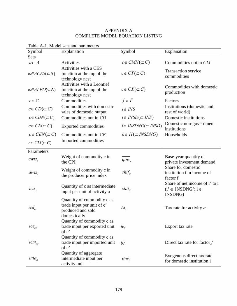
179
APPENDIX A COMPLETE MODEL EQUATION LISTING
Table A-1. Model sets and parameters Symbol Explanation Symbol Explanation Sets
Activities Commodities not in CM
ACES( A) Activities with a CES function at the top of the technology nest
Transaction service commodities
ALEO( A) Activities with a Leontief function at the top of the technology nest
Commodities with domestic production
Commodities Factors
Commodities with domestic sales of domestic output Institutions (domestic and
rest of world) Commodities not in CD Domestic institutions
Exported commodities Domestic non-government institutions
Commodities not in CE Households
( )c CM C∈ ⊂ Imported commodities
Parameters Weight of commodity c in
the CPI Base-year quantity of private investment demand
Weight of commodity c in the producer price index
Share for domestic institution i in income of factor f
Quantity of c as intermediate input per unit of activity a
Share of net income of i’ to i (i’ ∈ INSDNG’; i ∈ INSDNG)
Quantity of commodity c as trade input per unit of c’ produced and sold domestically
Tax rate for activity a
Quantity of commodity c as trade input per exported unit of c’
tec Export tax rate
Quantity of commodity c as trade input per imported unit of c’
tff Direct tax rate for factor f
Quantity of aggregate intermediate input per activity unit
Exogenous direct tax rate for domestic institution i
a A∈ ( )c CMN C∈ ⊂
( )c CT C∈ ⊂
( )c CX C∈ ⊂
c C∈ f F∈
( )c CD C∈ ⊂ i INS∈
( )c CDN C∈ ⊂ ( )i INSD INS∈ ⊂
( )c CE C∈ ⊂ ( )i INSDNG INSD∈ ⊂
( )c CEN C∈ ⊂ ( )h H INSDNG∈ ⊂
ccwts cqinv
cdwts ifshif
caica 'iishii
'ccicd ata
'ccice
'ccicm
ainta itins

180
Table A-1. Continued Symbol Explanation Symbol Explanation
Quantity of aggregate intermediate input per activity unit
0-1 parameter with 1 for institutions with potentially flexed direct tax rates
Base savings rate for domestic institution i
Import tariff rate
0-1 parameter with 1 for institutions with potentially flexed direct tax rates
Rate of sales tax
Export price (foreign currency)
Transfer from factor f to institution i
Import price (foreign currency) tvaa
Rate of value-added tax for activity a
Quantity of stock change
Base-year quantity of government demand
Greek letters
Efficiency parameter in the CES activity function CET function share
parameter
Efficiency parameter in the CES value-added function
CES value-added function share parameter for factor f in activity a
Shift parameter for domestic commodity aggregation function
Subsistence consumption of marketed commodity c for household h
Armington function shift parameter
Yield of output c per unit of activity a
CET function shift parameter CES production function exponent
aβ Capital sectoral mobility factor CES value-added function
exponent
βhach
Marginal share of consumption spending on home commodity c from activity a for household h
Domestic commodity aggregation function exponent
Marginal share of consumption spending on marketed commodity c for household h
Armington function exponent
CES activity function share parameter CET function exponent
Share parameter for domestic commodity aggregation function
afatη Sector share of new capital
(dynamic model)
aiva itins01
imps ctm
imps01 ctq
cpwe i ftrnsfr
cpwm
cqdst
cqg
aaα
tcδ
vaaα
vafaδ
accα
mchγ
qcα acθ
tcα
aaρ
vaaρ
accρ
mchβ q
cρ
aaδ
tcρ
acacδ
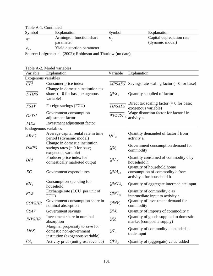
181
Table A-1. Continued Symbol Explanation Symbol Explanation
Armington function share parameter
fυ Capital depreciation rate (dynamic model)
ca ,ϕ Yield distortion parameter Source: Lofgren et al. (2002); Robinson and Thurlow (no date). Table A-2. Model variables Variable Explanation Variable Explanation Exogenous variables
Consumer price index Savings rate scaling factor (= 0 for base)
Change in domestic institution tax share (= 0 for base; exogenous variable)
Quantity supplied of factor
Foreign savings (FCU) Direct tax scaling factor (= 0 for base; exogenous variable)
Government consumption adjustment factor
Wage distortion factor for factor f in activity a
Investment adjustment factor Endogenous variables
aftAWF
Average capital rental rate in time period t (dynamic model)
Quantity demanded of factor f from activity a
Change in domestic institution savings rates (= 0 for base; exogenous variable)
Government consumption demand for commodity
Producer price index for domestically marketed output
Quantity consumed of commodity c by household h
Government expenditures Quantity of household home consumption of commodity c from activity a for household h
Consumption spending for household
Quantity of aggregate intermediate input
Exchange rate (LCU per unit of FCU)
Quantity of commodity c as intermediate input to activity a
Government consumption share in nominal absorption
Quantity of investment demand for commodity
Government savings Quantity of imports of commodity c
Investment share in nominal absorption
Quantity of goods supplied to domestic market (composite supply)
Marginal propensity to save for domestic non-government institution (exogenous variable)
Quantity of commodity demanded as trade input
Activity price (unit gross revenue) Quantity of (aggregate) value-added
qcδ
CPI MPSADJ
DTINS fQFS
FSAV TINSADJ
GADJ faWFDIST
IADJ
faQF
DMPS cQG
DPI chQH
EG achQHA
hEH aQINTA
EXR caQINT
GOVSHR cQINV
GSAV cQM
INVSHR cQQ
iMPS cQT
aPA aQVA

182
Table A-2. Continued Variable Explanation Variable Explanation
Demand price for commodity produced and sold domestically
Aggregated quantity of domestic output of commodity
Supply price for commodity produced and sold domestically
Quantity of output of commodity c from activity a
Export price (domestic currency) fRWF Real average factor price (dynamic model)
Aggregate intermediate input price for activity a Total nominal absorption
ftPK Unit price of capital in time period t (dynamic model)
Direct tax rate for institution i (i ∈ INSDNG)
Import price (domestic currency) Transfers from institution i’ to i (both in the set INSDNG)
Composite commodity price Average price of factor
Value-added price (factor income per unit of activity)
Income of factor f
Aggregate producer price for commodity Government revenue
Producer price of commodity c for activity a
Income of domestic non-government institution
Quantity (level) of activity Income to domestic institution i from factor f
Quantity sold domestically of domestic output
afatKΔ Quantity of new capital by activity a for
time period t (dynamic model) Quantity of exports
Source: Lofgren et al. (2002); Robinson and Thurlow (no date). Table A-3. Model equations
ccCTc
cccc icmPQEXRtmpwmPM ''
')1( ⋅+⋅+⋅= ∑∈
(1)
ccCTc
cccc icePQEXRtepwePE ''
')1( ⋅−⋅−⋅= ∑∈
(2)
ccCTc
ccc icdPQPDSPDD ''
' ⋅+= ∑∈
(3)
ccccccc QMPMQDPDDQQtqPQ ⋅+⋅=⋅−⋅ )1( (4)
cccccc QEPEQDPDSQXPX ⋅+⋅=⋅ (5)
acCc
aca PXACPA θ⋅= ∑∈
(6)
caCc
ca icaPQPINTA ⋅= ∑∈
(7)
aaaaaa QINTAPINTAQVAPVAQAtaPA ⋅+⋅=⋅−⋅ )1( (8)
cCc
c cwtsPQCPI ⋅= ∑∈
(9)
cPDD cQX
cPDS acQXAC
cPE
aPINTA TABS
iTINS
cPM 'iiTRII
cPQ fWF
aPVA fYF
cPX YG
acPXAC iYI
aQA ifYIF
cQD
cQE
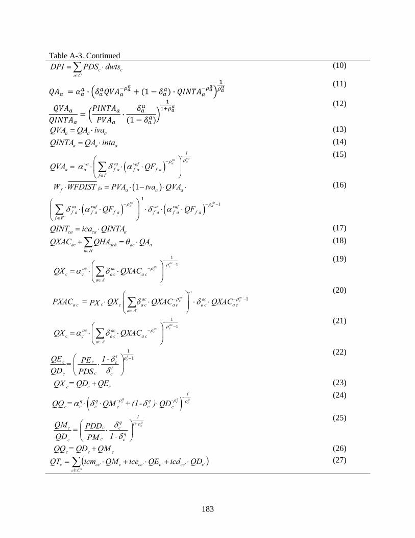
183
Table A-3. Continued
cCc
c dwtsPDSDPI ⋅= ∑∈
(10)
· 1 · (11)
· 1 (12)
aaa ivaQAQVA ⋅= (13)
aaa intaQAQINTA ⋅= (14)
( )vava aa
1-
va va vafa a f a f a f a
f FQVA QF
ρρα δ α
−
∈
⎛ ⎞= ⋅ ⋅ ⋅⎜ ⎟
⎝ ⎠∑
(15)
( )
( ) ( )1
1
'
1
va vaa a
faf a a a
va vaf va vaff a f a f a f a f a f a
f F
W WFDIST PVA tva QVA
QF QFρ ρ
δ α δ α−
− − −
∈
⋅ = ⋅ − ⋅ ⋅
⎛ ⎞⋅ ⋅ ⋅ ⋅ ⋅⎜ ⎟
⎝ ⎠∑
(16)
acaca QINTAicaQINT ⋅= (17)
aacHh
achac QAQHAQXAC ⋅=+∑∈
θ (18)
11ac
caccac ac
c c a c a ca A
QX QXACρ
ρα δ−
−−
∈
⎛ ⎞= ⋅ ⋅⎜ ⎟
⎝ ⎠∑
(19)
1
1
'
ac acc cac ac
ca c c a c a c a c a ca A
PXAC = QX QXAC QXACPX ρ ρδ δ−
− − −
∈
⎛ ⎞⋅ ⋅ ⋅ ⋅⎜ ⎟⎜ ⎟
⎝ ⎠∑
(20)
11ac
caccac ac
c c a c a ca A
QX QXACρ
ρα δ−
−−
∈
⎛ ⎞= ⋅ ⋅⎜ ⎟
⎝ ⎠∑
(21)
11t
ct
cc ct
c cc
QE 1 - PE = QD PDS
ρδδ
−⎛ ⎞⋅⎜ ⎟
⎝ ⎠
(22)
c cc = QD QEQX + (23)
( )q q qc c c
1-- -q q q
c c cc c c = + (1- )QQ QM QDρ ρ ρα δ δ⋅ ⋅ ⋅ (24)
qc
1q 1+
cc cq
c cc
QM PDD =1 - QD PM
ρδδ
⎛ ⎞⋅⎜ ⎟
⎝ ⎠
(25)
c c c = QQ QD QM+ (26) ( )∑
∈
⋅+⋅+⋅=''
'''''Cc
cccccccccc QDicdQEiceQMicmQT (27)

184
Table A-3. Continued Institutions
fafaAa
ff QFWFDISTWFYF ⋅⋅= ∑∈
(28)
i f i f f row fYIF = shif YF trnsfr EXR⎡ ⎤⋅ − ⋅⎣ ⎦ (29)
'' '
i i f i i i gov i rowf F i INSDNG
YI = YIF TRII trnsfr CPI trnsfr EXR∈ ∈
+ + ⋅ + ⋅∑ ∑ (30)
'' ' ' 'ii i i i i iTRII = shii (1- MPS ) (1- tins ) YI⋅ ⋅ ⋅ (31)
( )1 1 hh i h h hi INSDNG
EH = shii MPS (1- tins ) YI∈
⎛ ⎞− ⋅ − ⋅ ⋅⎜ ⎟
⎝ ⎠∑
(32)
' ' ' '' '
m m m mc ch c ch ch h c c h ac ac h
c C a A c CPQ QH PQ EH PQ PXACγ β γ γ
∈ ∈ ∈
⎛ ⎞⋅ = ⋅ + ⋅ − ⋅ − ⋅⎜ ⎟
⎝ ⎠∑ ∑∑
(33)
' ' ' '' '
h h m mac ach ac ach ach h c c h ac ac h
c C a A c CPXAC QHA PXAC EH PQ PXACγ β γ γ
∈ ∈ ∈
⎛ ⎞⋅ = ⋅ + ⋅ − ⋅ − ⋅⎜ ⎟
⎝ ⎠∑ ∑∑
(34)
c cQINV = IADJ qinv⋅ (35)
c cQG = GADJ qg⋅ (36)
i ai a ca c ci INSDNG a A c CMNR
cr c c c gov f gov rowcr crr R c CMR c C f F
YG tins YI ta tm EXRQA pwm QMPA
tmr EXR tq PQ QQ YF trnsfr EXRpwmr QMR∈ ∈ ∈
∈ ∈ ∈ ∈
= ⋅ + ⋅ ⋅ + ⋅ ⋅ +⋅
⋅ ⋅ + ⋅ ⋅ + + ⋅⋅
∑ ∑ ∑
∑ ∑ ∑ ∑
(37)
c c i govc C i INSDNG
EG PQ QG trnsfr CPI∈ ∈
= ⋅ + ⋅∑ ∑ (38)
System constraints f a f
a AQF QFS
∈
=∑ (39)
c c a c h c c c ca A h H
QQ QINT QH QG QINV qdst QT∈ ∈
= + + + + +∑ ∑ (40)
c c cr cr row fc CMNR r R c CMR f F
c c cr cr i rowc CENR r R c CER i INSD
pwm QM pwmr QMR trnsfr
pwe QE pwer QER trnsfr FSAV∈ ∈ ∈ ∈
∈ ∈ ∈ ∈
⋅ + ⋅ ⋅
= ⋅ + ⋅ + +
∑ ∑ ∑ ∑
∑ ∑ ∑ ∑
(41)
YG EG GSAV= + (42) · 1 · 01 · 01 (43) (1 01 ) 01i i iiMPS mps MPSADJ mps DMPS mps= ⋅ + ⋅ + ⋅ (44)
( )1 ii i c c c ci INSDNG c C c C
MPS tins YI GSAV EXR FSAV PQ QINV PQ qdst∈ ∈ ∈
⋅ − ⋅ + + ⋅ = ⋅ + ⋅∑ ∑ ∑ (45)
c ch ac achh H c C a A c C h H
c c c c c cc C c C c C
TABS PQ QH PXAC QHA
PQ QG PQ QINV PQ qdst∈ ∈ ∈ ∈ ∈
∈ ∈ ∈
= ⋅ + ⋅
+ ⋅ + ⋅ + ⋅
∑∑ ∑∑∑
∑ ∑ ∑
(46)

185
Table A-3. Continued c c c c
c C c CINVSHR TABS PQ QINV PQ qdst
∈ ∈
⋅ = ⋅ + ⋅∑ ∑ (47)
c cc C
GOVSHR TABS PQ QG∈
⋅ = ⋅∑ (48)
Capital accumulation (dynamic model)
'
f a taf t f t f a t
a f a' ta
QFAWF WF WFDIST
QF
⎡ ⎤⎛ ⎞⎢ ⎥⎜ ⎟= ⋅ ⋅⎢ ⎥⎜ ⎟⎜ ⎟⎢ ⎥⎝ ⎠⎣ ⎦
∑ ∑
(49)
,
'
1 1f a t f t f a ta af a t a
f a' t f ta
QF WF WFDISTQF AWF
η β⎛ ⎞ ⎛ ⎞⎛ ⎞⋅⎜ ⎟= ⋅ ⋅ − +⎜ ⎟⎜ ⎟⎜ ⎟ ⎜ ⎟⎜ ⎟⎜ ⎟ ⎝ ⎠⎝ ⎠⎝ ⎠∑
(50)
c t c ta a cf a t f a t
f t
PQ QINVK
PKη
⎛ ⎞⋅⎜ ⎟Δ = ⋅⎜ ⎟⎜ ⎟⎝ ⎠
∑
(51)
'
c tf t c t
c c' tc
QINVPK PQQINV
= ⋅∑ ∑
(52)
1af a t
f a t+1 f a t ff a t
KQF QF
QFυ
⎛ ⎞Δ= ⋅ + −⎜ ⎟⎜ ⎟
⎝ ⎠
(53)
1 1f a t
af t f t f
f t
KQFS QFS
QFSυ+
⎛ ⎞Δ⎜ ⎟= ⋅ + −⎜ ⎟⎜ ⎟⎝ ⎠
∑
(54)
Source: Lofgren et al. (2002); Robinson and Thurlow (no date).

186
APPENDIX B STATIC MODEL RESULTS: COMPARING THE BALANCED, NEOCLASSICAL AND
JOHANSEN CLOSURES
Table B-1. Percent change in macroeconomic and institutional indicators Balanced closure Neo classical closure Johansen closureAbsorption 0.01 0.00 0.01 Private consumption 0.02 -0.09 0.02 Fixed investment 0.00 0.39 0.00 Change in stocks 0.00 0.00 0.00 Government consumption 0.00 0.00 0.00 Exports 0.00 -0.11 -0.04 Imports -0.01 -0.13 -0.04 GDP at market prices 0.01 0.00 0.01 GDP at factor cost 0.01 0.01 0.01 Net indirect taxes 0.01 0.00 0.01 Real household consumption Low-income household 0.00 2.10 0.70 Mid-income household 0.00 0.20 0.10 High-income household 0.00 -0.90 -0.20 Deforestation enterprise 0.80 0.80 0.80 Consumer price index 0.02 -1.19 2.00 Exchange rate -0.01 -0.91 2.00 Investment share of absorption 0.00 30.77 3.32 Foreign savings 0.00 0.00 0.00 Marginal propensity to save Mid-income households 0.57 0.01 -218.82 High-income households 0.04 0.15 -14.11 Enterprises 0.01 0.41 -5.35 Investment to GDP ratio 0.00 4.70 0.50 Private savings to GDP ratio 0.00 0.60 -2.10 Foreign savings to GDP ratio 0.00 0.00 0.00 Trade deficit to GDP ratio 0.00 0.00 -0.10 Government savings to GDP ratio 0.00 4.10 2.60

187
Table B-2. Percent change in institutional income Institution Balanced closure Neo classical closure Johansen closure Low income household 0.05 0.96 0.49 Mid-income household 0.05 -0.99 -0.07 High-income household 0.04 -2.13 -0.80 Deforestation institution -0.24 -0.82 1.87 Enterprises 0.01 4.88 0.92 Interest 0.02 2.81 3.78 Table B-3. Percent change in equivalent variation Balanced closure Neoclassical closure Johansen closure
Equivalent variation Low-income households
0.00 2.10 0.70
Mid-income households
0.00 0.20 0.10
High-income households
0.00 -0.90 -0.20
Deforestation enterprise
0.80 0.80 0.80
Total 0.00 -0.10 0.00

188
Table B-4. Percent change in factor income Factor Balanced closure Neo classical closure Johansen closure Low-skill formal labor 0.08 -2.24 -2.81 Low-skill informal labor 0.07 14.64 1.30 Mid-skill formal labor 0.08 -10.53 -6.50 Mid-skill informal labor 0.07 -1.51 -1.96 High-skill formal labor 0.07 -16.38 -10.58 High-skill informal labor 0.08 -9.29 -4.89 Capital 0.13 5.30 0.98 Agricultural land north -0.17 -0.77 1.94 Agricultural land north east -0.38 -0.94 1.73 Agricultural land south east -6.79 -7.26 -4.81 Agricultural land south -1.81 -2.37 0.27 Agricultural land center west -0.17 -0.75 1.94 Forest land north -48.13 -48.37 -47.03 Forest land north east -14.25 -14.55 -12.37 Forest land south east -9.40 -9.93 -7.51 Forest land south -9.54 -10.06 -7.65 Forest land center west -11.14 -11.59 -9.27 Table B-5. Percent change in price of composite good Good or service Balanced closure Neo classical closure Johansen closure Agriculture -0.21 -0.88 1.88 Forestry -8.44 -9.03 -6.54 Deforestation -1.07 -1.64 3.22 Mining and petroleum -0.01 -0.91 2.00 Industrial 0.01 -0.92 2.01 Processed wood -0.01 -0.91 2.00 Pulp and cellulose -0.01 -0.91 2.00 Processed food 0.02 -0.74 2.12 Utilities 0.05 -0.95 2.12 Construction 0.17 69.40 2.00 Commerce -0.01 -0.91 2.00 Transportation 0.09 -1.36 2.07 Private services 0.05 -1.53 1.95 Public services 0.04 -20.85 -15.04

189
Table B-6. Percent change in price of factor F for activity A
Factor Sector Balanced closure
Neo classical closure Johansen closure
Low-skilled formal labor Agriculture north -0.13 -0.74 1.97 Low-skilled formal labor
Agriculture north east -0.11 -0.68 2.01
Low-skilled formal labor
Agriculture south east 0.54 0.06 2.70
Low-skilled formal labor Agriculture south 0.32 -0.27 2.44 Low-skilled formal labor
Agriculture center west -0.13 -0.71 1.98
Low-skilled formal labor Forestry north 143.65 142.52 148.80 Low-skilled formal labor Forestry north east -14.82 -15.10 -13.00 Low-skilled formal labor Forestry south east -9.40 -9.93 -7.51 Low-skilled formal labor Forestry south -9.54 -10.06 -7.65 Low-skilled formal labor Forestry center west -11.18 -11.63 -9.32 Low-skilled formal labor
Forest plantations north -13.57 -13.98 -11.75
Low-skilled formal labor
Forest plantations north east -14.40 -14.78 -12.59
Low-skilled formal labor
Forest plantations south east -20.43 -20.87 -18.78
Low-skilled formal labor
Forest plantations south -26.08 -26.29 -24.52
Low-skilled formal labor
Forest plantations center west -15.99 -16.40 -14.23
Low-skilled formal labor Deforestation north 18.84 18.15 22.68 Low-skilled formal labor
Deforestation north east -6.96 -7.50 -4.34
Low-skilled formal labor
Deforestation center west -5.89 -6.42 -2.92
Low-skilled formal labor
Mining and petroleum -0.09 -3.44 1.99
Low-skilled formal labor Industry 0.01 -1.22 2.02 Low-skilled formal labor Processed wood 2.68 1.85 4.73

190
Table B-6. Continued
Factor Sector Balanced closure Neoclassical closure
Johansen closure
Low-skilled formal labor Pulp and cellulose 2.50 1.45 4.54 Low-skilled formal labor Processed food 0.65 -0.15 2.84 Low-skilled formal labor Utilities 0.06 -0.85 2.19 Low-skilled formal labor Construction 0.33 136.64 1.99 Low-skilled formal labor Commerce -0.03 -0.80 2.03 Low-skilled formal labor Transportation 0.10 -1.46 2.11 Low-skilled formal labor Private services 0.05 -3.09 1.92 Low-skilled formal labor Public services 0.03 -36.56 -25.72 Low-skilled informal labor Agriculture north -0.13 -0.74 1.97 Low-skilled informal labor
Agriculture north east -0.11 -0.68 2.01
Low-skilled informal labor
Agriculture south east 0.54 0.06 2.70
Low-skilled informal labor Agriculture south 0.32 -0.27 2.44 Low-skilled informal labor
Agriculture center west -0.13 -0.71 1.98
Low-skilled informal labor Forestry north 143.65 142.52 148.80 Low-skilled informal labor Forestry north east -14.82 -15.10 -13.00 Low-skilled informal labor Forestry south east -9.40 -9.93 -7.51 Low-skilled informal labor Forestry south -9.54 -10.06 -7.65 Low-skilled informal labor Forestry center west -11.18 -11.63 -9.32 Low-skilled informal labor
Forest plantations north -13.57 -13.98 -11.75
Low-skilled informal labor
Forest plantations north east -14.40 -14.78 -12.59
Low-skilled informal labor
Forest plantations south east -20.43 -20.87 -18.78
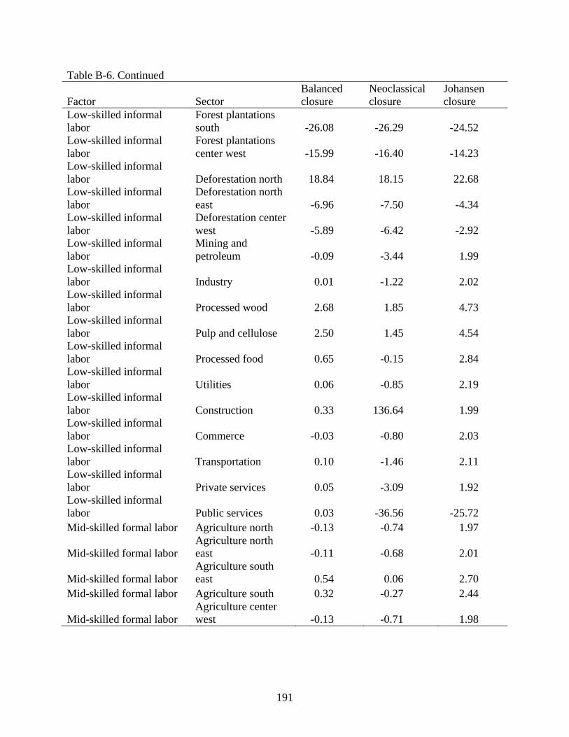
191
Table B-6. Continued
Factor Sector Balanced closure
Neoclassical closure
Johansen closure
Low-skilled informal labor
Forest plantations south -26.08 -26.29 -24.52
Low-skilled informal labor
Forest plantations center west -15.99 -16.40 -14.23
Low-skilled informal labor Deforestation north 18.84 18.15 22.68 Low-skilled informal labor
Deforestation north east -6.96 -7.50 -4.34
Low-skilled informal labor
Deforestation center west -5.89 -6.42 -2.92
Low-skilled informal labor
Mining and petroleum -0.09 -3.44 1.99
Low-skilled informal labor Industry 0.01 -1.22 2.02 Low-skilled informal labor Processed wood 2.68 1.85 4.73 Low-skilled informal labor Pulp and cellulose 2.50 1.45 4.54 Low-skilled informal labor Processed food 0.65 -0.15 2.84 Low-skilled informal labor Utilities 0.06 -0.85 2.19 Low-skilled informal labor Construction 0.33 136.64 1.99 Low-skilled informal labor Commerce -0.03 -0.80 2.03 Low-skilled informal labor Transportation 0.10 -1.46 2.11 Low-skilled informal labor Private services 0.05 -3.09 1.92 Low-skilled informal labor Public services 0.03 -36.56 -25.72 Mid-skilled formal labor Agriculture north -0.13 -0.74 1.97
Mid-skilled formal labor Agriculture north east -0.11 -0.68 2.01
Mid-skilled formal labor Agriculture south east 0.54 0.06 2.70
Mid-skilled formal labor Agriculture south 0.32 -0.27 2.44
Mid-skilled formal labor Agriculture center west -0.13 -0.71 1.98

192
Table B-6. Continued
Factor Sector Balanced closure
Neoclassical closure Johansen closure
Mid-skilled formal labor Forestry north 143.65 142.52 148.80 Mid-skilled formal labor Forestry north east -14.82 -15.10 -13.00 Mid-skilled formal labor Forestry south east -9.40 -9.93 -7.51 Mid-skilled formal labor Forestry south -9.54 -10.06 -7.65 Mid-skilled formal labor Forestry center west -11.18 -11.63 -9.32 Mid-skilled formal labor
Forest plantations north -13.57 -13.98 -11.75
Mid-skilled formal labor
Forest plantations north east -14.40 -14.78 -12.59
Mid-skilled formal labor
Forest plantations south east -20.43 -20.87 -18.78
Mid-skilled formal labor
Forest plantations south -26.08 -26.29 -24.52
Mid-skilled formal labor
Forest plantations center west -15.99 -16.40 -14.23
Mid-skilled formal labor Deforestation north 18.84 18.15 22.68 Mid-skilled formal labor
Deforestation north east -6.96 -7.50 -4.34
Mid-skilled formal labor
Deforestation center west -5.89 -6.42 -2.92
Mid-skilled formal labor
Mining and petroleum -0.09 -3.44 1.99
Mid-skilled formal labor Industry 0.01 -1.22 2.02 Mid-skilled formal labor Processed wood 2.68 1.85 4.73 Mid-skilled formal labor Pulp and cellulose 2.50 1.45 4.54 Mid-skilled formal labor Processed food 0.65 -0.15 2.84 Mid-skilled formal labor Utilities 0.06 -0.85 2.19 Mid-skilled formal labor Construction 0.33 136.64 1.99 Mid-skilled formal labor Commerce -0.03 -0.80 2.03

193
Table B-6. Continued
Factor Sector Balanced closure Neoclassical closure
Johansen closure
Mid-skilled formal labor Transportation 0.10 -1.46 2.11 Mid-skilled formal labor Private services 0.05 -3.09 1.92 Mid-skilled formal labor Public services 0.03 -36.56 -25.72 Mid-skilled informal labor Agriculture north -0.13 -0.74 1.97 Mid-skilled informal labor
Agriculture north east -0.11 -0.68 2.01
Mid-skilled informal labor
Agriculture south east 0.54 0.06 2.70
Mid-skilled informal labor Agriculture south 0.32 -0.27 2.44 Mid-skilled informal labor
Agriculture center west -0.13 -0.71 1.98
Mid-skilled informal labor Forestry north 143.65 142.52 148.80 Mid-skilled informal labor Forestry north east -14.82 -15.10 -13.00 Mid-skilled informal labor Forestry south east -9.40 -9.93 -7.51 Mid-skilled informal labor Forestry south -9.54 -10.06 -7.65 Mid-skilled informal labor Forestry center west -11.18 -11.63 -9.32 Mid-skilled informal labor
Forest plantations north -13.57 -13.98 -11.75
Mid-skilled informal labor
Forest plantations north east -14.40 -14.78 -12.59
Mid-skilled informal labor
Forest plantations south east -20.43 -20.87 -18.78
Mid-skilled informal labor
Forest plantations south -26.08 -26.29 -24.52
Mid-skilled informal labor
Forest plantations center west -15.99 -16.40 -14.23
Mid-skilled informal labor Deforestation north 18.84 18.15 22.68 Mid-skilled informal labor
Deforestation north east -6.96 -7.50 -4.34
Mid-skilled informal labor
Deforestation center west -5.89 -6.42 -2.92

194
Table B-6. Continued
Factor Sector Balanced closure
Neoclassical closure
Johansen closure
Mid-skilled informal labor Mining and petroleum -0.09 -3.44 1.99
Mid-skilled informal labor Industry 0.01 -1.22 2.02 Mid-skilled informal labor Processed wood 2.68 1.85 4.73
Mid-skilled informal labor Pulp and cellulose 2.50 1.45 4.54
Mid-skilled informal labor Processed food 0.65 -0.15 2.84 Mid-skilled informal labor Utilities 0.06 -0.85 2.19 Mid-skilled informal labor Construction 0.33 136.64 1.99 Mid-skilled informal labor Commerce -0.03 -0.80 2.03 Mid-skilled informal labor Transportation 0.10 -1.46 2.11 Mid-skilled informal labor Private services 0.05 -3.09 1.92 Mid-skilled informal labor Public services 0.03 -36.56 -25.72
High-skilled formal labor Agriculture north -0.13 -0.74 1.97
High-skilled formal labor Agriculture north east -0.11 -0.68 2.01
High-skilled formal labor Agriculture south east 0.54 0.06 2.70
High-skilled formal labor Agriculture south 0.32 -0.27 2.44
High-skilled formal labor Agriculture center west -0.13 -0.71 1.98
High-skilled formal labor Forestry north 143.65 142.52 148.80
High-skilled formal labor Forestry north east -14.82 -15.10 -13.00
High-skilled formal labor Forestry south east -9.40 -9.93 -7.51
High-skilled formal labor Forestry south -9.54 -10.06 -7.65
High-skilled formal labor Forestry center west -11.18 -11.63 -9.32

195
Table B-6. Continued
Factor Sector Balanced closure
Neoclassical closure
Johansen closure
High-skilled formal labor
Forest plantations north -13.57 -13.98 -11.75
High-skilled formal labor
Forest plantations north east -14.40 -14.78 -12.59
High-skilled formal labor
Forest plantations south east -20.43 -20.87 -18.78
High-skilled formal labor
Forest plantations south -26.08 -26.29 -24.52
High-skilled formal labor
Forest plantations center west -15.99 -16.40 -14.23
High-skilled formal labor Deforestation north 18.84 18.15 22.68 High-skilled formal labor
Deforestation north east -6.96 -7.50 -4.34
High-skilled formal labor
Deforestation center west -5.89 -6.42 -2.92
High-skilled formal labor Mining and petroleum -0.09 -3.44 1.99 High-skilled formal labor Industry 0.01 -1.22 2.02 High-skilled formal labor Processed wood 2.68 1.85 4.73 High-skilled formal labor Pulp and cellulose 2.50 1.45 4.54 High-skilled formal labor Processed food 0.65 -0.15 2.84 High-skilled formal labor Utilities 0.06 -0.85 2.19 High-skilled formal labor Construction 0.33 136.64 1.99 High-skilled formal labor Commerce -0.03 -0.80 2.03 High-skilled formal labor Transportation 0.10 -1.46 2.11 High-skilled formal labor Private services 0.05 -3.09 1.92 High-skilled formal labor Public services 0.03 -36.56 -25.72 High-skilled informal labor Agriculture north -0.13 -0.74 1.97 High-skilled informal labor Agriculture north east -0.11 -0.68 2.01

196
Table B-6. Continued
Factor Sector Balanced closure
Neoclassical closure
Johansen closure
High-skilled informal labor Agriculture south east 0.54 0.06 2.70 High-skilled informal labor Agriculture south 0.32 -0.27 2.44 High-skilled informal labor
Agriculture center west -0.13 -0.71 1.98
High-skilled informal labor Forestry north 143.65 142.52 148.80 High-skilled informal labor Forestry north east -14.82 -15.10 -13.00 High-skilled informal labor Forestry south east -9.40 -9.93 -7.51 High-skilled informal labor Forestry south -9.54 -10.06 -7.65 High-skilled informal labor Forestry center west -11.18 -11.63 -9.32 High-skilled informal labor
Forest plantations north -13.57 -13.98 -11.75
High-skilled informal labor
Forest plantations north east -14.40 -14.78 -12.59
High-skilled informal labor
Forest plantations south east -20.43 -20.87 -18.78
High-skilled informal labor
Forest plantations south -26.08 -26.29 -24.52
High-skilled informal labor
Forest plantations center west -15.99 -16.40 -14.23
High-skilled informal labor Deforestation north 18.84 18.15 22.68 High-skilled informal labor
Deforestation north east -6.96 -7.50 -4.34
High-skilled informal labor
Deforestation center west -5.89 -6.42 -2.92
High-skilled informal labor Mining and petroleum -0.09 -3.44 1.99 High-skilled informal labor Industry 0.01 -1.22 2.02 High-skilled informal labor Processed wood 2.68 1.85 4.73 High-skilled informal labor Pulp and cellulose 2.50 1.45 4.54 High-skilled informal labor Processed food 0.65 -0.15 2.84

197
Table B-6. Continued
Factor Sector Balanced closure
Neoclassical closure
Johansen closure
High-skilled informal labor Utilities 0.06 -0.85 2.19 High-skilled informal labor Construction 0.33 136.64 1.99 High-skilled informal labor Commerce -0.03 -0.80 2.03 High-skilled informal labor Transportation 0.10 -1.46 2.11 High-skilled informal labor Private services 0.05 -3.09 1.92 High-skilled informal labor Public services 0.03 -36.56 -25.72 Capital Agriculture north -0.13 -0.74 1.97 Capital Agriculture north east -0.11 -0.68 2.01 Capital Agriculture south east 0.54 0.06 2.70 Capital Agriculture south 0.32 -0.27 2.44
Capital Agriculture center west -0.13 -0.71 1.98
Capital Forestry north 143.65 142.52 148.80 Capital Forestry north east -14.82 -15.10 -13.00 Capital Forestry south east -9.40 -9.93 -7.51 Capital Forestry south -9.54 -10.06 -7.65 Capital Forestry center west -11.18 -11.63 -9.32
Capital Forest plantations north -13.57 -13.98 -11.75
Capital Forest plantations north east -14.40 -14.78 -12.59
Capital Forest plantations south east -20.43 -20.87 -18.78
Capital Forest plantations south -26.08 -26.29 -24.52
Capital Forest plantations center west -15.99 -16.40 -14.23
Capital Deforestation north 18.84 18.15 22.68
Capital Deforestation north east -6.96 -7.50 -4.34
Capital Deforestation center west -5.89 -6.42 -2.92
Capital Mining and petroleum -0.09 -3.44 1.99 Capital Industry 0.01 -1.22 2.02 Capital Processed wood 2.68 1.85 4.73

198
Table B-6. Continued
Factor Sector Balanced closure
Neoclassical closure
Johansen closure
Capital Pulp and cellulose 2.50 1.45 4.54 Capital Processed food 0.65 -0.15 2.84 Capital Utilities 0.06 -0.85 2.19 Capital Construction 0.33 136.64 1.99 Capital Commerce -0.03 -0.80 2.03 Capital Transportation 0.10 -1.46 2.11 Capital Private services 0.05 -3.09 1.92 Capital Public services 0.03 -36.56 -25.72 Agricultural land north Agriculture north -0.17 -0.77 1.94 Agricultural land north
Forest plantations north -0.17 -0.77 1.94
Agricultural land north east Agriculture north east -0.38 -0.94 1.73 Agricultural land north east
Forest plantations north east -0.38 -0.94 1.73
Agricultural land south east Agriculture south east -6.79 -7.26 -4.81 Agricultural land south east
Forest plantations south east -6.79 -7.26 -4.81
Agricultural land south Agriculture south -1.81 -2.37 0.27 Agricultural land south
Forest plantations south -1.81 -2.37 0.27
Agricultural land center west
Agriculture center west -0.17 -0.75 1.94
Agricultural land center west
Forest plantations center west -0.17 -0.75 1.94
Forestland north Forestry north -64.47 -64.63 -63.72 Forestland north Deforestation north -64.47 -64.63 -63.72 Forestland north east Forestry north east -14.25 -14.55 -12.37
Forestland north east Deforestation north east -14.25 -14.55 -12.37
Forestland southeast Forestry south east -9.40 -9.93 -7.51 Forestland south Forestry south -9.54 -10.06 -7.65 Forestland center west Forestry center west -11.14 -11.59 -9.27 Forestland center west
Deforestation center west -11.14 -11.59 -9.27

199
Table B-7. Percent change in level of domestic activity Sector Balanced closure Neo classical closure Johansen closure Agriculture north 0.00 0.00 0.00 Agriculture north east 0.01 0.01 0.01 Agriculture south east 0.19 0.19 0.19 Agriculture south 0.13 0.12 0.13 Agriculture center west 0.01 0.01 0.01 Forestry north 24.68 24.68 24.68 Forestry north east -0.02 -0.02 -0.03 Forestry south east 0.00 0.00 0.00 Forestry south 0.00 0.00 0.00 Forestry center west -0.01 -0.01 -0.01 Forest plantations north -0.56 -0.56 -0.56 Forest plantations north east -0.62 -0.61 -0.62 Forest plantations south east -2.40 -2.41 -2.41 Forest plantations south -3.71 -3.67 -3.71 Forest plantations center west -1.29 -1.28 -1.29 Deforestation north 1.20 1.20 1.20 Deforestation north east 0.14 0.14 0.15 Deforestation center west 0.09 0.09 0.11 Mining and petroleum 0.00 0.00 0.00 Industry 0.00 0.00 0.00 Wood processing 0.00 0.00 0.00 Pulp and paper 0.00 0.00 0.00 Food processing 0.00 0.00 0.00 Utilities 0.00 0.00 0.00 Construction 0.00 0.00 0.00 Commerce 0.00 0.00 0.00 Transportation 0.00 0.00 0.00 Private services 0.00 0.00 0.00 Public services 0.00 0.00 0.00

200
Table B-8. Percent change in quantity of factor demand by industry
Sector Factor Balanced closure
Neo classical closure
Johansen closure
Agriculture north Agricultural land north 0.01 0.01 0.01
Forest plantations north -2.84 -2.82 -2.84
Agriculture north east Agricultural land north east 0.06 0.06 0.06
Forest plantations north east -2.99 -2.96 -2.99
Agriculture south east Agricultural land south east 1.83 1.84 1.84
Forest plantations south east -3.11 -3.12 -3.12
Agriculture south Agricultural land south 0.52 0.51 0.52
Forest plantations south -5.52 -5.47 -5.52 Agriculture center west
Agricultural land center west 0.01 0.01 0.01
Forest plantations center west -3.39 -3.38 -3.40 Forestry north Forest land north 46.97 46.97 46.97 Deforestation north 6.22 6.22 6.28 Forestry north east Forest land north east -0.13 -0.13 -0.14 Deforestation north east 0.41 0.40 0.44 Forestry south east Forest land south east 0.00 0.00 0.00 Forestry south Forest land south 0.00 0.00 0.00
Forestry center west Forest land center west -0.01 -0.01 -0.01
Deforestation center west 0.29 0.28 0.34

201
Table B-9. Percent change in quantity of sales
Balanced closure
Neoclassical closure
Johansen closure
Balanced closure
Neoclassical closure
Johansen closure
Good or service
Domestic sales
Domestic sales
Domestic sales Exports Exports Exports
Agriculture 0.05 0.09 0.06 0.31 0.04 0.22 Forestry 1.95 1.96 1.95 14.55 14.17 14.45 Deforestation 0.84 0.84 0.85 0.00 0.00 0.00 Mining and petroleum 0.00 0.00 0.00 0.00 0.00 0.00 Industrial 0.01 0.00 0.00 -0.04 0.02 -0.02 Processed wood 0.00 0.00 0.00 0.00 0.00 0.00 Pulp and cellulose 0.00 0.00 0.00 0.00 0.00 0.00 Processed food 0.02 0.09 0.06 -0.07 -0.46 -0.30 Utilities 0.00 0.00 0.00 0.00 0.00 0.00 Construction 0.00 0.15 0.00 -0.09 -23.44 0.00 Commerce 0.00 0.00 0.00 0.00 0.00 0.00 Transportation 0.00 -0.01 0.00 -0.08 0.33 -0.05 Private services 0.00 -0.01 0.00 -0.04 0.41 0.03 Public services 0.00 0.00 0.00 0.00 0.00 0.00

202
Table B-10. Percent change in quantity of composite goods supply Activity Balanced closure Neo classical closure Johansen closure Agriculture 0.03 0.09 0.05 Forestry 0.37 0.43 0.38 Deforestation 0.84 0.84 0.85 Mining and petroleum 0.00 0.00 0.00 Industrial 0.01 -0.01 0.01 Processed wood 0.00 0.00 0.00 Pulp and cellulose 0.00 0.00 0.00 Processed food 0.02 0.10 0.07 Utilities 0.00 0.00 0.01 Construction 0.00 0.32 0.00 Commerce 0.00 0.00 0.00 Transportation 0.00 -0.01 0.00 Private services 0.01 -0.07 -0.01 Public services 0.00 0.00 0.00

203
LIST OF REFERENCES
About UNFF. (2006). United Nations Forum on Forests [UNFF]. Home page. Retrieved July 2, 2007, from http://www.un.org/esa/forests/
Ahrens, S. (2003). O “novo” código florestal brasileiro: conceitos jurídicos fundamentais. Paper
presented at the VIII Congresso Florestal Brasileiro, São Paulo, Brasil, August 25-28. Retrieved June 16, 2007, from http://www.ambientebrasil.com.br/florestal/download/SAhrensCodigoFlorestal.pdf
Alavalapati, J. R. R., Adamowicz, W. L., & White, W. A. (1998a). A comparison of economic
impact assessment methods: the case of forestry developments in Alberta. Canadian Journal of Forest Research, 28, 711-719.
Alavalapati, J. R. R., Adamowicz, W. L., & White, W. A. (1999). Random variables in Forest
policy: a systematic sensitivity analysis using CGE models. Journal of Forest Economics, 5(2), 321-335.
Alavalapati, J. R. R., White, B., Jagger, P., & Wellstead, A. (1998b). Effect of land use
restrictions on the economy of Alberta: a computable general equilibrium analysis. Canadian Journal of Regional Science, 19(3), 349-365.
Alavalapati, J. R. R., Percy, M. B., & Luckert, M. K. (1997). A computable general equilibrium
analysis of a stumpage price increase policy in British Columbia. Journal of Forest Economics, 3(2), 143-169.
Albert, B. (1992). Indian lands, environmental policy and military geopolitics in the development
of the Brazilian Amazon: the case of the Yanomami. Development and Change, 23, 35-70. Retrieved July 2, 2007 from http://horizon.documentation.ird.fr/exl-doc/pleins_textes/pleins_textes_5/b_fdi_31-32/35009.pdf
Alonso, A., Costa, V., & Maciel, D. (2005). The formation of the Brazilian environmental
movement. Institute of Development Studies [IDS] Working Paper 259. Brighton: IDS. Retrieved December 9, 2007, from http://www.drc-citizenship.org/docs/publications/citizens_and_science/WP/Wp259.pdf
Amacher, G. S. (2006). Corruption: a challenge for economists interested in forest policy design.
Journal of Forest Economics, 12(2), 85-89. Annabi, N., Cockburn, J., & Decaluwé, B. (2006). Functional forms and parameterization of
CGE models. Poverty and Economic Policy, MPIA Working Paper 2006-04. Retrieved December 9, 2007, from: http://papers.ssrn.com/sol3/papers.cfm?abstract_id=897758
Arndt, C., & Pearson, K. R. (1998). How to carry out systematic sensitivity analysis via
Gaussian Quadrature and GEMPACK. GTAP Technical Paper No. 3. Retrieved July 23, 2008, from: https://www.gtap.agecon.purdue.edu/resources/res_display.asp?RecordID=474

204
Associação Brasileira de Celulose e Papel [BRACELPA]. (2005). Statistical forest report. GT reforestation and correlates. Retrieved December 9, 2007, from http://www.ipef.br/estatisticas/relatorios/Bracelpa-Relatorio_Estatistico_Florestal-2005-Eng.pdf
Associação Brasileira de Celulose e Papel [BRACELPA]. (2003). Relatório Estatístico Florestal
-2003. GT- Reflorestamento e Correlatos. Retrieved April 15, 2008, from www.ipef.br/estatisticas/relatorios/Bracelpa-Relatorio_Estatistico_Florestal-2003.pdf
Bandara, J. S. (1991). Computable general equilibrium models for development policy analysis
in LDCs. Journal of Economic Surveys, 5(1), 3-69. Barreto, P., Amaral, P., Vidal, E., & Uhl, C. (1998). Costs and benefits of forest management for
timber production in eastern Amazonia. Forest Ecology and Management, 108, 9-26. Brito, B., Barreto, P., & Rothman, J. (2005). Brazil’s new Environmental Crimes Law: an
analysis of its effectiveness in protecting Amazonian forests. Belém: Instituto do Homem e meio ambiente da Amazônia. Retrieved April 1, 2008, from http://www.illegal-logging.info/uploads/crimes_law_brito.pdf
Brito, B. & Barreto, P. (2006). Enforcement against illegal logging in the Brazilian Amazon.
Retrieved April 1, 2008, from http://www.imazon.org.br/publicacoes/publicacao.asp?id=478
Barreto, P., Souza, C., Noguerón, R., Anderson, & A., Salomão, R. (2006). Human pressure on
the Brazilian Amazon forests. Belém: World Resources Institute. Retrieved April 1, 2008, from http://www.wri.org/publication/human-pressure-brazilian-amazon-forests
Benjamin, A. H. V. (2000). A proteção das florestas Brasileiras: ascensão e queda do Código
Florestal. Paper presented at the invitation of the Secretaria de Coordenação da Amazônia, Brasília, Brazil, January 17, 2000. Retrieved June 16, 2007, from http://bdjur.stj.gov.br/dspace/handle/2011/8962
Brazil environment chief a former rubbertapper. (2002, December 11). Environment News
Service. Retrieved July 4, 2007, from http://www.ens-newswire.com/ens/dec2002/2002-12-11-01.asp
Brazil farmers bury activist nun. (2005b, February 16). BBC News, Americas. Retrieved June 16,
2007 from http://news.bbc.co.uk/2/hi/americas/4266959.stm Brazilian Government press release on the actions taken by the Ministry of Environment to
dismantle gang acting in Mato Grosso for 14 years. (2005, June 2). Consulate General of Brazil in San Francisco. Retrieved June 16, 2007, from http://www.brazilsf.org/brazil_press6.htm

205
Buetre, B., Rodriguez, & G., Pant, H. (2003). Data issues in general equilibrium modelling. Australian Bureau of Agricultural and Resource Economics Conference Paper 03.2. Presented at 47th Australian Agricultural and Resource Economics Society Conference in Freemantle, Western Australia, 11-14 February 2003, pp1-17. Retrieved April 15, 2008, from http://www.aares.info/files/2003_buetre.pdf
Callister, D. J. (1999). Corrupt and illegal activities in the forestry sector: current
understandings, and implications for World Bank Forest Policy. Draft for Discussion. The World Bank Group. Forest Policy Implementation Review and Strategy Development: Analytical Studies. Retrieved April 1, 2008, from http://lnweb18.worldbank.org/eap/eap.nsf/Attachments/FLEG_OB6/$File/OB+6+FPR+Paper+-+Illegal+Actions+-+Debra+Callister.pdf.
Cattaneo, A. (1999). Technology, migration, and the last frontier: a general equilibrium analysis
of environmental feedback effects on land use patterns in the Brazilian Amazon. Unpublished doctoral dissertation, John Hopkins University, Baltimore, USA.
Cattaneo, A. (2001). Deforestation in the Brazilian Amazon: comparing the impacts of
macroeconomic shocks, land tenure, and technological change. Land Economics 77(2), 219-240.
Cattaneo, A. (2002). Balancing agricultural development and deforestation in the Brazilian
Amazon. International Food Policy Research Institute Research Report 129. Washington, D.C.: IFPRI. Retrieved April 15, 2008, from http://www.ifpri.org/pubs/abstract/abstr129.htm
Celentano, D., & Veríssimo, A. (2007). O avanço da fronteira na Amazônia: do boom ao
colapso. Belém: IMAZON. Retrieved April 15, 2008, from www.imazon.org.br/publicacoes/publicacao.asp?id=512
Chadwick, B. P. (2000). Democratic environments: democratization and the search for
sustainable development in Brazil. Unpublished doctoral dissertation, Columbia University, New York City, USA.
Contreras-Hermosilla, A. (2002). Law compliance in the forestry sector- an overview. World
Bank Institute Working Paper. Washington, D.C.: World Bank. Retrieved March 1, 2008, from http://www.illegal-logging.info/item_single.php?item=document&item_id=25&approach_id=2
Contreras-Hermosilla, A., Doornbosch, R., & Lodge, M. (2007). The economics of illegal
logging and associated trade. Organisation for Economic Co-operation and Development. Round Table on Sustainable Development, SG/SD/RT. Retrieved April 13, 2008, from http://www.oecd.org/LongAbstract/0,3425,en_39315735_39313128_39348797_119684_1_1_1,00.html

206
Dee, P. S. (1991). Modeling steady state forestry in computable general equilibrium context. Working Paper No. 91/8. Canberra: National Centre for Development Studies.
Dewatripont, M., & Michel, G. (1987). On closure rules, homogeneity and dynamics in applied
general equilibrium models. Journal of Development Economics, 26(1), 65-76. Dixon, P. B., Parmenter, B. R. (1996). Computable general equilibrium modeling for policy
analysis and forecasting. In H. M. Amman, D. A. Kendrick & J. Rust (Eds.), Handbook of Computational Economics, Volume I, Elsevier Science.
Dixon, P. B., Parmenter, B. R., Powell, A. A., Wilcoxen, P.J. (1992). Notes and problems in
applied general equilibrium economics. In C. J. Bliss & M. D. Intriligator (Eds.), Advanced textbooks in economics, Volume 32. Amsterdam: Elsevier Science B.V.
Drummond, J., & Barros-Platiau, A. F. (2006). Brazilian environmental laws and policies, 1934-
2002: a critical overview. Law & Policy, 28(1), 83-108. Dufournaud, C. M., Jerrett, M., Quinn, J. T., Maclaren, V. (2000). Economy-wide effects of
forest policies: a general equilibrium assessment from Vietnam. Land Economics, 76(1), 15-27.
Food and Agriculture Organization of the United Nations [FAO]. (1996). Agro-ecological
zoning guidelines. FAO Soils Bulletin 73. Soil Resources, Management and Conservation Service. FAO Land and Water Development Division. Rome: FAO. Retrieved July 20, 2008, from http://www.fao.org/docrep/w2962e/w2962e00.htm#P-2
Food and Agriculture Organization of the United Nations. (2005). Best practices for improving
law compliance in the forestry sector. FAO Forestry Paper 145. Rome: FAO. Retrieved May 25, 2008, from http://www.fao.org/docrep/008/a0146e/a0146e00.HTM
FAOSTAT. (2005). ForestSTAT. Online forest sector statistical database. Retrieved December 9,
2007, from http://faostat.fao.org/site/381/default.aspx Fearnside, P. M., & Barbosa R. I. (2004). Accelerating deforestation in Brazilian Amazonia:
towards answering open questions. Environmental Conservation, 31(1), 7-10. Figueiredo, C. C. M. (2007). From paper parks to real conservation: case studies of national
park management effectiveness in Brazil. Unpublished doctoral dissertation, The Ohio State University, Columbus, USA.
Fortin, B., Marceau, N., & Savard, L. (1997). Taxation, wage controls and the informal sector.
Journal of Public Economics, 66, 293-312. Gan, J. (2004). Effects of China’s WTO accession on global forest product trade. Forest Policy
and Economics, 6, 509-519.

207
Gan, J. (2005). Forest certification costs and global forest product markets and trade: a general equilibrium analysis. Canadian Journal of Forest Research, 35(7), 1731-1743.
General Algebraic Modeling System. Welcome to the GAMS home page. Retrieved April 15,
2008, from http://www.gams.com/ Gibson, B. (2004). The transition to a globalized economy: poverty, human capital and the
informal sector in a structuralist CGE model. Journal of Development Economics, 78, 60-94.
Glantz, M. H., Brook, A. T. & Parisi, P. (1997). Rates and processes of Amazon deforestation.
Environmental and Societal Impacts Group, National Center for Atmospheric Research. Retrieved June 12, 2008, from http://www.ccb.ucar.edu/rates/processes.html
Governo cria 5.2 milhões de hectares de áreas protegidas e interdita outros 8,2 milhões para
estudos. (2005a, February 18). Instituto Socioambiental, Noticias socioambientais. Retrieved June 16, 2007, from http://www.socioambiental.org/nsa/detalhe?id=1924
Governo cria UCs e distrito florestal no entorno da BR-163 (Cuiabá-Santarém). (2006b,
February 14). Instituto Socioambiental, Noticias socioambientais. Retrieved June 16, 2007, from http://www.socioambiental.org/nsa/detalhe?id=2189
Governo Lula acaba se complicando no conflito de Novo Progresso. (2005c, February 15).
Instituto Socioambiental, Noticias socioambientais. Retrieved June 16, 2007, from http://www.socioambiental.org/nsa/detalhe?id=1920
Grileiros aterrorizam comunidades riberinhas na Terrra do Meio (PA). (2005b, January 31). Instituto Socioambiental, Noticias socioambientais. Retrieved June 16, 2007, from: http://www.socioambiental.org/nsa/detalhe?id=1912
Guevara, R. (2003). Making concessions in Brazil. International Tropical Timber Organization Tropical Forest Update, 13/3. Retrieved November 12, 2007, from http://219.127.136.74/live/Live_Server/311/tfu.2003.03(03).e.pdf
Gutierrez-Velez, V. H., & MacDicken, K. (2008). Quantifying the direct social and governmental costs of illegal logging in the Bolivian, Brazilian, and Peruvian Amazon. Forest Policy and Economics, 10, 248-256.
Hirakuri, S. R. (2003). Can law save the forests? Lessons from Finland and Brazil. Bogor:
Center for International Forestry Research. Retrieved June 16, 2007, from http://www.cifor.cgiar.org/publications/pdf_files/Books/Law.pdf
Instituto Brasileiro de Geografia e Estatística [IBGE]. (1996). Censo agropecuário. Retrieved April 1, 2008, from http://www.ibge.gov.br/home/estatistica/economia/agropecuaria/censoagro/1995_1996/default.shtm

208
Instituto Brasileiro de Geografia e Estatística [IBGE]. (2003). Censo demográfico- 2000. Rio de Janeiro: IBGE. Retrieved April 15, 2008, from http://www.ibge.gov.br/home/estatistica/populacao/default_censo_2000.shtm
Instituto Brasileiro de Geografia e Estatística [IBGE]. (2004a). Sistemas de contas nacionais-
Brasil 2003. Rio de Janeiro: IBGE. Retrieved April 15, 2008, from http://www.ibge.gov.br/home/estatistica/economia/contasnacionais/referencia1985/2003/contasnacionais2003.pdf
Instituto Brasileiro de Geografia e Estatística [IBGE]. (2004b). Pesquisa nacional por amostra de domicílios- 2003. Rio de Janeiro: IBGE. Retrieved April 15, 2008, from http://www.ibge.gov.br/home/estatistica/populacao/trabalhoerendimento/pnad2003/default.shtm
Instituto Brasileiro de Geografia e Estatística [IBGE]. (2004c). Produção da extração vegetal e da silvicultura – 2003. Rio de Janeiro: IBGE. Retrieved April 15, 2008, from http://www.ibge.gov.br/home/estatistica/economia/pevs/2003/default.shtm
Instituto Brasileiro de Geografia e Estatística [IBGE]. (2005). Contas regionais do Brasil- 2003.
Rio de Janeiro: IBGE. Retrieved April 15, 2008, from http://www.ibge.gov.br/home/estatistica/economia/contasregionais/2003/default.shtm
Instituto Brasileiro de Geografia e Estatística [IBGE]. (2007a). Produção da extração vegetal e
da silvicultura – 2006. Rio de Janeiro: IBGE. Retrieved April 15, 2008, from http://www.ibge.gov.br/home/estatistica/economia/pevs/2006/pevs2006.pdf
Instituto Brasileiro de Geografia e Estatística [IBGE]. (2007b). Pesquisa de orçamentos
familiares 2002-2003. Rio de Janeiro: IBGE. Retrieved April 15, 2008, from http://www.ibge.gov.br/home/estatistica/populacao/trabalhoerendimento/pnad2003/default.shtm
Instituto Brasileiro de Geografia e Estatística [IBGE]. (2007c). Censo agropecuário. Rio de
Janeiro: IBGE. Retrieved April 15, 2008, from http://www.ibge.gov.br/home/estatistica/economia/agropecuaria/censoagro/2006/default.shtm
Instituto Nacional de Pesquisas Espaciais [INPE]. (2007). Projeto PRODES- monitoramento da
floresta Amazônica Brasileira por satélite. Retrieved December 9, 2007, from: http://www.obt.inpe.br/prodes/index.html
Ioris, E. M. (2005). A forest of disputes: struggles over spaces, resources, and social identities in
Amazonia. Unpublished doctoral dissertation, University of Florida, Gainesville, USA.

209
Jaeger, M. (2006). Brazil: o país do future? Economic scenarios for the next 15 years. Current Issues. Frankfurt: Deutsche Bank Research. Retrieved June 15, 2008, from http://129.35.230.60/PROD/DBR_INTERNET_EN-PROD/PROD0000000000199361.PDF
Kaimowitz, D. & Angelsen, A. (1998). Economic models of tropical deforestation. Bogor:
Center for International Forestry Research. Retrieved June 10, 2008, from http://www.cifor.cgiar.org/publications/pdf_files/books/model.pdf
Kelley, B. (1994). The informal sector and the macroeconomy: a computable general equilibrium
approach for Peru. World Development, 22(9), 1393-1411. Kengen, S. (2001). A política florestal Brasileira: uma perspectiva histórica. Paper presented at
1º Simpósio Ibero-Americano de Gestão e Economia Florestal, Porto Seguro, Brazil, July 4-7, 2001. Instituto de Pesquisas e Estudos Florestais. Retrieved May 4, 2007, from http://www.ipef.br/eventos/siagef2001/programacao.html
Kolk, A. (1996). Forests in international environmental politics: international organisations, NGOs and the Brazilian Amazon. Utrecht: International.
Kraev, E. (2003). Modelling macroeconomic and distributional impacts of stabilization and
adjustment packages: current literature and challenges. Center for Economic Policy Analysis [CEPA], CEPA Working Paper 2003-6, 1-50.
Laurance, W. F., Albernaz, A. K. M., & da Costa, C. (2002). O desmatamento está se acelerando
na Amazônia Brasileira? Biota Neotropica, 2(1), 1-9. Retrieved June 16, 2007, from http://lcluc.umd.edu/products/LBA_page/files_fr_2_25_email/Laur2001_Is_Defor_Portg.pdf
Lele, U., Viana, V., Veríssimo, A., Vosti, S., Perkins, K., & Husain, S. A. (2000). Brazil, forests
in the balance: challenges of conservation with development. Evaluation Country Case Study Series. Washington, D.C.: The World Bank. Retrieved April 1, 2008, from http://lnweb18.worldbank.org/oed/oeddoclib.nsf/DocUNIDViewForJavaSearch/D985594AF1F1DFB185256970007C1ACC
Lentini, M., Pereira, D., Celentano, D., & Pereira, R. (2005a). Fatos florestais da Amazônia
2005. Belém: IMAZON. Retrieved April 15, 2008, from http://www.imazon.org.br/publicacoes/publicacao.asp?id=377
Lentini, M., Veríssimo, A., & Pereira, D. (2005b). A expansão madeireira na Amazônia. O
Estado da Amazônia No. 2, May, 2005. Belém: IMAZON. Retrieved April 15, 2008, from http://www.imazon.org.br/downloads/index.asp?categ=1
Leonel, M. H. (2005). Forest plantations in Brazil. Paper presented at the forty-sixth session of
the FAO Advisory Committee on Paper and Wood Products, Vancouver, Canada, May 31, 2005. Retrieved June 16, 2007, from http://www.fao.org/forestry/media/10549/1/0/

210
Levantis, T., & Fairhead, L. (2004). PNGGEM, ABARE’s model of the economy of Papua New Guinea. Australian Government, Australian Bureau of Agricultural and Resource Economics.
Lima, E., Merry, F., Nepstad, D., Amacher, G., Azevedo-Ramos, C., Resque, F., & Lefebvre, P.
(2006). Searching for sustainability: forest policies, smallholders and the Trans-Amazon Highway. Environment, 48, 26-37.
Loayza, N. V. (1997). The economics of the informal sector. A simple model and some empirical
evidence from Latin America. Washington, D.C.: The World Bank. Retrieved May 20, 2008, from http://econ.worldbank.org/external/default/main?pagePK=64165259&piPK=64165421&theSitePK=469372&menuPK=64216926&entityID=000009265_3970619111006
Lofgren, H., Harris, R.L., Robinson, S., Thomas, M., & El-Said, M. (2002). A standard
computable general equilibrium (CGE) model in GAMS. International Food Policy Research Institute, Microcomputers in Policy Research 5. Washington, D.C.: IFPRI. Retrieved July 2, 2007, from http://www.ifpri.org/pubs/microcom/5/mc5.pdf
Lopez, A. (2000). Environmental change, social conflicts and security in the Brazilian Amazon:
exploring the links. Doctoral dissertation, University of Oslo, Blindern, Norway. Retrieved July 2, 2007, from http://www.statsvitenskap.uio.no/fag/polit/disputas/fulltxt/lopez.pdf
Lula: fourth time lucky. (2002, October 28). BBC News World Edition. Retrieved July 4, 2007,
from http://news.bbc.co.uk/2/hi/americas/2367851.stm Macqueen, D., Grieg-Gran, M., Lima, E., MacGregor, J., Merry, F., Prochnick, V., Scotland, N.,
Smeraldi, R., & Young, C. (2003). Growing timber exports: the Brazilian tropical timber industry and international markets. Edinburgh: International Institute for Environment and Development. Retrieved October 14, 2007, from http://www.iied.org/pubs/display.php?n=2&l=2&a=R%20Smeraldi&x=Y
Mahar, D. J. (1989). Government policies and deforestation in Brazil's Amazon Region.
Washington, D.C.: The World Bank. Marquesini, M., & Edwards, G. (2001). The Santarém five & illegal logging- a case study.
Greenpeace Amazon Expedition, October, 2001. Retrieved May 1, 2008, from http://archive.greenpeace.org/forests/forests_new/html/content/docs.html
Marty, R. J. (1986). The economics of forestry- forestry and economic development. In G. W.
Sharpe, C. W. Hendee, & W. Sharpe (Eds.), Introduction to Forestry. New York: McGraw-Hill.
McKitrick, R. R. (1998). The econometric critique of computable general equilibrium modeling:
the role of functional forms. Economic Modeling, 15, 543-573.

211
Merry, F. D., & Amacher, G. S. (2005). Forest taxes, timber concessions, and policy choices in the Amazon. Journal of Sustainable Forestry, 20(2), 15-44.
Mery, G., Kengen, S. & Luján, C. (2001). Forest-based development in Brazil, Chile and
Mexico. In M. Palo, J. Uusivuori, & G. Mery (Eds.), World Forests, Markets and Policies. Dordecht: Kluwer Academic Publishers.
Ministério do Meio Ambiente [MMA]. (2001). The National Forest Program- PNF. Brasília:
Ministério do Meio Ambiente/ Serviço Florestal Brasileiro/Diretoria de Florestas. Retrieved June 29, 2007, from http://www.brasilemb.org/environment/pnfing.pdf
Ministério do Meio Ambiente [MMA]. (2005). Nota de esclarecimento sobre Projeto de Lei
4776/2005 sobre Gestão de Florestas Publicas. Ministério do Meio Ambiente, Secretaria de Biodiversidade e Florestas and Diretoria do Programa Nacional de Florestas: Brasília. Retrieved May 25, 2008, from http://www.amazonia.org.br/guia/detalhes.cfm?id=154716&tipo=6&cat_id=87&subcat_id=1
Ministério do Meio Ambiente [MMA]. (2008a). Portal nacional de gestão florestal. Sistema de
Monitoramento e Controle dos Recursos e Produtos Florestais [SISPROF]. Retrieved October 14, 2007, from http://www.mma.gov.br/index.php?ido=conteudo.monta&idEstrutura=113
Ministério do Meio Ambiente [MMA]. (2008b). Evolução da área com florestas plantadas.
Programa Nacional de Florestas. Ministério de Minas e Energia. (No date). World expansion- 1970 to 2020. Retrieved June 15,
2008, from www.mme.gov.br/html/ben2004/Ingles/world_energy.pdf Mittermeier, R. A., da Fonseca, G. A. B., Rylands, A. B., & Brandon, K. (2005). A brief history
of biodiversity conservation in Brazil. Conservation Biology, 19(3), 601-607. Morandi, L., Reis, E. (2004). Estoque de capital fixo no Brasil, 1950-2002. Anais do XXXII
Encontro Nacional de Economia, ANPEC - Associação Nacional dos Centros de Pósgraduação em Economia. Retrieved May 25, 2008, from http://ideas.repec.org/p/anp/en2004/042.html
Morton, D. (2005, September/October). Looking at Lula- Brazil’s Amazon deforestation worsens
despite a “Green” President. EMagazine.com, 16(5), 14-16. Retrieved October 14, 2007, from http://www.emagazine.com/view/?2839
Murder prompts Brazil Amazon curb. (2005a, February 18). BBC News, Americas. Retrieved
June 16, 2007, from: http://news.bbc.co.uk/1/hi/world/americas/4275781.stm#

212
Nepstad, D., Schwartzman, S., Bamberger, B., Santilli, M., Ray, D., Schlesinger, P., Lefebvre, P., Alencar, A., Prinz, E., Fiske, G., & Rolla, A. (2006). Inhibition of Amazon deforestation and fire by parks and indigenous lands. Conservation Biology, 20(1), 65-73.
Ondro, W. J., Couto, L., & Betters, D. R. (1995). The status and practice of forestry in Brazil in
the early 1990s. The Forestry Chronicle, 71(1), 106-119. Organisation for Economic Co-operation and Development [OECD]. (2006). Brazil. OECD
economic surveys. Volume 2006/18. Paris: OECD. Retrieved May 25, 2008, from http://www.oecd.org/document/62/0,3343,fr_2649_34571_37661246_1_1_1_1,00.html
Patusco, J. A. M. (2002). Long-term planning. Economy & Energy, No. 35. Retrieved June 15,
2008, from http://ecen.com/eee35/Long%20Term%20Planning.htm Pereira, M. P., Shoven, J. B. (1988). Survey of dynamic computational general equilibrium
models for tax policy evaluation. Journal of Policy Modeling, 10(3), 401-436. Persson, A. & Munasinghe, M. (1995). Natural resource management and economywide policies
in Costa Rica: a computable general equilibrium (CGE) modeling approach. The World Bank Economic Review, 9(2), 259-285.
Pinedo-Vasquez, M., Zarin, D. J., Coffey, K., Padoch, C., & Rabelo, F. (2001). Post boom
logging in Amazonia. Human Ecology, 29(2), 219-239. Presidência da Republica. (2004). Plano de ação para prevenção e controle do desmatamento na
Amazônia Legal. Brasília: Grupo Permanente de Trabalho Interministerial para a Redução dos Índices de Desmatamento da Amazônia Legal. Retrieved June 16, 2007, from http://www.planalto.gov.br/casacivil/desmat.pdf
Purusshothaman, R. (no date). The BRICs’ path to 2050: A dramatically different global
economy. Goldman Sachs. Retrieved June 15, 2008, from http://coursenligne.sciences-po.fr/2005_2006/gouvernance/braga/cours_1_brics.pdf
Quem chega primeiro na Amazônia: o estado ou o grileiro? (2006a, November). Instituto
Socioambiental, Noticias socioambientais. Retrieved June 16, 2007, from http://www.socioambiental.org/esp/desmatamento/site/grilagem
Reydon, B. P., & Plata, L. A. (2000). Evolução recente do preço da terra rural no Brasil e os
impactos do Programa da Cédula da Terra. Brasília: Núcleo de Educação a Distancia [NEAD].
Rhodes, W. M., Allen, E. P., & Callahan, M. (2006). Illegal logging: a market-based analysis of
trafficking in illegal timber. Research report submitted to the U.S. Department of Justice. Contract # 2004 TO 164. May 31, 2006. Retrieved April 18, 2008, from http://www.ncjrs.gov/pdffiles1/nij/grants/215344.pdf

213
Robinson, S., Cattaneo, A., & El-Said, M. (2001). Updating and estimating a social accounting matrix using cross entropy methods. Economic Systems Research, 13(1), 47-64.
Robinson, S., & El-Said, M. (2000). GAMS code for estimating a social accounting matrix
(SAM) using cross entropy (CE) methods. International Food Policy Research Institute, Trade and Macroeconomics Discussion Paper No. 64. Washington, D.C.: IFPRI. Retrieved June 16, 2007, from http://www.ifpri.org/divs/tmd/dp/papers/tmdp64.pdf
Robinson, S., & Thurlow, J. (no date). A recursive dynamic computable general equilibrium
(CGE) model: extending the standard IFPRI static model. Rohter, L. (2002, September 23). A Brazilian campaign that is all about the jungle. The New
York Times. Retrieved October 14, 2007, from http://query.nytimes.com/gst/fullpage.html?res=9506E7D91739F930A1575AC0A9649C8B63&n=Top/News/Science/Topics/Environment
Rose, A. (1995). Input-output economics and computable general equilibrium models. Structural
Change and Economic Dynamics, 6, 295-304. Rylands, A. B., & Brandon, K. (2005). Brazilian protected areas. Conservation Biology, 19(3),
612-618. Seneca Creek Associates & Wood Resources. (2004). “Illegal” logging and global wood
markets: the competitive impacts on the U.S. wood products industry. Retrieved April 18, 2008, from http://www.afandpa.org/Content/NavigationMenu/News_Room/Papers_Reports1/AFPAIllegalLoggingReportFINAL2.pdf
Serviço Florestal Brasileiro [SFB]. (2007a). Gestão das florestas públicas- relatório 2006.
Brasília: Ministério do Meio Ambiente. Retrieved June 16, 2007, from: http://www.amazonia.org.br/arquivos/240311.pdf
Serviço Florestal Brasileiro [SFB]. (2007b). Distribuição de florestas publicas federais em identificação por destino. Retrieved April 15, 2008, from http://www.mma.gov.br/index.php?ido=conteudo.monta&idEstrutura=95&idConteudo=6098
Serviço Florestal Brasileiro [SFB]. (2007c). Plano anual de outorga florestal. Brasília:
Ministério do Meio Ambiente. Retrieved April 15, 2008, from http://www.ibama.gov.br/cenaflor/download.php?id_download=32
Shoven, J. B. & Whalley, J. (1984). Applied general-equilibrium models of taxation and
international trade: an introduction and survey. Journal of Economic Literature, 22(3), 1007-1051.
Silva, M. (2005). The Brazilian protected areas program. Conservation Biology, 19 (3), 608-611.

214
Siqueira, C. F. A., & Nogueira, J. M. (2004). O Novo Código Florestal e a reserva legal: do preservacionismo desumano ao conservacionismo politicamente correto. Anais do XLII Encontro Brasileiro de Economia e Sociologia Rural- Encontro da SOBER, Cuiabá, 2004. Retrieved June 16, 2007, from http://www.unb.br/face/eco/jmn/trabalhos/2004/novocodigoflorestal.pdf
Smeraldi, R. (2004). Legalidade predatória- o novo contexto da exploração madeireira na
Amazônia. In D. Macqueen Ed. M. Grieg-Gran, E. Lima, J. MacGregor, F. Merry, V. Prochnik, N. Scotland, R. Smeraldi & C. Young, Exportando Sem Crises: A Indústria de Madeira Tropical Brasileira e os Mercados Internacionais. Small and Medium Forest Enterprises, Series No. 1. London: International Institute for Environment and Development.
Smeraldi, R. &Veríssimo, A. (1999). Acertando o alvo: consume de madeira no mercado interno
Brasileiro e promoção da certificação florestal. São Paulo: Amigos da Terra. Springer, K. (1999). Climate policy and trade: dynamics and the steady-state assumption in a
multi-regional framework. Kiel Working Paper No. 952. Duesternbrooker: Kiel Institute of World Economics.
Stenberg, L. C. & Siriwardana, M. (2005). The appropriateness of CGE modeling in analyzing
the problem of deforestation. Management of Environmental Quality: An International Journal, 16(5), 407-420.
Tacconi, L., Boscolo, M., & Brack, D. (2003). National and international policies to control
illegal Forest activities. A report for the Ministry of Foreign Affairs, Government of Japan. Bogor: Center for International Forestry Research [CIFOR]. Retrieved May 25, 2008, from http://www.cifor.cgiar.org/publications/pdf_files/events/Illegal-logging.pdf
Thompson, W. A., Van Kooten, G. C., & Vertinsky, I. (1997). Assessing timber and non-timber
values in forestry using a general equilibrium framework. Critical Reviews in Environmental Science and Technology, 27, 351-364.
Thurlow, J. (2004). A dynamic computable general equilibrium (CGE) model for South Africa:
extending the static IFPRI model. Trade and Industrial Policy Strategies [TIPS] Working Paper 1-2004. Johannesburg: TIPS. Retrieved June 16, 2007, from http://www.tips.org.za/node/348
Toni, F. (2006). Gestão florestal na Amazônia Brasileira- avanços e obstáculos em um sistema
federalista. La Paz: Plural Editores. Retrieved June 16, 2007, from http://www.cifor.cgiar.org/publications/pdf_files/Books/BToni0601P.pdf
Tourinho, O. A. F., da Silva, N. L. C., & Alves, Y. L. B. (2006). Uma matriz de contabilidade
social para o Brasil em 2003. Texto para Discussão No.1242. Rio de Janeiro: Instituto de Pesquisa Econômica Aplicada.

215
United Nations. (2008). World Population Prospects online. Population Division of the Department of Economic and Social Affairs of the United Nations Secretariat. Retrieved April 16, 2008, from http://esa.un.org/unpp/index.asp
Urban, T. (1998). Saudade do matão: relembrando a história da conservação da natureza no
Brasil. Curitiba: Editora da UFPR. Veríssimo, A. (2006). Estratégia e mecanismos financeiros para florestas nativas do Brasil.
Food and Agriculture Organization. Retrieved June 16, 2007, from http://www.docpark.net/FAO-Fo/Esp/NATIVA_BRASIL_fev06_Final_1.pdf
Veríssimo, A., Júnior, C. S., & Amaral, P. H. (2000). Identificação de áreas com potencial para
a criação de Florestas Nacionais na Amazônia Legal. Brasília: Ministério do Meio Ambiente. Retrieved April 15, 2008, from http://www.imazon.org.br/downloads/index.asp?categ=2
Viana, M. B. (2004). A contribuição parlamentar para a política florestal no Brasil. Brasília:
Câmara dos Deputados. Retrieved June 16, 2007, from http://www2.camara.gov.br/internet/publicacoes/estnottec/tema14/pdf/2004_10446.pdf
Wiebelt, M. (1994). Protecting Brazil’s tropical Forest: A CGE analysis of macroeconomic,
sectoral and regional policies. Kiel Working Paper No. 638, Kiel Institute of World Economics, 1-30.
World Bank. (2008). Global Economic Prospects- Technology diffusion in the developing world.
Washington, D.C.: The World Bank. Retrieved June 15, 2008, from http://econ.worldbank.org/WBSITE/EXTERNAL/EXTDEC/EXTDECPROSPECTS/GEPEXT/EXTGEP2008/0,,menuPK:4503385~pagePK:64167702~piPK:64167676~theSitePK:4503324,00.html
Young, E. F. (2005). Financial mechanisms for conservation in Brazil. Conservation Biology,
19(3), 756-761.

216
BIOGRAPHICAL SKETCH
Onil Banerjee earned a Bachelor of Science in forest resources management from the
University of British Columbia in Vancouver in 1999. Focusing on international forest
management, he spent a semester at the Institute of Technology of Costa Rica’s Department of
Forest Engineering. Upon graduation, he worked in community development and natural
resources planning in Mexico and in forest resources management in the USA and Canada. In
2002, he and a colleague established a firm, RMGEO Consultants Inc., for which he has
undertaken various projects internationally in community-based resources management, forest
plantations and geographic information systems development. After gaining professional
experience at the grassroots level, he was inspired to learn more about the macro context in
which development policy is imbedded; he returned to Canada to study for a master’s degree in
public administration from Carleton University in Ottawa, focusing on international development
policy and practice. During his studies, he worked at the Canadian International Development
Agency’s America’s Branch, conducting research on the economics of international trade and
participated in strategic planning exercises. After graduation in 2004 and conducting work with
indigenous communities in Paraguay, he commenced his Ph.D. in 2004 at the University of
Florida’s School of Forest Resources Management focusing on forest policy and economics in
Brazil.