smoothing with cubic splines - physics.muni.czjancely/nm/texty/num... · smoothing with cubic...
TRANSCRIPT
SMOOTHING WITH CUBIC SPLINES
by
D.S.G. Pollock
Queen Mary and Westfield College,The University of London
A spline function is a curve constructed from polynomial segments thatare subject to conditions or continuity at their joints. In this paper, we shallpresent the algorithm of the cubic smoothing spline and we shall justify its usein estimating trends in time series.
Considerable effort has been devoted over several decades to developingthe mathematics of spline functions. Much of the interest is due to the impor-tance of splines in industrial design. In statistics, smoothing splines have beenused in fitting curves to data ever since workable algorithms first became avail-able in the late sixties—see Schoenberg [9] and Reinsch [8]. However, manystatisticians have felt concern at the apparently arbitrary nature in this device.
The difficulty is in finding an objective criterion for choosing the value ofthe parameter which governs the trade-off between smoothness of the curveand its closeness to the data points. At one extreme, where the smoothnessis all that matters, the spline degenerates to the straight line of an ordinarylinear least-squares regression. At the other extreme, it becomes the interpo-lating spline which passes through each of the data points. It appears to bea matter of judgment where in the spectrum between these two extremes themost appropriate curve should lie.
One attempt at overcoming this arbitrariness has led to the criterion ofcross-validation which was first proposed by Craven and Wahba [6]. Here theunderlying notion is that the degree of smoothness should be chosen so as tomake the spline the best possible predictor of any points in the data set towhich it has not been fitted. Instead of reserving a collection of data pointsfor the sole purpose of making this choice, it has been proposed that eachof the available points should be left out in turn while the spline is fitted tothe remainder. For each omitted point, there is then a corresponding error ofprediction; and the optimal degree of smoothing is that which results in theminimum sum of squares of the prediction errors.
To find the optimal degree of smoothing by the criterion of cross-validationcan require an enormous amount of computing. An alternative procedure,which has emerged more recently, is based on the notion that the spline withan appropriate smoothing parameter represents the optimal predictor of the
1
D.S.G. POLLOCK: SMOOTHING SPLINES
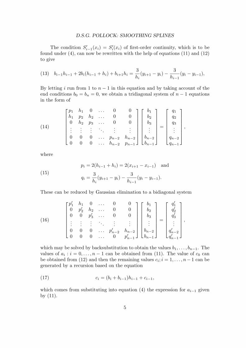
path of a certain stochastic differential equation of which the observations areaffected by noise. This is a startling result, and it provides a strong justificationfor the practice of representing trends with splines. The optimal degree ofsmoothing now becomes a function of the parameters of the underling stochasticdifferential equation and of the parameters of the noise process; and thereforethe element of judgment in fitting the curve is eliminated.
We shall begin this account by establishing the algorithm for an ordinaryinterpolating spline. Thereafter, we shall give a detailed exposition of theclassical smoothing spline of which the degree of smoothness is a matter ofchoice. In the final section, we shall give an account of a model-based methodof determining an optimal degree of smoothing.
It should be emphasised that a model-based procedure for determining thedegree of smoothing will prove superior to a judgmental procedure only if themodel has been appropriately specified. The specification of a model is itself amatter of judgment.
Cubic Spline Interpolation
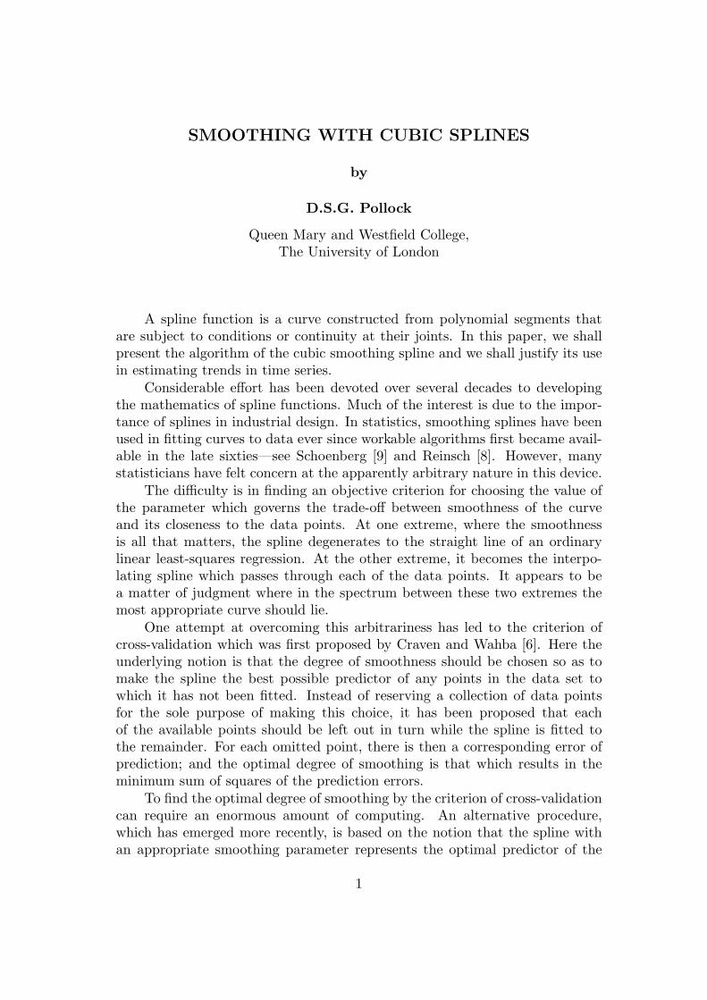
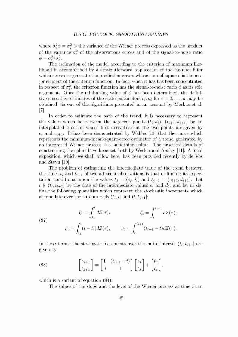
Imagine that we are given a set of co-ordinates (x0, y0), (x1, y1), . . . ,(xn, yn) of the function y = y(x) where the values of x are in ascending order.Our object is to bridge the gap between adjacent points (xi, yi), (xi+1, yi+1)using the cubic functions Si; i = 0, . . . , n−1 so as to piece together a curve withcontinuous first and second derivatives. Such a curve, which is described as acubic spline, is the mathematical equivalent of a draughtsman’s spline which isa thin strip of flexible wood used for drawing curves in engineering work. Thejunctions of the cubic segments, which correspond to the points at which thedraughtsman’s spline would be fixed, are known as knots or nodes.
x
y
Figure 1. A cubic spline.
2
D.S.G. POLLOCK: SMOOTHING SPLINES
We can express the function Si as
(1) Si(x) = ai(x− xi)3 + bi(x− xi)2 + ci(x− xi) + di,
where x ranges from xi to xi+1.The first and second derivatives of this function are
(2)S′i(x) = 3ai(x− xi)2 + 2bi(x− xi) + ci and
S′′i (x) = 6ai(x− xi) + 2bi.
The condition that the adjacent functions Si−1 and Si for i = 1, . . . , n shouldmeet at the point (xi, yi) is expressed in the equation
(3)Si−1(xi) = Si(xi) = yi or, equivalently,
ai−1h3i−1 + bi−1h
2i−1 + ci−1hi−1 + di−1 = di = yi,
where hi−1 = xi−xi−1. The condition that the first derivatives should be equalat the junction is expressed in the equation
(4)S′i−1(xi) = S′i(xi) or, equivalently,
3ai−1h2i−1 + 2bi−1hi−1 + ci−1 = ci;
and the condition that the second derivatives should be equal is expressed as
(5)S′′i−1(xi) = S′′i (xi) or, equivalently,
6ai−1hi−1 + 2bi−1 = 2bi.
We also need to specify the conditions which prevail at the end points(x0, y0) and (xn, yn). We can set the first derivatives of the cubic functions atthese points to the values of the corresponding derivatives of y = y(x) thus:
(6)S′0(x0) = c0
= y′(x0)and
S′n−1(xn) = cn
= y′(xn).
This is described as clamping the spline. By clamping the spline, we are intro-ducing additional information about the function y = y(x); and, therefore, wecan expect a better approximation. However, extra information of an equiva-lent nature can often be obtained by assessing the function at additional pointsclose to the ends.
If we leave the ends free, then the conditions
(7)S′′0 (x0) = 2b0
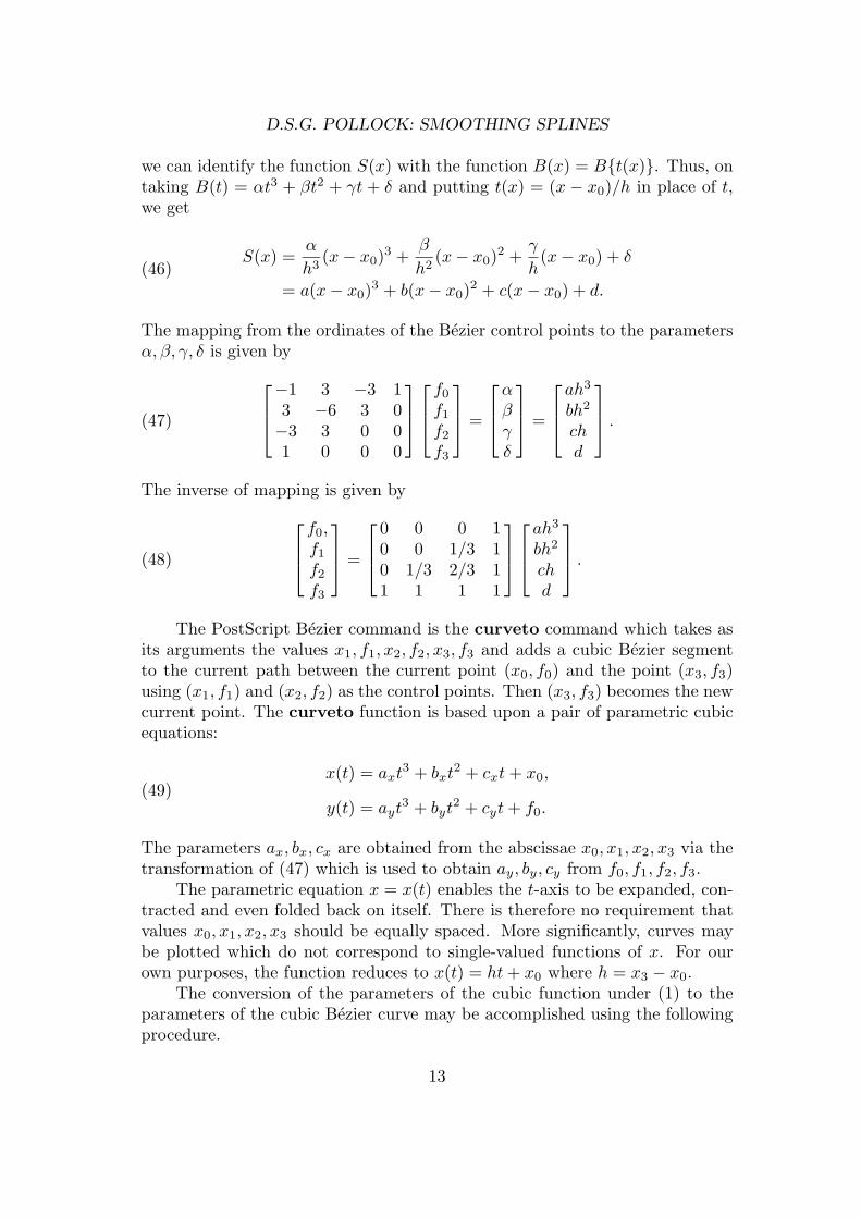
= 0and
S′′n−1(xn) = 2bn
= 0
3
D.S.G. POLLOCK: SMOOTHING SPLINES
will prevail. These imply that the spline is linear when it passes through theend points. We are likely to use the latter conditions when the informationabout the first derivatives of the function y = y(x) is hard to come by.
We shall begin by treating the case of the natural spline which has freeends. In this case, we know the values of b0 and bn, and we can begin bydetermining the remaining second-degree parameters b1, . . . , bn−1 from the datapoints y0, . . . , yn and from the conditions of continuity. Once we have foundthe values for the second-degree parameters, we can proceed to determine thevalues of the remaining parameters of the cubic segments.
Consider therefore the following four conditions relating to the ith segment:
(8)(i) Si(xi) = yi,
(iii) S′′i (xi) = 2bi,
(ii) Si(xi+1) = yi+1,
(iv) S′′i (xi+1) = 2bi+1.
If bi and bi+1 were known in advance, as they would be in the case of n =1, then these conditions would serve to specify uniquely the four parametersof Si. In the case of n > 1, the conditions of first-order continuity providethe necessary link between the segments which enables us to determine theparameters b1, . . . , bn−1 simultaneously.
The first of the four conditions specifies that
(9) di = yi.
The second condition specifies that aih3i + bih
2i + cihi + di = yi+1, whence we
get
(10) ci =yi+1 − yi
hi− aih2
i − bihi.
The third condition may be regarded as an identity. The fourth conditionspecifies that 6aihi + 2bi = 2bi+1, which gives
(11) ai =bi+1 − bi
3hi.
Putting this into (10) gives
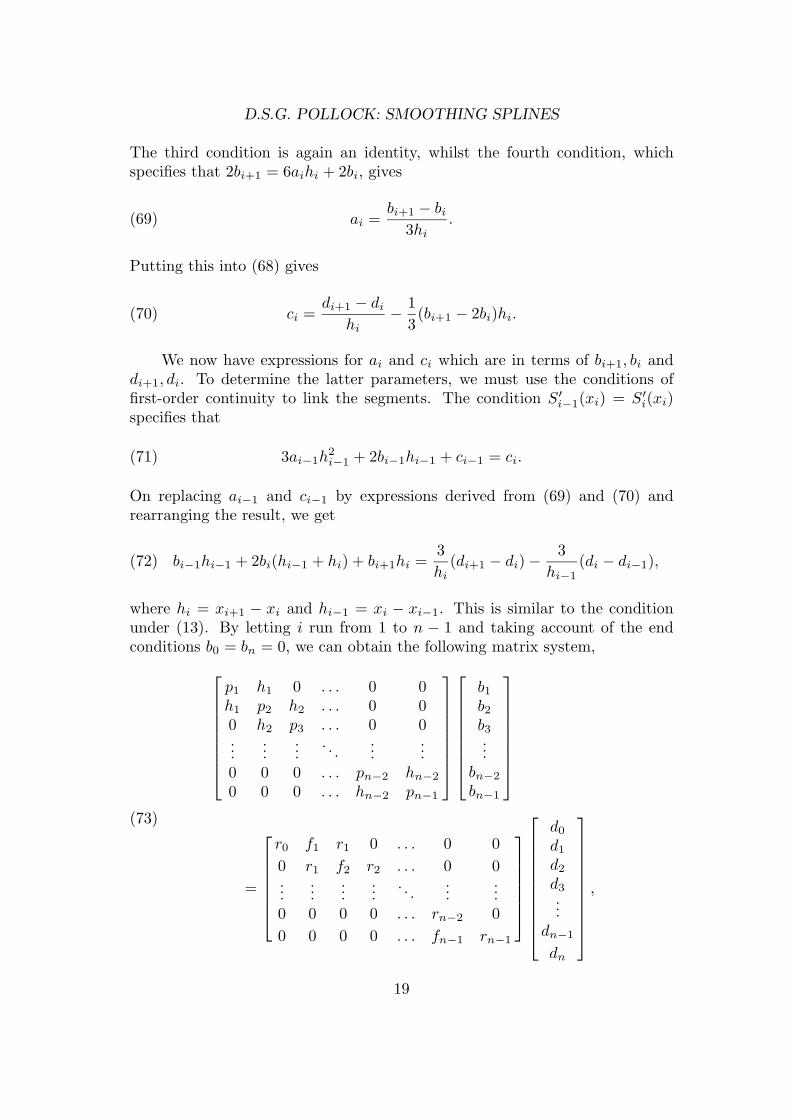
(12) ci =(yi+1 − yi)
hi− 1
3(bi+1 + 2bi)hi;
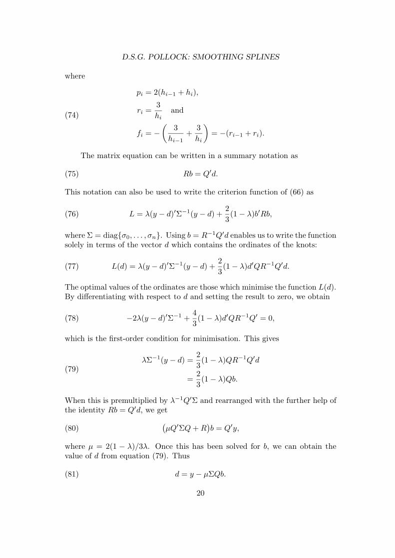
and thus we have succeeded in expressing the parameters of the ith segment interms of the second-order parameters bi+1, bi and the data values yi+1, yi.
4
D.S.G. POLLOCK: SMOOTHING SPLINES
The condition S′i−1(xi) = S′i(xi) of first-order continuity, which is to befound under (4), can now be rewritten with the help of equations (11) and (12)to give
(13) bi−1hi−1 + 2bi(hi−1 + hi) + bi+1hi =3
hi(yi+1 − yi)−
3
hi−1(yi − yi−1),
By letting i run from 1 to n− 1 in this equation and by taking account of theend conditions b0 = bn = 0, we obtain a tridiagonal system of n− 1 equationsin the form of
(14)
p1 h1 0 . . . 0 0h1 p2 h2 . . . 0 00 h2 p3 . . . 0 0...
......
. . ....
...0 0 0 . . . pn−2 hn−2
0 0 0 . . . hn−2 pn−1
b1b2b3...
bn−2
bn−1
=
q1
q2
q3...
qn−2
qn−1
,
where
(15)
pi = 2(hi−1 + hi) = 2(xi+1 − xi−1) and
qi =3
hi(yi+1 − yi)−
3
hi−1(yi − yi−1).
These can be reduced by Gaussian elimination to a bidiagonal system
(16)
p′1 h1 0 . . . 0 00 p′2 h2 . . . 0 00 0 p′3 . . . 0 0...
......
. . ....
...0 0 0 . . . p′n−2 hn−2
0 0 0 . . . 0 p′n−1
b1b2b3...
bn−2
bn−1
=
q′1q′2q′3...
q′n−2
q′n−1
,
which may be solved by backsubstitution to obtain the values b1, . . . , bn−1. Thevalues of ai : i = 0, . . . , n − 1 can be obtained from (11). The value of c0 canbe obtained from (12) and then the remaining values ci; i = 1, . . . , n− 1 can begenerated by a recursion based on the equation
(17) ci = (bi + bi−1)hi−1 + ci−1,
which comes from substituting into equation (4) the expression for ai−1 givenby (11).
5
D.S.G. POLLOCK: SMOOTHING SPLINES
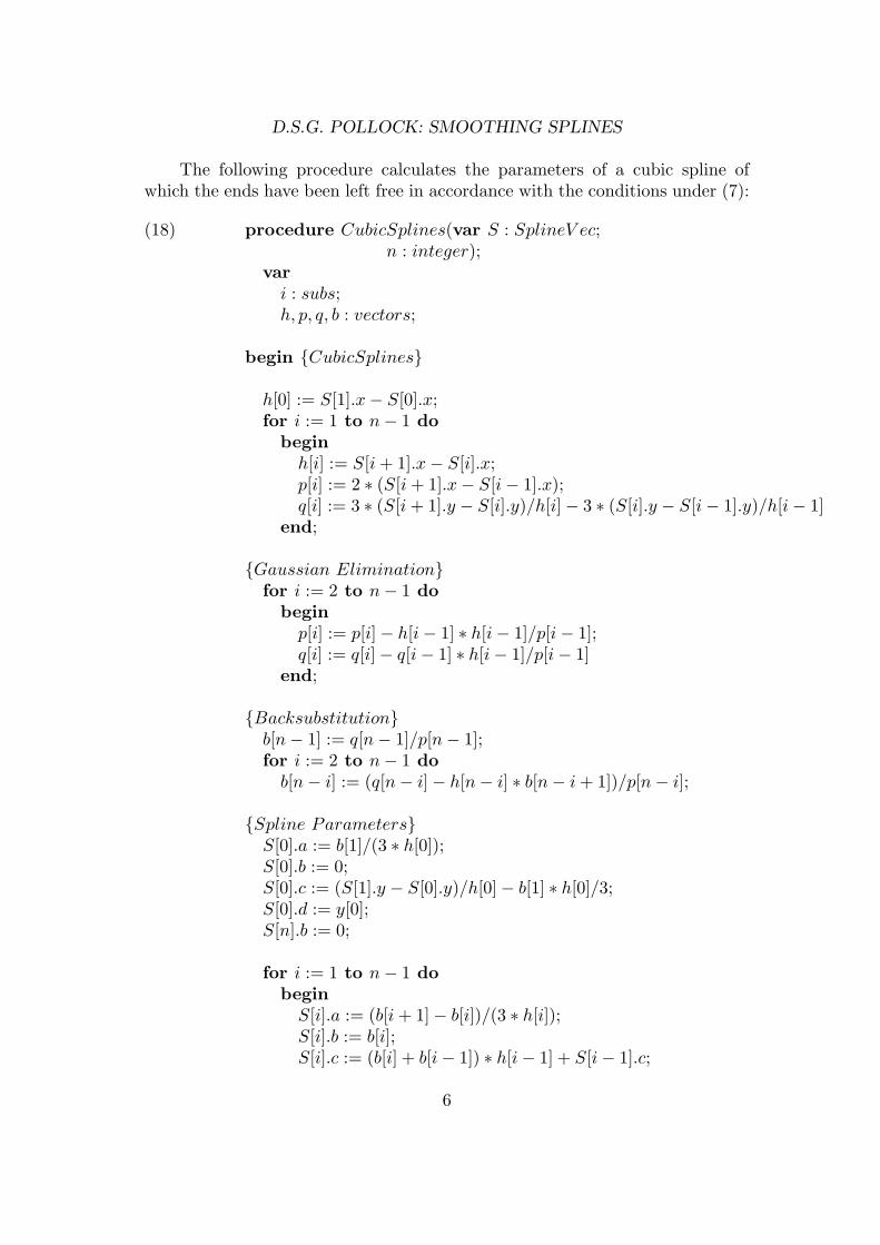
The following procedure calculates the parameters of a cubic spline ofwhich the ends have been left free in accordance with the conditions under (7):
(18) procedure CubicSplines(var S : SplineV ec;n : integer);
vari : subs;h, p, q, b : vectors;
begin {CubicSplines}
h[0] := S[1].x− S[0].x;for i := 1 to n− 1 do
beginh[i] := S[i+ 1].x− S[i].x;p[i] := 2 ∗ (S[i+ 1].x− S[i− 1].x);q[i] := 3 ∗ (S[i+ 1].y − S[i].y)/h[i]− 3 ∗ (S[i].y − S[i− 1].y)/h[i− 1]
end;
{Gaussian Elimination}for i := 2 to n− 1 do
beginp[i] := p[i]− h[i− 1] ∗ h[i− 1]/p[i− 1];q[i] := q[i]− q[i− 1] ∗ h[i− 1]/p[i− 1]
end;
{Backsubstitution}b[n− 1] := q[n− 1]/p[n− 1];for i := 2 to n− 1 dob[n− i] := (q[n− i]− h[n− i] ∗ b[n− i+ 1])/p[n− i];
{Spline Parameters}S[0].a := b[1]/(3 ∗ h[0]);S[0].b := 0;S[0].c := (S[1].y − S[0].y)/h[0]− b[1] ∗ h[0]/3;S[0].d := y[0];S[n].b := 0;
for i := 1 to n− 1 dobeginS[i].a := (b[i+ 1]− b[i])/(3 ∗ h[i]);S[i].b := b[i];S[i].c := (b[i] + b[i− 1]) ∗ h[i− 1] + S[i− 1].c;
6
D.S.G. POLLOCK: SMOOTHING SPLINES
S[i].d := y[i];end;
end; {CubicSplines}
The procedure must be placed in an environment containing the followingtype statements:
(19) typeSplineParameters = record
a, b, c, d, x, y : realend;
SplineV ec = array[0..dim] of SplineParameters;
At the beginning of the procedure, the record S[i] contains only the valuesof xi and yi which are held as S[i].x and S[i].y respectively. At the conclusionof the procedure, the parameters ai, bi, ci, di of the ith cubic segment are heldin S[i].a, S[i].b, S[i].c and S[i].d respectively.
Now let us consider the case where the ends of the spline are clamped.Then we know the values of c0 and cn, and we may begin by determining theremaining first-degree parameters c1, . . . , cn−1 from the data points y0, . . . , ynand from the continuity conditions. Consider therefore the following four con-ditions relating to the ith segment:
(20)(i) Si(xi) = yi,
(iii) S′i(xi) = ci,
(ii) Si(xi+1) = yi+1,
(iv) S′i(xi+1) = ci+1.
If ci and ci+1 were known in advance, as they would be in the case ofn = 1, then these four conditions would serve to specify the parameters of thesegment. The first and second conditions, which are the same as in the caseof the natural spline, lead to equation (10). The third condition is an identity,whilst the fourth condition specifies that
(21) ci+1 = 3aih2i + 2bihi + ci.
The equations (10) and (21) can be solved simultaneously to give
(22) ai =1
h2i
(ci + ci+1) +2
h3i
(yi − yi+1)
and
(23) bi =3
h2i
(yi+1 − yi)−1
hi(ci+1 + 2ci).
7
D.S.G. POLLOCK: SMOOTHING SPLINES
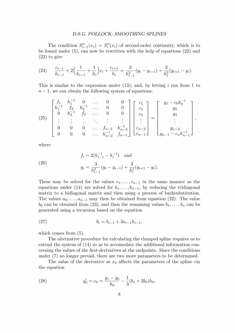
The condition S′′i−1(xi) = S′′i (xi) of second-order continuity, which is tobe found under (5), can now be rewritten with the help of equations (22) and(23) to give
(24)ci−1
hi−1+ 2( 1
hi−1+
1
hi
)ci +
ci+1
hi=
3
h2i−1
(yi − yi−1) +3
h2i
(yi+1 − yi).
This is similar to the expression under (13); and, by letting i run from 1 ton− 1, we can obtain the following system of equations:
(25)
f1 h−11 0 . . . 0 0
h−11 f2 h−1
2 . . . 0 00 h−1
2 f3 . . . 0 0...
......
. . ....
...0 0 0 . . . fn−2 h−1
n−2
0 0 0 . . . h−1n−2 fn−1
c1c2c3...
cn−2
cn−1
=
g1 − c0h−10
g2
g3...
gn−2
gn−1 − cnh−1n−1
,
where
(26)
fi = 2(h−1i−1 − h−1
i ) and
gi =3
h2i−1
(yi − yi−1) +3
h2i
(yi+1 − yi).
These may be solved for the values c1, . . . , cn−1 in the same manner as theequations under (14) are solved for b1, . . . , bn−1, by reducing the tridiagonalmatrix to a bidiagonal matrix and then using a process of backsubstitution.The values a0, . . . , an−1 may then be obtained from equation (22). The valueb0 can be obtained from (23), and then the remaining values b1, . . . , bn can begenerated using a recursion based on the equation
(27) bi = bi−1 + 3ai−1hi−1,
which comes from (5).The alternative procedure for calculating the clamped spline requires us to
extend the system of (14) so as to accomodate the additional information con-cerning the values of the first-derivatives at the endpoints. Since the conditionsunder (7) no longer prevail, there are two more parameters to be determined.
The value of the derivative at x0 affects the parameters of the spline viathe equation
(28) y′0 = c0 =y1 − y0
h0− 1
3(b1 + 2b0)h0,
8
D.S.G. POLLOCK: SMOOTHING SPLINES
which comes from combining the first condition under (6) with the equationunder (12). This becomes
(29) p0b0 + h0b1 = q0
when we define
(30) p0 = 2h0 and q0 =3
h0(y1 − y0)− 3y′0.
The value of the derivative at xn affects the parameters of the spline viathe equation
(31) y′n = cn = 3an−1h2n−1 + 2bn−1hn−1 + cn−1,
which comes from combining the second contition under (6) with the conditionunder (4). Using (11) and (12), we can rewrite this as
(32) y′n −(yn − yn−1)
hn−1=
2
3bnhn−1 +
1
3bn−1hn−1
which becomes
(33) hn−1bn−1 + pnbn = qn
when we define
(34) pn = 2hn and qn = 3y′n −3
hn−1(yn − yn−1).
The extended system can now be written as
(35)
p0 h0 0 . . . 0 0h0 p1 h1 . . . 0 00 h1 p2 . . . 0 0...
......
. . ....
...0 0 0 . . . pn−1 hn−1
0 0 0 . . . hn−1 pn
b0b1b2...
bn−1
bn
=
q0
q1
q2...
qn−1
qn
.
Cubic Splines and Bezier Curves
Parametric cubic splines have been much used in the past in ship-buildingand aircraft design and they have been used, to a lesser extent, in the design ofcar bodies. However, their suitability to an iterative design process is limited
9
D.S.G. POLLOCK: SMOOTHING SPLINES
by the fact that, if the location of one of the knots is altered, then the wholespline must be recalculated. In recent years, cubic splines have been replacedincreasingly in computer-aided design applications by the so-called cubic Beziercurve.
A testimony to the versatility of cubic Bezier curves is the fact that thePostScript [2] page-description language, which has been used in constructingthe letter forms on these pages, employs Bezier curve segments exclusively inconstructing curved paths, including very close approximations to circles.
The usual parametrisation of a Bezier curve differs from the parametri-sation of the cubic polynomial to be found under (1). Therefore, in order tomake use of the Bezier function provided by a PostScript-compatible printer,we need to establish the correspondence between the two sets of parameters.The Bezier function greatly facilitates the plotting of functions which can berepresented exactly or approximately by cubic segments.
The curve-drawing method of Bezier [4], [5] is based on a classical methodof approximation known as the Bernstein polynomial approximation. Let f(t)with t ∈ [0, 1] be an arbitrary real-valued function taking the values fk = f(tk)at the points tk = k/n; k = 0, . . . , n which are equally spaced in the interval[0, 1]. Then the Bernstein polynomial of degree n is defined by
(36) Bn(t) =n∑k=0
fkn!
k!(n− k)!tk(1− t)n−k.
The coefficients in this sum are just the terms of the expansion of the binomial
(37){t+ (1− t)
}n=
n∑k=0
n!
k!(n− k)!tk(1− t)n−k;
from which it can be seen that the sum of the coefficients is unity.Bernstein [3] used this polynomial in a classic proof of the Weierstrass
approximation theorem [12] which asserts that, for any ε > 0, there existsa polynomial Pn(t) of degree n = n(ε) such that |f(t) − Pn(t)| < ε. Theconsequence of Bernstein’s proof is that Bn(t) converges uniformly to f(t) in[0, 1] as n→∞.
The restriction of the functions to the interval [0, 1] is unessential to thetheorem. To see how it may be relieved, consider a continuous monotonictransformation x = x(t) defined over an interval bounded by x0 = x(0) andx1 = x(1). The inverse function t = t(x) exists; and, if f(x) = f{t(x)} andBn(x) = Bn{t(x)}, then Bn(x) converges uniformly to f(x) as Bn(t) convergesto f(t).
10
D.S.G. POLLOCK: SMOOTHING SPLINES
t
f
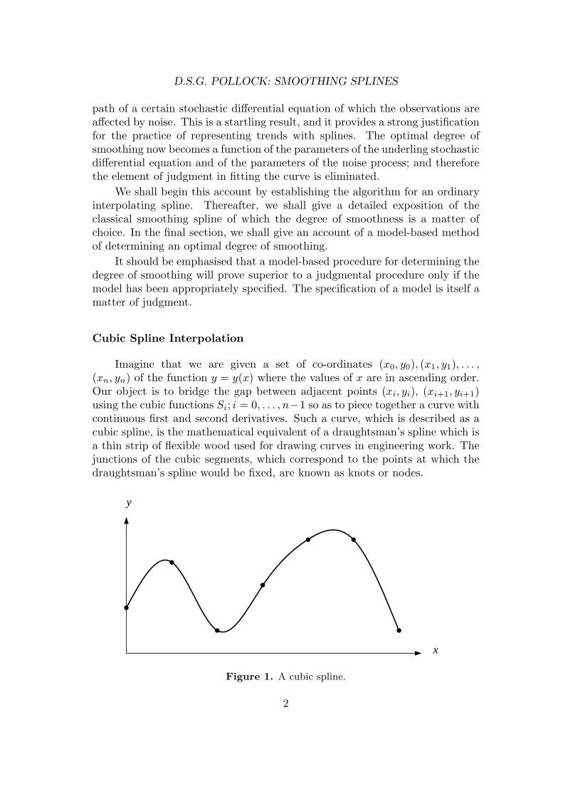
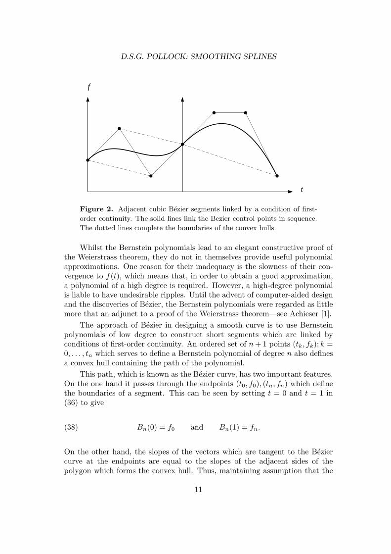
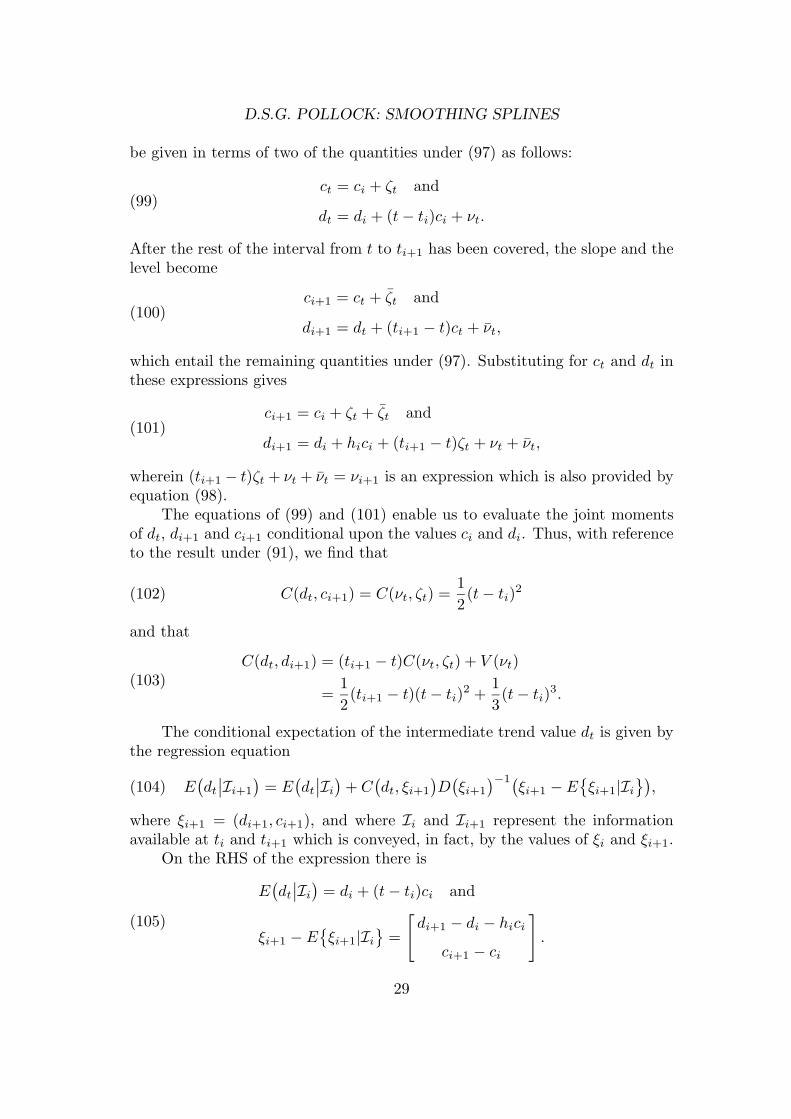
Figure 2. Adjacent cubic Bezier segments linked by a condition of first-
order continuity. The solid lines link the Bezier control points in sequence.
The dotted lines complete the boundaries of the convex hulls.
Whilst the Bernstein polynomials lead to an elegant constructive proof ofthe Weierstrass theorem, they do not in themselves provide useful polynomialapproximations. One reason for their inadequacy is the slowness of their con-vergence to f(t), which means that, in order to obtain a good approximation,a polynomial of a high degree is required. However, a high-degree polynomialis liable to have undesirable ripples. Until the advent of computer-aided designand the discoveries of Bezier, the Bernstein polynomials were regarded as littlemore that an adjunct to a proof of the Weierstrass theorem—see Achieser [1].
The approach of Bezier in designing a smooth curve is to use Bernsteinpolynomials of low degree to construct short segments which are linked byconditions of first-order continuity. An ordered set of n+ 1 points (tk, fk); k =0, . . . , tn which serves to define a Bernstein polynomial of degree n also definesa convex hull containing the path of the polynomial.
This path, which is known as the Bezier curve, has two important features.On the one hand it passes through the endpoints (t0, f0), (tn, fn) which definethe boundaries of a segment. This can be seen by setting t = 0 and t = 1 in(36) to give
(38) Bn(0) = f0 and Bn(1) = fn.
On the other hand, the slopes of the vectors which are tangent to the Beziercurve at the endpoints are equal to the slopes of the adjacent sides of thepolygon which forms the convex hull. Thus, maintaining assumption that the
11
D.S.G. POLLOCK: SMOOTHING SPLINES
n+ 1 points t0, . . . , tn are equally spaced in the interval [0, 1], we have
(39)
B′n(0) = n(f0 − f1)
=f0 − f1
t0 − t1and
B′n(1) = n(fn − fn−1)
=fn − fn−1
tn − tn−1.
If the endpoints of the Bezier curve are regarded as fixed, then the interme-diate points (t1, f1), . . . , (tn−1, fn−1) may be adjusted in an interactive mannerto make the Bezier curve conform to whatever shape is desired.
Example. Consider the cubic Bernstein polynomial
(40)B3(t) = f0(1− t)3 + 3f1t(1− t)2 + 3f2t
2(1− t) + f3t3
= αt3 + βt2 + γt+ δ.
Equating the coefficients of the powers of t shows that
(41)
α = f3 − 3f2 + 3f1 − f0,
β = 3f2 − 6f1 + 3f0,
γ = 3f1 + 3f0,
δ = f0.
Differentiating B3(t) with respect to t gives
(42) B′3(t) = −3f0(1− t)2 + 3f1t(1− 4t+ 3t2) + 3f2(2t− 3t2) + 3f3t2,
from which
(43) B′3(0) = 3(f0 − f1) and B′3(1) = 3(f3 − f2).
In order to exploit the Bezier command which is available in the PostScriptlanguage, we need to define the relationship between ordinates f0, f1, f2, f3 ofthe four control points of a cubic Bezier curve and the four parameters a, b, c, dof the representation of a cubic polynomial which is to be found under (1).
Let us imagine that the Bezier function B3(t) ranges from f0 to f3 as tranges from 0 to 1, and let
(44) S(x) = a(x− x0)3 + b(x− x0)2 + c(x− x0) + d
be a segment of the cubic spline which spans the gap between two points which,for ease of notation, we will denote by (x0, y0) and (x3, y3). Then, if we define
(45)x(t) = (x3 − x0)t+ x0
= ht+ x0,
12
D.S.G. POLLOCK: SMOOTHING SPLINES
we can identify the function S(x) with the function B(x) = B{t(x)}. Thus, ontaking B(t) = αt3 + βt2 + γt + δ and putting t(x) = (x − x0)/h in place of t,we get
(46)S(x) =
α
h3(x− x0)3 +
β
h2(x− x0)2 +
γ
h(x− x0) + δ
= a(x− x0)3 + b(x− x0)2 + c(x− x0) + d.
The mapping from the ordinates of the Bezier control points to the parametersα, β, γ, δ is given by
(47)
−1 3 −3 13 −6 3 0−3 3 0 01 0 0 0
f0
f1
f2
f3
=
αβγδ
=
ah3
bh2
chd
.The inverse of mapping is given by
(48)
f0,f1
f2
f3
=
0 0 0 10 0 1/3 10 1/3 2/3 11 1 1 1
ah3
bh2
chd
.The PostScript Bezier command is the curveto command which takes as
its arguments the values x1, f1, x2, f2, x3, f3 and adds a cubic Bezier segmentto the current path between the current point (x0, f0) and the point (x3, f3)using (x1, f1) and (x2, f2) as the control points. Then (x3, f3) becomes the newcurrent point. The curveto function is based upon a pair of parametric cubicequations:
(49)x(t) = axt
3 + bxt2 + cxt+ x0,
y(t) = ayt3 + byt
2 + cyt+ f0.
The parameters ax, bx, cx are obtained from the abscissae x0, x1, x2, x3 via thetransformation of (47) which is used to obtain ay, by, cy from f0, f1, f2, f3.
The parametric equation x = x(t) enables the t-axis to be expanded, con-tracted and even folded back on itself. There is therefore no requirement thatvalues x0, x1, x2, x3 should be equally spaced. More significantly, curves maybe plotted which do not correspond to single-valued functions of x. For ourown purposes, the function reduces to x(t) = ht+ x0 where h = x3 − x0.
The conversion of the parameters of the cubic function under (1) to theparameters of the cubic Bezier curve may be accomplished using the followingprocedure.
13
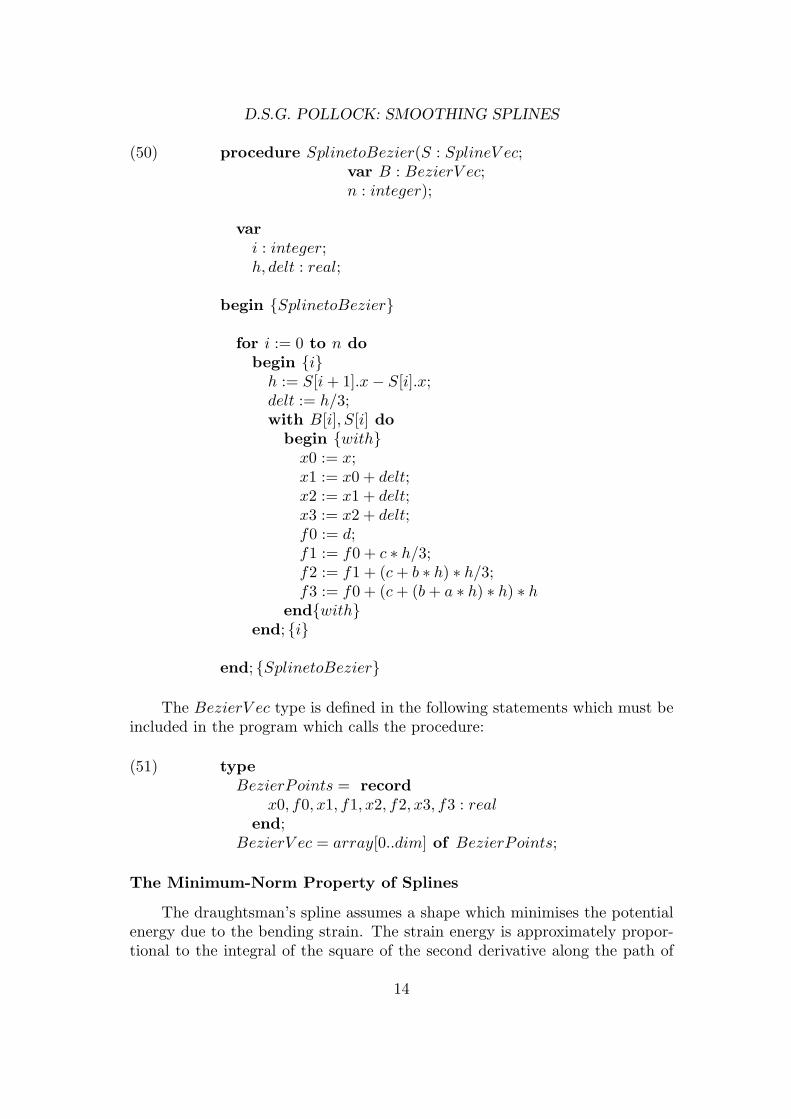
D.S.G. POLLOCK: SMOOTHING SPLINES
(50) procedure SplinetoBezier(S : SplineV ec;var B : BezierV ec;n : integer);
vari : integer;h, delt : real;
begin {SplinetoBezier}
for i := 0 to n dobegin {i}h := S[i+ 1].x− S[i].x;delt := h/3;with B[i], S[i] do
begin {with}x0 := x;x1 := x0 + delt;x2 := x1 + delt;x3 := x2 + delt;f0 := d;f1 := f0 + c ∗ h/3;f2 := f1 + (c+ b ∗ h) ∗ h/3;f3 := f0 + (c+ (b+ a ∗ h) ∗ h) ∗ h
end{with}end; {i}
end; {SplinetoBezier}
The BezierV ec type is defined in the following statements which must beincluded in the program which calls the procedure:
(51) typeBezierPoints = record
x0, f0, x1, f1, x2, f2, x3, f3 : realend;
BezierV ec = array[0..dim] of BezierPoints;
The Minimum-Norm Property of Splines
The draughtsman’s spline assumes a shape which minimises the potentialenergy due to the bending strain. The strain energy is approximately propor-tional to the integral of the square of the second derivative along the path of
14
D.S.G. POLLOCK: SMOOTHING SPLINES
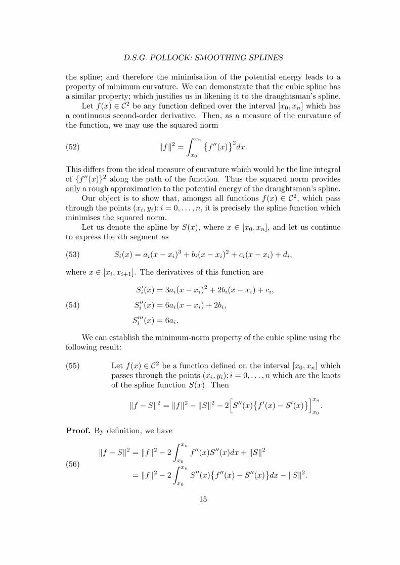
the spline; and therefore the minimisation of the potential energy leads to aproperty of minimum curvature. We can demonstrate that the cubic spline hasa similar property; which justifies us in likening it to the draughtsman’s spline.
Let f(x) ∈ C2 be any function defined over the interval [x0, xn] which hasa continuous second-order derivative. Then, as a measure of the curvature ofthe function, we may use the squared norm
(52) ‖f‖2 =
∫ xn
x0
{f ′′(x)
}2dx.
This differs from the ideal measure of curvature which would be the line integralof {f ′′(x)}2 along the path of the function. Thus the squared norm providesonly a rough approximation to the potential energy of the draughtsman’s spline.
Our object is to show that, amongst all functions f(x) ∈ C2, which passthrough the points (xi, yi); i = 0, . . . , n, it is precisely the spline function whichminimises the squared norm.
Let us denote the spline by S(x), where x ∈ [x0, xn], and let us continueto express the ith segment as
(53) Si(x) = ai(x− xi)3 + bi(x− xi)2 + ci(x− xi) + di,
where x ∈ [xi, xi+1]. The derivatives of this function are
(54)
S′i(x) = 3ai(x− xi)2 + 2bi(x− xi) + ci,
S′′i (x) = 6ai(x− xi) + 2bi,
S′′′i (x) = 6ai.
We can establish the minimum-norm property of the cubic spline using thefollowing result:
(55) Let f(x) ∈ C2 be a function defined on the interval [x0, xn] whichpasses through the points (xi, yi); i = 0, . . . , n which are the knotsof the spline function S(x). Then
‖f − S‖2 = ‖f‖2 − ‖S‖2 − 2[S′′(x)
{f ′(x)− S′(x)
}]xnx0
.
Proof. By definition, we have
(56)
‖f − S‖2 = ‖f‖2 − 2
∫ xn
x0
f ′′(x)S′′(x)dx+ ‖S‖2
= ‖f‖2 − 2
∫ xn
x0
S′′(x){f ′′(x)− S′′(x)
}dx− ‖S‖2.
15
D.S.G. POLLOCK: SMOOTHING SPLINES
Within this expression, we find, through integrating by parts, that
(57)
∫ xn
x0
S′′(x){f ′′(x)− S′′(x)
}dx =
[S′′(x)
{f ′(x)− S′(x)
}]xnx0
−∫ xn
x0
S′′′(x){f ′(x)− S′(x)
}dx.
Since S(x) consists of the cubic segments Si(x); i = 0, . . . , n− 1, it follows thatthe third derivative S′′′(x) is constant in each open interval (xi, xi+1) with avalue of S′′′i (x) = 6ai. Therefore
(58)
∫ xn
x0
S′′′(x){f ′(x)− S′(x)
}dx =
n−1∑i=0
∫ xi+1
xi
6ai{f ′(x)− S′(x)
}dx
=n−1∑i=0
6ai
[f(x)− S(x)
]xi+1
xi= 0,
since f(x) = S(x) at xi and xi+1; and hence (57) becomes
(59)
∫ xn
x0
S′′(x){f ′′(x)− S′′(x)
}dx =
[S′′(x)
{f ′(x)− S′(x)
}]xnx0
.
Putting this into (56) gives the result which we wish to prove.
Now consider the case of the natural spline which satisfies the conditionsS′′(x0) = 0 and S′′(xn) = 0. Putting these into the equality of (55) reduces itto
(60) ‖f − S‖2 = ‖f‖2 − ‖S‖2,
which demonstrates that ‖f‖2 ≥ ‖S‖2. In the case of a clamped spline withS′(x0) = f ′(x0) and S′(xn) = f ′(xn), the equality of (55) is also reduced tothat of (60). Thus we see that, in either case, the cubic spline has the minimum-norm property.
Smoothing Splines
The interpolating spline provides a useful way of approximating a smoothfunction f(x) ∈ C2 only when the data points lie along the path of the functionor very close to it. If the data is scattered at random in the vicinity of the path,then an interpolating polynomial, which is bound to follow the same randomfluctuations, will belie the nature of the underlying function. Therefore, in theinterests of smoothness, we may wish to allow the spline to depart from thedata points.
16

D.S.G. POLLOCK: SMOOTHING SPLINES
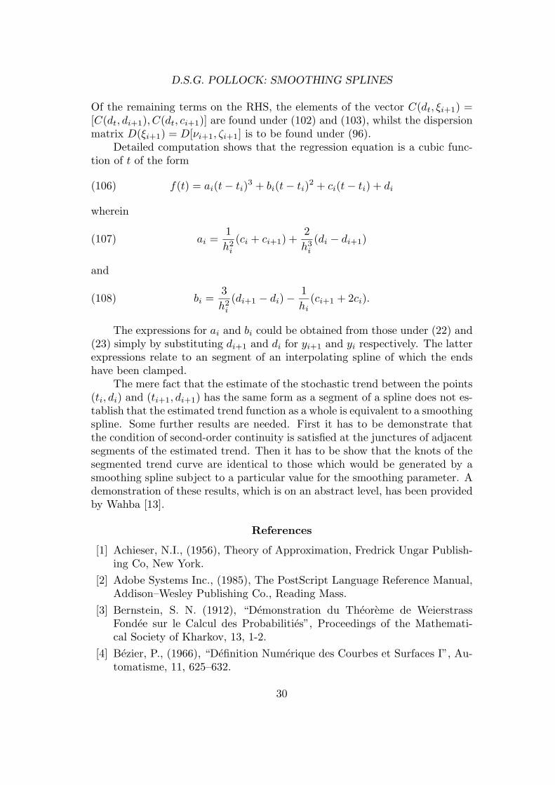
x
y
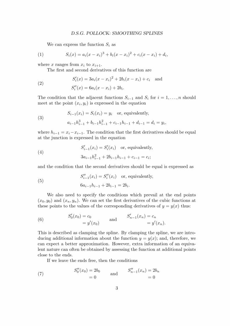
Figure 3. An cubic interpolating spline—the dotted path—and a cubic
smoothing spline—the continuous path. The smoothing parameter is λ =0.5.
We may imagine that the ordinates of the data are given by the equation
(61) yi = f(xi) + εi,
where εi; i = 0, . . . , n form a sequence of independently distributed randomvariables with V (εi) = σ2
i . In that case, we can attempt to reconstitute thefunction f(x) by constructing a spline function S(x) which minimises the valueof
(62) L = λn∑i=0
(yi − Siσi
)2
+ (1− λ)
∫ xn
x0
{S′′(x)
}2dx,
wherein Si = S(xi).The parameter λ ∈ [0, 1] reflects the relative importance which we give to
the conflicting objectives of remaining close to the data, on the one hand, andof obtaining a smooth curve, on the other hand. Notice that a linear functionsatisfies the equation
(63)
∫ xn
x0
{S′′(x)
}2dx = 0,
which suggests that, in the limiting case, where λ = 0 and where smoothnessis all that matters, the spline function S(x) will become a straight line. At theother extreme, where λ = 1 and where the closeness of the spline to the datais the only concern, we will obtain an interpolating spline which passes exactlythrough the data points.
17
D.S.G. POLLOCK: SMOOTHING SPLINES
Given the piecewise nature of the spline, we can write the integral in thesecond term on the RHS of (62) as
(64)
∫ xn
x0
{S′′(x)
}2dx =
n−1∑i=0
∫ xi+1
xi
{S′′i (x)
}2dx.
Since the spline is composed of cubic segments, the second derivative in anyinterval [xi, xi+1] is a linear function which changes from 2bi at xi to 2bi+1 atxi+1. Therefore we have
(65)
∫ xi+1
xi
{S′′i (x)
}2dx = 4
∫ hi
0
{bi
(1− x
hi
)+ bi+1
x
hi
}2
dx
=4hi3
(b2i + bibi+1 + b2i+1
),
where hi = xi+1 − xi; and the criterion function can be rewritten as
(66) L = λn∑i=0
(yi − diσi
)2
+ (1− λ)
n−1∑i=0
4hi3
(b2i + bibi+1 + b2i+1
),
wherein di = Si(xi).We shall treat the case of the natural spline which passes through the knots
(xi, di); i = 0, . . . , n and which satisfies the end conditions S′′(x0) = 2b0 = 0and S′′(xn) = 2bn = 0. The additional feature of the problem of fitting asmoothing spline, compared with that of fitting an interpolating spline, is theneed to determine the ordinates di; i = 0, . . . , n which are no longer providedby the data values yi; i = 0, . . . , n.
We can concentrate upon the problem of determining the parametersbi, di; i = 0, . . . , n if we eliminate the remaining parameters ai, ci; i = 1, . . . , n−1. Consider therefore the ith cubic segment which spans the gap between theknots (xi, di) and (xi+1, di+1) and which is subject to the following conditions:
(67)(i) Si(xi) = di,
(iii) S′′i (xi) = 2bi,
(ii) Si(xi+1) = di+1,
(iv) S′′i (xi+1) = 2bi+1.
The first condition may be regarded as an identity. The second condition,which specifies that aih
3i + bih
2i + cihi + di = di+1, gives us
(68) ci =di+1 − di
hi− aih2
i + bihi.
18
D.S.G. POLLOCK: SMOOTHING SPLINES
The third condition is again an identity, whilst the fourth condition, whichspecifies that 2bi+1 = 6aihi + 2bi, gives
(69) ai =bi+1 − bi
3hi.
Putting this into (68) gives
(70) ci =di+1 − di
hi− 1
3(bi+1 − 2bi)hi.
We now have expressions for ai and ci which are in terms of bi+1, bi anddi+1, di. To determine the latter parameters, we must use the conditions offirst-order continuity to link the segments. The condition S′i−1(xi) = S′i(xi)specifies that
(71) 3ai−1h2i−1 + 2bi−1hi−1 + ci−1 = ci.
On replacing ai−1 and ci−1 by expressions derived from (69) and (70) andrearranging the result, we get
(72) bi−1hi−1 + 2bi(hi−1 + hi) + bi+1hi =3
hi(di+1 − di)−
3
hi−1(di − di−1),
where hi = xi+1 − xi and hi−1 = xi − xi−1. This is similar to the conditionunder (13). By letting i run from 1 to n − 1 and taking account of the endconditions b0 = bn = 0, we can obtain the following matrix system,
(73)
p1 h1 0 . . . 0 0h1 p2 h2 . . . 0 00 h2 p3 . . . 0 0...
......
. . ....
...0 0 0 . . . pn−2 hn−2
0 0 0 . . . hn−2 pn−1
b1b2b3...
bn−2
bn−1
=
r0 f1 r1 0 . . . 0 0
0 r1 f2 r2 . . . 0 0...
......
.... . .
......
0 0 0 0 . . . rn−2 0
0 0 0 0 . . . fn−1 rn−1
d0
d1
d2
d3...
dn−1
dn
,
19
D.S.G. POLLOCK: SMOOTHING SPLINES
where
(74)
pi = 2(hi−1 + hi),
ri =3
hiand
fi = −(
3
hi−1+
3
hi
)= −(ri−1 + ri).
The matrix equation can be written in a summary notation as
(75) Rb = Q′d.
This notation can also be used to write the criterion function of (66) as
(76) L = λ(y − d)′Σ−1(y − d) +2
3(1− λ)b′Rb,
where Σ = diag{σ0, . . . , σn}. Using b = R−1Q′d enables us to write the functionsolely in terms of the vector d which contains the ordinates of the knots:
(77) L(d) = λ(y − d)′Σ−1(y − d) +2
3(1− λ)d′QR−1Q′d.
The optimal values of the ordinates are those which minimise the function L(d).By differentiating with respect to d and setting the result to zero, we obtain
(78) −2λ(y − d)′Σ−1 +4
3(1− λ)d′QR−1Q′ = 0,
which is the first-order condition for minimisation. This gives
(79)λΣ−1(y − d) =
2
3(1− λ)QR−1Q′d
=2
3(1− λ)Qb.
When this is premultiplied by λ−1Q′Σ and rearranged with the further help ofthe identity Rb = Q′d, we get
(80)(µQ′ΣQ+R
)b = Q′y,
where µ = 2(1 − λ)/3λ. Once this has been solved for b, we can obtain thevalue of d from equation (79). Thus
(81) d = y − µΣQb.
20
D.S.G. POLLOCK: SMOOTHING SPLINES
The value of the criterion function is given by
(82) L = (y − d)′Σ−1(y − d) = µ2b′Q′ΣQb.
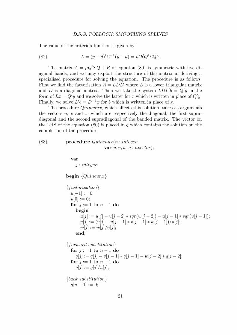
The matrix A = µQ′ΣQ + R of equation (80) is symmetric with five di-agonal bands; and we may exploit the structure of the matrix in deriving aspecialised procedure for solving the equation. The procedure is as follows.First we find the factorisation A = LDL′ where L is a lower triangular matrixand D is a diagonal matrix. Then we take the system LDL′b = Q′y in theform of Lx = Q′y and we solve the latter for x which is written in place of Q′y.Finally, we solve L′b = D−1x for b which is written in place of x.
The procedure Quincunx, which affects this solution, takes as argumentsthe vectors u, v and w which are respectively the diagonal, the first supra-diagonal and the second supradiagonal of the banded matrix. The vector onthe LHS of the equation (80) is placed in q which contains the solution on thecompletion of the procedure.
(83) procedure Quincunx(n : integer;var u, v, w, q : nvector);
varj : integer;
begin {Quincunx}
{factorisation}u[−1] := 0;u[0] := 0;for j := 1 to n− 1 do
beginu[j] := u[j]− u[j − 2] ∗ sqr(w[j − 2])− u[j − 1] ∗ sqr(v[j − 1]);v[j] := (v[j]− u[j − 1] ∗ v[j − 1] ∗ w[j − 1])/u[j];w[j] := w[j]/u[j];
end;
{forward substitution}for j := 1 to n− 1 doq[j] := q[j]− v[j − 1] ∗ q[j − 1]− w[j − 2] ∗ q[j − 2];
for j := 1 to n− 1 doq[j] := q[j]/u[j];
{back substitution}q[n+ 1] := 0;
21
D.S.G. POLLOCK: SMOOTHING SPLINES
q[n] := 0;for j := n− 1 downto 1 doq[j] := q[j]− v[j] ∗ q[j + 1]− w[j] ∗ q[j + 2];
end; {Quincunx}
The procedure which calculates the smoothing spline may be envisaged as ageneralisation of the procedure CubicSplines which calculates an interpolatingspline. In fact, by setting λ = 1, we obtain the interpolating spline.
The SmoothingSpline procedure is wasteful of computer memory, sincethere is no need to store the contents of the vectors r and f which have beenincluded in the code only for reasons of clarity. At any stage of the iteration ofthe index j, only two consecutive elements from each of these vectors are calledfor; and one of these elements may be calculated concurrently. However, thewaste of memory is of little concern unless one envisages applying the procedureto a very long run of data. In that case, it should be straightforward to modifythe procedure.
(84) procedure SmoothingSpline(var S : SplineV ec;sigma : vectors;lambda : real;n : integer);
varh, r, f, p, q, u, v, w : vectors;i, j : integer;mu : real;
begin {SmoothingSpline}mu := 2 ∗ (1− lambda)/(3 ∗ lambda);
h[0] := S[1].x− S[0].x;r[0] := 3/h[0];for i := 1 to n− 1 do
beginh[i] := S[i+ 1].x− S[i].x;r[i] := 3/h[i];f [i] := −(r[i− 1] + r[i]);p[i] := 2 ∗ (S[i+ 1].x− S[i− 1].x);q[i] := 3 ∗ (S[i+ 1].y − S[i].y)/h[i]− 3 ∗ (S[i].y − S[i− 1].y)/h[i− 1];
end;
for i := 1 to n− 1 do
22
D.S.G. POLLOCK: SMOOTHING SPLINES
beginu[i] := sqr(r[i− 1]) ∗ sigma[i− 1]
+sqr(f [i]) ∗ sigma[i] + sqr(r[i]) ∗ sigma[i+ 1];u[i] := mu ∗ u[i] + p[i];v[i] := f [i] ∗ r[i] ∗ sigma[i] + r[i] ∗ f [i+ 1] ∗ sigma[i+ 1];v[i] := mu ∗ v[i] + h[i];w[i] := mu ∗ r[i] ∗ r[i+ 1] ∗ sigma[i+ 1];
end;
Quincunx(n, u, v, w, q);
{Spline Parameters}S[0].d := S[0].y −mu ∗ r[0] ∗ q[1] ∗ sigma[0];S[1].d := S[1].y −mu ∗ (f [1] ∗ q[1] + r[1] ∗ q[2]) ∗ sigma[0];S[0].a := q[1]/(3 ∗ h[0]);S[0].b := 0;S[0].c := (S[1].d− S[0].d)/h[0]− q[1] ∗ h[0]/3;r[0] := 0;
for j := 1 to n− 1 dobeginS[j].a := (q[j + 1]− q[j])/(3 ∗ h[j]);S[j].b := q[j];S[j].c := (q[j] + q[j − 1]) ∗ h[j − 1] + S[j − 1].c;S[j].d := r[j − 1] ∗ q[j − 1] + f [j] ∗ q[j] + r[j] ∗ q[j + 1];S[j].d := y[j]−mu ∗ S[j].d ∗ sigma[j];
end;
end; {SmoothingSpline}
A Stochastic Model for the Smoothing Spline
The disadvantage of the smoothing spline is the extent to which the choiceof the value for the smoothing parameter remains a matter of judgment. Oneway of avoiding such judgments is to adopt an appropriate model of the processwhich has generated the data to which the spline is to be fitted. Then the valueof the smoothing parameter may be determined in the process of fitting themodel.
Since the smoothing spline is a continuous function, it is natural to imaginethat the process underlying the data is also continuous. A model which is likelyto prove appropriate to many circumstances is a so-called integrated Wienerprocess which is the continuous analogue of the familiar discrete-time unit-root autoregressive processes. To the continuous process, a discrete process is
25
D.S.G. POLLOCK: SMOOTHING SPLINES
added which represents a set of random errors of observation. Therefore, theestimation of the trend becomes a matter of signal extraction. A Wiener pro-cess Z(t) consists of an accumulation of independently distributed stochasticincrements. The path of Z(t) is continuous almost everywhere and differen-tiable almost nowhere. If dZ(t) stands for the increment of the process in theinfinitesimal interval dt, and if Z(a) is the value of the function at time a, thenthe value at time τ > a is given by
(85) Z(τ) = Z(a) +
∫ τ
a
dZ(t).
Moreover, it is assumed that the change in the value of the function over anyfinite interval (a, τ ] is a random variable with a zero expectation:
(86) E{Z(τ)− Z(a)
}= 0.
Let us write ds ∩ dt = ∅ whenever ds and dt represent non-overlappingintervals. Then the conditions affecting the increments may be expressed bywriting
(87) E{dZ(s)dZ(t)
}=
{0, if ds ∩ dt = ∅;σ2dt, if ds = dt.
These conditions imply that the variance of the change over the interval (a, τ ]is proportional to the length of the interval. Thus
(88)
V{Z(τ)− Z(a)
}=
∫ τ
s=a
∫ τ
t=a
E{dZ(s)dZ(t)
}=
∫ τ
t=a
σ2dt = σ2(τ − a).
The definite integrals of the Wiener process may be defined also in termsof the increments. The value of the first integral at time τ is given by
(89)
Z(1)(τ) = Z(1)(a) +
∫ τ
a
Z(t)dt
= Z(1)(a) + Z(a)(τ − a) +
∫ τ
a
(τ − t)dZ(t),
where the second equality comes via (85). The mth integral is
(90) Z(m)(τ) =m∑k=0
Z(k−m)(a)(τ − a)k
k!+
∫ τ
a
(τ − t)mm!
dZ(t).
26
D.S.G. POLLOCK: SMOOTHING SPLINES
The covariance of the changes Z(j)(τ) − Z(j)(a) and Z(k)(τ) − Z(k)(a) ofthe jth and the kth integrated processes derived from Z(t) is given by
(91)
C(a,τ)
{z(j), z(k)
}=
∫ τ
s=a
∫ τ
t=a
(τ − s)j(τ − t)kj!k!
E{dZ(s)dZ(t)
}= σ2
∫ τ
a
(τ − t)j(τ − t)kj!k!
dt = σ2 (τ − a)j+k+1
(j + k + 1)!j!k!.
The simplest stochastic model which can give rise to the smoothing splineis one in which the generic observation is depicted as the sum of a tend com-ponent described by an integrated Wiener process and a random error takenfrom a discrete white-noise sequence. We may imagine that the observationsy0, y1, . . . , yn are made at the times t0, t1, . . . , tn. The interval between ti+1
and ti is hi = ti+1 − ti which, for the sake of generality, is allowed to vary.These points in time replace the abscissae x0, x1, . . . , xn which have, hitherto,formed part of our observations.
In order to conform to our existing notation, we define
(92) ci = Z(ti) and di = Z(1)(ti)
to be, respectively, the slope of the trend component and its level at time ti,where Z(ti) and Z(1)(ti) are described by equations (85) and (89). Also wedefine
(93) ζi+1 =
∫ ti+1
ti
dZ(t) and νi+1 =
∫ ti+1
ti
(ti+1 − t)dZ(t).
Then the model of the underlying trend can be written is state-space form asfollows:
(94)
[di+1
ci+1
]=
[1 hi
0 1
] [di
ci
]+
[νi+1
ζi+1
],
whilst the equation of the corresponding observation is
(95) yi+1 = [ 1 0 ]
[di+1
ci+1
]+ εi+1.
Using the result under (92), we find that the dispersion matrix for the statedisturbances is
(96) D
[νi+1
ζi+1
]= σ2
εφ
[ 13h
3i
12h
2i
12h
2i hi
],
27
D.S.G. POLLOCK: SMOOTHING SPLINES
where σ2εφ = σ2
ζ is the variance of the Wiener process expressed as the product
of the variance σ2ε of the observations errors and of the signal-to-noise ratio
φ = σ2ζ/σ
2ε .
The estimation of the model according to the criterion of maximum like-lihood is accomplished by a straightforward application of the Kalman filterwhich serves to generate the prediction errors whose sum of squares is the ma-jor element of the criterion function. In fact, when it has has been concentratedin respect of σ2
ε , the criterion function has the signal-to-noise ratio φ as its soleargument. Once the minimising value of φ has been determined, the defini-tive smoothed estimates of the state parameters ci, di for i = 0, . . . , n may beobtained via one of the algorithms presented in an account by Merkus et al.[7].
In order to estimate the path of the trend, it is necessary to representthe values which lie between the adjacent points (ti, di), (ti+1, di+1) by aninterpolated function whose first derivatives at the two points are given byci and ci+1. It has been demonstrated by Wahba [13] that the curve whichrepresents the minimum-mean-square-error estimator of a trend generated byan integrated Wiener process is a smoothing spline. The practical details ofconstructing the spline have been set forth by Wecker and Ansley [11]. A lucidexposition, which we shall follow here, has been provided recently by de Vosand Steyn [10].
The problem of estimating the intermediate value of the trend betweenthe times ti and ti+1 of two adjacent observations is that of finding its expec-tation conditional upon the values ξi = (ci, di) and ξi+1 = (ci+1, di+1). Lett ∈ (ti, ti+1] be the date of the intermediate values ct and dt; and let us de-fine the following quantities which represent the stochastic increments whichaccumulate over the sub-intervals (ti, t] and (t, ti+1]:
(97)
ζt =
∫ t
t1
dZ(τ),
νt =
∫ t
t1
(t− ti)dZ(τ),
ζt =
∫ ti+1
t
dZ(τ),
νt =
∫ ti+1
t
(ti+1 − t)dZ(τ).
In these terms, the stochastic increments over the entire interval (ti, ti+1] aregiven by
(98)
[νi+1
ζi+1
]=
[1 (ti+1 − t)0 1
] [νt
ζt
]+
[νt
ζt
],
which is a variant of equation (94).
The values of the slope and the level of the Wiener process at time t can
28
D.S.G. POLLOCK: SMOOTHING SPLINES
be given in terms of two of the quantities under (97) as follows:
(99)ct = ci + ζt and
dt = di + (t− ti)ci + νt.
After the rest of the interval from t to ti+1 has been covered, the slope and thelevel become
(100)ci+1 = ct + ζt and
di+1 = dt + (ti+1 − t)ct + νt,
which entail the remaining quantities under (97). Substituting for ct and dt inthese expressions gives
(101)ci+1 = ci + ζt + ζt and
di+1 = di + hici + (ti+1 − t)ζt + νt + νt,
wherein (ti+1 − t)ζt + νt + νt = νi+1 is an expression which is also provided byequation (98).
The equations of (99) and (101) enable us to evaluate the joint momentsof dt, di+1 and ci+1 conditional upon the values ci and di. Thus, with referenceto the result under (91), we find that
(102) C(dt, ci+1) = C(νt, ζt) =1
2(t− ti)2
and that
(103)C(dt, di+1) = (ti+1 − t)C(νt, ζt) + V (νt)
=1
2(ti+1 − t)(t− ti)2 +
1
3(t− ti)3.
The conditional expectation of the intermediate trend value dt is given bythe regression equation
(104) E(dt∣∣Ii+1
)= E
(dt∣∣Ii)+ C
(dt, ξi+1
)D(ξi+1
)−1(ξi+1 − E
{ξi+1|Ii
}),
where ξi+1 = (di+1, ci+1), and where Ii and Ii+1 represent the informationavailable at ti and ti+1 which is conveyed, in fact, by the values of ξi and ξi+1.
On the RHS of the expression there is
(105)
E(dt∣∣Ii) = di + (t− ti)ci and
ξi+1 − E{ξi+1|Ii
}=
[di+1 − di − hici
ci+1 − ci
].
29
D.S.G. POLLOCK: SMOOTHING SPLINES
Of the remaining terms on the RHS, the elements of the vector C(dt, ξi+1) =[C(dt, di+1), C(dt, ci+1)] are found under (102) and (103), whilst the dispersionmatrix D(ξi+1) = D[νi+1, ζi+1] is to be found under (96).
Detailed computation shows that the regression equation is a cubic func-tion of t of the form
(106) f(t) = ai(t− ti)3 + bi(t− ti)2 + ci(t− ti) + di
wherein
(107) ai =1
h2i
(ci + ci+1) +2
h3i
(di − di+1)
and
(108) bi =3
h2i
(di+1 − di)−1
hi(ci+1 + 2ci).
The expressions for ai and bi could be obtained from those under (22) and(23) simply by substituting di+1 and di for yi+1 and yi respectively. The latterexpressions relate to an segment of an interpolating spline of which the endshave been clamped.
The mere fact that the estimate of the stochastic trend between the points(ti, di) and (ti+1, di+1) has the same form as a segment of a spline does not es-tablish that the estimated trend function as a whole is equivalent to a smoothingspline. Some further results are needed. First it has to be demonstrate thatthe condition of second-order continuity is satisfied at the junctures of adjacentsegments of the estimated trend. Then it has to be show that the knots of thesegmented trend curve are identical to those which would be generated by asmoothing spline subject to a particular value for the smoothing parameter. Ademonstration of these results, which is on an abstract level, has been providedby Wahba [13].
References
[1] Achieser, N.I., (1956), Theory of Approximation, Fredrick Ungar Publish-ing Co, New York.
[2] Adobe Systems Inc., (1985), The PostScript Language Reference Manual,Addison–Wesley Publishing Co., Reading Mass.
[3] Bernstein, S. N. (1912), “Demonstration du Theoreme de WeierstrassFondee sur le Calcul des Probabilities”, Proceedings of the Mathemati-cal Society of Kharkov, 13, 1-2.
[4] Bezier, P., (1966), “Definition Numerique des Courbes et Surfaces I”, Au-tomatisme, 11, 625–632.
30
D.S.G. POLLOCK: SMOOTHING SPLINES
[5] Bezier, P., (1967), “Definition Numerique des Courbes et Surfaces II”,Automatisme”, 12, 17–21.
[6] Craven, P. and Grace Wahba, (1979), “Smoothing Noisy Data with SplineFunctions: Estimating the Correct Degree of Smoothing by the Method ofGeneralised Cross-Validation”, Numerische Mathematik, 31, 377–403.
[7] Merkus, H.R., D.S.G. Pollock and A.F. de Vos, (1991) “A Synopsis ofthe Smoothing Formulae Associated with the Kalman Filter”, Discussionpaper No. 246 of the Department of Economics of Queen Mary College,forthcoming in Computer Science in Economics and Management.
[8] Reinsch, (1967),“Smoothing by Spline Functions”, Numerische Mathe-matik, 10, 177–183.
[9] Schoenberg, (1964), “Spline Functions and the Problem of Graduation”,Proc. Nat. Acad. Sci., 52, 947–950.
[10] De Vos, A.F. and I.J. Steyn, (1990), ”Stochastic Nonlinearity: A FirmBasis for the Flexible Functional Form”, Research Memorandum 1990-13,Vrije Universiteit Amsterdam.
[11] Wecker, W.P. and C.F. Ansley, (1983),“The Signal Extraction Approachto Nonlinear Regression and Spline Smoothing”,Journal of the AmericanStatistical Association, 78, 81–89.
[12] Weierstrass, K., (1885), “uber die analytische Darstellbarkheit sogenannterwillhulicher Functionen einer reellen Veranderlichen”, Berliner Berichte.
[13] Wahba, Grace, (1987), “Improper Priors, Spline Smoothing and the Prob-lem of Guarding against Model Errors in Regression”, Journal of the RoyalStatistical Society, Series B . 40, 364–372.
31
D.S.G. POLLOCK: SMOOTHING SPLINES
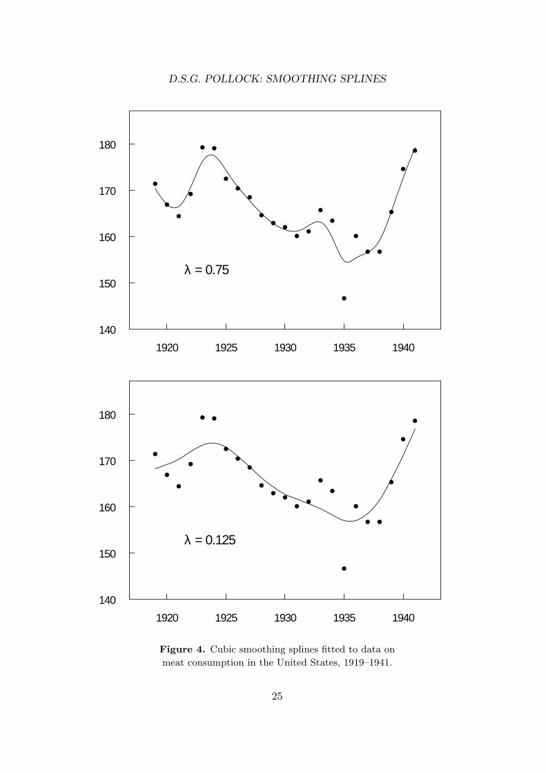
1920 1925 1930 1935 1940 140
150
160
170
180
λ = 0.75
1920 1925 1930 1935 1940 140
150
160
170
180
λ = 0.125
Figure 4. Cubic smoothing splines fitted to data on
meat consumption in the United States, 1919–1941.
25
D.S.G. POLLOCK: SMOOTHING SPLINES
SMOOTHING WITH CUBIC SPLINES
by
D.S.G. Pollock
Queen Mary and Westfield College,The University of London
This paper presents the algorithms of the cubic interpolating spline and the
smoothing spline together with their implementations in Pascal.
The smoothing spline can be used for estimating trends in time series.
The Pascal code makes use of the facility for constructing cubic Bezier
curves which is available in the PostScript graphics language.
The interpolating spline is controlled by a single parameter which gov-
erns the trade-off between the smoothness of the curve and its closeness to
the data points. Users must rely on their own judgment in choosing a value
for this parameter.
Some statisticians have voiced concern about placing such reliance
upon the user’s judgment; and various criteria have been proposed for de-
termining the degree of smoothness automatically. In the final section of
the paper, there is a brief account of the model-based approach to spline
smoothing which has emerged in recent years and which is still being de-
veloped.
Address for correspondence:
D.S.G. PollockDepartment of EconomicsQueen Mary CollegeUniversity of LondonMile End RoadLondon E1 4 NS
Tel : +44-71-975-5096Fax : +44-71-975-5500